Statistical Tools for Weld Defect Evaluation in Radiographic Testing

Nafaâ NACEREDDINE, Mourad TRIDI, LTSI, Centre de Recherche en Soudage et Contrôle, Chéraga, Alger, Algérie

Latifa HAMAMI, Dpt Electronique, Ecole Nationale Polytechnique, El-Harrach, Alger, Algérie

Djemel ZIOU, DMI, Faculté des sciences, Université de Sherbrooke, Sherbrooke, Québec, Canada

Abstract. A reliable detection of defects in welded joints is one of the most important tasks in non-destructive testing by radiography, since the human factor still has a decisive influence on the evaluation of defects on the film. An incorrect classification may disapprove a piece in good conditions or approve a piece with discontinuities exceeding the limit established by the applicable standards. The progresses in computer science and the artificial intelligence techniques have allowed the welded joint quality interpretation to be carried out by using pattern recognition tools, making the system of the weld inspection more reliable, reproducible and faster. In this work, we develop and implement algorithms based on statistical approaches for segmentation and classification of the weld defects. Because of the complex nature of the considered images and so that the extracted defect area represents the most accurately possible the real defect, and that the detected defect corresponds as well as possible to its real class, the choice of the algorithms must be very judicious. In order to achieve this, a comparative study of the various segmentation and classification methods was performed to demonstrate the advantages of the ones in comparison with the others giving to the most optimal combinations. Key words. Weld defect, segmentation, pattern recognition, statistical methods, performance criteria

1. Introduction

A reliable detection of defects in welded joints is one of the most important tasks in non-destructive testing by radiography, since the human factor still has a decisive influence on the evaluation of defects on the film. An incorrect classification may disapprove a piece in good conditions or approve a piece with discontinuities exceeding the limit established by the applicable standards [1].

The expert radiograph has as role to inspect each film in order to detect the presence of possible defects which he must then identify and measure. This work is made particularly delicate because of a low dimension of certain defects, a bad contrast and a noised nature of the radiographic film. The expert often works in extreme cases of the visual system and, that is why the subjectivity in the mechanisms of detection and measurement is not negligible.

Perfect knowledge of the geometry of these weld defects is an important step which is essential to appreciate the quality of the weld [2].

ECNDT 2006 - Mo.2.4.4

1

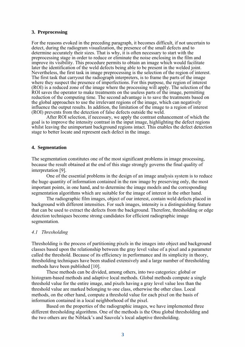
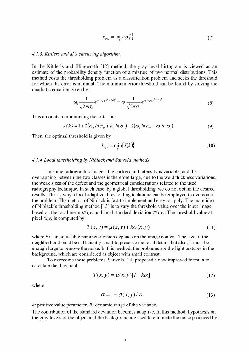
The progresses in computer science and the artificial intelligence techniques have allowed the defect classification to be carried out by using pattern recognition tools, which make the process automatic and more reliable, as it is not a subjective analysis [1]. Automatic defect detection is normally carried out by a well known pattern recognition technique, the steps of which are illustrated in Fig. 1: Image acquisition, pre-processing, segmentation, feature extraction, and classification [3]. After digitizing the radiographic image, the pre-processing is devoted to improving the quality of the image in order to better recognize defects (e.g., noise removal, integration, contrast enhancement, etc.). The segmentation process divides the digital image into disjoint regions with the purpose of separating the parts of interest from the rest of the scene. The present investigation uses the segmentation process based on global and local thresholding in one part [4] [5], and the edge detection by employing a method based on the maximization of the likelihood in the other part [6]. Subsequently, the feature extraction is centred principally around the measurement of invariant attributes deduced from moment and geometric parameters calculation of the regions of interest [7].

Finally, the classification assigns each segmented region according to the extracted features to pre-established category of weld defect. Typically, in defect detection in welded joints, four categories of defects can be distinguished, according to their shape. For this purpose, neural network paradigms and the Expectation Maximization (EM) algorithm [8] will be used and compared in terms of performance.

Fig. 1 The weld radiographic film formation and the automatic computer-aided system to defect detection and recognition

2. Digitization

Generally, the radiographic films are very dark and their density is rather large, therefore an ordinary scanner cannot give a sufficient lighting through a radiogram. Of course, specialized scanners adapted to take high quality copies of radiograms exist, but they are expensive. Here, we have used a scanner AGFA Arcus II, (800 dpi, 256 gray levels). The major part of the radiographic films that we have digitized, were extracted from the standard films provided by International Institute of Welding (IIW). After digitization, the principal characteristics of our images are: • Small contrast between the background and the weld defect regions. These last are

characterized by unsharpened and blurred edges. • Pronounced granularity due to digitization and the type of film used in industrial

radiographic testing. • Presence of background gradient of image characterizing the thickness variation of the

irradiated component part.

DIGITIZATION PREPROCESSING

SEGMENTATION FEATURE EXTRACTION

DEFECT CLASSIFICATION

X ray or gamma ray source

Rays

Weld joint

Weld defect

Film

IMAGE FORMATION

2

3. Preprocessing

For the reasons evoked in the preceding paragraph, it becomes difficult, if not uncertain to detect, during the radiogram visualization, the presence of the small defects and to determine accurately their sizes. That is why, it is often necessary to start with the preprocessing stage in order to reduce or eliminate the noise enclosing in the film and improve its visibility. This procedure permits to obtain an image which would facilitate later the identification of the weld defects being able to be present in the welded joint. Nevertheless, the first task in image preprocessing is the selection of the region of interest. The first task that carryout the radiograph interpreters, is to frame the parts of the image where they suspect the presence of imperfections. For this purpose, the region of interest (ROI) is a reduced zone of the image where the processing will apply. The selection of the ROI saves the operator to make treatments on the useless parts of the image, permitting reduction of the computing time. The second advantage is to save the treatments based on the global approaches to use the irrelevant regions of the image, which can negatively influence the output results. In addition, the limitation of the image to a region of interest (ROI) prevents from the detection of false defects outside the weld.

After ROI selection, if necessary, we apply the contrast enhancement of which the goal is to improve the intensity contrast in the input image, highlighting the defect regions whilst leaving the unimportant background regions intact. This enables the defect detection stage to better locate and represent each defect in the image.

4. Segmentation

The segmentation constitutes one of the most significant problems in image processing, because the result obtained at the end of this stage strongly governs the final quality of interpretation [9].

One of the essential problems in the design of an image analysis system is to reduce the huge quantity of information contained in the raw image by preserving only, the most important points, in one hand, and to determine the image models and the corresponding segmentation algorithms which are suitable for the image of interest in the other hand.

The radiographic film images, object of our interest, contain weld defects placed in background with different intensities. For such images, intensity is a distinguishing feature that can be used to extract the defects from the background. Therefore, thresholding or edge detection techniques become strong candidates for efficient radiographic image segmentation.

4.1 Thresholding

Thresholding is the process of partitioning pixels in the images into object and background classes based upon the relationship between the gray level value of a pixel and a parameter called the threshold. Because of its efficiency in performance and its simplicity in theory, thresholding techniques have been studied extensively and a large number of thresholding methods have been published [10].

These methods can be divided, among others, into two categories: global or histogram-based methods and adaptive local methods. Global methods compute a single threshold value for the entire image, and pixels having a gray level value less than the threshold value are marked belonging to one class, otherwise the other class. Local methods, on the other hand, compute a threshold value for each pixel on the basis of information contained in a local neighborhood of the pixel.

Based on the properties of the radiographic images, we have implemented three different thresholding algorithms. One of the methods is the Otsu global thresholding and the two others are the Niblack’s and Sauvola’s local adaptive thresholding.

3

4.1.1 Definitions

The gray level histogram is considered as probability distribution function

∑=

=≥=1

0

1 ,0 ,/L-

iiiii ppNhp (1)

where {0,1,2,…,L-1} denote the gray levels. The number of pixels in level i is denoted by hi and the total number of pixels is denoted by N.

Suppose we divide the pixels into two classes C0 and C1 by a threshold value at k. C0 denotes pixels with levels [0,1,…,k] and C1 denotes pixels with levels [k+1,…,L-1]. The probabilities of class occurrences ω, class mean levels μ and class variance for both classes are given by:

20

21

1

21

21

0

20

20

01

1

110

00

0

1

11

00

)( ; )(

;1

/ /

1

σσμσμσ

ωω

ω

−=−=−=

−−===

−===

∑∑

∑∑

∑∑

−

+==

−

+==

−

+==

T

L

kii

k

ii

kTL

kii

k

ii

L

kii

k

ii

pipi

ωμμip μ ;ipμ

; ωp ;pω

(2)

where

( )∑∑∑−

=

−

==

−===1

0

221

00

; ; L

iiTT

L

iiT

k

iik piipip μσμμ (3)

μT and σT are respectively the total mean and standard deviation.

4.1.2 Otsu’s variance method

Otsu [11] suggested minimizing the weighted sum of within-class variances of the object and background pixels to establish an optimum threshold. Recall that minimization of within-class variances is equivalent to maximization of between-class variance. Thus, a criterion measure is introduced by Otsu:

2T

2B σση /= (4)

where

( ) ( )211

200

2TTB μμωμμωσ −+−= (5)

is the between-class variance which can be simplified to

( )22110

2B μμωωσ −= (6)

The optimal threshold kopt is given by maximizing η or equivalently maximizing 2Bσ , since

2Tσ is independent of k.

4

{ }2Bkoptk σmax= (7)

4.1.3. Kittlers and al’s clustering algorithm

In the Kittler’s and Illingworth [12] method, the gray level histogram is viewed as an estimate of the probability density function of a mixture of two normal distributions. This method costs the thresholding problem as a classification problem and seeks the threshold for which the error is minimal. The minimum error threshold can be found by solving the quadratic equation given by:

21

21

20

20 2

11

2

00 2

121 σμσμ

σπω

σπω /)i(/)i( ee −−−− = (8)

This amounts to minimizing the criterion:

( ) ( )11001100 221 ωωωωσωσω lnln lnln)k(J +−++= (9)

Then, the optimal threshold is given by

( ){ }kJkkopt min= (10)

4.1.4 Local thresholding by Niblack and Sauvola methods

In some radiographic images, the background intensity is variable, and the overlapping between the two classes is therefore large, due to the weld thickness variations, the weak sizes of the defect and the geometrical considerations related to the used radiography technique. In such case, by a global thresholding, we do not obtain the desired results. That is why a local adaptive thresholding technique can be employed to overcome the problem. The method of Niblack is fast to implement and easy to apply. The main idea of Niblack’s thresholding method [13] is to vary the threshold value over the input image, based on the local mean μ(x,y) and local standard deviation σ(x,y). The threshold value at pixel (x,y) is computed by

),(),(),( yxkyxyxT σμ += (11)

where k is an adjustable parameter which depends on the image content. The size of the neighborhood must be sufficiently small to preserve the local details but also, it must be enough large to remove the noise. In this method, the problems are the light textures in the background, which are considered as object with small contrast.

To overcome these problems, Sauvola [14] proposed a new improved formula to calculate the threshold

])[,(),( αμ k1yxyxT −= (12)

where

Ryx /),(1 σα −= (13)

k: positive value parameter. R: dynamic range of the variance. The contribution of the standard deviation becomes adaptive. In this method, hypothesis on the gray levels of the object and the background are used to eliminate the noise produced by

5

light textures of the background because μ reduces the threshold value in the light background regions.

4.1.5 Thresholding performance criteria

In practical thresholding applications, if the thresholding image is complex and the algorithm is fully automatic, the error is inevitable. The disparity between an actually thresholded image and a correctly/ideally thresholded image (ground-truth of input image) that is the best expected result can be used to assess the performance of algorithms [15]. In the case of the radiographic images of the welded joints, the automated image thresholding encounters difficulties because the object (weld defect) and background gray levels possess substantially overlapping distributions, even resulting in unimodal distribution. Consequently, misclassified pixels of the object may adversely affect the results of radiographic film interpretation. To put into evidence the differing performance features of thresholding methods [10], we have used as performance criteria the misclassification error (ME). We have adjusted this performance measure so that, their scores vary from 0, for a totally correct segmentation, to 1 for a totally erroneous case. The misclassification error [16] reflects the percentage of background pixels wrongly assigned to foreground, and conversely, foreground pixels wrongly assigned to background. For the two-class segmentation problem, ME can be simply expressed as:

OO

kOkO

FBFFBB

ME++

−=II

1 (14)

where BO and FO denote the background and foreground of the original (ground-truth) image, Bk and Fk denote the background and foreground area pixels in the test image, and | . | is the cardinality of the set.

4.1.6 Experimental results and discussion

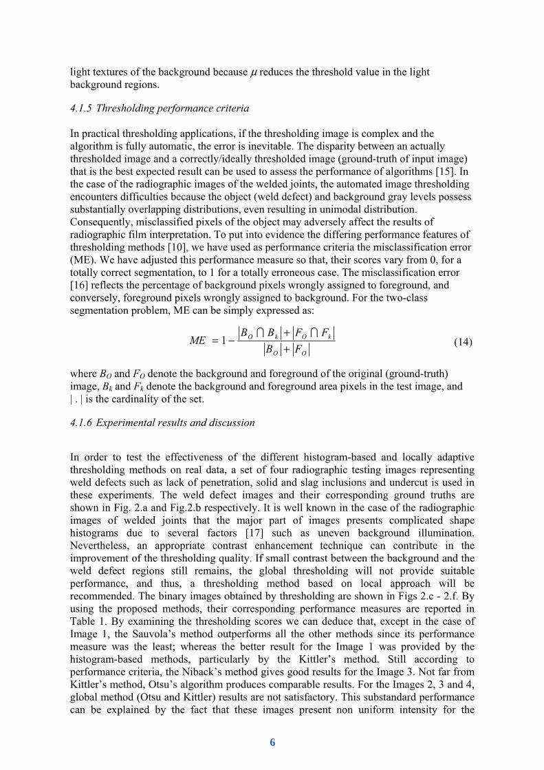
In order to test the effectiveness of the different histogram-based and locally adaptive thresholding methods on real data, a set of four radiographic testing images representing weld defects such as lack of penetration, solid and slag inclusions and undercut is used in these experiments. The weld defect images and their corresponding ground truths are shown in Fig. 2.a and Fig.2.b respectively. It is well known in the case of the radiographic images of welded joints that the major part of images presents complicated shape histograms due to several factors [17] such as uneven background illumination. Nevertheless, an appropriate contrast enhancement technique can contribute in the improvement of the thresholding quality. If small contrast between the background and the weld defect regions still remains, the global thresholding will not provide suitable performance, and thus, a thresholding method based on local approach will be recommended. The binary images obtained by thresholding are shown in Figs 2.c - 2.f. By using the proposed methods, their corresponding performance measures are reported in Table 1. By examining the thresholding scores we can deduce that, except in the case of Image 1, the Sauvola’s method outperforms all the other methods since its performance measure was the least; whereas the better result for the Image 1 was provided by the histogram-based methods, particularly by the Kittler’s method. Still according to performance criteria, the Niback’s method gives good results for the Image 3. Not far from Kittler’s method, Otsu’s algorithm produces comparable results. For the Images 2, 3 and 4, global method (Otsu and Kittler) results are not satisfactory. This substandard performance can be explained by the fact that these images present non uniform intensity for the

6

background which confounds in some areas with the defect region. For example, the weld defect (external undercut) presented in the Image 4 is totally drowned in the background by the Otsu’s and Kittler’s methods, which affects dangerously the interpretation results.

Fig. 2 Thresholding results of weld radiographic images (a) Weld defect images. (b) Ground-truths of a. (c) Otsu’s thresholding.

(d) Kittler’s thresholding (e) Niblack’s thresholding. (f) Sauvola’s thresholding.

Table 1 Misclassification error measures For the Niblack and Sauvola methods, the values of W=13, k (Nib.)=−0.2, k(Sauv.) = 0.5 and R=128 are selected. This choice was made in an empirical way, taking in account the dilemma between robustness (non sensitiveness to noise) and precision (space definition of the segmented areas).

4.1.7 Post-processing and morphological operations

After the thresholding stage, the binary image can contain: • superfluous information that it is suitable to eliminate, • or masked information that it is necessary to reveal and this, whatever the employed

thresholding method. The processing based on mathematical morphology makes possible to modify the

binary image for this purpose. Dilatations and erosions are often used in pairs to obtain morphological opening and closing. Opening by a disk structuring element smoothes the

Otsu Kittler Niblack Sauvola

Image 1 0.0774 0.0425 0.1441 0.1587

Image 2 0.5453 0.4433 0.2582 0.0452

Image 3 0.4363 0.4299 0.1675 0.1568

Image 4 0.6297 0.4777 0.1060 0.0444

a.

b.

c.

d.

e.

f.

Image 1 Image 2 Image 3 Image 4

7

boundary, breaks narrow parts, and eliminates small objects. Closing by a disk structuring element smoothes the boundary, fills narrow bays, and eliminates small holes.

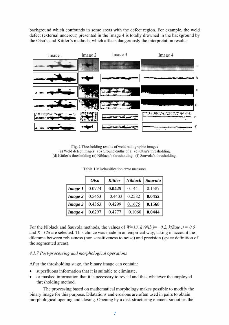
By referring to morphological operators properties [18], it thus becomes convenient to apply these operators like their combination in order to eliminate the noise and the small residual spots in the thresholded image. We must consider that at the end of this stage, we obtain only one connected region which represents the more accurately possible, the weld defect and on which we extract various features necessary to the classification stage. The combination of the median filter with the morphological operators of dilation, erosion, opening and closing allows us: to remove the noise, to eliminate the small residual spots and to connect closed regions likely to represent the same weld defect.

a. b.

Fig. 3 Examples of the application of morphological filtering on radiographic binary images

In Fig. 3.a, one pass of median filter on the Sauvola thresholded image followed by

an opening/closing using square structuring element (2×2 of ones) is sufficient to obtain the expected result. On the other hand, in the case of Fig. 3.b, it was necessary to apply two passes of median filtering, followed by double dilation and double erosion using a rectangular structuring element (2×3 of ones). This choice is justified by the fact that in this last case, the structuring element must play a double role: eliminate the small irrelevant areas and connect regions which belong a priori to the same region representing the weld defect.

4.2 Contour estimation based maximum likelihood

Many works have been proposed about the active contour models in the different fields especially in medical imaging [19], [20], [21] and so on. In this section, we describe a new method for automatic estimation of weld defect contours in radiographic images. To deal with the low quality of radiography images, we describe the contour shapes using low order parametric deformable models. This low-order parameterization is sufficient to accommodate the expected shape and size variations, yet provides robustness against noise, image artifacts and regions of missing data. The problem is formulated in a statistical estimation framework, and implementation is carried out by unsupervised deterministic iterative algorithms.

4.2.1 Problem formulation

A. Probabilistic Image Model: Our approach consists of a maximum likelihood estimation approach to parametric deformable models. The basic building block is a probabilistic observation model ( )θ/ZP characterizing the observed data Z given the parameter vector θ which describes the contour shape. Under the maximum likelihood (ML) criterion, the best estimate of θ denoted by MLθ̂ , ML is given by

( )( )θθθ

/maxargˆ ZpML = (15)

8

To derive the likelihood function ( )θ/Zp , we adopt a region based approach; this has been shown to provide robustness with respect to local artifacts and poor image quality, [21]. In our region-based model, Z consists of all the image data, thus being less sensitive to noise and image artifacts than methods that use local derived information (such as gradients or edges) . In particular, we consider a simple model in which the image is divided into two regions, inside and outside, separated by the boundary to be estimated. The observed image Z (an array of gray levels), is modelled as a random function of the object's boundary curve ( )θv , which is a function of the unknown parametersθ . Moreover, Z may also depend on some additional observation parametersφ . Accordingly, our likelihood function can be written as ( )φθ ,/Zp .

The simplest possible region-based model is characterized by the two following hypotheses: conditional independence (given the region boundary, all the pixels are independent); and region homogeneity (the probability distribution of each pixel only depends on whether is belongs to the inside or outside region). Thus, the likelihood function can be written as

( ) ( )( )( )

( )( )( )

∏∏∈∈

×=θθ

φφφθvOji

outjivIji

inji ZpZpZp),(

),(),(

),( //,/ (16)

with ( )jiZ , denoting the value of pixel ( )ji, , while ( )( )θvI and ( )( )θvO are, respectively, the inside and outside regions of the contour ( )θv . Finally, ( )( )injiZp φ/, and ( )( )outjiZp φ/, are the pixel-wise probability functions of these two regions.

Given that radiography images are well described by Rayleigh or Gaussian distributions, Rayleigh density has the form:

( ) ⎟⎟⎠

⎞⎜⎜⎝

⎛−=

φφφ

2exp/

2xxxp (17)

and thus [ ]outin φφφ ,= , where inφ and outφ are the variances for the inside and outside regions, respectively. Gaussian density has the form:

( )⎥⎥⎦

⎤

⎢⎢⎣

⎡⎟⎟⎠

⎞⎜⎜⎝

⎛ −−=2

2exp

21/

σμ

πσφ xxp (18)

and thus [ ]σμφ ,= with [ ]outin μμμ ,= ,where inμ and outμ are the means for the inside and outside regions, respectively. [ ]outin σσσ ,= , where inσ and outσ are the standard deviations for the inside and outside regions, respectively. B. Complete Estimation Criterion and Algorithm: To obtain an unsupervised scheme, we must estimate, from an observed image Z, not only the parameters that define the contour,θ , but also the other parameters . Accordingly, we extend the maximum likelihood criterion to include also these parameters:

( ) ( )( )φθφθφθ

,/maxargˆ,ˆ,

Zp= (19)

Since solving (19) simultaneously with respect to θ and φ would be computationally very difficult, we settle for a suboptimal solution given by iterative schemes of the type

9

( ) ( )( )( )tt Zp φθθθ

ˆ,/maxargˆ 1 =+ (20)

( ) ( )( )( )φθφφ

,ˆ/maxargˆ 11 ++ = tt Zp (21)

where ( )tθ̂ and ( )tφ̂ are the estimates of θ and φ at iteration t, respectively [21].

4.2.2 Results and Discussion

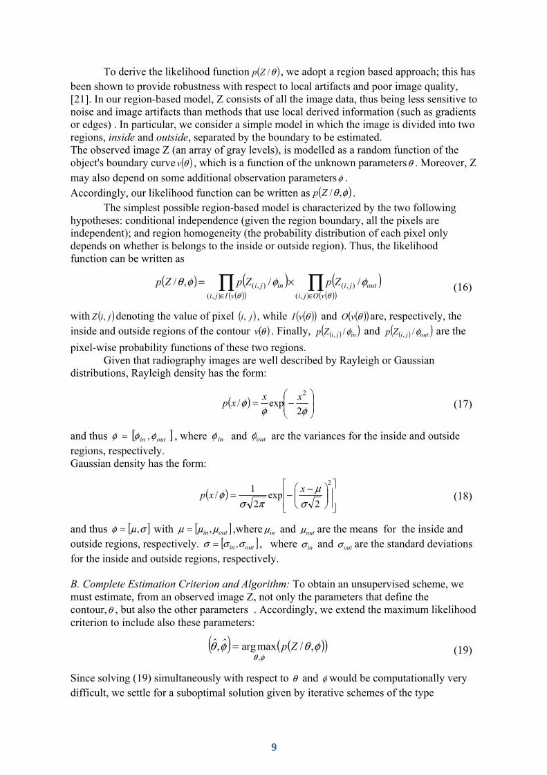
We have implemented two contour estimation algorithms: one with Raleigh distribution, and another with Gaussian distribution. In both cases, the underlying criterion and type of algorithm are those in (19), (20), and (21). The first two examples simply illustrate the results of the algorithm using synthetic images generated according to the Rayleigh and Gaussian models. In Fig. 4, we simulate a weld defect by Gaussian model, with the inner and outer parameters set to ( )3,80 == inin σμ and ( )4,150 == outout σμ respectively. The final parameter estimates are ( )91.2ˆ,55.81ˆ == inin σμ and ( )15.4ˆ,67.148ˆ == outout σμ . In the example of Fig. 5, we simulate a weld defect by Raleigh model, with the inner and outer variances set to 80 and 150, respectively. The image model parameter estimates obtained were 65.80ˆ =inφ and 26.151ˆ =outφ .

In the final example shown in Fig. 6, we employ our method to extract the defect contour from the radiographic image with Rayleigh model. The left image in Fig. 6 shows the selected initial contour. We can see the initial contour is far from the reel one. The middle image in Fig. 6 is obtained after some iterations, we remark that the selected contour come close to the defect one. Finally, in the right image in Fig. 6, the deformable contour is closed-fitting to the defect edge.

Fig. 4 Synthetic image with Gaussian model: initial contour, intermediate contours and final contour

Fig. 5 Synthetic image with Raleigh model: initial contour, intermediate contours and final contour

Fig. 6 Real image of weld defect with Raleigh model: initial contour, intermediate contour and final contour.

10

5. Feature extraction and selection

5.1 Invariant attributes calculation

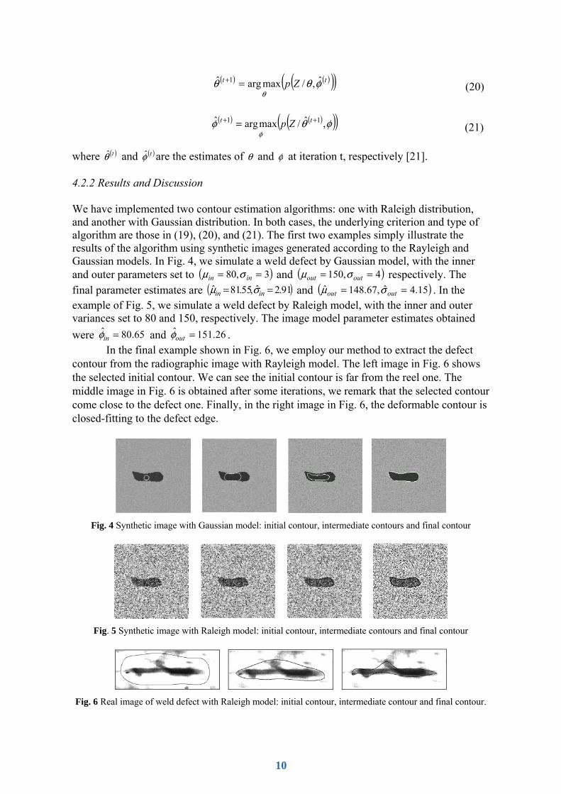
After each weld defect is isolated, its geometric parameters: Area (A), perimeter (P) [22], centre of gravity ),( yxG , angle of orientation (α), principal axes of inertia, width (W) and length (L) of the minimal surrounding rectangle, maximal diameter (Dmax), radius of maximal inscribed circle (Rmax), semi major and semi-minor axes (a,b) of the image ellipse (see Fig. 7) are computed.

Fig. 7 Illustration of the geometric parameters

The geometric attributes which we will define below are invariants regardless geometric transformations of translation, rotation and scaling.

Compactness 2PA4Comp /π= (22)

Elongation WLElong /= (23)

Rectangularity )./( WLARct = (24)

Anisometry baAni /= (25)

Symmetry SymVSymHSym ×= (26)

where SymV and SymH are given by the algorithm : if (S4+S3)<(S1+S2) then SymV=(S4+S3)/(S1+S2); else SymV=(S1+S2)/(S4+S3); if (S2+S3)<(S1+S4) then SymH=(S2+S3)/(S1+S4); else SymH=(S1+S4)/(S2+S3);

Lengthening index A4DI 2a /max×= π (27)

Center of gravity

G

α Surrounding rectangle

Inscribed maximal circle

Maximal diameter

First principal axis

S3

S2

S4

S1

Image ellipse

11

Deviation index to inscribed circle ARI r /1 2

maxπ−= (28)

Invariant moments ( )⎪⎩

⎪⎨⎧

+−=Φ

+=Φ2

112

02202

02201

4ηηη

ηη (29)

where 2qp100pqpq

/)( ++= μμη p+q = 2,3,...

are the normalized central moments [23] and

( ) ( )( )( )( ) ( ) ⎥

⎥⎦

⎤

⎢⎢⎣

⎡

−=−−=−

−−=−−=

∑∑∑∑

n

i iin

i i

in

i in

i i

yyyyxx

yyxxxx2

2,01,1

1,12

0,2

μμμμ

(30)

is the covariance matrix of the object.

Because the different raw geometric attributes have values ranging from the order of 0 to 200, the features were rescaled to lie between 0 and 1, to avoid the effects of the larger features “swamping” those of the smaller features and possible numerical errors caused by a large range in values [24]. 5.2 Relationship between the proposed attributes and the weld defect types Compactness (Comp): Its value is included in [0,1]. It has little values for sharp defects (crack, lack of fusion) and it has values near to 1 for spherical defects (porosity, tungsten inclusion, etc.). Elongation (Elong): It describes the occupied area in the bounding box of defect. Big values of this attribute characterize longitudinal defects (crack, lack of fusion, lack of penetration, elongated porosity, undercut, etc.). Rectangularity (Rect): Its value is included in [0,1]. It is equal to 1 for a rectangle. It characterizes rectangular defects (lack of penetration). Anisometry (Ani): It depends on the direction of principal axis of defect. Its value is proportional to defect lengthening. Symmetry (Sym): Its value is included in [0,1]. The value 1 describes a perfectly symmetrical shape. Asymmetrical aspects of defects (slag inclusion, warm holes, etc.) are related by little values of this attribute. Lengthening index (Ia): Big values of this indicia put in obviousness fine and rectilinear cracks. Deviation index to inscribed circle (Ir): The indicia value is maximal (near to 1) for lengthened defects and minimal (near to 0) for round defects. Invariant moments (Φ1,Φ2): They gives measures in relation with the pixel spreading in comparison with the centre of mass.

5.3 Principal Component Analysis (PCA) for feature selection

In order to reduce the computational time required for the classification stage it is necessary to select attributes; thus the classifier only works with non-correlated attributes that provide defect detection information. There are a variety of methods for evaluating the performance of the computed attributes.

In our study, we investigate the use of PCA relevant features from the feature vector. This technique is widely used in many areas of applied statistics. It is natural since

12

interpretation and visualization in a fewer dimensional space is easier than in many dimensional space [25]. PCA is a statistical tool, which is useful to extract dominant features (principal components) from the set multivariate data. They explain the maximum amount of variance possible by linear transforms by projecting the data into orthonormal sub-spaces. In our case, PCA will enable us to reduce the dimension of the feature vector and the extracted features should contain the most relevant information.

The initial data can be represented by a matrix with M attribute variables and N individuals (defects). We will have an array matrix Γ with the size of N×M. Therefore, we have

[ ]M21 ΓΓΓ=Γ ,,, L (31)

The mean of the column vector i is defined by:

∑=

Γ=ΨN

n

ni N1

1 (32)

The subtracted training set is represented as matrix:

[ ]MΦΦΦ=Φ ,,, 21 L with iii Ψ−Γ=Φ (33)

The covariance matrix is calculated using

TC ΦΦ= (34)

The eigenvector of matrix C as ivr with corresponding eigenvalues can be computed by

iii vvC rr λ= (1 ≤ i ≤ L ≤ M) (35)

Any weld defect can be identified as a linear combination of the eigenvectors. The principal components for any weld defect are defined by:

[ ]TL

T2

T1 vvvP

rL

rr,,,Γ= (36)

The matrix P with the size of N×L represents the database into the axis corresponding to the eigenvector. The values of this matrix are the new features that can be used for classification and recognition purposes.

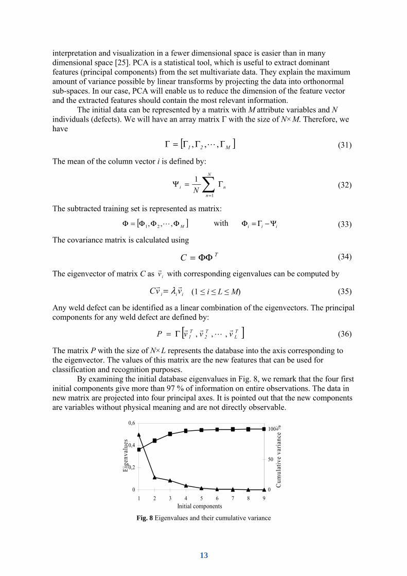
By examining the initial database eigenvalues in Fig. 8, we remark that the four first initial components give more than 97 % of information on entire observations. The data in new matrix are projected into four principal axes. It is pointed out that the new components are variables without physical meaning and are not directly observable.

0

0,2

0,4

0,6

1 2 3 4 5 6 7 8 9Initial components

Eige

nval

ues

0

50

100

Cum

ulat

ive

varia

nce

%

Fig. 8 Eigenvalues and their cumulative variance

13

6. Weld defect classification

6.1 EM algorithm for mixture models

Consider mixture model with M components or classes (M>1) in ℜn for n≥1.

( ) ( )∑=

=M

mm mxpxp

1

/α (37)

where [ ]1 , 0∈mα (m = 1,2 … M) are the mixing proportions subject to

11

=∑=

M

mmα (38)

For Gaussian mixtures, each component density )/( mxp is a normal probability distribution:

⎥⎦⎤

⎢⎣⎡ −−−= −

)1

2/12/ ()(21exp

)det()2(1)/( mm

Tm

mnm xCx

Cxp μμ

πθ (39)

where T denotes the transpose operation. Here we encapsulate these parameters into parameter vector, writing the parameters of each component as )( , mmm Cμθ = (μm and Cm

represent respectively the mean and the covariance matrix of the class m) to get mααα ,...,,( 21=Θ ),......,, 21 mθθθ then (37) can be rewritten as

( ) ( )∑=

=ΘM

mmm xpxp

1

// θα (40)

If we knew the component from which x came, then it would be simple to determine the parameters Θ . Similarly, if we knew the parameter Θ , we could determine the component that would be most likely to have produced x. The difficulty is that we know neither. However, the EM algorithm could be introduced to deal with this difficulty through the concept of missing [26]. EM algorithm is a widely used class of iterative algorithms for maximum likelihood (ML) or maximum posteriori (MAP) estimation in problems with missing data. Given a set of samples X=(x1,x2,...,xk), the complete data set Z=(X, Y) consists of the sample set X and a set Y of variables indicating from which component of the mixtures the sample came. Now, we discuss how to estimate the parameters of the Gaussian mixtures with the EM algorithm [27].

The EM algorithm consists of an E-step and M-step. Suppose that )(tΘ denotes the estimation of Θ obtained after the tth iteration of the algorithm. Then at the (t+1)th iteration, the E-step computes the expected complete data log-likelihood function

( ) ( ){ } ( )∑∑= =

Θ=ΘΘK

k

M

m

tkmkm

t xmPxpQ1 1

)()( ;//log/ θα (41)

where ( ))(;/ tkxmP Θ is a posterior probability and is computed as

( )( )∑

=

=Θ M

l

tlk

tm

tmk

tmt

k

xp

xpxmP

1

)()(

)()()(

/

)/(;/θα

θα (42)

14

And the M-step finds the (t+1)th estimation )1( +Θ t of Θ by maximizing ( ))(/ tQ ΘΘ

( )∑=

+ Θ=K

k

tk

tm xmP

K 1

)()1( ;/1α (43)

( )

( )∑

∑

=

=+

Θ

Θ= K

k

tk

K

k

tkk

tm

xmP

xmPx

1

)(

1

)(

)1(

;/

;/μ (44)

( ) ( )( )

( )∑

∑

=

=

++

+

Θ

⎭⎬⎫

⎩⎨⎧ −−Θ

= K

k

tk

K

k

Ttmk

tmk

tk

tm

xmP

xxxmPC

1

)(

1

)1()1()(

)1(

;/

;/ μμ (45)

6.2 Choice of the weld defect categories

By examining number of radiographic films and according to morphological characteristics of weld defects, we can deduce four principal shape categories: First category: The defects of which the shape is lengthened, sharp and rectilinear (cracks, undercut, lateral lack of fusion, etc.). Second category: The defects of which the shape is lengthened, smooth and rectangular (lack of penetration, elongated porosities, etc.). Third category: The defects with spherical shape (porosities, tungsten inclusions, etc.). Fourth category: The defects with irregular shape (non lengthened and non spherical) (solid inclusions, slag inclusions, worm holes, etc.).

6.3 Artificial Neural Network (ANN) and its configuration for weld defect classification

A feed forward neural network trained by the backpropagation algorithm [28] is used for the weld defect classification task [29], [30]. This neuronal classification consists in assigning the usual types of weld defects met in practice to four categories described above. Thus, we introduce as input data of ANN the four principal components obtained in § 5.3.

15

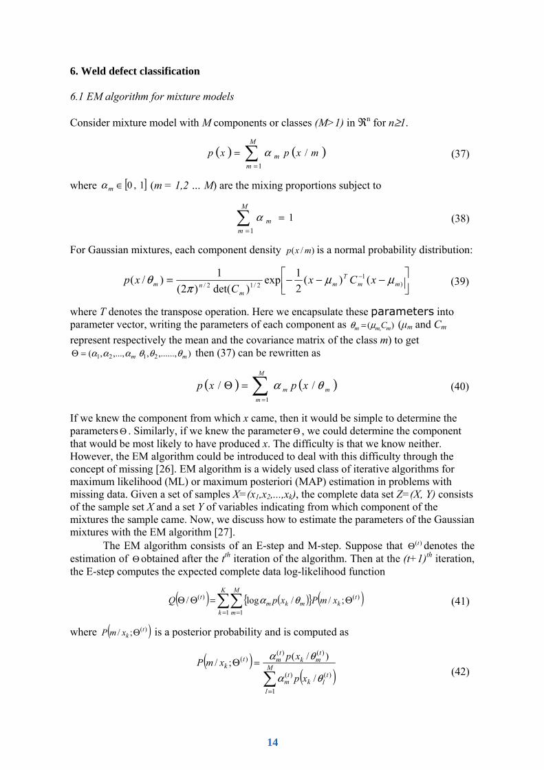
Fig. 9 Configuration of the used neural network

As shown in Fig. 9, four neurons in the output layer correspond, each one to a defect category. Initially, the network is trained with the principal component vectors, and their corresponding weld defect categories. Each defect category is assigned to a distinct output class. A first set of weld defects is used as learning data in training by backpropagation. The test set is made up on non learned or unknown defects.

6.4 Experiments and discussion

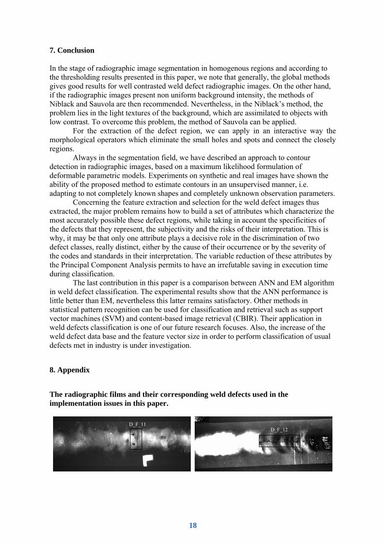
Some defects extracted from the weld defect database are chosen to constitute the training data for ANN classifier. For the testing step, we present to the neural network a set of non learned (unknown) radiographic images of weld defects shown in Appendix. First, to make the ground truth, we have assigned to each category a number of weld defects from the testing set by taking into account the opinion of the radiograph interpreter. Therefore, a test is conclusive if the result of the classification of the non learned defect corresponds to the class predefined by the radiograph expert.

The test results (see Table 2) show us that almost the entire defects presented to ANN correspond to interpretations emitted a priori by the experts, with a precision exceeding 95% (except Df_45 with 67%). By examining the shape of Df_12, we can remark that its relatively important width with its pronounced asymmetric shape can relatively move it away from the category C1 and bring it to the category C4. We can also remark that the defect Df_44 is classified with the accuracy of 99.60% in the category C4 predefined by radiograph, nevertheless the ANN classifies it in the same time to the category C2 with a precision of 40%. This can be justifiable in taking in account the defect shape which can be characterized by certain rectangularity. This last is a decisive attribute for the category C2.

Only one defect Df_23, defined by the experts as being a lack of penetration i.e. belonging to category C2, was classified by the neuronal classifier in the category C1 i.e. in the category corresponding to cracks, undercut etc. In fact, the more discriminating attribute between these two classes is the rectangularity. The category C1 is characterized by a weak rectangularity and inversely for C2. For this defect image, the circular shape in its right side and the gradual erosion of its surface influence considerably, among other things, its rectangularity. This shape can be caused by the presence of another weld defect (burn through) and the geometrical blur aspect due the radiographic exposure process. These

⎥⎥⎥⎥

⎦

⎤

⎢⎢⎢⎢

⎣

⎡

Γ

4Comp3Comp2Comp1Comp

ACP

C1 C2 C3 C4

1 0 0 0

0 1 0 0

0 0 1 0

0 0 0 1

T r a i n i n g d a t a s e t

T e s t i n g d a t a s e t

16

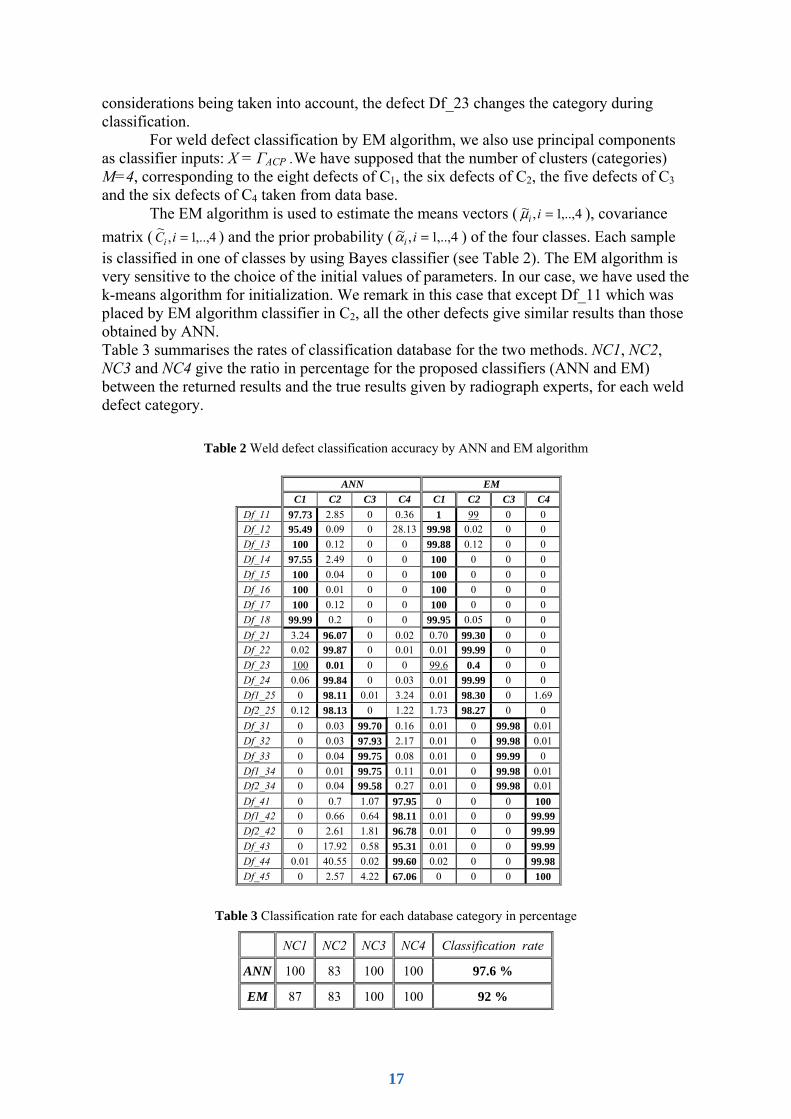
considerations being taken into account, the defect Df_23 changes the category during classification.

For weld defect classification by EM algorithm, we also use principal components as classifier inputs: X = ΓACP .We have supposed that the number of clusters (categories) M=4, corresponding to the eight defects of C1, the six defects of C2, the five defects of C3 and the six defects of C4 taken from data base.

The EM algorithm is used to estimate the means vectors ( 4,..,1,~ =iiμ ), covariance matrix ( 4,..,1,~ =iCi ) and the prior probability ( 4,..,1,~ =iiα ) of the four classes. Each sample is classified in one of classes by using Bayes classifier (see Table 2). The EM algorithm is very sensitive to the choice of the initial values of parameters. In our case, we have used the k-means algorithm for initialization. We remark in this case that except Df_11 which was placed by EM algorithm classifier in C2, all the other defects give similar results than those obtained by ANN. Table 3 summarises the rates of classification database for the two methods. NC1, NC2, NC3 and NC4 give the ratio in percentage for the proposed classifiers (ANN and EM) between the returned results and the true results given by radiograph experts, for each weld defect category.

Table 2 Weld defect classification accuracy by ANN and EM algorithm

Table 3 Classification rate for each database category in percentage

NC1 NC2 NC3 NC4 Classification rate

ANN 100 83 100 100 97.6 %

EM 87 83 100 100 92 %

ANN EM C1 C2 C3 C4 C1 C2 C3 C4

Df_11 97.73 2.85 0 0.36 1 99 0 0 Df_12 95.49 0.09 0 28.13 99.98 0.02 0 0 Df_13 100 0.12 0 0 99.88 0.12 0 0 Df_14 97.55 2.49 0 0 100 0 0 0 Df_15 100 0.04 0 0 100 0 0 0 Df_16 100 0.01 0 0 100 0 0 0 Df_17 100 0.12 0 0 100 0 0 0 Df_18 99.99 0.2 0 0 99.95 0.05 0 0 Df_21 3.24 96.07 0 0.02 0.70 99.30 0 0 Df_22 0.02 99.87 0 0.01 0.01 99.99 0 0 Df_23 100 0.01 0 0 99.6 0.4 0 0 Df_24 0.06 99.84 0 0.03 0.01 99.99 0 0 Df1_25 0 98.11 0.01 3.24 0.01 98.30 0 1.69 Df2_25 0.12 98.13 0 1.22 1.73 98.27 0 0 Df_31 0 0.03 99.70 0.16 0.01 0 99.98 0.01 Df_32 0 0.03 97.93 2.17 0.01 0 99.98 0.01 Df_33 0 0.04 99.75 0.08 0.01 0 99.99 0 Df1_34 0 0.01 99.75 0.11 0.01 0 99.98 0.01 Df2_34 0 0.04 99.58 0.27 0.01 0 99.98 0.01 Df_41 0 0.7 1.07 97.95 0 0 0 100 Df1_42 0 0.66 0.64 98.11 0.01 0 0 99.99Df2_42 0 2.61 1.81 96.78 0.01 0 0 99.99Df_43 0 17.92 0.58 95.31 0.01 0 0 99.99Df_44 0.01 40.55 0.02 99.60 0.02 0 0 99.98Df_45 0 2.57 4.22 67.06 0 0 0 100

17

7. Conclusion

In the stage of radiographic image segmentation in homogenous regions and according to the thresholding results presented in this paper, we note that generally, the global methods gives good results for well contrasted weld defect radiographic images. On the other hand, if the radiographic images present non uniform background intensity, the methods of Niblack and Sauvola are then recommended. Nevertheless, in the Niblack’s method, the problem lies in the light textures of the background, which are assimilated to objects with low contrast. To overcome this problem, the method of Sauvola can be applied.

For the extraction of the defect region, we can apply in an interactive way the morphological operators which eliminate the small holes and spots and connect the closely regions.

Always in the segmentation field, we have described an approach to contour detection in radiographic images, based on a maximum likelihood formulation of deformable parametric models. Experiments on synthetic and real images have shown the ability of the proposed method to estimate contours in an unsupervised manner, i.e. adapting to not completely known shapes and completely unknown observation parameters.

Concerning the feature extraction and selection for the weld defect images thus extracted, the major problem remains how to build a set of attributes which characterize the most accurately possible these defect regions, while taking in account the specificities of the defects that they represent, the subjectivity and the risks of their interpretation. This is why, it may be that only one attribute plays a decisive role in the discrimination of two defect classes, really distinct, either by the cause of their occurrence or by the severity of the codes and standards in their interpretation. The variable reduction of these attributes by the Principal Component Analysis permits to have an irrefutable saving in execution time during classification.

The last contribution in this paper is a comparison between ANN and EM algorithm in weld defect classification. The experimental results show that the ANN performance is little better than EM, nevertheless this latter remains satisfactory. Other methods in statistical pattern recognition can be used for classification and retrieval such as support vector machines (SVM) and content-based image retrieval (CBIR). Their application in weld defects classification is one of our future research focuses. Also, the increase of the weld defect data base and the feature vector size in order to perform classification of usual defects met in industry is under investigation.

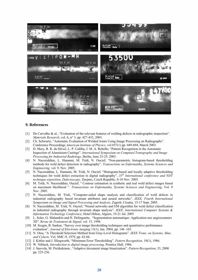
8. Appendix

The radiographic films and their corresponding weld defects used in the implementation issues in this paper.

D_F_12 D_F_11

18

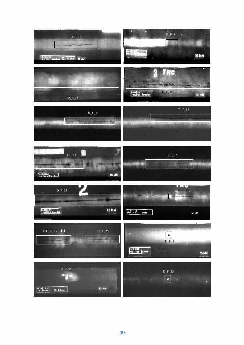
D_F_13 D_F_14

D_F_15

D_F_16

D_F_17 D_F_18

D_F_21 D_F_22

D_F_23 D_F_24

D1_F_25 D2_F_25

D_F_31

D_F_32 D_F_33

19

9. References

[1] De Carvalho & al., “Evaluation of the relevant features of welding defects in radiographic inspection”. Materials Research, vol. 6, n° 3, pp. 427-432, 2003.

[2] Ch. Schwartz, “Automatic Evaluation of Welded Joints Using Image Processing on Radiographs”. Conference Proceedings American Institute of Physics, vol 657(1) pp. 689-694, March 2003.

[3] D. Mery, R. R. da Silva2, L. P. Calôba, J. M. A. Rebello, “Pattern Recognition in the Automatic Inspection of Aluminium Castings”. International Symposium on Computed Tomography and Image Processing for Industrial Radiology, Berlin, June 23-25, 2003.

[4] N. Nacereddine, L. Hamami, M. Tridi, N. Oucief, “Non-parametric histogram-based thresholding methods for weld defect detection in radiography”. Transactions on Enformatika, Systems Sciences and Engineering, vol. 9, Nov. 2005.

[5] N. Nacereddine, L. Hamami, M. Tridi, N. Oucief, “Histogram-based and locally adaptive thresholding techniques for weld defect extraction in digital radiography”. 35th International conference and NDT technique exposition, Defectoscopy, Znojmo, Czech Republic, 8-10 Nov. 2005.

[6] M. Tridi, N. Nacereddine, Oucief, “ Contour estimation in synthetic and real weld defect images based on maximum likelihood ”. Transactions on Enformatika, Systems Sciences and Engineering, Vol. 9 Nov. 2005.

[7] N. Nacereddine, M. Tridi, “Computer-aided shape analysis and classification of weld defects in industrial radiography based invariant attributes and neural networks”. IEEE, Fourth International Symposium on Image and Signal Processing and Analysis, Zagreb, Croatia, 15-17 Sept. 2005.

[8] N. Nacereddine, M. Tridi, N. Oucief, “Neural networks and EM algorithm for weld defect classification in industrial radiography through invariant shape analysis”. IEEE, International Computer Systems & Information Technology Conference, Hotel Hilton, Algiers, 19-21 Jul. 2005

[9] L. Soler, G. Malandrin and H. Delinguette, “Segmentation automatique: Application aux angioscanners 3D”. Revue de Traitement de Signal, vol. 15, 1998.

[10] M. Sezgin, B. Sankur, “Survey over image thresholding techniques and quantitative performance evaluation”. Journal of Electronic imaging 13(1), Jan. 2004, pp. 146–165.

[11] N. Otsu, “A Threshold Selection Method from Gray-Level Histograms”. IEEE Trans. on Systems, Man, and Cybern, Vol. SMC-9, 1979, pp. 62-66.

[12] J. Kittler and J. Illingworth, “Minimum Error Thresholding”. Pattern Recognition, 19(1), 1986. [13] W. Niblack, Introduction to digital image processing. Prentice Hall, 1986. [14] J. Sauvola, M. Pietikakinen , “Adaptive document image binarization”. Pattern Recognition, 33, 2000

pp. 225-236.

D2_F_34

D1_F_34 D_F_41

D1_F_42 D2_F_42 D_F_43

D_F_44 D_F_45

20

[15] Y. J. Zhang, “A survey on evaluation methods for image segmentation”. Pattern Recognition, 29(8),1996.

[16] W. A. Yasnoff, J. K. Mui, and J. W. Bacus, “Error measures for scene segmentation”. Pattern Recognition, 9, 1977, pp. 217–231.

[17] N. Nacereddine, “Weld defect detection and recognition in industrial radiography based image analysis and neuronal classifiers”. Fourth International Conference on NDE in Relation to Structural Integrity for Nuclear and Pressurised Components, London, 6-8 Dec. 2004

[18] R.M. Haralick, S.R. Sternberg, X. Zhuang, “Image analysis using mathematical morphology”. IEEE Trans on Pattern Analysis And Machine Intelligence, vol.9/4, pp.532-550, 1987.

[19] M. Figueiredo and J. Leitão, “.Bayesian estimation of ventricular contours in angiographic images”. IEEE Trans. on Medical Imaging, vol. 11, no. 3, 1992, pp. 416-429.

[20] M. Figueiredo, J. Leitão, and A. K. Jain, “Unsupervised contour representation and estimation using B-splines and a minimum description length criterion”. IEEE Trans. on Image Processing, vol. 9, 2000, pp. 1075-1087

[21] S. V. B. Jardim and M. Figueiredo, “automatic contour estimation in fetal ultrasound images”. Proc. International Conference on Image Processing (ICIP’03), Barcelona, Spain, Sept. 2003.

[22] L. Dorst and A.W.M. Smeulders, “Length Estimators for Digitized Contours”. Computer Vision, Graphics and Image Processing, vol. 40, pp.311−333, 1987.

[23] M.K. Hu, “Visual Pattern Recognition by Moments Invariants”. IRE Trans. Info. Theory, vol. IT-8, 1962.

[24] N. Nacereddine, “Automated method implementation for detection and classification of weld defects in industrial radiography”. M.S. thesis, Dept. Automation, Boumerdes Univ., Algeria, Jul. 2004.

[25] A.K. Jain, P.W. Duin & Jianchang Mao, “Statistical Pattern Recognition: A Review”. IEEE Trans on Pattern Recognition analysis and machine intelligence, Vol 22, No 1, January 2000.

[26] Z. Baibo, Z. Changshui, “Competitive EM algorithm for finite mixture models”. Pattern Recognition 37, 2004, pp. 131-144.

[27] Z. Zhihua, C. Chen, “EM algorithms for Gaussian mixtures with split and merge operation”. Pattern Recognition 36, 2003, pp 1973-1983.

[28] H.D. Cheng and al. “Computer-aided detection and classification of microcalcifications in mammography: a survey”. Pattern recognition, (36)12, pp. 2967-2991, 2003.

[29] R.P. Lippmann, “An introduction to computing with neural nets”. IEEE ASSP Magazine. 1987. [30] N. Nacereddine, R. Drai, A. Benchaâla, “Weld defect Extraction and Classification in radiographic

testing based Artificial Neural Networks”. 15th World Conference on non-destructive Testing, Roma, Italy, 15-21 Oct. 2000.

21