Statistical Profile Estimation in Database Systemspeople.csail.mit.edu/tdanford/6830papers/mannino-stat-profile-estimation.pdfStatistical Profile Estimation in Database Systems

Statistical Profile Estimation in Database Systems

MICHAEL V. MANNINO

Department of Manugement Science and Information Systems, University of Texas at Austin, Austin, Texas 78712

PAICHENG CHU

Department of Accounting and Management Inform&ion Systems, Ohio State University, Columbus, Ohio 43210

THOMAS SAGER

Department of Management Science and Information Systems, University of Texas at Austin, Austin, Texas 78712

A statistical profile summarizes the instances of a database. It describes aspects such as the number of tuples, the number of values, the distribution of values, the correlation between value sets, and the distribution of tuples among secondary storage units. Estimation of database profiles is critical in the problems of query optimization, physical database design, and database performance prediction. This paper describes a model of a database of profile, relates this model to estimating the cost of database operations, and surveys methods of estimating profiles. The operators and objects in the model include build profile, estimate profile, and update profile. The estimate operator is classified by the relational algebra operator (select, project, join), the property to be estimated (cardinality, distribution of values, and other parameters), and the underlying method (parametric, nonparametric, and ad-hoc). The accuracy, overhead, and assumptions of methods are discussed in detail. Relevant research in both the database and the statistics disciplines is incorporated in the detailed discussion.

Categories and Subject Descriptors: H.0 [Information Systems]: General; H.2.2 [Database Management]: Physical Design--access methods; H.2.3 [Database Management]: Languages-query languages; H.2.4 [Database Management]: Systems-query processing; H.3.3 [Information Storage and Retrieval]: Information Search and Retrieval-query formulution; retrieval models; search process; selection process

General Terms: Algorithms, Languages, Performance

Additional Key Words and Phrases: Access plan, Boolean expressions, database profile, relational model

INTRODUCTION an integral element of the optimizing component in query optimization and, in some

The quantitative properties that summa- cases, physical database design. rize the instances of a database are its The objective of query optimization is to statistical profile. Estimation of profiles is derive an efficient plan for obtaining the

Permission to copy without fee all or part of this material is granted provided that the copies are not made or distributed for direct commercial advantage, the ACM copyright notice and the title of the publication and its date appear, and notice is given that copying is by permission of the Association for Computing Machinery. To copy otherwise, or to republish, requires a fee and/or specific permission. 0 1988 ACM 0360-03OO/SS/O900-0191$01.50

ACM Computing Surveys, Vol. 20, No. 3 September 1988

192 l M. V. Mannino et al.

CONTENTS

INTRODUCTION 1. DATABASE PROFILE AS A COMPLEX

OBJECT 2. RELATIONSHIP BETWEEN PROFILE AND

COST ESTIMATION 2.1 Basics of Cost Estimation 2.2 Example Cost Extimatas 2.3 Sensitivity Analysis

3. PRIMER ON STATISTICAL METHODS 3.1 Common Parametric Distributions 3.2 Nonparametric Estimation

4. ESTIMATION OF SINGLE OPERATIONS 4.1 Select 4.2 Project 4.3 Join 4.4 Set Operators 4.5 Summary

5. ESTIMATION OF MULTIPLE OPERATIONS 5.1 Projections after Selections and Joins 5.2 Joins after Selections

6. FUTURE DIRECTIONS 7. CONCLUSION ACKNOWLEDGMENTS REFERENCES

information requested by the user. A plan is a high-level description of a program. It describes the algorithms, file structures, order of operations, and outer/inner loop variables. To find an efficient plan, an optimizer generates and evaluates a number of alternatives. The evaluation of alternatives is based on cost formulas that estimate the number of secondary storage accesses, the central processing effort, and in the case of distributed databases, the communication costs and delays. Since these formulas depend directly or indirectly on the estimated size of the operands, statistical profile estimation assumes importance in the process of query optimization.

Statistical profile estimation can also play an important role in physical database design problems such as index selection. For example, DBDSGN [Finkelstein et al. 19881, a tool for index selection, utilizes the query optimizer developed for the System R database manager [Chamberlin et al. 19811. The choice of indexes is based largely on their screening ability, which is heavily

influenced by the database profiles and the Boolean expressions in a standard set of queries.

There is no doubt that profile estimation plays an important role in query optimization and other problems. The question that faces designers of such systems is, How important? How sensitive to accurate size estimates are the cost models? In which circumstances are the cost models sensitive? How much effort in terms of time and space should be devoted to accurate estimation of size and other profile properties? These questions are difficult to answer.

This paper provides insights into these questions and presents both a tutorial and a survey on the subject of statistical profile estimation with a focus on its application in query optimization. It presents a simple model of a database profile, relates this model to cost estimation, describes the underlying statistical methods for estimating profiles, and demonstrates the application of the statistical methods for estimating the results of individual relational algebra operations, as well as trees of relational algebra operations. Unresolved issues and potential research opportunities are also explored. It is assumed that the reader possesses knowledge of the relational data model and elementary statistics.

The remainder of this paper is organized as follows: Section 1 describes a database profile as a complex object; the properties and operations on profiles are described. Section 2 discusses the relationship between cost and profile estimation, with emphasis on how certain assumptions affect cost estimation. Section 3 reviews basic statistical techniques, and Section 4 shows how these techniques have been applied to estimating the cardinality of select, project, and join operations. Section 5 discusses techniques for estimating the cardinality and other parameters of trees of relational algebra operations. Section 6 explores open research questions. Section 7 concludes the work.

1. DATABASE PROFILE AS A COMPLEX OBJECT

In this section we first describe a statistical profile as a complex object and then discuss


Statistical Profile Estimation in Database Systems l 193

I

Relation Profile: 1 Cardinality: 1000 Pages: 1200 Number of Attributes: 7 Attribute Profiles 0,

Attribute Profile: 1 Values: 100 Size: 12 Minimum Value: 10 Maximum Value: 60 Distribution: Uniform Index Profiles p

Index Profile: 1 Leaf Pages: 100 Key Size: 12 Height: 4 Values: 100

Figure 1. Example profiles.

the operations on profiles. For illustrative purposes, the relational data model is chosen as the basis of discussion. The ideas and techniques presented herein, however, can be extended to other data models and applications. When referring to relational databases, we use the formal terms relation, tuple, and attribute instead of the more familiar terms table, row, and column.

A statistical profile can be viewed as a complex object composed of quantitative descriptors. Statisticians have long used quantitative descriptors to summarize data and make inferences. The most commonly used quantitative descriptors fall into four main categories: (1) descriptors of central tendency such as mode, mean, and median, (2) descriptors of dispersion such as range (maximum and minimum), variance, and standard deviation, (3) descriptors of size such as the number of instances (cardinality) and the number of distinct values, and (4) descriptors of frequency distribution

such as normality, uniformity, and value intervals and counts.

A statistical profile is built from these descriptors. A profile can be regarded as a complex object because it can be described by other profiles. In Figure 1, a relation profile contains a list of attribute profiles, which in turn are described by index profiles. The relation profiles include properties such as the tuple cardinality and the number of secondary storage units (pages). The attribute profiles contain properties such as the number of distinct values, the parameters of the distribution, and the range. The index profiles characterize the properties of tree-structured indexes such as the number of levels, the number of leaf pages, and the percentage of free space.

The choice of descriptors depends on the usual time and space trade-offs plus the requirements of the query optimizer. If the database system has an optimizer that does not estimate the cost of alternative



Target Target Profile Profile r A

JOIN

Intermediate Intermediate Profile :1’

Figure 2. Example access plan.

plans, only a few descriptors are maintained, such as the number of tuples and pages for each relation. If the optimizer computes the cost of alternative plans, then descriptors about dispersion, distribution, and index properties are also maintained.

Profiles describe base and intermediate objects. A base object physically exists; for instance, a relation in the database is a base object. Applying operators to base objects results in intermediate objects; for instance, performing a selection on a base relation results in an intermediate relation.

In query optimization, profiles rather than actual objects are manipulated. Pro- files and operations are encapsulated in hierarchically structured access plans (Fig- ure 2). The leaf nodes of a plan are base profiles. Internal nodes are operations or intermediate profiles. The operations include counterparts of the relational algebra operators such as select, project and join

and restructuring operations such as SORT and BUILDINDEX. A profile above an operation describes the output relation.

A base profile is built from its associated base object occurrences. Some of the descriptors are routinely maintained by the database management system such as the tuple and page cardinality. Others are specified by the database designer such as an attribute’s value range. The remainder are collected on demand or perhaps according to a periodic schedule by statistical pro- grams that either sample the database or exhaustively scan all tuples.

Intermediate profiles, on the other hand, have to be estimated, since query optimizers do not generally work with intermediate objects. Optimizers are designed in this manner because global optimization cannot be done if the results of an operation must be materialized before the next step is de- cided and optimizing on the fly forces the


Statistical Profile Estimation in Database Systems

Database -+ii+ Base Profile

(4

l 195

Base Profile 47

Database Operation

4 UPDATE t----@ ;,e;;s;;ofi,e

(b)

Profile(s)

Descr,it,onJTb Operation i!I;neecliate

(c)

Figure 3. Data flow of profile operators. (a) BUILD operator. (b) UPDATE operator. (c) ESTIMATE operator.

execution of the query and its optimization to be performed simultaneously. As a con- sequence of this policy, there is a degree of uncertainty associated with an intermediate profile reflecting its accuracy and reliability. As an intermediate profile moves farther away from base profiles, its accuracy diminishes.

Base and intermediate profiles can also be distinguished by their applicable operators. Base profiles are created by the BUILD operator (Figure 3a) and updated by the UPDATE operator (Figure 3b). The BUILD operator employs statistical functions to compute each profile property used by the query optimizer. The BUILD operator can compute the profile properties either by scanning the database exhaustively or by sampling. It is triggered by a command given by the database administrator. The UPDATE operator changes the value of selected profile properties to reflect database changes. It is internally triggered by the database system. For example, the tuple cardinality is sometimes changed every time a tuple is added. Usually only the simplest profile properties are dynamically updated. For the others, the BUILD operator must be executed again to revise

their values. The ESTIMATE operator (Figure 3c) constructs intermediate profiles from base profiles or other intermediate profiles and an operation description. It is performed by the query optimizer during the evaluation of an access plan. Section 3 describes the underlying statistical methods for estimating database profiles. Sec- tions 4 and 5 describe the estimation of tuple cardinality and conditional profile properties, respectively.

.2. RELATIONSHIP BETWEEN PROFILE AND COST ESTIMATION

Profiles are maintained primarily because of their effect on cost estimation and ulti- mately on plan selection. Although no one doubts that there is a strong relationship, a precise characterization is still an open question. This is partly due to the large number of cases to consider, which is influenced by the access plan operators, environment (centralized versus distributed), storage structures, algorithms, and relation sizes. Moreover, the question is not just their relationship but the sensitivity on the choice of access plans. Inaccuracies can be tolerated as long as the optimizer can avoid


196 . M. V. Mannino et al.

bad plans. To complicate matters further, optimizers often make simplifying assumptions, such as ignoring the effects of multiple users, buffer replacement policies, and logging and concurrency control activity. Accuracy in profile estimation cannot com- pensate for these simplifying assumptions.

This section explores the relationship between profile and cost estimation. We first describe the nature of cost estimation with an emphasis on the typical assumptions used. We then present a simple example that demonstrates the sensitivity under varying assumptions. Finally, we summarize studies of the sensitivity between profile and cost estimation.

2.1 Basics of Cost Estimation

The economic principle requires that optimization procedures either maximize output for a given collection of resources or minimize resource usage for a given level of output. In query optimization, the objective is to minimize the resources needed to eval- uate an expression that retrieves or updates a database. Resources can be considered as the response time (the user’s time) or the processing effort of the computer. In centralized database systems these objectives coincide, and optimizers attempt to minimize processing effort. In distributed database systems these objectives may not coincide, and the optimization problem can be much more difficult. In this paper we concentrate on centralized database systems, but we indicate how profile estimation influences optimization in distributed systems.

There are a number of contributors to processing effort of which a query optimizer can influence only a few. Teorey and Fry [1982] identify effort factors such as CPU service time, CPU queue waiting time, I/O service time, I/O queue waiting time, lockout delay, and communications delay. The CPU and I/O waiting times and the lockout delays are heavily influenced by the mix of jobs. It is very difficult to influence these by the selection of specific access plans. The I/O and CPU service times and, in the case of distributed databases, the communication delays can be directly influenced by the access plan chosen.


Therefore, most query optimizers measure cost as a weighted sum of I/O, CPU, and communication costs and delays. The weights can be assigned at database gener- ation time to reflect a specific environment. The I/O cost is frequently measured by the estimated number of logical page reads and writes. A reference to a database page is a logical reference. If the database page is not in the buffer, a logical reference becomes a physical reference. To estimate the physical references, one must consider the effects of buffer sizes, replacement policies, and contention for buffer space among the different operations of a plan. For details of a model that estimates the physical references, con- sult Mackert and Lohman [1986b].

CPU cost has been measured in various ways, primarily because researchers do not agree on the contribution of CPU effort to total cost. Some researchers [Mackert and Lohman 1986a; Dewitt et al. 19841 measure it on a per operator basis to reflect relative differences in CPU effort. For example, the estimated CPU cost to sort 1000 tuples will be more than the estimated cost to scan 1000 tuples. Other researchers, however, do not agree that CPU cost needs to be measured in such a detailed manner. Some have ignored CPU costs entirely [Kooi 19801 or used simple measures such as the number of storage system calls [Selinger et al. 19791 or the number of output tuples [Kumar and Stonebraker 19871.

Communication costs are frequently measured by the number of bytes transmitted [Goodman et al. 1981; Hevner and Yao 1979; Kerschberg et al. 19821. In the distributed database System RX [Lohman et al. 19851 the number of messages is also used, where the message cost represents the fixed overhead to transmit a number of bytes.

As discussed, query optimizers often make assumptions about what resources to measure. They also often make assumptions about the content of database profiles. Christodoulakis [ 1984131 identified five simplifying assumptions:

(1) Uniformity of attribute values: There are an equal number of tuples with each value.


(2)

(3)

(4)

(5)

Independence of attribute values: The values of two attributes (say A and B) are independent if the conditional probability of an A value given a B value is equal to the probability of obtaining the A value. Uniformity of queries: Queries reference all attribute values with the same frequency. Constant number of tuples per page: Each page contains the average number of tuples; that is, the probability of referencing any page is l/P, where P is the number of pages. Random placement of tuples among pages: The placement of tuples among pages does not affect their probability of reference; that is, the probability of referencing any tuple is l/N, where N is the number of tuples.

Assumptions 1 and 2 affect the estimates of the sizes of plan operations. Assump- tion 3 affects the size estimate of queries that reference a parameter and physical database design problems. Assumptions 4 and 5 affect the estimation of logical page references given an estimated number of tuples.

These assumptions simplify the cost estimation effort, but they can also decrease estimation accuracy. Some query optimizers improve cost estimation by a more detailed modeling for assumptions 1 and 2. Few optimizers model assumptions 3-5 in more detail.

2.2 Example Cost Estimates

To depict the relationship between profile and cost estimation further, we show cost estimates under varying assumptions for a simple query and several alternative processing strategies. We use an example based on the student population of a major university. Similar examples have been described for financial information on large companies [Piatetsky-Shapiro and Connell 19841 and for the population of Canadian engineers [Christodoulakis 1983a].

Consider the following query, which lists students over 33 years old with a business

major:

Assume nonclustered indexes are maintained for the two attributes, MAJOR and AGE. A nonclustered index is one in which the order of the index is not related to the order of tuples on the data pages. The use of an unclustered index on an exact match results in an ordered scan of the data pages because the tuple identifiers are normally sorted within index values. When tuples satisfying more than one index value are searched, the scan of data pages is unordered across index values. Thus, a query over a range of values may result in multiple physical references to the same data page [ Schkolnick and Tiberio 19791.

We consider four processing strategies: First, we can scan the entire student relation and examine every tuple to see if it meets the two stated conditions. Second, we can use the index on MAJOR to access the records of those students whose major is “business” and then check whether their age is greater than 33. Third, we can use the index on AGE and access the records of those students whose age is greater than 33 and then check whether their major is “business”. Fourth, we can intersect the qualifying tuple identifiers from both indexes, sort the resulting list, and then access the underlying tuples.

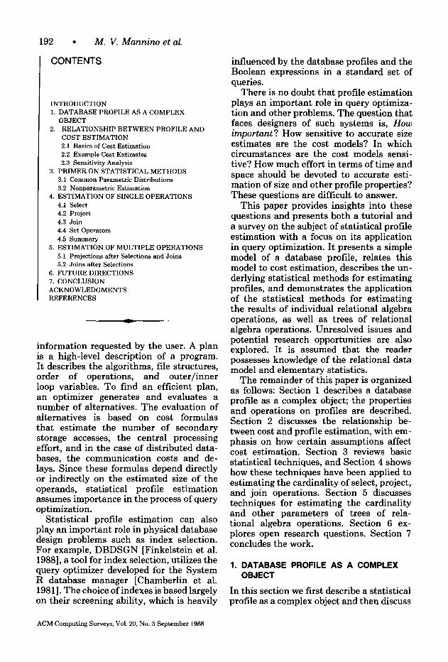
Cost estimates for these four strategies are derived under three scenarios: (1) actual sizes, (2) size estimates under assumptions of uniformity and independence, and (3) size estimates using a two-dimensional histogram. Table 1 displays the two- dimensional histogram. We assume the actual number of qualifying tuples is 380. The estimate using the histogram is 490, which assumes the cells of the histogram are uniformly distributed. The estimate using uniformity and independence assumptions is 3000.’

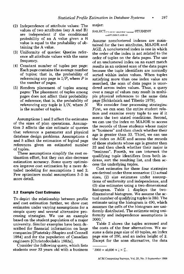
Table 2 shows the tuples accessed and the costs of the four alternatives. We assume a data page size of 40 tuples, an index page size of 250, and an index height of 2. Except for the scan alternative, the data

1 3000 = 40,000 x 1 x =. 8 45



Table 1. Two-Dimensional Histogram

AGE

MAJOR 16-20 21-25 26-30 31-35 36-40 41-60 Total

Business 2,045 3,600 3,625 Education 215 500 750 Engineering 750 1,800 1,775 Liberal arts 2,250 3,000 3,600 Public administration 250 575 875 Natural Science 715 1,850 2,000 Nursing 225 550 375 Social Science 575 900 1,200

Total 7,145 12,775 14,200

400 175 155 625 250 100 450 125 100 500 400 250 425 250 125 150 150 75 200 120 30 500 225 100

3,250 1,695 935

10,000 2,500 5,000

10,000 2,500 5,000 1,500 3,500

40,000

Table 2. Cost Estimates of Four Alternatives under Three Size Estimates

MAJOR + Scan MAJOR index AGE index AGE indices

Actual Sizes Tuple references Index references page Data references page Total references page

40,000 10,000 3,780 380 0 41 16 57

1,000 1,000 3,184 317 1,000 1,041 3,200 374

Assumption Estimates Tuple references Index references page Data references page Total references page

Histogram Estimates Tuple references Index references page Data references page Total page references

40,000 5,000 24,000 3,000 0 21 97 118

1,000 995 15,984 955 1,000 1,016 16,081 1,073

40,000 10,000 3,930 490 0 41 17 58

1,000 1,000 3,322 390 1,000 1,041 3,339 448

page references are largely based on the formula provided by Whang et al. [1983], which assumes random placement of tuples among pages. For the AGE index, we use the formula of Schkolnick and Tiberio [1979] because it results in an unordered scan across index values. Their formula assumes a buffer size of one page, which penalizes unordered scans. The data page references for the MAJOR + AGE indexes are based on an ordered scan because we assume that the tuple identifiers that result from intersecting indexes are sorted.

In this example, the query optimizer would have made a poor choice if it relied on the uniformity and independence assumptions. The sequential scan rather than the use of both indexes would have been chosen, resulting in perhaps three times as many page accesses as needed. If the opti-


mizer did not consider the fourth strategy, the size estimates would not have made a major difference since the estimated costs are all in favor of the scan strategy.

In this example, the sensitivity between cost and size estimates is straightforward because of the characteristics of the query and because it involved only a single operator query in a centralized database environment. The sensitivity issues become much more complex when evaluating trees of relational algebra operations and when considering distributed environments.

2.3 Sensitivity Analysis

A number of studies have examined the relationship between profile and cost estimation. Some have analytically studied the bias when using certain assumptions,

Statistical Profile Estimation in Database Systems 199

whereas others have experimentally tested sensitivity. We first examine the analytical studies and then the experimental ones.

Christodoulakis [ 1984b] analyzed the implications of the five assumptions stated in Section 2.1 on database performance evaluation. He considered the effects of these assumptions on the problems of estimating the (1) expected page accesses for a given N records, (2) expected number of page accesses for all queries on an attribute, (3) expected number of page accesses for mul- tiattribute queries, and (4) distinct number of attribute values after a selection operation. He proved that these assumptions lead to worst-case cost estimates. For example, he demonstrated that the uniformity and independence assumptions lead to a worst-case estimate for the distinct attribute values. He also argued persuasively that optimizers that use them will often choose worst-case access strategies such as sequential scanning and sorting. Direct access structures will often be ignored because the pessimistic cost estimates favor the simpler structures.

Montgomery et al. [1983] compared the size estimates of selection and join operations using uniformity assumptions when the data are heavily skewed. They compared models of size estimation using formulas based on uniformity assumptions against their own based on a skewed data distribution. They validated their formulas by comparing their estimates against simulated data. For the selection case, they found that uniformity assumptions tended to overestimate the result by 200-300%. For the join case, they found the opposite result.

Mackert and Lohman [1986a, 1986b] experimentally validated the local and distributed cost models used for single table, sorting, and two table joins in R*. Their tests confirmed the contribution of CPU costs to the total costs especially for sort operations. For index scans and sorts, size estimation is an important factor in both the I/O and CPU components of their cost formulas. Their experiments also revealed that the optimizer overstates the cost of the nested loop join algorithm when the inner table fits in main memory and there is an index on its join column. They suggested

that the nested loop cost is very sensitive to three parameters: join cardinality, the outer table’s cardinality, and the buffer uti- lization. In the case of distributed joins, the buffer sensitivity is less important because there is less contention for buffer space among the two joined tables. The join cardinality, however, assumes more importance because of its influence on the number of messages and bytes transmitted.

Kumar and Stonebraker [1987] investigated the effects of join selectivity on the selection of the optimal nesting order for four and five variable queries. They developed a simulated query processor that be- haves similarly to the System R optimizer [Selinger et al. 19791 in that it considers two join algorithms (nested loops and merge scan), performs only two-way joins, and considers using secondary indexes on the inner join table. They measured the sensitivity of a query with respect to changes in the joint selectivity by the ratio between the cost of the optimal plan and the plan of interest. The best plan under varying selectivities was either the one that minimizes the average cost ratio or the one that minimizes the maximum cost ratio. They measured the sensitivity of four and five variable queries under a variety of join selectivities using this sensitivity factor. They assumed known input relation sizes and independence among join clauses. Their results demonstrated that the optimal plan is insensitive to varying join selectivities if the optimal plan is chosen according to their criteria. They did not, however, investigate the sensitivity when the optimal plan is chosen in a traditional manner without consideration of varying join selectivities.

Vander Zander et al. [1986] studied the impact of correlation of attributes on the assumption of random placement of tuples to pages. They tested the query, “Retrieve all tuples from relation R where R.B = constant” when R is clustered according to another attribute (say A). High correlation between A and B causes skewness in the distribution of tuples to pages, which vio- lates the random-placement assumption. Using simulation, they found that the difference between the estimated logical page references under the random-placement



assumption and the actual was significant either univariate or multivariate distribu- beyond a correlation of .4. With a correlations. Multivariate distributions are usually tion of .6, the estimates overstated actuals more difficult to estimate than univariate by 70%. When correlation approached 1, distributions because of the increasingly the estimates overstated actuals by almost complex manner in which the variables 3000%. may interact as their number grows. This

multivariate comnlexitv can be consider-

3. PRIMER ON STATISTICAL METHODS

In this section we discuss the statistical methods that are used in the remaining sections. Some acquaintance with basic statistical concepts is assumed.

In statistics, the population (relation) is the set of all observations (tuples) of interest. Each observation consists of one or more values of variables (attributes). An extremely important objective of statistical inference is to estimate the distribution of the population. Knowledge of the distribution conveys the ability to calculate which values of variables are most likely to occur, how many values should occur in specified ranges, summary measures such as mean and standard deviation, and so on.

Methods for estimating the distribution of a population can be divided into two basic types according to how much is known about the shape of the distribution. Parametric methods assume that the distribution has a form that is completely known except for a few parameters; the goal then becomes the estimation of those few remaining parameters. For instance, a population may be thought to have a normal distribution. This completely specifies the distribution except for its mean and standard deviation, which are then estimated. Nonparametric methods are the second type. These methods assume little or noth- ing about the form of the distribution, so the estimation task is often more difficult than with parametric methods. The histogram, or bar chart, is a simple, common nonparametric estimate.

Methods for estimating the distribution of a population can also be divided into two basic types according to the number of variables measured per observation. Univariate populations have only one variable; multivariate populations have more than one variable. Both parametric and nonparametric methods may be used to estimate

ably simplified if the variables are statistically independent. If independence holds, then the multivariate distribution reduces to the product of the individual, or marginal, distributions of each variable. Independence can be tested by any of a collection of standard statistical tests such as the chi-square test for categorical variables or the correlation coefficient for continuous variables. Such tests, however, may be used only to reject the null hypothesis of independence-not to accept it.

Variables may also be classified according to the nature of their values into categorical and numerical types. To estimate the distribution of a categorical variable is to estimate the probability of occurrence of each category; summary measures such as the mean or standard deviation are either not calculable or inappropriate. The most general probability model for categorical variables is the multinomial. Numerical variables are either ratio scale (with a meaningful zero point) or interval scale (with an arbitrary zero point). This is further complicated by the classification of numerical variables into discrete and continuous types. Discrete variables are distinguished from continuous ones in that discrete variables have repetitions or duplicates of the same values with positive probability, whereas the probability of duplicate values of continuous variables is zero. Discrete distributions are estimated parametrically by positing a model such as the binomial, multinomial, or Poisson, estimating the appropriate parameters, and then testing the goodness of fit, for example, by the chi-square test; they are estimated nonparametri- tally by tallying the occurrences of each different value, that is, a histogram. Most of the effort in modern statistics has been lavished on the more difficult task of estimating continuous distributions.



3.1 Common Parametric Distributions

The distributions that have been reported in the literature as models for profile estimation include the uniform, normal, Pearson family, and Zipf. The uniform is the simplest and may apply to all types of variables, from categorical to numerical and from discrete to continuous. For categorical or discrete variables, the uniform distribution posits equal probability for all distinct categories or values. In the case of a continuous variable, the uniform distribution has constant probability density over the range of possible values. In the absence of any knowledge of the probability distribution of a variable, the uniform distribution is a conservative, minimax assumption.

The normal distribution is a symmetric, unimodal, “bell-shaped” distribution for continuous variables. It has two parameters to estimate, the mean and standard deviation, which control the location and dispersion, respectively, of the variable. Many variables follow approximate normal distributions, particularly those obtained as the result of summing or averaging other pro- cesses. The normal distribution is the minimum entropy choice when the mean and standard deviation parameters are known.

Karl Pearson proposed the eponymous family that would provide a wide range of choice of shapes but also be sufficiently concise so that a few parameters would suffice. The Pearson family includes the normal, uniform, beta, F, t, and gamma, all of which arise as solutions to a single dif- ferential equation [Johnson and Kotz 19701,

1 dy b+x --= Y dx a0 + alx + a2x2’

for various choices of the constants. These four constants are related directly to the first four moments of the distribution and therefore provide an easy means for estimation of the distribution.

Zipf’s law for continuous variables has a density function proportional to a power of the abscissa and therefore provides a model for positively skewed variables with higher probability of outliers than the normal,

gamma, and others. The exponent of the abscissa is the only parameter to estimate. Attempts to find a generally applicable law of nature in Zipf’s law have met with mixed success.

3.2 Nonparametric Estimation

In order to avoid the restrictions of particular parametric methods, many researchers have proposed nonparametric methods for estimating a distribution. The oldest and most common of these methods is the histogram. The essence of the histogram is to divide the range of values of a variable into intervals, or “buckets” and, by exhaustive scanning or sampling, tabulate frequency counts of the number of observations fall- ing into each bucket. The frequency counts and the bucket boundaries are stored as a distribution table. The distribution table can be used to obtain upper and lower selectivity estimates. Within those bounds, a more precise estimate is then computed by interpolation or other simple techniques. As noted below, modern methods of density estimation have refined and extended the classical histogram.

There are several different types of histograms, or distribution tables, depending primarily on the criteria chosen to set bucket boundaries. In the equal-width table the widths of the buckets are equal, but the frequencies or heights are variable. In an equal-height table the widths are determined so that the frequency within each bucket is the same. In a variable-width table the widths are determined so that the frequency within each bucket meets some other criterion, such as the values being uniformly distributed.

The equal-width table corresponds to the classical histogram and is very easy to apply in selectivity estimates: Simply search the table for the first bucket that contains the constant of the relational expression and interpolate between the endpoints of the bucket. But there are several drawbacks to the equal-width method:

(1) Since the maximum error rate is determined by the height of the tallest bucket, some prior knowledge about the



(2)

distribution of attribute values is necessary to predict estimation accuracy.

The statistics literature offers little help in choosing bucket boundaries without some knowledge of the distribution. This lends that choice an arbitrary component, which can have a significant effect on whatever error measure is used.

The statistics literature offers more help in choosing the number of buckets. Ob- viously, the number of buckets should be increased with the number of records. Be- fore modern mathematical analysis of density estimation, Sturges’ rule [1926], based on the binomial distribution, offered an empirically satisfactory choice. The number of buckets for n records is 1 + logzn under this rule. But modern analysis has provided optimal rules for given data-set sizes and error measures [Tapia and Thompson 19781. Interestingly, Sturges’ rule agrees reasonably well with the modern rules for data sets up to 500 records. In addition to maximum error rate, the literature has studied the mean error rate and mean-squared error rate (corresponding to the principle of least squares), among others. With maximum, mean, or mean- squared error rate, the size of the error can be determined to within a multiple of a power of the data-set size without other knowledge of the distribution. But whatever error measure is used, even with optimal choices, the equal-width method is asymptotically inferior to more modern methods such as the kernel or nearest neighbor techniques. For example, with mean-squared error, the asymptotic rate for the equal-width method is O(n-2’3), whereas the modern methods are O(n-4’5) or better, where n is the number of records [Tapia and Thompson 19781.

Better error control can be achieved by varying the width. In the equal-height method, a relationship is established between the number of buckets and the maximum error rate. If all buckets have about the same height, the error rate can be easily controlled by increasing the number of buckets. In the field of density estimation, this is called the nearest neighbor tech-

nique. The difficult part is to establish bucket ranges that satisfy the equal-height criterion since some knowledge of the distribution is essential. In density estimation, establishing the bucket range would be done by ordering the attribute values and choosing bucket boundaries at every kth value. Since this might be expensive, an approximation based on training sets or sampling might be implemented. Moreover, the performance of this estimator is asymptotically improved by permitting overlapping buckets; that is, for each attribute value of potential interest, record the location of the bucket of its k nearest neighbors. As with the equal-width technique, analysis has established asymptotically optimal choices (up to order of n) for the number of buckets (and hence k) without requiring further knowledge of the distribution. Of course, as noted previously, the location of those buckets will depend on some distribution knowledge.

Knowledge of the large-n properties of this technique was significantly advanced by Moore and Yackel [1977], who showed the duality of several modern density estimation techniques including the nearest neighbor; that is, after proper adjustment for the differences between techniques, a large-n theorem proved for one technique could be translated into a similar theorem for another technique without further proof. For example, with optimal choices, the asymptotic mean-squared error of the nearest neighbor estimator is 0 ( ne4”‘) or better, and one should choose k about O(n4’5) with about O(n115) buckets. Fur- ther discussion about density estimation techniques is given by Wegman [1983] and Wertz 119781.

In the third type of distribution table, the width of each bucket is varied according to criteria other than equal frequency. In density estimation, this technique is called the variable kernel. The variable kernel technique is difficult to analyze, and few results about the error control and the number of buckets have been reported. General references describing the variable kernel are Wegman [1983] and Wertz [ 19781. Specific results are described by Devroye [1985] and Breiman et al. [1977].



The density estimation literature provides multivariate analogs of the equal- width and equal-height methods. In the equal-width case a grid of cells of equal area or volume can be laid down in the joint space of the attributes, and the number of tuples with combined values in each cell can be counted. In the equal-height case variably sized buckets, each containing approximately k nearest neighbors, can be determined. The new problem in the multivariate case is that the shape of the bucket must also be chosen. With the equal-width analog, squares (or cubes or hypercubes depending on the dimension) are a natural choice. If the range or variation of one attribute’s values is much less than another’s, however, a rectangle with its short side parallel to the axis of the low-variance attribute would be better. With the equal- height analog and overlapping buckets per- mitted, use Euclidean circles, spheres, or hyperspheres. A better choice, particularly for distributions thought to be close to multinormal, is Mahalanobis distance [Mahalanobis 19361, which yields ellip- ses. Defining distance as the maximum of marginal attribute distances yields squares. In most cases there are no clear guidelines for choosing a distance measure. If the buckets should be nonover- lapping, tolerance regions may be con- structed by the method of Fraser [1957, chap. 41. This method provides no gui- dance on choice of shapes but permits a wide mixture of varieties, all of which are shown to be statistically equivalent.

Each multivariate technique shares the same general advantages and disadvantages as its univariate counterpart. But much less is specifically known about any technique, and the error properties of each deteriorate as the number of attributes increases, even under optimal conditions. For example, the mean-squared error of the kernel density estimator is known to be O(n-4’(d+4)) [Cacoullos 19661, where n is again the number of records and d the number of attributes.

4. ESTIMATION OF SINGLE OPERATIONS

This section discusses estimation of the cardinality of the operators select, project,

join, union, difference, and intersection. The first three operators are the most important and are widely studied. Union is an important operator in distributed databases with horizontally partitioned relations, but otherwise it is not widely used in queries. Intersection and difference are used less frequently and are the least studied.

Our discussion makes frequent reference to the statistical methods described in Sec- tion 3. We note where database researchers have used standard parametric and nonparametric methods and where extensions and new methods have been developed. We also describe a third class of methods called ad hoc. These methods are based on integrity constraints or other knowledge of the database semantics and can be used to bound an estimate or compute a number.

4.1 Select

The output tuple cardinality of a select operation is estimated by the following formula:

OUTCARD = INCARD * SEL-(BOOLEXPR),

where INCARD is the input cardinality, BOOLEXPR is the_ associated Boolean expression, and SEL (X) is the selectivity estimation function that estimates the fraction of records satisfying its Boolean expression argument. The selectivity estimation method depends on the type of Boo- lean expression (Figure 4). We begin our discussion with methods for simple relational expressions, which are the founda- tion for the more complex conjunctive and disjunctive expressions.

4.1.1 Simple Relational Expressions

A simple relational expression is of the form (attribute) (comparison operator) (value), where (comparison operator) yields a true or false value. Traditional comparison operators are <, =, >, and so on. In an environment with abstract data types [Stonebraker et al. 19831, other comparison operators such as intersect and overlap are possible. The following query



Select-Project Boolean

Figure 4. Classification of Boolean expression terms.

contains a simple relational expression:

SELECT,,,,,,, AGE-25 (STUDENT).

Cardinality estimation of simple relational expressions depends on the operator and the estimation method. Of the traditional operators, estimation of expressions with only = and < are necessary. Estima- tion of expressions with other traditional operators such as > can be rewritten in terms of < and =. For example, the estimate of the cardinality of AGE > 35 can be written as

INCARD-(OUTCARD(AGE = 35)

+ OUTCARD(AGE < 35)),

where OUTCARD is the estimate of the number of tuples satisfying expression X.

Methods from all three types (ad hoc, parametric, and nonparametric) have been proposed to estimate the selectivity of simple relational expressions. Common ad-hoc methods are based on constraints about candidate keys and value bounds. If a query contains an equality expression on candidate key, the selectivity estimate is l/INCARD because at most one record can qualify. The value bound constraints are especially important for queries against views. Suppose a view contains students with a grade point average greater


than 3.5. If a query asks for students in the view with an average less than 3.5, the selectivity estimate is zero.

The use of integrity constraints is related to the antisampling work of Rowe [1985]. In this approach, certain statistics, such as mean, standard deviation, and mode, are computed on a larger population. These facts are then used to infer simple statistics on subset populations. Rowe demonstrated the use of this technique to compute count, mean, maximum, minimum, median, and mode. Antisampling, however, has never been directly applied to selectivity estimation.

For most cases, the selectivity cannot be estimated by inferences from integrity constraints. Some knowledge of the frequency distribution of an attribute is necessary. This knowledge can be obtained by using simple assumptions or a more detailed modeling with a parametric or nonparametric method. Early query optimizers such as System R [Selinger et al. 19791 relied on the uniformity and independence assumptions. This was primarily due to the small computational overhead and the ease of obtaining the parameters (maximum and minimum values).

The use of the uniform distribution assumption has been criticized, however, because many attributes have few occurrences


with extreme values. For example, few companies have very large sales, and few em- ployees are very old or very young. The Zipf distribution [Zipf 19491 has been suggested by Fedorowicz [1984, 19871 and Samson and Bendell [1983] for attributes with a skewed distribution such as the occurrence of words in a text.

Christodoulakis [1983a] demonstrated that many attributes have unimodal distributions that can be approximated by a family of distributions. He proposed a model based on a family of probability density functions, which includes the Pearson types 2 and 7 and the normal distributions. The parameters of the models (mean, standard variation, and other moments) can be estimated in one pass and can be dynamically updated. Christodoulakis demonstrated the superiority of this model over the uniform distribution approach using a set of queries against a population of Canadian engineers.

Nonparametric methods have been widely used over parametric ones because of limitations cited in Section 3. Database developers have used the three types of distribution tables described in Section 3: equal width, equal height, and variable width. To demonstrate these three types, we use the frequency distribution of the AGE attribute on 100 students (Table 3). Figure 5a displays a bar graph for an equal- width distribution table that is divided into four intervals of width five.

Because of the limitations of equal-width tables (see Section 3), database developers have proposed the other types. Piatetsky- Shapiro and Connell [1984] proposed an equal-height method for selectivity estimation. To achieve equal-height buckets, the BUILD operator sorts the underlying data values. Bucket or step values are determined by positions in the sorted list according to the following formula:

POS(i) = ROUND(l + i * N, 0)

N = (INCARD-1)

S

S = number of buckets

ROUND(i, j) rounds i to j digits to the right of the decimal place.

Table 3. Age Distribution

Age Number Cumulative

20 2 2 21 3 5 22 5 10 23 8 18 24 2 20 25 0 20 26 0 20 27 0 20 28 30 50 29 2 52 30 8 60 31 5 65 32 5 70 33 0 70 34 10 80 35 14 94 36 2 96 37 1 97 38 1 98 39 1 99 40 1 100

The steps are numbered 0 through S. Step 0 is always the first value in the sorted list, and step S is always the last position (IN- CARD). As an example, Figure 5b illustrates a bar graph of an equal-height distribution table for the AGE attribute with S equal to 4. The positions in the sorted list of AGE values for the buckets are 0,26, 51,76, and 100, respectively. Because of the sorting requirement, equal-height tables cannot be dynamically updated.

Intervals in equal-height tables are closed on both ends. In other words, step i includes all values u, where VAL(i - 1) 5 u I VAL(i). The fraction of records in step i is computed as follows: (POW) - POS(L’ - 1))

INCARD when i > o

FRAC(i) ={

when i = 0,

The method to obtain selectivity estimates is more complex for equal-height tables because the matching between a constant and a step value has more cases. Piatetsky-Shapiro and Connell [1984] describe eight cases, including the constant between step values and the constant matching one interior step value. Both the



Frequency

20-24 25-29 30-34 35-40

AGE

(a)

Frequency

40

30 25 25 25 25

(b)

Frequency

20-24 25-27 26 29-32 33 34-35 36-40 PGE

Cc)

Figure 5. Example distribution tables. (a) Equal width. (b) Equal height. (c) Variable width.

upper and lower bounds and the within- bounds methods depend on these cases. Once a case is determined, the calculation is straightforward.

Muralikrishna and Dewitt [1988] extended the equal-height method for multidimensional attributes such as those based on point sets. Multidimensional attributes are very common in geographical, image, and design databases. A typical query with a multidimensional attribute is to find all the objects that overlap a given grid area. The authors proposed an algorithm to construct an equal-height histogram for multidimensional attributes, a storage structure, and two estimation techniques.

Their estimation techniques are simpler than the single-dimension version because they assume that multidimensional attributes will not have duplicates. Performance analysis by the authors was conducted to compare the estimation techniques and the use of random sampling to construct the histogram.

Database researchers have also proposed variable-width distribution tables. Merrett and Otoo [ 19791, Kooi [ 19801, and Muthu- swamy and Kerschberg [1985] suggested that widths be set so that the values within each bucket are approximately uniformly distributed. Figure 5c illustrates a bar graph for a variable-width table for the AGE



Table 4. Nonsimple Relational Expression Types

Name Pattern

Parameteric (attribute) (camp-op)(parameter) Dyadic (attribute) (camp-op) (attribute) Functional {(attribute) 1 (func-expr)}(comp-op)(func-expr)

attribute where the buckets have been set according to the uniformity criterion. The storage overhead of the variable-width table can be more than the equal-width table because both the height and range of each bucket must be stored. None of these researchers provide a method to determine bucket ranges for a given maximum error rate. The database administrator is assumed to possess enough knowledge to as- sign appropriate bucket ranges.

Christodoulakis [ 19811 proposed a variable-width table based on a uniformity measure (the maximal difference criterion) for choosing bucket ranges. This criterion clusters attribute values that have a similar proportion of tuples; that is, the difference between the maximum and minimum pro- portions of the attribute values in the bucket must be less than some constant, which can depend on the attribute. This criterion minimizes the estimation error on certain values rather than the average error on all values. It seems most appropriate where queries are not uniformly spread over all attribute values.

Kamel and King [1985] proposed a method based on pattern recognition to construct the cells of variable-width distribution tables. In pattern recognition a frequent problem is to compress the storage for an image without distorting its appearance. In selectivity estimation the problem can be restated to partition the data space into nonuniform cells that minimize the expected estimation error subject to an upper bound on storage size. They begin by dividing the data space into equal-sized cells and computing a homogeneity measure for each cell. The homogeneity is the measure of the nonuniformity or dispersion around the average number occurrences per value in the cell. The homogeneity can be computed by the function defined by the authors or by sampling. Adjacent cells with similar homogeneity measures are folded

together by considering the physical prox- imity of cells and the resulting homogeneity of the new combined cell. The authors report experimental results of their homogeneity function but no more complete implementation of their method.

4.1.2 Nonsimple Relational Expressions

Nonsimple relational expressions are divided into three types, as shown in Table 4 and Figure 4. Parametric expressions have a run-time parameter; dyadic expressions involve a comparison of two attributes from the same relation; functional expressions have operators such as addition, multipli- cation, and pattern matching.

Ad-hoc estimation methods are frequently used for nonsimple expression types. The justifications for the use of ad- hoc methods are (1) nonsimple expression types are not common and (2) no estimation technique can handle arbitrarily complex functional expressions. In the remainder of this section we concentrate on estimation techniques for the following types of nonsimple relational expressions: (1) equality parametric expressions (2) functional expressions containing string attributes and meta characters, and (3) equality dyadic expressions.

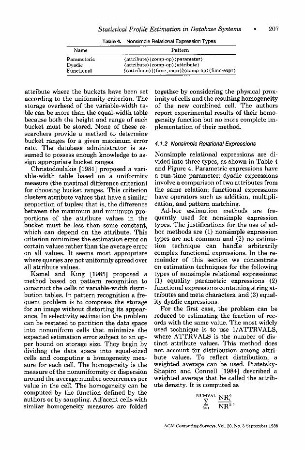
For the first case, the problem can be reduced to estimating the fraction of records with the same value. The most widely used technique is to use l/ATTRVALS, where ATTRVALS is the number of distinct attribute values. This method does not account for distribution among attribute values. To reflect distribution, a weighted average can be used. Piatetsky- Shapiro and Connell [1984] described a weighted average that he called the attribute density. It is computed as

NUMVAL x c is1 NR2’



where NRi is the number of record occurrences for value i, and i ranges over all distinct values. This gives extra weight to values associated with more than the average number of records.

Use of both the distinct values and the attribute density is based on no knowledge of the underlying parameter value. If a his- tory of values is maintained, a better estimate can be made. Christodoulakis [1983a] describes a method for estimating the average record selectivity over a collection of queries. His method estimates the average selectivity as a function of the standard deviation of attribute values in queries. This method has the advantage that it could be applied to parametric expressions with comparison operators other than equality.

The second case involves relational expressions with meta characters. A meta character does not match itself; instead, it matches a pattern of characters. Many query languages support meta characters to match (1) zero or more of any character, (2) any single character, and (3) any single character from an interval of characters. In Unify SQL [UNIFY 19851 these meta characters are *, ?, and [ 1, respectively. For example, the expression NAME = ‘A*’ matches names beginning with A.

The techniques for parametric queries cannot be applied since an arbitrary string with meta characters matches more than one value. Mannino [1986] describes a technique to translate an expression with meta characters into one or more expressions without meta characters. For example, the expression NAME = ‘A*’ can be translated into

NAME >= ‘A##### . . . #’

AND NAME <= ‘A@@@@@ . . . 0’

where # represents the low value in the attribute’s collating sequence and @ represents the high value. The estimation techniques for simple relational expressions can then be used. Mannino [ 19861 describes the translation of strings with a single wildcard character * or a single character class [ 1.

The third case involves equality dyadic expressions such as EMPLOYEE.SAL-

ARY = EMPLOYEE.COMMISSION. Lit- tle or no work has been reported on comparison operators other than equality. When the operator is equality, the methods described under join selectivity estimation (Section 4.3) can apply. In practice, methods assuming uniform distributions have been widely used. This is mostly due to the infrequent occurrence of simple dyadic expressions in select-project operations.

4.1.3 Boolean Combinations of Relational Expressions

Relational expressions can be combined with the Boolean operators AND and OR. In analyzing a Boolean expression, it is common to convert it into a standard form. A conjunctive normal form expression matches the pattern AND(X,, X2, . . . , X,,), where Xi is either a relational expression or a disjunction of relational expressions. In a disjunctive normal form expression, the position of the ANDs and ORs are swapped. Arbitrary Boolean expressions can be transformed into these normal forms through application of the laws of Boolean algebra such as the distribution of AND over OR and DeMorgan’s law. Jarke and Koch [1984] give a detailed explanation of the transformations.

To estimate the selectivities of conjunctive and disjunctive normal form expressions, one must be able to estimate the selectivities of conjunctive and disjunctive collections of relational expressions. Accu- rate estimation is difficult because the attributes in the relational expressions can be correlated. For example, the attributes sex, job title, and age group of many university faculties are often highly correlated. Correlation among attributes is difficult to account for because of the large number of attribute combinations.

The general formula for estimating the selectivity of a conjunctive expression is

SEL-(A and B)

= SEL-(A) * SEL-(B 1 A),

where A and B are relational expressions and SEL (B ] A) is the conditional probability of B given A [Clark and Schkade



19831. SEL (B ] A) indicates the degree of association between terms A-and B. If A and B are independent, SEL (B ] A) = SEL”(B) and the correlation can be ignored.

If the conjunctive expression involves a range such as in the following query, the formulas change:

SELECT FACUI,TY.SALARY<40.000 (FACULTY). ANDFAC”LTY.SALAHY>P”,OW

The possible cases for range queries are

(1) X 2 val-1 and X 5 val-2 (closed). (2) X > val-1 and X 5 val-2 (left open). (3) X L val-1 and X < val-2 (right open). (4) X > val-1 and X < val-2 (open).

The first case can be reformulated as a disjunctive expression:

1 - SEL-(X < val-1 OR X > val-2)

The other three cases can be similarly reformulated as disjunctive expressions.

The general formula for estimating the selectivity of disjunctive expressions is

SEL-(A OR B) = SEL-(A) + SEL-(B) .

- SEL (A and B).

This formula applies whether A and B are mutually exclusive or not. I,f A and B are mutually exclusive, the SEL (A AND B) is zero. Mutual exclusiveness is expected for terms related to the same attribute. For terms related to different attributes, the third term is evaluated as for conjunctive expressions.

Thus in both conjunctive and disjunctive expressions, if @tributes are not independent, the SEL (A AND B) must be estimated. Ad-hoc, parametric, and nonparametric methods can be used. As in the simple relational expression case, the most common ad-hoc method is based on candidate key constraints. The composite candidate rule can be used for conjunctive equality expressions containing a composite candidate key. Ad-hoc methods can also be based on value-combination rules. A value-combination rule states that attributes rarely assume values in certain combinations. Value-combination rules are

Table 5. Distribution Frequency on Age and Status

Age (X)

Status (Y)

Graduate Undergraduate

18-24 25-35 Over 35

150 400 50 800 150 20

generally not supported in most database systems.

For the parametric case, Christodoulakis [1983a] proposed a family of distributions defined by the multivariate normal distribution and the multivariate extensions of the Pearson type 2 and 7 distributions. As in the univariate case described earlier, these distribution families encompass a wide range of theoretical distributions and can be dynamically updated. In addition, any subset of attributes from a member of these distribution families conforms to the same distribution as the entire collection. This is important, since most queries will reference only a subset of the attributes.

Multivariate nonparametric methods are important because of the scale restriction of parametric methods, and it can be difficult to match the actual distribution of an attribute collection to a known theoretical one. The basic idea is to use a matrix in representing the relationship between attributes. In two dimensions, the row vector and the column vector represent the subdomains of the two attributes. Within cell X(i)Y(j) is the count of tuples whose value for attribute X falls in subdomain i and whose value for attribute Y falls in subdomain j. Table 5 shows how this approach can be used in estimating selectivity involving conjunctive or disjunctive query expressions.

If the query is about the number of students who are either of graduate status aged over 35 or of undergraduate status aged under 25, the answer is 850 (the count in cell X(3)Y(l) plus the count in cell X(l)Y(2)). If we alter the first term to the graduate students 35 or over, part of cell X(2)Y(l) qualifies. As in the case of univariate frequency distributions, an estimation error is possible because we do not know the distribution within a cell. As described in Section 3, less is known



about error control for multivariate distribution tables than for their univariate counterparts.

Multivariate nonparametric methods for selectivity estimation have been proposed by Merrett and Otoo [1979], Muthuswamy and Kerschberg [ 19851, Christodoulakis [1981], and Kamel and King [1985]. As in the univariate case, only the latter two presented a method to compute cell boundaries. Christodoulakis [1981] described a method that combines the independence assumption with maintaining more information on cells that have large deviations from independence. He demonstrated how this method can improve tuple estimation of Boolean expressions of two attributes. He did not, however, analyze this method for n-dimensional expressions.

King and Kamel [1985] demonstrated that the storage requirements can be very large for an n-dimensional distribution table that is divided into equal-sized cells. For example, for a relation of 12 attributes where each may assume any of 100 different values, a cell size of 50 still requires almost 1 megabyte of storage. They also derived error bounds for n-dimensional distribution tables and showed that it is possible for a selectivity estimate to err by half the relation size regardless of the result size of the query. As a response, they proposed a method to compute cell boundaries based on pattern recognition. Their technique is an extension to that described in Section 4.1.1.

4.2 Project

The project operator computes a vertical subset of a relation. Input is a relation and a list of attributes. Output is a relation with only the attribute list and duplicate tuples removed. In this section we consider a single projection operator as a leaf node in an access plan. Only a relatively small amount of work has been reported on this problem because projections are frequently not leaf nodes. The work on projections after other operations (selections and joins) is described in Section 5.1.

Merrett and Otoo [1979] described a nonparametric approach toward estimating the

distribution of a projection. They assumed that the input relation is described by an n-dimensional distribution table divided into equal-sized cells. Assuming uniformity within the cells, they demonstrated an iterative formula for computing the distribution of a projection of any subset of the n attributes. Since projections do not contain duplicates, the resulting cell counts cannot exceed the width of a cell.

Gelenbe and Gardy [1982] described a nonparametric approach toward estimating the size of a projection of n columns. Input is the size of the relation, which they assumed is known with certainty. They assumed that attributes are uniformly distributed and independent and that the projection is randomly generated with a uniform distribution. Using a probabilistic argument, they derived formulas to compute the number of projections with size k and the expected size over all possible randomly generated projections. They also addressed the problem of computing projection sizes given a collection of functional dependencies that hold on a relation. They reduced this problem to one of computing the conditional expected value given that the number of values of the determinant attribute(s) is equal to the number of tuples.

Other approaches are based on fast ways to estimate distinct values. Piatetsky- Shapiro [1985] estimated the number of distinct attribute values by means of sampling. The proposed method assumes uniform distribution of values. Applied to nonuniform distributions, the method gives a lower bound on the number of distinct values. Astrahan et al. [1985] developed three probabilistic methods based on hash functions. Each method requires only one pass of the relation, no sorting, and a small amount of memory and computation. Es- timation error rates are claimed within 10%.

4.3 Join

Join is a derived, binary operator. In terms of primitive operators, it is a Cartes- ian product followed by selection and sometimes by a projection. The selection



operation contains a dyadic Boolean expression with an attribute from each relation in each term. The following query demonstrates a join followed by a projection

Primitive Relational Algebra:

PROJECT (NAME, MAJOR C~ELECT,,,,,NT.~~N

=ENROLLMENT.SSN (STUDENT TIMES ENROLLMENT)))

Using a join operator:

PROJECT(NAME, MAJOR (STUDENT JOINSTUDENT.SSN

=ENROLLMENT SSN ENROLLMENT))

When the comparison operator in the join is equality, it is called an equijoin. A frequent type of equijoin is the natural join in which one of the join attributes is projected out. The natural join is the most widely studied and frequently used join. Only crude estimation techniques have been proposed for nonequijoins.

When the attributes of only one relation are required as in the previous example, the operation is called a semijoin. A semijoin is literally half of a join. Rl SEMI-JOIN R2 is the tuples of Rl that join with at least one tuple from R2. In a distributed environment, Rl is called the receive relation and R2 is called the send relation because the join values of R2 are sent to the site of Rl. The previous query can be rewritten as follows using a semijoin;

PROJECT (NAME, MAJOR (STUDENT SEMI-JOIN,,,,,mssiv

=ENROLLMENT.SSN ENROLLMENT))

The semijoin is an important operator in distributed access plans because it is sometimes cheaper to transmit join attribute values than an entire relation. Ceri and Pelagatti [ 19841 summarize approaches to distributed query optimization using semijoins.

The output cardinalities of the join and semijoin can be computed by the following

formulas:

OUTCARD(JOIN)

= SEL-(JOIN)*INNCARD,,*INNCARD,,

OUTCARD(SEMI-JOIN)

= SEL”(SEMI-JOIN)*INNCARD,,

In the first formula, SEL”(JOIN) represents the fraction of the Cartesian product that participate? in the join. In the second formula, SEL (SEMI-JOIN) represents the fraction of Rl that joins with at least one tuple of R2. It is assumed that Rl is the receive relation.

In general, accurate estimation of join and semijoin selectivities is more difficult than select or project. In the latter cases information about univariate and joint frequency distributions is sufficient; in the former case this information is not enough. Information about the distribution of tuples with matching join values is also necessary.

The estimation problem is even more acute because select and project operations are normally performed before the more expensive join operations. The frequency distributions of the join columns can change after select and project operations. Reliance on the original frequency distributions can lead to pessimistic estimates. Section 5 describes the problem of estimating the distribution of join attributes to reflect previous select and project operations. In the remainder of this section, we assume that the join attributes are independent of other attributes, and hence that the join attribute distributions do not change as a result of previous operations.

Join and semijoin selectivity estimation methods can be divided into the ad-hoc, parametric, and nonparametric categories. Ad-hoc methods can provide bounds and sometimes an exact number. By definition, the join cardinality is at most the product of its operand relations, and the semijoin cardinality is at most the cardinality of the receive relation. For join, a tighter upper .bound can be computed if one or both tables has a unique join attribute. These rules can



be stated as follows:

if the join attribute(s) of Rl are unique and the join attribute(s) of R2 are unique

then OUTCARD(JOIN) 5 MIN(INCARD(Rl),

INCARD(R2))

if the join attribute(s) of Rl are unique and the join attribute(s) of R2 are NOT candidate

keys then OUTCARD(JOIN) 5 INCARD(R2)

Determining whether a join attribute is unique depends on both the underlying integrity constraints and the join operation. A join attribute is unique if (1) it is a candidate key and (2) its underlying base table is preserved in a one-to-one manner in the join input. A relation is preserved if it is a base relation or if each tuple joins with at most one tuple of the other relation. The first requirement depends on the static properties of an attribute, but the second depends on the position of the join operation in an access plan. For example, assume we join three relations (Rl, R2, and R3) with the following Boolean expression: Rl.Al = R2.A2 and R2.A3 = R3.A3. R2.A3 is a candidate key, but the other columns are not. If the join between R2 and R3 is performed first, the join cardinality is lim- ited by the input cardinality of R3. If the join of Rl and R2 is performed first, the join of (Rl, R2) and R3 will not satisfy any of the unique rules because R2 is not preserved in the output of JOIN(R1, R2).

A lower bound can be determined if one join attribute is complete [Kooi 19801. An attribute is complete if every value in the attribute’s domain maps to at least one tuple in the attribute’s table; in other words, the active domain of the attribute equals the theoretical domain. The complete property usually only applies to base relations because all occurrences of selected attribute values are frequently removed by earlier operations.

If attribute Rl.Al is complete, each tuple of R2 must join with at least one tuple of Rl. Therefore, the join cardinality must be at least the cardinality of R2. If both the unqiue and complete rules hold, an exact estimate can be computed. For example, if Rl.Al is unique and complete, the JOIN

cardinality equals the cardinality of R2. The combination of these rules can also apply to semijoins. For example, if R2 SEMI-JOIN Rl and Rl’s join attribute is unique and complete, the cardinality equals R2.

Because these rules often do not provide precise estimates, the uniform distribution assumption has also been used. Kooi [ 19801 and Ceri and Pelagatti [1984] give the following formula, which assumes that both join attributes are uniformly distributed over the tuples of Rl and R2 and the values of Rl.Al also appear as values in R2.A2:

SEL-(Rl JOINmA,+..mR2)

1

= VAL(Rl.Al)

A variation of this formula was used in System R by Selinger et al. [1979]; they assume uniform distribution of values and at least one of the join attributes is complete. A similar formula has been proposed in Goodman et al. [1981] and Hevner and Yao [1979] for semijoin estimation if the uniform distribution and matching value assumptions hold:

SEL-(Rl SEMI-JOIN RI Al R2.42 _ R2

VAL(R2.A2)

= VAL(Rl.Al) ’

Parametric methods have not been proposed for join or semijoin estimation. For the join operator, there is no precedent in the statistics literature. For the semijoin operator, a probability density function can be used to estimate the semijoin distribution table described later in this section. No work has reported such an approach, possibly because it may be difficult to find an appropriate density function.

Two types of nonparametric methods have been proposed. The first type is based on a weighted average of matching join values and the independence between the join attributes and the other attributes. Kerschberg et al. [1982] provide the basic formula: CffI nlin2i, where nl and n2 are the number of tuples in Rl and R2, respectively, that have value Vi, the ith element



in the domain of values taken on by attribute A, and M is the number of distinct values that attribute A has.

If kl and k2 records are selected from each of the relations before the join, the expected size of the join is shown to be (klk2/nln2) CE1 nlin2i, [Christodoulakis 1983133. The expected number of tuples of Rl after a semijoin is (k/n) Cgl P2;n; [Christodoulakis 1983b], where P2i is the probability that the ith element in the domain of values of attribute A is nonzero in relation R2, and k is the number of records isolated from selections or semijoin on other domains. The semijoin is performed by sending distinct values of R2 in A to the site containing Rl.

The second type of nonparametric method is based on a table approximating the distribution of tuples with matching join values. Kooi [1980] proposed a method that uses variable-width distribution tables on the join columns. He assumed that values within a cell are uniformly distributed. If both join attributes are described by distribution tables with N cells with corresponding ranges, the join cardinality is computed as follows:

N C,,,,/ * INCARD,, * CAzj * INCARD, c

j=l EVAIJ - EVA~,j-~

Here, CAl,j is the fraction of Tl tuples within cell j of attribute Al, and EVAl,j is the ending value of cell j. If the cell ranges do not coincide, Kooi [1980] provides another formula, which is equivalent to a lin- ear interpolation of the overlapping parts of cell ranges.

Muthuswamy and Kerschberg [ 19851 used a new type of distribution table in their nonparametric method. To estimate the cardinality of a semijoin operation, they used a semijoin matrix. Recall that in a semijoin, the join column values of one table (the send table) are sent to the site containing the other relation (the receive relation). Each row of the matrix represents a value range of a join column. The join value component of a row is the number of tuples of the receive relation that join with the send relation. The join ratio component is the join value divided by the number of

Table 6. Semijoin Distribution Table

Range JOINVAL JOINRATIO

l-10 40 40/60 11-20 35 35176 21-36 25 25/64

Table 7. Restrictions on Expression Type Arguments

Operator Expression Restrictions

SELECT Simple None Parametric Equality only Functional Equality only Dyadic Equality only

JOIN Simple Equality only Boolean Simple equality terms only

tuples of the send relation within the row’s range.

Table 6 shows an example semijoin matrix for the expression Rl SEMI- JOINRM=R~.A~ R2. The cardinality of the semijoin is 100, which is computed by summing the JOINVAL column. The cardinality of the send relation is 200, which is computed by summing the denominators of the JOINRATIO column.

The cardinality of a semijoin is computed by using a distribution table on the send table’s join attribute and the JOINRATIO column of the semijoin matrix. The result is a new distribution table for the join column of the receive relation. The cardinality can be easily derived from the new distribution table.

4.4 Set Operators

Little work has been reported on the estimation of union and difference operations. This is due to their infrequent appearance in user queries. In horizontally partitioned relations, union operations are used to combine partitions either before or after other operations. In this case, the union operations are not part of the original query but instead are added by the query optimizer “under the covers.”



Table 8. Summary of Estimation Methods

Method

Operator Ad-hoc Parametric Nonparametric

Select (Relational)

Select (Boolean)

JOIN (Relational)

Candidate key rule, Value constraints

Candidate key rule

Unique rule, complete rule

Many proposed Equal width, equal height, variable width

Multivariate normal, Multivariate exten- Pearson type 2 and 7 sions, independence

assumptions, and univariate distribution tables

None . Weighted matching value parameters; semijoin distribution table

Ceri and Pelagatti [1984] give rules to bound the cardinality of union and difference operations but no more precise formulas. We present rules for completeness:

OUTCARD(R1 UNION R2)

5 INCARD(R1) + INCARD(R2)

MAX(0, INCARD(R1) - INCARD(R2))

5 OUTCARD(R1 MINUS R2)

5 INCARD(R1)

4.5 Summary

We summarize this section in two tables. Table 7 lists the restrictions that apply to expression arguments of the select and join operators. The restrictions denote where little work has been reported except for crude estimates. For example, little work has been reported on nonequality dyadic relational expressions in select operations. Table 8 summarizes the estimation methods for the select and join operators. For brevity, we have included only the major expression type arguments. As shown, the independence assumption has played a very significant role in join estimation and a smaller, yet significant, role in select estimation.

5. ESTIMATION OF MULTIPLE OPERATIONS

In the previous section we described methods to estimate the size of individual relational algebra operations. These methods


are necessary but insufficient because a query is typically a tree of relational algebra operations rather than an individual operation. To extend single operator methods, one can make simplifying assumptions, such as independence of attributes, or estimate conditional parameter values. We highlight the use of assumptions and conditional parameter values in several typical sequences of operations: a projection preceded by a selection or join, and a join preceded by a selection. From these cases we generalize to methods for estimating arbitrary trees of selections, projections, and joins.

5.1 Projections after Selections and Joins

Computing the size of projections after selections and joins is important for estimating semijoin operations that follow the projection. Semijoins are frequently used in distributed database systems. The join column of one table is projected and sent to the site of another table where the semijoin occurs. As in the single operator case, most proposed methods are nonparametric.

For projections after selections, there are two cases to consider. First, one needs to estimate the size of an attribute used in a Boolean formula of a selection operation. Here, the size is proportional to the number of tuples, except in the case of a simple equality selection, where it is equal to 1 [Ceri and Pelagatti 19841. Second, one needs to estimate the distinct values of an attribute not used in a selection operation.


This problem is related to the classic statistics problem [Kotz and Johnson 19771:

Given n balls to distribute over m urns, what is the expected number of urns occupied when k balls are deposited?

When applying this problem to distinct value estimation, the balls are tuples and the urns are distinct values. This problem has also been applied to estimating logical page references and other physical database problems. In the logical page case, balls are tuples and urns are disk pages.

The latter problem has been investigated by many database researchers over the last 15 years. Most work has been dominated by the following assumptions:

(1)

(2)

(3)

(4)

Records are selected without replacement. The variables n, m, and k are known constants. There is a constant number of tuples per page. There is random placement of tuples among pages.

Cardenas [ 19751 developed the following formula for the expected number of page accesses under the above assumptions, except that tuples are selected with replacement:

This formula can be derived by noting that l/m is the probability that a page contains a tuple, [ 1 - (l/m)] k is the probability that a page does not contain any of the k tuples, and 1 - [l - (l/m)] k is the probability that a page contains at least one of the k tuples.

The above formula has undergone revision by several researchers. Yao [1977] noted that the formula assumes sampling with replacement, which is unrealistic in the page access problem because a tuple can be selected at most once. He thus derived an exact formulation without replacement and demonstrated that when the blocking factor is 10 or more, the simpler without-replacement formula provides almost identical results. Cheung [1982] developed a new formula when the requested

tuples may have duplicates. He also developed a simple formula for estimating the number of distinct tuples referenced in a transaction. One of Yao’s equations requires iteration and can be expensive to compute if k is large. As a response, Whang et al. [1983] devised a closed, noniterative approximation. They demonstrated that their formula has a maximum error of 3.7% and that the computation time is significantly reduced by eliminating the iterative loop.

More recently, researchers have relaxed some of these assumptions. The assumption that k is a constant is unrealistic because it must be estimated in most cases. Luk [1983] proved that, if k is a random variable instead of a constant, Yao’s formula overstates the number of pages. He gave a general guideline to follow when Yao’s formula is used for varying k.

A number of researchers have replaced the assumptions of a constant number of balls per urn and random placement with detailed modeling. The basic idea is to represent the page access frequency as a vector p = ( pl, . . . , p,), where pi is the probability of accessing page i. With the random-placement assumption each probability is l/m. Christodoulakis [1984a] modeled the distribution of records to pages by attribute values using multivariate distributions based on the Pearson and normal families. By integrating the distribution over the appropriate attribute values, he derived a page access distribution for a particular query. This derived distribution was then used to compute the expected number of page accesses.

Vander Zander et al. [ 19861 examined the problem of estimating the number of logical page accesses given a selection query with one simple, equality relational expression on an attribute (say A) but where the relation is clustered according to another attribute (say B). If A and B are highly correlated, the distribution of tuples to pages for the query is highly skewed and the random placement assumption may lead to poor estimates. To account for possible skewness resulting from correlations, they proposed a nonparametric method to model page distributions and two ways to build a discretized or compacted



distribution. The first method partitions a distribution such that pages with access frequency greater than the mean are grouped together in one cell, with the remaining pages in another cell. The second method accounts for the number of selected records (k) through multiple page distributions: One for the overall distribution of tuples to pages and other distributions for the most frequently, the average, and the least frequently occurring value of each attribute. For a given query they chose an appropriate distribution based on the attribute and the expected size of the answer, dynamically modified it, and computed the expected number of pages. They compared both methods against actual page accesses using simulation. Their analysis provided guidelines for using the random-placement assumption and compacted page distributions of sizes 2 and 4.

Several others have also examined the implications of the random-placement assumption. Zahorjan et al. [1983] used a technique from queuing theory to construct a distribution vector for estimating the expected page accesses. Luk [1983] used the Zipf distribution as a model of a ball distribution. Ijbema and Blanken [ 19861 defined a class of ball distributions and derived tight upper and lower bounds for the estimation. They demonstrated that Yao’s formula gives results on the upper bound, whereas Luk’s gives results often beneath their lower bound. In addition, they proposed a computationally efficient approximation for the bounds.

For the problem of estimating the distinct values after a join or semijoin operation, the previous formulas have also been applied. Bernstein et al. [1981] gave an approximation formula for semijoin estimation in a distributed database system. Their formula, however, relied on the constant-size and random-placement assumptions. Christodoulakis [ 1983b] introduced an alternate formula:

VAL(0UT.A) = ; PljPZ;, ,=I

where M is the number of distinct values in the domain of A and Pl, and P2i are the probability that the ith element in the do-

main of values of attribute A is nonzero in relations Rl and R2, respectively. In this formula, only independence of attributes is assumed.

The distribution model of Merrett and Otoo [1979] can be applied to projection sizes after selections or joins because it estimates conditional distributions rather than just sizes. This and other approaches that work with conditional distributions are described in the following section.

In addition to deriving the expected number of distinct values mathematically, inference on bounds can be made using rules such as

if A is a join attribute then VAL(0UT.A)

5 MIN(VAL(Rl.A), VAL(R2.A))

if A is not a join attribute then VAL(0UT.A)

5 VAL(R1.A) + VAL(R2.A).

5.2 Joins after Selections

In the description of join estimation in Section 4.3, it was assumed that either the join was performed on a base relation or that independence holds among the attributes. Since the independence assumption is suspect and joins are often not performed on base relations, more detailed modeling of the correlation can produce better estimates.

The concept of conditional probability has been applied to account for correlations among attributes in a tree of relational algebra operations. Conditional probability applies to multioperation access plans because the result of a previous operation may affect the statistical properties of attributes in a later operation. Consider two attributes X and Y that are described by a multivariate distribution. A selection outputs attribute Y and qualifies tuples by a Boolean expression involving attribute X. A later join operation uses attribute Y in its Boolean expression. To estimate the join cardinality, one must first estimate the marginal conditional distribution of Y given the Boolean expression on X. The attributes with the conditional distribution to estimate are called indirect because they do not participate in the Boolean



EST-CARD(STUDENT SEMIJOIN ENROLLMENT)

I EST-DlST(ENROLLMENT.SSN)

I EST-CARD(ENROLLMENT SEMIJOIN OFFERING)

I EST-DIST(ENROLLMENT.UNlQUENO)

EST-CARD(GRADE >= 90)

EST-DlST(OFFERlNG.UiWWENO)

EST-CARD(SEMS=‘SPRING’ AND YEARd36)

Figure 6. Profile estimation operations.

expression of the previous operation. The attributes in the Boolean expression of the previous operation are called direct.

Figure 6 shows the profile estimation operations for the following relational algebra expression:

STUDENT SEMI-JOIN~T~~~~~.~~~ =ENHOLLMENT.SSN

(SELECT ENROLLMENTGRADE>SO (ENROLLMENT) SEMI-JOIN ENROI.LMENT.*NIQ”ENO

=OFFERING.“NIQ”ENO

In the expression, OFFERING and EN- ROLLMENT are combined first, followed by STUDENT. In the profile estimation operations, the conditional distributions of the join attributes (OFFERING.UNIQUE- NO, ENROLLMENT.UNIQUENO, AND ENROLLMENT.SSN) are estimated to reflect the previous operations. STU- DENT.SSN is not estimated because no select operations are performed on STU- DENT.

If a parametric method is used to compute joint probabilities, the conditional marginal distribution can be computed by applying the probability density function. For example, if attributes X and Y are described by a bivariate normal distribution, the conditional marginal distribution of Y after the selection X > 10 can be

computed by dividing normal bivariate density by the integral from 3c = 10 to infinity.

If a nonparametric approach is used, the approaches described by Merrett and Otoo [1979] and Muthuswamy and Kerschberg [1985] can be used. In both approaches the result of an estimation operation is a derived distribution of the resulting relation. For direct attributes, the derived distribution is computed by excluding the cells outside of the Boolean expression. For indirect attributes Muthuswamy and Kersch- berg combine the multivariate distribution table with the marginal distribution on the direct attribute to produce the conditional marginal distribution of the indirect attribute. In matrix algebra, their formula is Ai = Ad X Mdi, where Ad is the marginal frequency of the direct attribute after the selection, Ai is the conditional marginal frequency of the indirect attribute, and Mdi is the matrix representing the joint frequency divided by the product of the marginal frequencies of the direct and indirect attribute. Merrett and Otoo [1979] also covered the case in which the indirect attribute is projected (i.e., duplicates are removed). This case is important in distributed database systems where projections are sometimes transmitted from one site to another.



We can generalize from this discussion of conditional probability to two ways of estimating arbitrary sequences of selections, projections, and joins. In the stand- alone approach, the methods for each operator are independent. The only information available to a method is the base profiles and the estimated sizes of intermediate results. This simplifies the estimation process because only the output size is computed. It also means that estimation methods need not be compatible because they only share the computed size. The estimation accuracy suffers, however, because conditional parameter values are not used. In the integrated approach, the methods for operators must be compatible because they use conditional profile values as well as output sizes. The time and space requirements for computing and saving the conditional values may add considerable overhead to the estimation process, but better estimates are possible.

6. FUTURE DIRECTIONS

Open research issues can be classified as (1) use of other decision-theoretic concepts, (2) statistical modeling of logical and physical page references, and (3) extensi- bility. Decision theory influences selectivity estimation in two ways. First, in the estimation of tuple cardinality in Sec- tion 4, most attention was devoted to estimating the maximum error rate. This is a strategy of minimizing the maximum error, which implies the use of equal-height rather than equal-width methods. That strategy may be unduly conservative. In decision- theoretic terms it is a minimax strategy. Future work might look into the applica- bility of other criteria such as mean- squared error. Second, in order to reflect one’s knowledge of the distribution of an attribute’s values, the use of prior distributions is useful. Prior distributions can be updated to posterior distributions by following a Bayes strategy: Take a small sample and use an appropriate loss function (e.g., maximum error, mean error, or mean- squared error) to minimize risk. To a degree, parts of this regimen have already been proposed in rudimentary form. For

example, the presumption of attribute value distribution being some specified parametric form such as normal, the parameters of which are periodically updated, is a partial and unconscious implementation of the empirical Bayes approach. A conscious implementation has much to recommend it: exploitation of the database administrator’s knowledge of the attribute; ease in updating statistical profiles, flexibility to future changes, risk minimization, and a developed body of applicable knowledge in the statistical literature.

The second research direction deals with detailed statistical models for estimating the logical and physical page references. Some unrealistic assumptions are often made in estimating logical page references, but recent work such as Vander Zander et al. [1986] provides an excellent start to replace the simplifying assumptions with detailed modeling. The effects of buffer space are rarely accounted for in estimating physical page references. Recently, some researchers have proposed models that fea- ture more detailed modeling in place of the simplifying assumptions. Copeland et al. [1986] used statistics to model the changing locality of reference to database pages. Mackert and Lohman [1985] developed a model for index scans, which relaxes the assumption of unlimited buffer space. These papers represent an important step in more accurately modeling the effect of buffer space on a plan’s resource usage.

The third research direction is extensi- bility. An extensible database system [Batory and Mannino 19861 can be easily configured to meet the needs of emerging application areas such as computer-aided design, multimedia systems, and statistical analysis. An extensible approach to profile estimation separates methods from the profile operators. When an operator is applied, it is responsible for selecting a method from a collection chosen by the database designer. This separation permits flexibility in the modeling of distributions, correlation, relational expression types, and access plan operators. An extensible model of tuple cardinality estimation for selections has been proposed by Mannino and Rivera [1988].



7. CONCLUSION

A statistical profile summarizes the instances of a database. It typically describes the number of instances, the distribution of values, the correlation between value sets, and the number of distinct values. Accurate estimation of profiles is important in query optimization and sometimes in physical database design and performance evaluation. A precise characterization of the value of accurate profiles, however, is still an open issue because of the large number of cases to consider and the need to measure the sensitivity on the choice of access plans.

We described three operators on profiles: The BUILD operator creates a profile from a base object either through an exhaustive scan or a sample; the UPDATE operator revises a base profile to reflect updates to its underlying base object; the ESTIMATE operator computes an intermediate profile using one or more profiles and an operation description.

The methods for the ESTIMATE operator were classified by the type of method (ad hoc, parametric, and nonparametric) and the relational algebra operator. Ad-hoc methods provide bounds and sometimes exact estimates. They typically are based on the existence of integrity constraints such as candidate keys. Parametric methods use a probability density function and a small collection of parameters that can be computed by arithmetic on attribute values. They require that the attributes have at least an interval scale. Nonparametric methods use parameters that can be computed on value counts. They can be more costly in terms of storage and computation time, but they do not suffer from goodness- of-fit and attribute scale limitations. We described the methods for individual relational algebra operations as well as for trees of operations.

ACKNOWLEDGMENTS

We thank Jeff Mischkinsky, Angel Rivera, Chou Lin Chen, Kuo Tay Chen, and Betsy Greenberg for help- ful discussions. We also thank the referees and the editor for a very thorough review and many useful suggestions.

REFERENCES

APERS, P. M. G., HEVNER, A. R., AND YAO, S. B. 1983. Optimization algorithms for distributed queries. IEEE Trans. Softw. Eng. SE-g, 1, 57-68.

ASTRAHAN, M., SCHKOLNICK, M., AND WHANG, K. 1985. Counting unique values of an attribute without sorting. Tech. Rep. RJ 4960, IBM Re- search Division.

BATORY, D., AND MANNINO, M. 1986. Panel on extensible database systems. In Proceedings of the ACM SZGMOD Conference (Washington, D.C., May). ACM, New York, pp. 187-190.

BERNSTEIN, P., GOODMAN, N., WONG, E., REEVE, C., AND ROTHNIE, J. 1981. Query processing in SDD-1: A system for distributed databases. ACM Trans. Database Syst. 6, 4 (Dec.), 602-625.

BREIMAN, L., MEISEL, W., AND PURCELL, E. 1977. Variable kernel estimates of multivariate densi- ties. Technometrics 19, 135-144.

CACOULLOS, T., 1966. Estimation of a multivariate density. Ann. Inst. Stat. Math. 18, 178-189.

CARDENAS, A. 1975. Analysis and performance of inverted data-base structures. Commun. ACM 18, 5 (May), 253-263.

CERI, S., AND PELAGATTI, G. 1984. Distributed Databases: Principles & Systems. McGraw-Hill, New York.

CHAMBERLIN, D., ASTRAHAN, M., KING, W., LORIE, R., MEHL. J.. PRICE, T., SCHKOLNICK, M.. GRIFFITHS’SE~INGER, P., KLUTZ, D., WADE, B.; AND YOST, R. 1981. Support for repetitive transactions and ad hoc queries in system R. ACM Trans. Database Syst. 6, 1 (Mar.), 70-94.

CHEUNG, T. 1982. Estimating block accesses and number of records in file management. Commun. ACM 25, 7 (July), 484-487.

CHRISTODOULAKIS, S. 1981. Estimating selectivities in data bases. Ph.D. dissertation, CSRG-136, Computer Systems Research Group, Univ. of Toronto.

CHRISTODOULAKIS, S. 1983a. Estimating record selectivities. Znf. Syst. 8, 2 105-115.

CHRISTODOULAKIS, S. 1983b. Estimating block transfers and join sizes. In Proceedings of the ACM SZGMOD Conference (May). ACM, New York, pp. 40-54.

CHRISTODOULAKIS, S. 1984a. Estimating block selectivities. Znf. Syst. 9, 1, 69-79.

CHRISTODOULAKIS, S. 1984b. Implications of certain assumptions in database performance evaluation. ACM Trans. Database Syst. 9, 2 (June), 163-186.

CLARK, C., AND SCHKADE, L. 1983. StatisticalAnaZy- sis for Administrative Decisions. South-Western, Cincinnati.

COPELAND, G., KHOSHAFIAN, S., SMITH, M., AND VALDURIEZ, P. 1986. Buffering schemes for per- manent data. In Proceedings of the Conference on Data Engineering (COMPDEC) (Los Angeles, Calif., Feb.). IEEE, New York, pp. 214-221.



DEVROYE, L. 1985. A note on the L, consistency of variable kernel estimates. Ann. Stat. 13, 1041-1049.

DEWITT, D., KATZ, R., OLKEN, F., SHAPIRO, L., STONEBRAKER, M., AND WOOD, D. 1984. Implementation techniques for main memory database systems. In Proceedings of the ACM SZG- MOD Conference (Boston, Mass. June). ACM, New York, pp. 1-8.

FEDOROWICZ, J. 1984. Database evaluation using multiple regression techniques. In Proceedings of the ACM SZGMOD Conference (Boston, Mass., June). ACM, New York, pp. 70-76.

FEDOROWICZ, J. 1987. Database performance evaluation in an indexed file environment. ACM Trans. Database Syst. 12, 1 (Mar.), 85-110.

FINKELSTEIN, S., SCHKOLNICK, M., AND TIBERIO, P. 1988. Physical database design for relational databases. ACM Trans. Database Syst. 13, 1 (Mar.), 91-128.

FRASER, D. 1957. Nonparametric Methods in Stutk- tics. Wiley, New York.

GELENBE, E., AND GARDY, D. 1982. The size of projections of relations satisfying a functional dependency. In Proceedings of the 8th Znterna- tional Conference on Very Large Data Bases (Mexico City). Very Large Data Base Endow- ment, Saratoga, Calif., pp. 325-333.

HEVNER, A., AND YAO, S. B. 1979. Query processing in distributed database systems. IEEE Trans. Softw. Eng. SE-3,3.

IJBEMA, A., AND BLANKEN, H. 1986. Estimating bucket accesses: A practical approach. In Pro- ceedings of the Conference on Data Engineering (COMPDEC) (Los Angeles, Calif., Feb.), pp. 30-37.

JARKE, M., AND KOCH, J. 1984. Query optimization in database systems. ACM Comput. Suru. 16, 2 (June), 111-152.

JOHNSON, N., AND KOTZ, S. 1970. Distributions in Statistics: Continuous Univariate Distributions, ~01s. 1 and 2. Houghton Mifflin, Boston.

KAMEL, N., AND KING, R. 1985. A model of data distribution based on texture analysis. In Pro- ceedings of the ACM SZGMOD Conference (Aus- tin, Tex., May). ACM, New York, pp. 319-325.

KERSCHBERG, L. TING, P. D., AND YAO, S. B. 1982. Query optimization in star computer net- works. ACM Trans. Database Syst. 7, 4 (Dec.), 678-711.

KOOI, R. 1980. The optimization of queries in relational databases. Ph.D. dissertation, Case West- ern Reserve Univ., Cleveland, Ohio.

KOTZ, S., AND JOHNSON, N. 1977. Urn Models and Their Application. Wiley, New York.

KUMAR, A., AND STONEBRAKER, M. 1987. The effect of join selectivities on optimal nesting order. SZGMOD Rec. 16, 1 (Mar.), 28-41.

LOHMAN, G., MOHAN, C., HAAS, L., LINDSAY, B., SELINGER, P., WILMS, P., AND DANIELS, D. 1985. Query processing in R*. In Query Process- ing in Database Systems, W. Kim, D. Batory, and

D. Reiner, Eds. Springer-Verlag, New York, pp. 31-47.

LUK, W. 1983. On estimating block accesses in database organizations. Commun. ACM 26, 11 (Nov.), 945-947.

MACKERT, L., AND LOHMAN, G. 1985. Index scans using a finite LRU buffer: A validated I/O model. IBM Research Ren. RJ4836. Almaden Research Center, San Jose, Calif.

MACKERT, L., AND LOHMAN, G. 1986a. R* optimizer validation and performance evaluation for local queries. In Proceedings of the ACM SZGMOD Conference (Washington, D.C., May). ACM, New York, pp. 84-95.

MACKERT, L., AND LOHMAN, G. 1986b. R* Optimizer validation and performance evaluation for distributed Queries. In Proceed&s of the 12th Znter- - national Conference on Very Large Databases (Kyoto, Japan, Aug.). Morgan Kaufmann Pub- lishers, Inc. (Also IBM Research Report RJ5050, Alamaden Research Center, San Jose, Calif.)

MAHALANOBIS, P. 1936. On the generalized distance in statistics. In Proceedings of the National Znsti- tute of Sciences of India 12, pp. 35-49.

MANNINO, M. 1986. Selectivity estimation in unify SQL. Tech. ROD. Dept. of Management Science and Information Systems, Univ. of Texas, Austin.

MANNINO, M., AND RIVERA, A. 1988. An extensible model of selectivity estimation. Znf. Sci.-An Zn- tern&ion& Journal. Special issue on database systems to appear Spring 1988.

MERRETT, T. H., AND 0~00, E. 1979. Distribution models of relations. In Proceediws of the 5th International Conference on Ve@ Large Data Bases (Rio de Janeiro, Brazil. Oct.). ACM, New York, pp. 418-425.

MONTGOMERY, A., D’SOUZA, D., AND LEE, S. 1983. The cost of relational algebraic operations on skewed data: Estimates and experiments. In Information Processing Letters 83. Elsevier North-Holland, New York, pp. 235-241.

MOORE, D., AND YACKEL, J. 1977. Consistencyprop- erties of nearest neighbor density function estimates. Ann. Stat. 5, 143-154.

MURALIKRISHNA, M., AND DEWIIT, D. 1988. Equi- depth histograms for estimating selectivity factors for multi-dimensional queries. In Proceed- ings of the ACM SZGMOD Conference (Chicago, Ill., June). ACM, New York, pp. 28-36.

MUTHUSWAMY, B., AND KERSCHBERG, G. 1985. A DDSM for relational query optimization. Tech. Rep., Univ. of South Carolina, Columbia. Also in Proceedings of the ACM Annual Conference (Denver, Colo., Oct.). ACM, New York.

PIATETSKY-SHAPIRO, G., AND CONNELL, G. 1984. Accurate estimationof the number of.tuples satisfying a condition. In Proceedings of the ACM SZGMOD Conference (Boston, Mass., June). ACM, New York, pp. 256-276.

PIATETSKY-SHAPIRO, G. 1985. Estimating the number of distinct attribute values by using sampling. Submitted for publication.



ROWE, N. 1985. Antisampling for estimation: An TEOREY, T. AND FRY, J. 1982. Design of Database overview. IEEE Trans. Softw. Eng. 11.10 (Oct.).. Structures. Prentice-Hall, Englewood, Cliffs, N.J. - , - 1081-1091. UNIFY CORPORATION. 1985. Unix Relational Data-

SAMSON, W., AND BENDELL, A. 1983. Rank order base Management System-Reference Manual. distributions and secondarv key indexing (ex- Release 3.2. Portland, Oreg. tended abstract). In Proceedings of the 2nd>nter- national Conference on Databases, (Cambridge, England).

SELINGER, P., ASTRAHAN, M., CHAMBERLIN, D., LORIE, R., AND PRICE, T. 1979. Access path selection in a relational database management system. In Proceedings of the ACM SZGMOD Conference (San Jose, Calif.). ACM, New York, pp. 23-34.

SCHKOLNICK, M., AND TIBERIO, P. 1979. Con- siderations in developing a design tool for a rela-

VANDER ZANDER, B., TAYLOR, H., AND BITON, D. 1986. Estimating block accesses when attributes are correlated. In Proceedings of the 12th Znter- national Conference on Very Large Databases (Kyoto, Japan, Aug.). Morgan Kaufmann Pub- lishers, Inc., pp. 119-127.

WEGMAN, E. 1983. Density estimation. In Encyclo- pedia of Statistical Sciences, Vol. 2, S. Kotz and N. Johnson, Eds. Wiley, New York.

WERTZ, W. 1978. Statistical Density Estimation: A Suruev. Vandenhoeck and Runrecht. Gottinzen.

tional DBMS. In Proceedings of the IEEE COMPSAC Conference (Chicago, Ill., Nov.).

WHANG, K., WIEDERHOLD, G., AND SAGALOWICZ, D.

IEEE Press, New York, pp. 228-235. 1983. Estimating block accesses in database oreanizations: A closed noniterative formula.

STONEBRAKER, M., RUBENSTEIN, B., AND GUTMANN, Cimmun. ACM 26, 11 (Nov.), 940-944. A. 1983. Application of abstract data types and abstract indices to CAD databases. In Proceed-

YAO, S. 1977. Approximating block accesses in da-

ings of Database Week: Engineering Design Ap- tabase organizations. Commun. ACM 20,4 (Apr.), 260-261.

plications (San Jose, Calif., May). pp. 107-113. ZAHORJAN, J., BELL. B., AND SEVCIK, K. 1983. STURGES, H. 1926. The choice of class interval. Estimating block transfers when record access

J. Am. Stat. Assoc. 65-66. probabilities are non-uniform. Znf. Process. Z&t. TAPIA, R., AND THOMPSON, J. 1978. Nonparametric 16, 5 (June), 249-252.

Probability Density Estimation. John Hopkins ZIPF, G. 1949. Human Behavior and the Principle of University Press, Baltimore, Md. Least Effort. Addison-Wesley, Cambridge, Mass.

Received March 1987; final revision accepted May 1988.


Documents

Statistical Profile Estimation in Database Systemspeople.csail.mit.edu/tdanford/6830papers/mannino-stat-profile-estimation.pdfStatistical Profile Estimation in Database Systems