1

Statistical Process Control

Prof. Robert C. Leachman IEOR 130, Methods of Manufacturing Improvement

Spring, 2014 1. Introduction Quality control is about controlling manufacturing or service operations such that the output of those operations conforms to specifications of acceptable quality. Statistical process control (SPC), also known as statistical quality control (SQC), dates back to the early 1930s and is primarily the invention of one man. The chief developer was Walter Shewhart, a scientist employed by Bell Telephone Laboratories. Control charts (discussed below) are sometimes termed Shewhart Control Charts in recognition of his contributions. W. Edwards Deming, the man credited with exporting statistical quality control methodology to the Japanese and popularizing it, was an assistant to Shewhart. Deming stressed in his teachings that understanding the statistical variation of manufacturing processes is a precursor to designing an effective quality control system. That is, one needs to quantitatively characterize process variation in order to know how to produce products that conform to specifications. Briefly, a control chart is a graphical method for detecting if the underlying distribution of variation of some measurable characteristic of the product seems to have undergone a shift. Such a shift likely reflects a subtle drift or change to the desired manufacturing process that needs to be corrected in order to maintain good quality output. As will be shown, control charts are very practical and easy to use, yet they are grounded in rigorous statistical theory. In short, they are a fine example of excellent industrial engineering. Despite their great value, their initial use in the late 1930s and early 1940s was mostly confined to Western Electric factories making telephony equipment. (Western Electric was a manufacturing subsidiary of AT&T. As noted above, the invention was made in AT&T’s research arm, Bell Laboratories.) Evidently, the notion of using formal statistics to manage manufacturing was too much to accept for many American manufacturing managers at the time. Following World War II, Japanese industry was decimated and in urgent need of rebuilding. It may be hard to imagine today, but in the 1950s, Japanese products had a low-quality reputation in America. W. Edwards Deming went to Japan in the 1950s, and his SPC teachings were quickly embraced by Japanese manufacturing management. Through the 1960s, 1970s and 1980s, many Japanese-made products were improved dramatically and eventually surpassed competing American-made products in terms of quality, cost and consumer favor. Many American industries lost substantial domestic market share or were driven completely out of business. This led to a “quality revolution” in US industries during the 1980s and 1990s featuring widespread implementation and

2

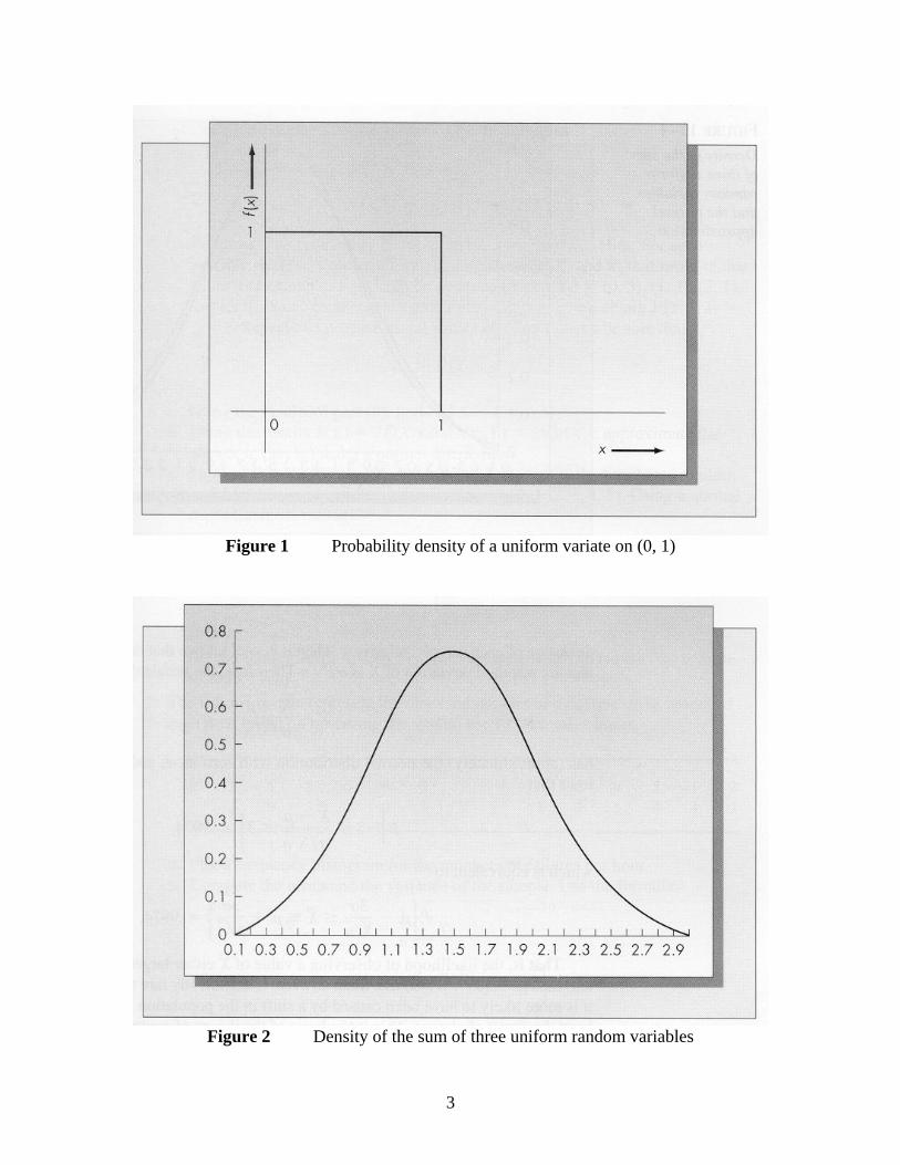
acceptance of SPC and other quality management initiatives. Important additions were made to quality control theory and practice, especially Motorola’s six-sigma controllability methodology (discussed below). It is ironic that a brilliant American invention was not accepted by American industries until threatened by Japanese competition making good use of that invention. 2.2. Statistical Basis of Control Charts Control charts provide a simple graphical means of monitoring a process in real time. Today, they have gained wide acceptance in industry – you would be hard-pressed to find a volume manufacturing plant producing technologically advanced products anywhere in the world that is not using SPC extensively. A control chart maps the output of a production process over time and signals when a change in the probability distribution generating observations seems to have occurred. To construct a control chart one uses information about the probability distribution of process variation and fundamental results from probability theory. Most types of control charts are based on the Central Limit Theorem of statistics. Roughly speaking, the central limit theorem says that the distribution of a sum of independent and identically distributed (IID) random variables approaches the normal distribution as the number of terms in the sum increases. Generally, the distribution of the sum converges very quickly to a normal distribution. For example, consider a random variable with a uniform distribution on the interval (0, 1). See Figure 1. Now assume the three random variables X1, X2, and X3 are independent, each of which has the uniform distribution on the interval (0, 1). Consider the random variable W = X1 + X2 + X3. If one plots the distribution of W, it tracks remarkably close to a normal distribution with the same mean and variance. See Figure 2. If we were to continue to add independent random variables, the agreement would be even closer. If (X1, X2, … , Xn) is a random sample, the sample mean is defined as

.1

1

n

iiX

nX

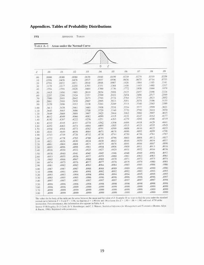
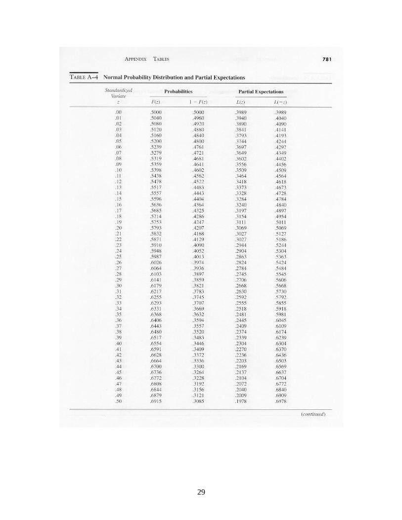
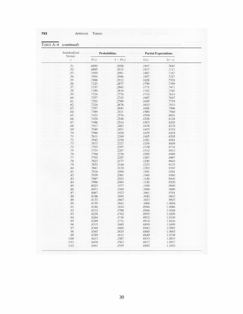
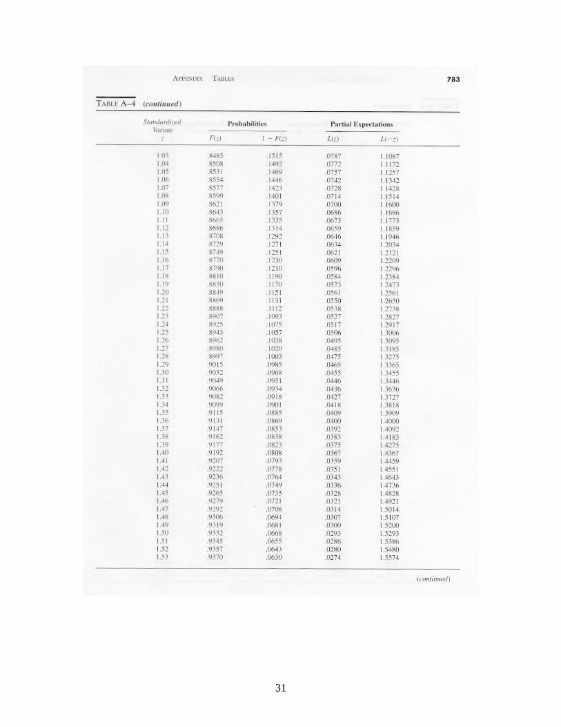
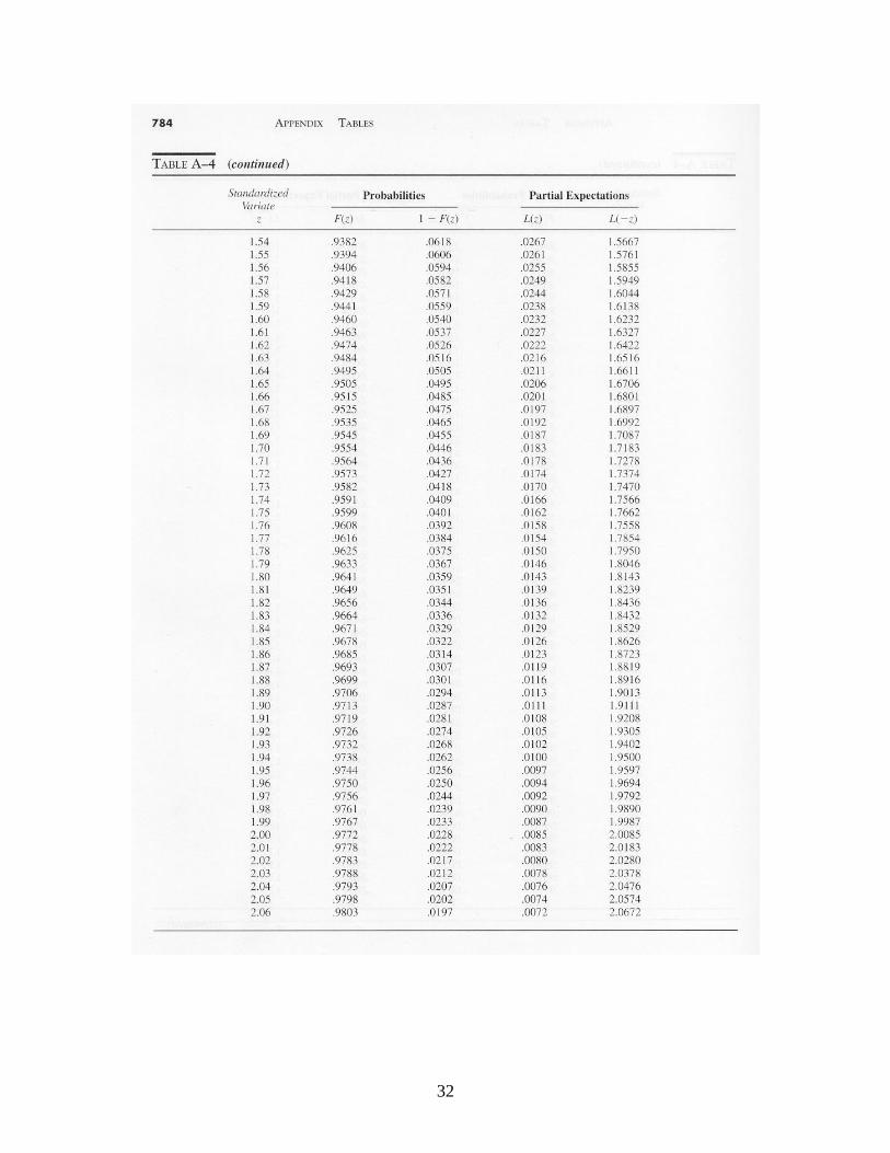
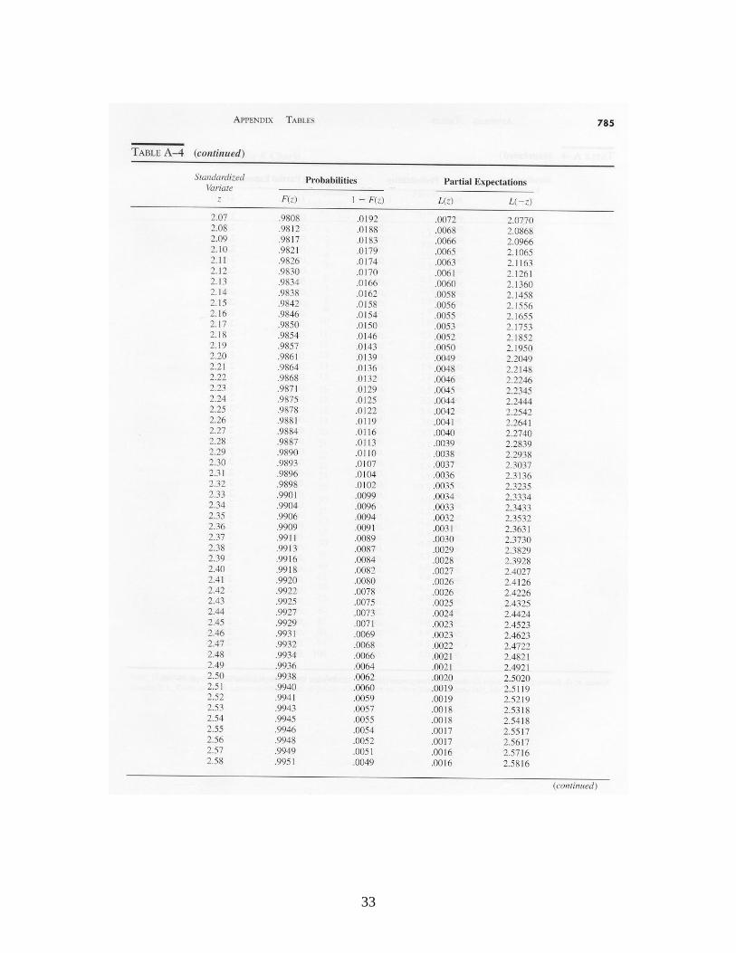
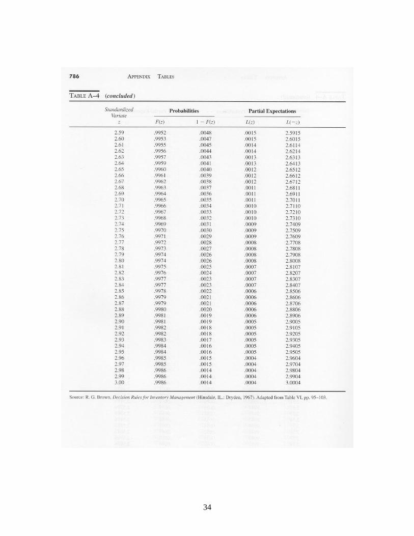
The Central Limit Theorem tells us that, regardless of the distribution of Xi, the sample mean will have a normal distribution, provided the variables are IID. Suppose that a random variable Z has the standard normal distribution (i.e., mean 0 and variance 1). Then, according to Table A-1,

.9974.033 ZP

3

Figure 1 Probability density of a uniform variate on (0, 1)

Figure 2 Density of the sum of three uniform random variables

4

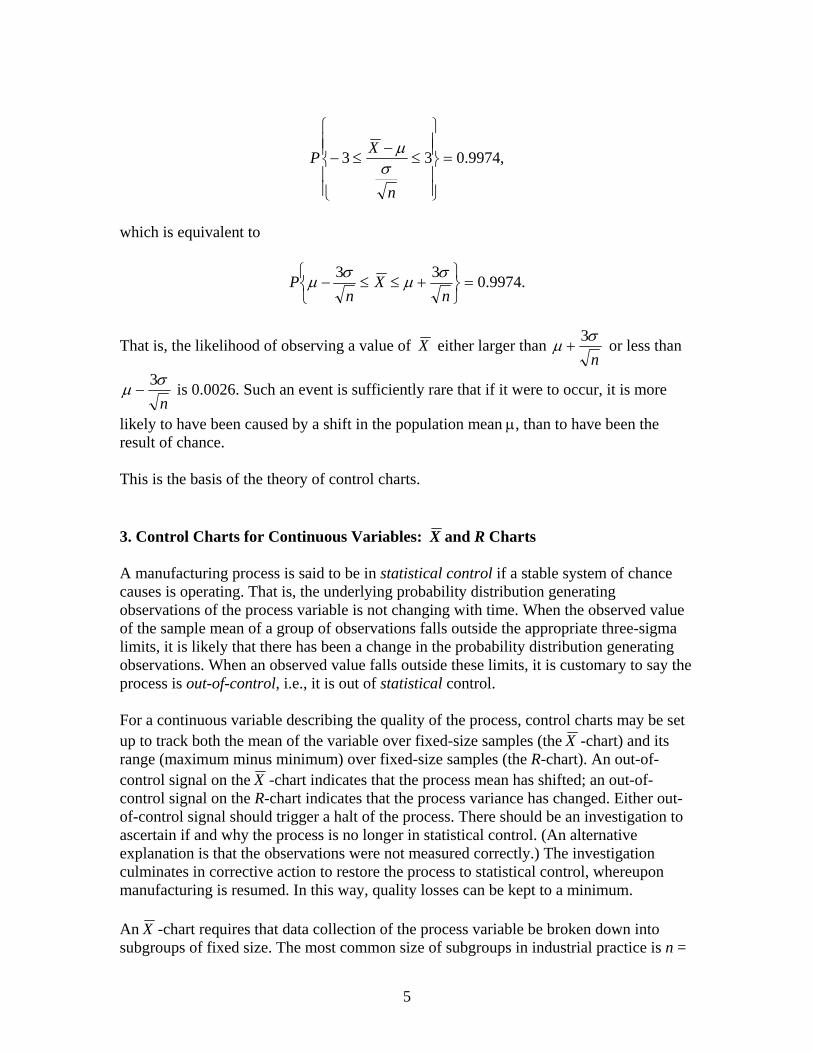
In other words, the likelihood of obtaining a value of Z either larger than 3 or less than -3 is 0.0026, or roughly 3 chances in 1,000. If such a value of Z is encountered, it is more likely that the IID assumption has been violated, i.e., there has been a drift or shift of the process that needs to be corrected. This is the basis of the so-called three-sigma limits that have become the de facto standard in SPC. Now consider the sample mean X . The Central Limit Theorem tells us it is (approximately) normally distributed. Suppose the mean of each sample is and the standard deviation is . The mean of X is expressed as

.)(11111

1111

nnn

EXn

XEn

Xn

EXEn

i

n

ii

n

ii

n

ii

The variance of X is derived as follows:

.11

12

1

n

ii

n

ii XVar

nX

nVarXVar

Now

,2

1

nXVarnXVar i

n

ii

so therefore

,2

nXVar

and the standard deviation of X is

.n

Therefore, the standardized variate

n

XZ

has (approximately) the normal distribution with mean zero and unit variance. It follows that

5

,9974.033

n

XP

which is equivalent to

.9974.033

n

Xn

P

That is, the likelihood of observing a value of X either larger than n

3 or less than

n

3 is 0.0026. Such an event is sufficiently rare that if it were to occur, it is more

likely to have been caused by a shift in the population mean , than to have been the result of chance. This is the basis of the theory of control charts. 3. Control Charts for Continuous Variables: X and R Charts A manufacturing process is said to be in statistical control if a stable system of chance causes is operating. That is, the underlying probability distribution generating observations of the process variable is not changing with time. When the observed value of the sample mean of a group of observations falls outside the appropriate three-sigma limits, it is likely that there has been a change in the probability distribution generating observations. When an observed value falls outside these limits, it is customary to say the process is out-of-control, i.e., it is out of statistical control. For a continuous variable describing the quality of the process, control charts may be set up to track both the mean of the variable over fixed-size samples (the X -chart) and its range (maximum minus minimum) over fixed-size samples (the R-chart). An out-of-control signal on the X -chart indicates that the process mean has shifted; an out-of-control signal on the R-chart indicates that the process variance has changed. Either out-of-control signal should trigger a halt of the process. There should be an investigation to ascertain if and why the process is no longer in statistical control. (An alternative explanation is that the observations were not measured correctly.) The investigation culminates in corrective action to restore the process to statistical control, whereupon manufacturing is resumed. In this way, quality losses can be kept to a minimum. An X -chart requires that data collection of the process variable be broken down into subgroups of fixed size. The most common size of subgroups in industrial practice is n =

6

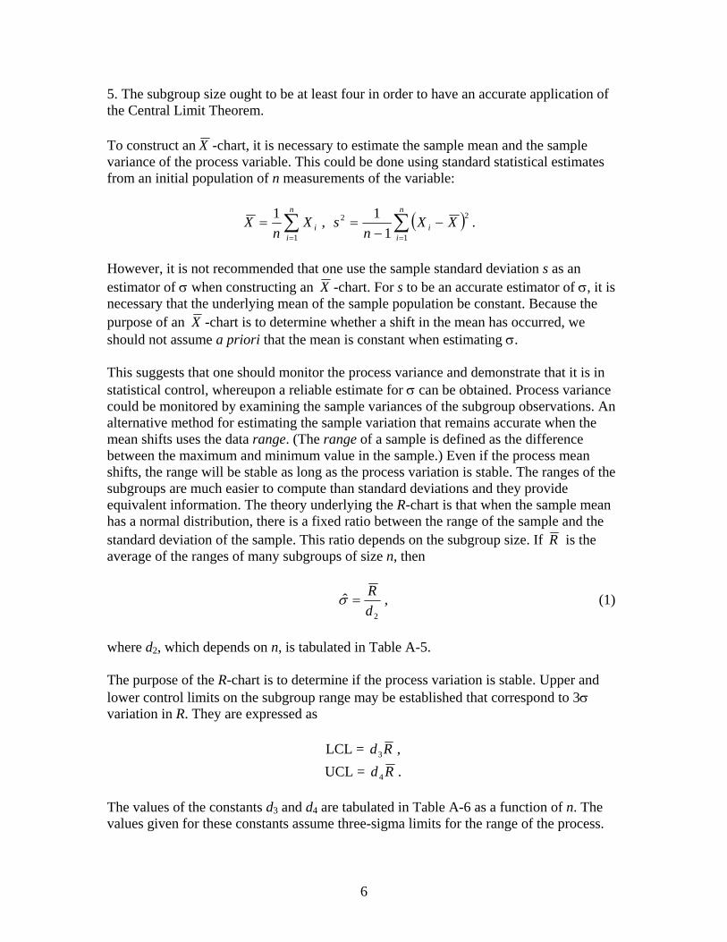
5. The subgroup size ought to be at least four in order to have an accurate application of the Central Limit Theorem. To construct an X -chart, it is necessary to estimate the sample mean and the sample variance of the process variable. This could be done using standard statistical estimates from an initial population of n measurements of the variable:

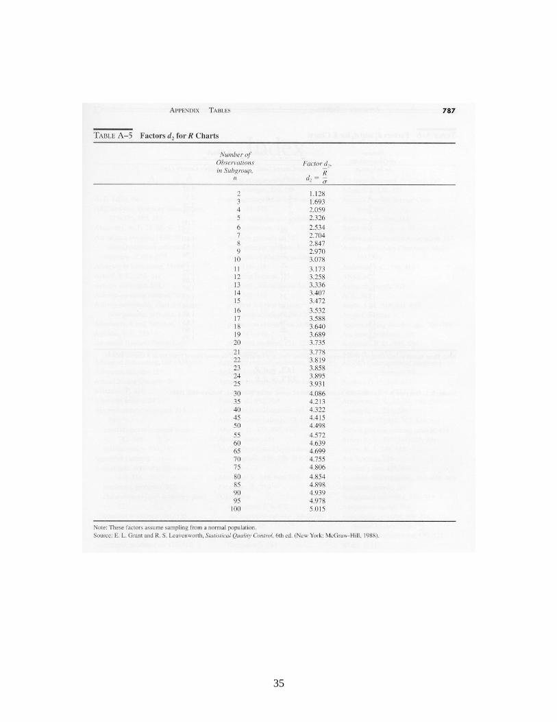
However, it is not recommended that one use the sample standard deviation s as an estimator of when constructing an X -chart. For s to be an accurate estimator of , it is necessary that the underlying mean of the sample population be constant. Because the purpose of an X -chart is to determine whether a shift in the mean has occurred, we should not assume a priori that the mean is constant when estimating . This suggests that one should monitor the process variance and demonstrate that it is in statistical control, whereupon a reliable estimate for can be obtained. Process variance could be monitored by examining the sample variances of the subgroup observations. An alternative method for estimating the sample variation that remains accurate when the mean shifts uses the data range. (The range of a sample is defined as the difference between the maximum and minimum value in the sample.) Even if the process mean shifts, the range will be stable as long as the process variation is stable. The ranges of the subgroups are much easier to compute than standard deviations and they provide equivalent information. The theory underlying the R-chart is that when the sample mean has a normal distribution, there is a fixed ratio between the range of the sample and the standard deviation of the sample. This ratio depends on the subgroup size. If R is the average of the ranges of many subgroups of size n, then

,ˆ2d

R (1)

where d2, which depends on n, is tabulated in Table A-5. The purpose of the R-chart is to determine if the process variation is stable. Upper and lower control limits on the subgroup range may be established that correspond to 3 variation in R. They are expressed as

LCL = ,3Rd

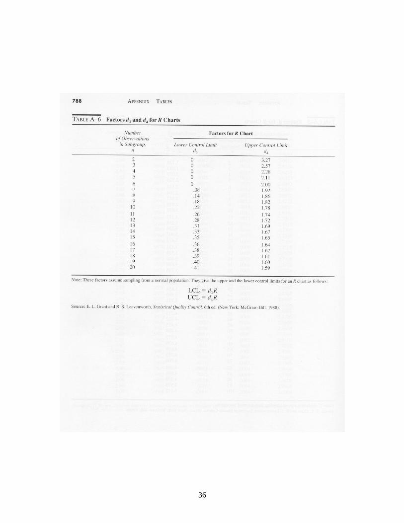
UCL = .4 Rd The values of the constants d3 and d4 are tabulated in Table A-6 as a function of n. The values given for these constants assume three-sigma limits for the range of the process.

.1

1,

1

1

22

1

n

ii

n

ii XX

nsX

nX

7

Typically, the R-chart is set up first in order to demonstrate that the process variance is stable and therefore obtain a reliable estimate of . If the range is found to be in statistical control across a reasonably long series of samples, then formula (1) above may be used to estimate the standard deviation. Given reliable estimators for the mean and standard deviation of the process, the X control chart is then constructed in the following way: Lines are drawn for the upper and

lower control limits at nX /3 . (Note that the “three-sigma” limits are drawn at 3

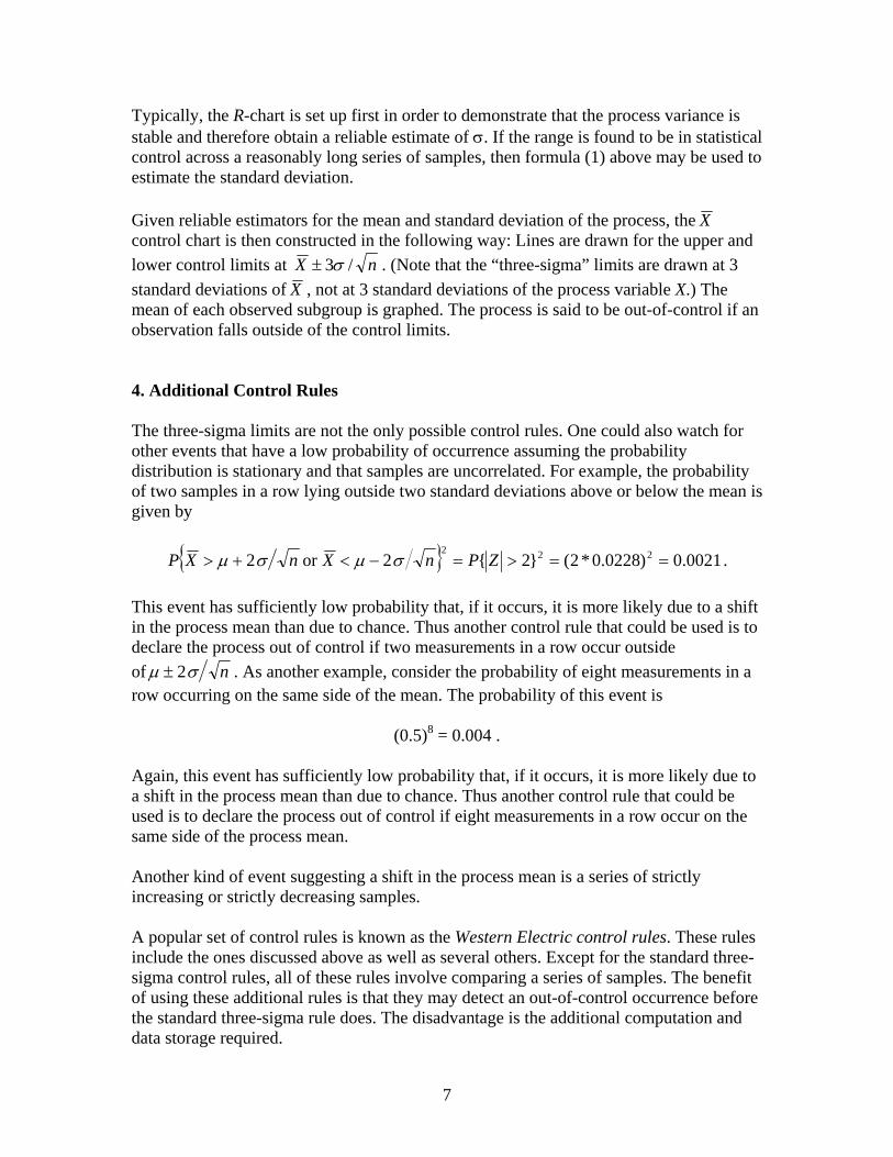
standard deviations of X , not at 3 standard deviations of the process variable X.) The mean of each observed subgroup is graphed. The process is said to be out-of-control if an observation falls outside of the control limits. 4. Additional Control Rules The three-sigma limits are not the only possible control rules. One could also watch for other events that have a low probability of occurrence assuming the probability distribution is stationary and that samples are uncorrelated. For example, the probability of two samples in a row lying outside two standard deviations above or below the mean is given by

.0021.0)0228.0*2(}2{2or 2 222 ZPnXnXP

This event has sufficiently low probability that, if it occurs, it is more likely due to a shift in the process mean than due to chance. Thus another control rule that could be used is to declare the process out of control if two measurements in a row occur outside

of n 2 . As another example, consider the probability of eight measurements in a row occurring on the same side of the mean. The probability of this event is

(0.5)8 = 0.004 .

Again, this event has sufficiently low probability that, if it occurs, it is more likely due to a shift in the process mean than due to chance. Thus another control rule that could be used is to declare the process out of control if eight measurements in a row occur on the same side of the process mean. Another kind of event suggesting a shift in the process mean is a series of strictly increasing or strictly decreasing samples. A popular set of control rules is known as the Western Electric control rules. These rules include the ones discussed above as well as several others. Except for the standard three-sigma control rules, all of these rules involve comparing a series of samples. The benefit of using these additional rules is that they may detect an out-of-control occurrence before the standard three-sigma rule does. The disadvantage is the additional computation and data storage required.

8

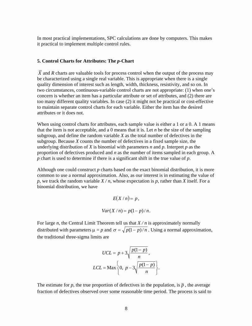
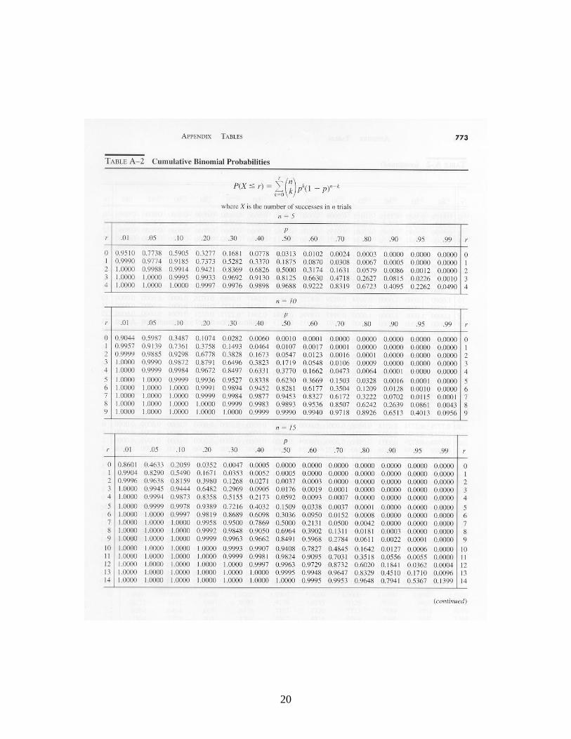
In most practical implementations, SPC calculations are done by computers. This makes it practical to implement multiple control rules. 5. Control Charts for Attributes: The p-Chart X and R charts are valuable tools for process control when the output of the process may be characterized using a single real variable. This is appropriate when there is a single quality dimension of interest such as length, width, thickness, resistivity, and so on. In two circumstances, continuous-variable control charts are not appropriate: (1) when one’s concern is whether an item has a particular attribute or set of attributes, and (2) there are too many different quality variables. In case (2) it might not be practical or cost-effective to maintain separate control charts for each variable. Either the item has the desired attributes or it does not. When using control charts for attributes, each sample value is either a 1 or a 0. A 1 means that the item is not acceptable, and a 0 means that it is. Let n be the size of the sampling subgroup, and define the random variable X as the total number of defectives in the subgroup. Because X counts the number of defectives in a fixed sample size, the underlying distribution of X is binomial with parameters n and p. Interpret p as the proportion of defectives produced and n as the number of items sampled in each group. A p chart is used to determine if there is a significant shift in the true value of p. Although one could construct p charts based on the exact binomial distribution, it is more common to use a normal approximation. Also, as our interest is in estimating the value of p, we track the random variable X / n, whose expectation is p, rather than X itself. For a binomial distribution, we have

,/ pnXE

./)1()/( nppnXVar

For large n, the Central Limit Theorem tell us that X / n is approximately normally

distributed with parameters = p and npp /)1( . Using a normal approximation,

the traditional three-sigma limits are

,)1(

3n

pppUCL

.)1(

3,0Max

n

pppLCL

The estimate for p, the true proportion of defectives in the population, is p , the average fraction of defectives observed over some reasonable time period. The process is said to

9

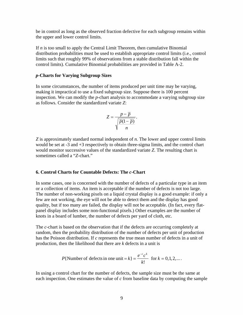
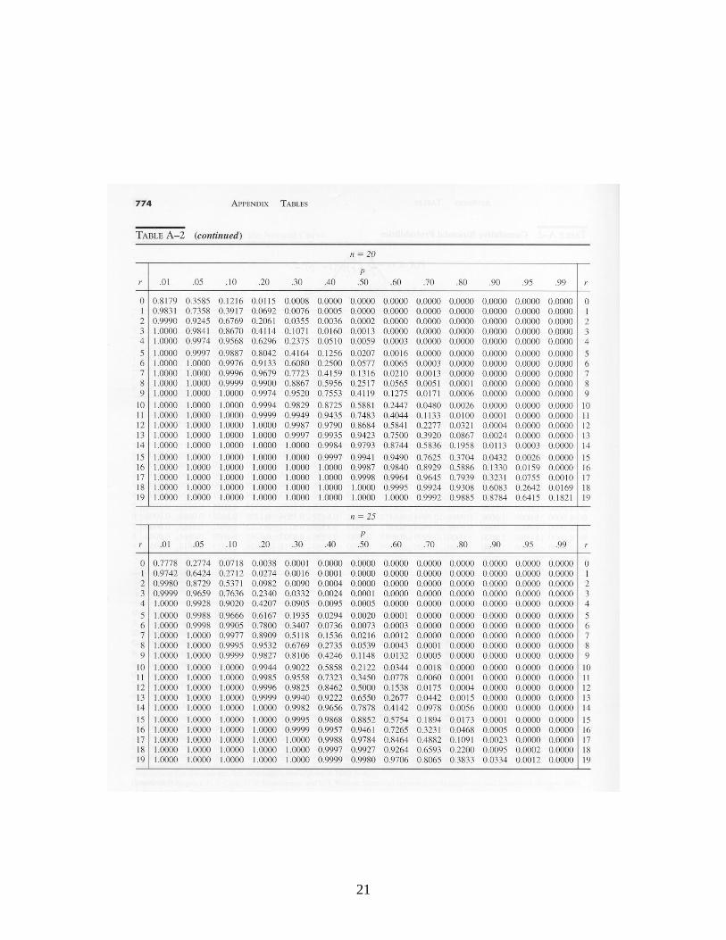
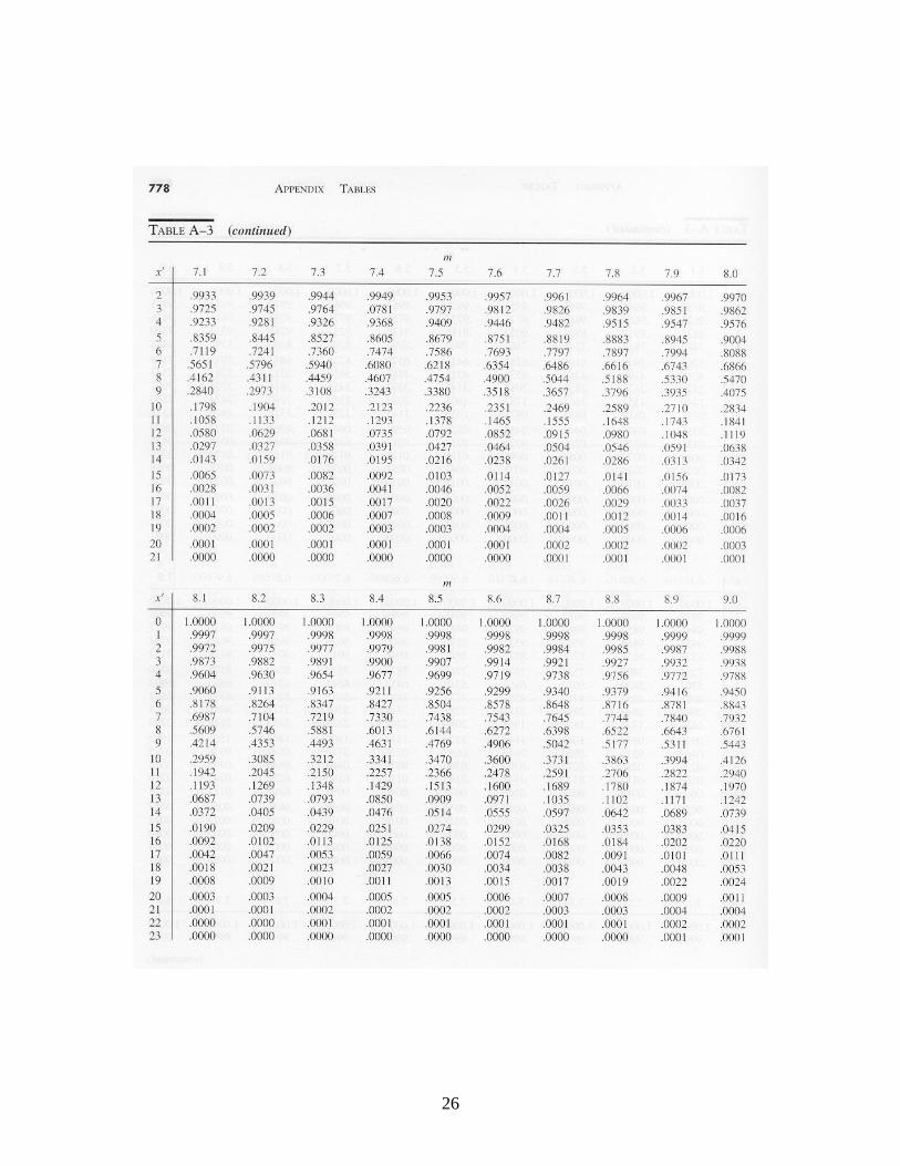
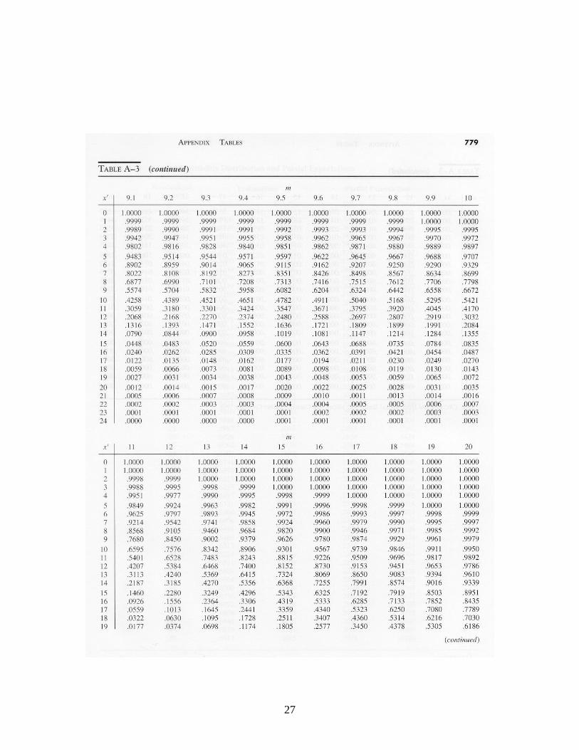
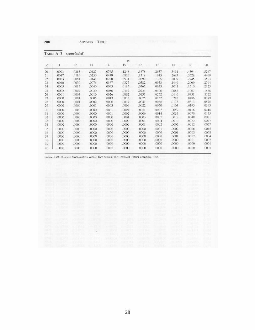
be in control as long as the observed fraction defective for each subgroup remains within the upper and lower control limits. If n is too small to apply the Central Limit Theorem, then cumulative Binomial distribution probabilities must be used to establish appropriate control limits (i.e., control limits such that roughly 99% of observations from a stable distribution fall within the control limits). Cumulative Binomial probabilities are provided in Table A-2. p-Charts for Varying Subgroup Sizes In some circumstances, the number of items produced per unit time may be varying, making it impractical to use a fixed subgroup size. Suppose there is 100 percent inspection. We can modify the p-chart analysis to accommodate a varying subgroup size as follows. Consider the standardized variate Z:

.)1(

n

pp

ppZ

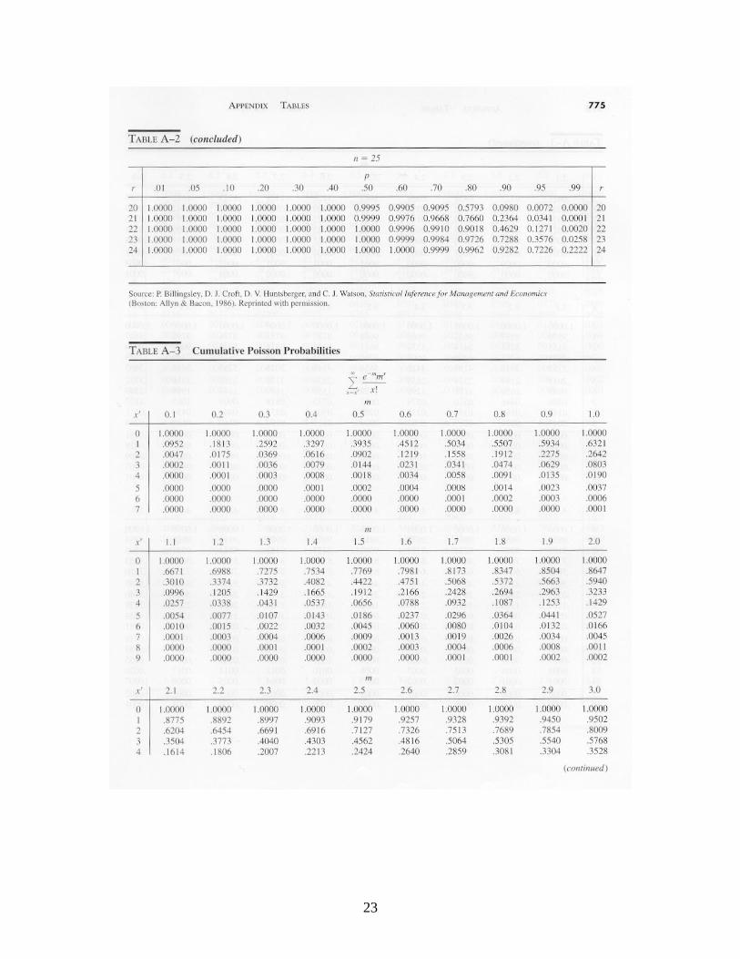
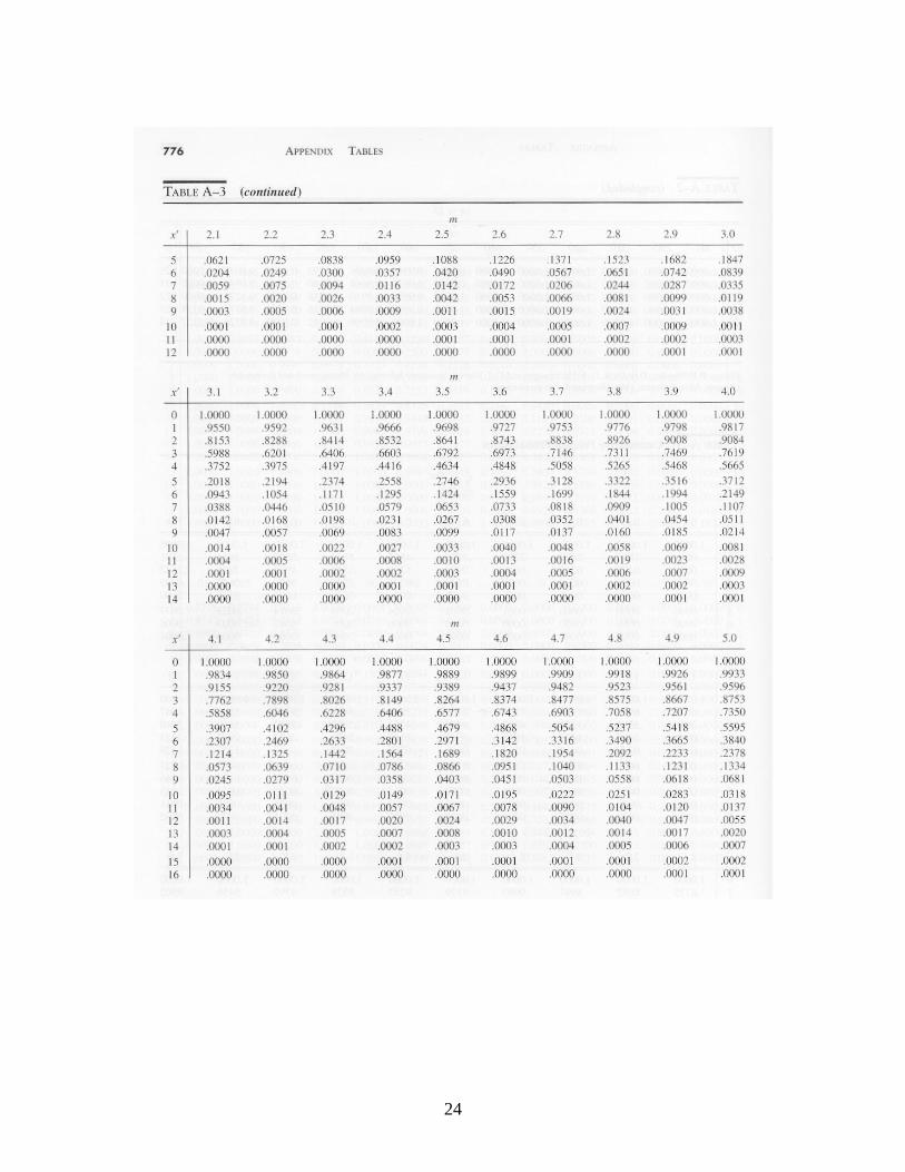
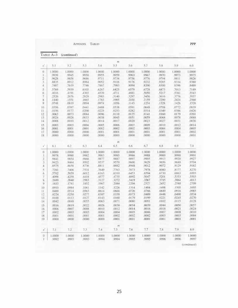
Z is approximately standard normal independent of n. The lower and upper control limits would be set at -3 and +3 respectively to obtain three-sigma limits, and the control chart would monitor successive values of the standardized variate Z. The resulting chart is sometimes called a “Z-chart.” 6. Control Charts for Countable Defects: The c-Chart In some cases, one is concerned with the number of defects of a particular type in an item or a collection of items. An item is acceptable if the number of defects is not too large. The number of non-working pixels on a liquid crystal display is a good example: if only a few are not working, the eye will not be able to detect them and the display has good quality, but if too many are failed, the display will not be acceptable. (In fact, every flat-panel display includes some non-functional pixels.) Other examples are the number of knots in a board of lumber, the number of defects per yard of cloth, etc. The c-chart is based on the observation that if the defects are occurring completely at random, then the probability distribution of the number of defects per unit of production has the Poisson distribution. If c represents the true mean number of defects in a unit of production, then the likelihood that there are k defects in a unit is

....,2,1,0for !

} unit onein defects ofNumber {

kk

cekP

kc

In using a control chart for the number of defects, the sample size must be the same at each inspection. One estimates the value of c from baseline data by computing the sample

10

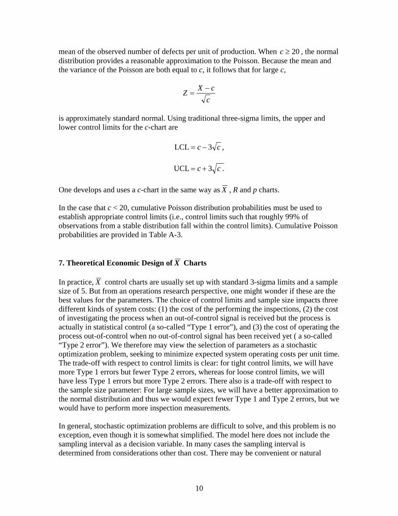
mean of the observed number of defects per unit of production. When 20c , the normal distribution provides a reasonable approximation to the Poisson. Because the mean and the variance of the Poisson are both equal to c, it follows that for large c,

c

cXZ

is approximately standard normal. Using traditional three-sigma limits, the upper and lower control limits for the c-chart are

,3LCL cc

.3 UCL cc

One develops and uses a c-chart in the same way as X , R and p charts. In the case that c < 20, cumulative Poisson distribution probabilities must be used to establish appropriate control limits (i.e., control limits such that roughly 99% of observations from a stable distribution fall within the control limits). Cumulative Poisson probabilities are provided in Table A-3. 7. Theoretical Economic Design of X Charts In practice, X control charts are usually set up with standard 3-sigma limits and a sample size of 5. But from an operations research perspective, one might wonder if these are the best values for the parameters. The choice of control limits and sample size impacts three different kinds of system costs: (1) the cost of the performing the inspections, (2) the cost of investigating the process when an out-of-control signal is received but the process is actually in statistical control (a so-called “Type 1 error”), and (3) the cost of operating the process out-of-control when no out-of-control signal has been received yet ( a so-called “Type 2 error”). We therefore may view the selection of parameters as a stochastic optimization problem, seeking to minimize expected system operating costs per unit time. The trade-off with respect to control limits is clear: for tight control limits, we will have more Type 1 errors but fewer Type 2 errors, whereas for loose control limits, we will have less Type 1 errors but more Type 2 errors. There also is a trade-off with respect to the sample size parameter: For large sample sizes, we will have a better approximation to the normal distribution and thus we would expect fewer Type 1 and Type 2 errors, but we would have to perform more inspection measurements. In general, stochastic optimization problems are difficult to solve, and this problem is no exception, even though it is somewhat simplified. The model here does not include the sampling interval as a decision variable. In many cases the sampling interval is determined from considerations other than cost. There may be convenient or natural

11

times to sample based on the nature of the process, the items being produced, or personnel constraints. The three costs we do consider are defined as follows: 1. Sampling cost. We assume exactly n items are sampled each period. (A “period” in this context might refer to a duration such as a production shift or to a production run quantity such as a manufacturing lot.) In many cases, sampling consumes workers’ time, so that personnel costs are incurred. There also may be costs associated with the equipment required for sampling. In some cases, sampling may require destructive testing, adding the cost of the item itself. We will assume that for each item sampled, there is a cost of a1. It follows that the sampling cost incurred each period is a1n. 2. Search cost. When an out-of-control condition is signaled, the presumption is that there is an assignable cause for the condition. The search for an assignable cause generally will require that the process be shut down. When an out-of-control signal occurs, there are two possibilities: either the process is truly out of control or the signal is a false alarm. In either case, we will assume that there is a cost a2 incurred each time a search is required for an assignable cause of the out-of-control condition. The search cost could include the costs of shutting down the facility, engineering time required to identify the cause of the signal, time required to determine of the out-of-control signal was a false alarm, and the cost of testing and possibly adjusting the equipment. Note that the search cost is probably a random variable; it might not be possible to predict the degree of effort required to search for an assignable cause of the out-of-control signal. When this is the case, interpret a2 as the expected search cost. 3. Operating out of control. The third and final cost we consider is the cost of operating the process after it has gone out of control. There is a greater likelihood that defective items are produced if the process is out of control. If defectives are discovered during inspection, they would either be scrapped or reworked. An even more serious consequence is that the defective item becomes part of a larger subassembly which must be disassembled or scrapped. Finally, defective items can make their way into the marketplace, resulting in possible costs of warranty claims, liability suits, and overall customer dissatisfaction. Assume that there is a cost a3 each period that the process is operated in an out-of-control condition. We consider the economic design of an X chart only. Assume that the process mean is and that the process standard deviation is . A sufficient history of observations is assumed to exist so that and can be estimated accurately. We also assume that an out-of-control condition means that the underlying mean undergoes a shift from to + or to – . Hence, out of control means that the process mean shifts by standard deviations. Define a cycle as the time interval from the start of production just after an adjustment to detection and elimination of the next out-of-control condition. A cycle consists of two parts. Define T as the number of periods that the process remains in control directly following an adjustment and S as the number of periods the process remains out of

12

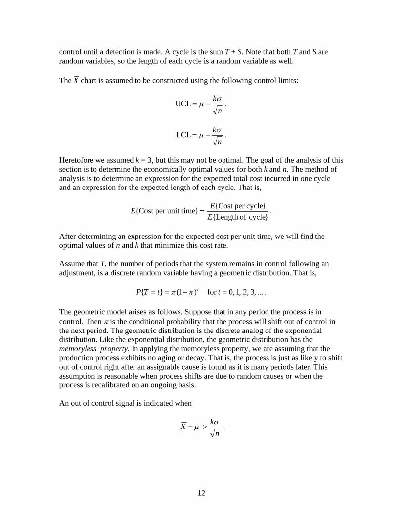
control until a detection is made. A cycle is the sum T + S. Note that both T and S are random variables, so the length of each cycle is a random variable as well. The X chart is assumed to be constructed using the following control limits:

, UCLn

k

. LCLn

k

Heretofore we assumed k = 3, but this may not be optimal. The goal of the analysis of this section is to determine the economically optimal values for both k and n. The method of analysis is to determine an expression for the expected total cost incurred in one cycle and an expression for the expected length of each cycle. That is,

.}cycle ofLength {

}cycleper Cost {}unit timeper Cost {

E

EE

After determining an expression for the expected cost per unit time, we will find the optimal values of n and k that minimize this cost rate. Assume that T, the number of periods that the system remains in control following an adjustment, is a discrete random variable having a geometric distribution. That is,

....,3,2,1,0for )1(}{ ttTP t

The geometric model arises as follows. Suppose that in any period the process is in control. Then is the conditional probability that the process will shift out of control in the next period. The geometric distribution is the discrete analog of the exponential distribution. Like the exponential distribution, the geometric distribution has the memoryless property. In applying the memoryless property, we are assuming that the production process exhibits no aging or decay. That is, the process is just as likely to shift out of control right after an assignable cause is found as it is many periods later. This assumption is reasonable when process shifts are due to random causes or when the process is recalibrated on an ongoing basis. An out of control signal is indicated when

.n

kX

13

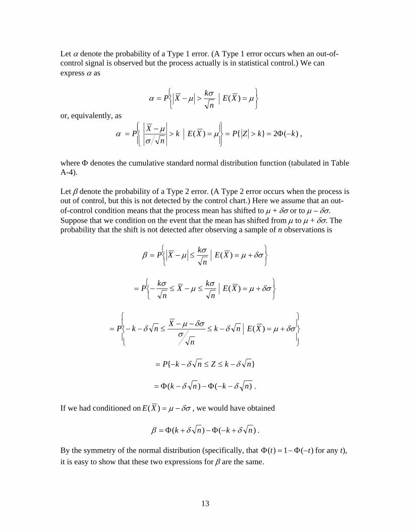
Let denote the probability of a Type 1 error. (A Type 1 error occurs when an out-of-control signal is observed but the process actually is in statistical control.) We can express as

)(XEn

kXP

or, equivalently, as

,)(2}{)( kkZPXEkn

XP

where denotes the cumulative standard normal distribution function (tabulated in Table A-4). Let denote the probability of a Type 2 error. (A Type 2 error occurs when the process is out of control, but this is not detected by the control chart.) Here we assume that an out-of-control condition means that the process mean has shifted to + or to – . Suppose that we condition on the event that the mean has shifted from to + . The probability that the shift is not detected after observing a sample of n observations is

)(XEn

kXP

)(XE

n

kX

n

kP

)(XEnk

n

XnkP

}{ nkZnkP

.)()( nknk

If we had conditioned on )(XE , we would have obtained

.)()( nknk

By the symmetry of the normal distribution (specifically, that )(1)( tt for any t),

it is easy to show that these two expressions for are the same.

14

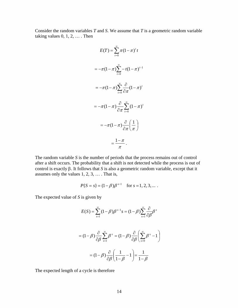
Consider the random variables T and S. We assume that T is a geometric random variable taking values 0, 1, 2, … . Then

0

)1()(t

t tTE

0

1)1()1(t

tt

t

t

)1()1(0

0

)1()1(t

t

1)1(

.1

The random variable S is the number of periods that the process remains out of control after a shift occurs. The probability that a shift is not detected while the process is out of control is exactly . It follows that S is also a geometric random variable, except that it assumes only the values 1, 2, 3, … . That is,

. ... 3, 2, 1, for )1(}{ 1 ssSP s

The expected value of S is given by

s

ss

s sSE

11

1 )1()1()(

1)1()1(01 s

s

s

s

1

11

1

1)1(

The expected length of a cycle is therefore

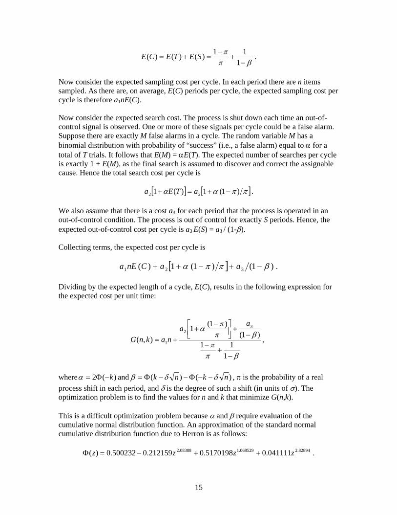
15

.1

11)()()(

SETECE

Now consider the expected sampling cost per cycle. In each period there are n items sampled. As there are, on average, E(C) periods per cycle, the expected sampling cost per cycle is therefore a1nE(C). Now consider the expected search cost. The process is shut down each time an out-of-control signal is observed. One or more of these signals per cycle could be a false alarm. Suppose there are exactly M false alarms in a cycle. The random variable M has a binomial distribution with probability of “success” (i.e., a false alarm) equal to for a total of T trials. It follows that E(M) = E(T). The expected number of searches per cycle is exactly 1 + E(M), as the final search is assumed to discover and correct the assignable cause. Hence the total search cost per cycle is

.)1(1)(1 22 aTEa

We also assume that there is a cost a3 for each period that the process is operated in an out-of-control condition. The process is out of control for exactly S periods. Hence, the expected out-of-control cost per cycle is a3 E(S) = a3 / (1-). Collecting terms, the expected cost per cycle is

.)1()1(1)( 321 aaCnEa

Dividing by the expected length of a cycle, E(C), results in the following expression for the expected cost per unit time:

,

1

11)1(

)1(1

),(

32

1

aa

naknG

where )()( and )(2 nknkk , is the probability of a real

process shift in each period, and is the degree of such a shift (in units of ). The optimization problem is to find the values for n and k that minimize G(n,k). This is a difficult optimization problem because and require evaluation of the cumulative normal distribution function. An approximation of the standard normal cumulative distribution function due to Herron is as follows:

.041111.05170198.0212159.0500232.0)( 82894.2068529.108388.2 zzzz

16

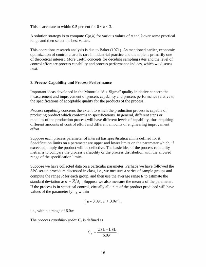
This is accurate to within 0.5 percent for 0 < z < 3. A solution strategy is to compute G(n,k) for various values of n and k over some practical range and then select the best values. This operations research analysis is due to Baker (1971). As mentioned earlier, economic optimization of control charts is rare in industrial practice and the topic is primarily one of theoretical interest. More useful concepts for deciding sampling rates and the level of control effort are process capability and process performance indices, which we discuss next. 8. Process Capability and Process Performance Important ideas developed in the Motorola “Six-Sigma” quality initiative concern the measurement and improvement of process capability and process performance relative to the specifications of acceptable quality for the products of the process. Process capability concerns the extent to which the production process is capable of producing product which conforms to specifications. In general, different steps or modules of the production process will have different levels of capability, thus requiring different amounts of control effort and different amounts of engineering improvement effort. Suppose each process parameter of interest has specification limits defined for it. Specification limits on a parameter are upper and lower limits on the parameter which, if exceeded, imply the product will be defective. The basic idea of the process capability metric is to compare the process variability or the process distribution with the allowed range of the specification limits. Suppose we have collected data on a particular parameter. Perhaps we have followed the SPC set-up procedure discussed in class, i.e., we measure a series of sample groups and compute the range R for each group, and then use the average range R to estimate the standard deviation as 2dR . Suppose we also measure the mean of the parameter. If the process is in statistical control, virtually all units of the product produced will have values of the parameter lying within

[ - 3.0 , + 3.0 ] , i.e., within a range of 6.0. The process capability index Cp is defined as

,0.6

LSLUSL

pC

17

where USL is the upper specification limit and LSL is the lower specification limit. Suppose Cp = 1.0. If the mean was located exactly half way between USL and LSL, we would get very few defective units of product, and one might think that in that case we have high process capability. But if the mean drifts even a little, the number of defectives will start to climb up from 0. As a practical matter, it is not realistic to expect to hold the process mean exactly constant, so a value of 1.0 does not really represent all that high a process capability. On the other hand, a Cp value less than one is unsatisfactory -- clearly, there will be a significant number of defective units, and so we have low capability in that case. In general, a Cp value between 1.0 and 1.60 shows medium capability, and a Cp value of more than 1.60 shows high capability. The process capability index does not measure how centered is the process distribution relative to the specification limits. The process might have a high process capability index (i.e., a low relative variability), but if it is centered close to one of the specification limits, there still could be many defective units produced. For this reason, another metric is useful, known as the process performance index. The process performance index Cpk is defined as

.0.3

LSL,

0.3

USLMin

pkC

The idea is, we should try to keep the mean more than three standard deviations from the nearest specification limit -- that way, we avoid producing defective units. As before, we would like to stay more than 3.0 away from the nearest spec limit, so that there is room for the process to drift without cause for concern. A commonly cited industry goal is to drive Cpk for all process parameters up to a value of 1.33 or higher. If Cpk of a particular parameter becomes quite large, it suggests that sampling can be done less frequently, or perhaps it even becomes unnecessary. On the other hand, parameters with low values of Cpk need the most attention. Frequent sampling is necessary to avoid production of defects, and fundamental process improvements to achieve less variability are urgently needed. A very common case in industry is to have a one-sided specification limit, as when the number of particles must not exceed a given number. The process capability index has no meaning in this case, and it is not correct to use zero or some artificial specification limit in order to apply the formula. However, the process performance index in this case is readily defined. For the case of only an upper specification limit,

.0.3

USL

pkC

Acknowledgements

18

Sections 2, 3, 5, 6 and 7 of this chapter are adapted from Nahmias (2001). Bibliography Baker, Kenneth R. (1971). “Two Process Models in the Economic Design of an X Chart,” AIIE Transactions, 13 (1971), pp. 257-63. Nahmias, Steven (2001). Production and Operations Analysis, fourth edition, McGraw Hill – Irwin, New York. Shewhart, Walter A. (1931). Economic Control of the Quality of Manufactured Product, D. Van Nostrand, New York.

19

Appendices. Tables of Probability Distributions

20

21

22

23

24

25

26

27

28

29

30

31

32

33

34

35

36