Due Date Quotation Models and Algorithms

Philip Kaminsky

Dorit Hochbaum

Industrial Engineering and Operations Research

University of California, Berkeley, CA

September 2003

1 Introduction

When firms operate in a make-to-order environment, they must set due dates (or lead times)

which are both relatively soon in the future and can be met reliably in order to compete

effectively. This can be a difficult task, since there is clearly an inherent tradeoff between

short due dates, and due dates that can be easily met. Nevertheless, the vast majority of

due date scheduling research assumes that due dates for individual jobs are exogenously

determined. Typically, scheduling models which involve due dates focus on sequencing jobs

at various stations in order to optimize some measure of the ability to meet the given due

dates. However, in practice, firms need an effective approach for quoting due dates, and for

sequencing jobs to meet these due dates. In this chapter, we consider a variety of models

that contain elements of this important and practical problem, which is often known as the

due date quotation and scheduling problem, or the due date management problem.

In this chapter, we focus on papers thatcontain analytical results, and describe the algo-

rithms and results presented in those papers in some detail. We do not discuss simulation-

based research, or papers that focus on industrial applications rather than theory. We will

follow many of the conventions of traditional scheduling theory, and assume our reader is

familiar with basic scheduling concepts. For a comprehensive description of due-date related

papers, including simulation-based research and descriptions of industrial applications, see

Keskinocak and Tayur [33]. We also refer the reader to Cheng and Gupta [15], an earlier

comprehensive survey of this area.

1

��

���

���

��

��

����

���

HHHH

HHj

-�

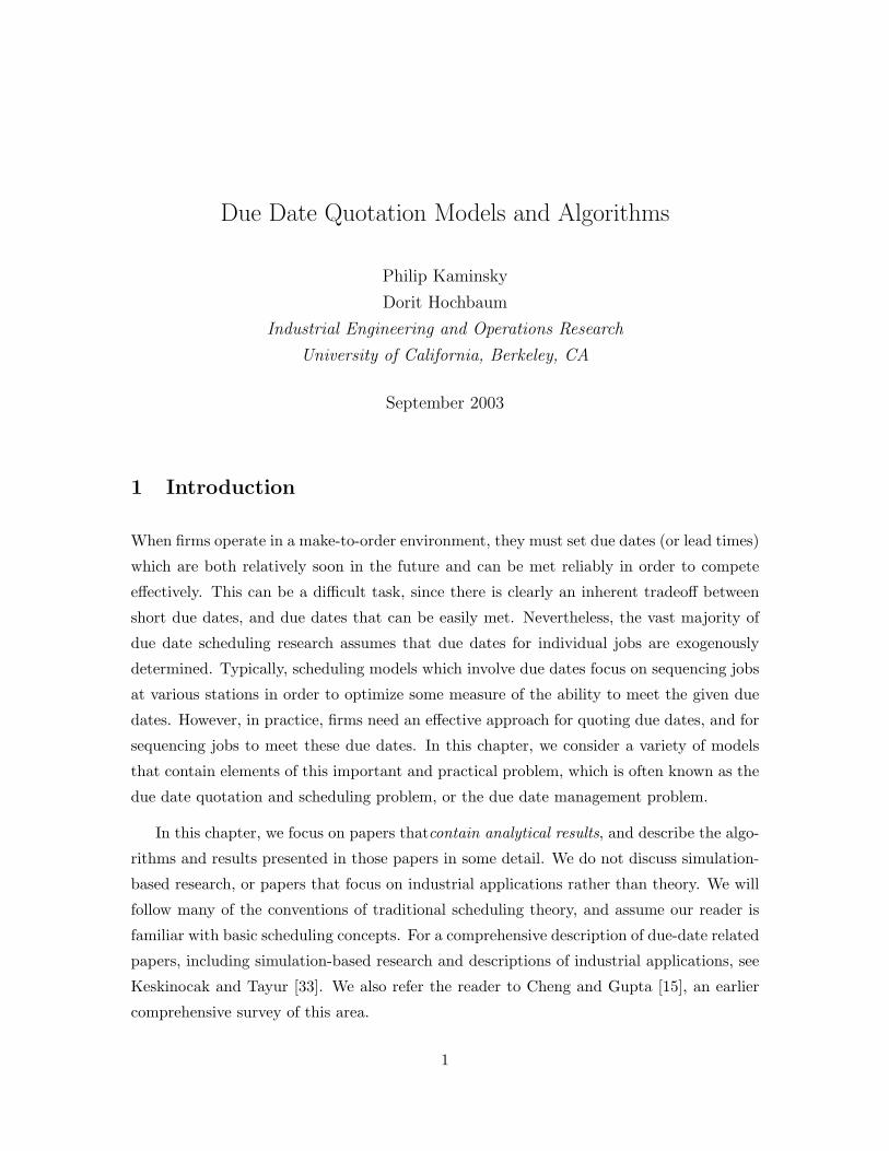
Capacity

Due dates Sequencing

Figure 1: Sequencing vs. Due Date Quotation

2 Overview

Most of the models discussed in this chapter contain two elements: a due-date setting ele-

ment, and a sequencing element. Since capacity is inherently limited in scheduling models,

it is frequently impossible to set ideal due dates, and to sequence jobs so that they com-

plete processing precisely at these ideal due dates. Indeed, the interplay between sequencing

jobs to meet due dates, and setting due dates so that sequencing is possible, makes these

problems very difficult (see Figure 1).

Ideally, of course, the sequencing and due date quotation problems will be solved si-

multaneously – rules or algorithms are developed that both quote due dates, and suggest

an effective sequence. Unfortunately, in many cases, solving these problems simultaneously

is difficult or impossible. In these cases, researchers turn either to sequenced-based models,

where some sequence or sequencing rule is selected, and then due dates are optimized based

on this sequence or rule, or due date-based models in which the due date is first assigned,

and then the sequence is set based on this due date. Frequently, the model or analysis ap-

proach dictates this choice. In queuing models, for example, the analysis frequently requires

a sequencing rule (such as first come, first served) to be selected, and then due dates to be

set based on this rule. Indeed, one can argue that in general the sequence-based approach

makes more sense, since the due date depends on the available capacity, which is directly

dependent upon how jobs are sequenced.

Much of the notation used in the chapter will be introduced as needed. Some of the

notation is fairly standard, however, and is introduced below. For job i,

• For any problem, there are N jobs, and M machines. Where appropriate, N and M

also refer to the set of jobs and machines. If the number of machines is not discussed,

2

it is assumed to be a single machine.

• ri represents the release time, or availability for processing, of the job.

• pi represents the processing time of the job. If the job is processed on more than one

machine, pmi represents the processing time of job i on machine m.

• Given a schedule, Ci represents the completion time of the job in that schedule.

• Given a due date quotation approach, di is the due date of job i in that schedule. If

the model under consideration is a common due date model, then d represents the

common due date.

• Given Ci and di, Ei represents the earliness of job i, max{di − Ci, 0}.

• Given Ci and di, Ti represents the tardiness of job i, max{Ci − di, 0}.

• The quoted lead time of a job is the time between its release and its due date, di − ri.

Sometimes models will be expressed in terms of quoted lead times rather than quoted

due dates. The flow time of a job is the actual time between its release time and its

completion, Ci − ri completion.

• Given a sequence of jobs, job j[i] is the ith job in the sequence, with processing time

p[i], release time r[i], etc.

The models considered in this chapter for the most part follow standard scheduling

convention. We consider single machine models, parallel machine models, job shops, and

flow shops, both dynamic (that is, jobs have different release or available times) and static

(that is, all jobs are available at the start of the horizon.) Some due date quotation models

don’t restrict the quoted due dates. In other words, any due date can be quoted for any

job. Some models are so-called common due date models. In these models, a single due

date must be quoted for all of the jobs.

Because it is sometimes impractical to quote due dates from an unrestricted set of

possible due dates, researchers have considered a variety of problem in which the class of

possible due dates is limited. In general, this research involves proposing a simple due date

setting rule, and then attempting to optimize the parameters of that rule in order to achieve

some objective. Three types of due date setting rules are commonly used:

3

• CON: jobs are given constant lead times, so that for job j, dj = rj + γ. Note that

for a static problem (with all release times equal), this is equivalent to a common due

date.

• SLK: jobs are given lead times that reflect equal slacks, so that for job j, dj =

rj + pj + β.

• TWK: jobs are assigned lead times proportional to their lengths (or their Total WorK),

so that dj = rj + αpj .

A variety of different sequencing and scheduling rules have been employed for these

types of models. Some standard dispatch rules include:

• Shortest Processing Time (SPT): jobs are sequenced in non-decreasing order of pro-

cessing times.

• Longest Processing Time (LPT): jobs are sequenced in non-increasing order of pro-

cessing times.

• Weighted Shortest Processing Time (WSPT) and Weighted Longest Processing Time

(WLPT): job i has an associated weight wi. For WSPT, jobs are sequenced in non-

decreasing order of pi/wi; for WLPT, jobs are sequenced in non-increasing order of

the same ratio.

• Earliest Due Date (EDD): jobs are sequenced in non-decreasing order of due dates.

We observe that for due date quotation problems, sequencing jobs EDD in some sense

removes a degree of freedom from the optimizer, since instead of making sequencing

and due date quotation decisions, for an EDD problem, the due date quotation directly

implies a sequence.

• Shortest Processing Time among Available jobs (SPTA): in a dynamic model, each

time a job completes processing, the next job to be processed is the shortest job in

the set of released but not yet processed jobs.

• Preemptive SPT (PSPT): in a dynamic model, each time a job is released, the current

job will be stopped, and the newly released job will be processed, if the remaining

processing time of the currently processing job is longer than the processing time

of the newly released job. When a job completes processing, the job with shortest

remaining processing time is processed.

4

• Preemptive EDD (PEDD): in a dynamic model, each time a job is released, the current

job will be stopped, and the newly released job will be processed, if the newly released

job has an earlier due date than the currently processing job. When a job completes

processing, the remaining job with the earliest due date will be processed.

Researchers have considered a variety of objectives for due date quotation models. Many

of them involve functions of quoted due date or due dates, and the earliness and tardiness

of sequenced jobs. In addition, some models feature reliability constraints. For example,

some models feature a 100% reliability constraint, which requires each job to complete by

its quoted due date. Some models feature probabilistic reliability constraints, which limits

the probability that a job will exceed its quoted due date. Some reliability constraints limit

the fraction of jobs that can be tardy, or the the total amount of tardiness.

The remainder of this chapter is organized as follows. Each section considers a class of

models: single machine common due date models, single machine static distinct due date

models, single machine dynamic models, parallel machine models, and jobshop and flowshop

models. Within each section, we introduce a variety of models, present their objectives, and

present analytical results and algorithms from the literature. The section on single machine

dynamic models is further divided into on-line and off-line models. In this context, on-

line scheduling algorithms sequence jobs at any time using only information pertaining to

jobs which have been released by that time. This models many real world problems, where

job information is not known until a job arrives, and information about future arrivals is

not known until these jobs arrive. In contrast, off-line algorithms may use information

about jobs which will be released in the future to make sequencing and due date quotation

decisions. The on-line section is further divided into subsections featuring probabilistic

analysis of heuristics, worst-case analysis of heuristics, and queuing-theory based analysis

of related models.

We conclude with a discussion of some models that don’t fit these categories, and discuss

research opportunities in this area.

3 Single Machine Static Common Due Date Models

In the models considered in this section, all jobs are assumed to be available at the start

of the scheduling horizon (a static problem, with ri = 0 for all jobs). Jobs must be pro-

cessed sequentially on a single machine, and processing times are deterministic (with a few

5

exceptions, described below) and known at the start of the scheduling horizon. We use d

to represent the common due date.

The most frequently explored objective for this class of models is a function of the

weighted sum of the due date, earliness and tardiness over all jobs. Each of these three

components is given a weight that can differ by job, so that the overall objective is thus∑Ni=1(π

di d+πe

i Ei +πtiTi) where πd

i , πei , πt

i , are the due date, earliness, and tardiness weights

associated with job i respectively. In standard three field scheduling notation, the model

can be expressed: 1|dopt|∑N

i=1(πdi d+πe

i Ei+πtiTi), where the notation dopt is used to indicate

that the due date is determined within the model, and not externally assigned.

Baker and Scudder [3] and Quaddus [39] analyzed the structure of this model. Observe

that ifn∑

i=1

πdi ≥

n∑i=1

πti (1)

then the optimal common due date d∗ = 0. To see this, notice that for any sequence,

increasing the due date from 0 will increase due date costs more than it decreases tardiness

costs if condition (1) is met. In addition, any increase in due dates can only increase earliness

cost. If condition (1) is met, all of the jobs will be tardy, so the total tardiness is minimized

by sequencing jobs in nondecreasing order of pi/πti . If condition (1) is not met, it is not

difficult to show that for any given sequence, the optimal schedule involves no inserted idle

time, and the optimal due date must be equal to the completion time of one of the jobs.

To see this, observe that if there is any idle time in the schedule, either the job im-

mediately preceding the idle time is early, and could be shifted later, decreasing the total

earliness penalty, or the job immediately after the idle is tardy, and could be shifted earlier,

decreasing the total tardiness. By repeatedly applying this observation, any schedule with

inserted idleness could be converted to a schedule without inserted idleness with a lower

objective function value. Now, suppose that jobs are contiguously scheduled, but that the

first job does not start processing at time 0, and instead starts processing at time T . If the

starting time of each of the jobs is decreased by T , and the due date is decreased by T ,

then earliness and tardiness costs will not change, but the due date cost will decrease by∑Ni=1 πd

i T .

Now, suppose that in such a schedule, the due date d does not coincide with the com-

pletion time of one of the jobs. If d < C[1], then no jobs are early and d can be increased by

δ to C[1]. In this case, the objective function will decrease by at least δ(∑n

i=1 πti −∑n

i=1 πdi ),

and since condition (1) is not met, this is a positive quantity. If d > C[N ], then no jobs are

6

tardy and d can be decreased to C[N ]. In this case, both earliness and due date costs will

decrease, and there will still be no tardiness costs, so the objective decreases.

Finally, suppose that for some job j, 1 ≤ j ≤ N − 1, C[j] < d < C[j+1]. Let F represent

the objective function value given d, and let x = d− C[i] and y = C[i+1] − d. Clearly, both

x > 0 and y > 0. If the due date is changed to C[i], the new objective Fi will equal:

Fi = F + x(N∑

j=1

(πti − πd

i )−i∑

j=1

((πei + πt

i)).

Similarly, if the due date is changed to C[i+1], the new objective Fi+1 will equal:

Fi+1 = F − y(N∑

j=1

(πti − πd

i )−i∑

j=1

((πei + πt

i)).

Clearly, if∑N

j=1(πti−πd

i )−∑i

j=1((πei +πt

i) is positive, then Fi+1 < F , and if it is negative,

then Fi < F .

Now, consider a given sequence, and two adjacent jobs, [j − 1] and [j]. Following Baker

and Scudder [3], we will compare two schedules, S, in which d = C[j−1], and S′, in which

d′ = C[j]. The objective function can be written:

f(S, d) =N∑

i=1

πd[i]d +

j−1∑i=1

πe[i](d− C[i]) +

N∑i=1

πt[i](C[i] − d).

Now, observing that

C[i] =i∑

k=1

p[k]

and

d =j−1∑k=1

p[k]

and substituting into the objective function, we get:

f(S, d) =j−1∑k=1

p[k]

(k−1∑i=1

πe[i] +

N∑i=1

πd[i]

)+

N∑k=j

p[k]

(N∑

i=k

πt[i]

).

Letting G(S, S′) = f(S, d)− f(S′, d′), we get:

G(S, S′) = p[j]

j−1∑k=1

πe[k] + p[j]

N∑k=1

πd[k] − p[j]

N∑k=j

πt[i]

7

Observe that S′ has a better objective value than S, and the due date should be later than

C[j−1], if:j−1∑k=1

(πe[k] + πt

[k]) <N∑

k=1

(πt[k] − πd

[k])

and that the due date should be no later than C[j] if the reverse is true. Therefore, for any

given sequence, we can conclude that the optimal due date d = C[r], where r is the smallest

integer for which:r∑

k=1

(πe[k] + πt

[k]) ≥N∑

k=1

(πt[k] − πd

[k]). (2)

Quaddus [39] provides an alternative proof of this result using duality theory.

Note that for any sequence, the jobs will be partitioned into two sets, one of on-time

jobs, and one of tardy jobs. Using a simple adjacent pairwise interchange proof, it can

be shown that the on-time jobs are scheduled WLPT (in non-increasing order of pi/πei ,

and the tardy jobs are scheduled WSPT (in non-decreasing order of pi/πti). This is known

as a V-shaped schedule, and this type of schedule is optimal for many related common

due date problems. (See Figure 2 for an example of a V-shaped sequence.) For example,

Raghavachari [41] uses an interchange argument to prove that the optimal sequence of jobs

around a common due date must be V-shaped,when the objective is to minimize the sum of

deviations around the due date (in other words, the problem described above, with πd = 0

and πe = πt).

-

6 u uu u u u

Completion Time

Processing

Time

1 2 3 4 5 6

due date

6

Figure 2: A V-Shaped Schedule

Hall and Posner [26] prove that 1|dopt|∑N

i=1(πdi d + πe

i Ei + πtiTi) is NP-Hard. Baker and

Scudder [3] propose an optimization procedure to find the optimal sequence that involves

enumerating V-shaped sequences and determining due dates and thus objective values as

described above.

8

Panwalker, Smith, and Seidmann [36] consider a special case of the model described

above, where earliness, tardiness, and the (single) due date are given weights that do not

differ by job. The overall objective is thus∑N

i=1(πdd + πeEi + πtTi).

As observed above, if πd ≥ πt, then d∗ = 0 and it is optimal to sequence jobs in SPT

order, and for any sequence, there is an optimal d value equal to the completion times of

one of the jobs.

For this version of the model, equation (2) can be simplified so that for any specified

sequence, there is an optimal due date C[r], where

r = dN πt − πd

πe + πte. (3)

Next, observe that given a sequence of jobs, the objective function can be rewritten

r∑j=1

(nπd + (j − 1)πe)p[j] +N∑

j=r+1

πt(N + 1− j)p[j] =N∑

j=1

Γjp[j],

where

Γj =

nπd + (j − 1)πe if j ≤ r

πt(n + 1− j) otherwise.

Furthermore, observe that this problem can be solved optimally by sequencing jobs so

that the smallest value of Γ is matched with the largest processing time, the next smallest

value of Γ is matched with the next largest processing time, etc. This suggests the following

optimal solution procedure: Determine r using equation (3); if this quantity is not greater

than 0, d∗ = 0, and the SPT sequence is optimal; Otherwise, match processing times

with Γ values as described above (that is, match the smallest value of Γ with the largest

processing time, etc.) and sequence jobs in order of Γ indices; finally, set the due date

d∗ = p[1] + p[2] + ... + p[r].

It is interesting to note that Γi is increasing as i increases from 1 to r, and decreasing as

i increases from r + 1 to n. Thus, processing times are decreasing as i increases from 1 to

r, and increasing as i increases from r + 1 to N (assuming ties are broken appropriately).

Thus the optimal schedule is LPT until the rth job, and then SPT – this approach finds a

V-shaped schedule.

Cheng [9] provides an interesting alternative proof of this result utilizing constrained

convex programming theory.

9

With slight modifications, Panwalker, Smith, and Seidmann [36] extend this result

when there is an additional term in the objective, representing weighted flow time, that

is, 1|dopt|∑N

i=1(πdd + πeEi + πtTi + πfF ), where F =

∑ni=1 C[i].

Other authors, including Kanet [30] and Quaddus [40], consider an even more simplified

version of the original model, with no due date penalty, and no earliness or tardiness weights:

πd = 0 and πe = πt. In this model, as stated by these and other authors, a due date greater

than the total sum of processing times given. This is also known as the weighted sum of

absolute deviations problem. Of course, as observed by Bagchi, Chan, and Sullivan [1], for

models with no penalty associated with the due date, the objective value will be the same

for all due dates greater than or equal to some minimum due date. Furthermore, this due

date will be less than or equal to the sum of the processing times of the jobs. Therefore,

if there is no penalty associated with due dates, a due date and sequencing problem is

equivalent to a sequencing problem with a given unrestrictive due date, since the due date

can arbitrarily be assigned any value greater than or equal to the sum of processing times.

Kanet [30] shows that for this weighted sum of absolute deviations model, the following

approach leads to an optimal sequence, given a due date: Number the jobs in increasing

order of their processing times. Assign the jobs alternately to sets A and B. Process set

B first in LPT order, and then process set A in SPT sequence, where the first job in A

starts at the due date. Quaddus [40], in particular, uses duality theory to characterize the

optimal due date and sequence for the weighted sum of absolute deviations problem.

Bagchi et al.[1] considers the weighted sum of squared deviation problems, 1|dopt|∑

i∈N πeE2i +

πtT2i . Many of the properties described above hold. Unfortunately, there is not necessarily

an optimal schedule in which the completion times of one of the jobs coincides with the due

date. However, Bagchi, Chan, and Sullivan [1] characterize the optimal due date for any

given sequence using first order conditions:

d∗ =πe∑

i∈N :Ci<d∗ Ci + πt∑i∈N :Ci>d∗ Ci

πe|i ∈ N : Ci < d∗|+ πt|i ∈ N : Ci > d∗|.

They propose an iterative procedure for solving this for the due date, and a branch-and-

bound procedure to find the optimal sequence.

Cheng [8] considers a related model, the weighted common due-date problem. This is

similar to the problems described above, except that πdi = 0, and the earliness and tardiness

penalties are identical to each other, but differ for each job, so that πei = πt

i . As before, a

V-shaped schedule is optimal for this model. Cheng [8] proves that the optimal due date for

a given sequence can be found using the approach discussed above in equation (2), which in

10

this case simplifies to finding r such that the optimal due date coincides with the completion

time of the rth job in the sequence, where r is determined as follows:

r−1∑i=1

πei <

∑Ni=1 πe

i

2,

r∑i=1

πei ≥

∑Ni=1 πe

i

2.

Cheng [8] proposes an (exponential) algorithm based on partially enumerating possible

sequences using these observations.

This last model was generalized by Cheng [11], who proposes a model with a due date

related penalty, and a lateness penalty as follows leading to the following objective:

N∑i=1

πdd + πi|Ci − d|mTi

where m is some given integer parameter. Cheng [11] identify some necessary conditions

for optimality, and an iterative procedure to find the optimal due date for this problem

(although a procedure to find the optimal sequence is not known.)

Cheng [12] considers the SLK rule in relationship to a version of this model, where the

objective involves minimizing πββ + maxi∈N Ti. For this problem, it is well known that

EDD is the optimal sequence. Writing the objective function as a function of β, Cheng [12]

observes that the optimal β is as follows (corrected in Gordon [23]):

β =

x ∈ [C[N−1],∞) if πβ = 0

C[N−1] if 0 < πβ < 1

x ∈ [0, C[N−1]] if πβ = 1

0 if πβ > 1.

4 Single Machine Distinct Due Date Static Models

Of course, in many realistic problems, each job can be assigned a distinct due date. In this

model, we review a variety of single machine static models with distinct due dates.

Seidmann, Panwalker, and Smith [42] consider a multiple due date assignment model

where the objective is a function of earliness, tardiness, and length of lead time. Each

of these three components is given a weight that does not differ by job, and the authors

11

introduce the concept of excessive lead time, so that if some time A is considered a reasonable

lead time, the lead time penalty πl is multiplied by the excess lead time Li = max(di−A, 0).

The overall objective is thus∑

i∈N πlLi + πeEi + πtTi.

Seidmann et al. [42] show that this problem, 1|dopti |

∑i∈N πlLi + πeEi + πtTi, can be

solved optimally by sequencing jobs in SPT order, and setting due dates equal to completion

times of jobs if πl ≤ πt. Otherwise, for each job, set due dates equal to the minimum of A,

and the completion time.

This result follows from the observation that the SPT sequence minimizes the sum of

completion times, and that there is no benefit to assigning due dates later than completion

times. Thus, the only tradeoff is between lead time penalty and completion time penalty. If

lead time penalty is greater, it makes sense to assign a due date equal to the reasonable lead

time to a job, whereas if tardiness penalty is greater, it makes sense to assign a due date

equal to the completion time of the job. Seidmann et al. [42] apply a simple interchange

argument for the formal proof.

The majority of single machine distinct due date static model research involves optimiz-

ing one of the parameters of one of the due date setting rules described in Section 2, CON,

SLK, and TWK. Note that for static models, CON is equivalent to a common due date

model. Also, recall that the parameters for these three rules are γ, β, and α, respectively.

Karacapilidis and Pappis [31] note an interesting relationship between the CON and

SLK versions of the single machine dynamic due date quotation problem with the objective

of minimizing weighted earliness and tardiness. Note that the CON problem is equivalent

to the static due date problem described above. Now, if we consider the static due date

problem with πd = 0, we have the following:∑i∈N

πei Ei + πt

iTi =∑i∈N

πei [Ci − d]+ + πt

i [d− Ci]+.

Furthermore, the following relationship holds:

d + Ti − Ei = Ci.

Also, given a sequence of jobs, C[i+1] = Ci + p[i+1].

On the other hand for the SLK version of the problem, we have:∑

i∈N πei Ei + πt

iTi =∑i∈N πe

i [Ci − pi − β]+πti [β − pi − Ci]+. Note that Ci − pi = Wi, the waiting time of job i,

and that the following relationship holds:

d + Ti − Ei = Wi.

12

Also, given a sequence of jobs, W[i+1] = Wi + p[i].

Thus, for any sequence, the mathematical program for the two problems is equivalent,

except that Wi replaces Ci in the SLK version, and Wi ≥ 0 ∀i in the SLK problem,

whereas Ci ≥ 0 in the CON problem. However, observe that the optimal sequence and due

date for the CON problem can always be shifted to the right. This implies that given an

optimal solution to one of the problems, we can find an optimal solution to that problem

which is feasible and optimal for the other problem. Karacapilidis and Pappis [31] use this

observation to develop algorithms that find the complete set of optimal sequences for both

problems, and techniques that relate the set of optimal sequences for both problems.

Baker and Bertrand [4] consider CON, SLK, and TWK for single machine static models

with the objective of minimizing the sum of assigned due dates subject to the constraint

that no jobs can finish later than its assigned due date (three 100% reliable single machine

static models: (1|dopti |

∑i∈N ri + γ), (1|dopt

i |∑

i∈N ri + pi + β), and (1|dopti |

∑i∈N ri + αpi)).

Of course, in this case, the optimal schedule is easy to determine – schedule jobs in SPT

order, and assign due dates equal to their completion times. Nevertheless, in practice, rules

such as these might be useful.

First, observe that in this case, for any set of due dates, EDD will minimize the objective,

so it is sufficient to assume that whatever the due date assignment parameters, the sequence

will be EDD. For the CON version of the problem, clearly all due dates will be equal, so in

order to meet the due date,

di = d = γ =N∑

i=1

pi.

For the SLK version of the problem, the EDD sequence is equal to the SPT sequence.

In order for the last job to finish on time, assume that jobs are numbered in SPT order,

and observe that,

β =N−1∑i=1

pi.

Finally, for the TWK rule, EDD again equals SPT. The minimum value of α that ensures

that due dates will be met in the SPT sequence can be determined as follows. Observe that:

αpi ≥ Ci

13

for

α = max1≤i≤N

Ci/pi.

And thus,

α = max1≤i≤N

∑ij=1 pj

pi.

Also, consider the special case of these problems when all processing times are equal.

Baker and Bertrand [4] observe that if all jobs have the same length, all of the approaches

yield the same objective. Furthermore, for this model, the 100% reliable single machine

static model with the objective of minimizing the sum of due dates, the ratio of the optimal

CON, SLK, or TWK objective to the optimal solution to the problem (the one arrived at

using SPT) is:ZH

Z∗ =2N

N + 1.

Qi and Tu [38] consider the 100% reliable SLK model, but with two different objectives:

minimizing the sum of a monotonically increasing function of lateness (∑N

i=1 g(di − Ci)),

and minimizing the total weighted earliness (∑N

i=1 wi(di−Ci)). It is easy to see that exactly

one job (the final job in the sequence) will be on-time, and all other jobs will be early. It

can be shown using an interchange argument that for the first problem, all early jobs are

sequenced in LPT (longest to shortest) order, and for the second problem, all early jobs are

sequenced in non-decreasing order of pi/wi.

For the first problem, by comparing the cost of a schedule with an arbitrary job scheduled

as the on-time job with the cost of a schedule with the longest job scheduled as an on-time

job, Qi and Tu [38] shows that there is an optimal schedule in which the longest job is

the on-time job. Thus, the first problem can be solved by putting the longest job last,

scheduling the remaining jobs LPT, and setting β such that the due date of the final job is

equal to its completion time.

The total weighted earliness problem can be solved by trying each of the jobs in the on-

time position, scheduling the rest of the jobs in non-decreasing order of pi/wi, and finding

the best one. β is once again set so that the due date of the final job is equal to its

completion time.

Gordon and Strusevich [25] give a more efficient approach for solving this problem, and

extend these results by providing structural results as well as efficient algorithms for the

total weighted exponential earliness objective (∑N

i=1 wi exp (di − Ci)), as well as problems

with precedence constraints.

14

Cheng [6] considers the same single machine dynamic distinct due date with the TWK

rule, and with the objective of minimizing total squared lateness,∑N

i=1(Ci − di)2. By

differentiating the objective function, the optimal value of the multiplier α for a given

sequence can be seen to be

α =∑N

i=1 p[i]∑i

j=1 p[j]∑Ni=1 p[i]

2

.

Cheng [6] shows that the optimal value of α given above is in fact independent of the

sequence of jobs, and constant for a given set of processing times by using an interchange

argument. Thus, the objective function value can be written as:N∑

i=1

(i∑

j=1

p[j])2 + (α

N∑j=1

p[j])2 − 2α

N∑i=1

i∑j=1

p[j].

Furthermore, Cheng [6] demonstrates using interchange arguments that the second and third

terms of this expression are constant, and that the first term is minimized by sequencing

jobs in SPT order.

Cheng [10] extends this model to the case in which processing times are independent

random variables from the same family (where the processing time of job i has a mean

µi and a standard deviation σi), and the objective is to minimize the expected squared

lateness. Using an analogous approach to that of Cheng [6], in Cheng [10] it is shown that

if the random variables have known means and the same coefficient of variation,

α =

∑Ni=1(σ

2[i] + µ[i]

∑ij=1 µ[j])∑N

i=1(µ2[i] + σ2

[i]).

where this value is independent of the sequence of jobs. Also, if the variances of processing

times are monotonic functions of the means, then the Shortest Expected Processing Time

sequence is optimal.

Cheng [8] considers a similar model, but employs the so called TWK-P rule, so that

di = αpmi , where m is a problem parameter. For this problem, it is necessary to explicitly

prohibit inserted idleness. For a given sequence, this problem can be written as an LP, and

using duality theory, Cheng [8] characterizes the optimal α value.

5 Single Machine Dynamic Models

In many models, all jobs are not available to be processed at the start of the time horizon.

In this section, we consider single machine models in which jobs have associated release

15

times, and can’t be processed before these times. We first consider off-line models, and

then on-line models. For on-line models, we consider worst case and probabilistic analysis

of algorithms, and then queueing models.

5.1 Off-line Single Machine Dynamic Models

Baker and Bertrand [4] consider the CON, SLK, and TWK rules for single machine dy-

namic models with preemption, and the objective of minimizing assigned due dates sub-

ject to the constraint that no jobs can finish later than its assigned due date (three

100% reliable single machine dynamic preemption models: (1|pmtn, ri, dopti |

∑i∈N ri + γ),

(1|pmtn, ri, dopti |

∑i∈N ri+pi+β), and (1|pmtn, ri, d

opti |

∑i∈N ri+αpi)). For these problems,

the EDD sequence is optimal once due dates have been determined.

For the CON rule, the optimal solution can be found recursively by scheduling jobs in

in order of release times, and then determining the lead time as follows:

γ = max1≤i≤N

Ci − ri.

Similarly, for the SLK rule, all jobs have the same allowed flow time, so jobs will optimally

be sequenced preemptively, in order of rj + pj among available jobs. That is, each time a

job is released, the uncompleted, released job with minimum rj + pj will be processed, even

if this means interrupting the currently processing job. Once the sequence is determined,

the flow time can be determined:

β = max1≤i≤N

Ci − ri − pi.

The TWK rule is more complex, as the EDD sequence cannot be determined before α is

assigned. Baker and Bertrand [4] point out that given a sequence,

α = max1≤i≤N

Ci − ri

pi.

Thus, by applying an algorithm for minimizing the maximum cost for a single machine

problem with preemption after expressing the cost as a function of α (Baker et al. [2]), the

optimal sequence can be found.

Gordon [23] considers the SLK rule for a single machine dynamic model with preemption

and the objective of minimizing the maximum tardiness plus a penalty associated with the

slack (1|pmtn, ri, dopti |πββ + maxi∈N Ti). It is well known that for a given set of due dates,

maximum tardiness is minimized by scheduling jobs in preemptive EDD order. Also, clearly

16

the EDD sequence is independent of the value of β. If we assign β = 0 and find the job

j∗ with maximum tardiness if jobs are sequenced preemptive EDD, clearly no job will have

larger tardiness for other positive values of β. Gordon [23] expresses the objective function

in terms of this job j∗, and calculates its minimum as follows:

β =

x ∈ [Cj∗ − rj∗ − pj∗ ,∞) if πβ = 0

Cj∗ − rj∗ − pj∗ if 0 < πβ < 1

x ∈ [0, Cj∗ − rj∗ − pj∗ ] if πβ = 1

0 if πβ > 1.

The results in Gordon [23] are actually more general than this, as they allow for precedence

constraints among the jobs. To modify this approach for precedence constraints, an O(n2)

algorithm for minimizing 1/pmtn, prec, ri/fmax (Baker et al. [5], Gordon and Tanaev [24])

is used to sequence jobs, and an analogous approach is used to find j∗. Given j∗, the optimal

value β is as described above.

Cheng and Gordon [14] extend this same approach for single machine dynamic models

with preemption and precedence constraints to two extensions of the due date assignment

rules, PPW (process time plus wait), an extension and combination of TWK and SLK,

where the due date di = αpi + β, and TWK-power, an extension of TWK, where di = αpβi .

5.2 On-line Single Machine Dynamic Models

5.2.1 Probabilistic Analysis

Kaminsky and Lee [29] consider a model in which a set of jobs must be processed on a single

machine. Each job has an associated processing time and release time, and no job can be

processed before its release time. At its release time, each job is assigned a due date. When

a job is released, its processing time is revealed, and its due date must be quoted. In this

model, all due dates are met, with the objective of minimizing average quoted due date. In

[29], they present three on-line heuristics for this model, which they call First Come First

Serve Quotation (FCFSQ), Sequence/Slack I (SSI), and Sequence/Slack II (SSII).

In the FCFSQ heuristic, jobs are sequenced in order of their release, so that accurate due

dates are easy to quote. In the SSI and SSII heuristics, a two phase approach is used. First,

the newly released job is inserted in the queue of jobs waiting to be processed in a position

as close as possible to its position in an SPT ordering of the queue, without violating any

17

previously assigned due dates. If there were no new arrivals, the completion time of the new

job could now be quoted exactly. However, there may be future arrivals that we would like

to sequence ahead of the newly inserted job. Thus, some slack is added to the projected

completion time of this job. In SSI, the slack assigned is roughly proportional to the length

of the newly inserted job. SSII attempts to estimate the possible waiting time for a new

job after it is inserted by estimating the number and length of jobs that will arrive after

the new job arrives and before it is processed, but are shorter than it.

To analyze this model, Kaminsky and Lee [29] use probabilistic analysis, and in particu-

lar, asymptotic probabilistic analysis of the model and heuristics. In this type of analysis, a

sequence of randomly generated deterministic instances of the problem are considered, and

the objective values resulting from applying the heuristics to these instances as the size of

the instances (the number of jobs) grows to infinity is characterized. For the probabilistic

analysis, they generate problem instances as follows. The processing times are drawn from

independent identical distributions bounded above by some constant, with expected value

EP . Release times are determined by generating inter-arrival times drawn from identi-

cal independent distributions bounded above by some constant, with expected value ET .

Processing times are assumed to be independent of inter-arrival times.

They consider two sets of randomly generated problem instances. If problem instances

are generated from distributions such that EP < ET , they demonstrate that each of our

the heuristics is asymptotically optimal, as the number of jobs tends to infinity. For prob-

lem instances generated from distributions such that ET < EP , they prove that SSII is

asymptotically optimal, as the number of jobs tends to infinity.

5.2.2 Worst Case Analysis

Keskinocak, Ravi, and Tayur [32] consider a single machine model in which each job j has a

release time rj , each job has the same processing time p, each job has the same acceptable

maximum lead time l, and each job has the same penalty (lost revenue) per unit time the

order is delayed before its processing starts w. The objective is thus to quote a lead time

dj in order to maximize revenue, where revenue for a particular job j R(dj) is:

R(dj) =

(l − dj)w if dj < l

0 otherwise.

18

Keskinocak et al. [32] consider a variety of versions of this problem, both with and without

due date quotation. For the due date quotation versions of this problem, they consider a

100% reliable problem, where due dates must be quoted immediately when jobs are released,

and the jobs have to start processing before the quoted lead time. In the delayed due date

quotation version of the problem, 100% reliable due dates must still be quoted, but they

can be quoted within q time units after the order arrives, where q < l. Several heuristics are

proposed for these models, and to analyze the heuristics, a technique known as competitive

analysis is employed. In this approach, an online algorithm is compared to an optimal

offline algorithm. If Z∗offline is the optimal offline solution objective value, and Zonline is

the online solution generated by a heuristic, then the online heuristic is called c-competitive

if for any instance,

Zonline ≤ cZ∗offline + a

where a is some constant independent of the instance.

Keskinocak et al. [32] propose an algorithm they call Q-FRAC: Select a value of α

such that 0 < α < 1. At time t, schedule each order to the earliest available position only

if a revenue of at least αl can be obtained, and reject all other orders that arrive at time

t. Use the scheduled start time to quote a lead time. They prove that if α = 0.618, then

Q-FRAC has a competitive ratio less than or equal to 1/α = 1.618.

For the delayed quotation version of the problem, Keskinocak et al. [32] assume that

q = (1 − λ)(l − 1), and consider the case when p = 1. They propose an algorithm call

Q-HRR: At time t, from the set of orders available for scheduling, choose the one with

the largest remaining revenue and process it. Quote the appropriate lead time. Reject all

orders with remaining revenue ≤ λl. They prove that for this problem, there is an online

quotation algorithm with a competitive ratio at most min{1.619, 1/(1− λ2)}. This can be

achieved by using Q-FRAC if λ > 0.618, and QHRR if λ ≤ 0.618.

Keskinocak et al. [32] develop related results for more complicated models, where there

are two types of customers – an urgent type who needs the product immediately, and a

normal type who can accept a longer lead time.

5.2.3 Queueing Models

Various researchers have utilized queueing theory to analyze the single machine due date

quotation problem. Typically, researchers assume some sort of sequencing rule, and then

19

optimize a parameter of some lead time quotation rule, which may or may not depend on

the state of the system when the job arrives.

Seidmann and Smith [43] consider due date quotation in a G/G/1 queueing model with

CON due date assignment. They present a method to find the optimal due date assignment

with the objective of minimizing total expected cost, where β is the constant lead time,

and the cost of a job is the sum of three monotonically increasing strictly convex functions

of [β − A]+, job earliness, and job tardiness, respectively (represented by Cd(), Ce(), and

Ct()). Note that the quantity [β − A]+ penalizes a constant lead time greater than some

constant A – lead times less than that quantity incur no cost penalty. Seidmann and Smith

[43] assume jobs are sequenced EDD (or equivalently, First Come First Serve, or in order

of arrival).

Let θ be a random variable representing the time that a job spends in between when

it arrives and when it departs, and let f(θ) represent the probability density function of θ,

where f(θ) > 0, 0 < θ < ∞. The distribution of θ is assumed to be common to all jobs.

The three components of the cost function can therefore be expressed as follows:

Πd(β) =

0 if θ ≤ A

Cd(θ −A) if θ > A

Πe(θ, β) =

Ce(β − θ) if θ < β

0 if θ ≥ β

Πt(θ, β) =

0 if θ ≤ β

Ct(θ − β) if θ > β.

Then, the expected value of the total cost TC(θ, β) is:

E[TC(θ, β)] =

∫∞0 (Πe(θ, β) + Πt(θ, β))f(θ)dθ if θ ≤ A∫∞0 (Πd(β) + Πe(θ, β) + Πt(θ, β))f(θ)dθ if θ > A.

(4)

Thus, the expected cost function has to be investigated over two intervals defined by A.

Now, let β̃I be the unconstrained minimum of the first line of equation (4), and let β̃II be

the unconstrained minimum of the second line. By exploring the structure of the two parts

of the E[TC(θ, β)], noting that both parts of the function are individually strictly convex,

20

and exploring the relationship between the two parts of the function, Seidmann and Smith

[43] show that the optimal value of β, β∗, can be characterized as follows:

• If β̃I < A, then β∗ = β̃I

• If β̃II < A < β̃I , then β∗ = A

• If A < β̃II , then β∗ = β̃II

Note that these are all of the possible cases.

Seidmann and Smith [43] then consider a linear cost function. Utilizing the notation of

previous sections of this chapter, the components of this function can be expressed:

Πd(β) =

0 if θ ≤ A

πl(θ −A) if θ > A

Πe(θ, β) =

πe(β − θ) if θ < β

0 if θ ≥ β

Πt(θ, β) =

0 if θ ≤ β

πt(θ − β) if θ > β.

Integrating to find expected values as discussed above, Seidmann and Smith [43] take

derivatives of the two parts of the cost function, and find the unconstrained minima meet

the following conditions, where F (θ) is the cumulative distribution function of θ:

F (β̃I) =πt

πe + πt

F (β̃II) =πt − πd

πe + πt

This suggests the following algorithm to minimize this function:

1. Check if πe = 0. If yes, go to step 3. If no, go to step 2.

2. Check if F (A) > πt

πe+πt . If yes, set β∗ = β̃, where F (β̃) = πt

πe+πt . If no, go to step 3.

3. Check if F (A) < πt−πd

πe+πt . If yes, set β∗ = β̃, where F (β̃) = πt−πd

πe+πt . If no, set β∗ = A.

21

Dellaert [17] considers a queuing model of lead time quotation that incorporates set-ups.

Arrivals are assumed to be Poisson, and set-up and service are exponential, with different

rates. Lead times (that is, time until job completion) are quoted to customers as they

arrive, and customers can leave the system if the quoted lead time is too large. If the

lead time is greater than some parameter dmax, customers will definitely leave the system.

Otherwise, they will stay in the system with the following probability: 1−d/dmax. A setup

is charged each time the processor switches from being idle to processing jobs. However,

no setup is charged between consecutively processed jobs without idle time. The objective

is to minimize expected cost, and the cost per job is a sum of πe per time unit for jobs

that complete processing ahead of their due date, πt per time unit for jobs that complete

processing after their due date, and s per setup. Jobs are assumed to be processed FCFS,

and the following rule is used to schedule production: every time production is started,

all available orders will processed. However, once production has stopped, no production

takes place until m jobs are available to be processed, where the value for m is determined

simultaneously with the due date decision. Dellaert [17] characterizes the distribution of

time that jobs spend in the system as a function of m, and uses the approach of Seidmann

and Smith [43] to determine the optimal constant lead time. The expected cost is compared

for a variety of values of m. Dellaert [17] also shows that expected cost performance can

be dramatically improved by quoting state dependent lead times, where the state of the

system is the number of jobs waiting to be processed, and whether the server is down, or

in setup or processing model.

Duenyas and Hopp [19] consider a model similar to the model of Dellaert [17], except

that there is no penalty for completing jobs ahead of their due date, and each job generates

the same net revenue, so that the objective is to maximize the expected net revenue. Also,

the acceptance probability is more general than in Dellaert [17]; the probability that a

customer places an order is only assumed to a decreasing function of the quoted lead time.

Duenyas and Hopp [19] first focus on a M/M/1 queue, and FCFS dispatch rules. The state

of the system at any arrival time is characterized by k, the number of jobs in the system.

Duenyas and Hopp [19] characterize a number of properties of this system. For example,

there is some k̄, such that for k ≥ k̄, it is optimal to reject arriving customers (that is, to

quote a due date greater than A, the maximum acceptable due date. For k < k̄, the optimal

policy is a set of lead times βk such that arrivals to the system at state k are quoted lead

time βk. Duenyas and Hopp [19] prove that βk is increasing in k. They also show that in

this model, regardless of due date quotation rules, it is optimal to sequence jobs in EDD

22

order.

Duenyas [18] extends these results to a similar model with multiple customer classes.

There are n different classes of customers, each demanding the same product, but with

different preferences for lead time (in other words, different state dependent probabilities

of placing orders for a given lead time), different net revenue per job, and Poisson arrival

processes with different rates. However, the tardiness penalty and the processing time

distribution is the same for each class. As in Duenyas and Hopp [19], a policy is a set of

lead times βik such that arrivals to the system of class i at state k are quoted lead time βi

k.

Duenyas [18] shows that for each class i, βik is increasing in k, and that for any pair of classes

i and j such that (1) the revenue of i is greater than the revenue of j, (2) the probability

of a customer of type i placing an order for a given lead time is less than the probability of

a customer of type j placing an order for the same lead time, and (3), customers of type i

are more sensitive to changes in lead time than customers of type j, for any k, the optimal

quoted lead time βik ≤ βj

k. Duenyas [18] also shows that in this model, regardless of due

date quotation rules, it is optimal to sequence jobs in EDD order.

A variety of researchers have also explored due date quotation with some constraint

on expected fraction of orders that are allowed to be tardy. The majority of these are

simulation-based, employing dispatch rules that are in some cases based on sophisticated

analysis of the time jobs will spend in the system under various scheduling disciplines (for

example, Wein [50] – see Keskinocak and Tayur [33] for a complete survey).

Spearman and Zhang [48] consider a general queueing system with a single job class

and multiple stages. Although this is a very difficult problem for which to obtain analytical

results, Spearman and Zhang [48] focus on two performance measures, and obtain some

structural results. In particular, they focus on objectives that minimize the average quoted

lead times of jobs subject to either (problem 1) a constraint on the fraction of jobs that

exceed the quoted lead time, or (problem 2) the average tardiness of jobs. They further

assume that both the steady state distribution of the number and location of jobs in the

system is known, that the time remaining to process those jobs is known upon job arrival,

and that flow time distributions of jobs given the number and location of jobs in the system

and the time remaining to process those jobs, is known. By determining optimality condi-

tions for the lead time quotation problems, they discover some interesting behavior of the

system. For example, for problem 2, the mean flow time of jobs is increasing as the number

of jobs in the system increases. However, in many cases, there exists a number of jobs in

23

the system such that if a customer arrives when there are more than that number of jobs in

the system, it is optimal to quote a lead time of zero, even though there is no likelihood of

completing the job immediately. For problem 2, however, both mean flow time and optimal

quoted lead time increase with the number of jobs in the system. They argue that this

implies that problem 1 leads to less ethical due date quotation practices than problem 2.

When the goal is to quote a lead time that meets a service objective independent of cost,

Hopp and Roof Sturgis [27] observe that for an M/G/1 queueing system, the distribution

of flow time given n jobs in the system, Tn, equals:

P (Tn ≤ t) = 1− e−λt − e−λt(λt)1

1!− ...− e−λt(λt)n−1

(n− 1)!.

Thus, if α represents the user specified target level, and if P (Tn ≤ βn) = α, then if job i

sees n jobs in the system including itself, the quoted lead time should be βn. Hopp and

Roof Sturgis [27] use this observation to develop heuristics when the flow time distribution

is not known.

So and Song [47] consider an M/M/1 queuing system, and determine both a single price,

and a single quoted lead time, for all customers. In this model, demand is a function of

both price and lead time, following the Cobb-Douglas demand function, so that if D(p, β)

is the demand rate as a function of price p and lead time β, then:

D(p, β) = −k1p−k2β−k3

where k1, k2, and k3 are positive constants, representing respectively level of potential de-

mand, price elasticity, and delivery-time guarantee elasticity. Furthermore, for an M/M/1

queue with service rate µ, assuming a FCFS scheduling discipline, the delivery time reliabil-

ity, or probability that the time spent in the system, is less than some quantity x, R(p, x),

can be explicitly calculated, so that

1−R(p, x) = exp{−(µ−D(p, x))x}.

So and Song [47] also define c, the cost per unit, and α, the desired delivery level (ex-

ogenously determined), and then make the following substitution: k = − ln(1 − α). This

enables them to state the problem in the following way:

maximize (p− c)k1p−k2β−k3

subject to (µ− k1p−k2β−k3)β ≥ k, p, β ≥ 0

24

Unfortunately, the objective function is not jointly concave, so there is no straightfor-

ward approach to solving this problem. Nevertheless, So and Song [47] analyze the structure

of the objective and feasible region, leading to a variety of interesting observations about

this model, including:

• Firms with lower cost should select a lower price and a longer delivery lead time than

firms with higher cost.

• If a firm desires a higher service level, it should quote a longer delivery lead time, and

reduce its prices.

• All things being equal, there is a larger profit loss in promising a shorter than optimal

delivery lead time than in promising a longer than optimal one, providing they deviate

from optimal by the same amount.

• All things being equal, it is more important for firms with higher unit operating costs

to guarantee to set an optimal lead time than it is for firms with lower unit costs.

Palaka, Erlebacher, and Kropp [35] consider the same model, except that demand is a

linear function of lead time:

D(p, β) = k1 − k2p− k3β

and the model explicitly considers holding costs (h per unit per unit time), and tardiness

costs (πl per unit per unit time). Thus, letting µ be the service rate and λ be the arrival

rate, and observing that the probability that the firm doesn’t meet the quoted lead time β

is e−(µ−λ)β and that 1µ−λ is the expected lateness, the objective of their model is:

λ(p− c)− hλ

µ− λ− πlλ

µ− λe−(µ−λ)β.

Palaka et al. [35] show that if the cubic equation

(k1 − ck2 − 2λ)(µ− λ)2 = Gµ

where

G = k3 log β + hk2 +πlk2

x

and

x = max{ 11− s

,k2πl

k3}

25

has a root on the interval [0, µ] then the optimal lead time β∗ is given as follows:

β∗ =log x

µ− λ∗

where λ∗ is the root of the cubic equation above on the interval [0, µ], and the optimal price

can be determined using the relationship:

p∗ =k1 − λ∗ − k3β

∗

k2.

Plambeck [37] considers an exponential single server queue with two classes of customers

that differ in price and delay sensitivity, patient customers and impatient customers. The

arrival rates of the two classes of customers are linear functions of price and quoted lead

time. The objective is to maximize profit, subject to an asymptotic constraint on lead

time performance, which roughly says the likelihood of actual time in the system exceeding

quoted lead time is relatively small. Plambeck [37] develops a simple policy: promise

immediate delivery to impatient customers and charge them more, and for the patient

customers, quote a lead time proportional to the queue length when they arrive at the

system. Always process the jobs of impatient customers when they are available, and within

classes, process jobs FCFS. This policy is shown to be asymptotically optimal for the system.

In addition, Plambeck [37] modifies the policy to make it “incentive compatible” when the

class of arriving customers is unknown, and show that this modified policy is asymptotically

optimal among all incentive compatible policies.

6 Parallel Machine Models

Cheng [13] considers the parallel machine common due date model, where the objective is a

function of earliness, tardiness, and the (single) due date. Each of these three components

is given a weight that does not differ by job. The overall objective is thus∑N

i=1 πdd+πeEi+

πtTi, and the model is therefore Pm|dopt|∑

i∈N πdd + πeEi + πtTi.

Cheng [13] generalizes equation (3), and by taking the derivative of the cost function

with respect to the due date, concludes that there is an optimal due date C[r], where

r = dN πt−πd

πe+πt e.

Of course, this observation is not immediately useful, as the sequence and assignment

of machines is not obvious. De, Gosh, and Wells [16] observe that although the sequences

on each machine should not be interrupted by idle times after they start, they should start

26

at different times. Once jobs are assigned to machines, the optimal machine value r can

be determined as described earlier for the single machine case, and thus for a given d∗, the

starting time of the sequence can easily be determined. Unfortunately, the problem is still

NP-hard, but De et al. [16] propose an optimal algorithm based on enumerating machine

assignments and V-shaped schedules.

Sundararaghavan and Ahmed [49] generalize Kanet [30], the common due date weighted

sum of absolute deviations problem, to the parallel machine case. Recall that in this case,

any due date larger than a minimum will optimize the problem. Sundararaghavan and

Ahmed [49] generalizes the optimal scheduling algorithm of Kanet [30] as follows:

First, observe that the algorithm of Kanet [30] should be used to schedule jobs on each of

the parallel machines once jobs are allocated to machines. Furthermore, it is easy to show

(by contradiction) that in any optimal schedule, for any two machines i and j, if ni is the

number of jobs assigned to machine i and nj is the number of jobs assigned to machine j,

then

|ni − nj | ≤ 1.

Now, to optimally allocate jobs to machines, jobs will be assigned from largest to smallest.

Arbitrarily sequence the machines, and assign the m largest jobs one to each machine.

If there are fewer than m jobs remaining, assign one job each to a different machine.

If there are between m and 2m − 1 jobs remaining, assign the next m jobs one to each

machine, and then assign the remaining jobs each to a different machine. If there are 2m

or more jobs remaining, assign two jobs each to every machine, observe the number of jobs

remaining to be assigned, and repeat the approach described in this paragraph.

Once jobs are assigned, sequence and schedule the jobs on each machine using the ap-

proach of Kanet [30].

Sundararaghavan and Ahmed [49] sketch a proof that this algorithm solves this problem

by expressing the problem as an integer programming problem, and observing intuitively

that this approach will minimize the objective function and meet the constraints.

27

7 Jobshop and Flowshop Models

Observe that the queueing-based approach of Seidmann and Smith [43] described above is

not restricted to a single machine – indeed, this approach only requires the distribution

of time that jobs will spend in the system. Shanthikumar and Sumita [46] extend this

approach to a variety of job-shop models. They consider models of job shops with one

machine in each center, where the following assumptions are made:

• jobs arrive to the system forming a Poisson process

• each job consists of a series of operations, each performed by only one machine

• the processing times of all jobs at a specific machine are finite, iid, and can be deter-

mined before processing starts

• jobs can wait between machines

• jobs are processed without preemption

• machines are continuously available

• jobs are processed on only one machine at a time

Specifically, Shanthikumar and Sumita [46] consider an open queuing model of a job

shop, with M machines. Jobs arrive at the system according to a Poisson process, and each

job must first be processed on machine i with some specified probability qi. Sequencing

at machines is according to one of a variety of possible dispatch rules, including FCFS,

SPT, and a variety of rules based on separating jobs into different priority classes, and then

applying FCFS or SPT within the classes. When a job completes processing at its first

machine i, it proceeds to machine j with probability pij . Note that pii = 0 ∀i ∈ M , and

after completing processing, a job departs from the shop with probability

1−M∑i=1

pij .

Clearly, this approach can be used to model a variety of shop structures. For example,

for a flowshop, q1 = 1, qi = 0, 1 < i ≤ M , pi,i+1 = 1, 1 ≤ i ≤ M − 1, and all other

probabilities are zero.

28

Shanthikumar and Sumita [46] develop approximations for the distribution of time that

jobs spend in the system, by extending the results of Shanthikumar and Buzacott [44] for

analysis of open queuing systems (who in turn extended the seminal results of Jackson

[28]), and Shanthikumar and Buzacott [45], who develop approximations for the mean and

standard deviation of time that jobs spend in the system. In particular, Shanthikumar and

Sumita [46] characterize the expected value of Ni, the number of times a job will return

to machine i, as well as the covariance Cov(Ni, Nj), along with the expected value and

variance of Si, the service time of an arbitrary job at machine i. They then calculate a

quantity called the service index of the job shop Is,

Is =∑M

i=1 E(Ni)V ar(SI) +∑M

i=1

∑Mj=1 Cov(Ni, Nj)E(Si)E(Sj)

{∑M

i=1 E(Ni)E(Si)}2.

Shanthikumar and Sumita [46] show that if Is∼= 1, the distribution of time spent in

the shop is closely approximated by an exponential distribution, if Is � 1, the distribution

is best approximated by a generalized Erlang distribution, and if Is � 1, the distribution

is best approximated by a hyper-exponential distribution. They then apply the results of

Seidmann and Smith [43] to quote CON due dates to minimize the expected cost of the

system.

8 Other Models

There are a variety of other papers that include elements of lead time quotation and se-

quencing, along with other problem features. For example, Easton and Moodie [20] develop

a model of appropriate bidding strategies for make-to-order firms, where a job bid consists

of a price and a promised delivery lead time. This model accounts for contingent orders –

other outstanding bids placed by same firm.

Elhafasi and Rolland [21] consider the problem faced by a firm that must assign incoming

orders to a set of workstations, each of which can process all of the orders, but at different

rates. Processing times and machine availability is random, and the authors develop a tool

that helps management determine the cost and completion times for a variety of different

assignments of jobs to machines. In this way, the tool can be used to estimate a reliable lead

time, and to estimate the cost, and thus help with negotiating of pricing, for different lead

times. Several models are presented, and a variety of solution approaches are developed for

these models.

29

A variety of authors explore the relationship between inventory levels and quoted lead

times in assemble-to-order systems. In these systems, components are produced and held in

inventory, and arriving orders are filled by assembling various combinations of components

held in inventory. The service level in these systems is usually modelled as the fraction of

orders that are filled within the target lead time. Clearly, for a given target service level,

there is a tradeoff between component inventory levels and quoted lead time. For details,

see Glasserman and Wang [22], Lu, Song and Yao [34], and the references therein.

9 Conclusions and Research Opportunities

Although due date quotation research has been ongoing since at least the 1970’s and sig-

nificant advances have been made, analytical results have for the most part been limited to

relatively simple models. In contrast to simulation-based research, much of the analytical

research has focused on static models, common due date models, single machine models,

and simple queuing systems with Poisson arrivals and exponential service times. In ad-

dition, many researchers focus on systems with simple due date quotation rules. In many

cases, these models and rules don’t sufficiently capture the important characteristics of real-

world systems. Consequently, there are many interesting opportunities to develop advanced

modelling and analysis techniques that capture more of the system features frequently seen

in practice, such as many machines and jobs, a variety of operating characteristics, and

complex arrival and production processes.

References

[1] Bagchi, U, Y.-L. Chan, and R. Sullivan (1987) Minimizing Absolute and Squared

Deviations of Completion Times with Different Earliness and Tardiness Penalties

and a Common Due Date. Naval Research Logistics34, pp. 739-751.

[2] Baker, K.R., E.L. Lawler, J.K. Lenstra, and A.H.G. Rinnooy Kan (1980), Preemp-

tive Scheduling of a Single Machine to Minimize Maximum Cost Subject to Release

Dates and Precedence Constraints. Report BW 128, Mathematisch Centrum, Am-

sterdam.

[3] Baker, K.R., and G. Scudder (1989), On the Assignment of Optimal Due Dates.

Journal of the Operational Research Society 40(1), pp. 93-95.

30

[4] Baker, K.R., and J.W.M. Bertrand (1981), A Comparison of Due Date Selection

Rules. AIIE Transactions 13(2), pp. 123-131.

[5] Baker, K.R., E.L. Lawler, J.K.Lenstra, and A.H.G.Rinnooy Kan (1983), Preemp-

tive scheduling of a single machine to minimize maxiumum cost subject to release

dates and precedence constraints. Operations Research 31, pp. 381-386.

[6] Cheng, T.C.E. (1984), Optimal Due-Date Determination and Sequencing of n Jobs

on a Single Machine, Journal of the Operational Research Society 35(5), pp. 433-

437.

[7] Cheng, T.C.E. (1987), Optimal Total-Work-Content-Power Due-Date Determina-

tion and Sequencing. Computers and Mathematical Applications 148, pp. 579-582.

[8] Cheng, T.C.E. (1987), An Algorithm for the CON Due-Date Determination and

Sequencing Problem. Computers and Operations Research 14(6), pp. 537-542.

[9] Cheng, T.C.E. (1988), An alternative proof of optimality for the common due-date

assignment problem. European Journal of Operational Research 37, pp. 250-253.

[10] Cheng, T.C.E. (1988), Optimal due-date assignment for a single machine problem

with random processing times. International Journal of Production Research 17(8),

pp. 1139-1144.

[11] Cheng, T.C.E. (1989), On a Generalized Optimal Common Due-Date Assignement

Problem. Engineering Optimization 15, pp. 113-119.

[12] Cheng, T.C.E. (1989) Optimal Assignment of Slack Due-Dates and Sequencing in

a Single-Machine Shop. Applied Mathematics Letters 2(4), pp. 333-335.

[13] Cheng, T.C.E. (1989) A Heuristic for Common Due-date Assignment and Job

Scheduling on Parallel Machines. Journal of the Operational Research Society

40(12), pp. 1129-1135.

[14] Cheng, T.C.E., and V.S.Gordon (1994) Optimal assignment of due-dates for pre-

emptive single-machine scheduling. Mathematical and Computer Modelling 20(2),

pp. 33-40.

[15] Cheng, T.C.E. and M.C. Gupta (1989), Survey of scheduling research involving

due date determination decisions. European Journal of Operational Resaerch 38,

pp. 156-166.

31

[16] De, Prabuddha, J.B.Ghosh, and C.E.Wells (1991) On the Multiple-machine Exten-

sion to a Common Due-date Assignment and Scheduling Problem. Journal of the

Operational Research Society 42(5), pp. 419-422.

[17] Dellaert, N. (1991) Due-Date Setting and Production Control. International Jour-

nal of Production Economics 23 pp.59-67.

[18] Duenyas, I. (1995) Single Facility Due Date Setting Multiple Customer Classes.

Management Science 41(4). pp 608-619

[19] Duenyas, I. and W.J.Hopp (1995) Quoting Customer Lead Times. Management

Science 41(1), pp. 43 - 57.

[20] Easton, F.F., and D.R.Moodie (1999) Pricing and lead time decisions for make-to-

order firms with contingent orders. European Journal of Operational Research 116

pp. 305-318.

[21] Elhafsi, M., and E. Rolland (1999) Negotiating price/delivery date in a stochastic

manufacturing environment. IIE Transactions 31, pp. 255-270.

[22] Glasserman, P., and Y. Wang. (1998) Leadtime-Inventory Trade-offs in Assemble-

to-order Systems. Operations Research 46(6), pp. 858-871.

[23] Gordon, V.S. (1993) A note on optimal assignment of slack due-dates in single

machine scheduling. European Journal of Operational Research 70, pp. 311-315.

[24] Gordon, V.S., and V.S. Tanaev (1983). On minimax single machine scheduling

problems. Transactions of the Academie of Sciences of the BSSR 3, pp. 3-9 (in

Russian).

[25] Gordon, V.S., and V.A. Strusevich (1998) Earliness penalties on a single machine

subject to precendence constraints: SLK due date assignment. Computers & Op-

erations Research 26 pp. 157-177.

[26] Hall, N.G., and M.E. Posner. (1991) Earliness-Tardiness Scheduling Problems I:

Weighted Deviation of Completion Times About a Common Due Date. Operations

Research 39, pp. 836-846.

[27] Hopp, W.J., and M.L.Roof Sturgis (2000) Quoting manufacturing due dates subject

to a service level constraint. IIE Transactions 32 pp. 771-784.

32

[28] Jackson, J.R. (1963) Job shop-like queuing systems. Management Science 10, pp.

131-142.

[29] Kaminsky, P.M., and Z-H Lee (2003) Asymptotically Optimal Algorithms for Re-

liable Due Date Scheduling. Working paper, University of California, Berkeley.

[30] Kanet, J.J. (1981), Minimizing the average deviation of job completion times about

a common due date. Naval Research Logistics Quarterly 28, pp. 642-651.

[31] Karacapilidis, N.I. and C.P.Pappis (1995) Journal of the Operational Research So-

ciety 46(6), pp. 762-770.

[32] Keskinocak, P., R. Ravi, and S. Tayur (2001) Scheduling and Reliable Lead-Time

Quotation for Orders with Availability Intervals and Lead-Time Sensitive Revenues.

Management Science 47(2), pp. 264-279.

[33] Keskinocak, P., and S Tayur (2003), Due Date Management Policies. In Sin Supply

Chain Analysis in the eBusiness Era, eds. D. Simchi-Levi, D. Wu, M. Shen, Kluwer.

[34] Lu, Yingdong, J-S Song, and D.D. Yao. (2003) Order Fill Rate, Leadtime Variabil-

ity, and Advance Demand Information in an Assemble-to-order System. Operations

Research 51(2), pp. 292-308.

[35] Palaka, K., S. Erlebacher, and D.H.Kropp (1998) Lead time setting, capacity uti-

lization, and pricing decisions under lead-time dependent demand. IIE Transactions

30 pp. 151-163.

[36] Panwalker, S.S., M.L. Smith, and A. Seidmann (1982), Common Due Date As-

signment to Minimize Total Penalty for the One Machine Scheduling Problem.

Operations Research 30(2), pp. 391-399.

[37] Plambeck, E. (2000) Pricing, Leadtime Quotation and Scheduling in a Queue with

Heterogeneous Customers. Working paper, Stanford University.

[38] Qi, X., and F-S Tu (1998) Scheduling a single machine to minimize earliness penal-

ties subject to the SLK due-date determination method. European Journal of Op-

erational Research 105, pp. 502-508.

[39] Quaddus, M.A.(1987), A Generalized Model of Optimal Due-Date Assigment by

Linear Programming Journal of the Operational Research Society 38(4), pp. 353-

359.

33

[40] Quaddus, M.A. (1987) On the Duality Approach to Optimal Due Date Determi-

nation and Sequencing in a Job Shop. Engineering Optimization 10 pp. 271-278.

[41] Raghavachari, M. (1986), A V-shape property of optimal schedule of jobs about a

commond due date. European Journal of Operational Research 23, pp. 401-402.

[42] Seidmann, A, S.S. Panwalker, and M.L. Smith (1981), Optimal Assignment of due-

dates for a single processor scheduling problem. International Journal of Production

Research 19, pp. 393-399.

[43] Seidmann, A., and M. L. Smith (1981) Due Date Assignment for Production Sys-

tems. Management Science 27(5), pp. 571-581.

[44] Shanthikumar, J.G. and J.A.Buzacott (1981) Open queueuing network models of

dynamic job shops. International Journal of Production Research 19(3), pp255-266.

[45] Shanthikumar, J.G. and J.A.Buzacott (1984) The time spend in a dynamic job

shop. European Journal of Operational Research 17, pp. 215-226.

[46] Shanthikumar, J.G. and U. Sumita (1988) Approximations for the time spend in a

dynamic job shop, with applications to due-date assignment. International Journal

of Production Research 26(8), pp. 1329-1352.

[47] So, K.C., and J-S Song. (1998) Price, delivery time guarantees, and capacity se-

leciton. European Journal of Operational Research 111, pp. 28-49.

[48] Spearman, M.L., and R.Q. Zhang (1999) Optimal Lead Time Policies. Management

Science 45(2), pp. 290-295.

[49] Sundararaghavan, P.S. and M. Ahmed (1984) Minimizing the Sum of Absolute

Lateness in Single-Machine and Multimachine Scheduling. Naval Research Logistics

Quarterly 31, pp. 325-333.

[50] Wein, L.M. (1991) Due-Date Setting and Priority Sequencing in a Multiclass M/G/I

queue. Management Science 37(7) pp. 834-850.

34