Statistical Power Calculations

Statistical Power Calculations

Boulder, 2007

Manuel AR Ferreira

Massachusetts General HospitalHarvard Medical School

Boston

Outline

1. Aim

2. Statistical power

3. Estimate the power of linkage / association analysis

4. Improve the power of linkage analysis

Analytically

Empirically

1. Aim

1. Know what type-I error and power are

2. Know that you can/should estimate the power of your linkage/association analyses (analytically or empirically)

4. Be aware that there are MANY factors that increase type-I error and decrease power

3. Know that there a number of tools that you can use to estimate power


Type-1 error

H0 is true

α

In reality…

Type-2 error

β1 - α

Power

1 - β

H0: Person A is not guilty

H1: Person A is guilty – send him to jail

H1 is true

H0 is true

H1 is true

We d

ecid

e…

Power: probability of declaring that something is true when in reality it is true.

xx xxxxx

x xxx

xxxxxx

xxxxx x

xxx

xx xxxxx

x xxx

xxxxxx

xxxxx x

xxx

H0: There is NO linkage between a marker and a trait

H1: There is linkage between a marker and a trait

Linkage test statistic has different distributions under H0 and H1

xx

Where should I set the threshold to determine significance?

x

Threshold Power (1 – β)

Type-1 error (α)

To low High High

I decide H1 is true (Linkage)I decide H0 is true

Where should I set the threshold to determine significance?

x

Threshold Power (1 – β)

Type-1 error (α)

To low High High

To high

Low Low

I decide H1 is true

I decide H0 is true

How do I maximise Power while minimising Type-1 error rate?

x

I decide H1 is true

I decide H0 is true

Power (1 – β)

Type-1 error (α)

1. Set a high threshold for significance (i.e. results in low α [e.g. 0.05-0.00002])

2. Try to shift the distribution of the linkage test statistic when H1 is true as far as possible from the distribution when H0 is

true.

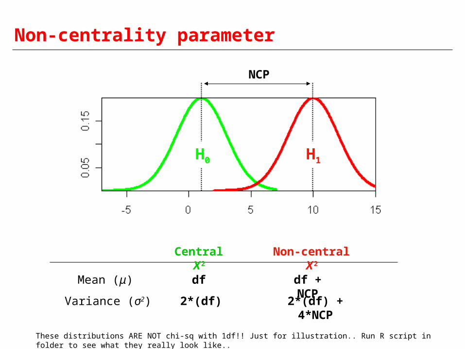
Non-centrality parameter

H0 H1

NCP

Mean (μ)

Variance (σ2)

Central Χ2

df

2*(df)

Non-central Χ2

df + NCP

2*(df) + 4*NCP

These distributions ARE NOT chi-sq with 1df!! Just for illustration.. Run R script in folder to see what they really look like..

H0 H1

NCP

Small NCP Big overlap between H0 and H1 distributions

Lower power

Large NCP Small overlap between H0 and H1 distributions

Greater power

Short practical on GPCGenetic Power Calculator is an online resource for carrying out basic power calculations.

For our 1st example we will use the probability function calculator to play with power

http://pngu.mgh.harvard.edu/~purcell/gpc/

1. Go to: ‘http://pngu.mgh.harvard.edu/~purcell/gpc/’Click the ‘Probability Function Calculator’ tab.

2. We’ll focus on the first 3 input lines. These refer to the chi-sq distribution that we’re interested in right now.

Using the Probability Function Calculator of the GPC

NCP

Degrees of freedom

of your test. E.g. 1df for univariate linkage (ignoring for now that it’s a mixture distribution)

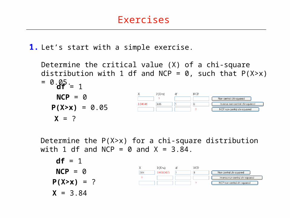
http://pngu.mgh.harvard.edu/~purcell/gpc/pdf.html

1. Let’s start with a simple exercise.

Determine the critical value (X) of a chi-square distribution with 1 df and NCP = 0, such that P(X>x) = 0.05.

Exercises

df = 1

NCP = 0

P(X>x) = 0.05

X = ?

Determine the P(X>x) for a chi-square distribution with 1 df and NCP = 0 and X = 3.84.

df = 1

NCP = 0

P(X>x) = ?

X = 3.84

2. Find the power when the NCP of the test is 5, degrees of freedom=1, and the critical X is 3.84.

Exercises

df = 1

NCP = 5

P(X>x) = ?

X = 3.84

What if the NCP = 10?

df = 1

NCP = 10

P(X>x) = ?

X = 3.84

NCP

3.84

NCP = 5

NCP = 10

3.84

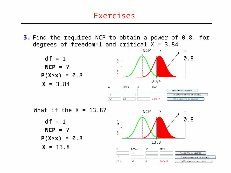
3. Find the required NCP to obtain a power of 0.8, for degrees of freedom=1 and critical X = 3.84.

Exercises

df = 1

NCP = ?

P(X>x) = 0.8

X = 3.84

What if the X = 13.8?

df = 1

NCP = ?

P(X>x) = 0.8

X = 13.8

NCP

3.84

NCP = ? = 0.8

NCP

13.8

NCP = ? = 0.8

2. Estimate power for linkage

and association

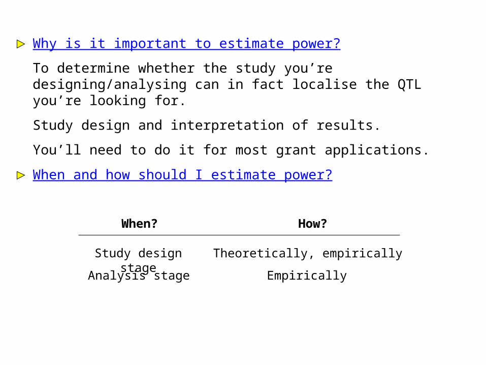
Why is it important to estimate power?

To determine whether the study you’re designing/analysing can in fact localise the QTL you’re looking for.

Study design and interpretation of results.

You’ll need to do it for most grant applications.

When and how should I estimate power?

Study design stage

Analysis stage

How?

Theoretically, empirically

Empirically

When?

Theoretical power estimation

NCP determines the power to detect linkage

NCP = μ(H1 is true) - df

H0 H1

NCP

If we can predict what the NCP of the test will be, we can estimate the power of the test

4. Marker informativeness (i.e. Var(π) and Var(z))


*Linkage*Variance Components linkage analysis (and some HE extensions)

zCovVVzVarVVarVr

rssNCP DADA ,ˆˆ

1

1

2

1 2222

2

1. The number of sibs in the sibship (s)

2. Residual sib correlation (r)

3. Squared variance due to the additive QTL component

(VA)

5. Squared variance due to the dominance QTL

component (VD).

^

Sham et al. 2000 AJHG 66: 1616

Another short practical on GPC

The idea is to see how genetic parameters and the study design influence the NCP – and so the power – of linkage analysis

1. Go to: ‘http://pngu.mgh.harvard.edu/~purcell/gpc/’Click the ‘VC QTL linkage for sibships’ tab.

Using the ‘VC QTL linkage for sibships’ of the GPC

http://pngu.mgh.harvard.edu/~purcell/gpc/qtllink.html

http://pngu.mgh.harvard.edu/~purcell/gpc/qtllink.html

1. Let’s estimate the power of linkage for the following parameters:

Exercises

QTL additive variance: 0.2

QTL dominance variance: 0

Residual shared variance: 0.4

Residual nonshared variance: 0.4

Recombination fraction: 0

Sample Size: 200

Sibship Size: 2

User-defined type I error rate: 0.05

User-defined power: determine N : 0.8

Power = 0.36 (alpha = 0.05)Sample size for 80% power = 681 families

2. We can now assess the impact of varying the QTL heritability

Exercises






Sample Size: 200

Sibship Size: 2




3. … the sibship size

Exercises






Sample Size: 200

Sibship Size: 3




CaTS performs power calculations for large genetic association studies, including two stage studies.

http://www.sph.umich.edu/csg/abecasis/CaTS/index.html

Theoretical power estimation *Association:

case-control*

TDT Power calculator, while accounting for the effects of untested loci and shared environmental factors that also contribute to disease risk

http://pngu.mgh.harvard.edu/~mferreira/power_tdt/calculator.html


*Association: TDT*


Advantages: Fast, GPC, CaTS

Disadvantages: Approximation, may not fit well

individual study designs, particularly if one needs to

consider more complex pedigrees, missing data,

ascertainment strategies, different tests, etc…

Empirical power estimation

Mx: simulate covariance matrices for 3 groups (IBD 0, 1 and 2 pairs) according to an FQE model (i.e. with VQ > 0) and then fit the wrong model (FE). The resulting test statistic (minus 1df) corresponds to the NCP of the test.

See powerFEQ.mx script.

Still has many of the disadvantages of the theoretical approach, but is a useful framework for general power estimations.

Simulate data: generate a dataset with a simulated marker that explains a proportion of the phenotypic variance. Test the marker for linkage with the phenotype. Repeat this N times. For a given α, Power = proportion of replicates with a P-value < α (e.g. < 0.05).

http://pngu.mgh.harvard.edu/~mferreira/

Empirical power estimation *Linkage /

Association*

Example with LINX

3. How to improve power

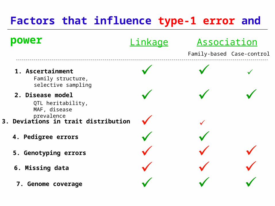
Factors that influence type-1 error and

power

1. Ascertainment

2. Disease modelQTL heritability, MAF, disease prevalence

Family structure, selective sampling

3. Deviations in trait distribution

4. Pedigree errors

5. Genotyping errors

7. Genome coverage

Linkage Association Family-based Case-control

6. Missing data

Pedigree errors

Definition. When the self-reported familial relationship for a given pair of individuals differs from the real relationship (determined from genotyping data). Similar for gender mix-ups.

Impact on linkage and FB association analysis. Increase type-1 error rate (can also decrease power)

Detection. Can be detected using genome-wide patterns of allele sharing. Some errors are easy to detect. Software: GRR.

Correction. If problem cannot be resolved, delete problematic individuals (family)

Boehnke and Cox (1997), AJHG 61:423-429; Broman and Weber (1998), AJHG 63:1563-4; McPeek and Sun (2000), AJHG 66:1076-94; Epstein et al. (2000), AJHG 67:1219-31.

Pedigree errors *Impact on

linkage*

• CSGA (1997) A genome-wide search for asthma susceptibility loci in ethnically diverse populations. Nat Genet 15:389-92

• ~15 families with wrong relationships

• No significant evidence for linkage

• Error checking is essential!

http://www.sph.umich.edu/csg/abecasisGRR

Pedigree errors

*Detection/Correction*

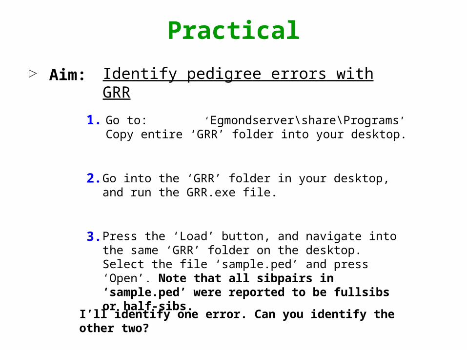
Practical

Aim:

Identify pedigree errors with GRR

1. Go to: ‘Egmondserver\share\Programs’Copy entire ‘GRR’ folder into your desktop.

2. Go into the ‘GRR’ folder in your desktop, and run the GRR.exe file.

3. Press the ‘Load’ button, and navigate into the same ‘GRR’ folder on the desktop. Select the file ‘sample.ped’ and press ‘Open’. Note that all sibpairs in ‘sample.ped’ were reported to be fullsibs or half-sibs.

I’ll identify one error. Can you identify the other two?

Summmary


2. Estimate the power of linkage analysis

3. Improve the power of linkage analysis

Documents

Statistical Power Calculations