Power Calculations for Matched Case-Control Studies

William D. Dupont

Biometrics, Vol. 44, No. 4. (Dec., 1988), pp. 1157-1168.

Stable URL:

http://links.jstor.org/sici?sici=0006-341X%28198812%2944%3A4%3C1157%3APCFMCS%3E2.0.CO%3B2-9

Biometrics is currently published by International Biometric Society.

Your use of the JSTOR archive indicates your acceptance of JSTOR's Terms and Conditions of Use, available athttp://www.jstor.org/about/terms.html. JSTOR's Terms and Conditions of Use provides, in part, that unless you have obtainedprior permission, you may not download an entire issue of a journal or multiple copies of articles, and you may use content inthe JSTOR archive only for your personal, non-commercial use.

Please contact the publisher regarding any further use of this work. Publisher contact information may be obtained athttp://www.jstor.org/journals/ibs.html.

Each copy of any part of a JSTOR transmission must contain the same copyright notice that appears on the screen or printedpage of such transmission.

The JSTOR Archive is a trusted digital repository providing for long-term preservation and access to leading academicjournals and scholarly literature from around the world. The Archive is supported by libraries, scholarly societies, publishers,and foundations. It is an initiative of JSTOR, a not-for-profit organization with a mission to help the scholarly community takeadvantage of advances in technology. For more information regarding JSTOR, please contact support@jstor.org.

http://www.jstor.orgWed Mar 26 16:32:58 2008

BIOMETRICS44, 1 157- 1 168 December 1988

Power Calculations for Matched Case-Control Studies

William D. Dupont

Division of Biostatistics, Department of Preventive Medicine, Vanderbilt University School of Medicine, Nashville, Tennessee 37232, U.S.A.

Power calculations are derived for matched case-control studies in terms of the probability po of exposure among the control patients, the correlation coefficient 4 for exposure between matched case and control patients, and the odds ratio $ for exposure in case and control patients. For given Type I and Type I1 error probabilities cr and /3, the odds ratio that can be detected with a given sample size is derived as well as the sample size needed to detect a specified value of the odds ratio. Graphs are presented for paired designs that show the relationship between sample size and power for a = .05, (I= .2, and different values of p,, 4, and $. The sample size needed for designs involving M matched control patients can be derived from these graphs by means of a simple equation.

These results quantify the loss of power associated with increasing correlation between the exposure status of matched case and control patients. Sample size requirements are also greatly increased for values of p, near 0 or 1. The relationship between sample size, $, 4, and p, is discussed and illustrated by examples.

1. Introduction

This paper presents a new series of isographs for power calculations and sample size estimation from matched 2 x M case-control studies. The question of sample size determination in matched 2 X 2 tables has been considered by Schlesselman (1982) and more recently by Parker and Bregman (1986) and Connett, Smith, and McHugh (1987). All of these authors express their sample size calculations in terms of the true odds ratio that is to be detected with a given power and Type I error probability level. Schlesselman estimates the number of discordant case-control pairs and then assumes independence in the exposure probabilities for cases and controls to obtain total sample size estimates. Connett et al. (1987) use an unconditional approach that requires an estimate of the probability that a case-control pair will have an unexposed case patient and an exposed control patient. When such an estimate is unavailable, they also assume independence in the exposure probabilities of cases and controls. This assumption is unrealistic because in most matched studies, exposure in a case patient is correlated with exposure in his matched control. Also, estimating the probability of a discordant pair can be very difficult in the absence of pilot data. Parker and Bregman (1986) avoid the independence assumption by permitting the user to specify a heterogeneous exposure distribution in different subgroups of the control population. Although this approach is a great improvement over previous methods, it is sometimes difficult to make plausible estimates of this exposure distribution. Parker and Bregman also assume that the disease incidence in unexposed patients does not vary with different values of the matching variables. This assumption is often unrealistic. For example, in an age-matched study of smoking and lung cancer it would imply that lung cancer incidence among nonsmokers does not increase with age.

Key words: Case-control studies; Matching; Sample size estimation; Power calculations.

1157

1158 Biometries, December 1988

Miettinen (1968), Duffy (1984), and Connor (1987) have also considered the problem of power calculations for matched tables. In these papers the alternative hypothesis is expressed in terms of the difference between the probabilities of obtaining the two different types of discordant case-control pairs. For epidemiologic studies it is perhaps more useful to express power calculations in terms of odds ratios.

This paper gives the derivation of the odds ratio that can be detected with power 1 - 0 given a two-sided Type I error probability a , N case patients, M matched control patients per case, the probability of exposure po among control patients, and the correlation coefficient 4 for exposure in matched pairs of case-control patients. The corresponding number of case patients needed to detect a given odds ratio $ with power 1 - and Type I error probability a is also derived. A major advantage of this approach is that power calculations are expressed directly in terms of the correlation coefficient for exposure between matched case and control subjects and the prevalence of exposure in the control group. This facilitates the drawing of isographs, which greatly simplify the task of sample size estimation in matched case-control studies, and which permit epidemiologists to gain an insight into the relationship between power, sample size, and these other variables.

2. Notation and Assumptions

Consider a population of case patients with some disease and control patients who do not have this illness. Some of these patients have had prior exposure to a risk factor of interest, and all subjects can be classified by different levels of a variable that confounds the association between the risk factor and the disease. We wish to estimate the odds ratio $ of developing the disease in exposed and unexposed patients who have equal values of the confounding variable (see Breslow and Day, 1980). To do this we first select a random sample of N case patients. We then stratify the population by the confounding variable and assume that $ is constant across all strata. For each selected case patient we randomly sample M matched control patients from the same stratum as the corresponding case patient. Let xk= 1 or 0 if the kth sampled case patient was or was not exposed, respectively, and let y,, = 1 or 0 denote the corresponding exposure status of the first matched control for this patient. Let p,, denote the probability that xk = i and yk = j. Let po = p l , + pol denote the probability that a sampled control patient is exposed. Let p l = p, , + plo denote the probability that a sampled case patient is exposed and let go = 1 - po and q, = 1 - p , . Let 4 denote the phi coefficient between x k and yk. (It is easily shown that 4 is algebraically identical to the Pearson product-moment correlation coefficient p between xkand yk.) Let a and p denote the Type I and Type I1 error probabilities, respectively. In the remainder of this paper the terms case and control patient refer to sampled subjects as opposed to members of the target population.

For any given values of a , 0, $, 4, and po, the value of N needed to detect $ with power 1 - 0 can be decreased by increasing M. Suppose NI and NM denote the number of case patients needed to attain the required power given 1 and M matched controls, respectively. Let E,w = NM/NI denote the reduction in N relative to a paired design that can be obtained by selecting M controls per case.

3. Derivation of Results

By definition 4 = cov(xk, yk)/(a,a,):It can be easily shown that

1160 Biometries, December 1988

It follows that

Substituting the preceding expressions into equation (7)permits us to write N as a function of po, 4, I), a, and P. Thus, equation (7)can be used to determine the number of case patients needed to detect iC/ with power 1 - /3 given a, pO, 4, and M.

F,w = NjW/NIcan also be calculated from equation (7)by taking the ratio of sample sizes needed using 1 and M controls per case, respectively. The dots in Figure 1 show values of FM plotted as a function of po for a = .05, /3 = .2, iC/ = 6, 4 = . I , and M = 2, 3 , 4, 8, and 16. This figure is typical of similar figures for a wide range of values of a, /3, I), 4, and M. For given values of a, /3, iC/, and 4, these figures indicate that F, can be closely approximated by linear functions jlbf(pO)that have a common intersection point on the line FI = 1 and for which FjbI(c)= (M + 1)/(2M)for some positive c. This latter condition can be met by setting k,f(pO)( M + 1)/(2M)+ bxt(pO c).The common intersection of these curves = -at some point pO= k + c implies that 1 = (M + 1)/(2M)+ bjVfk,giving

M + 1 ( M - 1 ) ~ M C , ) = +

2Mk (PO- c),

where k and c are both functions of a, P, 4, and iC / . The accuracy and utility of this expression are discussed in the next section. The straight lines drawn on Figure 1 give &,(PO) for M = 2, 3 , 4, 8 , and 16. The accuracy of kWas an estimate of EWis remarkable.

Figure 1. This figure shows F,\,, the reduction in N relative to a paired design that can be obtained by selecting M controls per case. The dots show the true values of F , for 1M = 2, 3, 4, 8, and 16. The straight lines show the estimated value of F,, using equation (8) with c = .573 and k = 1.620. In this

example, 4 = .1, = 6.0, cu = .05, and f i = .2.

1161 Power Calculations for Matched Case-Control Studies

4. Using the Isographs

Figures 2-7 present sample size isographs for paired case-control studies that were derived using equation (7). The value of 4 is constant in each graph and equals 0, . l , .2, .3, .4, and .5 in Figures 2 through 7, respectively. The values of a and 0equal .05 and .2, respectively, in all graphs and test the null hypothesis that $ = 1 against a two-sided alternative hypothesis. The abscissa of each graph is po while the ordinate is the value of $ that can be detected with 80% power. Each figure shows isographs of constant case sample size N as a function of po and $. By interpolating between these lines the reader can either determine the value of $ that can be detected with a given sample size or the sample size required to detect a given value of $.

The value of $ in Figures 2-7 ranges from 1 through 6. However, these graphs can also be used for studies of factors that are thought to reduce disease risk. For example, if factor X reduces disease risk with odds ratio $ < 1, then the absence of X increases the disease risk with odds ratio l/$ > 1. Thus, sample size calculations using these figures can be based on the risk associated with not having factor X.

For the values of 4 and $ described in Figures 2-7, it can be shown empirically that FjWcan be closely approximated by equation (8). The values of k and c needed in equation (8) are given in Table 1. Equation (8) and Table 1 can be used in combination with Figures 2-7 to determine the sample size needed to detect a given value of $ using more than one

Figure 2. The numbers on the lines on this graph indicate constant sample sizes for paired case- control studies. Each line shows the value of the odds ratio $ that can be detected with 80% power as a function of exposure prevalence p, for control subjects. These curves are derived assuming a two- sided Type I error probability of a = .05 and a correlation coefficient for exposure between matched

subjects of 4 = 0.

O .YJ z .+ fl "52 '3w c d

3

00 ZB ' " -a0 3

2 '2 + wG ' G 0 ,

0 2 0 o o c

Q 2.2 .k cd

. g-g 0 g 8

w w .2 75

t'! :'Gi 0 Er,

E, .e" h + -

? S E 0 * m

E 2 s

. ~ . l

1163Power Calculations for Matched Case-Control Studies

&=0.05 ,B=0.2 p=0.31 . 0 n m 7 - r 1 r r r r r m ~ 1 1 1 u r 0 I 1 s 0 ~ ~ 1 1 1 ~ 1 r 0 ~ r r 1

0 . 0 0 . 2 0 . 4 0 . 6 0 . 8 1 . 0

p 0 Figure 5. Isographs of constant sample size for paired case-control studies. This figure differs from

Figure 2 only in that the correlation coefficient 4 equals .3.

$ a.0.05 /3=0.2 (p=0.41 . 0 , ! ~ , T ~ ~ . ~ - , . ~ - ~ ~ c ~ ~ . ~ ~ ! ~ ~ ~ ~ ~ n . [ ~ r ~ ~ ~ ~ ~ u T l . m u . ~ ~

0 . 0 0 . 2 0 . 4 0 . 6 Q . 8 1 . O

p0 Figure 6. Isographs of constant sample size for paired case-control studies. This figure differs from

Figure 2 only in that the correlation coefficient 4 equals .4.

Biometrics, December 1988

Figure 7. Isographs of constant sample size for paired case-control studies. This figure differs from Figure 2 only in that the correlation coefficient 4 equals .5.

matched control per case. For example, suppose po = .6, 4 = .2, and that we wish to detect $ = 3 with power .8. Then Figure 4 shows that we should select 80 case patients using a paired design. If we select 3 control patients per case, then Table 1 gives k = 3.669 and c = 1.028 when 4 = .2 and $ = 3. Substituting these values into equation ( 8 )with M = 3 and po = .6 gives k 3 ( . 6 )= .6278. Thus, with N = 80k3( .6)= 50 cases and 3 controls per case we can detect $ = 3 with 80% power. In this example the true value of F3 equals .6264, which also yields N = 50. Thus, in this example, the estimate of N obtained by using Table 1 is correct to the nearest integer. Table 2 shows the maximum percentage error in PJIffor values of M between 2 and 16 and the values of po, 4, and $ given in the figures. For 2, 3 , or 4 controls per case, the error in is always less than 3%. Larger values of M are associated with higher errors when po is small. In this case P,tf overestimates FIf and hence overestimates the required number of case patients.

Schlesselman (1982, p. 168) recommends multiplying the paired-case sample size by ( M + 1 ) / ( 2 M ) to obtain the equivalent case sample size with M matched controls per group. Equation ( 8 ) shows that this approach provides an acceptable approximation if po is near c or when k is large. From Table 1 we see that k increases as $ approaches 1 . Thus, Schlesselman's multiple control correction is asymptotically correct for large N since N approaches infinity as $ approaches 1 . Equation ( 8 ) shows, however, that Schlesselman's adjustment is inaccurate for many reasonable values of po and $. For small values of po this adjustment will greatly overestimate the number of case patients needed to achieve the required power.

Software is available from the author on request which derives the value of $ that can be detected with power 1 - P given a, 4, po, N, and M, as well as the case sample size N

1165 Power Calculations for Matched Case-Control Studies

Table 1 Coeflcients k and c for power calculations with multiple controls per case. These coe&ients are used

in equation (8) , with a = .05 and P = .2.

Correlation coefficient 4

Table 2 Maximum percentage error in efJiciency ratio p,L,,(p,)

l < $ s 3 3 < $ 6 6

needed to detect a true value of # with power 1 - 0given a, 0,po, and M. These programs calculate the exact power associated with M controls per case without using the approxi- mation of F , given in equation (8).

5. Comparison with Schlesselman's Method

Suppose 4 = .2 and po = .6. Figure 4 shows that # = 3 can be detected with 80% power when N = 80. Substituting these values of 4, PO, and # into equations (2)-(5)gives the following 2 x 2 table of exposure probabilities for a matched pair of case-control patients:

Case -+ Total

+ P I ]= .509 pol = .091 p, = .6 Control

- P I O= .272 poo = .I28 q, = .4

Total p,=.781 q l = . 2 1 9 1

[It is worth noting as a check on the validity of equations (2)-(5)that # = p,o/pol= 3.0 and that 4 = .20 using equation ( I ) . ] The probability of a discordant pair is thus p lo + pol = .363 and hence the expected number of discordant pairs given a sample size of N = 80 case patients equals 80 x .363 = 29.0. In comparison, equation (6.20) of Schlesselman

1166 Biometries, December 1988

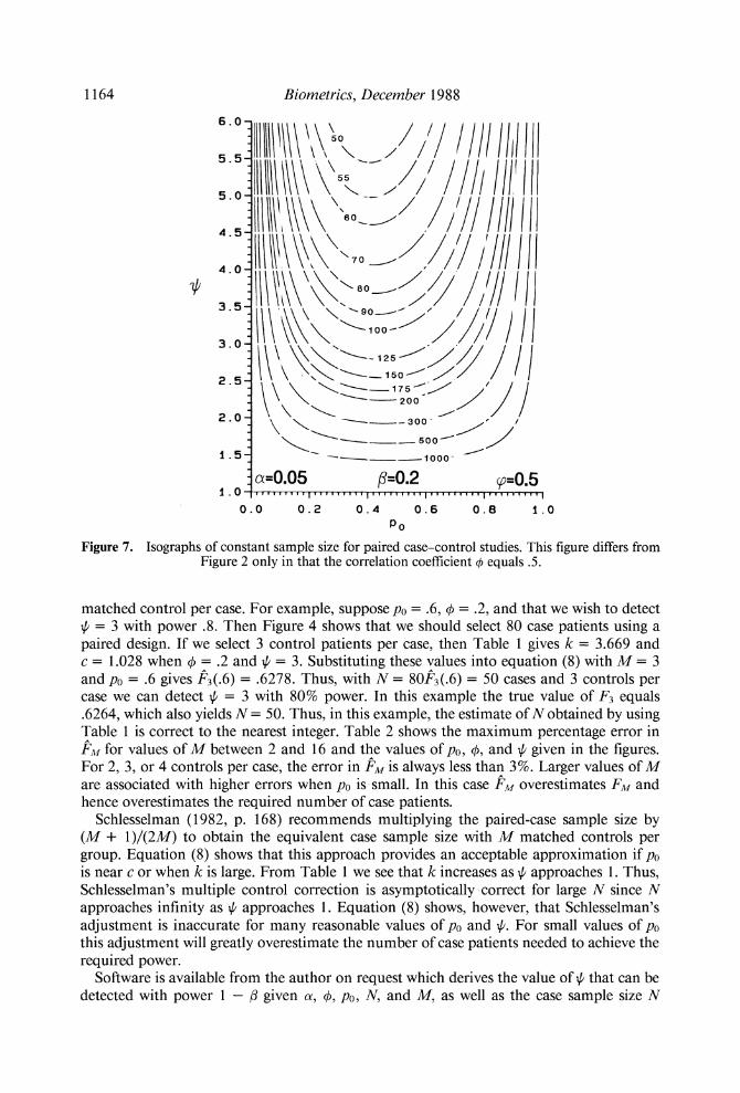
(1982)gives that the number of discordant pairs needed to detect $ = 3.0 with 80% power is

which is in close agreement with the expected number of discordant pairs given above. Thus, the method presented in this paper can be thought of as a generalization of Schlesselman's method to the case in which 6 # 0. Equation (6.23) of Schlesselman estimates N to be m / ( p o q l + p l q o ) = 65. This estimate, which is derived under the assumption that 6 = 0, overestimates the expected number of discordant pairs and hence underestimates the sample size needed for the required power.

6. Estimating po and 4

po is the probability that a sample control patient will be exposed. The control sample is not, however, a random sample from the control population but, rather, is matched to a random sample of case patients from the case population. Thus, an unbiased estimate of the exposure prevalence in the control population is not necessarily an unbiased estimate ofpo.Let po(c)denote the probability that a control subject with confounding variable c is exposed, Dc,,,(c) and Dctl(c)denote the probability density functions of c among the case and control populations, respectively, and let p,* denote the exposure prevalence in the control population. Then

w = Sw(c)Dcase(c) ( 9 )dc

while

When c is positively associated with both disease incidence and exposure prevalence, p,* will underestimate po. Note, however, that if po(c) is constant, then po = p,* and p,* will approximate po whenever the exposure prevalence in the control population does not vary greatly with c. In many case-control studies, there is little association between the confound- ing variable and the exposure variable in the control population. For such studies it is reasonable to estimate po by the exposure prevalence in the general population. When a more accurate estimate of po is required, it may be estimated through equation (9) .To do this it is necessary to obtain estimates of the confounder-specific exposure prevalence rates in the control population as well as estimates of the distribution of case patients with respect to c. [Note that the method of Parker and Bregman (1986)also requires estimates of the confounder-specific exposure prevalence rates and that they estimate the distribution of case patients with respect to c by assuming a constant disease incidence among unexposed subjects.]

The correlation coefficient 4 can be estimated from previous studies that publish matched 2 x 2 contingency tables using equation (5.2) of Fleiss (1981).Of course, such data could also be used to estimate the proportion of discordant pairs, which in turn could be used to obtain sample size estimates using Schlesselman's (1982)method. However, the proportion of discordant pairs is likely to vary considerably between different studies since it depends not only on 4 but also on the exposure prevalence po and the odds ratio $. In contrast, estimates of 6 should be more stable between similar studies. When no estimate of 6 is available, investigators may prefer to perform their power calculations under the assumption

1167 Power Calculations for Matched Case-Control Studies

that 6 equals, say, .2 rather than make the questionable independence assumption required by most other methods.

7. Conclusions

The graphs presented in this paper demonstrate and quantify the complex relationship between sample size, power, the magnitude of the control exposure prevalence po, and the exposure correlation coefficient 4. Figures 2-7 illustrate the substantial loss in power that occurs with increasing correlation between the exposure status of matched case-control pairs. For example, when 6 = 0, the minimum value of + that can be detected with 80% power and N = 50 is 3.14. This minimum value increases steadily with increasing 6, reaching 5.45 when 6 = .5. The value of po has little effect on power when + is low and po is not too extreme (say + < 2 and .2 < po S .8). However, the precise value of po has a critical effect on the power when po is near 0 or 1, or when the sample size is small. This result is due to the influence of po and + on the expected number of discordant case- control pairs. The method presented here will provide accurate power calculations whenever reasonable estimates of po and 6 are available. Even when no appropriate estimates of 6 can be found, investigators can still avoid the independence assumption for exposure among matched subjects by selecting a reasonable value of 4. This will produce sample size estimates that are more conservative and plausible than those based on the indepen- dence assumption.

I would like to thank W. Dale Plummer, Jr. for writing the software for this paper and Shirley Carson and Becky Wieland for assistance in preparing the manuscript. This research was supported by research grants and contracts from the Department of Health and Human Services #HL- 14 192, NO 1-AI-52593, 5P30NIADK26657, R0 1-CA405 17, and RO 1-CA46492.

La puissance des itudes cas-tkmoins apparikes est diterminie en fonction de po, probabilitk d'expo- sition chez les timoins, 4, coefficient de corrilation entre les expositions chez les malades et tkmoins appariks, et $, "odds-ratio" mesurant la relation exposition-maladie. Pour des risques de premiire et seconde espice donnks, cu et p, l'odds-ratio qui peut itre dktectk est calculk en fonction de la taille de l'kchantillon et inversement. On prksente des abaques qui, pour les ktudes 1- 1, montrent la relation entre la taille de l'kchantillon et la puissance pour cu = .05, P = .2 et diffkrentes valeurs de po, 4, et +. Le passage aux itudes 1-M se fait au moyen d'une iquation simple.

Ces rksultats quantifient la perte de puissance associie a une augmentation du coefficient de corrklation 4. Des valeurs de po voisines de 0 au 1 nkcessitent des effectifs importants. Des exemples illustrent ces rksultats.

Breslow, N. E. and Day, N. E. (1980). Statistical Methods in Cancer Research: Volume I . The Analysis of Case-Control Studies. Lyon: International Agency for Research on Cancer.

Connett, J. E., Smith, J. A., and McHugh, R. B. (1987). Sample size and power for pair-matched case-control studies. Statistics in Medicine 6 , 53-59.

Connor, R. J. (1 987). Sample size for testing differences in proportions for the paired-sample design. Biometries 43, 207-2 1 1.

Duffy, S. W. (1984). Asymptotic and exact power for the McNemar test and its analogue with R controls per case. Biornetrics 40, 1005- 10 15.

Fleiss, J. L. (1981). Statistical Methods for Rates and Proportions, 2nd edition. New York: Wiley. Miettinen, 0 . S. (1968). On the matched-pairs design in the case of all-or-none responses. Biornetrics

24. 339-352.

1168 Biometries, December 1988

Parker, R. A. and Bregman, D. J. (1986). Sample size for individually matched case-control studies. Biometries 42, 9 19-926.

Schlesselman, J. J. (1982). Case-Control Studies: Design, Conduct, Analysis. New York: Oxford University Press.

Received June 1987; revised April 1988.

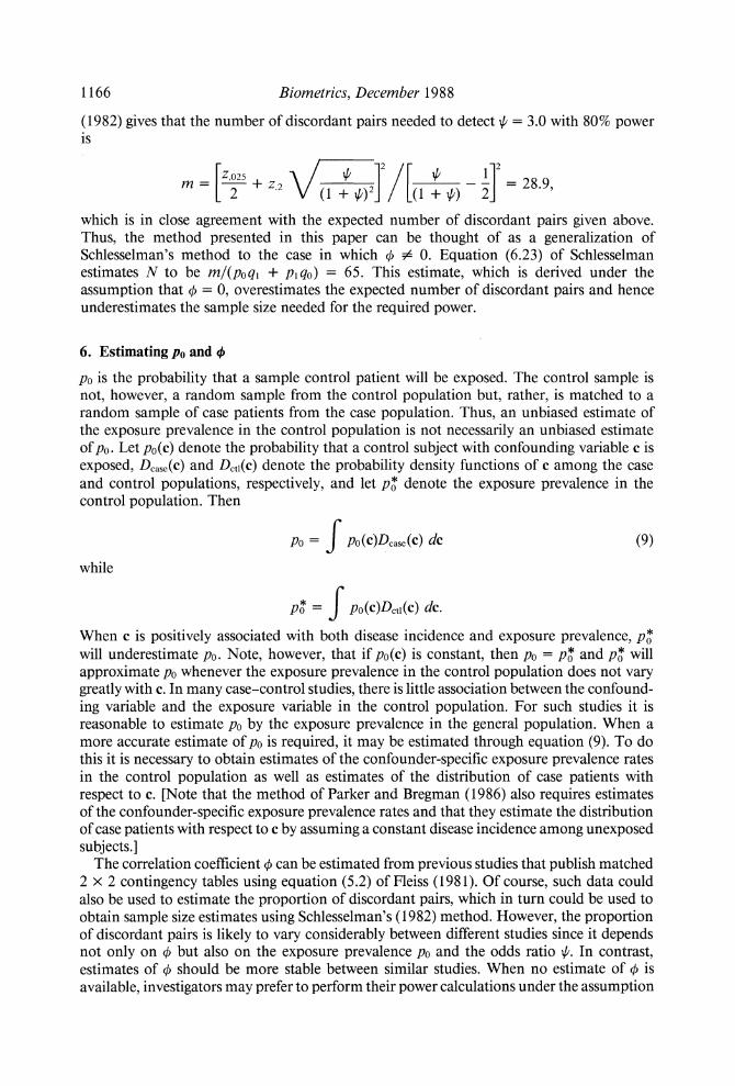
We wish to express pl in terms of $, po, and 4 . It follows from the definition of the terms p,, that $ = P I O ~ P O , , PO = P I O- POI= ($ - l)po1,PI^ = P O - p o l , and poo = q1-P I - p o l .Hence, pol =

( P I - PO)/($ - 11, P I O= $ ( P I - PO)/($ - 1 1 , P I I= ($PO - p I ) l ( $ - I ) , and poo = ($ql - go)/($ - I ) .When $ Z 1 we can substitute these expressions into equation ( 1 ) to obtain

Equation (10)can be rewritten in the form

where A and B are functions of $ and pa. Squaring equation ( 1 1 ) yields

(B' + 4 " ~ :+ ( 2 A B - #J2)pl+ A' = 0 , ( 1 2 )

which is a quadratic equation in p , . Equation (12)has two roots:

which is also the solution to equation ( 1 I ) , and another root that solves -4 = ( A + B P ~ ) / ~ . Thus, to prove that equation ( 1 3 ) is the solution to equation ( 1 1 ) it is sufficient to substitute (13)into the right-hand side of ( 1 1 ) and then show that this expression has the same sign as 4. This is a straightforward exercise. It is interesting to note that when $ = 1 , pl = po. Hence, equation (13) is correct for all positive values of $. Note also that when #J = 0 , (13) reduces to (6.2) in Schlesselman ( 1 982).

You have printed the following article:

Power Calculations for Matched Case-Control StudiesWilliam D. DupontBiometrics, Vol. 44, No. 4. (Dec., 1988), pp. 1157-1168.Stable URL:

http://links.jstor.org/sici?sici=0006-341X%28198812%2944%3A4%3C1157%3APCFMCS%3E2.0.CO%3B2-9

This article references the following linked citations. If you are trying to access articles from anoff-campus location, you may be required to first logon via your library web site to access JSTOR. Pleasevisit your library's website or contact a librarian to learn about options for remote access to JSTOR.

References

Sample Size for Testing Differences in Proportions for the Paired-Sample DesignRobert J. ConnorBiometrics, Vol. 43, No. 1. (Mar., 1987), pp. 207-211.Stable URL:

http://links.jstor.org/sici?sici=0006-341X%28198703%2943%3A1%3C207%3ASSFTDI%3E2.0.CO%3B2-Y

Asymptotic and Exact Power for the McNemar Test and Its Analogue with R Controls PerCaseStephen W. DuffyBiometrics, Vol. 40, No. 4. (Dec., 1984), pp. 1005-1015.Stable URL:

http://links.jstor.org/sici?sici=0006-341X%28198412%2940%3A4%3C1005%3AAAEPFT%3E2.0.CO%3B2-D

The Matched Pairs Design in the Case of All-or-None ResponsesOlli S. MiettinenBiometrics, Vol. 24, No. 2. (Jun., 1968), pp. 339-352.Stable URL:

http://links.jstor.org/sici?sici=0006-341X%28196806%2924%3A2%3C339%3ATMPDIT%3E2.0.CO%3B2-X

Sample Size for Individually Matched Case-Control StudiesR. A. Parker; D. J. BregmanBiometrics, Vol. 42, No. 4. (Dec., 1986), pp. 919-926.Stable URL:

http://links.jstor.org/sici?sici=0006-341X%28198612%2942%3A4%3C919%3ASSFIMC%3E2.0.CO%3B2-U

http://www.jstor.org

LINKED CITATIONS- Page 1 of 1 -