Statistical Modeling for Radiation Hardness Assurance … · Statistical Modeling for Radiation Hardness Assurance ... 0.030 0.035 0.040 ... Statistical Modeling for Radiation Hardness

Statistical Modeling for Radiation Hardness Assurance

Ray Ladbury Radiation Effects and Analysis Group NASA Goddard Space Flight Center

Presented by Ray Ladbury at the Hardened Electronics and Radiation Technology (HEART) 2014 Conference, Huntsville, AL, March 17-21, 2014 and published on radhome.gsfs.nasa.gov. 1

https://ntrs.nasa.gov/search.jsp?R=20140008964 2018-07-13T21:44:01+00:00Z

Presented by Ray Ladbury at the Hardened Electronics and Radiation Technology (HEART) 2014 Conference, Huntsville, AL, March 17-21, 2014 and published on radhome.gsfs.nasa.gov.

List of Abbreviations BJT—Bipolar Junction Transistor CL—Confidence Level DSEE—Destructive SEE JFET—Junction Field Effect Transistor MOSFET—Metal-Oxide-Semiconductor Field Effect Transistor RLAT—Radiation Lot Acceptance Test SEB—Single-Event Burnout SEE—Single-Event Effect SEGR—Single-Event Gate Rupture SEL—Single-Event Latchup SOI—Silicon on Insulator TID—Total Ionizing Dose RPP—Rectangular Parallelepiped WC—Worst Case

2


Outline I. Current RHA and It’s Statistical Models II. Other Sources of Data and How They Are Used III. Bayesian Probability and Why It’s Well Suited to RHA IV. Example: Bayesian SEE V. A More Complicated Example: Bayesian TID VI. Flight Heritage as data VII. Fitting data and Bounding rates in SEE VIII. Using Statistical Modelling to Meet Challenges of Destructive SEE IX. Conclusions

3

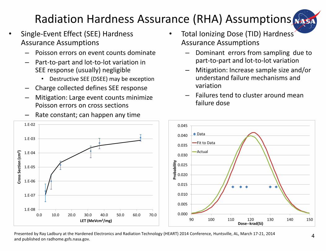
Radiation Hardness Assurance (RHA) Assumptions • Single-Event Effect (SEE) Hardness

Assurance Assumptions – Poisson errors on event counts dominate – Part-to-part and lot-to-lot variation in

SEE response (usually) negligible • Destructive SEE (DSEE) may be exception

– Charge collected defines SEE response – Mitigation: Large event counts minimize

Poisson errors on cross sections – Rate constant; can happen any time

• Total Ionizing Dose (TID) Hardness Assurance Assumptions

– Dominant errors from sampling due to part-to-part and lot-to-lot variation

– Mitigation: Increase sample size and/or understand failure mechanisms and variation

– Failures tend to cluster around mean failure dose

1.E-08

1.E-07

1.E-06

1.E-05

1.E-04

1.E-03

1.E-02

0.0 10.0 20.0 30.0 40.0 50.0 60.0 70.0

Cros

s Sec

tion

(cm

2 )

LET (MeVcm2/mg)

0.000

0.005

0.010

0.015

0.020

0.025

0.030

0.035

0.040

0.045

90 100 110 120 130 140 150

Prob

abili

ty

Dose--krad(Si)

Data

Fit to Data

Actual


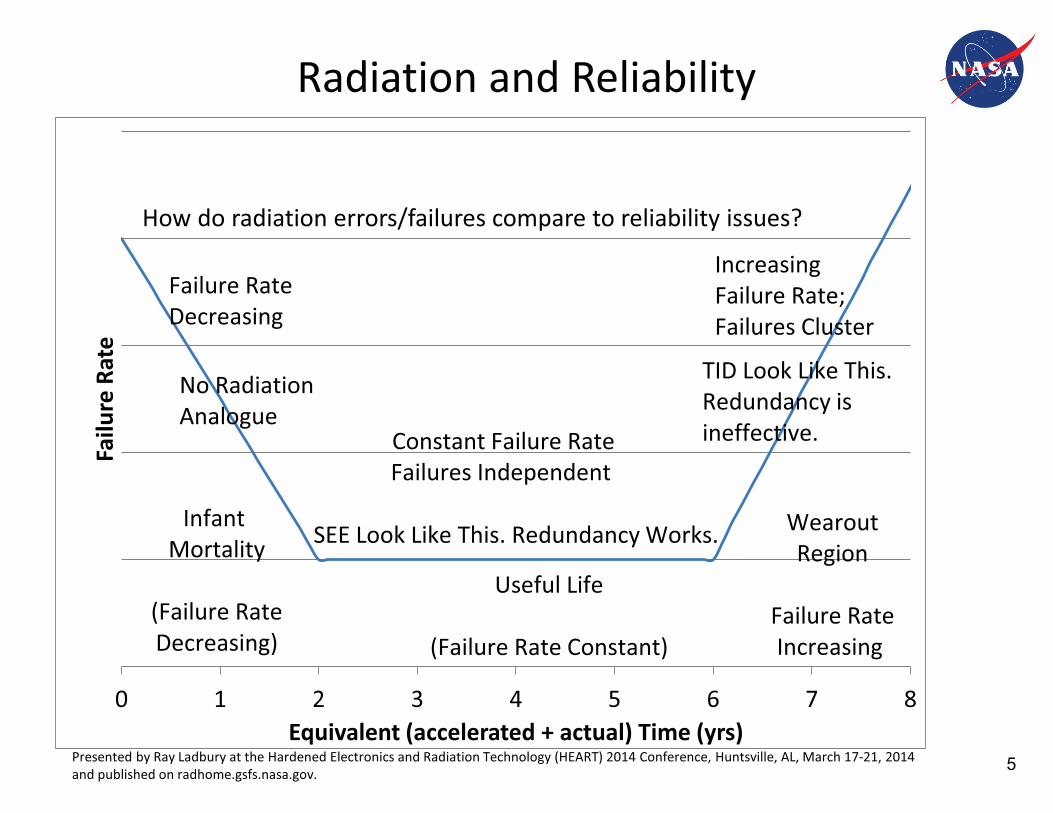
Radiation and Reliability

0 1 2 3 4 5 6 7 8

Failu

re R

ate

Equivalent (accelerated + actual) Time (yrs)

Infant Mortality

(Failure RateDecreasing)

Useful Life

(Failure Rate Constant)

WearoutRegion

Failure RateIncreasing

Failure Rate Decreasing

Constant Failure RateFailures Independent

Increasing Failure Rate;Failures Cluster

SEE Look Like This. Redundancy Works.

TID Look Like This. Redundancy is ineffective.

No Radiation Analogue

How do radiation errors/failures compare to reliability issues?


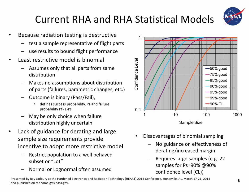
Current RHA and RHA Statistical Models • Because radiation testing is destructive

– test a sample representative of flight parts – use results to bound flight performance

• Least restrictive model is binomial – Assumes only that all parts from same

distribution – Makes no assumptions about distribution

of parts (failures, parametric changes, etc.) – Outcome is binary (Pass/Fail),

• defines success probability, Ps and failure probability Pf=1-Ps

– May be only choice when failure distribution highly uncertain

• Lack of guidance for derating and large sample size requirements provide incentive to adopt more restrictive model

– Restrict population to a well behaved subset or “Lot”

– Normal or Lognormal often assumed

• Disadvantages of binomial sampling – No guidance on effectiveness of

derating/increased margin – Requires large samples (e.g. 22

samples for Ps=90% @90% confidence level (CL))

0.1

1

1 10 100 1000

Con

fiden

ce L

evel

Sample Size

50% good75% good85% good90% good95% good99% good90% CL


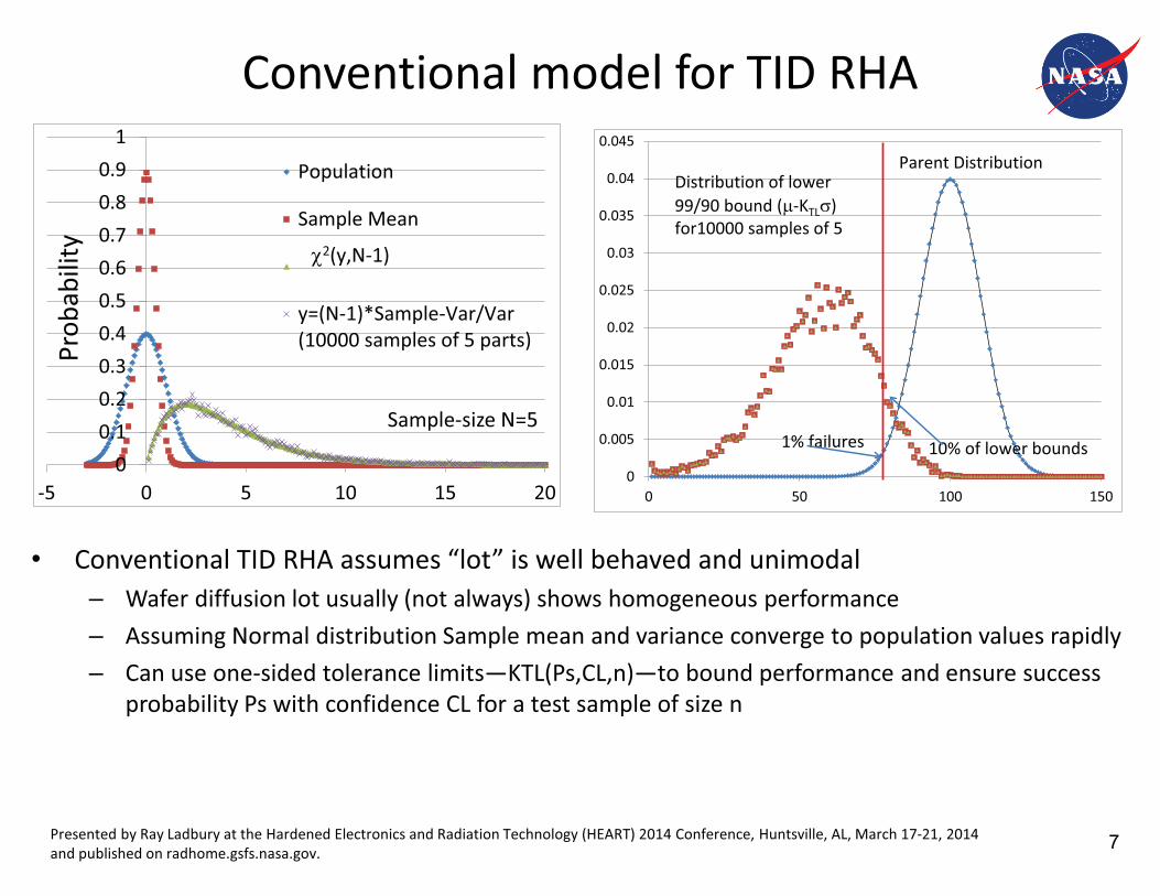
Conventional model for TID RHA

• Conventional TID RHA assumes “lot” is well behaved and unimodal – Wafer diffusion lot usually (not always) shows homogeneous performance – Assuming Normal distribution Sample mean and variance converge to population values rapidly – Can use one-sided tolerance limits—KTL(Ps,CL,n)—to bound performance and ensure success

probability Ps with confidence CL for a test sample of size n

0

0.005

0.01

0.015

0.02

0.025

0.03

0.035

0.04

0.045

0 50 100 150

Distribution of lower 99/90 bound (�-KTL�)for10000 samples of 5

Parent Distribution

1% failures 10% of lower bounds0

0.10.20.30.40.50.60.70.80.9

1

-5 0 5 10 15 20

Population

Sample Mean

y=(N-1)*Sample-Var/Var(10000 samples of 5 parts)

�2(y,N-1)

Sample-size N=5


Prob

abili

ty

7

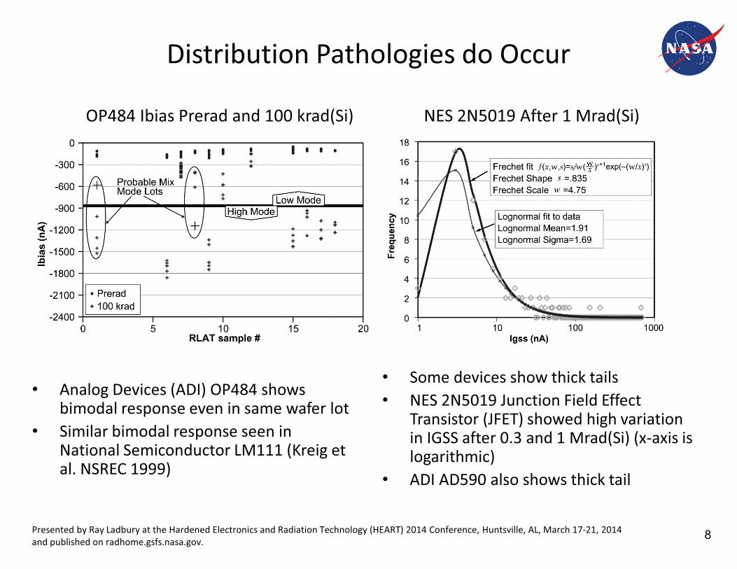
Distribution Pathologies do Occur

• Analog Devices (ADI) OP484 shows bimodal response even in same wafer lot

• Similar bimodal response seen in National Semiconductor LM111 (Kreig et al. NSREC 1999)

• Some devices show thick tails • NES 2N5019 Junction Field Effect

Transistor (JFET) showed high variation in IGSS after 0.3 and 1 Mrad(Si) (x-axis is logarithmic)

• ADI AD590 also shows thick tail

OP484 Ibias Prerad and 100 krad(Si) NES 2N5019 After 1 Mrad(Si)



When There’s No Lot-Specific Data

• Historical Data—Test data for the same part type/# as the flight parts, taken under similar application conditions

• Similarity/Process Data—Test data for parts with similar function fabricated at the same facility in the same process, taken under comparable application conditions

• Heritage Data—Data regarding past flight use of the same part type/#; heritage mission environments must usually be at least as severe as the current mission and application conditions must be comparable

• When you are really desperate – Physics—What do we know about the part and the radiation effects mechanisms that can

place limits on their severity—example: Silicon-on-Insulator (SOI) limits SEE susceptibility – Technology trends—How have the susceptibilities changed over previous “similar”

generations—e.g. SEL susceptibility for commercial SRAMs with minimum Complementary Metal Oxide Semiconductor (CMOS) feature size from 0.35 down to 0.11 microns

– Technology generation—Susceptibility and trends thereof for comparable technologies from the same and even other vendors

– Expert opinion—What do the smart kids think?

• None of these lines of evidence may restrict susceptibility in a meaningful way

9

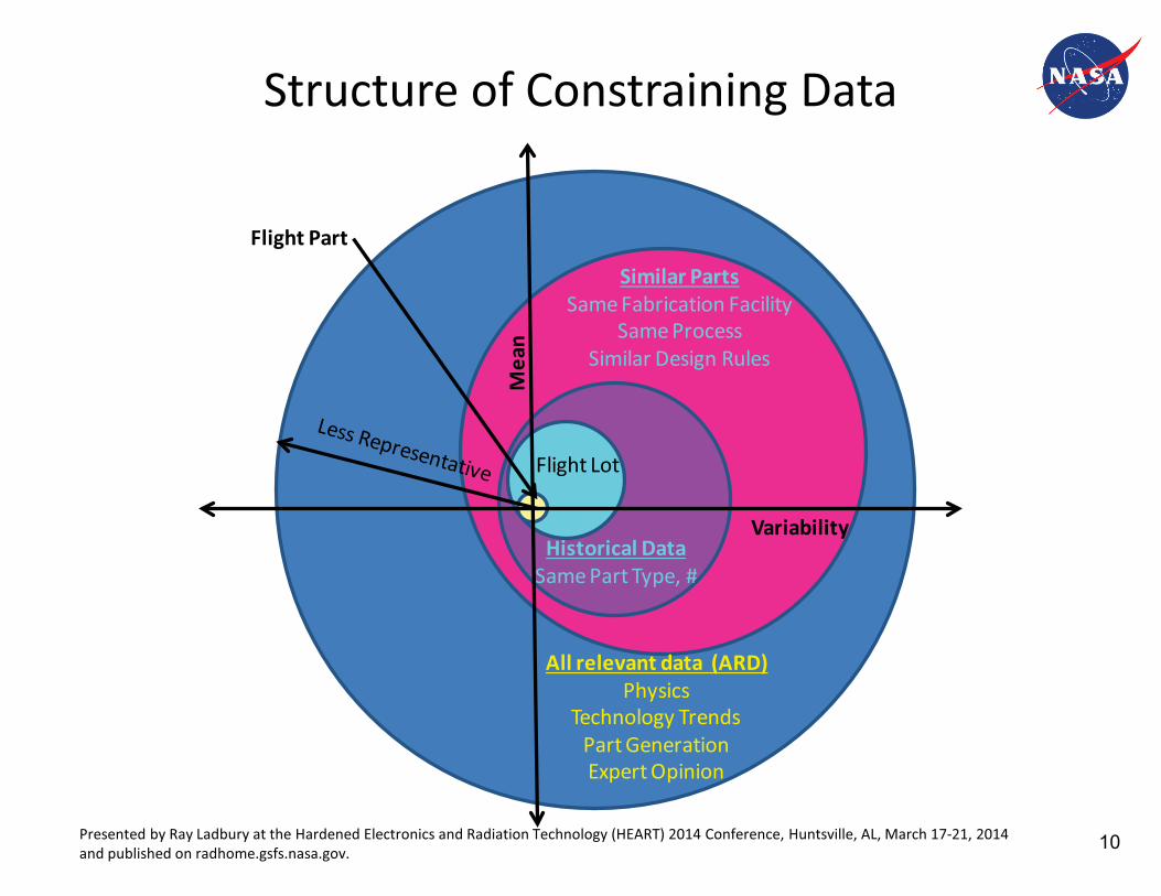
Structure of Constraining Data

All relevant data (ARD)Physics

Technology TrendsPart GenerationExpert Opinion

Similar PartsSame Fabrication Facility

Same ProcessSimilar Design Rules

Historical DataSame Part Type, #

Flight Lot

Flight Part

VariabilityM

ean


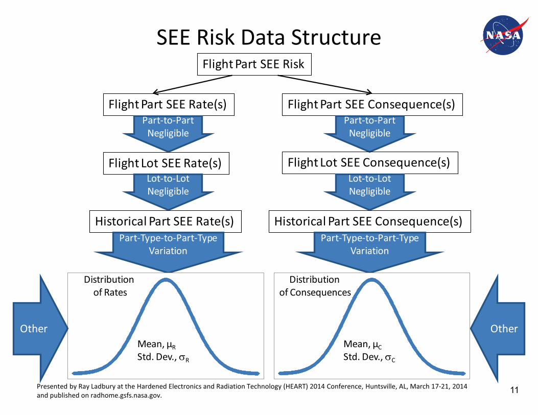
SEE Risk Data Structure

Flight Part SEE Rate(s) Flight Part SEE Consequence(s)Part-to-Part

NegligiblePart-to-Part

Negligible

Flight Lot SEE Rate(s) Flight Lot SEE Consequence(s)Lot-to-Lot Negligible

Lot-to-Lot Negligible

Historical Part SEE Rate(s) Historical Part SEE Consequence(s)Part-Type-to-Part-Type

Variation Part-Type-to-Part-Type

Variation

Flight Part SEE Risk

Distribution of Rates

Mean, μR

Std. Dev., �R

Distribution of Consequences

Mean, μC

Std. Dev., �C

Other Other


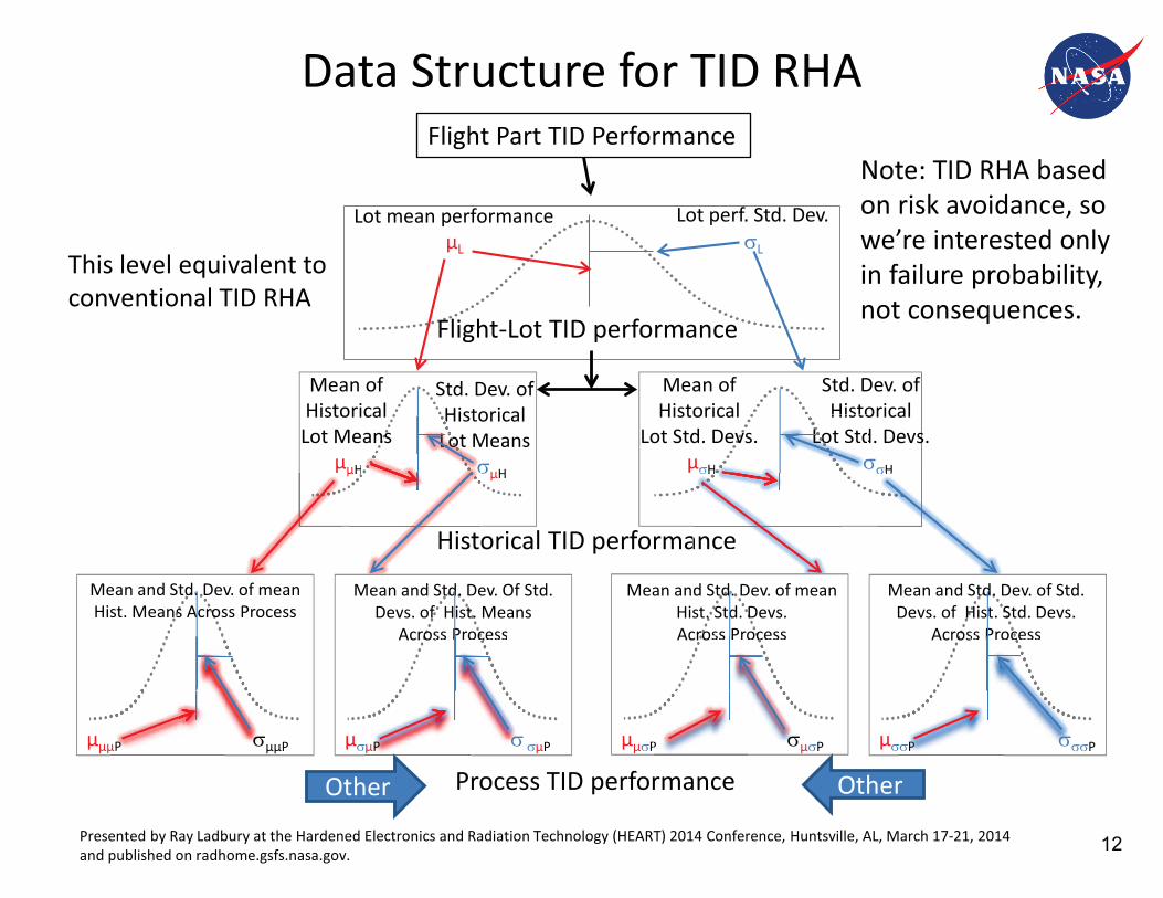
Data Structure for TID RHA


Flight Part TID Performance

Flight-Lot TID performance

Lot mean performanceμL

Lot perf. Std. Dev.�L

Historical TID performance

Mean ofHistoricalLot Means

μμH

Std. Dev. ofHistorical

Lot Means�μH

HistoLLLLLLLLLLLLLLLLLLLLLLLooooooooooooooooooott MoooooooLLLLL

�

Mean ofHistorical

Lot Std. Devs.μ�H

Std. Dev. ofHistorical

Lot Std. Devs.��HH

HistoLLLLLLLLLLLLLLLLLLLLooooot StdLoooo

�

Process TID performance

μ

Mean and Std. Dev. of mean Hist. Means Across Process

Hist

μH ��

ance

�HH �H

μμμP �μμP

Mean and Std. Dev. Of Std. Devs. of Hist. Means

Across Processss PProcesscs P

μ�μP � �μP

Mean and Std. Dev. of mean Hist. Std. Devs. Across Processss Processcs

μμ�P �μ�P

Mean and Std. Dev. of Std. Devs. of Hist. Std. Devs.

Across Processss PProcesscs P

μ��P ��PP �PPPPPPPPPP�PPPPPPPPPPPPPPPPPPPPPPPPPPPP

Other Other

This level equivalent to conventional TID RHA

Note: TID RHA based on risk avoidance, so we’re interested only in failure probability, not consequences.

12


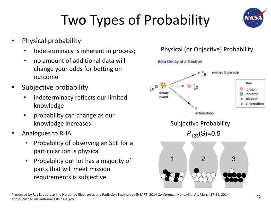
Two Types of Probability • Physical probability

• Indeterminacy is inherent in process; • no amount of additional data will

change your odds for betting on outcome

• Subjective probability • indeterminacy reflects our limited

knowledge • probability can change as our

knowledge increases • Analogues to RHA

• Probability of observing an SEE for a particular ion is physical

• Probability our lot has a majority of parts that will meet mission requirements is subjective

Physical (or Objective) Probability

Subjective Probability

13

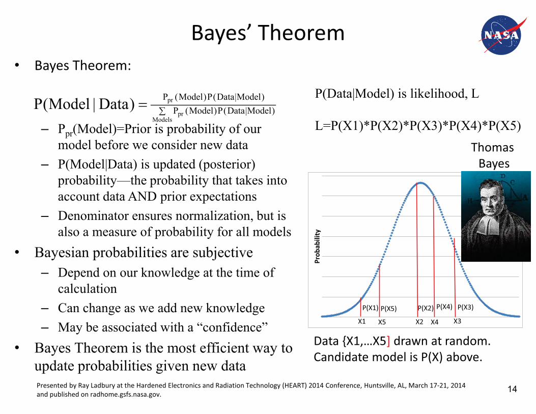
Bayes’ Theorem • Bayes Theorem:

– Ppr(Model)=Prior is probability of our model before we consider new data

– P(Model|Data) is updated (posterior) probability—the probability that takes into account data AND prior expectations

– Denominator ensures normalization, but is also a measure of probability for all models

• Bayesian probabilities are subjective– Depend on our knowledge at the time of

calculation– Can change as we add new knowledge– May be associated with a “confidence”

• Bayes Theorem is the most efficient way to update probabilities given new data

��Models

pr

pr

)Model|Data(P)Model(P)Model|Data(P)Model(P)Data|Model(P

Prob

abili

tyP(X1) P(X2) P(X3)P(X5) P(X4)

X1 X5 X3X2 X4

P(Data|Model) is likelihood, L

L=P(X1)*P(X2)*P(X3)*P(X4)*P(X5)Thomas

Bayes

Data {X1,…X5] drawn at random. Candidate model is P(X) above.


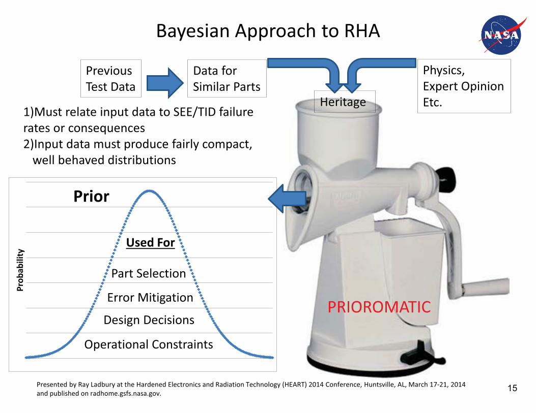
Bayesian Approach to RHA

PRIOROMATIC

Previous Test Data

Data for Similar Parts

Heritage

Physics, Expert Opinion Etc.

Prob

abili

ty

1)Must relate input data to SEE/TID failure rates or consequences 2)Input data must produce fairly compact, well behaved distributions

Used For

Part Selection

Error Mitigation

Design Decisions

Operational Constraints

Prior


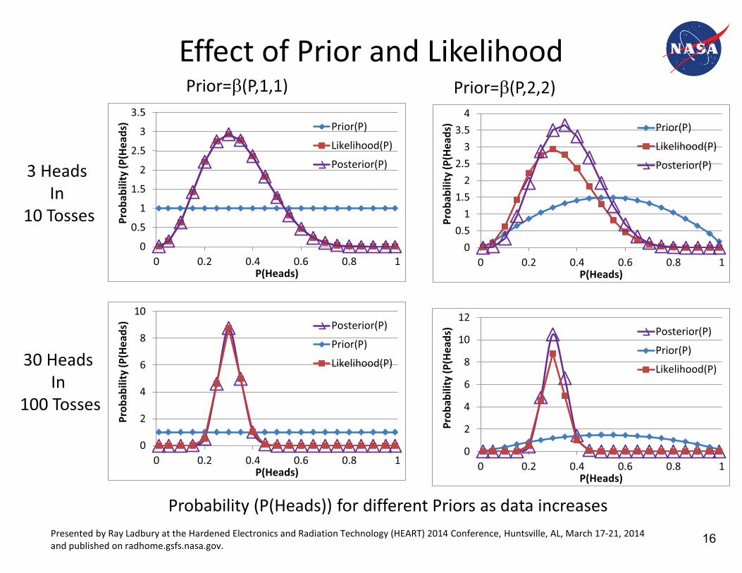
Effect of Prior and Likelihood

00.5

11.5

22.5

33.5

4

0 0.2 0.4 0.6 0.8 1

Prob

abili

ty (P

(Hea

ds)

P(Heads)

Prior(P)

Likelihood(P)

Posterior(P)

0

0.5

1

1.5

2

2.5

3

3.5

0 0.2 0.4 0.6 0.8 1

Prob

abili

ty (P

(Hea

ds)

P(Heads)

Prior(P)

Likelihood(P)

Posterior(P)

0

2

4

6

8

10

0 0.2 0.4 0.6 0.8 1

Prob

abili

ty (P

(Hea

ds)

P(Heads)

Posterior(P)

Prior(P)

Likelihood(P)

0

2

4

6

8

10

12

0 0.2 0.4 0.6 0.8 1

Prob

abili

ty (P

(Hea

ds)

P(Heads)

Posterior(P)

Prior(P)

Likelihood(P)

Prior=�(P,2,2)Prior=�(P,1,1)

3 Heads In

10 Tosses

30 Heads In

100 Tosses

Probability (P(Heads)) for different Priors as data increases Presented by Ray Ladbury at the Hardened Electronics and Radiation Technology (HEART) 2014 Conference, Huntsville, AL, March 17-21, 2014 and published on radhome.gsfs.nasa.gov. 16


Minimizing Subjectivity • Uninformative Priors—Broad, slowly varying (flat) Priors give rise to

Posterior distributions that reflect the data (likelihood) – If Prior is 0 anywhere, Posterior also 0 there (impossible means impossible) – Some Uninformative priors (for discrete distributions) are called Maximum

Entropy priors • Empirical Bayes allows looking at the data before developing Prior

– Can locate Prior at the maximum of the likelihood and make it very broad • This means you think the likelihood probably gives the best guess for the best fit,

but allow for significant sampling error • Usually yields good results unless there are serious sampling or systematic errors • Some Bayesians refer to this as “cheating”

• Maximize the data to update the Prior and dilute its influence. • Also, you don’t have to try only a single Prior—you could even attach prior

probabilities to your priors if you want to go really meta. Or you could try several Priors just to gauge the dependence of results on the Prior.

17

Data Sources

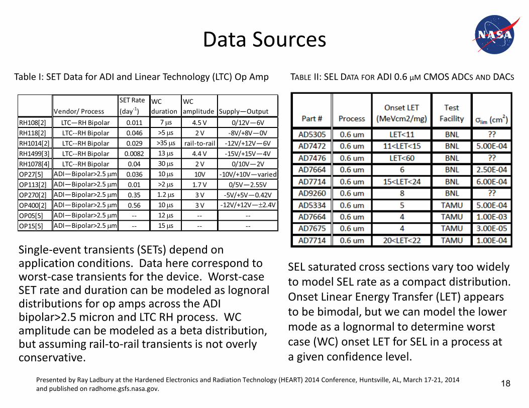
Single-event transients (SETs) depend on application conditions. Data here correspond to worst-case transients for the device. Worst-case SET rate and duration can be modeled as lognoral distributions for op amps across the ADI bipolar>2.5 micron and LTC RH process. WC amplitude can be modeled as a beta distribution, but assuming rail-to-rail transients is not overly conservative.

SEL saturated cross sections vary too widely to model SEL rate as a compact distribution. Onset Linear Energy Transfer (LET) appears to be bimodal, but we can model the lower mode as a lognormal to determine worst case (WC) onset LET for SEL in a process at a given confidence level.

Vendor/ Process

SET Rate (day-1)

WC duration

WC amplitude Supply�Output

RH108[2] �� 0.011 7 �s 4.5 V ��RH118[2] LTC--RH Bipolar 0.046 >5 �s 2 V ��RH1014[2] LTC--RH Bipolar 0.029 >35 �s rail-to-rail ��RH1499[3] LTC--RH Bipolar 0.0082 13 �s 4.4 V ��RH1078[4] LTC--RH Bipolar 0.04 30 �s 2 V ��OP27[5] �� m 0.036 10 �s 10V ��!��"$OP113[2] �� m 0.01 >2 �s 1.7 V ��OP270[2] �� m 0.35 1.2 �s 3 V ��OP400[2] �� m 0.56 10 �s 3 V ��2.4VOP05[5] �� m -- 12 �s -- --OP15[5] �� m -- 15 �s -- --

Table I: SET Data for ADI and Linear Technology (LTC) Op Amp TABLE II: SEL DATA FOR ADI 0.6 μM CMOS ADCS AND DACS


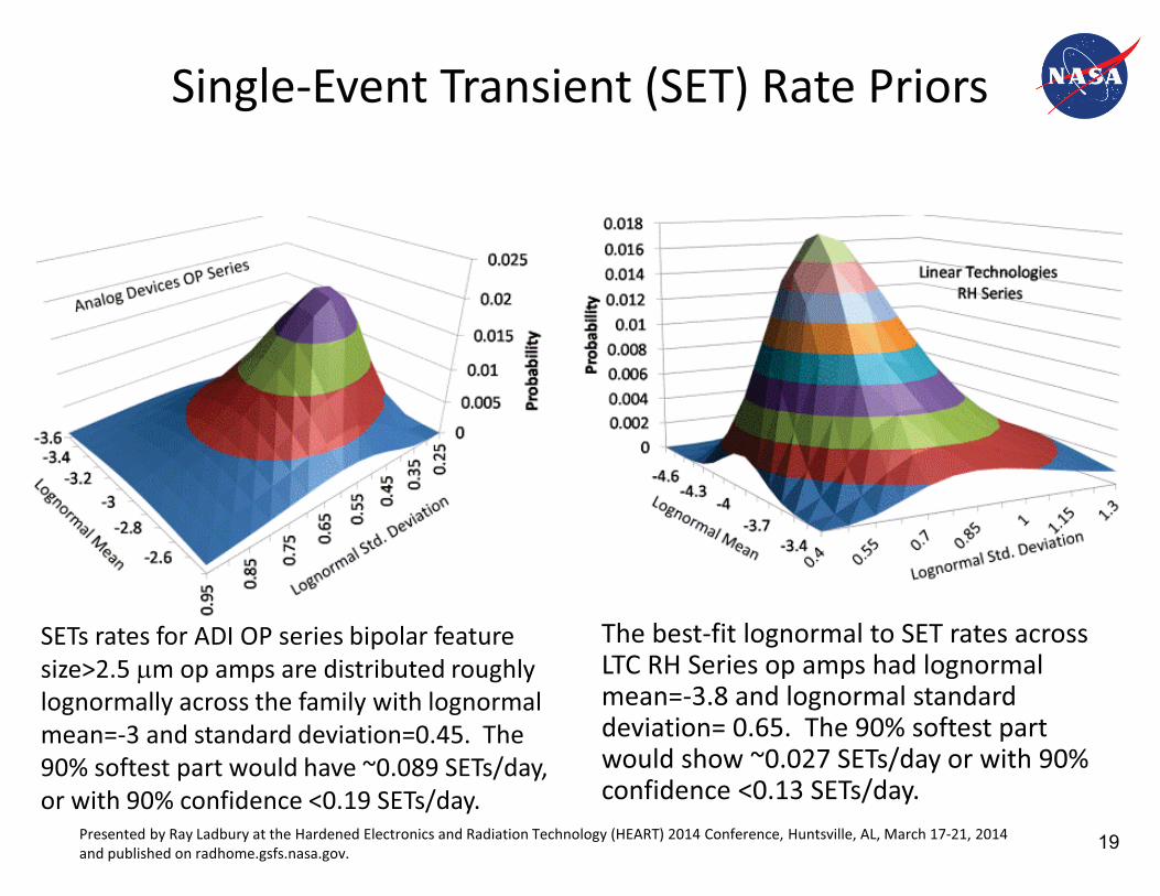
Single-Event Transient (SET) Rate Priors

SETs rates for ADI OP series bipolar feature size>2.5 �m op amps are distributed roughly lognormally across the family with lognormal mean=-3 and standard deviation=0.45. The 90% softest part would have ~0.089 SETs/day, or with 90% confidence <0.19 SETs/day.

The best-fit lognormal to SET rates across LTC RH Series op amps had lognormal mean=-3.8 and lognormal standard deviation= 0.65. The 90% softest part would show ~0.027 SETs/day or with 90% confidence <0.13 SETs/day.


SET Duration Priors

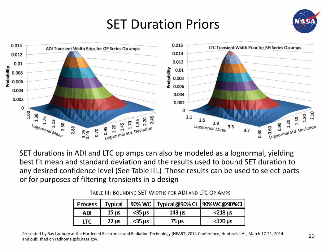
SET durations in ADI and LTC op amps can also be modeled as a lognormal, yielding best fit mean and standard deviation and the results used to bound SET duration to any desired confidence level (See Table III.) These results can be used to select parts or for purposes of filtering transients in a design

TABLE III: BOUNDING SET WIDTHS FOR ADI AND LTC OP AMPS


SEL Onset and Heritage

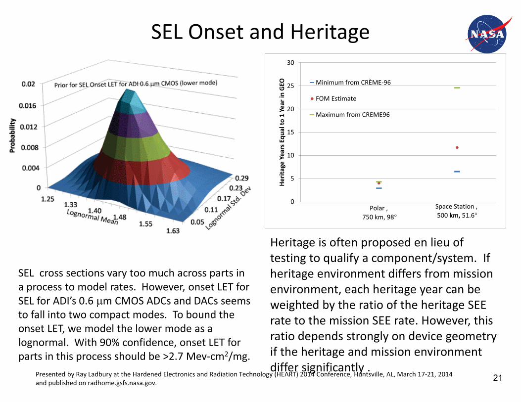
SEL cross sections vary too much across parts in a process to model rates. However, onset LET for SEL for ADI’s 0.6 �m CMOS ADCs and DACs seems to fall into two compact modes. To bound the onset LET, we model the lower mode as a lognormal. With 90% confidence, onset LET for parts in this process should be >2.7 Mev-cm2/mg.

Heritage is often proposed en lieu of testing to qualify a component/system. If heritage environment differs from mission environment, each heritage year can be weighted by the ratio of the heritage SEE rate to the mission SEE rate. However, this ratio depends strongly on device geometry if the heritage and mission environment differ significantly .

0

5

10

15

20

25

30

Herit

age

Year

s Equ

al to

1 Y

ear i

n G

EO Minimum from CRÈME-96

FOM Estimate

Maximum from CREME96

Polar , 750 km, 98

Space Station , 500 km, 51.6



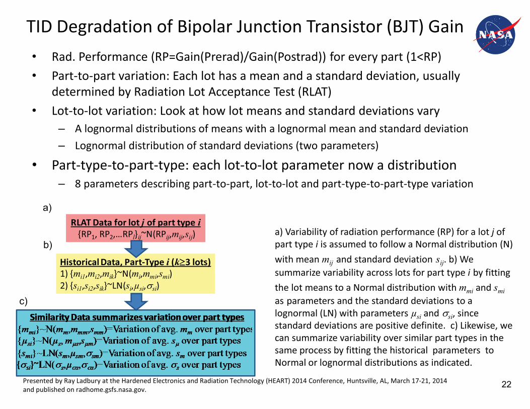
TID Degradation of Bipolar Junction Transistor (BJT) Gain • Rad. Performance (RP=Gain(Prerad)/Gain(Postrad)) for every part (1<RP) • Part-to-part variation: Each lot has a mean and a standard deviation, usually

determined by Radiation Lot Acceptance Test (RLAT) • Lot-to-lot variation: Look at how lot means and standard deviations vary

– A lognormal distributions of means with a lognormal mean and standard deviation – Lognormal distribution of standard deviations (two parameters)

• Part-type-to-part-type: each lot-to-lot parameter now a distribution – 8 parameters describing part-to-part, lot-to-lot and part-type-to-part-type variation

RLAT Data for lot j of part type i

{RP1, RP2,…RPl}ij~N(RPij,mij,sij)

Historical Data, Part-Type i (k3 lots)1) {mi1,mi2,mik}~N(mi,mmi,smi)2) {si1,si2,sik}~LN(si,µsi,�si)

a)

b)

c)

a) Variability of radiation performance (RP) for a lot j of part type i is assumed to follow a Normal distribution (N) with mean mij and standard deviation sij. b) We summarize variability across lots for part type i by fitting the lot means to a Normal distribution with mmi and smi as parameters and the standard deviations to a lognormal (LN) with parameters µsi and �si, since standard deviations are positive definite. c) Likewise, we can summarize variability over similar part types in the same process by fitting the historical parameters to Normal or lognormal distributions as indicated.

22


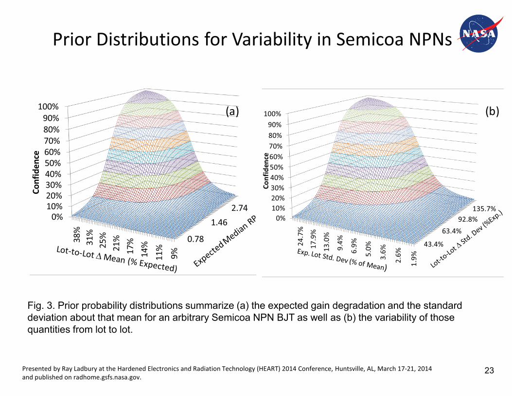
Prior Distributions for Variability in Semicoa NPNs

1.9%2.6%3.6%5.0%6.9%9.4%

13.0

%

17.9

%

24.7

%

0%10%20%30%40%50%60%70%80%90%

100%

43.4%

63.4%92.8%

135.7%

Conf

iden

ce

(b)

9%11%

14%

17%

21%

25%

31%

38%

0%10%20%30%40%50%60%70%80%90%

100%

0.78

1.462.74

Conf

iden

ce

(a)

Fig. 3. Prior probability distributions summarize (a) the expected gain degradation and the standard deviation about that mean for an arbitrary Semicoa NPN BJT as well as (b) the variability of those quantities from lot to lot.

23

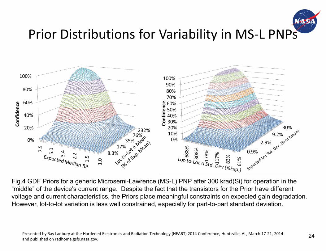
Prior Distributions for Variability in MS-L PNPs

Fig.4 GDF Priors for a generic Microsemi-Lawrence (MS-L) PNP after 300 krad(Si) for operation in the “middle” of the device’s current range. Despite the fact that the transistors for the Prior have different voltage and current characteristics, the Priors place meaningful constraints on expected gain degradation. However, lot-to-lot variation is less well constrained, especially for part-to-part standard deviation.

61%83%

117%178%308%688%

0%10%20%30%40%50%60%70%80%90%

100%

0.9%

2.9%9.2%

30%Conf

iden

ce

1.01.

52.23.

45.07.5

0%

20%

40%

60%

80%

100%

8.3%17%

35%76%

232%

Conf

iden

ce



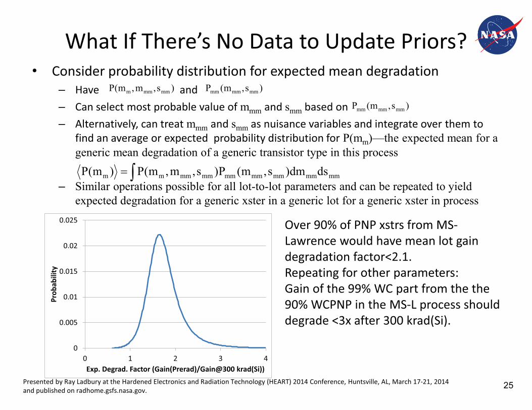
What If There’s No Data to Update Priors? • Consider probability distribution for expected mean degradation

– Have and – Can select most probable value of mmm and smm based on – Alternatively, can treat mmm and smm as nuisance variables and integrate over them to

find an average or expected probability distribution for P(mm)—the expected mean for a generic mean degradation of a generic transistor type in this process

– Similar operations possible for all lot-to-lot parameters and can be repeated to yield expected degradation for a generic xster in a generic lot for a generic xster in process

�� mmmmmmmmmmmmmmmm dsdm)s,m(P)s,m,m(P)m(P

)s,m,m(P mmmmm )s,m(P mmmmmm

)s,m(P mmmmmm

0

0.005

0.01

0.015

0.02

0.025

0 1 2 3 4

Prob

abili

ty

Exp. Degrad. Factor (Gain(Prerad)/Gain@300 krad(Si))

Over 90% of PNP xstrs from MS- Lawrence would have mean lot gain degradation factor<2.1. Repeating for other parameters: Gain of the 99% WC part from the the 90% WCPNP in the MS-L process should degrade <3x after 300 krad(Si).

25

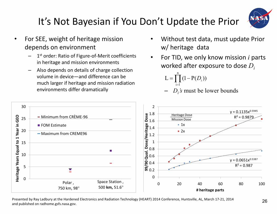
It’s Not Bayesian if You Don’t Update the Prior • Without test data, must update Prior

w/ heritage data • For TID, we only know mission i parts

worked after exposure to dose Di

– Di’s must be lower bounds

))(P1(Ln

1i��

� iD

y = 0.0651x0.5387

R² = 0.987

y = 0.1135x0.5945

R² = 0.9879

0

0.2

0.4

0.6

0.8

1

1.2

1.4

1.6

1.8

2

0 20 40 60 80 100

99/9

0 Q

ual.

Dose

/Her

itage

Dos

e

# heritage parts

1x2x

Heritage DoseMission Dose

• For SEE, weight of heritage mission depends on environment

– 1st order: Ratio of Figure-of-Merit coefficients in heritage and mission environments

– Also depends on details of charge collection volume in device—and difference can be much larger if heritage and mission radiation environments differ dramatically

0

5

10

15

20

25

30

Herit

age

Year

s Equ

al to

1 Y

ear i

n G

EO Minimum from CRÈME-96

FOM Estimate

Maximum from CREME96

Polar , 750 km, 98

Space Station , 500 km, 51.6


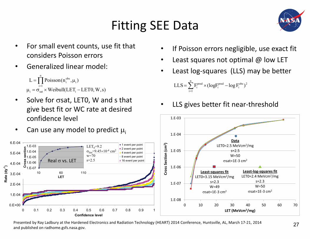
Fitting SEE Data

2obsi

predi

n

1i

predi )FlogF(logFLLS ��

�

• If Poisson errors negligible, use exact fit • Least squares not optimal @ low LET • Least log-squares (LLS) may be better

• LLS gives better fit near-threshold

1.E-08

1.E-07

1.E-06

1.E-05

1.E-04

1.E-03

0 10 20 30 40 50 60 70

Cros

s Sec

tion

(cm

2 )

LET (MeVcm2/mg)

Least-squares fitLET0=3.15 MeVcm2/mg

s=2.3W=49

�sat=1E-3 cm2

Least-log-squares fitLET0=2.4 MeVcm2/mg

s=2.3W=50

�sat=1E-3 cm2

DataLET0=2.5 MeVcm2/mg

s=2.5W=50

�sat=1E-3 cm2

• For small event counts, use fit that considers Poisson errors

• Generalized linear model:

• Solve for �sat, LET0, W and s that

give best fit or WC rate at desired confidence level

• Can use any model to predict �i

0.E+00

1.E-04

2.E-04

3.E-04

4.E-04

5.E-04

6.E-04

0 0.1 0.2 0.3 0.4 0.5 0.6 0.7 0.8 0.9 1Confidence level

Rat

e (d

y-1)

1 event per point2 event per point4 event per point8 event per point16 event per point

1.E-07

1.E-06

1.E-05

1.E-04

1.E-03

10 60 110LET

Cro

ss s

ectio

n LET0=9.2�lim=9.45�10-4 cm2

w=70s=2.5

),n(PoissonL i

n

1i

obsi ��

�)s,W,0LETLET(Weibull isati ��


Real � vs. LET

27

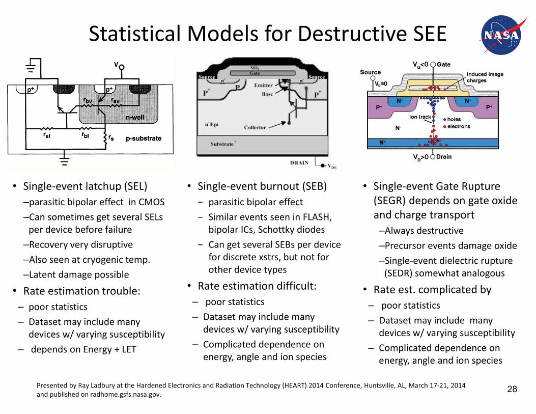
Statistical Models for Destructive SEE

• Single-event latchup (SEL) –parasitic bipolar effect in CMOS –Can sometimes get several SELs

per device before failure –Recovery very disruptive –Also seen at cryogenic temp. –Latent damage possible

• Rate estimation trouble: – poor statistics – Dataset may include many

devices w/ varying susceptibility – depends on Energy + LET

• Single-event Gate Rupture (SEGR) depends on gate oxide and charge transport –Always destructive –Precursor events damage oxide –Single-event dielectric rupture

(SEDR) somewhat analogous

• Rate est. complicated by – poor statistics – Dataset may include many

devices w/ varying susceptibility – Complicated dependence on

energy, angle and ion species

• Single-event burnout (SEB) & parasitic bipolar effect & Similar events seen in FLASH,

bipolar ICs, Schottky diodes & Can get several SEBs per device

for discrete xstrs, but not for other device types

• Rate estimation difficult: – poor statistics – Dataset may include many

devices w/ varying susceptibility – Complicated dependence on

energy, angle and ion species


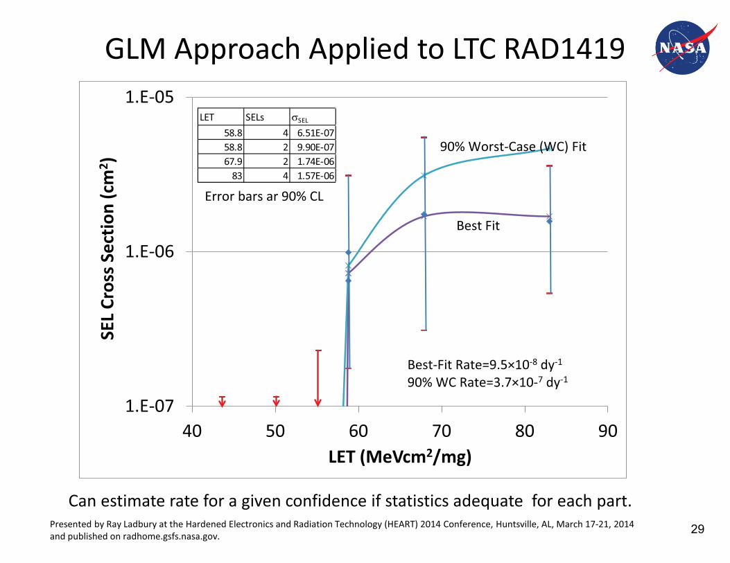
GLM Approach Applied to LTC RAD1419

1.E-07

1.E-06

1.E-05

40 50 60 70 80 90

SEL

Cros

s Sec

tion

(cm

2 )

LET (MeVcm2/mg)

Best Fit

90% Worst-Case (WC) Fit

LET SELs �SEL

58.8 4 6.51E-0758.8 2 9.90E-0767.9 2 1.74E-06

83 4 1.57E-06

Error bars ar 90% CL

Best-Fit Rate=9.5×10-8 dy-1

90% WC Rate=3.7×10-7 dy-1

Can estimate rate for a given confidence if statistics adequate for each part. Presented by Ray Ladbury at the Hardened Electronics and Radiation Technology (HEART) 2014 Conference, Huntsville, AL, March 17-21, 2014 and published on radhome.gsfs.nasa.gov. 29


Limitations of GLM for Destructive SEE

• GLM technique works well when statistics accumulated for each test device – Allows bounding of rate for a given confidence level – Flexible and can be adapted to include other sources of error – Model need not be standard Weibull rectangular parallelepiped

• Could even be Monte Carlo output for several geometric models of sensitive volume

• Unfortunately, for some device types, every event kills a part – SEGR is always destructive to power Metal-Oxide-Semiconductor Field Effect

Transistor (MOSFET) as are failures in FLASH, bipolar microcircuits and diodes – Accumulating statistics done over several parts

• How do you detect/treat part-to-part variation

• Even if statistics gathered for each device, susceptibility can change w/ time – TID can alter susceptibility – Latent damage due to overcurrent (SEL, SEB, etc.) or bus contention due to SEE – Complex devices may have different susceptibilities during different

• How do we deal with Poisson error, part-to-part variation and time dependent susceptibility—possibly all at the same time?

30


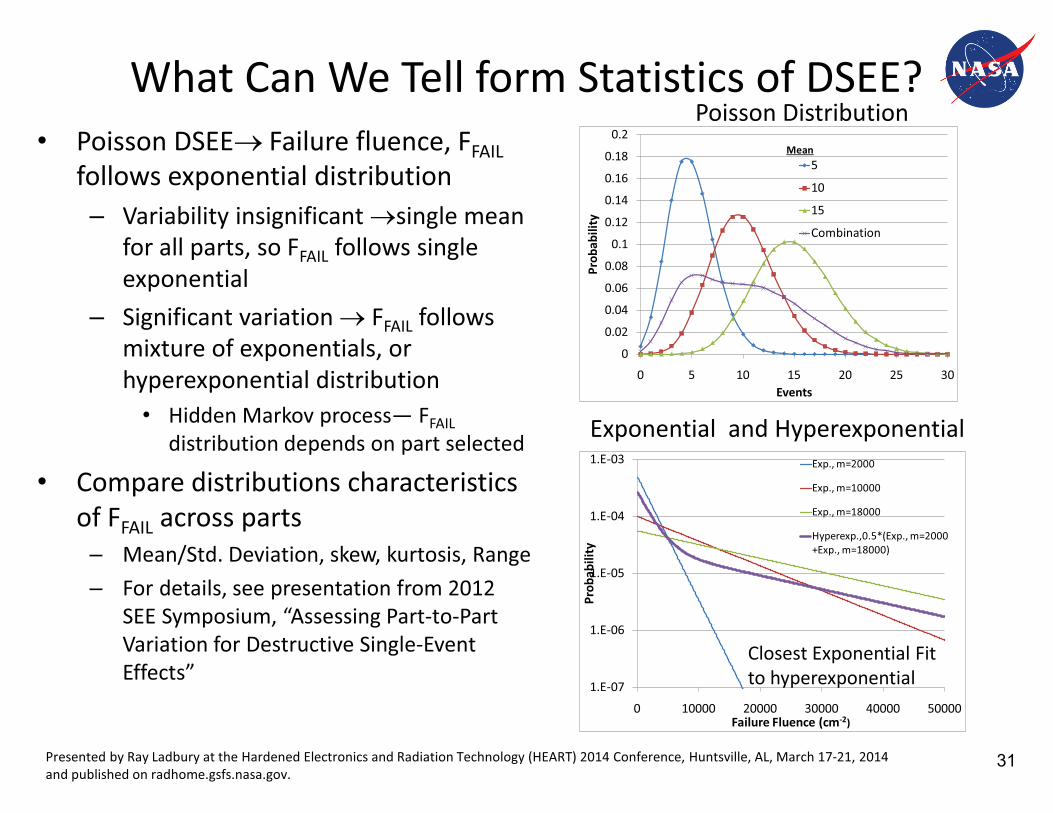
What Can We Tell form Statistics of DSEE? • Poisson DSEE� Failure fluence, FFAIL

follows exponential distribution – Variability insignificant �single mean

for all parts, so FFAIL follows single exponential

– Significant variation � FFAIL follows mixture of exponentials, or hyperexponential distribution

• Hidden Markov process— FFAIL distribution depends on part selected

• Compare distributions characteristics of FFAIL across parts

– Mean/Std. Deviation, skew, kurtosis, Range – For details, see presentation from 2012

SEE Symposium, “Assessing Part-to-Part Variation for Destructive Single-Event Effects”

Poisson Distribution

Exponential and Hyperexponential

0

0.02

0.04

0.06

0.08

0.1

0.12

0.14

0.16

0.18

0.2

0 5 10 15 20 25 30

Prob

abili

ty

Events

5

10

15

Combination

Mean

1.E-07

1.E-06

1.E-05

1.E-04

1.E-03

0 10000 20000 30000 40000 50000

Prob

abili

ty

Failure Fluence (cm-2)

Exp., m=2000

Exp., m=10000

Exp., m=18000

Hyperexp.,0.5*(Exp., m=2000 +Exp., m=18000)

Closest Exponential Fit to hyperexponential

31

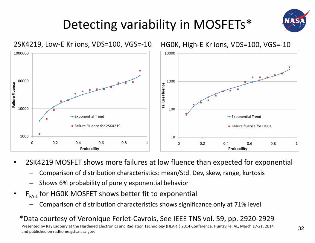
Detecting variability in MOSFETs*

1000

10000

100000

1000000

0 0.2 0.4 0.6 0.8 1

Failu

re Fl

uenc

e

Probability

Exponential Trend

Failure Fluence for 2SK4219

10

100

1000

10000

0 0.2 0.4 0.6 0.8 1

Failu

re Fl

uenc

e

Probability

Exponential Trend

Failure fluence for HG0K

2SK4219, Low-E Kr ions, VDS=100, VGS=-10 HG0K, High-E Kr ions, VDS=100, VGS=-10

• 2SK4219 MOSFET shows more failures at low fluence than expected for exponential – Comparison of distribution characteristics: mean/Std. Dev, skew, range, kurtosis – Shows 6% probability of purely exponential behavior

• FFAIL for HG0K MOSFET shows better fit to exponential – Comparison of distribution characteristics shows significance only at 71% level

*Data courtesy of Veronique Ferlet-Cavrois, See IEEE TNS vol. 59, pp. 2920-2929 Presented by Ray Ladbury at the Hardened Electronics and Radiation Technology (HEART) 2014 Conference, Huntsville, AL, March 17-21, 2014 and published on radhome.gsfs.nasa.gov. 32


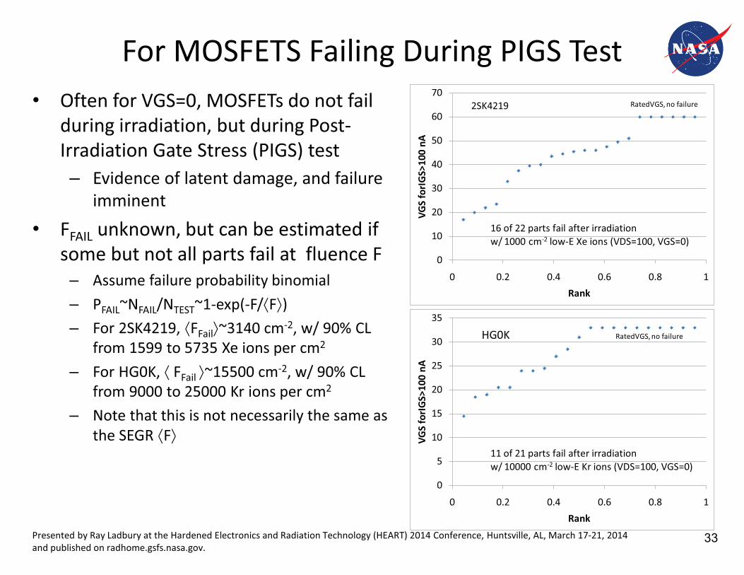
For MOSFETS Failing During PIGS Test • Often for VGS=0, MOSFETs do not fail

during irradiation, but during Post-Irradiation Gate Stress (PIGS) test – Evidence of latent damage, and failure

imminent • FFAIL unknown, but can be estimated if

some but not all parts fail at fluence F – Assume failure probability binomial – PFAIL~NFAIL/NTEST~1-exp(-F/�F�) – For 2SK4219, �FFail�~3140 cm-2, w/ 90% CL

from 1599 to 5735 Xe ions per cm2

– For HG0K, � FFail �~15500 cm-2, w/ 90% CL from 9000 to 25000 Kr ions per cm2

– Note that this is not necessarily the same as the SEGR �F�

0

10

20

30

40

50

60

70

0 0.2 0.4 0.6 0.8 1

VGS

forIG

S>10

0 nA

Rank

RatedVGS, no failure

16 of 22 parts fail after irradiation w/ 1000 cm-2 low-E Xe ions (VDS=100, VGS=0)

2SK4219

0

5

10

15

20

25

30

35

0 0.2 0.4 0.6 0.8 1

VGS

forIG

S>10

0 nA

Rank

RatedVGS, no failure

11 of 21 parts fail after irradiation w/ 10000 cm-2 low-E Kr ions (VDS=100, VGS=0)

HG0K

33

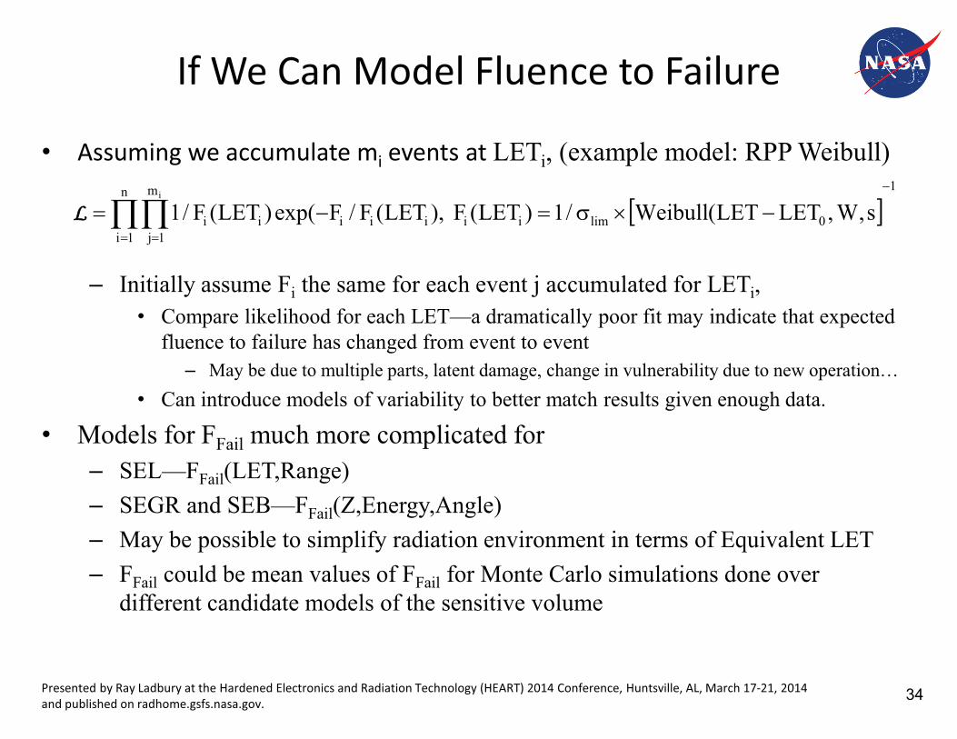
If We Can Model Fluence to Failure

• Assuming we accumulate mi events at LETi, (example model: RPP Weibull)

– Initially assume Fi the same for each event j accumulated for LETi,• Compare likelihood for each LET—a dramatically poor fit may indicate that expected

fluence to failure has changed from event to event– May be due to multiple parts, latent damage, change in vulnerability due to new operation…

• Can introduce models of variability to better match results given enough data.

• Models for FFail much more complicated for – SEL—FFail(LET,Range)– SEGR and SEB—FFail(Z,Energy,Angle)– May be possible to simplify radiation environment in terms of Equivalent LET– FFail could be mean values of FFail for Monte Carlo simulations done over

different candidate models of the sensitive volume

� �1n

1i0limiiiii

m

1jii s,W,LETLET(Weibull/1)LET(F),LET(F/Fexp()LET(F/1

i

� �� LL



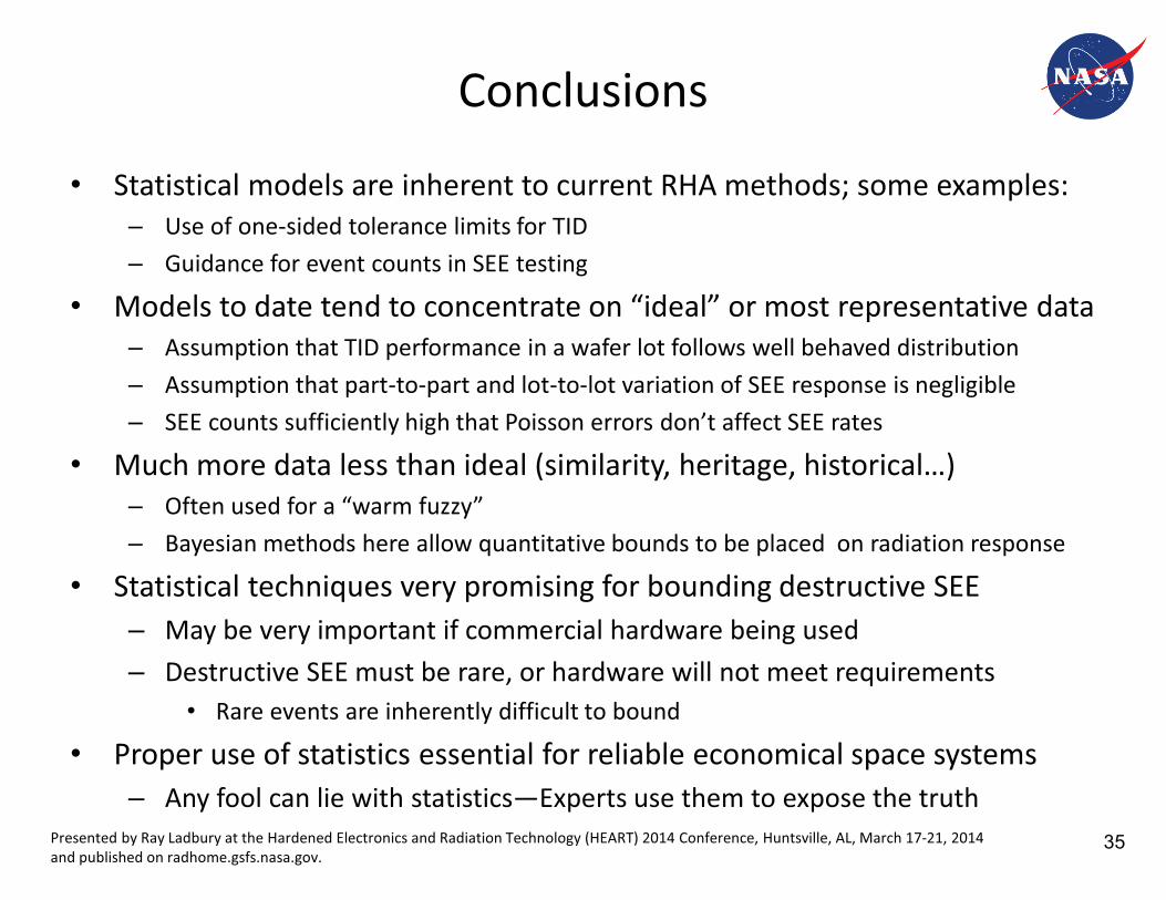
Conclusions

• Statistical models are inherent to current RHA methods; some examples: – Use of one-sided tolerance limits for TID – Guidance for event counts in SEE testing

• Models to date tend to concentrate on “ideal” or most representative data – Assumption that TID performance in a wafer lot follows well behaved distribution – Assumption that part-to-part and lot-to-lot variation of SEE response is negligible – SEE counts sufficiently high that Poisson errors don’t affect SEE rates

• Much more data less than ideal (similarity, heritage, historical…) – Often used for a “warm fuzzy” – Bayesian methods here allow quantitative bounds to be placed on radiation response

• Statistical techniques very promising for bounding destructive SEE– May be very important if commercial hardware being used – Destructive SEE must be rare, or hardware will not meet requirements

• Rare events are inherently difficult to bound

• Proper use of statistics essential for reliable economical space systems – Any fool can lie with statistics—Experts use them to expose the truth

35

Documents

Statistical Modeling for Radiation Hardness Assurance … · Statistical Modeling for Radiation Hardness Assurance ... 0.030 0.035 0.040 ... Statistical Modeling for Radiation Hardness