Statistical Methods for Quality Control - Cengage Methods for Quality Control CONTENTS STATISTICS IN PRACTICE: DOW CHEMICAL COMPANy 15.1 PHILOSOPHIES AND fRAMEWORkS …

Statistical Methods for Quality Control

CONTENTS

STATISTICS IN PRACTICE: DOW CHEMICAL COMPANy

15.1 PHILOSOPHIES AND fRAMEWORkSMalcolm Baldrige National

Quality AwardISO 9000Six SigmaQuality in the Service Sector

15.2 STATISTICAL PROCESS CONTROLControl Chartsx Chart: Process Mean and

Standard Deviation known

x Chart: Process Mean and Standard Deviation Unknown

R Chartp Chartnp ChartInterpretation of Control Charts

15.3 ACCEPTANCE SAMPLINGkALI, Inc.: An Example of

Acceptance SamplingComputing the Probability of

Accepting a LotSelecting an Acceptance

Sampling PlanMultiple Sampling Plans

CHAPTER 15

67045_ch15_ptg01_Web.indd 737 21/10/14 1:22 PM

738 Chapter 15 Statistical Methods for Quality Control

The American Society for Quality (ASQ) defines quality as “the totality of features and characteristics of a product or service that bears on its ability to satisfy given needs.” In other words, quality measures how well a product or service meets customer needs. Organiza-tions recognize that to be competitive in today’s global economy, they must strive for a high level of quality. As a result, they place increased emphasis on methods for monitoring and maintaining quality.

Today, the customer-driven focus that is fundamental to high-performing organizations has changed the scope that quality issues encompass, from simply eliminating defects on a production line to developing broad-based corporate quality strategies. Broadening the scope of quality naturally leads to the concept of total quality (TQ).

ASQ’s Vision: “By making quality a global priority, an organizational imperative, and a personal ethic, the American Society for Qual-ity becomes the community for everyone who seeks quality concepts, technol-ogy, and tools to improve themselves and their world” (ASQ website).

In 1940 the Dow Chemical Company purchased 800 acres of Texas land on the Gulf Coast to build a magne-sium production facility. That original site has expanded to cover more than 5000 acres and holds one of the larg-est petrochemical complexes in the world. Among the products from Dow Texas Operations are magnesium, styrene, plastics, adhesives, solvent, glycol, and chlorine. Some products are made solely for use in other processes, but many end up as essential ingredients in products such as pharmaceuticals, toothpastes, dog food, water hoses, ice chests, milk cartons, garbage bags, shampoos, and furniture.

Dow’s Texas Operations produce more than 30% of the world’s magnesium, an extremely lightweight metal used in products ranging from tennis racquets to suitcases to “mag” wheels. The Magnesium Depart-ment was the first group in Texas Operations to train its technical people and managers in the use of statistical quality control. Some of the earliest successful appli-cations of statistical quality control were in chemical processing.

In one application involving the operation of a drier, samples of the output were taken at periodic intervals; the average value for each sample was computed and recorded on a chart called an x chart. Such a chart enabled Dow analysts to monitor trends in the output that might indicate the process was not operating correctly. In one instance, analysts began to observe values for the sample mean that

were not indicative of a process operating within its design limits. On further examination of the control chart and the operation itself, the analysts found that the variation could be traced to problems involving one operator. The x chart recorded after retraining the operator showed a significant improve ment in the process quality.

Dow achieves quality improvements everywhere it applies statistical quality control. Documented savings of several hundred thousand dollars per year are realized, and new applications are continually being discovered.

In this chapter we will show how an x chart such as the one used by Dow can be developed. Such charts are a part of statistical quality control known as statistical process control. We will also discuss methods of quality control for situ ations in which a decision to accept or reject a group of items is based on a sample.

DOW CHEMICAL COMPANy*FReepoRt, texAS

STATISTICS in PRACTICE

*The authors are indebted to Clifford B. Wilson, Magnesium Technical Manager, The Dow Chemical Company, for providing this Statistics in Practice.

Statistical quality control has enabled Dow Chemical Company to improve its processing methods and output. © Bill Pugliano/Getty Images.

67045_ch15_ptg01_Web.indd 738 21/10/14 1:22 PM

15.1 Philosophies and Frameworks 739

1J. R. Evans and W. M. Lindsay, Managing for Quality and Performance Excellence, 8th ed. (Cincinnati, OH: Cengage Learning, 2011), p. 11.

Total Quality (TQ) is a people-focused management system that aims at continual increase in customer satisfaction at continually lower real cost. TQ is a total system approach (not a separate area or work program) and an integral part of high-level strategy; it works horizon-tally across function and departments, involves all employees, top to bottom, and extends backward and forward to include the supply chain and the customer chain. TQ stresses learning and adaptation to continual change as keys to organization success.1

Regardless of how it is implemented in different organizations, total quality is based on three fundamental principles: a focus on customers and stakeholders; participation and teamwork throughout the organization; and a focus on continuous improvement and learn-ing. In the first section of the chapter we provide a brief introduction to three quality management frameworks: the Malcolm Baldrige Quality Award, ISO 9000 standards, and the Six Sigma philosophy. In the last two sections we introduce two statistical tools that can be used to monitor quality: statistical process control and acceptance sampling.

15.1 Philosophies and FrameworksIn the early twentieth century, quality control practices were limited to inspecting fin-ished products and removing defective items. But this all changed as the result of the pioneering efforts of a young engineer named Walter A. Shewhart. After completing his doctorate in physics from the University of California in 1917, Dr. Shewhart joined the Western Electric Company, working in the inspection engineering department. In 1924 Dr. Shewhart prepared a memorandum that included a set of principles that are the basis for what is known today as process control. And his memo also contained a diagram that would be recognized as a statistical control chart. Continuing his work in quality at Bell Telephone Laboratories until his retirement in 1956, he brought together the disciplines of statistics, engineering, and economics and in doing so changed the course of industrial history. Dr. Shewhart is recognized as the father of statistical quality control and was the first honorary member of the ASQ.

Two other individuals who have had great influence on quality are Dr. W. Edwards Deming, a student of Dr. Shewhart, and Joseph Juran. These men helped educate the Japa-nese in quality management shortly after World War II. Although quality is everybody’s job, Deming stressed that the focus on quality must be led by managers. He developed a list of 14 points that he believed represent the key responsibilities of managers. for instance, Deming stated that managers must cease dependence on mass inspection; must end the practice of awarding business solely on the basis of price; must seek continual improvement in all production processes and service; must foster a team-oriented environment; and must eliminate goals, slogans, and work standards that prescribe numerical quotas. Perhaps most important, managers must create a work environment in which a commitment to quality and productivity is maintained at all times.

Juran proposed a simple definition of quality: fitness for use. Juran’s approach to qual-ity focused on three quality processes: quality planning, quality control, and quality im-provement. In contrast to Deming’s philosophy, which required a major cultural change in the organization, Juran’s programs were designed to improve quality by working within the current organizational system. Nonetheless, the two philosophies are similar in that they both focus on the need for top management to be involved and stress the need for continu-ous improvement, the importance of training, and the use of quality control techniques.

Many other individuals played significant roles in the quality movement, includ-ing Philip B. Crosby, A. V. feigenbaum, karou Ishikawa, and Genichi Taguchi. More

After World War II, Dr. W. edwards Deming became a consultant to Japanese industry; he is credited with being the person who convinced top managers in Japan to use the methods of statistical quality control.

67045_ch15_ptg01_Web.indd 739 21/10/14 1:22 PM


specialized texts dealing exclusively with quality provide details of the contributions of each of these individuals. The contributions of all individuals involved in the quality move-ment helped define a set of best practices and led to numerous awards and certification programs. The two most significant programs are the U.S. Malcolm Baldrige National Quality Award and the international ISO 9000 certification process. In recent years, use of Six Sigma—a methodology for improving organizational performance based on rigorous data collection and statistical analysis—has also increased.

Malcolm Baldrige National Quality AwardThe Malcolm Baldrige National Quality Award is given by the president of the United States to organizations that apply and are judged to be outstanding in seven areas: leader-ship; strategic planning; customer and market focus; measurement, analysis, and knowledge management; human resource focus; process management; and business results. Congress established the award program in 1987 to recognize U.S. organizations for their achieve-ments in quality and performance and to raise awareness about the importance of quality as a competitive edge. The award is named for Malcolm Baldrige, who served as secretary of commerce from 1981 until his death in 1987.

Since the presentation of the first awards in 1988, the Baldrige National Quality Pro-gram (BNQP) has grown in stature and impact. Approximately 2 million copies of the criteria have been distributed since 1988, and wide-scale reproduction by organizations and electronic access add to that number significantly. for eight years in a row, a hypothetical stock index, made up of publicly traded U.S. companies that had received the Baldrige Award, outperformed the Standard & Poor’s 500. In one year, the “Baldrige Index” outper-formed the S&P 500 by 4.4 to 1. Bob Barnett, executive vice presi dent of Motorola, Inc., said, “We applied for the Award, not with the idea of winning, but with the goal of receiv-ing the evaluation of the Baldrige Examiners. That evaluation was comprehensive, profes-sional, and insightful . . . making it perhaps the most cost- effective, value-added business consultation available anywhere in the world today.”

ISO 9000ISO 9000 is a series of five international standards published in 1987 by the International Organization for Standardization (ISO), Geneva, Switzerland. Companies can use the standards to help determine what is needed to maintain an efficient quality conformance system. for example, the standards describe the need for an effective quality system, for ensuring that measuring and testing equipment is calibrated regularly, and for maintaining an adequate record-keeping system. ISO 9000 registration determines whether a company complies with its own quality system. Overall, ISO 9000 registration covers less than 10% of the Baldrige Award criteria.

Six SigmaIn the late 1980s Motorola recognized the need to improve the quality of its products and services; its goal was to achieve a level of quality so good that for every million oppor-tunities no more than 3.4 defects will occur. This level of quality is referred to as the six sigma level of quality, and the methodology created to reach this quality goal is referred to as Six Sigma.

An organization may undertake two kinds of Six Sigma projects:

DMAIC (Define, Measure, Analyze, Improve, and Control) to help redesign exist-ing processes

DfSS (Design for Six Sigma) to design new products, processes, or services

the U.S. Commerce Department’s National Institute of Standards and technology (NISt) man-ages the Baldrige National Quality program. More in-formation can be obtained at the NISt website.

2004 was the final year for the Baldrige Stock Study because of the increase in the number of recipients that are either nonprofit or privately held businesses.

ISo 9000 standards are revised periodically to improve the quality of the standard.

67045_ch15_ptg01_Web.indd 740 21/10/14 1:22 PM

15.1 Philosophies and Frameworks 741

In helping to redesign existing processes and design new processes, Six Sigma places a heavy emphasis on statistical analysis and careful measurement. Today, Six Sigma is a major tool in helping organizations achieve Baldrige levels of business performance and process quality. Many Baldrige examiners view Six Sigma as the ideal approach for imple-menting Baldrige improvement programs.

Six Sigma limits and defects per million opportunities In Six Sigma terminology, a defect is any mistake or error that is passed on to the customer. The Six Sigma process defines quality performance as defects per million opportunities (dpmo). As we indicated previously, Six Sigma represents a quality level of at most 3.4 dpmo. To illustrate how this quality level is measured, let us consider the situation at kJW Packaging.

kJW operates a production line where boxes of cereal are filled. The filling pro-cess has a mean of μ 5 16.05 ounces and a standard deviation of σ 5 .10 ounces. It is reasonable to assume the filling weights are normally distributed. The distribution of filling weights is shown in figure 15.1. Suppose management considers 15.45 to 16.65 ounces to be acceptable quality limits for the filling process. Thus, any box of cereal that contains less than 15.45 or more than 16.65 ounces is considered to be a defect. Using Excel, it can be shown that 99.9999998% of the boxes filled will have between 16.05 2 6(.10) 5 15.45 ounces and 16.05 1 6(.10) 5 16.65 ounces. In other words, only .0000002% of the boxes filled will contain less than 15.45 ounces or more than 16.65 ounces. Thus, the likelihood of obtaining a defective box of cereal from the fill-ing process appears to be extremely unlikely, because on average only two boxes in 10 million will be defective.

Motorola’s early work on Six Sigma convinced Motorola’s managers that a process mean can shift on average by as much as 1.5 standard deviations. for in-stance, suppose that the process mean for kJW increases by 1.5 standard deviations or 1.5(.10) 5 .15 ounces. With such a shift, the normal distribution of filling weights would now be centered at μ 5 16.05 1 .15 5 16.20 ounces. With a process mean of μ 5 16.05 ounces, the probability of obtaining a box of cereal with more than 16.65 ounces is extremely small. But how does this probability change if the mean

Using excel, NoRM.S.DISt (6,tRUe) 2 NoRM.S.DISt (26,tRUe) 5 .999999998.

Using excel, 1 2 NoRM.S.DISt (4.5,tRUe)5 .0000034.

16.0515.45Lower quality

limit

16.65Upper quality

limit

� 5 .10

Process mean

Defect Defect

�

FIGURE 15.1 NORMAL DISTRIBUTION Of CEREAL BOX fILLING WEIGHTS WITH A PROCESS MEAN μ 5 16.05

67045_ch15_ptg01_Web.indd 741 21/10/14 1:22 PM


of the process shifts up to μ 5 16.20 ounces? figure 15.2 shows that for this case, the upper quality limit of 16.65 is 4.5 standard deviations to the right of the new mean μ 5 16.20 ounces. Using this mean and Excel, we find that the probability of obtaining a box with more than 16.65 ounces is .0000034. Thus, if the process mean shifts up by 1.5 standard deviations, approximately 1,000,000(.0000034) 5 3.4 boxes of cereal will exceed the upper limit of 16.65 ounces. In Six Sigma terminology, the quality level of the process is said to be 3.4 defects per million opportunities. If management of kJW considers 15.45 to 16.65 ounces to be acceptable quality lim-its for the filling process, the kJW filling process would be considered a Six Sigma process. Thus, if the process mean stays within 1.5 standard deviations of its target value μ 5 16.05 ounces, a maximum of only 3.4 defects per million boxes filled can be expected.

Organizations that want to achieve and maintain a Six Sigma level of quality must emphasize methods for monitoring and maintaining quality. Quality assurance refers to the entire system of policies, procedures, and guidelines established by an organization to achieve and maintain quality. Quality assurance consists of two principal functions: quality engineering and quality control. The object of quality engineering is to include quality in the design of products and processes and to identify quality problems prior to production. Quality control consists of a series of inspections and measurements used to determine whether quality standards are being met. If quality standards are not being met, correc-tive or preventive action can be taken to achieve and maintain conformance. In the next two sections we present two statistical methods used in quality control. The first method, statistical process control, uses graphical displays known as control charts to monitor a process; the goal is to determine whether the process can be continued or whether corrective action should be taken to achieve a desired quality level. The second method, acceptance sampling, is used in situations where a decision to accept or reject a group of items must be based on the quality found in a sample.

5 16.20 16.65Upper quality

limit

� 5 .10

Process mean increasesby 1.5 standard deviations

.0000034 or3.4 dpmo

�

FIGURE 15.2 NORMAL DISTRIBUTION Of CEREAL BOX fILLING WEIGHTS WITH A PROCESS MEAN μ 5 16.20

67045_ch15_ptg01_Web.indd 742 21/10/14 1:22 PM

15.2 Statistical Process Control 743

process control procedures are closely related to hy-pothesis testing procedures discussed earlier in this text. Control charts provide an ongoing test of the hypothesis that the process is in control.

Continuous improvement is one of the most important concepts of the total quality management movement. the most important use of a control chart is in improving the process.

Quality in the Service SectorWhile its roots are in manufacturing, quality control is also very important for businesses that focus primarily on providing services. Examples of businesses that are primarily in-volved in providing services are health care providers, law firms, hotels, airlines, restau-rants, and banks. Businesses focused on providing services are a very important part of the U.S. economy. In fact, the vast majority of nonfarming employees in the United States are engaged in providing services.

Rather than a focus on measuring defects in a production process, quality efforts in the service sector focus on ensuring customer satisfaction and improving the customer experience. Because it is generally much less costly to retain a customer than it is to acquire a new one, quality control processes that are designed to improve customer service are critical to a service business. Customer satisfaction is the key to success in any service-oriented business.

Service businesses are very different from manufacturing businesses, and this has an impact on how quality is measured and ensured. Services provided are often intangible (e.g., advice from a residence hall adviser). Because customer satisfaction is very subjec-tive, it can be challenging to measure quality in services. However, quality can be moni-tored by measuring such things as timeliness of providing service as well as by conducting customer satisfaction surveys. This is why some dry cleaners guarantee one-hour service and why automobile service centers, airlines, and restaurants ask you to fill out a survey about your service experience. It is also why businesses use customer loyalty cards. By tracking your buying behavior, they can better understand your wants and needs and con-sequently provide better service.

15.2 Statistical Process ControlIn this section we consider quality control procedures for a production process whereby goods are manufactured continuously. On the basis of sampling and inspection of produc-tion output, a decision will be made to either continue the production process or adjust it to bring the items or goods being produced up to acceptable quality standards.

Despite high standards of quality in manufacturing and production operations, machine tools will invariably wear out, vibrations will throw machine settings out of adjustment, purchased materials will be defective, and human operators will make mistakes. Any or all of these factors can result in poor quality output. fortunately, procedures are available for monitoring production output so that poor quality can be detected early and the production process can be adjusted or corrected.

If the variation in the quality of the production output is due to assignable causes such as tools wearing out, incorrect machine settings, poor quality raw materials, or operator error, the process should be adjusted or corrected as soon as possible. Alternatively, if the variation is due to what are called common causes—that is, randomly occurring variations in materials, tem-perature, humidity, and so on, which the manufacturer cannot possibly control—the process does not need to be adjusted. The main objective of statistical process control is to determine whether variations in output are due to assignable causes or common causes.

Whenever assignable causes are detected, we conclude that the process is out of control. In that case, corrective action will be taken to bring the process back to an acceptable level of quality. However, if the variation in the output of a production process is due only to common causes, we conclude that the process is in statistical control, or simply in control; in such cases, no changes or adjustments are necessary.

The statistical procedures for process control are based on the hypothesis testing meth-odology presented in Chapter 9. The null hypothesis H0 is formulated in terms of the pro-duction process being in control. The alternative hypothesis Ha is formulated in terms of the

67045_ch15_ptg01_Web.indd 743 21/10/14 1:22 PM


production process being out of control. Table 15.1 shows that correct decisions to continue an in-control process and adjust an out-of-control process are possible. However, as with other hypothesis testing procedures, both a Type I error (adjusting an in-control process) and a Type II error (allowing an out-of-control process to continue) are also possible.

Control ChartsA control chart provides a basis for deciding whether the variation in the output is due to common causes (in control) or assignable causes (out of control). Whenever an out-of-control situation is detected, adjustments or other corrective action will be taken to bring the process back into control.

Control charts can be classified by the type of data they contain. An x chart is used if the quality of the output of the process is measured in terms of a variable such as length, weight, temperature, and so on. In that case, the decision to continue or to adjust the production pro-cess will be based on the mean value found in a sample of the output. To introduce some of the concepts common to all control charts, let us consider some specific features of an x chart.

figure 15.3 shows the general structure of an x chart. The center line of the chart corre-sponds to the mean of the process when the process is in control. The vertical line identifies the scale of measurement for the variable of interest. Each time a sample is taken from the production process, a value of the sample mean x is computed and a data point showing the value of x is plotted on the control chart.

UCL

Process MeanWhen in Control

LCL

Center line

Sam

ple

Mea

n

Time

FIGURE 15.3 x CHART STRUCTURE

Control charts based on data that can be measured on a continuous scale are called variables control charts. the x chart is a variables control chart.

State of Production Process

H0 True H0 False Process in Control Process Out of Control Continue Process Correct decision Type II error (allowing an out-of-control

process to continue)Decision

Adjust Process Type I error Correct decision (adjusting an in-control process)

TABLE 15.1 THE OUTCOMES Of STATISTICAL PROCESS CONTROL

67045_ch15_ptg01_Web.indd 744 21/10/14 1:22 PM


The two lines labeled UCL and LCL are important in determining whether the process is in control or out of control. The lines are called the upper control limit and the lower control limit, respectively. They are chosen so that when the process is in control, there will be a high probability that the value of x will be between the two control limits. Values outside the control limits provide strong statistical evidence that the process is out of control and corrective action should be taken.

Over time, more and more data points will be added to the control chart. The order of the data points will be from left to right as the process is sampled. In essence, every time a point is plotted on the control chart, we are carrying out a hypothesis test to determine whether the process is in control.

In addition to the x chart, other control charts can be used to monitor the range of the measurements in the sample (R chart), the proportion defective in the sample ( p chart), and the number of defective items in the sample (np chart). In each case, the control chart has a LCL, a center line, and an UCL similar to the x chart in figure 15.3. The major difference among the charts is what the vertical axis measures; for instance, in a p chart the measure-ment scale denotes the proportion of defective items in the sample instead of the sample mean. In the following discussion, we will illustrate the construction and use of the x chart, R chart, p chart, and np chart.

x_

Chart: Process Mean and Standard Deviation KnownTo illustrate the construction of an x chart, let us reconsider the situation at kJW Packag-ing. Recall that kJW operates a production line where cartons of cereal are filled. When the process is operating correctly—and hence the system is in control—the mean filling weight is μ 5 16.05 ounces, and the process standard deviation is σ 5 .10 ounces. In addition, the filling weights are assumed to be normally distributed. This distribution is shown in figure 15.4.

The sampling distribution of x, as presented in Chapter 7, can be used to determine the variation that can be expected in x values for a process that is in control. Let us first briefly review the properties of the sampling distribution of x. first, recall that the expected value or mean of x is equal to μ, the mean filling weight when the production line is in control.

16.05

� 5 .10

Process mean �

FIGURE 15.4 NORMAL DISTRIBUTION Of CEREAL CARTON fILLING WEIGHTS

67045_ch15_ptg01_Web.indd 745 21/10/14 1:22 PM


for samples of size n, the equation for the standard deviation of x, called the standard error of the mean, is

σx 5σ!n

(15.1)

In addition, because the filling weights are normally distributed, the sampling distribution of x is normally distributed for any sample size. Thus, the sampling distribution of x is a normal distribution with mean μ and standard deviation σx. This distribution is shown in figure 15.5.

The sampling distribution of x is used to determine what values of x are reasonable if the process is in control. The general practice in quality control is to define as reasonable any value of x that is within 3 standard deviations, or standard errors, above or below the mean value. Recall from the study of the normal probability distribution that approximately 99.7% of the values of a normally distributed random variable are within 63 standard deviations of its mean value. Thus, if a value of x is within the interval μ 2 3σx to μ 1 3σx, we will assume that the process is in control. In summary, then, the control limits for an x chart are as follows.

�x5�

n

x�

E(x)

FIGURE 15.5 SAMPLING DISTRIBUTION Of x fOR A SAMPLE Of n fILLING WEIGHTS

Reconsider the kJW Packaging example with the process distribution of filling weights shown in figure 15.4 and the sampling distribution of x shown in figure 15.5. Assume that a quality control inspector periodically samples six cartons and uses the sample mean filling weight to determine whether the process is in control or out of control. Using equa-tion (15.1), we find that the standard error of the mean is σx 5 σy!n 5 .10y!6 5 .04. Thus, with the process mean at 16.05, the control limits are UCL 5 16.05 1 3(.04) 5 16.17

CONTROL LIMITS fOR AN x CHART: PROCESS MEAN AND STANDARD DEVIATION kNOWN

UCL 5

LCL 5

μ 1 3σx

μ 2 3σx

(15.2)(15.3)

67045_ch15_ptg01_Web.indd 746 21/10/14 1:22 PM


and LCL 5 16.05 2 3(.04) 5 15.93. figure 15.6 is the control chart with the results of 10 samples taken over a 10-hour period. for ease of reading, the sample numbers 1 through 10 are listed below the chart.

Note that the mean for the fifth sample in figure 15.6 shows there is strong evidence that the process is out of control. The fifth sample mean is below the LCL, indicating that assignable causes of output variation are present and that underfilling is occurring. As a result, corrective action was taken at this point to bring the process back into control. The fact that the remaining points on the x chart are within the upper and lower control limits indicates that the corrective action was successful.

x_ Chart: Process Mean and Standard Deviation Unknown

In the kJW Packaging example, we showed how an x chart can be developed when the mean and standard deviation of the process are known. In most situations, the process mean and standard deviation must be estimated by using samples that are selected from the process when it is in control. for instance, kJW might select a random sample of five boxes each morning and five boxes each afternoon for 10 days of in-control op-eration. for each subgroup, or sample, the mean and standard deviation of the sample are computed. The overall averages of both the sample means and the sample standard deviations are used to construct control charts for both the process mean and the process standard deviation.

In practice, it is more common to monitor the variability of the process by using the range instead of the standard deviation because the range is easier to compute. The range can be used to provide good estimates of the process standard deviation; thus it can be used to construct upper and lower control limits for the x chart with little computational effort. To illustrate, let us consider the problem facing Jensen Computer Supplies, Inc.

Jensen Computer Supplies (JCS) manufactures 3.5-inch-diameter solid-state drives; the company just finished adjusting its production process so that it is operating in control. Suppose random samples of five drives were selected during the first hour of operation, five drives were selected during the second hour of operation, and so on, until 20 samples were obtained. Table 15.2 provides the diameter of each drive sampled as well as the mean xj and range Rj for each of the samples.

UCL 5 16.17

Process Mean

LCL 5 15.93Process out of control

16.00

15.95

15.90

16.05

16.10

16.15

16.20

1 2 3 4 5 6 7 8 9 10

Sample Number

Sam

ple

Mea

nx

FIGURE 15.6 THE x CHART fOR THE CEREAL CARTON fILLING PROCESS

It is important to maintain control over both the mean and the variability of a process.

67045_ch15_ptg01_Web.indd 747 21/10/14 1:22 PM


The estimate of the process mean μ is given by the overall sample mean.

�leWEBJensen

OVERALL SAMPLE MEAN

x 5x1 1 x

2 1 c1 xk

k (15.4)

where

xj 5

k 5

mean of the jth sample j 5 1, 2, . . . , k

number of samples

for the JCS data in Table 15.2, the overall sample mean is x 5 3.4995. This value will be the center line for the x chart. The range of each sample, denoted Rj, is simply the difference between the largest and smallest values in each sample. The average range for k samples is computed as follows.

AVERAGE RANGE

R 5R1 1 R

2 1 c1 Rk

k (15.5)

where

Rj 5

k 5

range of the jth sample, j 5 1, 2, . . . , k

number of samples

Sample Sample Sample Mean Range Number Observations xj Rj

1 3.5056 3.5086 3.5144 3.5009 3.5030 3.5065 .0135 2 3.4882 3.5085 3.4884 3.5250 3.5031 3.5026 .0368 3 3.4897 3.4898 3.4995 3.5130 3.4969 3.4978 .0233 4 3.5153 3.5120 3.4989 3.4900 3.4837 3.5000 .0316 5 3.5059 3.5113 3.5011 3.4773 3.4801 3.4951 .0340 6 3.4977 3.4961 3.5050 3.5014 3.5060 3.5012 .0099 7 3.4910 3.4913 3.4976 3.4831 3.5044 3.4935 .0213 8 3.4991 3.4853 3.4830 3.5083 3.5094 3.4970 .0264 9 3.5099 3.5162 3.5228 3.4958 3.5004 3.5090 .0270 10 3.4880 3.5015 3.5094 3.5102 3.5146 3.5047 .0266 11 3.4881 3.4887 3.5141 3.5175 3.4863 3.4989 .0312 12 3.5043 3.4867 3.4946 3.5018 3.4784 3.4932 .0259 13 3.5043 3.4769 3.4944 3.5014 3.4904 3.4935 .0274 14 3.5004 3.5030 3.5082 3.5045 3.5234 3.5079 .0230 15 3.4846 3.4938 3.5065 3.5089 3.5011 3.4990 .0243 16 3.5145 3.4832 3.5188 3.4935 3.4989 3.5018 .0356 17 3.5004 3.5042 3.4954 3.5020 3.4889 3.4982 .0153 18 3.4959 3.4823 3.4964 3.5082 3.4871 3.4940 .0259 19 3.4878 3.4864 3.4960 3.5070 3.4984 3.4951 .0206 20 3.4969 3.5144 3.5053 3.4985 3.4885 3.5007 .0259

TABLE 15.2 DATA fOR THE JENSEN COMPUTER SUPPLIES PROBLEM

for the JCS data in Table 15.2, the average range is R 5 .0253.

67045_ch15_ptg01_Web.indd 748 21/10/14 1:22 PM


In the preceding section we showed that the upper and lower control limits for the x chart are

x 6 3 σ2n

(15.6)

Hence, to construct the control limits for the x chart, we need to estimate μ and σ, the mean and standard deviation of the process. An estimate of μ is given by x. An estimate of σ can be developed by using the range data.

It can be shown that an estimator of the process standard deviation σ is the average range divided by d2, a constant that depends on the sample size n. That is,

Estimator of σ 5R

d2

(15.7)

The American Society for testing and Materials Manual on presentation of Data and Control Chart Analysis provides values for d2 as shown in Table 15.3. for instance, when n 5 5, d2 5 2.326, and the estimate of σ is the average range divided by 2.326.

the overall sample mean x is used to estimate μ and the sample ranges are used to develop an estimate of σ.

Observations in Sample, n d2 A2 d3 D3 D4

2 1.128 1.880 0.853 0 3.267 3 1.693 1.023 0.888 0 2.574 4 2.059 0.729 0.880 0 2.282 5 2.326 0.577 0.864 0 2.114

6 2.534 0.483 0.848 0 2.004 7 2.704 0.419 0.833 0.076 1.924 8 2.847 0.373 0.820 0.136 1.864 9 2.970 0.337 0.808 0.184 1.816 10 3.078 0.308 0.797 0.223 1.777

11 3.173 0.285 0.787 0.256 1.744 12 3.258 0.266 0.778 0.283 1.717 13 3.336 0.249 0.770 0.307 1.693 14 3.407 0.235 0.763 0.328 1.672 15 3.472 0.223 0.756 0.347 1.653

16 3.532 0.212 0.750 0.363 1.637 17 3.588 0.203 0.744 0.378 1.622 18 3.640 0.194 0.739 0.391 1.608 19 3.689 0.187 0.734 0.403 1.597 20 3.735 0.180 0.729 0.415 1.585

21 3.778 0.173 0.724 0.425 1.575 22 3.819 0.167 0.720 0.434 1.566 23 3.858 0.162 0.716 0.443 1.557 24 3.895 0.157 0.712 0.451 1.548 25 3.931 0.153 0.708 0.459 1.541

Source: Reprinted with permission from Table 27 of ASTM STP 15D, AStM Manual on presentation of Data and Control Chart Analysis, Copyright ASTM International, 100 Barr Harbor Drive, West Conshohocken, PA 19428.

TABLE 15.3 fACTORS fOR x AND R CONTROL CHARTS

67045_ch15_ptg01_Web.indd 749 21/10/14 1:22 PM


If we substitute R/d2 for σ in expression (15.6), we can write the control limits for the x chart as

x 6 3 R/d

22n5 x 6

3

d 2 !n

R 5 x 6 A2R (15.8)

Note that A2 5 3/(d2!n ) is a constant that depends only on the sample size. Values for A2 are provided in Table 15.3. for n 5 5, A2 5 .577; thus, the control limits for the x chart are

3.4995 6 (.577)(.0253) 5 3.4995 6 .0146

Hence, UCL 5 3.514 and LCL 5 3.485.figure 15.7 shows the x chart for the Jensen Computer Supplies problem. We used the

data in Table 15.2 and StatTools’ X/R Charts routine to construct the chart. The center line is shown at the overall sample mean x 5 3.4995. The upper control limit (UCL) is 3.514 and the lower control (LCL) is 3.485. The x chart shows the 20 sample means plotted over time. Because all 20 sample means are within the control limits, we confirm that the process mean was in control during the sampling period.

R ChartLet us now consider a range chart (R chart) that can be used to control the variability of a process. To develop the R chart, we need to think of the range of a sample as a random variable with its own mean and standard deviation. The average range R provides an esti-mate of the mean of this random variable. Moreover, it can be shown that an estimate of the standard deviation of the range is

σ̂R 5 d3 R

d 2

(15.9)

where d2 and d3 are constants that depend on the sample size; values of d2 and d3 are pro-vided in Table 15.3. Thus, the UCL for the R chart is given by

R 1 3σ̂R 5 Ra1 1 3 d3

d2

b (15.10)

In the chapter appendix, we show how to construct x and R charts using Stattools.

3.485

3.495

3.505

3.515

LCL 5 3.485

5 10 15

Sample Number

20

UCL 5 3.514

Sam

ple

Mea

nx 5 3.4995

FIGURE 15.7 x CHART fOR THE JENSEN COMPUTER SUPPLIES PROBLEM

67045_ch15_ptg01_Web.indd 750 21/10/14 1:22 PM


and the LCL is

R 2 3σ̂R 5 Ra1 2 3 d3

d2

b (15.11)

If we let

D4 5 1 1 3 d3

d 2

D3 5 1 2 3 d3

d 2

we can write the control limits for the R chart as

UCL 5 R D4 (15.14)

LCL 5 R D3 (15.15)

Values for D3 and D4 are also provided in Table 15.3. Note that for n 5 5, D3 5 0 and D4 5 2.114. Thus, with R 5 .0253, the control limits are

UCL 5

LCL 5

.0253(2.114) 5 .053

.0253(0) 5 0

figure 15.8 shows the R chart for the Jensen Computer Supplies problem. We used the data in Table 15.2 and StatTools’ X/R Charts routine to construct the chart. The center line is shown at the overall mean of the 20 sample ranges, R 5 .0253. The UCL is .053 and the LCL is .000. The R chart shows the 20 sample ranges plotted over time. Because all 20 sample ranges are within the control limits, we confirm that the process variability was in control during the sampling period.

(15.13)

(15.12)

0.06

0.05

0.04

0.03

0.02

0.01

0.00 LCL 5 .000

5 10 15

Sample Number

20

R 5 .0253

UCL 5 .053

Sam

ple

Ran

ge

FIGURE 15.8 R CHART fOR THE JENSEN COMPUTER SUPPLIES PROBLEM

If the R chart indicates that the process is out of control, the x chart should not be interpreted until the R chart indicates the process variability is in control.

67045_ch15_ptg01_Web.indd 751 21/10/14 1:23 PM


p ChartLet us consider the case in which the output quality is measured by either nondefective or defective items. The decision to continue or to adjust the production process will be based on p, the proportion of defective items found in a sample. The control chart used for proportion-defective data is called a p chart.

To illustrate the construction of a p chart, consider the use of automated mail-sorting machines in a post office. These automated machines scan the zip codes on letters and divert each letter to its proper carrier route. Even when a machine is operating properly, some letters are diverted to incorrect routes. Assume that when a machine is operating correctly, or in a state of control, 3% of the letters are incorrectly diverted. Thus p, the proportion of letters incorrectly diverted when the process is in control, is .03.

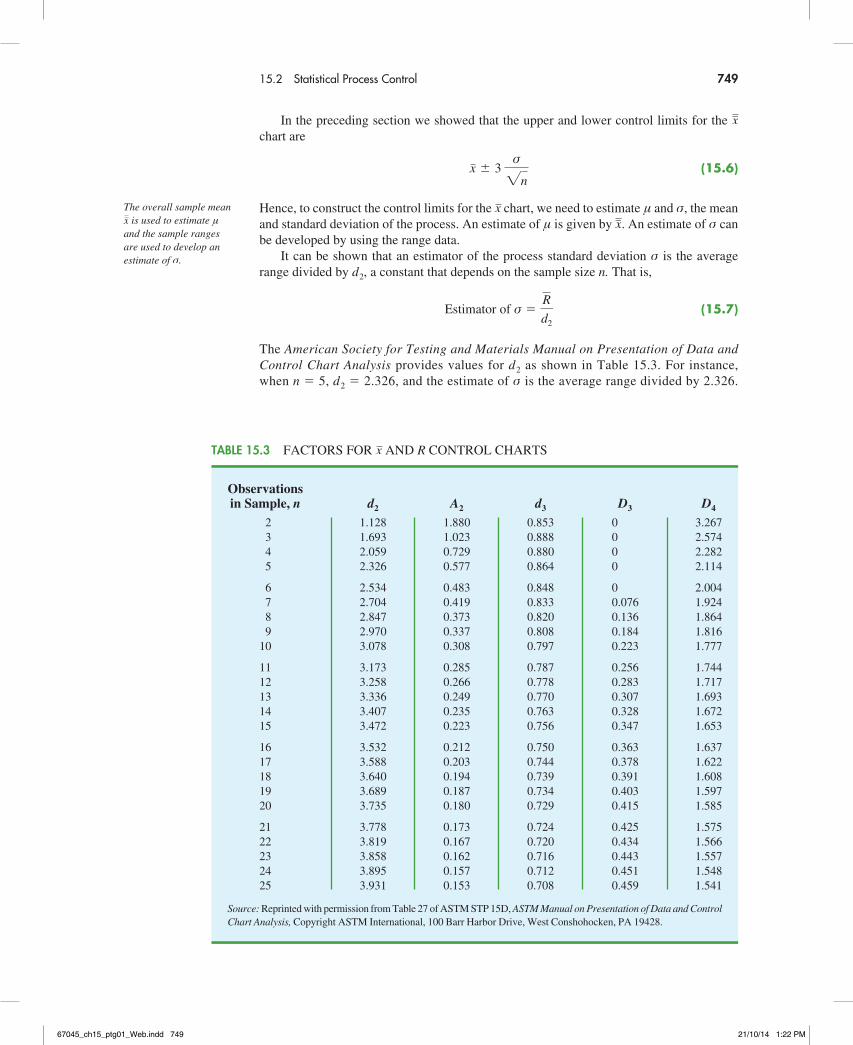
The sampling distribution of p, as presented in Chapter 7, can be used to determine the variation that can be expected in p values for a process that is in control. Recall that the expected value or mean of p is p, the proportion defective when the process is in control. With samples of size n, the formula for the standard deviation of p, called the standard error of the proportion, is

σp 5 Åp(1 2 p)

n (15.16)

We also learned in Chapter 7 that the sampling distribution of p can be approximated by a normal distribution whenever the sample size is large. With p, the sample size can be considered large whenever the following two conditions are satisfied.

np $ 5

n(1 2 p) $ 5

In summary, whenever the sample size is large, the sampling distribution of p can be ap-proximated by a normal distribution with mean p and standard deviation σp. This distribu-tion is shown in figure 15.9.

Control charts that are based on data indicating the presence of a defect or a number of defects are called attributes control charts. A p chart is an at-tributes control chart.

�p 5

p

E( )

p

p(1 2 p)n

p

FIGURE 15.9 SAMPLING DISTRIBUTION Of p

67045_ch15_ptg01_Web.indd 752 21/10/14 1:23 PM


To establish control limits for a p chart, we follow the same procedure we used to estab-lish control limits for an x chart. That is, the limits for the control chart are set at 3 standard deviations, or standard errors, above and below the proportion defective when the process is in control. Thus, we have the following control limits.

CONTROL LIMITS fOR A p CHART

UCL 5 p 1 3σp

LCL 5 p 2 3σp

(15.17)(15.18)

With p 5 .03 and samples of size n 5 200, equation (15.16) shows that the standard error is

σp 5 Å.03(1 2 .03)

2005 .0121

Hence, the control limits are UCL 5 .03 1 3(.0121) 5 .0663 and LCL 5 .03 2 3(.0121) 5 2.0063. Whenever equation (15.18) provides a negative value for LCL, LCL is set equal to zero in the control chart.

figure 15.10 is the p chart for the mail-sorting process. The points plotted show the sample proportion defective found in samples of letters taken from the process. All points are within the control limits, providing no evidence to conclude that the sorting process is out of control.

If the proportion of defective items for a process that is in control is not known, that value is first estimated by using sample data. Suppose, for example, that k different samples, each of size n, are selected from a process that is in control. The fraction or proportion of defective items in each sample is then determined. Treating all the data collected as one large sample, we can compute the proportion of defective items for all the data; that value can then be used to estimate p, the proportion of defective items observed when the process is in control. Note that this estimate of p also enables us to estimate the standard error of the proportion; upper and lower control limits can then be established.

.02

.01

.00

.03

.04

.05

.06

.07UCL 5 .0663

LCL 5 0

Percent DefectiveWhen in Control

5 10 15

Sample Number

Sam

ple

Pro

port

ion

20 25

FIGURE 15.10 p CHART fOR THE PROPORTION DEfECTIVE IN A MAIL-SORTING PROCESS

67045_ch15_ptg01_Web.indd 753 21/10/14 1:23 PM


np ChartAn np chart is a control chart developed for the number of defective items in a sample. In this case, n is the sample size and p is the probability of observing a defective item when the process is in control. Whenever the sample size is large, that is, when np $ 5 and n(1 2 p) $ 5, the distribution of the number of defective items observed in a sample of size n can be approximated by a normal distribution with mean np and standard deviation !np(1 2 p). Thus, for the mail-sorting example, with n 5 200 and p 5 .03, the number of defective items observed in a sample of 200 letters can be approximated by a normal distribu tion with a mean of 200(.03) 5 6 and a standard deviation of !200(.03)(.97) 5 2.4125.

The control limits for an np chart are set at 3 standard deviations above and below the expected number of defective items observed when the process is in control. Thus, we have the following control limits.

CONTROL LIMITS fOR AN np CHART

UCL 5 np 1 3 2np(1 2 p)

LCL 5 np 2 3 2np(1 2 p)

(15.20)(15.19)

for the mail-sorting process example, with p 5 .03 and n 5 200, the control limits are UCL 5 6 1 3(2.4125) 5 13.2375 and LCL 5 6 2 3(2.4125) 5 21.2375. When LCL is negative, LCL is set equal to zero in the control chart. Hence, if the number of letters di-verted to incorrect routes is greater than 13, the process is concluded to be out of control.

The information provided by an np chart is equivalent to the information provided by the p chart; the only difference is that the np chart is a plot of the number of defective items observed, whereas the p chart is a plot of the proportion of defective items observed. Thus, if we were to conclude that a particular process is out of control on the basis of a p chart, the process would also be concluded to be out of control on the basis of an np chart.

Interpretation of Control ChartsThe location and pattern of points in a control chart enable us to determine, with a small probability of error, whether a process is in statistical control. A primary indication that a process may be out of control is a data point outside the control limits, such as point 5 in figure 15.6. finding such a point is statistical evidence that the process is out of control; in such cases, corrective action should be taken as soon as possible.

In addition to points outside the control limits, certain patterns of the points within the control limits can be warning signals of quality control problems. for example, assume that all the data points are within the control limits but that a large number of points are on one side of the center line. This pattern may indicate that an equipment problem, a change in materials, or some other assignable cause of a shift in quality has occurred. Careful investigation of the production process should be undertaken to determine whether quality has changed.

Another pattern to watch for in control charts is a gradual shift, or trend, over time. for example, as tools wear out, the dimensions of machined parts will gradually deviate from their designed levels. Gradual changes in temperature or humidity, general equipment deterioration, dirt buildup, or operator fatigue may also result in a trend pattern in control charts. Six or seven points in a row that indicate either an increasing or decreasing trend should be cause for concern, even if the data points are all within the control limits. When such a pattern occurs, the process should be reviewed for possible changes or shifts in quality. Corrective action to bring the process back into control may be necessary.

even if all points are within the upper and lower control limits, a process may not be in control. trends in the sample data points or un-usually long runs above or below the center line may also indicate out-of-control conditions.

67045_ch15_ptg01_Web.indd 754 21/10/14 1:23 PM


Exercises

Methods 1. A process that is in control has a mean of μ 5 12.5 and a standard deviation of σ 5 .8.

a. Construct the x_ control chart for this process if samples of size 4 are to be used.

b. Repeat part (a) for samples of size 8 and 16.c. What happens to the limits of the control chart as the sample size is increased? Discuss

why this is reasonable.

2. Twenty-five samples, each of size 5, were selected from a process that was in control. The sum of all the data collected was 677.5 pounds.a. What is an estimate of the process mean (in terms of pounds per unit) when the

process is in control?b. Develop the x

_ control chart for this process if samples of size 5 will be used. Assume

that the process standard deviation is .5 when the process is in control, and that the mean of the process is the estimate developed in part (a).

3. Twenty-five samples of 100 items each were inspected when a process was considered to be operating satisfactorily. In the 25 samples, a total of 135 items were found to be defective.a. What is an estimate of the proportion defective when the process is in control?b. What is the standard error of the proportion if samples of size 100 will be used for

statistical process control?c. Compute the upper and lower control limits for the control chart.

4. A process sampled 20 times with a sample of size 8 resulted in x 5 28.5 and R 5 1.6. Compute the upper and lower control limits for the x and R charts for this process.

Applications 5. Temperature is used to measure the output of a production process. When the

process is in control, the mean of the process is μ 5 128.5 and the standard deviation is σ 5 .4.a. Construct the x chart for this process if samples of size 6 are to be used.b. Is the process in control for a sample providing the following data?

128.8 128.2 129.1 128.7 128.4 129.2

c. Is the process in control for a sample providing the following data?

129.3 128.7 128.6 129.2 129.5 129.0

6. A quality control process monitors the weight per carton of laundry detergent. Control limits are set at UCL 5 20.12 ounces and LCL 5 19.90 ounces. Samples of size 5 are used

NOTES AND COMMENTS

1. Because the control limits for the x chart de-pend on the value of the average range, these limits will not have much meaning unless the process variability is in control. In practice, the R chart is usually constructed before the x chart; if the R chart indicates that the pro-cess variability is in control, then the x chart is constructed. The StatTools X/R Charts option

provides the x chart and the R chart simulta-neously. The steps of this procedure are de-scribed in the chapter appendix.

2. An np chart is used to monitor a process in terms of the number of defects. The Motorola Six Sigma Quality Level sets a goal of producing no more than 3.4 defects per million operations; this goal implies p 5 .0000034.

testSELF

67045_ch15_ptg01_Web.indd 755 21/10/14 1:23 PM


for the sampling and inspection process. What are the process mean and process standard deviation for the manufacturing operation?

7. The Goodman Tire and Rubber Company periodically tests its tires for tread wear under simulated road conditions. To study and control the manufacturing process, 20 samples, each containing three radial tires, were chosen from different shifts over several days of operation, with the following results. Assuming that these data were collected when the manufacturing process was believed to be operating in control, develop the R and x charts.

Sample Tread Wear*

1 31 42 28 2 26 18 35 3 25 30 34 4 17 25 21 5 38 29 35 6 41 42 36 7 21 17 29 8 32 26 28 9 41 34 33 10 29 17 30 11 26 31 40 12 23 19 25 13 17 24 32 14 43 35 17 15 18 25 29 16 30 42 31 17 28 36 32 18 40 29 31 19 18 29 28 20 22 34 26

*Hundredths of an inch

�leWEBTires

8. Over several weeks of normal, or in-control, operation, 20 samples of 150 packages each of synthetic-gut tennis strings were tested for breaking strength. A total of 141 packages of the 3000 tested failed to conform to the manufacturer’s specifications.a. What is an estimate of the process proportion defective when the system is in control?b. Compute the upper and lower control limits for a p chart.c. With the results of part (b), what conclusion should be made about the process if tests

on a new sample of 150 packages find 12 defective? Do there appear to be assignable causes in this situation?

d. Compute the upper and lower control limits for an np chart.e. Answer part (c) using the results of part (d).f. Which control chart would be preferred in this situation? Explain.

9. An airline operates a call center to handle customer questions and complaints. The airline monitors a sample of calls to help ensure that the service being provided is of high quality. Ten random samples of 100 calls each were monitored under normal conditions. The center can be thought of as being in control when these 10 samples were taken. The number of calls in each sample not resulting in a satisfactory resolution for the customer is as follows:

4 5 3 2 3 3 4 6 4 7

a. What is an estimate of the proportion of calls not resulting in a satisfactory outcome for the customer when the center is in control?

67045_ch15_ptg01_Web.indd 756 21/10/14 1:23 PM

15.3 Acceptance Sampling 757

Results compared withspeci�ed qualitycharacteristics

Sampleinspected for quality

Sample selected

Lot received

Send to productionor customer

Accept the lot

Decide on dispositionof the lot

Reject the lot

Quality issatisfactory

Quality isnot satisfactory

FIGURE 15.11 ACCEPTANCE SAMPLING PROCEDURE

b. Construct the upper and lower limits for a p chart for the manufacturing process, assuming each sample has 100 calls.

c. With the results of part (b), what conclusion should be made if a sample of 100 has 12 calls not resulting in a satisfactory resolution for the customer?

d. Compute the upper and lower limits for the np chart.e. With the results of part (d), what conclusion should be made if a sample of 100 calls

has 12 not resulting in a satisfactory conclusion for the customer?

15.3 Acceptance SamplingIn acceptance sampling, the items of interest can be incoming shipments of raw materials or pur-chased parts as well as finished goods from final assembly. Suppose we want to decide whether to accept or reject a group of items on the basis of specified quality characteristics. In quality con-trol terminology, the group of items is a lot, and acceptance sampling is a statistical method that enables us to base the accept-reject decision on the inspection of a sample of items from the lot.

The general steps of acceptance sampling are shown in figure 15.11. After a lot is received, a sample of items is selected for inspection. The results of the inspection are com-pared to specified quality characteristics. If the quality characteristics are satisfied, the lot is accepted and sent to production or shipped to customers. If the lot is rejected, managers must decide on its disposition. In some cases, the decision may be to keep the lot and remove the unacceptable or nonconforming items. In other cases, the lot may be returned to the supplier at the supplier’s expense; the extra work and cost placed on the supplier can motivate the

67045_ch15_ptg01_Web.indd 757 21/10/14 1:23 PM


supplier to provide high-quality lots. finally, if the rejected lot consists of finished goods, the goods must be scrapped or reworked to meet acceptable quality standards.

The statistical procedure of acceptance sampling is based on the hypothesis testing method-ology presented in Chapter 9. The null and alternative hypotheses are stated as follows.

H0:

Ha: Good-quality lot

Poor-quality lot

Table 15.4 shows the results of the hypothesis testing procedure. Note that correct deci-sions correspond to accepting a good-quality lot and rejecting a poor-quality lot. However, as with other hypothesis testing procedures, we need to be aware of the possibilities of making a Type I error (rejecting a good-quality lot) or a Type II error (accepting a poor-quality lot).

The probability of a Type I error creates a risk for the producer of the lot and is known as the producer’s risk. for example, a producer’s risk of .05 indicates a 5% chance that a good-quality lot will be erroneously rejected. The probability of a Type II error, on the other hand, creates a risk for the consumer of the lot and is known as the consumer’s risk. for example, a consumer’s risk of .10 means a 10% chance that a poor-quality lot will be er-roneously accepted and thus used in production or shipped to the customer. Specific values for the producer’s risk and the consumer’s risk can be controlled by the person designing the acceptance sampling procedure. To illustrate how to assign risk values, let us consider the problem faced by kALI, Inc.

KALI, Inc.: An Example of Acceptance SamplingkALI, Inc., manufactures home appliances that are marketed under a variety of trade names. However, kALI does not manufacture every component used in its products. Several com-ponents are purchased directly from suppliers. for example, one of the components that kALI purchases for use in home air conditioners is an overload protector, a device that turns off the compressor if it overheats. The compressor can be seriously damaged if the overload protector does not function properly, and therefore kALI is concerned about the quality of the overload protectors. One way to ensure quality would be to test every component received through an approach known as 100% inspection. However, to determine proper functioning of an overload protector, the device must be subjected to time- consuming and expensive tests, and kALI cannot justify testing every overload protector it receives.

Instead, kALI uses an acceptance sampling plan to monitor the quality of the overload protectors. The acceptance sampling plan requires that kALI’s quality control inspectors select and test a sample of overload protectors from each shipment. If very few defective units are found in the sample, the lot is probably of good quality and should be accepted.

Acceptance sampling has the following advantages over 100% inspection:1. Usually less expensive2. Less product damage

due to less handling and testing

3. Fewer inspectors required

4. the only approach possible if destructive testing must be used

State of the Lot

H0 True H0 False Good-Quality Lot Poor-Quality Lot Accept the Lot Correct decision Type II error (accepting a poor-quality lot)Decision

Reject the Lot Type I error Correct decision (rejecting a good-quality lot)

TABLE 15.4 THE OUTCOMES Of ACCEPTANCE SAMPLING

67045_ch15_ptg01_Web.indd 758 21/10/14 1:23 PM


However, if a large number of defective units are found in the sample, the lot is probably of poor quality and should be rejected.

An acceptance sampling plan consists of a sample size n and an acceptance criterion c. The acceptance criterion is the maximum number of defective items that can be found in the sample and still indicate an acceptable lot. for example, for the kALI problem let us assume that a sample of 15 items will be selected from each incoming shipment or lot. furthermore, assume that the manager of quality control states that the lot can be accepted only if no defective items are found. In this case, the acceptance sampling plan established by the quality control manager is n 5 15 and c 5 0.

This acceptance sampling plan is easy for the quality control inspector to implement. The inspector simply selects a sample of 15 items, performs the tests, and reaches a conclu-sion based on the following decision rule.

Accept the lot if zero defective items are found. Reject the lot if one or more defective items are found.

Before implementing this acceptance sampling plan, the quality control manager wants to evaluate the risks or errors possible under the plan. The plan will be implemented only if both the producer’s risk (Type I error) and the consumer’s risk (Type II error) are controlled at reasonable levels.

Computing the Probability of Accepting a LotThe key to analyzing both the producer’s risk and the consumer’s risk is a “what-if” type of analysis. That is, we will assume that a lot has some known percentage of defective items and compute the probability of accepting the lot for a given sampling plan. By varying the assumed percentage of defective items, we can examine the effect of the sampling plan on both types of risks.

Let us begin by assuming that a large shipment of overload protectors has been received and that 5% of the overload protectors in the shipment are defective. for a shipment or lot with 5% of the items defective, what is the probability that the n 5 15, c 5 0 sampling plan will lead us to accept the lot? Because each overload protector tested will be either defective or nondefective and because the lot size is large, the number of defective items in a sample of 15 has a binomial distribution. The binomial probability function, which was presented in Chapter 5, follows.

BINOMIAL PROBABILITy fUNCTION fOR ACCEPTANCE SAMPLING

f (x) 5n!

x!(n 2 x)! px(1 2 p)(n2x) (15.21)

where

n 5

p 5

x 5

f (x) 5

the sample size

the proportion of defective items in the lot

the number of defective items in the sample

the probability of x defective items in the sample

for the kALI acceptance sampling plan, n 5 15; thus, for a lot with 5% defective ( p 5 .05), we have

f(x) 515!

x!(15 2 x)! (.05)x(1 2 .05)(152x) (15.22)

67045_ch15_ptg01_Web.indd 759 21/10/14 1:23 PM


Using equation (15.22), f (0) will provide the probability that zero overload protectors will be defective and the lot will be accepted. In using equation (15.22), recall that 0! 5 1. Thus, the probability computation for f (0) is

f (0) 515!

0!(15 2 0)! (.05)0(1 2 .05)(1520)

515!

0!(15)! (.05)0(.95)15 5 (.95)15 5 .4633

We now know that the n 5 15, c 5 0 sampling plan has a .4633 probability of accepting a lot with 5% defective items. Hence, there must be a corresponding 1 2 .4633 5 .5367 probability of rejecting a lot with 5% defective items.

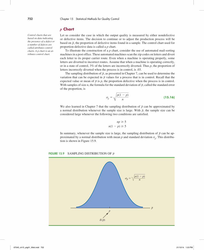
Excel’s BINOM.DIST function can be used to simplify making these binomial prob-ability calculations. Using this function, we can determine that if the lot contains 10% defective items, there is a .2059 probability that the n 5 15, c 5 0 sampling plan will in-dicate an acceptable lot. The probability that the n 5 15, c 5 0 sampling plan will lead to the acceptance of lots with 1%, 2%, 3%, . . . defective items is summarized in Table 15.5.

Using the probabilities in Table 15.5, a graph of the probability of accepting the lot versus the percent defective in the lot can be drawn as shown in figure 15.12. This graph, or curve, is called the operating characteristic (OC) curve for the n 5 15, c 5 0 acceptance sampling plan.

Perhaps we should consider other sampling plans, ones with different sample sizes n or different acceptance criteria c. first consider the case in which the sample size remains n 5 15 but the acceptance criterion increases from c 5 0 to c 5 1. That is, we will now accept the lot if zero or one defective component is found in the sample. for a lot with 5% defective items ( p 5 .05), the binomial probability function in equation (15.21), or Excel’s BINOM.DIST function, can be used to compute f (0) 5 .4633 and f (1) 5 .3658. Thus, there is a .4633 1 .3658 5 .8291 probability that the n 5 15, c 5 1 plan will lead to the acceptance of a lot with 5% defective items.

Continuing these calculations, we obtain figure 15.13, which shows the operating characteristic curves for four alternative acceptance sampling plans for the kALI problem. Samples of size 15 and 20 are considered. Note that regardless of the proportion defective in the lot, the n 5 15, c 5 1 sampling plan provides the highest probabilities of accepting the lot. The n 5 20, c 5 0 sampling plan provides the lowest probabilities of accepting the lot; however, that plan also provides the highest probabilities of rejecting the lot.

Percent Defective in the Lot Probability of Accepting the Lot 1 .8601 2 .7386 3 .6333 4 .5421 5 .4633 10 .2059 15 .0874 20 .0352 25 .0134

TABLE 15.5 PROBABILITy Of ACCEPTING THE LOT fOR THE kALI PROBLEM WITH n 5 15 AND c 5 0

67045_ch15_ptg01_Web.indd 760 21/10/14 1:23 PM


.10

.20

.30

.40

.50

.60

.70

.80

.90

1.00

Pro

babi

lity

of A

ccep

ting

the

Lot

5 10 15 20 250

Percent Defective in the Lot

n 5 20, c 5 1

n 5 15, c 5 1

n 5 20, c 5 0

n 5 15, c 5 0

FIGURE 15.13 OPERATING CHARACTERISTIC CURVES fOR fOUR ACCEPTANCE SAMPLING PLANS

.10

.20

.30

.40

.50

.60

.70

.80

.90

1.00

Pro

babi

lity

of A

ccep

ting

the

Lot

5 10 15 20 250


FIGURE 15.12 OPERATING CHARACTERISTIC CURVE fOR THE n 5 15, c 5 0 ACCEPTANCE SAMPLING PLAN

67045_ch15_ptg01_Web.indd 761 21/10/14 1:23 PM


Selecting an Acceptance Sampling PlanNow that we know how to use the binomial distribution to compute the probability of ac-cepting a lot with a given proportion defective, we are ready to select the values of n and c that determine the desired acceptance sampling plan for the application being studied. To develop this plan, managers must specify two values for the fraction defective in the lot. One value, denoted p0, will be used to control for the producer’s risk, and the other value, denoted p1, will be used to control for the consumer’s risk.

We will use the following notation.

α 5 the producer’s risk; the probability of rejecting a lot with p0 defective items

β 5 the consumer’s risk; the probability of accepting a lot with p1 defective items

Suppose that for the kALI problem, the managers specify that p0 5 .03 and p1 5 .15. from the OC curve for n 5 15, c 5 0 in figure 15.14, we see that p0 5 .03 provides a producer’s risk of approximately 1 2 .63 5 .37, and p1 5 .15 provides a consumer’s risk of approxi-mately .09. Thus, if the managers are willing to tolerate both a .37 probability of rejecting a lot with 3% defective items (producer’s risk) and a .09 probability of accepting a lot with 15% defective items (consumer’s risk), the n 5 15, c 5 0 acceptance sampling plan would be acceptable.

Suppose, however, that the managers request a producer’s risk of α 5 .10 and a consumer’s risk of β 5 .19. We see that now the n 5 15, c 5 0 sampling plan has a better-than-desired consumer’s risk but an unacceptably large producer’s risk. The fact

.10

.20

.30

.40

.50

.60

.70

.80

.90

1.00

Pro

babi

lity

of A

ccep

ting

the

Lot

5 10 15 20 250


(12 )

�

5 Producer’s risk (theprobability of makinga Type I error)

� 5 Consumer’s risk (theprobability of makinga Type II error)

p0 p1

FIGURE 15.14 OPERATING CHARACTERISTIC CURVE fOR n 5 15, c 5 0 WITH p0 5 .03 AND p1 5 .15

67045_ch15_ptg01_Web.indd 762 21/10/14 1:23 PM


that α 5 .37 indicates that 37% of the lots will be erroneously rejected when only 3% of the items in them are defective. The producer’s risk is too high, and a different ac-ceptance sampling plan should be considered.

Using p0 5 .03, α 5 .10, p1 5 .15, and β 5 .20, figure 15.13 shows that the ac ceptance sampling plan with n 5 20 and c 5 1 comes closest to meeting both the producer’s and the consumer’s risk requirements.

As shown in this section, several computations and several operating characteristic curves may need to be considered to determine the sampling plan with the desired producer’s and consumer’s risk. fortunately, tables of sampling plans are published. for example, the American Military Standard Table, MIL-STD-105D, provides information helpful in designing acceptance sampling plans. More advanced texts on quality control, such as those

exercise 13 at the end of this section will ask you to compute the producer’s risk and the consumer’s risk for the n 5 20, c 5 1 sampling plan.

Sample n1

items

Find x1

defective itemsin this sample

Isx1 # c1

?

Acceptthe lot

Isx1 $ c2

?

Rejectthe lot

Sample n2

additional items

Find x2

defective itemsin this sample

Isx1 1 x2 # c3

?

Yes

Yes

YesNo

No

No

FIGURE 15.15 A TWO-STAGE ACCEPTANCE SAMPLING PLAN

67045_ch15_ptg01_Web.indd 763 21/10/14 1:23 PM


listed in the bibliography, describe the use of such tables. The advanced texts also discuss the role of sampling costs in determining the optimal sampling plan.

Multiple Sampling PlansThe acceptance sampling procedure we presented for the kALI problem is a single-sample plan. It is called a single-sample plan because only one sample or sampling stage is used. After the number of defective components in the sample is determined, a deci-sion must be made to accept or reject the lot. An alternative to the single-sample plan is a multiple sampling plan, in which two or more stages of sampling are used. At each stage a decision is made among three possibilities: stop sampling and accept the lot, stop sampling and reject the lot, or continue sampling. Although they are more complex than single-sample plans, multiple sampling plans often result in a smaller total sample size than single-sample plans with the same α and β probabilities.

The logic of a two-stage, or double-sample, plan is shown in figure 15.15. Initially a sample of n1 items is selected. If the number of defective components x1 is less than or equal to c1, accept the lot. If x1 is greater than or equal to c2, reject the lot. If x1 is between c1 and c2 (c1 , x1 , c2), select a second sample of n2 items. Determine the combined, or total, number of defective components from the first sample (x1) and the second sample (x2). If x1 1 x2 # c3, accept the lot; otherwise reject the lot. The develop-ment of the double-sample plan is more difficult because the sample sizes n1 and n2 and the acceptance numbers c1, c2, and c3 must meet both the producer’s and consumer’s risks desired.

NOTES AND COMMENTS

1. The use of the binomial distribution for ac-ceptance sampling is based on the assumption of large lots. If the lot size is small, the hyper-geometric distribution is appropriate.

2. In the MIL-STD-105D sampling tables, p0 is called the acceptable quality level (AQL). In some sampling tables, p1 is called the lot toler-ance percent defective (LTPD) or the rejectable quality level (RQL). Many of the published sampling plans also use quality indexes such as the indifference quality level (IQL) and the average outgoing quality limit (AOQL). The more advanced texts listed in the bibliography

provide a complete discussion of these other indexes.

3. In this section we provided an introduction to attributes sampling plans. In these plans each item sampled is classified as nondefective or defective. In variables sampling plans, a sample is taken and a measurement of the quality char-acteristic is taken. for example, for gold jewelry a measurement of quality may be the amount of gold it contains. A simple statistic such as the average amount of gold in the sample jewelry is computed and compared with an allowable value to determine whether to accept or reject the lot.

Exercises

Methods10. for an acceptance sampling plan with n 5 25 and c 5 0, find the probability of accepting

a lot that has a defect rate of 2%. What is the probability of accepting the lot if the defect rate is 6%?

11. Consider an acceptance sampling plan with n 5 20 and c 5 0. Compute the producer’s risk for each of the following cases.a. The lot has a defect rate of 2%.b. The lot has a defect rate of 6%.

testSELF

67045_ch15_ptg01_Web.indd 764 21/10/14 1:23 PM

Glossary 765

12. Repeat exercise 11 for the acceptance sampling plan with n 5 20 and c 5 1. What happens to the producer’s risk as the acceptance number c is increased? Explain.

Applications13. Refer to the kALI problem presented in this section. The quality control manager requested

a producer’s risk of .10 when p0 was .03 and a consumer’s risk of .20 when p1 was .15. Consider the acceptance sampling plan based on a sample size of 20 and an acceptance number of 1. Answer the following questions.a. What is the producer’s risk for the n 5 20, c 5 1 sampling plan?b. What is the consumer’s risk for the n 5 20, c 5 1 sampling plan?c. Does the n 5 20, c 5 1 sampling plan satisfy the risks requested by the quality control

manager? Discuss.

14. To inspect incoming shipments of raw materials, a manufacturer is considering samples of sizes 10, 15, and 19. Select a sampling plan that provides a producer’s risk of α 5 .03 when p0 is .05 and a consumer’s risk of β 5 .12 when p1 is .30.

15. A domestic manufacturer of watches purchases quartz crystals from a Swiss firm. The crystals are shipped in lots of 1000. The acceptance sampling procedure uses 20 randomly selected crystals.a. Construct operating characteristic curves for acceptance numbers of 0, 1, and 2.b. If p0 is .01 and p1 5 .08, what are the producer’s and consumer’s risks for each sam-

pling plan in part (a)?

Summary

In this chapter we discussed how statistical methods can be used to assist in the control of quality. We first presented the x, R, p, and np control charts as graphical aids in monitoring process quality. Control limits are established for each chart; samples are selected periodi-cally, and the data points plotted on the control chart. Data points outside the control limits indicate that the process is out of control and that corrective action should be taken. Patterns of data points within the control limits can also indicate potential quality control problems and suggest that corrective action may be warranted.

We also considered the technique known as acceptance sampling. With this procedure, a sample is selected and inspected. The number of defective items in the sample provides the basis for accepting or rejecting the lot. The sample size and the acceptance criterion can be adjusted to control both the producer’s risk (Type I error) and the consumer’s risk (Type II error).

Glossary

Total quality (TQ) A total system approach to improving customer satisfaction and lower-ing real cost through a strategy of continuous improvement and learning.Six Sigma A methodology that uses measurement and statistical analysis to achieve a level of quality so good that for every million opportunities no more than 3.4 defects will occur.Quality control A series of inspections and measurements that determine whether quality standards are being met.Assignable causes Variations in process outputs that are due to factors such as machine tools wearing out, incorrect machine settings, poor-quality raw materials, operator error,

67045_ch15_ptg01_Web.indd 765 21/10/14 1:23 PM


and so on. Corrective action should be taken when assignable causes of output variation are detected.Common causes Normal or natural variations in process outputs that are due purely to chance. No corrective action is necessary when output variations are due to common causes.Control chart A graphical tool used to help determine whether a process is in control or out of control.x chart A control chart used when the quality of the output of a process is measured in terms of the mean value of a variable such as a length, weight, temperature, and so on.R chart A control chart used when the quality of the output of a process is measured in terms of the range of a variable.p chart A control chart used when the quality of the output of a process is measured in terms of the proportion defective.np chart A control chart used to monitor the quality of the output of a process in terms of the number of defective items.Lot A group of items such as incoming shipments of raw materials or purchased parts as well as finished goods from final assembly.Acceptance sampling A statistical method in which the number of defective items found in a sample is used to determine whether a lot should be accepted or rejected.Producer’s risk The risk of rejecting a good-quality lot; a Type I error.Consumer’s risk The risk of accepting a poor-quality lot; a Type II error.Acceptance criterion The maximum number of defective items that can be found in the sample and still indicate an acceptable lot.Operating characteristic (OC) curve A graph showing the probability of accepting the lot as a function of the percentage defective in the lot. This curve can be used to help de-termine whether a particular acceptance sampling plan meets both the producer’s and the consumer’s risk requirements.Multiple sampling plan A form of acceptance sampling in which more than one sample or stage is used. On the basis of the number of defective items found in a sample, a decision will be made to accept the lot, reject the lot, or continue sampling.

Key Formulas

Standard Error of the Mean

σx 5σ!n

(15.1)

Control Limits for an x Chart: Process Mean and Standard Deviation Known

UCL 5

LCL 5

μ 1 3σx

μ 2 3σx

Overall Sample Mean

x 5x1 1 x

2 1 c1 xk

k (15.4)

Average Range

R 5R1 1 R

2 1 c1 Rk

k (15.5)

(15.2)(15.3)

67045_ch15_ptg01_Web.indd 766 21/10/14 1:23 PM

Supplementary Exercises 767

Control Limits for an x Chart: Process Mean and Standard Deviation Unknown

x 6 A2R (15.8)

Control Limits for an R Chart

UCL 5 R D4 (15.14)

LCL 5 R D3 (15.15)

Standard Error of the Proportion

σp 5 Åp(1 2 p)

n (15.16)

Control Limits for a p Chart

UCL 5 p 1 3σp

LCL 5 p 2 3σp

Control Limits for an np Chart

UCL 5 np 1 3 2np(1 2 p)

LCL 5 np 2 3 2np(1 2 p)

Binomial Probability Function for Acceptance Sampling

f (x) 5n!

x!(n 2 x)! px(1 2 p)(n2x) (15.21)

Supplementary Exercises

16. Samples of size 5 provided the following 20 sample means for a production process that is believed to be in control.

95.72 95.24 95.1895.44 95.46 95.3295.40 95.44 95.0895.50 95.80 95.2295.56 95.22 95.0495.72 94.82 95.4695.60 95.78

a. Based on these data, what is an estimate of the mean when the process is in control?b. Assume that the process standard deviation is σ 5 .50. Develop the x

_ control chart for

this production process. Assume that the mean of the process is the estimate developed in part (a).

c. Do any of the 20 sample means indicate that the process was out of control?

17. Product filling weights are normally distributed with a mean of 350 grams and a standard deviation of 15 grams.a. Develop the control limits for the x

_ chart for samples of size 10, 20, and 30.

b. What happens to the control limits as the sample size is increased?

(15.17)(15.18)

(15.19)(15.20)

67045_ch15_ptg01_Web.indd 767 21/10/14 1:23 PM


c. What happens when a Type I error is made?d. What happens when a Type II error is made?e. What is the probability of a Type I error for samples of size 10, 20, and 30?f. What is the advantage of increasing the sample size for control chart purposes? What

error probability is reduced as the sample size is increased?

18. Twenty-five samples of size 5 resulted in x 5 5.42 and R 5 2.0. Compute control limits for the x and R charts, and estimate the standard deviation of the process.

19. The following are quality control data for a manufacturing process at kensport Chemical Company. The data show the temperature in degrees centigrade at five points in time dur-ing a manufacturing cycle. The company is interested in using control charts to monitor the temperature of its manufacturing process. Construct the x chart and R chart. What conclusions can be made about the quality of the process?

Sample x R Sample x R

1 95.72 1.0 11 95.80 .6 2 95.24 .9 12 95.22 .2 3 95.18 .8 13 95.56 1.3 4 95.44 .4 14 95.22 .5 5 95.46 .5 15 95.04 .8 6 95.32 1.1 16 95.72 1.1 7 95.40 .9 17 94.82 .6 8 95.44 .3 18 95.46 .5 9 95.08 .2 19 95.60 .4 10 95.50 .6 20 95.74 .6

Observations

Sample 1 2 3 4 5

1 3.05 3.08 3.07 3.11 3.11 2 3.13 3.07 3.05 3.10 3.10 3 3.06 3.04 3.12 3.11 3.10 4 3.09 3.08 3.09 3.09 3.07 5 3.10 3.06 3.06 3.07 3.08 6 3.08 3.10 3.13 3.03 3.06 7 3.06 3.06 3.08 3.10 3.08 8 3.11 3.08 3.07 3.07 3.07 9 3.09 3.09 3.08 3.07 3.09 10 3.06 3.11 3.07 3.09 3.07

�leWEBCoffee

20. The following data were collected for the Master Blend Coffee production process. The data show the filling weights based on samples of 3-pound cans of coffee. Use these data to construct the x and R charts. What conclusions can be made about the quality of the production process?

67045_ch15_ptg01_Web.indd 768 21/10/14 1:23 PM

Appendix Control Charts Using StatTools 769

21. An insurance company samples claim forms for errors created by its employees as well as the amount of time it takes to process a claim.a. When the process is in control, the proportion of claims with an error is .033. A p chart

has LCL 5 0 and UCL 5 .068. Plot the following seven sample results: .035, .062, .055, .049, .058, .066, and .055. Comment on whether there might be concern about the quality of the process.

b. An x chart for the mean processing time has LCL 5 22.2 and UCL 5 24.5. The mean is μ 5 23.35 when the claim process is in control. Plot the following seven sample results: 22.4, 22.6, 22.65, 23.2, 23.4, 23.85, and 24.1. Comment on whether there might be concern about the quality of the process.

22. Managers of 1200 different retail outlets make twice-a-month restocking orders from a central warehouse. Past experience shows that 4% of the orders result in one or more errors such as wrong item shipped, wrong quantity shipped, and item requested but not shipped. Random samples of 200 orders are selected monthly and checked for accuracy.a. Construct a control chart for this situation.b. Six months of data show the following numbers of orders with one or more errors: 10,

15, 6, 13, 8, and 17. Plot the data on the control chart. What does your plot indicate about the order process?

23. An n 5 10, c 5 2 acceptance sampling plan is being considered; assume that p0 5 .05 and p1 5 .20.a. Compute both producer’s and consumer’s risk for this acceptance sampling plan.b. Would the producer, the consumer, or both be unhappy with the proposed sam-

pling plan?c. What change in the sampling plan, if any, would you recommend?

24. An acceptance sampling plan with n 5 15 and c 5 1 has been designed with a producer’s risk of .075.a. Was the value of p0 .01, .02, .03, .04, or .05? What does this value mean?b. What is the consumer’s risk associated with this plan if p1 is .25?

25. A manufacturer produces lots of a canned food product. Let p denote the proportion of the lots that do not meet the product quality specifications. An n 5 25, c 5 0 acceptance sampling plan will be used.a. Compute points on the operating characteristic curve when p 5 .01, .03, .10, and .20.b. Plot the operating characteristic curve.c. What is the probability that the acceptance sampling plan will reject a lot containing

.01 defective products?

Appendix Control Charts Using StatToolsIn this appendix we show how StatTools can be used to construct an x chart and an R chart for the Jensen Computer Supplies data shown in Table 15.2. figure 15.16 is an Excel worksheet containing the Jensen data with the StatTools - Xbar and R Control Charts dialog box in the foreground. Begin by using the Data Set Manager to create a StatTools data set for these data using the procedure described in the appendix in Chapter 1. The following steps describe how StatTools can be used to provide both control charts.

Step 1. Click the StatTools tab on the RibbonStep 2. In the Analyses group, click Quality ControlStep 3. Choose the X/R Charts option

�leWEBJensen

67045_ch15_ptg01_Web.indd 769 21/10/14 1:23 PM


Step 4. When the StatTools - Xbar and R Control Charts dialog box appears (figure 15.16): Select X-Bar/R Chart in the Chart Type box In the Variables section, select Observation 1, Observation 2, Observation 3, Observation 4, and Observation 5Click OK

An x chart similar to the one in figure 15.7 will appear. It will be followed by an R chart similar to the one in figure 15.8.

FIGURE 15.16 EXCEL WORkSHEET fOR JENSEN COMPUTER SUPPLIES

67045_ch15_ptg01_Web.indd 770 21/10/14 1:23 PM

Documents

Statistical Methods for Quality Control - Cengage Methods for Quality Control CONTENTS STATISTICS IN PRACTICE: DOW CHEMICAL COMPANy 15.1 PHILOSOPHIES AND fRAMEWORkS …