Embed Size (px)
Citation preview
Unpublished Exercises
Statistical Mechanics: Entropy, OrderParameters, and Complexity
James P. SethnaLaboratory of Atomic and Solid State Physics, Cornell University, Ithaca, NY
14853-2501
The author provides this version of this manuscript with the primary in-tention of making the text accessible electronically—through web searchesand for browsing and study on computers. Oxford University Press retainsownership of the copyright. Hard-copy printing, in particular, is subject tothe same copyright rules as they would be for a printed book.
CLARENDON PRESS . OXFORD
2010


Contents
Contents v
List of figures vii
N Unpublished Exercises 1
Exercises 1N.1 The Greenhouse effect and cooling coffee 1N.2 The Dyson sphere 2N.3 Biggest of bunch: Gumbel 3N.4 First to fail: Weibull 4N.5 Random energy model 6N.6 A fair split? Number partitioning 7N.7 Fracture nucleation: elastic theory has zero radius
of convergence 10N.8 Extreme value statistics: Gumbel, Weibull, and
Frechet 13N.9 Cardiac dynamics 14N.10 Quantum dissipation from phonons 16N.11 The Gutenberg Richter law 17N.12 Random Walks 17N.13 Period Doubling 18N.14 Hysteresis and Barkhausen Noise 19N.15 Variational mean-field derivation 20N.16 Avalanche Size Distribution 20N.17 Ising Lower Critical Dimension 21N.18 XY Lower Critical Dimension and the Mermin-
Wagner Theorem 22N.19 Long-range Ising 22N.20 Equilibrium Crystal Shapes 22N.21 Condition Number and Accuracy 24N.22 Sherman–Morrison formula 24N.23 Methods of interpolation 25N.24 Numerical definite integrals 25N.25 Numerical derivatives 27N.26 Summing series 27N.27 Random histograms 27N.28 Monte Carlo integration 27N.29 The Birthday Problem 28N.30 Washboard Potential 29

vi Contents
N.31 Sloppy Minimization 29N.32 Sloppy Monomials 30N.33 Conservative differential equations: Accuracy and
fidelity 31
References 35

List of figures
N.1 Stretched block 10L/L = F/(YA)∆
MaterialElastic
N.2 Fractured block 10MaterialElastic
Aγ2Surface Energy
N.3 Critical crack 11P < 0
Crack length
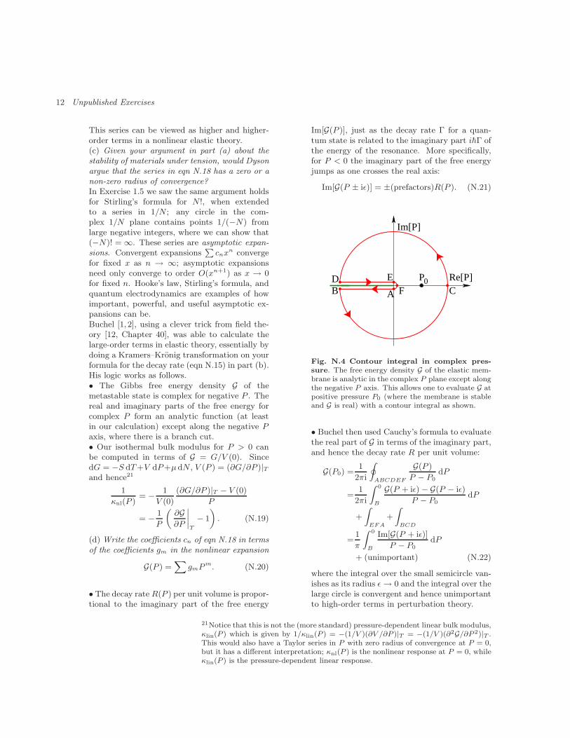
N.4 Contour integral in complex pressure 12 PCFRe[P]
Im[P]
A
EBD 0
N.5 Atomic tunneling from a tip 17 Vo
Qo
AFM /STM tip AFM /STM tip
Substrate Substrate
N.6 Gutenberg Richter Law 174 5 6 7 8
Magnitude1
10
100
1000
10000
Num
ber
of e
arth
quak
es
0.0001 0.01 0.1 1.0 10.0Energy radiated (10
15 joules)
S -2/3
N.7 Random walk scaling 18N.8 Scaling in the period doubling bifurcation diagram 18 δ
α
N.9 Avalanche size distribution 1910
010
210
410
6
Avalanche size S
10-15
10-10
10-5
100
105
Din
t(S,R
)
0.0 0.5 1.0 1.5S
σr
0.1
0.2
Sτ +
σβδ D
int(S
σ r)
R = 4R = 2.25
N.10 Interpolation methods 26interpolation
-π 0 πx
-1
0
1
Firs
t der
ivat
ive
ABCD
-π 0 πx
-1
0
1
Seco
nd d
eriv
ativ
e
ABCD
-π 0 πx
-0.4
-0.2
0
0.2
0.4
Err
or
ABCD
-π 0 πx
-1
0
1
sin(
x) a
ppro
x
ABCD
-π 0 πx
-1
0
1
Firs
t der
ivat
ive
ABCD
1 1.10.4
0.5
-π 0 πx
-1
0
1
Seco
nd D
eriv
ativ
e
ABCD
-π 0 πx
-0.05
0
0.05
Err
or
ABCD
Five data points Ten data points
Interpolatedsin(x)
Firstderivative
Secondderivative
Errorsin(x) −
-π 0 πx
-1
0
1
sin(
x) a
ppro
x
ABCD
Unpublished Exercises N
Exercises
These exercises will likely be included in alater edition of the text, Statistical Mechan-ics: Entropy, Order Parameters, and Complex-ity, by James P. Sethna (Oxford University Press,http://www.physics.cornell.edu/sethna/StatMech).
(N.1) The Greenhouse effect and cooling coffee.
(Astrophysics, Ecology) ©2Vacuum is an excellent insulator. This is whythe surface of the Sun can remain hot (TS =6000 K) even though it faces directly onto outerspace at the microwave background radiationtemperature TMB = 2.725 K, (Exercise 7.15).The main way1 in which heat energy can passthrough vacuum is by thermal electromagneticradiation (photons). We will see in Exercise 7.7that a black body radiates an energy σT 4 persquare meter per second, where σ = 5.67 ×10⁻⁸ J/(s m2 K4).
A vacuum flask or Thermos bottleTM
keeps cof-fee warm by containing the coffee in a Dewar—adouble-walled glass bottle with vacuum betweenthe two walls.(a) Coffee at an initial temperature TH(0) =100 C of volume V = 150 mL is stored in a vac-uum flask with surface area A = 0.1 m2 in a roomof temperature TC = 20 C. Write down symbol-ically the differential equation determining howthe difference between the coffee temperature andthe room temperature ∆(t) = TH(t) − TC de-creases with time, assuming the vacuum surfacesof the dewar are black and remain at the cur-rent temperatures of the coffee and room. Solvethis equation symbolically in the approximation
that ∆ is small compared to Tc (by approximat-ing T 4
H = (TC +∆)4 ≈ T 4C +4∆T 3
C). What is theexponential decay time (the time it take for thecoffee to cool by a factor of e), both symbolicallyand numerically in seconds? (Useful conversion:0 C = 273.15 K.)Real Dewars are not painted black! They arecoated with shiny metals in order to minimizethis radiative heat loss. (White or shiny materi-als not only absorb less radiation, but they alsoemit less radiation, see exercise 7.7.)The outward solar energy flux at the Earth’s or-bit is ΦS = 1370 W/m2, and the Earth’s radiusis approximately 6400 km, rE = 6.4 × 10⁶ m.The Earth reflects about 30% of the radiationfrom the Sun directly back into space (its albedoα ≈ 0.3). The remainder of the energy is even-tually turned into heat, and radiated into spaceagain. Like the Sun and the Universe, the Earthis fairly well described as a black-body radia-tion source in the infrared. We will see in Ex-ercise 7.7 that a black body radiates an en-ergy σT 4 per square meter per second, whereσ = 5.67 × 10⁻⁸ J/(s m2 K4).(b) What temperature TA does the Earth radi-ate at, in order to balance the energy flow fromthe Sun after direct reflection is accounted for?Is that hotter or colder than you would estimatefrom the temperatures you’ve experienced on theEarth’s surface? (Warning: The energy flow in isproportional to the Earth’s cross-sectional area,while the energy flow out is proportional to itssurface area.)
1The sun and stars can also radiate energy by emitting neutrinos. This is particularlyimportant during a supernova.
2 Unpublished Exercises
The reason the Earth is warmer than would beexpected from a simple radiative energy balanceis the greenhouse effect.2 The Earth’s atmo-sphere is opaque in most of the infrared regionin which the Earth’s surface radiates heat. (Thisfrequency range coincides with the vibration fre-quencies of molecules in the Earth’s upper atmo-sphere. Light is absorbed to create vibrations,collisions can exchange vibrational and transla-tional (heat) energy, and the vibrations can lateragain emit light.) Thus it is the Earth’s atmo-sphere which radiates at the temperature TA youcalculated in part (b); the upper atmosphere hasa temperature intermediate between that of theEarth’s surface and interstellar space.The vibrations of oxygen and nitrogen, the maincomponents of the atmosphere, are too symmet-ric to absorb energy (the transitions have nodipole moment), so the main greenhouse gasesare water, carbon dioxide, methane, nitrous ox-ide, and chlorofluorocarbons (CFCs). The lastfour have significantly increased due to humanactivities; CO2 by ∼ 30% (due to burning offossil fuels and clearing of vegetation), CH4 by∼ 150% (due to cattle, sheep, rice farming, es-cape of natural gas, and decomposing garbage),N2O by ∼ 15% (from burning vegetation, in-dustrial emission, and nitrogen fertilizers), andCFCs from an initial value near zero (from for-mer aerosol sprays, now banned to spare theozone layer). Were it not for the Greenhouseeffect, we’d all freeze (like Mars)—but we couldoverdo it, and become like Venus (whose deepand CO2-rich atmosphere leads to a surface tem-perature hot enough to melt lead).
(N.2) The Dyson sphere. (Astrophysics) ©2Life on Earth can be viewed as a heat engine,taking energy a hot bath (the Sun at temper-ature TS = 6000 K) and depositing it into acold bath (interstellar space, at a microwavebackground temperature TMB = 2.725 K, Ex-ercise 7.15). The outward solar energy flux atthe Earth’s orbit is ΦS = 1370 W/m2, and theEarth’s radius is approximately 6400 km, rE =6.4 × 10⁶ m.(a) If life on Earth were perfectly efficient (aCarnot cycle with a hot bath at TS and a cold
bath at TMB), how much useful work (in watts)could be extracted from this energy flow? Com-pare that to the estimated world marketed energyconsumption of 4.5 × 10²⁰ J/year. (Useful con-stant: There are about π × 107 s in a year.)Your answer to part (a) suggests that we havesome ways to go before we run out of solar en-ergy. But let’s think big.(b) If we built a sphere enclosing the Sun at aradius equal to Earth’s orbit (about 150 millionkilometers, RES ≈ 1.5 × 10¹¹ m), by what factorwould the useful work available to our civilizationincrease?This huge construction project is called a Dysonsphere, after the physicist who suggested [4] thatwe look for advanced civilizations by watchingfor large sources of infrared radiation.Earth, however, does not radiate at the temper-ature of interstellar space. It radiates roughly asa black body at near TE = 300 K = 23 C (see,however, Exercise N.1).(c) How much less effective are we at extractingwork from the solar flux, if our heat must be ra-diated effectively to a 300 K cold bath insteadof one at TMB, assuming in both cases we runCarnot engines?There is an alternative point of view, though,which tracks entropy rather than energy. Livingbeings maintain and multiply their low-entropystates by dumping the entropy generated intothe energy stream leading from the Sun to inter-stellar space. New memory storage also intrinsi-cally involves entropy generation (Exercise 5.2);as we move into the information age, we mayeventually care more about dumping entropythan about generating work. In analogy to the‘work effectiveness’ of part (c) (ratio of actualwork to the Carnot upper bound on the work,given the hot and cold baths), we can estimatean entropy-dumping effectiveness (the ratio ofthe actual entropy added to the energy stream,compared to the entropy that could be conceiv-ably added given the same hot and cold baths).(d) How much entropy impinges on the Earthfrom the Sun, per second per square meter cross-sectional area? How much leaves the Earth, persecond per cross-sectional square meter, whenthe solar energy flux is radiated away at tem-
2The glass in greenhouses also is transparent in the visible and opaque in the in-frared. This, it turns out, isn’t why it gets warm inside; the main insulating effectof the glass is to forbid the warm air from escaping. The greenhouse effect is in thatsense poorly named.
Exercises 3
perature TE = 300 K? By what factor f is theentropy dumped to outer space less than the en-tropy we could dump into a heat bath at TMB?From an entropy-dumping standpoint, which ismore important, the hot-bath temperature TS orthe cold-bath temperature (TE or TMB, respec-tively)?For generating useful work, the Sun is the keyand the night sky is hardly significant. Fordumping the entropy generated by civilization,though, the night sky is the giver of life and therealm of opportunity. These two perspectives arenot really at odds. For some purposes, a givenamount of work energy is much more useful atlow temperatures. Dyson later speculated abouthow life could make efficient use of this by run-ning at much colder tempeartures (Exercise 5.1).A hyper-advanced information-based civilizationwould hence want not to radiate in the infrared,but in the microwave range.To do this, it needs to increase the area of theDyson sphere; a bigger sphere can re-radiate theSolar energy flow as black-body radiation at alower temperature. Interstellar space is a goodinsulator, and one can only shove so much heatenergy through it to get to the Universal coldbath. A body at temperature T radiates thelargest possible energy if it is completely black.We will see in Exercise 7.7 that a black body ra-diates an energy σT 4 per square meter per sec-ond, where σ = 5.67 × 10⁻⁸ J/(sm2 K4) is theStefan–Boltzmann constant.(e) How large a radius RD must the Dysonsphere have to achieve 50% entropy-dumping ef-fectiveness? How does this radius compare to thedistance to Pluto (RPS ≈ 6 × 10¹² m)? If wemeasure entropy in bits (using kS = (1/ log 2)instead of kB = 1.3807 × 10⁻²³ J/K), howmany bits per second of entropy can our hyper-advanced civilization dispose of? (You may ig-nore the relatively small entropy impinging fromthe Sun onto the Dyson sphere, and ignore boththe energy and the entropy from outer space.)The sun wouldn’t be bright enough to read byat that distance, but if we had a well-insulatedsphere we could keep it warm inside—only theoutside need be cold. Alternatively, we couldjust build the sphere for our computers, andlive closer in to the Sun; our re-radiated energywould be almost as useful as the original solarenergy.
(N.3) Biggest of bunch: Gumbel. (Mathematics,Statistics, Engineering) ©3Much of statistical mechanics focuses on theaverage behavior in an ensemble, or the meansquare fluctuations about that average. In manycases, however, we are far more interested in theextremes of a distribution.Engineers planning dike systems are interestedin the highest flood level likely in the next hun-dred years. Let the high water mark in yearj be Hj . Ignoring long-term weather changes(like global warming) and year-to-year correla-tions, let us assume that each Hj is an inde-pendent and identically distributed (IID) ran-dom variable with probability density ρ1(Hj).The cumulative distribution function (cdf) is theprobability that a random variable is less than agiven threshold. Let the cdf for a single year beF1(H) = P (H ′ < H) =
R Hρ1(H
′) dH ′.(a) Write the probability FN (H) that the high-est flood level (largest of the high-water marks)in the next N = 1000 years will be less than H,in terms of the probability F1(H) that the high-water mark in a single year is less than H.The distribution of the largest or smallest of Nrandom numbers is described by extreme valuestatistics [10]. Extreme value statistics is avaluable tool in engineering (reliability, disasterpreparation), in the insurance business, and re-cently in bioinformatics (where it is used to de-termine whether the best alignments of an un-known gene to known genes in other organismsare significantly better than that one would gen-erate randomly).(b) Suppose that ρ1(H) = exp(−H/H0)/H0 de-cays as a simple exponential (H > 0). Using theformula
(1 − A) ≈ exp(−A) small A (N.1)
show that the cumulative distribution functionFN for the highest flood after N years is
FN (H) ≈ exp
»
− exp
„
µ − H
β
«–
. (N.2)
for large H. (Why is the probability FN(H)small when H is not large, at large N?) Whatare µ and β for this case?The constants β and µ just shift the scale andzero of the ruler used to measure the variable ofinterest. Thus, using a suitable ruler, the largest
4 Unpublished Exercises
of many events is given by a Gumbel distribution
F (x) = exp(− exp(−x))
ρ(x) = ∂F/∂x = exp(−(x + exp(−x))).(N.3)
How much does the probability distribution forthe largest of N IID random variables depend onthe probability density of the individual randomvariables? Surprisingly little! It turns out thatthe largest of N Gaussian random variables alsohas the same Gumbel form that we found forexponentials. Indeed, any probability distribu-tion that has unbounded possible values for thevariable, but that decays faster than any powerlaw, will have extreme value statistics governedby the Gumbel distribution [5, section 8.3]. Inparticular, suppose
F1(H) ≈ 1 − A exp(−BHδ) (N.4)
as H → ∞ for some positive constants A, B,and δ. It is in the region near H∗[N ], definedby F1(H
∗[N ]) = 1 − 1/N , that FN varies in aninteresting range (because of eqn N.1).(c) Show that the extreme value statisticsFN (H) for this distribution is of the Gumbelform (eqn N.2) with µ = H∗[N ] and β =1/(Bδ H∗[N ]δ−1). (Hint: Taylor expand F1(H)at H∗ to first order.)The Gumbel distribution is universal. It de-scribes the extreme values for any unboundeddistribution whose tails decay faster than apower law.3 (This is quite analogous to the cen-tral limit theorem, which shows that the normalor Gaussian distribution is the universal form forsums of large numbers of IID random variables,so long as the individual random variables havenon-infinite variance.)The Gaussian or standard normal distributionρ1(H) = (1/
√2π) exp(−H2/2), for example, has
a cumulative distribution F1(H) = (1/2)(1 +erf(H/
√2)) which at large H has asymptotic
form F1(H) ∼ 1− (1/√
2πH) exp(−H2/2). Thisis of the general form of eqn N.4 with B = 1/2 andδ = 2, except that A is a slowly varying functionof H . This slow variation does not change theasymptotics. Hints for the numerics are available
in the computer exercises section of the text Website [8].(d) Generate M = 10000 lists of N = 1000random numbers distributed with this Gaussianprobability distribution. Plot a normalized his-togram of the largest entries in each list. Plotalso the predicted form ρN(H) = dFN/dH frompart (c). (Hint: H∗(N) ≈ 3.09023 for N = 1000;check this if it is convenient.)Other types of distributions can have extremevalue statistics in different universality classes(see Exercise N.8). Distributions with power-law tails (like the distributions of earthquakesand avalanches described in Chapter 12) haveextreme value statistics described by Frechet dis-tributions. Distributions that have a strict upperor lower bound4 have extreme value distributionsthat are described by Weibull statistics (see Ex-ercise N.4).
(N.4) First to fail: Weibull.5 (Mathematics,Statistics, Engineering) ©3Suppose you have a brand-new supercomputerwith N = 1000 processors. Your parallelizedcode, which uses all the processors, cannot berestarted in mid-stream. How long a time t canyou expect to run your code before the first pro-cessor fails?This is example of extreme value statistics (seealso exercises N.3 and N.8), where here we arelooking for the smallest value of N random vari-ables that are all bounded below by zero. Forlarge N the probability distribution ρ(t) and sur-vival probability S(t) =
R ∞
tρ(t′) dt′ are often
given by the Weibull distribution
S(t) = e−(t/α)γ
,
ρ(t) =dS
dt= − γ
α
„
t
α
«γ−1
e−(t/α)γ
.(N.5)
Let us begin by assuming that the processorshave a constant rate Γ of failure, so the prob-ability density of a single processor failing attime t is ρ1(t) = Γ exp(−Γt) as t → 0), andthe survival probability for a single processorS1(t) = 1−
R t
0ρ1(t
′)dt′ ≈ 1−Γt for short times.(a) Using (1 − ǫ) ≈ exp(−ǫ) for small ǫ, showthat the the probability SN (t) at time t that all
3The Gumbel distribution can also describe extreme values for a bounded distribu-tion, if the probability density at the boundary goes to zero faster than a powerlaw [10, section 8.2].4More specifically, bounded distributions that have power-law asymptotics haveWeibull statistics; see note 3 and Exercise N.4, part (d).5Developed with the assistance of Paul (Wash) Wawrzynek
Exercises 5
N processors are still running is of the Weibullform (eqn N.5). What are α and γ?Often the probability of failure per unit timegoes to zero or infinity at short times, ratherthan to a constant. Suppose the probability offailure for one of our processors
ρ1(t) ∼ Btk (N.6)
with k > −1. (So, k < 0 might reflect abreaking-in period, where survival for the firstfew minutes increases the probability for latersurvival, and k > 0 would presume a dominantfailure mechanism that gets worse as the proces-sors wear out.)(b) Show the survival probability for N identi-cal processors each with a power-law failure rate(eqn N.6) is of the Weibull form for large N , andgive α and γ as a function of B and k.The parameter α in the Weibull distribution justsets the scale or units for the variable t; onlythe exponent γ really changes the shape of thedistribution. Thus the form of the failure distri-bution at large N only depends upon the powerlaw k for the failure of the individual compo-nents at short times, not on the behavior of ρ1(t)at longer times. This is a type of universality,6
which here has a physical interpretation; at largeN the system will break down soon, so only earlytimes matter.The Weibull distribution, we must mention, isoften used in contexts not involving extremalstatistics. Wind speeds, for example, are nat-urally always positive, and are conveniently fitby Weibull distributions.
Advanced discussion: Weibull and fracturetoughness
Weibull developed his distribution when study-ing the fracture of materials under externalstress. Instead of asking how long a time t asystem will function, Weibull asked how big aload σ the material can support before it willsnap.7 Fracture in brittle materials often occursdue to pre-existing microcracks, typically on thesurface of the material. Suppose we have an iso-lated8 microcrack of length L in a (brittle) con-crete pillar, lying perpendicular to the externalstress. It will start to grow when the stress onthe beam reaches a critical value roughly9 givenby
σc(L) ≈ Kc/√
πL. (N.7)
Here Kc is the critical stress intensity factor, amaterial-dependent property which is high forsteel and low for brittle materials like glass.(Cracks concentrate the externally applied stressσ at their tips into a square–root singularity;longer cracks have more stress to concentrate,leading to eqn N.7.)The failure stress for the material as a whole isgiven by the critical stress for the longest pre-existing microcrack. Suppose there are N mi-crocracks in a beam. The length L of each mi-crocrack has a probability distribution ρ(L).(c) What is the probability distribution ρ1(σ) forthe critical stress σc for a single microcrack, interms of ρ(L)? (Hint: Consider the populationin a small range dσ, and the same population inthe corresponding range dℓ.)The distribution of microcrack lengths dependson how the material has been processed. Thesimplest choice, an exponential decay ρ(L) ∼(1/L0) exp(−L/L0), perversely does not yield aWeibull distribution, since the probability of asmall critical stress does not vanish as a power
6The Weibull distribution forms a one-parameter family of universality classes; seechapter 12.7Many properties of a steel beam are largely independent of which beam is chosen.The elastic constants, the thermal conductivity, and the the specific heat dependsto some or large extent on the morphology and defects in the steel, but nonethelessvary little from beam to beam—they are self-averaging properties, where the fluctu-ations due to the disorder average out for large systems. The fracture toughness ofa given beam, however, will vary significantly from one steel beam to another. Self-averaging properties are dominated by the typical disordered regions in a material;fracture and failure are nucleated at the extreme point where the disorder makes thematerial weakest.8The interactions between microcracks are often not small, and are a popular researchtopic.9This formula assumes a homogeneous, isotropic medium as well as a crack orienta-tion perpendicular to the external stress. In concrete, the microcracks will usuallyassociated with grain boundaries, second-phase particles, porosity. . .
6 Unpublished Exercises
law Bσk (eqn N.6).(d) Show that an exponential decay of microcracklengths leads to a probability distribution ρ1(σ)that decays faster than any power law at σ = 0(i.e., is zero to all orders in σ). (Hint: You mayuse the fact that ex grows faster than xm for anym as x → ∞.)Analyzing the distribution of failure stresses fora beam with N microcracks with this exponen-tially decaying length distribution yields a Gum-bel distribution [10, section 8.2], not a Weibulldistribution.Many surface treatments, on the other hand,lead to power-law distributions of microcracksand other flaws, ρ(L) ∼ CL−η with η > 1. (Forexample, fractal surfaces with power-law correla-tions arise naturally in models of corrosion, andon surfaces exposed by previous fractures.)(e) Given this form for the length distribution ofmicrocracks, show that the distribution of frac-ture thresholds ρ1(σ) ∝ σk. What is k in termsof η?According to your calculation in part (b), thisimmediately implies a Weibull distribution offracture strengths as the number of microcracksin the beam becomes large.
(N.5) Random energy model.10 (Disordered sys-tems) ©3The nightmare of every optimization algorithmis a random landscape; if every new configura-tion has an energy uncorrelated with the pre-vious ones, no search method is better thansystematically examining every configuration.Finding ground states of disordered systems likespin glasses and random-field models, or equili-brating them at non-zero temperatures, is chal-lenging because the energy landscape has manyfeatures that are quite random. The random en-ergy model (REM) is a caricature of these disor-dered systems, where the correlations are com-pletely ignored. While optimization of a singleREM becomes hopeless, we shall see that thestudy of the ensemble of REM problems is quitefruitful and interesting.The REM has M = 2N states for a system withN ‘particles’ (like an Ising spin glass with N
spins), each state with a randomly chosen en-ergy. It describes systems in limit when theinteractions are so strong and complicated thatflipping the state of a single particle completelyrandomizes the energy. The states of the indi-vidual particles then need not be distinguished;we label the states of the entire system by j ∈1, . . . , 2N. The energies of these states Ej
are assumed independent, uncorrelated variableswith a Gaussian probability distribution
P (E) =1√πN
e−E2/N (N.8)
of standard deviationp
N/2.Microcanonical ensemble. Consider the states ina small range E < Ej < E+δE. Let the numberof such states in this range be Ω(E)δE.(a) Calculate the average
〈Ω(Nǫ)〉REM (N.9)
over the ensemble of REM systems, in terms ofthe energy per particle ǫ. For energies near zero,show that this average density of states grows ex-ponentially as the system size N grows. In con-trast, show that 〈Ω(Nǫ)〉REM decreases exponen-tially for E < −Nǫ∗ and for E > Nǫ∗, wherethe limiting energy per particle
ǫ∗ =p
log 2. (N.10)
(Hint: The total number of states 2N eithergrows faster or more slowly than the probabil-ity density per state P (E) shrinks.)What does an exponentially growing number ofstates mean? Let the entropy per particle bes(ǫ) = S(Nǫ)/N . Then (setting kB = 1 fornotational convenience) Ω(E) = exp(S(E)) =exp(Ns(ǫ)) grows exponentially whenever theentropy per particle is positive.What does an exponentially decaying number ofstates for ǫ < −ǫ∗ mean? It means that, forany particular REM, the likelihood of having anystates with energy per particle near ǫ vanishesrapidly as the number of particles N grows large.How do we calculate the entropy per particles(ǫ) of a typical REM? Can we just use the an-
10This exercise draws heavily from [5, chapter 5].11Annealing a disordered system (like an alloy or a disordered metal with frozen-indefects) is done by heating it to allow the defects and disordered regions to reachequilibrium. By averaging Ω(E) not only over levels within one REM but also overall REMs, we are computing the result of equilbrating over the disorder—an annealedaverage.
Exercises 7
nealed11 average
sannealed(ǫ) = limN→∞
(1/N) log〈Ω(E)〉REM
(N.11)computed by averaging over the entire ensembleof REMs?(b) Show that sannealed(ǫ) = log 2 − ǫ2.If the energy per particle is above −ǫ∗ (and be-low ǫ∗), the expected number of states Ω(E) δEgrows exponentially with system size, so thefractional fluctuations become unimportant asN → ∞. The typical entropy will become theannealed entropy. On the other hand, if the en-ergy per particle is below −ǫ∗, the number ofstates in the energy range (E, E + δE) rapidlygoes to zero, so the typical entropy s(ǫ) goes tominus infinity. (The annealed entropy is not mi-nus infinity because it gets a contribution fromexponentially rare REMs that happen to havean energy level far into the tail of the probabil-ity distribution.) Hence
s(ǫ) = sannealed(ǫ) = log 2 − ǫ2 |ǫ| < ǫ∗
s(ǫ) = −∞ |ǫ| > ǫ∗.(N.12)
Notice why these arguments are subtle. EachREM model in principle has a different entropy.For large systems as N → ∞, the entropiesof different REMs look more and more similarto one another12 (the entropy is self-averaging)whether |ǫ| < ǫ∗ or |ǫ| > ǫ∗. However, Ω(E)is not self-averaging for |ǫ| > ǫ∗, so the typicalentropy is not given by the ‘annealed’ logarithm〈Ω(E)〉REM.This sharp cutoff in the energy distribution leadsto a phase transition as a function of tempera-ture.(c) Plot s(ǫ) versus ǫ, and illustrate graphicallythe relation 1/T = ∂S/∂E = ∂s/∂ǫ as a tan-gent line to the curve, using an energy in therange −ǫ∗ < ǫ < 0. What is the critical temper-ature Tc? What happens to the tangent line asthe temperature continues to decrease below Tc?When the energy reaches ǫ∗, it stops changing asthe temperature continues to decrease (becausethere are no states13 below ǫ∗).(d) Solve for the free energy per particle f(T ) =ǫ − Ts, both in the high-temperature phase and
the low temperature phase. (Your formula forf should not depend upon ǫ.) What is the en-tropy in the low temperature phase? (Warning:The microcanonical entropy is discontinuous atǫ∗. You’ll need to reason out which limit to taketo get the right canonical entropy below Tc.)The REM has a glass transition at Tc. Above Tc
the entropy is extensive and the REM acts muchlike an equilibrium system. Below Tc one canshow [5, eqn 5.25] that the REM thermal pop-ulation condenses onto a finite number of states(i.e., a number that does not grow as the size ofthe system increases), which goes to zero linearlyas T → 0.The mathematical structure of the REM alsoarises in other, quite different contexts, such ascombinatorial optimization (Exercise N.6) andrandom error correcting codes [5, chapter 6].
(N.6) A fair split? Number partitioning.14
(Computer science, Mathematics, Statistics) ©3A group of N kids want to split up into twoteams that are evenly matched. If the skill ofeach player is measured by an integer, can thekids be split into two groups such that the sumof the skills in each group is the same?This is the number partitioning problem (NPP),a classic and surprisingly difficult problem incomputer science. To be specific, it is NP–complete—a category of problems for which noknown algorithm can guarantee a resolution ina reasonable time (bounded by a polynomial intheir size). If the skill aj of each kid j is in therange 1 ≤ aJ ≤ 2M , the ‘size’ of the NPP is de-fined as NM . Even the best algorithms will, forthe hardest instances, take computer time thatgrows faster than any polynomial in MN , get-ting exponentially large as the system grows.In this exercise, we shall explore connections be-tween this numerical problem and the statisti-cal mechanics of disordered systems. Numberpartitioning has been termed ‘the easiest hardproblem’. It is genuinely hard numerically; un-like some other NP–complete problems, thereare no good heuristics for solving NPP (i.e., thatwork much better than a random search). Onthe other hand, the random NPP problem (theensembles of all possible combinations of skills
12Mathematically, the entropies per particle of REM models with N particles ap-proach that given by equation N.12 with probability one [5, eqn 5.10].13The distribution of ground-state energies for the REM is an extremal statisticsproblem, which for large N has a Gumbel distribution (Exercise N.3).14This exercise draws heavily from [5, chapter 7].
8 Unpublished Exercises
aj) has many interesting features that can beunderstood with relatively straightforward argu-ments and analogies. Parts of the exercise are tobe done on the computer; hints can be found onthe computer exercises portion of the book Website [8].We start with the brute-force numerical ap-proach to solving the problem.(a) Write a function ExhaustivePartition(S)
that inputs a list S of N integers, exhaus-tively searches through the 2N possible parti-tions into two subsets, and returns the min-imum cost (difference in the sums). Testyour routine on the four sets [5] S1 =[10, 13, 23, 6, 20], S2 = [6, 4, 9, 14, 12, 3, 15, 15],S3 = [93, 58, 141, 209, 179, 48, 225, 228], andS4 = [2474, 1129, 1388, 3752, 821, 2082, 201, 739].Hint: S1 has a balanced partition, and S4 has aminumum cost of 48. You may wish to returnthe signs of the minimum-cost partition as partof the debugging process.What properties emerge from studying ensem-bles of large partitioning problems? We find aphase transition. If the range of integers (Mdigits in base two) is large and there are rela-tively few numbers N to rearrange, it is unlikelythat a perfect match can be found. (A randominstance with N = 2 and M = 10 has a onechance in 210 = 1024 of a perfect match, be-cause the second integer needs to be equal tothe first.) If M is small and N is large it shouldbe easy to find a match, because there are somany rearrangements possible and the sums areconfined to a relatively small number of possiblevalues. It turns out that it is the ratio κ = M/Nthat is the key; for large random systems withM/N > κc it becomes extremely unlikely that aperfect partition is possible, while if M/N < κc
a fair split is extremely likely.(b) Write a function MakeRandomPartitionProb-
lem(N,M) that generates N integers randomlychosen from 1, . . . , 2M, rejecting lists whosesum is odd (and hence cannot have perfect par-titions). Write a function pPerf(N,M,trials),which generates trials random lists and callsExhaustivePartition on each, returning thefraction pperf that can be partitioned evenly
(zero cost). Plot pperf versus κ = M/N , forN = 3, 5, 7 and 9, for all integers M with0 < κ = M/N < 2, using at least a hundredtrials for each case. Does it appear that there isa phase transition for large systems where fairpartitions go from probable to unlikely? Whatvalue of κc would you estimate as the criticalpoint?Should we be calling this a phase transition? Itemerges for large systems; only in the ‘thermo-dynamic limit’ where N gets large is the transi-tion sharp. It separates two regions with quali-tatively different behavior. The problem is muchlike a spin glass, with two kinds of random vari-ables: the skill levels of each player aj are fixed,‘quenched’ random variables for a given randominstance of the problem, and the assignment toteams can be viewed as spins sj = ±1 thatcan be varied (‘annealed’ random variables)15 tominimize the cost C = |P
j ajsj |.(c) Show that the square of the cost C2 is of thesame form as the Hamiltonian for a spin glass,H =
P
i,j Jijsisj . What is Jij?The putative phase transition in the optimiza-tion problem (part (b)) is precisely a zero-temperature phase transition for this spin-glassHamiltonian, separating a phase with zeroground-state energy from one with non-zero en-ergy in the thermodynamic limit.We can understand both the value κc of thephase transition and the form of pperf(N, M)by studying the distribution of possible ‘signed’costs Es =
P
j ajsj . These energies are dis-tributed over a maximum total range of Emax −Emin = 2
PNj=1 aj ≤ 2N 2M (all players play-
ing on the plus team, through all on the minusteam). For the bulk of the possible team choicessj, though, there will be some cancellation inthis sum. The probability distribution P (E) ofthese energies for a particular NPP problem ajis not simple, but the average probability distri-bution 〈P (E)〉 over the ensemble of NPP prob-lems can be estimated using the central limit the-orem. (Remember that the central limit theoremstates that the sum of N random variables withmean zero and standard deviation σ convergesrapidly to a normal (Gaussian) distribution of
15Quenched random variables are fixed terms in the definition of the system, repre-senting dirt or disorder that was frozen in as the system was formed (say, by quenchingthe hot liquid material into cold water, freezing it into a disordered configuration).Annealed random variables are the degrees of freedom that the system can vary toexplore different configurations and minimize its energy or free energy.
Exercises 9
standard deviation√
Nσ.)(d) Estimate the mean and variance of a sin-gle term sjaj in the sum, averaging over boththe spin configurations sj and the different NPPproblem realizations aj ∈ [1, . . . , 2M ], keep-ing only the most important term for large M .(Hint: Approximate the sum as an integral,or use the explicit formula
PK1 k2 = K3/3 +
K2/2 + K/6 and keep only the most importantterm.) Using the central limit theorem, whatis the ensemble-averaged probability distributionP (E) for a team with N players? Hint: HereP (E) is non-zero only for even integers E, so forlarge N P (E) ≈ (2/
√2πσ) exp(−E2/2σ2); the
normalization is doubled.Your answer to part (d) should tell you that thepossible energies are mostly distributed amongintegers in a range of size ∼ 2M around zero, upto a factor that goes as a power of N . The to-tal number of states explored by a given systemis 2N . So, the expected number of zero-energystates should be large if N ≫ M , and go to zerorapidly if N ≪ M . Let us make this more pre-cise.(e) Assuming that the energies for a specific sys-tem are randomly selected from the ensemble av-erage P (E), calculate the expected number ofzero-energy states as a function of M and Nfor large N . What value of κ = M/N shouldform the phase boundary separating likely fromunlikely fair partitions? Does that agree well withyour numerical estimate from part (b)?The assumption we made in part (e) ignores thecorrelations between the different energies due tothe fact that they all share the same step sizesaj in their random walks. Ignoring these corre-lations turns out to be a remarkably good ap-proximation.16 We can use the random-energyapproximation to estimate pperf that you plottedin part (b).(f) In the random-energy approximation, argue
that pperf = 1 − (1 − P (0))2N−1
. Approximating
(1 − A/L)L ≈ exp(−A) for large L, show that
pperf(κ, N) ≈ 1 − exp
"
−r
3
2πN2−N(κ−κc)
#
.
(N.13)
Rather than plotting the theory curve througheach of your simulations from part (b), wechange variables to x = N(κ−κc)+(1/2) log2 N ,where the theory curve
pscalingperf (x) = 1 − exp
"
−r
3
2π2−x
#
(N.14)
is independent of N . If the theory is correct,your curves should converge to pscaling
perf (x) as Nbecomes large(g) Reusing your simulations from part (b),make a graph with your values of pperf(x,N) ver-sus x and pscaling
perf (x). Does the random-energyapproximation explain the data well?Rigorous results show that this random-energyapproximation gives the correct value of κc. Theentropy of zero-cost states below κc, the proba-bility distribution of minimum costs above κc (ofthe Weibull form, exercise N.4), and the proba-bility distribution of the k lowest cost states arealso correctly predicted by the random-energyapproximation. It has also been shown thatthe correlations between the energies of differ-ent partitions vanish in the large (N, M) limitso long as the energies are not far into the tailsof the distribution, perhaps explaining the suc-cesses of ignoring the correlations.What does this random-energy approximationimply about the computational difficulty ofNPP? If the energies of different spin configura-tions (arrangements of kids on teams) were com-pletely random and independent, there wouldbe no better way of finding zero-energy states(fair partitions) than an exhaustive search of allstates. This perhaps explains why the best al-gorithms for NPP are not much better than the
16More precisely, we ignore correlations between the energies of different teamss = si, except for swapping the two teams s → −s. This leads to the N − 1in the exponent of the exponent for pperf in part (f). Notice that in this approxima-tion, NPP is a form of the random energy model (REM, exercise N.5), except thatwe are interested in states of energy near E = 0, rather than minimum energy states.
17The computational cost does peak near κ = κc. For small κ ≪ κc it’s relativelyeasy to find a good solution, but this is mainly because there are so many solutions;even random search only needs to sample until it finds one of them. For κ > κc
showing that there is no fair partition becomes slightly easier as κ grows [5, fig 7.3].
10 Unpublished Exercises
exhaustive search you implemented in part (a);even among NP–complete problems, NPP isunusually unyielding to clever methods.17 Italso lends credibility to the conjecture in thecomputer science community that P 6= NP–complete; any polynomial-time algorithm forNPP would have to ingeneously make use of theseemingly unimportant correlations between en-ergy levels.
(N.7) Fracture nucleation: elastic theory has
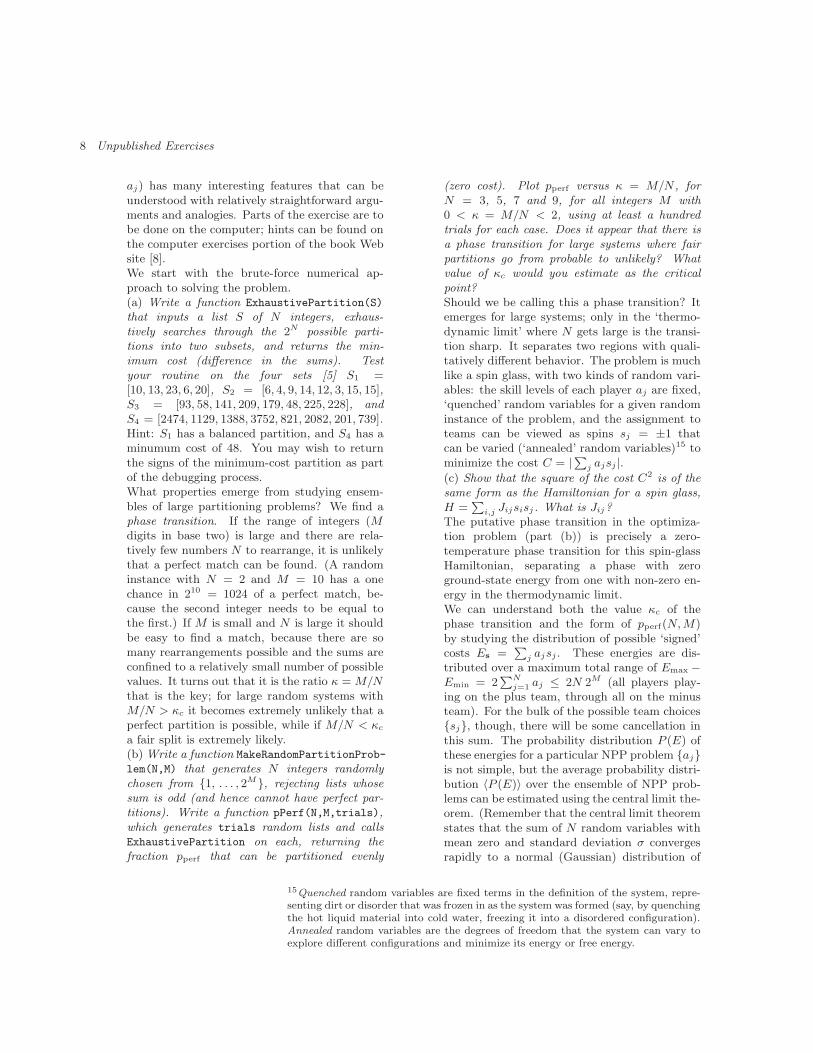
zero radius of convergence.18 (Condensedmatter) ©3In this exercise, we shall use methods from quan-tum field theory to tie together two topics whichAmerican science and engineering students studyin their first year of college: Hooke’s law and theconvergence of infinite series.Consider a large steel cube, stretched by a mod-erate strain ǫ = ∆L/L (Figure N.1). You mayassume ǫ ≪ 0.1%, where we can ignore plasticdeformation.(a) At non-zero temperature, what is the equilib-rium ground state for the cube as L → ∞ forfixed ǫ? (Hints: Remember, or show, that thefree energy per unit (undeformed) volume of thecube is 1/2Y ǫ2. Notice figure N.2 as an alternativecandidate for the ground state.) For steel, withY = 2 × 10¹¹ N/m2, γ ≈ 2.5 J/m2,19 and den-sity ρ = 8000 kg/m3, how much can we stretch abeam of length L = 10 m before the equilibriumlength is broken in two? How does this comparewith the amount the beam stretches under a loadequal to its own weight?
L/L = F/(YA)∆
MaterialElastic
Fig. N.1 Stretched block of elastic material,length L and width W , elongated vertically by a forceF per unit area A, with free side boundaries. Theblock will stretch a distance ∆L/L = F/Y A verti-cally and shrink by ∆W/W = σ ∆L/L in both hor-izontal directions, where Y is Young’s modulus andσ is Poisson’s ratio, linear elastic constants charac-teristic of the material. For an isotropic material,the other elastic constants can be written in termsof Y and σ; for example, the (linear) bulk modulusκlin = Y/3(1 − 2σ).
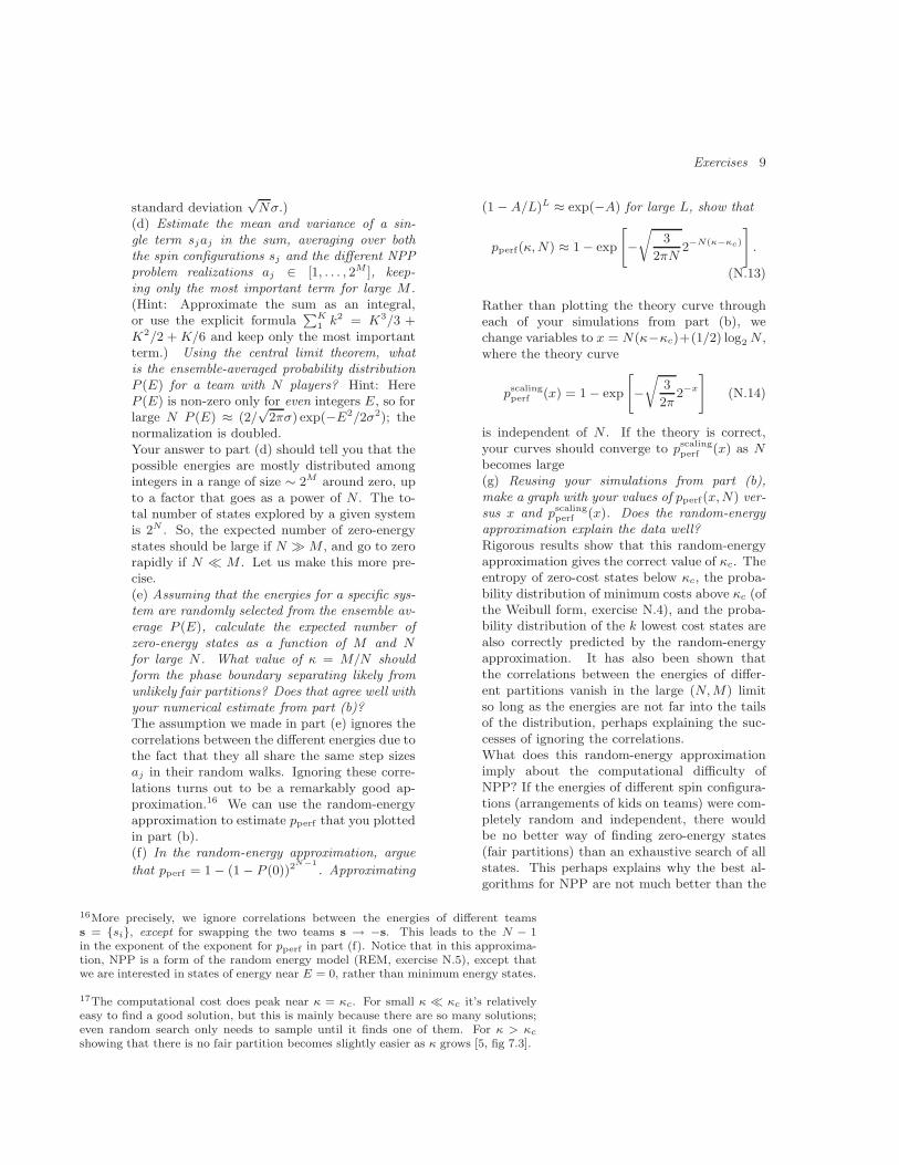
MaterialElastic
Aγ2Surface Energy
Fig. N.2 Fractured block of elastic material, as infigure N.1 but broken in two. The free energy hereis 2γA, where γ is the free energy per unit area A of(undeformed) fracture surface.
Why don’t bridges fall down? The beams in thebridge are in a metastable state. What is the bar-rier separating the stretched and fractured beamstates? Consider a crack in the beam, of lengthℓ. Your intuition may tell you that tiny crackswill be harmless, but a long crack will tend togrow at small external stress.For convenient calculations, we will now switchproblems from a stretched steel beam to a tauttwo-dimensional membrane under an isotropictension, a negative pressure P < 0. That is, weare calculating the rate at which a balloon willspontaneously pop due to thermal fluctuations.
18This exercise draws heavily on Alex Buchel’s work [1, 2].19This is the energy for a clean, flat [100] surface, a bit more than 1eV/surfaceatom [9]. The surface left by a real fracture in (ductile) steel will be rugged andseverely distorted, with a much higher energy per unit area. This is why steel ismuch harder to break than glass, which breaks in a brittle fashion with much lessenergy left in the fracture surfaces.
Exercises 11
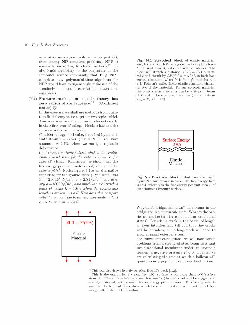
P < 0
Crack length
Fig. N.3 Critical crack of length ℓ, in a two-dimensional material under isotropic tension (neg-ative hydrostatic pressure P < 0).
The crack costs a surface free energy 2αℓ, whereα is the free energy per unit length of membraneperimeter. A detailed elastic theory calculationshows that a straight crack of length ℓ will re-lease a (Gibbs free) energy πP 2(1 − σ2)ℓ2/4Y .(b) What is the critical length ℓc of the crack,at which it will spontaneously grow rather thanheal? What is the barrier B(P ) to crack nucle-ation? Write the net free energy change in termsof ℓ, ℓc, and α. Graph the net free energy change∆G due to the the crack, versus its length ℓ.The point at which the crack is energetically fa-vored to grow is called the Griffiths threshold, ofconsiderable importance in the study of brittlefracture.The predicted fracture nucleation rate R(P ) perunit volume from homogeneous thermal nucle-ation of cracks is thus
R(P ) = (prefactors) exp(−B(P )/kBT ). (N.15)
One should note that thermal nucleation of frac-ture in an otherwise undamaged, undisorderedmaterial will rarely be the dominant failuremode. The surface tension is of order an eV perbond (> 103 K/A), so thermal cracks of arealarger than tens of bond lengths will have insur-mountable barriers even at the melting point.Corrosion, flaws, and fatigue will ordinarily leadto structural failures long before thermal nucle-ation will arise.
Advanced topic: Elastic theory has zero radius ofconvergence.
Many perturbative expansions in physics havezero radius of convergence. The most preciselycalculated quantity in physics is the gyromag-netic ratio of the electron [7]
(g − 2)theory = α/(2π) − 0.328478965 . . . (α/π)2
+ 1.181241456 . . . (α/π)3
− 1.4092(384)(α/π)4
+ 4.396(42) × 10−12 (N.16)
a power series in the fine structure constantα = e2/~c = 1/137.035999 . . . . (The last term isan α-independent correction due to other kindsof interactions.) Freeman Dyson gave a wonder-ful argument that this power-series expansion,and quantum electrodynamics as a whole, haszero radius of convergence. He noticed that thetheory is sick (unstable) for any negative α (cor-responding to a pure imaginary electron chargee). The series must have zero radius of conver-gence since any circle in the complex plane aboutα = 0 includes part of the sick region.How does Dyson’s argument connect to fracturenucleation? Fracture at P < 0 is the kind of in-stability that Dyson was worried about for quan-tum electrodynamics for α < 0. It has impli-cations for the convergence of nonlinear elastictheory.Hooke’s law tells us that a spring stretchesa distance proportional to the force applied:x − x0 = F/K, defining the spring constant1/K = dx/dF . Under larger forces, the Hooke’slaw will have corrections with higher powers ofF . We could define a ‘nonlinear spring constant’K(F ) by
1
K(F )=
x(F ) − x(0)
F= k0 + k1F + . . . (N.17)
Instead of a spring constant, we’ll calculate anonlinear version of the bulk modulus κnl(P )giving the pressure needed for a given fractionalchange in volume, ∆P = −κ∆V/V . The linearisothermal bulk modulus20 is given by 1/κlin =−(1/V )(∂V /∂P )|T ; we can define a nonlineargeneralization by
1
κnl(P )= − 1
V (0)
V (P ) − V (0)
P
= c0 + c1P + c2P2 + · · · + cNP N + · · ·
(N.18)
20Warning: For many purposes (e.g. sound waves) one must use the adiabatic elasticconstant 1/κ = −(1/V )(∂V /∂P )|S . For most solids and liquids these are nearly thesame.
12 Unpublished Exercises
This series can be viewed as higher and higher-order terms in a nonlinear elastic theory.(c) Given your argument in part (a) about thestability of materials under tension, would Dysonargue that the series in eqn N.18 has a zero or anon-zero radius of convergence?In Exercise 1.5 we saw the same argument holdsfor Stirling’s formula for N !, when extendedto a series in 1/N ; any circle in the com-plex 1/N plane contains points 1/(−N) fromlarge negative integers, where we can show that(−N)! = ∞. These series are asymptotic expan-sions. Convergent expansions
P
cnxn convergefor fixed x as n → ∞; asymptotic expansionsneed only converge to order O(xn+1) as x → 0for fixed n. Hooke’s law, Stirling’s formula, andquantum electrodynamics are examples of howimportant, powerful, and useful asymptotic ex-pansions can be.Buchel [1, 2], using a clever trick from field the-ory [12, Chapter 40], was able to calculate thelarge-order terms in elastic theory, essentially bydoing a Kramers–Kronig transformation on yourformula for the decay rate (eqn N.15) in part (b).His logic works as follows.• The Gibbs free energy density G of themetastable state is complex for negative P . Thereal and imaginary parts of the free energy forcomplex P form an analytic function (at leastin our calculation) except along the negative Paxis, where there is a branch cut.• Our isothermal bulk modulus for P > 0 canbe computed in terms of G = G/V (0). SincedG = −S dT +V dP +µ dN , V (P ) = (∂G/∂P )|Tand hence21
1
κnl(P )= − 1
V (0)
(∂G/∂P )|T − V (0)
P
= − 1
P
„
∂G∂P
˛
˛
˛
˛
T
− 1
«
. (N.19)
(d) Write the coefficients cn of eqn N.18 in termsof the coefficients gm in the nonlinear expansion
G(P ) =X
gmP m. (N.20)
• The decay rate R(P ) per unit volume is propor-tional to the imaginary part of the free energy
Im[G(P )], just as the decay rate Γ for a quan-tum state is related to the imaginary part i~Γ ofthe energy of the resonance. More specifically,for P < 0 the imaginary part of the free energyjumps as one crosses the real axis:
Im[G(P ± iǫ)] = ±(prefactors)R(P ). (N.21)
PCFRe[P]
Im[P]
A
EBD 0
Fig. N.4 Contour integral in complex pres-
sure. The free energy density G of the elastic mem-brane is analytic in the complex P plane except alongthe negative P axis. This allows one to evaluate G atpositive pressure P0 (where the membrane is stableand G is real) with a contour integral as shown.
• Buchel then used Cauchy’s formula to evaluatethe real part of G in terms of the imaginary part,and hence the decay rate R per unit volume:
G(P0) =1
2πi
I
ABCDEF
G(P )
P − P0dP
=1
2πi
Z 0
B
G(P + iǫ) − G(P − iǫ)
P − P0dP
+
Z
EF A
+
Z
BCD
=1
π
Z 0
B
Im[G(P + iǫ)]
P − P0dP
+ (unimportant) (N.22)
where the integral over the small semicircle van-ishes as its radius ǫ → 0 and the integral over thelarge circle is convergent and hence unimportantto high-order terms in perturbation theory.
21Notice that this is not the (more standard) pressure-dependent linear bulk modulus,κlin(P ) which is given by 1/κlin(P ) = −(1/V )(∂V /∂P )|T = −(1/V )(∂2G/∂P 2)|T .This would also have a Taylor series in P with zero radius of convergence at P = 0,but it has a different interpretation; κnl(P ) is the nonlinear response at P = 0, whileκlin(P ) is the pressure-dependent linear response.
Exercises 13
The decay rate (eqn N.15) for P < 0 should beof the form
R(P ) ∝ (prefactors) exp(−D/P 2), (N.23)
where D is some constant characteristic of thematerial. (You may use this to check your an-swer to part (b).)(e) Using eqns. N.21, N.22, and N.23, and as-suming the prefactors combine into a constantA, write the free energy for P0 > 0 as an inte-gral involving the decay rate over −∞ < P < 0.Expanding 1/(P −P0) in a Taylor series in pow-ers of P0, and assuming one may exchange sumsand integration, find and evaluate the integral forgm in terms of D and m. Calculate from gm thecoefficients cn, and then use the ratio test to cal-culate the radius of convergence of the expansionfor 1/κnl(P ), eqn N.18. (Hints: Use a table ofintegrals, a computer algebra package, or changevariable P = −
p
D/t to make your integral intothe Γ function,
Γ(z) = (z − 1)! =
Z ∞
0
tz−1 exp(−t)dt. (N.24)
If you wish, you may use the ratio test on everysecond term, so the radius of convergence is thevalue limn→∞
p
|cn/cn+2|.)(Why is this approximate calculation trustwor-thy? Your formula for the decay rate is valid onlyup to prefactors that may depend on the pres-sure; this dependence (some power of P ) won’tchange the asymptotic ratio of terms cn. Yourformula for the decay rate is an approximation,but one which becomes better and better forsmaller values of P ; the integral for the high-order terms gm (and hance cn) is concentratedat small P , so your approximation is asymptot-ically correct for the high order terms.)Thus the decay rate of the metastable state canbe used to calculate the high-order terms in per-turbation theory in the stable phase! This isa general phenomena in theories of metastablestates, both in statistical mechanics and in quan-tum physics.
(N.8) Extreme value statistics: Gumbel,
Weibull, and Frechet. (Mathematics, Statis-tics, Engineering) ©3Extreme value statistics is the study of the max-imum or minimum of a collection of randomnumbers. It has obvious applications in the in-surance business (where one wants to know thebiggest storm or flood in the next decades, see
Exercise N.3) and in the failure of large sys-tems (where the weakest component or flaw leadsto failure, see Exercise N.4). Recently extremevalue statistics has become of significant impor-tance in bioinformatics. (In guessing the func-tion of a new gene, one often searches entiregenomes for good matches (or alignments) to thegene, presuming that the two genes are evolu-tionary descendents of a common ancestor andhence will have similar functions. One mustunderstand extreme value statistics to evaluatewhether the best matches are likely to arise sim-ply at random.)The limiting distribution of the biggest or small-est of N random numbers as N → ∞ takes one ofthree universal forms, depending on the proba-bility distribution of the individual random num-bers. In this exercise we understand these formsas fixed points in a renormalization group.Given a probability distribution ρ1(x), we definethe cumulative distribution function (CDF) asF1(x) =
R x
−∞ρ(x′) dx′. Let us define ρN(x) to
be the probability density that, out of N randomvariables, the largest is equal to x. Let FN(x) tobe the corresponding CDF.(a) Write a formula for F2N (x) in terms ofFN (x). If FN (x) = exp(−gN(x)), show thatg2N (x) = 2gN (x).Our renormalization group coarse-graining oper-ation will remove half of the variables, throwingaway the smaller of every pair, and returningthe resulting new probability distribution. Interms of the function g(x) = − log
R x
−∞ρ(x′)dx′,
it therefore will return a rescaled version of the2g(x). This rescaling is necessary because, asthe sample size N increases, the maximum willdrift upward—only the form of the probabilitydistribution stays the same, the mean and widthcan change. Our renormalization-group coarse-graining operation thus maps function space intoitself, and is of the form
T [g](x) = 2g(ax + b). (N.25)
(This renormalization group is the same as thatwe use for sums of random variables in Exer-cise 12.11 where g(k) is the logarithm of theFourier transform of the probability density.)There are three distinct types of fixed-point dis-tributions for this renormalization group trans-formation, which (with an appropriate linearrescaling of the variable x) describe most ex-treme value statistics. The Gumbel distribution
14 Unpublished Exercises
(Exercise N.3) is of the form
Fgumbel(x) = exp(− exp(−x))
ρgumbel(x) = exp(−x) exp(− exp(−x)).
ggumbel(x) = exp(−x)
The Weibull distribution (Exercise N.4) is of theform
Fweibull(x) =
(
exp(−(−x)α) x < 0
1 x ≥ 0
gweibull(x) =
(
(−x)α x < 0
0 x ≥ 0,
(N.26)
and the Frechet distribution is of the form
Ffrechet(x) =
(
0 x ≤ 0
exp(−x−α) x > 0
gfrechet(x) =
(
∞ x < 0
x−α x ≥ 0,
(N.27)
where α > 0 in each case.(b) Show that these distributions are fixed pointsfor our renormalization-group transformationeqn N.25. What are a and b for each distribu-tion, in terms of α?In parts (c) and (d) you will show that there areonly these three fixed points g∗(x) for the renor-malization transformation, T [g∗](x) = 2g∗(ax +b), up to an overall linear rescaling of the vari-able x, with some caveats. . .(c) First, let us consider the case a 6= 1. Showthat the rescaling x → ax + b has a fixed pointx = µ. Show that the most general form for thefixed-point function is
g∗(µ ± z) = zα′
p±(γ log z) (N.28)
for z > 0, where p± is periodic and α′ and γ areconstants such that p± has period equal to one.(Hint: Assume p(y) ≡ 1, find α′, and then show
g∗/zα′
is periodic.) What are α′ and γ? Whichchoice for a, p+, and p− gives the Weibull dis-tribution? The Frechet distribution?Normally the periodic function p(γ log(x − µ))is assumed or found to be a constant (some-
times called 1/β, or 1/βα′
). If it is not constant,then the probability density must have an infi-nite number of oscillations as x → µ, forming aweird essential singularity.
(d) Now let us consider the case a = 1. Showagain that the fixed-point function is
g∗(x) = e−x/βp(x/γ) (N.29)
with p periodic of period one, and with suitableconstants β and γ. What are the constants interms of b? What choice for p and β yields theGumbel distribution?Again, the periodic function p is often assumeda constant (eµ), for reasons which are not as ob-vious as in part (c).What are the domains of attraction of the threefixed points? If we want to study the maximumof many samples, and the initial probability dis-tribution has F (x) as its CDF, to which universalform will the extreme value statistics converge?Mathematicians have sorted out these questions.If ρ(x) has a power-law tail, so 1− F (x) ∝ x−α,then the extreme value statistics will be of theFrechet type, with the same α. If the initialprobability distribution is bounded above at µand if 1−F (µ−y) ∝ yα, then the extreme valuestatistics will be of the Weibull type. (More com-monly, Weibull distributions arise as the small-est value from a distribution of positive randomnumbers, Exercise N.4.) If the probability distri-bution decays faster than any polynomial (say,exponentially) then the extreme value statisticswill be of the Gumbel form [10, section 8.2].(Gumbel extreme-value statistics can also arisefor bounded random variables if the probabilitydecays to zero faster than a power law at thebound [10]).
(N.9) Cardiac dynamics.22 (Computation, Biol-ogy, Complexity) ©4Reading: References [6, 11], Niels Otani,various web pages on cardiac dynamics,http://otani.vet.cornell.edu, and Arthur T.Winfree, ‘Varieties of spiral wave behav-ior: An experimentalist’s approach to thetheory of excitable media’, Chaos, 1, 303-334 (1991). See also spiral waves in Dic-tyostelium by Bodenschatz and Franck,http://newt.ccmr.cornell.edu/Dicty/diEp47A.movand http://newt.ccmr.cornell.edu/Dicty/diEp47A.avi.The cardiac muscle is an excitable medium.In each heartbeat, a wave of excitation passesthrough the heart, compressing first the atriawhich pushes blood into the ventricles, and then
22This exercise and the associated software were developed in collaboration withChristopher Myers.
Exercises 15
compressing the ventricles pushing blood intothe body. In this exercise we will study sim-plified models of heart tissue, that exhibit spiralwaves similar to those found in arrhythmias.An excitable medium is one which, when trig-gered from a resting state by a small stimulus, re-sponds with a large pulse. After the pulse thereis a refractory period during which it is difficultto excite a new pulse, followed by a return to theresting state. The FitzHugh-Nagumo equationsprovide a simplified model for the excitable hearttissue:23
∂V
∂t= ∇2V +
1
ǫ(V − V 3/3 − W )
∂W
∂t= ǫ(V − γW + β), (N.30)
where V is the transmembrane potential, W isthe recovery variable, and ǫ = 0.2, γ = 0.8, andβ = 0.7 are parameters. Let us first explore thebehavior of these equations ignoring the spatialdependence (dropping the ∇2V term, appropri-ate for a small piece of tissue). The dynamicscan be visualized in the (V, W ) plane.(a) Find and plot the nullclines of the FitzHugh-Nagumo equations: the curves along whichdV/dt and dW/dt are zero (ignoring ∇2V ). Theintersection of these two nullclines representsthe resting state (V ∗, W ∗) of the heart tissue.We apply a stimulus to our model by shiftingthe transmembrane potential to a larger value—running from initial conditions (V ∗ + ∆, W ∗).Simulate the equations for stimuli ∆ of varioussizes; plot V and W as a function of time t, andalso plot V (t) versus W (t) along with the null-clines. How big a stimulus do you need in orderto get a pulse?Excitable systems are often close to regimeswhere they develop spontaneous oscillations.Indeed, the FitzHugh-Nagumo equations areequivalent to the van der Pol equation (whicharose in the study of vacuum tubes), a standardsystem for studying periodic motion.(b) Try changing to β = 0.4. Does the system os-cillate? The threshold where the resting statebecomes unstable is given when the nullcline in-tersection lies at the minimum of the V nullcline,at βc = 7/15.Each portion of the tissue during a contractionwave down the heart is stimulated by its neigh-
bors to one side, and its pulse stimulates theneighbor to the other side. This triggering in ourmodel is induced by the Laplacian term ∇2V .We simulate the heart on a two-dimensional gridV (xi, yj , t), W (xi, yj , t), and calculate an ap-proximate Laplacian by taking differences be-tween the local value of V and values at neigh-boring points.There are two natural choices for this Laplacian.The five-point discrete Laplacian is generaliza-tion of the one-dimensional second derivative,∂2V /∂x2 ≈ (V (x+dx)−2V (x)+V (x−dx))/dx2:
∇2[5]V (xi, yi) ≈ (V (xi, yi+1) + V (xi, yi−1)
+ V (xi+1, yi) + V (xi−1, yi)
− 4V (xi, yi))/dx2
↔ 1
dx2
0
@
0 1 01 −4 10 1 0
1
A
(N.31)
where dx = xi+1 − xi = yi+1 − yi is the spac-ing between grid points and the last expressionis the stencil by which you multiply the pointand its neighbors by to calculate the Laplacian.The nine-point discrete Laplacian has been fine-tuned for improved circularly symmetry, withstencil
∇2[9]V (xi, yi) ↔
1
dx2
0
@
1/6 2/3 1/62/3 −10/3 2/31/6 2/3 1/6
1
A .
(N.32)We will simulate our partial-differential equation(PDE) on a square 100 × 100 grid with a gridspacing dx = 1.24 As is often done in PDEs,we will use the crude Euler time-step schemeV (t + ∆) ≈ V (t) + ∆∂V /∂t (see Exercise 3.12):we find ∆ ≈ 0.1 is the largest time step we canget away with. We will use ‘no-flow’ boundaryconditions, which we implement by setting theLaplacian terms on the boundary to zero (theboundaries, uncoupled from the rest of the sys-tem, will quickly turn to their resting state). Ifyou are not supplied with example code thatdoes the two-dimensional plots, you may findthem at the text web site [8].(c) Solve eqn N.30 for an initial condition equalto the fixed-point (V ∗, W ∗) except for a 10 × 10square at the origin, in which you should apply
23Nerve tissue is also an excitable medium, modeled using different Hodgkin-Huxley
equations.24Smaller grids would lead to less grainy waves, but slow down the simulation a lot.
16 Unpublished Exercises
a stimulus ∆ = 3.0. (Hint: Your simulationshould show a pulse moving outward from theorigin, disappearing as it hits the walls.)If you like, you can mimic the effects of thesinoatrial (SA) node (your heart’s natural pace-maker) by stimulating your heart model period-ically (say, with the same 10× 10 square). Real-istically, your period should be long enough thatthe old beat finishes before the new one starts.We can use this simulation to illustrate generalproperties of solving PDEs.(d) Accuracy. Compare the five and nine-pointLaplacians. Does the latter give better circu-lar symmetry? Stability. After running for awhile, double the time step ∆. How does the sys-tem go unstable? Repeat this process, reducing∆ until just before it goes nuts. Do you see in-accuracies in the simulation that foreshadow theinstability?This checkerboard instability is typical of PDEswith too high a time step. The maximum timestep in this system will go as dx2, the latticespacing squared—thus to make dx smaller by afactor of two and simulate the same area, youneed four times as many grid points and fourtimes as many time points—giving us a good rea-son for making dx as large as possible (correctingfor grid artifacts by using improved Laplacians).Similar but much more sophisticated tricks havebeen used recently to spectacularly increase theperformance of lattice simulations of the inter-actions between quarks [3].As mentioned above, heart arrhythmias are dueto spiral waves. To generate spiral waves we needto be able to start up more asymmetric states—stimulating several rectangles at different times.Also, when we generate the spirals, we wouldlike to emulate electroshock therapy by apply-ing a stimulus to a large region of the heart.We can do both by writing code to interactivelystimulate a whole rectangle at one time. Again,the code you have obtained from us should havehints for how to do this.(e) Add the code for interactively stimulating ageneral rectangle with an increment to V of size∆ = 3. Play with generating rectangles in differ-ent places while other pulses are going by: makesome spiral waves. Clear the spirals by giving astimulus that spans the system.There are several possible extensions of this
model, several of which involve giving our modelspatial structure that mimics the structure of theheart. (One can introduce regions of inactive‘dead’ tissue. One can introduce the atrium andventricle compartments to the heart, with theSA node in the atrium and an AV node connect-ing the two chambers . . . ) Niels Otani has anexercise with further explorations of a numberof these extensions, which we link to from theCardiac Dynamics web site.
(N.10) Quantum dissipation from phonons.
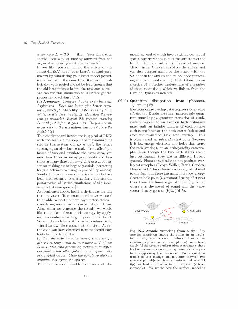
(Quantum) ©2Electrons cause overlap catastrophes (X-ray edgeeffects, the Kondo problem, macroscopic quan-tum tunneling); a quantum transition of a sub-system coupled to an electron bath ordinarilymust emit an infinite number of electron-holeexcitations because the bath states before andafter the transition have zero overlap. Thisis often called an infrared catastrophe (becauseit is low-energy electrons and holes that causethe zero overlap), or an orthogonality catastro-phe (even though the two bath states aren’tjust orthogonal, they are in different Hilbertspaces). Phonons typically do not produce over-lap catastrophes (Debye–Waller, Frank–Condon,Mossbauer). This difference is usually attributedto the fact that there are many more low-energyelectron-hole pairs (a constant density of states)than there are low-energy phonons (ωk ∼ ck,where c is the speed of sound and the wave-vector density goes as (V/2π)3d3k).
Vo
Qo
AFM /STM tip AFM /STM tip
Substrate Substrate
Fig. N.5 Atomic tunneling from a tip. Anyinternal transition among the atoms in an insula-tor can only exert a force impulse (if it emits mo-mentum, say into an emitted photon), or a forcedipole (if the atomic configuration rearranges); theselead to non-zero phonon overlap integrals only par-tially suppressing the transition. But a quantumtransition that changes the net force between twomacroscopic objects (here a surface and a STMtip) can lead to a change in the net force (a forcemonopole). We ignore here the surface, modeling
25∗
Exercises 17
the force as exerted directly into the center of aninsulating elastic medium.25See “Atomic Tunnelingfrom a STM/AFM Tip: Dissipative Quantum Effectsfrom Phonons” Ard A. Louis and James P. Sethna,Phys. Rev. Lett. 74, 1363 (1995), and “Dissipativetunneling and orthogonality catastrophe in molecu-lar transistors”, S. Braig and K. Flensberg, Phys.
Rev. B 70, 085317 (2004).
However, the coupling strength to the low energyphonons has to be considered as well. Considera small system undergoing a quantum transitionwhich exerts a net force at x = 0 onto an insu-lating crystal:
H =X
k
p2k/2m + 1/2 mω2
kq2k + F · u0. (N.33)
Let us imagine a kind of scalar elasticity, toavoid dealing with the three phonon branches(two transverse and one longitudinal); we thusnaively write the displacement of the atom at lat-tice site xn as un = (1/
√N)
P
k qk exp(−ikxn)(with N the number of atoms), so qk =(1/
√N)
P
n un exp(ikxn).Substituting for u0 in the Hamiltonian and com-pleting the square, find the displacement ∆k ofeach harmonic oscillator. Write the formulafor the likelihood 〈F |0〉 that the phonons will allend in their ground states, as a product overk of the phonon overlap integral exp(−∆2
k/8a2k)
(with ak =p
~/2mωk the zero-point motion inthat mode). Converting the product to the ex-ponential of a sum, and the sum to an integralP
k ∼ (V/(2π)3R
dk, do we observe an overlapcatastrophe?
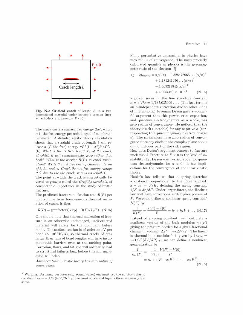
(N.11) The Gutenberg Richter law. (Scaling) ©3
4 5 6 7 8Magnitude
1
10
100
1000
10000
Num
ber
of e
arth
quak
es
0.0001 0.01 0.1 1.0 10.0Energy radiated (10
15 joules)
S -2/3
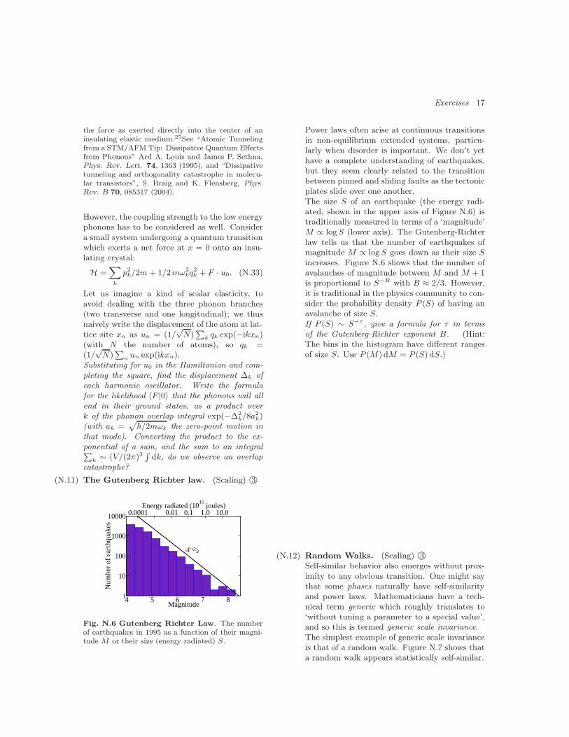
Fig. N.6 Gutenberg Richter Law. The numberof earthquakes in 1995 as a function of their magni-tude M or their size (energy radiated) S.
Power laws often arise at continuous transitionsin non-equilibrium extended systems, particu-larly when disorder is important. We don’t yethave a complete understanding of earthquakes,but they seem clearly related to the transitionbetween pinned and sliding faults as the tectonicplates slide over one another.The size S of an earthquake (the energy radi-ated, shown in the upper axis of Figure N.6) istraditionally measured in terms of a ‘magnitude’M ∝ log S (lower axis). The Gutenberg-Richterlaw tells us that the number of earthquakes ofmagnitude M ∝ log S goes down as their size Sincreases. Figure N.6 shows that the number ofavalanches of magnitude between M and M + 1is proportional to S−B with B ≈ 2/3. However,it is traditional in the physics community to con-sider the probability density P (S) of having anavalanche of size S.If P (S) ∼ S−τ , give a formula for τ in termsof the Gutenberg-Richter exponent B. (Hint:The bins in the histogram have different rangesof size S. Use P (M) dM = P (S) dS.)
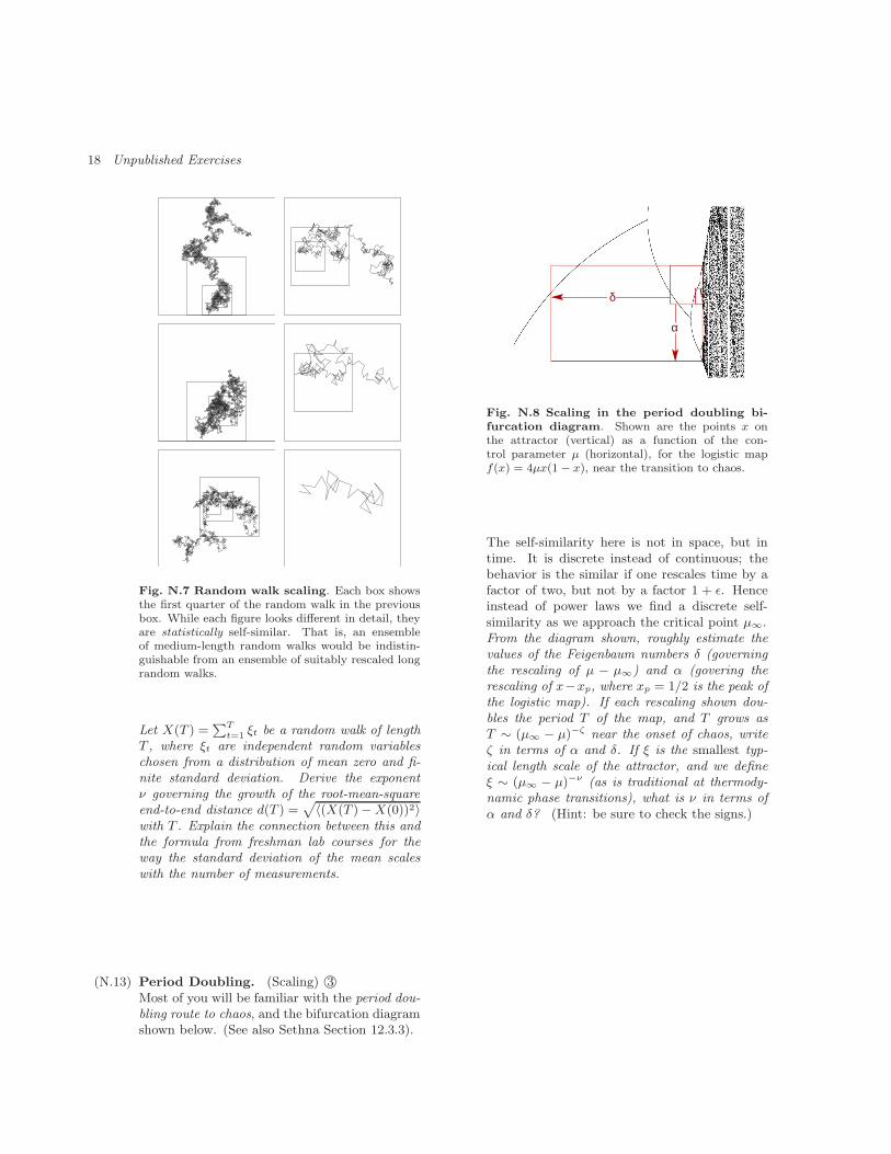
(N.12) Random Walks. (Scaling) ©3Self-similar behavior also emerges without prox-imity to any obvious transition. One might saythat some phases naturally have self-similarityand power laws. Mathematicians have a tech-nical term generic which roughly translates to‘without tuning a parameter to a special value’,and so this is termed generic scale invariance.The simplest example of generic scale invarianceis that of a random walk. Figure N.7 shows thata random walk appears statistically self-similar.
18 Unpublished Exercises
Fig. N.7 Random walk scaling. Each box showsthe first quarter of the random walk in the previousbox. While each figure looks different in detail, theyare statistically self-similar. That is, an ensembleof medium-length random walks would be indistin-guishable from an ensemble of suitably rescaled longrandom walks.
Let X(T ) =PT
t=1 ξt be a random walk of lengthT , where ξt are independent random variableschosen from a distribution of mean zero and fi-nite standard deviation. Derive the exponentν governing the growth of the root-mean-squareend-to-end distance d(T ) =
p
〈(X(T ) − X(0))2〉with T . Explain the connection between this andthe formula from freshman lab courses for theway the standard deviation of the mean scaleswith the number of measurements.
(N.13) Period Doubling. (Scaling) ©3Most of you will be familiar with the period dou-bling route to chaos, and the bifurcation diagramshown below. (See also Sethna Section 12.3.3).
δ
α
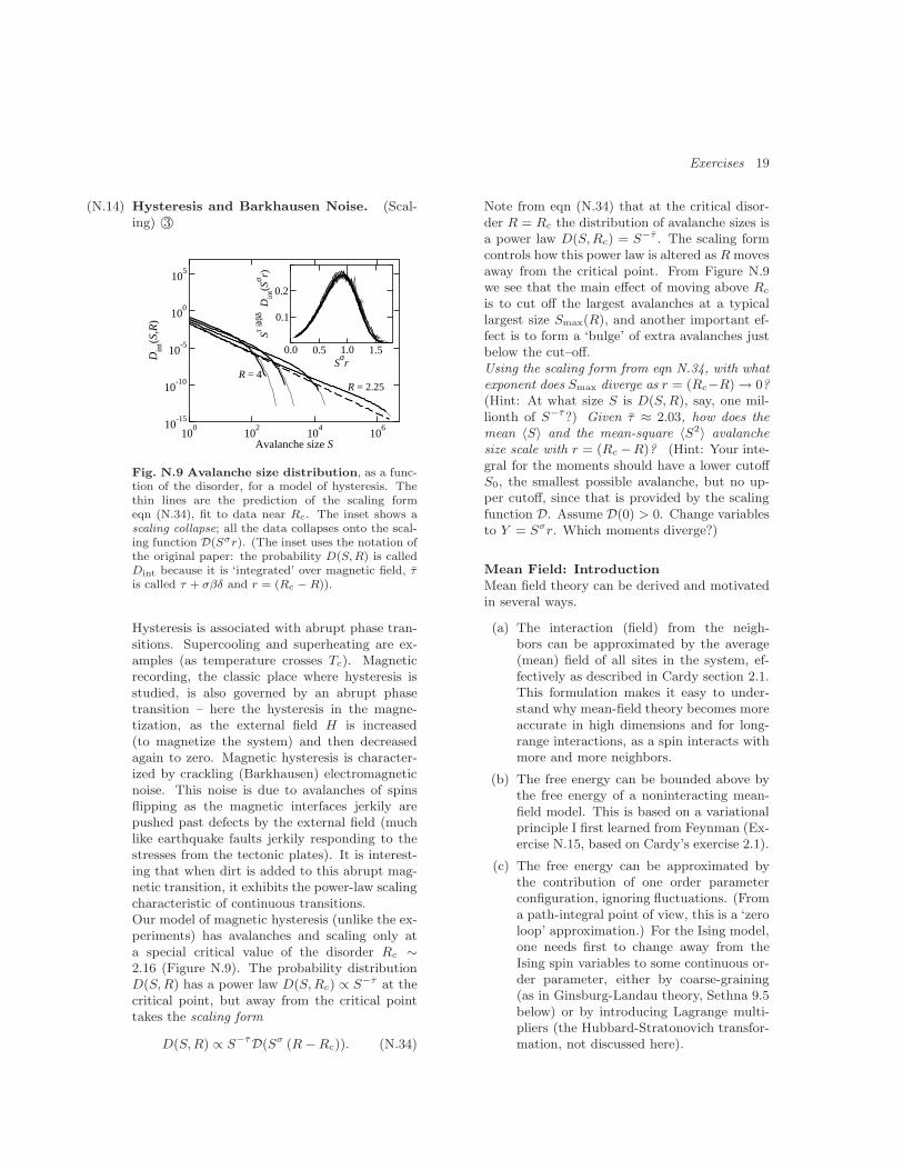
Fig. N.8 Scaling in the period doubling bi-
furcation diagram. Shown are the points x onthe attractor (vertical) as a function of the con-trol parameter µ (horizontal), for the logistic mapf(x) = 4µx(1 − x), near the transition to chaos.
The self-similarity here is not in space, but intime. It is discrete instead of continuous; thebehavior is the similar if one rescales time by afactor of two, but not by a factor 1 + ǫ. Henceinstead of power laws we find a discrete self-similarity as we approach the critical point µ∞.From the diagram shown, roughly estimate thevalues of the Feigenbaum numbers δ (governingthe rescaling of µ − µ∞) and α (govering therescaling of x−xp, where xp = 1/2 is the peak ofthe logistic map). If each rescaling shown dou-bles the period T of the map, and T grows asT ∼ (µ∞ − µ)−ζ near the onset of chaos, writeζ in terms of α and δ. If ξ is the smallest typ-ical length scale of the attractor, and we defineξ ∼ (µ∞ − µ)−ν (as is traditional at thermody-namic phase transitions), what is ν in terms ofα and δ? (Hint: be sure to check the signs.)
Exercises 19
(N.14) Hysteresis and Barkhausen Noise. (Scal-ing) ©3
100
102
104
106
Avalanche size S
10-15
10-10
10-5
100
105
Din
t(S,R
)
0.0 0.5 1.0 1.5S
σr
0.1
0.2
Sτ +
σβδ D
int(S
σ r)
R = 4R = 2.25
Fig. N.9 Avalanche size distribution, as a func-tion of the disorder, for a model of hysteresis. Thethin lines are the prediction of the scaling formeqn (N.34), fit to data near Rc. The inset shows ascaling collapse; all the data collapses onto the scal-ing function D(Sσr). (The inset uses the notation ofthe original paper: the probability D(S, R) is calledDint because it is ‘integrated’ over magnetic field, τis called τ + σβδ and r = (Rc − R)).
Hysteresis is associated with abrupt phase tran-sitions. Supercooling and superheating are ex-amples (as temperature crosses Tc). Magneticrecording, the classic place where hysteresis isstudied, is also governed by an abrupt phasetransition – here the hysteresis in the magne-tization, as the external field H is increased(to magnetize the system) and then decreasedagain to zero. Magnetic hysteresis is character-ized by crackling (Barkhausen) electromagneticnoise. This noise is due to avalanches of spinsflipping as the magnetic interfaces jerkily arepushed past defects by the external field (muchlike earthquake faults jerkily responding to thestresses from the tectonic plates). It is interest-ing that when dirt is added to this abrupt mag-netic transition, it exhibits the power-law scalingcharacteristic of continuous transitions.Our model of magnetic hysteresis (unlike the ex-periments) has avalanches and scaling only ata special critical value of the disorder Rc ∼2.16 (Figure N.9). The probability distributionD(S, R) has a power law D(S, Rc) ∝ S−τ at thecritical point, but away from the critical pointtakes the scaling form
D(S, R) ∝ S−τD(Sσ (R − Rc)). (N.34)
Note from eqn (N.34) that at the critical disor-der R = Rc the distribution of avalanche sizes isa power law D(S, Rc) = S−τ . The scaling formcontrols how this power law is altered as R movesaway from the critical point. From Figure N.9we see that the main effect of moving above Rc
is to cut off the largest avalanches at a typicallargest size Smax(R), and another important ef-fect is to form a ‘bulge’ of extra avalanches justbelow the cut–off.Using the scaling form from eqn N.34, with whatexponent does Smax diverge as r = (Rc−R) → 0?(Hint: At what size S is D(S, R), say, one mil-lionth of S−τ?) Given τ ≈ 2.03, how does themean 〈S〉 and the mean-square 〈S2〉 avalanchesize scale with r = (Rc −R)? (Hint: Your inte-gral for the moments should have a lower cutoffS0, the smallest possible avalanche, but no up-per cutoff, since that is provided by the scalingfunction D. Assume D(0) > 0. Change variablesto Y = Sσr. Which moments diverge?)
Mean Field: Introduction
Mean field theory can be derived and motivatedin several ways.
(a) The interaction (field) from the neigh-bors can be approximated by the average(mean) field of all sites in the system, ef-fectively as described in Cardy section 2.1.This formulation makes it easy to under-stand why mean-field theory becomes moreaccurate in high dimensions and for long-range interactions, as a spin interacts withmore and more neighbors.
(b) The free energy can be bounded above bythe free energy of a noninteracting mean-field model. This is based on a variationalprinciple I first learned from Feynman (Ex-ercise N.15, based on Cardy’s exercise 2.1).
(c) The free energy can be approximated bythe contribution of one order parameterconfiguration, ignoring fluctuations. (Froma path-integral point of view, this is a ‘zeroloop’ approximation.) For the Ising model,one needs first to change away from theIsing spin variables to some continuous or-der parameter, either by coarse-graining(as in Ginsburg-Landau theory, Sethna 9.5below) or by introducing Lagrange multi-pliers (the Hubbard-Stratonovich transfor-mation, not discussed here).
20 Unpublished Exercises
(d) The Hamiltonian can be approximated byan infinite-range model, where each spindoes interact with the average of all otherspins. Instead of an approximate calcu-lation for the exact Hamiltonian, this isan exact calculation for an approximateHamiltonian – and hence is guaranteedto be at least a sensible physical model.See Exercise N.16 for an application toavalanche statistics.
(e) The lattice of sites in the Hamiltonian canbe approximated as a branching tree (re-moving the loops) called the Bethe lattice(not described here). This yields a dif-ferent, solvable, mean-field theory, whichordinarily has the same mean-field criticalexponents but different non-universal fea-tures.
(N.15) Variational mean-field derivation. (Meanfield) ©3Just as the entropy is maximized by a uni-form probability distribution on the energy shellfor a fixed-energy (microcanonical) ensemble, itis a known fact that the Boltzmann distribu-tion exp(−βH)/Z minimizes the free energy Ffor a fixed-temperature (canonical) ensemble de-scribed by Hamiltonian energy function H. If ageneral ensemble ρ′ gives the probability of everystate X in a system, and we define for an observ-able B the average 〈B〉ρ′ =
P
X B(X)ρ′(X) thenwhat this says is that
F = − (1/β) logX
X
exp(−βH(X))
≤〈F 〉ρ′ = 〈E − TS〉ρ′
= 〈H〉ρ′ − T 〈S〉ρ′ (N.35)
Feynman, in his work on the polaron problem,derived a variational formula for what appearsto be a related problem. If we define 〈B〉H′ tobe the Boltzmann average of B under the hamil-tonian H′, Feynman says that
Tr e−βH ≥ Tr e−β(H′+〈H−H′〉H′ ). (N.36)
Feynman’s formula varies not among generalprobability distributions ρ′, but only among ap-proximating Hamiltonians H′.(a) Show that eqn N.35 implies eqn N.36. (Hint:〈S〉H′ is not dependent on H, and F ′ = E′ −T S′.)
(b: Cardy exercise 2.1) Derive the mean fieldequations for the Ising ferromagnet using Feyn-man’s inequality (eqn N.36), where H is the fullHamiltonian and H′ = h
P
i Si is a trial Hamil-tonian, with h chosen to maximize the right-handside.Notice that having a variational bound on thefree energy is not as useful as it sounds. Thefree energy itself is usually not of great inter-est; the objects of physical importance are al-most always derivatives (first derivatives like thepressure, energy and entropy, and second deriva-tives like the specific heat) or differences (tellingwhich phase is more stable). Knowing an upperbound to the free energy doesn’t tell us muchabout these other quantities. Like most varia-tional methods, mean-field theory is useful notbecause of its variational bound, but because (ifdone well) it provides qualitative insight into thebehavior.
(N.16) Avalanche Size Distribution. (Scaling func-tion) ©3One can develop a mean-field theory foravalanches in non-equilibrium disordered sys-tems by considering a system of N Ising spinscoupled to one another by an infinite-range in-teraction of strength J/N , with an external fieldH and each spin also having a local random fieldh:
H = −J0/NX
i,j
SiSj −X
i
(H + hi)Si. (N.37)
We assume that each spin flips over when it ispushed over; i.e., when its change in energy
H loci =
∂H∂Si
= J0/NX
j
Sj + H + hi
= J0m + H + hi
changes sign.26 Here m = (1/N)P
j Sj is theaverage magnetization of the system. All spinsstart by pointing down. A new avalanche islaunched when the least stable spin (the un-flipped spin of largest local field) is flippedby increasing the external field H . Each spinflip changes the magnetization by 2/N . If themagnetization change from the first spin flip isenough to trigger the next-least-stable spin, theavalanche will continue.
26We ignore the self-interaction, which is unimportant at large N
Exercises 21
We assume that the probability density for therandom field ρ(h) during our avalanche is a con-stant
ρ(h) = (1 + t)/(2J0). (N.38)
The constant t will measure how close the den-sity is to the critical density 1/(2J0).(a) Show that at t = 0 each spin flip will trig-ger on average one other spin to flip, for largeN . Can you qualitatively explain the differencebetween the two phases with t < 0 and t > 0?We can solve exactly for the probability D(S, t)of having an avalanche of size S. To have anavalanche of size S triggered by a spin with ran-dom field h, you must have precisely S − 1 spinswith random fields in the range h, h+2J0S/N(triggered when the magnetization changes by2S/N). The probability of this is given by thePoisson distribution. In addition, the randomfields must be arranged so that the first spin trig-gers the rest. The probability of this turns outto be 1/S.(b) By imagining putting periodic boundary con-ditions on the interval h, h + 2J0S/N, arguethat exactly one spin out of the group of S spinswill trigger the rest as a single avalanche. (Hintfrom Ben Machta: For simplicity, we may as-sume27 the avalanche starts at H = m = 0. Tryplotting the local field H loc(h′) = J0m(h′) + h′
that a spin with random field h′ would feel ifthe spins between h′ and h were flipped. Howwould this function change if we shuffle all therandom fields around the periodic boundary con-ditions?)(c) Show that the distribution of avalanche sizesis thus
D(S, t) =SS−1
S!(t + 1)S−1e−S(t+1). (N.39)
With t small (near to the critical density) and forlarge avalanche sizes S we expect this to have ascaling form:
D(S, t) = S−τD(S/t−x) (N.40)
for some mean-field exponent x. That is, tak-ing t → 0 and S → ∞ along a path with Stx
fixed, we can expand D(S, t) to find the scalingfunction.
(d) What is the scaling function D? What are τand x?This is a bit tricky to get right. Let’s check it bydoing the plots.(e) Plot SτD(S, t) versus Y = S/t−x for t = 0.2,0.1, and 0.05 in the range Y ∈ (0, 10). Does itconverge to D(Y )?(See “Hysteresis and hierarchies, dynamics ofdisorder-driven first-order phase transforma-tions”, J. P. Sethna, K. Dahmen, S. Kartha,J. A. Krumhansl, B. W. Roberts, and J. D.Shore, PRL 70, 3347 (1993) for more informa-tion.)
(N.17) Ising Lower Critical Dimension. (Dimen-sion dependence) ©3What is the lower critical dimension of the Isingmodel? If the total energy ∆E needed to destroylong-range order is finite as the system size Lgoes to infinity, and the associated entropy growswith system size, then surely long-range order ispossible only at zero temperature.(a) Ising model in D dimensions. Considerthe Ising model in dimension D on a hypercubiclattice of length L on each side. Estimate theenergy28 needed to create a domain wall splittingthe system into two equal regions (one spin up,the other spin down). In what dimension willthis wall have finite energy as L → ∞? Suggesta bound for the lower critical dimension of theIsing model.The scaling at the lower critical dimension is of-ten unusual, with quantities diverging in waysdifferent from power laws as the critical temper-ature Tc is approached.(b) Correlation length in 1D Ising model.
Estimate the number of domain walls at tempera-ture T in the 1D Ising model. How does the cor-relation length ξ (the distance between domainwalls) grow as T → Tc = 0? (Hint: Changevariables to ηi = SiSi+1, which is −1 if there isa domain wall between sites i and i+1.) The cor-relation exponent ν satisfying ξ ∼ (T − Tc)
−ν is1, ∼ 0.63, and 1/2 in dimensions D = 2, 3, and≥ 4, respectively. Is there an exponent ν govern-ing this divergence in one dimension? How doesν behave as D → 1?
27Equivalently, measure the random fields with respect to h0 of the triggering spin,and let m be the magnetization change since the avalanche started.28Energy, not free energy! Think about T = 0.
22 Unpublished Exercises
(N.18) XY Lower Critical Dimension and the
Mermin-Wagner Theorem. (Dimension de-pendence) ©3Consider a model of continuous unit-length spins(e.g., XY or Heisenberg) on a D-dimensional hy-percubic lattice of length L. Assume a nearest-neighbor ferromagnetic bond energy
− J Si · Sj . (N.41)
Estimate the energy needed to twist the spinsat one boundary 180 with respect to the otherboundary (the energy difference between periodicand antiperiodic boundary conditions along oneaxis). In what dimension does this energy stayfinite in the thermodynamic limit L → ∞? Sug-gest a bound for the lower critical dimension forthe emergence of continuous broken symmetriesin models of this type.Note that your argument produces only onethick domain wall (unlike the Ising model, wherethe domain wall can be placed in a variety ofplaces). If in the lower critical dimension its en-ergy is fixed as L → ∞ at a value large com-pared to kBT , one could imagine most of thetime the order might maintain itself across thesystem. The actual behavior of the XY model inits lower critical dimension is subtle.On the one hand, there cannot be long-rangeorder. This can be seen convincingly, but notrigorously, by estimating the effects of fluctu-ations at finite temperature on the order pa-rameter, within linear response. Pierre Hohen-berg, David Mermin and Herbert Wagner provedit rigorously (including nonlinear effects) usingan inequality due to Bogoliubov. One shouldnote, though, that the way this theorem is usu-ally quoted (”continuous symmetries cannot bespontaneously broken at finite temperatures inone and two dimensions”) is too general. Inparticular, for two-dimensional crystals one haslong-range order in the crystalline orientations,although one does not have long-range brokentranslational order.On the other hand, the XY model does have aphase transition in its lower critical dimensionat a temperature Tc > 0. The high-temperaturephase is a traditional paramagentic phase, withexponentially decaying correlations between ori-entations as the distance increases. The low-temperature phase indeed lacks long-range or-der, but it does have a stiffness – twisting thesystem (as in your calculation above) by 180
costs a free energy that goes to a constant asL → ∞. In this stiff phase the spin-spin correla-tions die away not exponentially, but as a powerlaw.The corresponding Kosterlitz–Thouless phasetransition has subtle, fascinating scaling prop-erties. Interestingly, the defect that destroys thestiffness (a vortex) in the Kosterlitz–Thoulesstransition does not have finite energy as the sys-tem size L gets large. We shall see that its energygrows ∼ log L, while its entropy grows ∼ T log L,so entropy wins over energy as the temperaturerises, even though the latter is infinite.
(N.19) Long-range Ising. (Dimension depen-dence) ©3The one-dimensional Ising model can have afinite-temperature transition if we give each spinan interaction with distant spins.Long-range forces in the 1d Ising model.
Consider an Ising model in one dimension, withlong-range ferromagnetic bonds
H =X
i>j
J
|i − j|σ SiSj . (N.42)
For what values of σ will a domain wall betweenup and down spins have finite energy? Suggest abound for the ‘lower critical power law’ for thislong-range one-dimensional Ising model, belowwhich a ferromagnetic state is only possible whenthe temperature is zero. (Hint: Approximatethe sum by a double integral. Avoid i = j.)The long-range 1D Ising model at the lower crit-ical power law has a transition that is closely re-lated to the Kosterlitz-Thouless transition. It isin the same universality class as the famous (butobscure) Kondo problem in quantum phase tran-sitions. And it is less complicated to think aboutand less complicated to calculate with than ei-ther of these other two cases.
(N.20) Equilibrium Crystal Shapes. (Crystalshapes) ©3What is the equilibrium shape of a crys-tal? There are nice experiments on singlecrystals of salt, gold, and lead crystals (seehttp://www.lassp.cornell.edu/sethna/CrystalShapes/Equilibrium Crystal Shapes.html).They show beautiful faceted shapes, formed bycarefully annealing single crystals to equilibriumat various temperatures. The physics governingthe shape involves the anisotropic surface ten-sion γ(n) of the surface, which depends on the
Exercises 23
orientation n of the local surface with respect tothe crystalline axes.We can see how this works by considering theproblem for atoms on a 2D square lattice withnear-neighbor interations (a lattice gas which wemap in the standard way onto a conserved-orderparameter Ising model). Here γ(θ) becomes theline tension between the up and down phases– the interfacial free energy per unit length be-tween an up-spin and a down-spin phase. Wedraw heavily on Craig Rottman and MichaelWortis, Phys. Rev. B 24, 6274 (1981), and onW. K. Burton, N. Cabrera and F. C. Frank, Phil.Trans. R. Soc. Lond. A 243 299-358 (1951).(a) Interfacial free energy, T = 0. Consider aninterface at angle θ between up spins and downspins. Show that the energy cost per unit lengthof the interface is
γ0(θ) = 2J(cos(|θ|) + sin(|θ|)), (N.43)
where length is measured in lattice spacings.(b) Interfacial free energy, low T . Consider aninterface at angle θ = arctan N/M , connect-ing the origin to the point (M, N). At zerotemperature, this will be an ensemble of stair-cases, with N steps upward and M steps forward.Show that the total number of such staircases is(M + N)!/(M !N !). Hint: The number of waysof putting k balls into ℓ jars allowing more thanone ball per jar (the ‘number of combinationswith repetition’) is (k + ℓ− 1)!/(k!(ℓ− 1)!. Lookup the argument. Using Stirling’s formula, showthat the entropy per unit length is
s0(θ) =kB
“
(cos(|θ|) + sin(|θ|))log (cos(|θ|) + sin(|θ|))
− cos(|θ|) log(cos(|θ|)) (N.44)
− sin(|θ|) log(sin(|θ|))”
.
How would we generate an equilibrium crystalfor the 2D Ising model? (For example, see “TheGibbs-Thomson formula at small island sizes
- corrections for high vapour densities” Badri-narayan Krishnamachari, James McLean, Bar-bara Cooper, and James P. Sethna, Phys. Rev.B 54, 8899 (1996).) Clearly we want a conservedorder parameter simulation (otherwise the up-spin ‘crystal’ cluster in a down-spin ‘vapor’ envi-ronment would just flip over). The tricky part isthat an up-spin cluster in an infinite sea of down-spins will evaporate – it’s unstable.29 The key isto do a simulation below Tc, but with a net (con-served) negative magnetization slightly closer tozero that expected in equilibrium. The extraup-spins will (in equilibrium) mostly find one an-other, forming a cluster whose time-average willgive an equilibrium crystal.Rottman and Wortis tell us that the equilibriumcrystal shape (minimizing the perimeter energyfor fixed crystal area) can be found as a para-metric curve
x = cos(θ)γ(θ, T ) − sin(θ)dγ
dθ
y = sin(θ)γ(θ, T ) + cos(θ)dγ
dθ
where γ(θ, T ) = γ0(θ) − Ts(θ, T ) is the free en-ergy per unit length of the interface. Derivingthis is cool, but somewhat complicated.30
(c) Wolff construction. Using the energy ofeqn N.43 and approximating the entropy atlow temperatures with the zero-temperature formeqn N.44, plot the Wulff shape for T = 0.01, 0.1,0.2, 0.4, and 0.8J for one quadrant (0 < θ <π/2). Hint: Ignore the parts of the face outsidethe quadrant; they are artifacts of the low tem-perature approximation. Does the shape becomecircular31 near Tc = 2J/ log(1 +
√2) ∼ 2.269J?
Why not? If you’re ambitious, Rottman andWortis’s article above gives the exact interfacialfree energy for the 2D Ising model, which shouldfix this problem. What is the shape at low tem-peratures, where our approximation is good? Dowe ever get true facets? The approximationof the interface as a staircase is a solid-on-solidmodel, which ignores overhangs. It is a goodapproximation at low temperatures.
29If you put on an external field favoring up spins, then large clusters will grow andsmall clusters will shrink. The borderline cluster size is the critical droplet (see En-tropy, Order Parameters, and Complexity, section 11.3). Indeed, the critical dropletwill in general share the equilibrium crystal shape.30See Burton, Cabrera, and Frank, Appendix D. This is their equation D4, withp ∝ γ(θ) given by equation D7.31This is the emergent spherical symmetry at the Ising model critical point.32Flat regions demand that the free energy for adding a step onto the surface become
24 Unpublished Exercises
Our model does not describe faceting – one needsthree dimensions to have a roughening transi-tion, below which there are flat regions on theequilibrium crystal shape.32
(N.21) Condition Number and Accuracy.33 (Nu-merical) ©3You may think this exercise, with a 2x2 matrix,hardly demands a computer. However, it intro-duces tools for solving linear equations, condi-tion numbers, singular value decomposition, allwhile illustrating subtle properties of matrix so-lutions. Use whatever linear algebra packagesare provided in your software environment.Consider the equation Ax = b, where
A =
„
0.780 0.5630.913 0.659
«
and b =
„
0.2170.254
«
.
(N.45)The exact solution is x = (1,−1). Consider thetwo approximate solutions xα = (0.999,−1.001)and xβ = (0.341,−0.087).(a) Compute the residuals rα and rβ correspond-ing to the two approximate solutions. (The resid-ual is r = b − Ax.) Does the more accuratesolution have the smaller residual?(b) Compute the condition number34 of A. Doesit help you understand the result of (a)? (Hint:V T maps the errors xα−x and xβ −x into whatcombinations of the two singular values?)(c) Use a black-box linear solver to solve for x.Subtract your answer from the exact one. Doyou get within a few times the machine accuracyof 2.2 × 10⁻¹⁶? Is the problem the accuracy ofthe solution, or rounding errors in calculating Aand b? (Hint: try calculating Ax− b.)
(N.22) Sherman–Morrison formula. (Numeri-cal) ©3Consider the 5x5 matrices
T =
0
B
B
B
B
@
E − t t 0 0 0t E t 0 00 t E t 00 0 t E t0 0 0 t E − t
1
C
C
C
C
A
(N.46)
and
C =
0
B
B
B
B
@
E t 0 0 tt E t 0 00 t E t 00 0 t E tt 0 0 t E
1
C
C
C
C
A
. (N.47)
These matrices arise in one-dimensional modelsof crystals.35 The matrix T is tridiagonal: its en-tries are zero except along the central diagonaland the entries neighboring the diagonal. Tridi-agonal matrices are fast to solve; indeed, manyroutines will start by changing basis to make thearray tridiagonal. The matrix C, on the otherhand, has a nice periodic structure: each basiselement has two neighbors, with the first and lastbasis elements now connected by t in the upper-right and lower-left corners. This periodic struc-ture allows for analysis using Fourier methods(Bloch waves and k-space).For matrices like C and T which differ in onlya few matrix elements36 we can find C−1 fromT−1 efficiently using the Sherman-Morrison for-mula (section 2.7).Compute the inverse37 of T for E = 3 and t = 1.Compute the inverse of C. Compare the differ-
infinite. Steps on the surfaces of three-dimensional crystals are long, and if they havepositive energy per unit length the surface is faceted. To get an infinite energy for astep on a two-dimensional surface you need long-range interactions.33Adapted from Saul Teukolsky, 2003.34See section 2.6.2 for a technical definition of the condition number, and how it isrelated to singular value decomposition. Look on the Web for the more traditionaldefinition(s), and how they are related to the accuracy.35As the Hamiltonian for electrons in a one-dimensional chain of atoms, t is thehopping matrix element and E is the on-site energy. As the potential energy for lon-gitudinal vibrations in a one-dimensional chain, E = −2t = K is the spring constantbetween two neighboring atoms. The tridiagonal matrix T corresponds to a kindof free boundary condition, while C corresponds in both cases to periodic boundaryconditions.36More generally, this works whenever the two matrices differ by the outer productu⊗v of two vectors. By taking the two vectors to each have one non-zero componentui = uδia, vj = vδjb, the matrices differ at one matrix element ∆ab = uv; for ourmatrices u = v = 1, 0, 0, 0, 1 (see section 2.7.2).37Your software environment should have a solver for tridiagonal systems, rapidlygiving u in the equation T ·u = r. It likely will not have a special routine for invertingtridiagonal matrices, but our matrix is so small it’s not important.
Exercises 25
ence ∆ = T−1 − C−1 with that given by theSherman-Morrison formula
∆ =T−1u ⊗ vT−1
1 + v · T−1 · u . (N.48)
(N.23) Methods of interpolation. (Numerical) ©3We’ve implemented four different interpolationmethods for the function sin(x) on the inter-val (−π, π). On the left, we see the methodsusing the five points ±π, ±π/2, and 0; on theright we see the methods using ten points. Thegraphs show the interpolation, its first deriva-tive, its second derivative, and the error. Thefour interpolation methods we have implementedare (1) Linear, (2) Polynomial of degree three(M = 4), (3) Cubic spline, and (4) Barycen-tric rational interpolation. Which set of curves(A, B, C, or D) in Figure N.10 corresponds withwhich method?
(N.24) Numerical definite integrals. (Numeri-cal) ©3In this exercise we will integrate the function yougraphed in the first, warmup exercise:
F (x) = exp(−6 sin(x)). (N.49)
As discussed in Numerical Recipes, the word in-tegration is used both for the operation that isinverse to differentiation, and more generally forfinding solutions to differential equations. Theold-fashioned term specific to what we are doingin this exercise is quadrature.(a) Black-box. Using a professionally writ-ten black-box integration routine of your choice,integrate F (x) between zero and π. Com-pare your answer to the analytic integral38 (≈0.34542493760937693) by subtracting the ana-lytic form from your numerical result. Readthe documentation for your black box routine,and describe the combination of algorithms be-ing used.(b) Trapezoidal rule. Implement the trapezoidalrule with your own routine. Use it to calculatethe same integral as in part (a). Calculate the es-timated integral Trap(h) for N +1 points spacedat h = π/N , with N = 1, 2, 4, . . . , 210. Plot theestimated integral versus the spacing h. Does itextrapolate smoothly to the true value as h → 0?
With what power of h does the error vanish? Re-plot the data as Trap(h) versus h2. Does theerror now vanish linearly?Numerical Recipes tells us that the error is aneven polynomial in h, so we can extrapolate theresults of the trapezoidal rule using polynomialinterpolation in powers of h2.(c) Simpson’s rule (paper and pencil). Considera linear fit (i.e., A + Bh2) to two points at 2h0
and h0 on your Trap(h) versus h2 plot. Noticethat the extrapolation to h → 0 is A, and showthat A is 4/3 Trap(h0) − 1/3 Trap(2h0). Whatis the net weight associated with the even pointsand odd points? Is this Simpson’s rule?(d) Romberg integration. Apply M-pointpolynomial interpolation (here extrapolation)to the data points h2, Trap(h) for h =π/2, . . . , π/2M , with values of M between twoand ten. (Note that the independent variableis h2.) Make a log-log plot of the absolute valueof the error versus N = 2M . Does this extrapo-lation improve convergence?(e) Gaussian Quadrature. Implement Gaussianquadrature with N points optimally chosen onthe interval (0, π), with N = 1, 2, . . . 5. (Youmay find the points and the weights appropriatefor integrating functions on the interval (−1, 1)on the course Web site; you will need to rescalethem for use on (0, π).) Make a log-log plot of theabsolute value of your error as a function of thenumber of evaluation points N , along with thecorresponding errors from the trapezoidal ruleand Romberg integration.(f) Integrals of periodic functions. Apply thetrapezoidal rule to integrate F (x) from zero to2π, and plot the error on a log plot (log ofthe absolute value of the error versus N) asa function of the number of points N up toN = 20. (The true value should be around422.44623805153909946.) Why does it convergeso fast? (Hint: Don’t get distracted by the funnyalternation of accuracy between even and oddpoints.)The location of the Gauss points depend uponthe class of functions one is integrating. Inpart (e), we were using Gauss-Legendre quadra-ture, appropriate for functions which are ana-lytic at the endpoints of the range of integra-tion. In part (f), we have a function with pe-riodic boundary conditions. For functions with
38π(BesselI[0, 6] − StruveL[0, 6]), according to Mathematica.
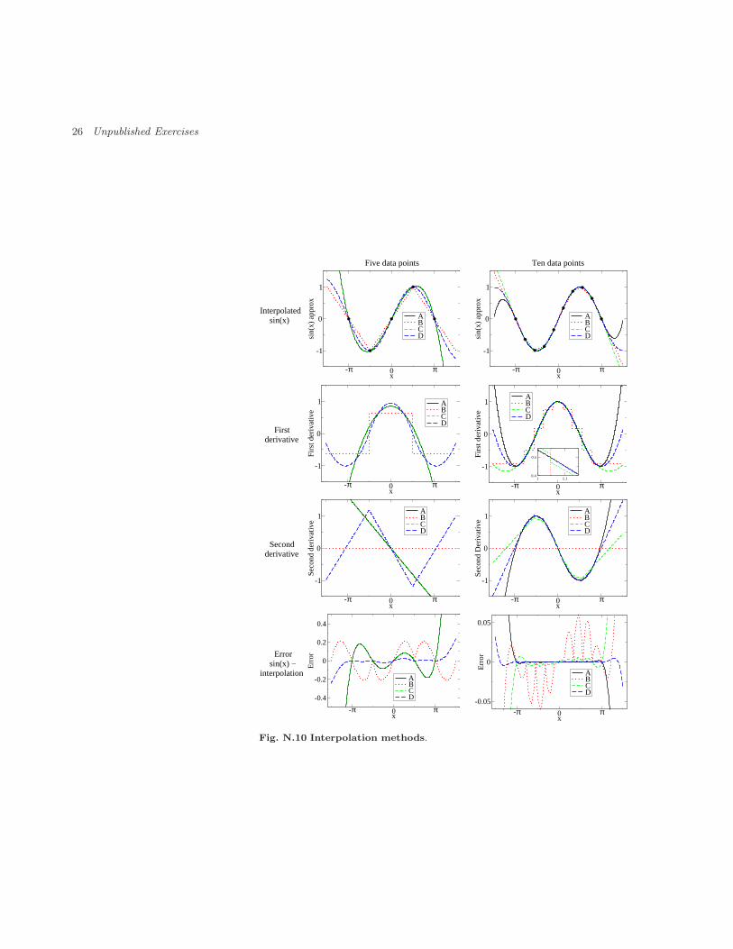
26 Unpublished Exercises
interpolation
-π 0 πx
-1
0
1
Firs
t der
ivat
ive
ABCD
-π 0 πx
-1
0
1
Seco
nd d
eriv
ativ
e
ABCD
-π 0 πx
-0.4
-0.2
0
0.2
0.4
Err
or
ABCD
-π 0 πx
-1
0
1
sin(
x) a
ppro
x
ABCD
-π 0 πx
-1
0
1
Firs
t der
ivat
ive
ABCD
1 1.10.4
0.5
-π 0 πx
-1
0
1
Seco
nd D
eriv
ativ
e
ABCD
-π 0 πx
-0.05
0
0.05
Err
or
ABCD
Five data points Ten data points
Interpolatedsin(x)
Firstderivative
Secondderivative
Errorsin(x) −
-π 0 πx
-1
0
1
sin(
x) a
ppro
xABCD
Fig. N.10 Interpolation methods.
Exercises 27
periodic boundary conditions, the end-points areno longer special. What corresponds to Gaus-sian quadrature for periodic functions is justthe trapezoidal rule: equally-weighted points atequally spaced intervals.
(N.25) Numerical derivatives. (Rounding errors,Accuracy) ©2Calculate the numerical first derivative of thefunction y(x) = sin(x), using the centered two-point formula dy/dx ∼ (y(x+h)−y(x−h))/(2h),and plot the error y′(x) − cos(x) in the range(−π, π) at 100 points. (Do a good job! Use thestep-size h described in section 5.7 to optimizethe sum of the truncation error and the round-ing error. Also, make sure that the step-size his exactly representable on the machine.) Howdoes your actual error compare to the fractionalerror estimate given in section 5.7? Calculateand plot the numerical second derivative usingthe formula
d2y
dx2∼ y(x + h) − 2y(x) + y(x − h)
h2, (N.50)
again optimizing h and making it exactly repre-sentable. Estimate your error again, and com-pare to the observed error.
(N.26) Summing series. (Efficiency) ©2Write a routine to calculate the sum
sn =
nX
j=0
(−1)j 1
2j + 1. (N.51)
As n → ∞, s∞ = π/4. About how many termsdo you need to sum to get convergence to within10−7 of this limit? Now try using Aitken’s ∆2
process to accelerate the convergence:
s′n = sn − (sn+1 − sn)2
sn+2 − 2sn+1 + sn. (N.52)
About how many terms do you need with Aitken’smethod to get convergence to within 10−7?
(N.27) Random histograms. (Random numbers) ©2
(a) Investigate the random number generator foryour system of choice. What is its basic algo-rithm? Its period?(b) Plot a histogram with 100 bins, giving thenormalized probability density of 100,000 ran-dom numbers sampled from (a) a uniform dis-tribution in the range 0 < x < 2π, (b) an ex-ponential distribution ρ(x) = 6 exp(−6x), and(c) a normal distribution of mean x = 3π/2 and
standard deviation σ = 1/√
6. Before each plot,set the seed of your random number generator.Do you now get the same plot when you repeat?
(N.28) Monte Carlo integration. (Random num-bers, Robust algorithms) ©3How hard can numerical integration be? Sup-pose the function f is wildly nonanalytic, or hasa peculiar or high-dimensional domain of inte-gration? In the worst case, one can always tryMonte Carlo integration. The basic idea is topepper points at random in the integration in-terval. The integration volume times the averageof the function V 〈f〉 is the estimate of the inte-gral.As one might expect, the expected error inthe integral after N evaluations is given by1/
√N − 1 times the standard deviation of the
sampled points (NR equation 7.7.1).(a) Monte Carlo in one dimensional integrals.Use Monte Carlo integration to estimate the in-tegral of the function introduced in the prelimi-nary exercises
y(x) = exp(−6 sin(x)) (N.53)
over 0 ≤ x < 2π. (The correct value of the inte-gral is around 422.446.) How many points do youneed to get 1% accuracy? Answer this last ques-tion both by experimenting with different randomnumber seeds, and by calculating the expectednumber from the standard deviation. (You mayuse the fact that 〈y2〉 = (1/2π)
R 2π
0y2(x)dx ≈
18948.9.)Monte Carlo integration is not the most efficientmethod for calculating integrals of smooth func-tions like y(x). Indeed, since y(x) is periodicin the integration interval, equally spaced pointsweighted equally (the trapezoidal rule) gives ex-ponentially rapid convergence; it takes only ninepoints to get 1% accuracy. Even for smoothfunctions, though, Monte Carlo integration isuseful in high dimensions.(b) Monte Carlo in many dimensions (No de-tailed calculations expected). For a hypotheti-cal ten-dimensional integral, if we used a regulargrid with nine points along each axis, how manyfunction evaluations would we need for equiva-lent accuracy? Does the number of Monte Carlopoints needed depend on the dimension of thespace, presuming (perhaps naively) that the vari-ance of the function stays fixed?Our function y(x) is quite close to a Gaussian.(Why? Taylor expand sin(x) about x = 3π/2.)
28 Unpublished Exercises
We can use this to do importance sampling. Theidea is to evaluate the integral of h(x)g(x) byrandomly sampling h with probability g, pick-ing h(x) = y(x)/g(x). The variance is then〈h2〉 − 〈h〉2. In order to properly sample the tailnear x = π/2, we should mix a Gaussian and auniform distribution:
g(x) =ǫ
2π+
1 − ǫp
π/3exp(−6(x − 3π/2)2/2).
(N.54)I found minimum variance around ǫ = 0.005.(c) Importance Sampling (Optional for 480).Generate 1000 random numbers with probabilitydistribution g.39 Use these to estimate the inte-gral of y(x). How accurate is your answer?
(N.29) The Birthday Problem. (Sorting, Randomnumbers) ©2Remember birthday parties in your elementaryschool? Remember those years when two kidshad the same birthday? How unlikely!How many kids would you need in class to get,more than half of the time, at least two with thesame birthday?(a) Numerical. Write a routineBirthdayCoincidences(K, C) that returns thefraction among C classes for which at least twokids (among K kids per class) have the samebirthday. (Hint: By sorting a random list of in-tegers, common birthdays will be adjacent.) Plotthis probability versus K for a reasonably largevalue of C. Is it a surprise that your classes hadoverlapping birthdays when you were young?One can intuitively understand this, by remem-bering that to avoid a coincidence there areK(K − 1)/2 pairs of kids, all of whom musthave different birthdays (probability 364/365 =1 − 1/D, with D days per year).
P (K, D) ≈ (1 − 1/D)K(K−1)/2 (N.55)
This is clearly a crude approximation – it doesn’tvanish if K > D! Ignoring subtle correlations,though, it gives us a net probability
P (K,D) ≈ exp(−1/D)K(K−1)/2
≈ exp(−K2/(2D)) (N.56)
Here we’ve used the fact that 1 − ǫ ≈ exp(−ǫ),and assumed that K/D is small.(b) Analytical. Write the exact formula givingthe probability, for K random integers among Dchoices, that no two kids have the same birthday.(Hint: What is the probability that the secondkid has a different birthday from the first? Thethird kid has a different birthday from the firsttwo?) Show that your formula does give zero ifK > D. Converting the terms in your product toexponentials as we did above, show that your an-swer is consistent with the simple formula above,if K ≪ D. Inverting equation N.56, give a for-mula for the number of kids needed to have a 50%chance of a shared birthday.Some years ago, we were doing a large simula-tion, involving sorting a lattice of 10003 randomfields (roughly, to figure out which site on thelattice would trigger first). If we want to makesure that our code is unbiased, we want differ-ent random fields on each lattice site – a giantbirthday problem.Old-style random number generators generateda random integer (232 ‘days in the year’) andthen divided by the maximum possible integerto get a random number between zero and one.Modern random number generators generate all252 possible doubles between zero and one.(c) If there are 231 − 1 distinct four-byte posi-tive integers, how many random numbers wouldone have to generate before one would expect co-incidences half the time? Generate lists of thatlength, and check your assertion. (Hints: It isfaster to use array operations, especially in in-terpreted languages. I generated a random ar-ray with N entries, sorted it, subtracted the firstN−1 entries from the last N−1, and then calledmin on the array.) Will we have to worry aboutcoincidences with an old-style random numbergenerator? How large a lattice L × L × L ofrandom double precision numbers can one gener-ate with modern generators before having a 50%chance of a coincidence? If you have a fast ma-chine with a large memory, you might test thistoo.
39Take (1 − ǫ)M Gaussian random numbers and ǫM random numbers uniformlydistributed on (0, 2π). The Gaussian has a small tail that extends beyond the inte-gration range (0, 2π), so the normalization of the second term in the definition of g isnot quite right. You can fix this by simply throwing away any samples that includepoints outside the range.
Exercises 29
(N.30) Washboard Potential. (Solving) ©2Consider a washboard potential40
V (r) = A1 cos(r) + A2 cos(2r) − Fr (N.57)
with A1 = 5, A2 = 1, and F initially equal to1.5.(a) Plot V (r) over (−10, 10). Numerically findthe local maximum of V near zero, and the localminimum of V to the left (negative side) of zero.What is the potential energy barrier for movingfrom one well to the next in this potential?Usually finding the minimum is only a first step– one wants to explore how the minimum movesand disappears. . .(b) Increasing the external tilting field F , graph-ically roughly locate the field Fc where the barrierdisappears, and the location rc at this field wherethe potential minimum and maximum merge.(This is a saddle-node bifurction.) Give thecriterion on the first derivative and the secondderivative of V (r) at Fc and rc. Using these twoequations, numerically use a root-finding routineto locate the saddle-node bifurcation Fc and rc.
(N.31) Sloppy Minimization. (Minimization) ©3“With four parameters I can fit an elephant.With five I can make it waggle it’s trunk.” Thisstatement, attributed to many different sources(from Carl Friedrich Gauss to Fermi), reflects theproblems found in fitting multiparameter modelsto data. One almost universal problem is slop-piness – the parameters in the model are poorlyconstrained by the data.41
Consider the classic ill-conditioned problem offitting exponentials to radioactive decay data. Ifyou know that at t = 0 there are equal quantitiesof N radioactive materials with half-lives γn, theradioactivity that you would measure is
y(t) =
N−1X
n=0
γn exp(−γnt). (N.58)
Now, suppose you don’t know the decay rates γn.Can you reconstruct them by fitting the data toexperimental data y0(t)?
Let’s consider the problem with two radioactivedecay elements N = 2. Suppose the actual de-cay constants for y0(t) are αn = n + 2 (so theexperiment has γ0 = α0 = 2 and γ1 = α1 = 3),and we try to minimize the least-squared error42
in the fits C:
C[γ ] =
Z ∞
0
(y(t) − y0(t))2 dt. (N.59)
You can convince yourself that the least-squarederror is
C[γ] =N−1X
n=0
N−1X
m=0
“ γnγm
γn + γm
+αnαm
αn + αm− 2
γnαm
γn + αm
”
=49
10+
γ0
2− 4 γ0
2 + γ0− 6 γ0
3 + γ0
+γ1
2− 4 γ1
2 + γ1− 6 γ1
3 + γ1+
2 γ0 γ1
γ0 + γ1.
(a) Draw a contour plot of C in the square1.5 < γn < 3.5, with enough contours (perhapsnon-equally spaced) so that the two minima canbe distinguished. (You’ll also need a fairly finegrid of points.)One can see from the contour plot that measur-ing the two rate constants separately would be achallenge. This is because the two exponentialshave similar shapes, so increasing one decay rateand decreasing the other can almost perfectlycompensate for one another.(b) If we assume both elements decay with thesame decay constant γ = γ0 = γ1, minimize thecost to find the optimum choice for γ. Whereis this point on the contour plot? Plot y0(t) andy(t) with this single-exponent best fit on the samegraph, over 0 < t < 2. Do you agree that it wouldbe difficult to distinguish these two fits?This problem can become much more severe inhigher dimensions. The banana-shaped ellipsesin your contour plot can become needle-like, withaspect ratios of more than a thousand to one(about the same as a human hair). Followingthese thin paths down to the true minima can
40A washboard is what people used to hand-wash clothing. It is held at an angle,and has a series of corrugated ridges; one holds the board at an angle and rubsthe wet clothing on it. Washboard potentials arise in the theory of superconductingJosephson junctions, in the motion of defects in crystals, and in many other contexts.41‘Elephantness’ says that a wide range of behaviors can be exhibited by varyingthe parameters over small ranges. ‘Sloppiness’ says that a wide range of parameterscan yield approximately the same behavior. Both reflect a skewness in the relationbetween parameters and model behavior.42We’re assuming perfect data at all times, with uniform error bars.
30 Unpublished Exercises
be a challenge for multidimensional minimiza-tion programs.(c) Find a method for storing and plottingthe locations visited by your minimization rou-tine (values of (γ0, γ1) at which it evaluatesC while searching for the minimum). Startingfrom γ0 = 1, γ1 = 4, minimize the cost us-ing as many methods as is convenient withinyour programming environment, such as Nelder-Mead, Powell, Newton, Quasi-Newton, conju-gate gradient, Levenberg-Marquardt (nonlinearleast squares). . . . (Try to use at least one thatdoes not demand derivatives of the function).Plot the evaluation points on top of the contourplot of the cost for each method. Compare thenumber of function evaluations needed for thedifferent methods.
(N.32) Sloppy Monomials.43 (Eigenvalues, Fit-ting) ©3We have seen that the same function f(x) canbe approximated in many ways. Indeed, thesame function can be fit in the same intervalby the same type of function in several differ-ent ways! For example, in the interval [0, 1], thefunction sin(2πx) can be approximated (badly)by a fifth-order Taylor expansion, a Chebyshevpolynomial, or a least-squares (Legendre44 ) fit:
f(x) = sin(2πx)
≈ 0.000 + 6.283x + 0.000x2 − 41.342x3
+ 0.000x4 + 81.605x5 Taylor
≈ 0.007 + 5.652x + 9.701x2 − 95.455x3
+ 133.48x4 − 53.39x5 Chebyshev
≈ 0.016 + 5.410x + 11.304x2 − 99.637x3
+ 138.15x4 − 55.26x5 Legendre
It is not a surprise that the best fit polynomialdiffers from the Taylor expansion, since the lat-ter is not a good approximation. But it is asurprise that the last two polynomials are so dif-ferent. The maximum error for Legendre is lessthan 0.02, and for Chebyshev is less than 0.01,
even though the two polynomials differ by
Chebyshev − Legendre = (N.60)
− 0.009 + 0.242x − 1.603x2
+ 4.182x3 − 4.67x4 + 1.87x5
a polynomial with coefficients two hundred timeslarger than the maximum difference!This flexibility in the coefficients of the polyno-mial expansion is remarkable. We can study itby considering the dependence of the quality ofthe fit on the parameters. Least-squares (Legen-dre) fits minimize a cost CLeg, the integral of thesquared difference between the polynomial andthe function:
CLeg = (1/2)
Z 1
0
(f(x) −M
X
m=0
amxm)2 dx.
(N.61)How quickly does this cost increase as we movethe parameters am away from their best-fit val-ues? Varying any one monomial coefficient willof course make the fit bad. But apparentlycertain coordinated changes of coefficients don’tcost much – for example, the difference be-tween least-squares and Chebyshev fits given ineqn (N.60).How should we explore the dependence in arbi-trary directions in parameter space? We can usethe eigenvalues of the Hessian to see how sensi-tive the fit is to moves along the various eigen-vectors. . .(a) Note that the first derivative of the cost CLeg
is zero at the best fit. Show that the Hessian sec-ond derivative of the cost is
HLegmn =
∂2CLeg
∂am∂an=
1
m + n + 1. (N.62)
This Hessian is the Hilbert matrix, famous forbeing ill-conditioned (having a huge range ofeigenvalues). Tiny eigenvalues of HLeg corre-spond to directions in polynomial space wherethe fit doesn’t change.(b) Calculate the eigenvalues of the 6×6 Hessianfor fifth-degree polynomial fits. Do they span alarge range? How big is the condition number?(c) Calculate the eigenvalues of larger Hilbertmatrices. At what size do your eigenvalues seem
43Thanks to Joshua Waterfall, whose research is described here.44The orthogonal polynomials used for least-squares fits on [-1,1] are the Legendrepolynomials, assuming continuous data points. Were we using orthogonal polynomi-als for this exercise, we would need to shift them for use in [0,1].
Exercises 31
contaminated by rounding errors? Plot them, inorder of decreasing size, on a semi-log plot toillustrate these rounding errors.Notice from Eqn N.62 that the dependence of thepolynomial fit on the monomial coefficients is in-dependent of the function f(x) being fitted. Wecan thus vividly illustrate the sloppiness of poly-nomial fits by considering fits to the zero func-tion f(x) ≡ 0. A polynomial given by an eigen-vector of the Hilbert matrix with small eigen-value must stay close to zero everywhere in therange [0, 1]. Let’s check this.(d) Calculate the eigenvector corresponding tothe smallest eigenvalue of HLeg, checking tomake sure its norm is one (so the coefficients areof order one). Plot the corresponding polynomialin the range [0, 1]: does it stay small everywherein the interval? Plot it in a larger range [−1, 2]to contrast its behavior inside and outside the fitinterval.This turns out to be a fundamental propertythat is shared with many other multiparame-ter fitting problems. Many different terms areused to describe this property. The fits arecalled ill-conditioned: the parameters an are notwell constrained by the data. The inverse prob-lem is challenging: one cannot practically ex-tract the parameters from the behavior of themodel. Or, as our group describes it, the fit issloppy: only a few directions in parameter space(eigenvectors corresponding to the largest eigen-values) are constrained by the data, and thereis a huge space of models (polynomials) varyingalong sloppy directions that all serve well in de-scribing the data.At root, the problem with polynomial fits isthat all monomials xn have similar shapes on[0, 1]: they all start flat near zero and bendupward. Thus they can be traded for one an-other; the coefficient of x4 can be lowered with-out changing the fit if the coefficients of x3 andx5 are suitably adjusted to compensate. Indeed,if we change basis from the coefficients an of themonomials xn to the coefficients ℓn of the orthog-onal (shifted Legendre) polynomials, the situa-tion completely changes. The Legendre polyno-mials are designed to be different in shape (or-thogonal), and hence cannot be traded for oneanother. Their coefficients ℓn are thus well de-
termined by the data, and indeed the Hessian forthe cost CLeg in terms of this new basis is theidentity matrix.Numerical Recipes states a couple of times thatusing equally-spaced points gives ill-conditionedfits. Will the Chebyshev fits, which emphasizethe end-points of the interval, give less sloppy co-efficients? The Chebyshev polynomial for a func-tion f (in the limit where many terms are kept)minimizes a different cost: the squared differenceweighted by the extra factor 1/
p
x(1 − x):
CCheb =
Z 1
0
(f(x) − PMm=0 cmxm)2
p
x(1 − x)dx.
(N.63)One can show that the Hessian giving the depen-dence of CCheb on cm is
HChebmn =
∂2CCheb
∂cm∂cn=
21−2(m+n)π(2(m + n) − 1)!
(m + n − 1)!(m + n)!.
(N.64)with HCheb
00 = π (doing the integral explicitly, ortaking the limit m, n → 0).(d) (Optional for 480) Calculate the eigenvaluesof HCheb for fifth-degree polynomial fits.So, sloppiness is not peculiar to least-squares fits;Chebyshev polynomial coefficients are sloppytoo.
(N.33) Conservative differential equations: Accu-
racy and fidelity. (Ordinary differential equa-tions) ©3In this exercise, we will solve for the motion of aparticle of mass m = 1 in the potential
V (y) = (1/8) y2(−4A2 + log2(y2)). (N.65)
That is,
d2y/dt2 = −dV/dy (N.66)
= −(1/4)y(−4A2 + 2 log(y2) + log2(y2)).
We will start the particle at y0 = 1, v0 =dy/dt|0 = −A, and choose A = 6.(a) Show that the solution to this differentialequation is45
F (t) = exp(−6 sin(t)). (N.67)
Note that the potential energy V (y) is zero atthe five points y = 0, y = ± exp(±A).(b) Plot the potential energy for−3/2 exp(±A) < y < 3/2 exp(±A) (both zoomed
45I worked backward to do this. I set the kinetic energy to 1/2(dF/dt)2 , set thepotential energy to minus the kinetic energy, and then substituted y for t by solvingy = F (t).
32 Unpublished Exercises
in near y = 0 and zoomed out). The correcttrajectory should oscillate in the potential wellwith y > 0, turning at two points whose energyis equal to the initial total energy. What is thisinitial total energy for our the particle? Howmuch of an error in the energy would be needed,for the particle to pass through the origin whenit returns? Compare this error to the maximumkinetic energy of the particle (as it passes thebottom of the well). Small energy errors in ourintegration routine can thus cause significantchanges in the trajectory.(c) (Black-box) Using a professionally writtenblack-box differential equation solver of yourchoice, solve for y(t) between zero and 4π, athigh precision. Plot your answer along with F (t)from part (a). (About half of the solvers will getthe answer qualitatively wrong, as expected frompart (b).) Expand your plot to examine the re-gion 0 < y < 1; is energy conserved? Finally,read the documentation for your black box rou-tine, and describe the combination of algorithmsbeing used. You may wish to implement andcompare more than one algorithm, if your black-box has that option.
Choosing an error tolerance for your differentialequation limits the error in each time step. Ifsmall errors in early time steps lead to impor-tant changes later, your solution may be quitedifferent from the correct one. Chaotic motion,for example, can never be accurately simulatedon a computer. All one can hope for is a faithfulsimulation – one where the motion is qualita-tively similar to the real solution. Here we findan important discrepancy – the energy of the nu-merical solution is drifting upward or downward,where energy should be exactly conserved in thetrue solution. Here we get a dramatic change inthe trajectory for a small quantitative error, butany drift in the energy is qualitatively incorrect.The Leapfrog algorithm is a primitive lookingmethod for solving for the motion of a particlein a potential. It calculates the next positionfrom the previous two:
y(t + h) = 2y(t) − y(t − h) + h2f [y(t)] (N.68)
where f [y] = −dV/dy. Given an initial positiony(0) and an initial velocity v(0), one can initial-
ize and finalize
y(h) = y(0) + h(v(0) + (h/2)f [y(0)])
v(T ) = (y(T )− y(T − h))/h + (h/2)f [y(T )](N.69)
Leapfrog is one of a variety of Verlet algorithms.In a more general context, this is called Sto-ermer’s rule, and can be extrapolated to zerostep-size h as in the Bulirsch–Stoer algorithms.A completely equivalent algorithm, with morestorage but less roundoff error, is given by com-puting the velocity v at the midpoints of eachtime step:
v(h/2) = v(0) + (h/2)f [y(0)]
y(h) = y(0) + h v(h/2)
v(t + h/2) = v(t − h/2) + hf [y(t)]
y(t + h) = y(t) + h v(t + h/2)
(N.70)
where we may reconstruct v(t) at integer timesteps with v(t) = v(t − h/2) + (h/2)f [y(t)].(d) (Leapfrog and symplectic methods) Showthat y(t + h) and y(h) from eqns N.68 and N.69converge to the true solutions as as h → 0 –that is, the time-step error compared to the so-lution of d2y/dt2 = f [y] vanishes faster than h.To what order in h are they accurate after onetime step?46 Implement Leapfrog, and apply it tosolving equation N.66 in the range 0 < x < 4π,starting with step size h = 0.01. How does theaccuracy compare to your more sophisticated in-tegrator, for times less than t = 2? Zoom into the range 0 < y < 1, and compare with yourpackaged integrator and the true solution. Whichhas the more accurate period (say, by measuringthe time to the first minimum in y)? Which hasthe smaller energy drift (say, by measuring thechange in depth between subsequent minima)?
Fidelity is often far more important than accu-racy in numerical simulations. Having an al-gorithm that has a small time-step error butgets the behavior qualitatively wrong is less use-ful than a cruder answer that is faithful to thephysics. Leapfrog here is capturing the oscillat-ing behavior far better than vastly more sophisti-cated algorithms, even though it gets the periodwrong.How does Leapfrog do so well? Systems likeparticle motion in a potential are Hamiltonian
46Warning: for subtle reasons, the errors in Leapfrog apparently build up quadrati-cally as one increases the number of time steps, so if your error estimate after one timestep is hn the error after N = T/h time steps can’t be assumed to be Nhn ∼ hn−1,but is actually N2hn ∼ hN−2.
Exercises 33
systems. They not only conserve energy, butthey also have many other striking propertieslike conserving phase-space volume (Liouville’stheorem, the basis for statistical mechanics).Leapfrog, in disguise, is also a Hamiltonian sys-tem. (Eqns N.70 can be viewed as a compositionof two canonical transformations – one advanc-ing the velocities at fixed positions, and one ad-vancing the positions at fixed velocities.) Henceit exactly conserves an approximation to the en-ergy – and thus doesn’t suffer from energy drift,satisfies Liouville’s theorem, etc. Leapfrog and
the related Verlet algorithm are called symplecticbecause they conserve the symplectic form thatmathematicians use to characterize Hamiltoniansystems.It is often vastly preferable to do an exact sim-ulation (apart from rounding errors) of an ap-proximate system, rather than an approximateanalysis of an exact system. That way, one canknow that the results will be physically sensible(and, if they are not, that the bug is in yourmodel or implementation, and not a feature ofthe approximation).


References
[1] Buchel, A. and Sethna, J. P. (1996). Elastic theory has zero radiusof convergence. Physical Review Letters , 77, 1520.
[2] Buchel, A. and Sethna, J. P. (1997). Statistical mechanicsof cracks: Thermodynamic limit, fluctuations, breakdown, andasymptotics of elastic theory. Physical Review E , 55, 7669.
[3] Davies, C. T. H., Follana, E., Gray, A., Lepage, G. P., and et al.(2004). High-precision lattice qcd confronts experiment. PhysicalReview Letters , 92, 022001.
[4] Dyson, Freeman (1960). Search for artificial stellar sources of in-frared radiation. Science, 131, 1667–1668.
[5] Mezard, M. and Montanari, A. (To be published (2006)). Con-straint satisfaction networks in Physics and Computation. Claren-don Press, Oxford.
[6] Otani, N. (2004). Home page. http://otani.vet.cornell.edu.[7] Sethna, J. P. (1997). Quantum electro-
dynamics has zero radius of convergence.http://www.lassp.cornell.edu/sethna/Cracks/QED.html.
[8] Sethna, J. P. and Myers, C. R. (2004). Entropy, Order Param-eters, and Complexity computer exercises: Hints and software.http://www.physics.cornell.edu/sethna/StatMech/ComputerExercises.html.
[9] Skriver, H. (2004). The hls metals database.http://http://databases.fysik.dtu.dk/hlsPT/.
[10] Smith, R. L. (To be published (2006)). Environmental Statistics.[11] Winfree, A. T. (1991). Varieties of spiral wave behavior: An exper-
imentalist’s approach to the theory of excitable media. Chaos , 1,303–34.
[12] Zinn-Justin, J. (1996). Quantum field theory and critical phenom-ena (3rd edition). Oxford University Press.