An introduction to entropy estimation of parameters in

ENTROPY ESTIMATION OF PARAMETERS IN ECONOMIC MODELS 1

An introduction to entropy estimation of parameters in economic models

Larry Cook and Philip Harslett*

The results from quantitative economic modelling are highly dependent on the parameter values that are adopted. Where modellers lack the data to make their own reliable estimates, which is often the case for elasticities, a common practice is to use elasticity values from previous modelling. In some cases assumed or stylised values are used, in others the values can be traced back to one or more econometric studies.

While borrowing elasticities is a sensible starting point in any modelling exercise, users are left in doubt as to whether elasticities from other times and places, that use different aggregations or are based on longer or shorter periods of adjustment, are applicable for the current exercise. It therefore puts the robustness of results in doubt. However, using conventional econometric methods to estimate parameters is not an option when data are limited, as is often the case with the economic variables required for CGE models. Hence the modeller is left with the problem of determining the most suitable parameters.

Entropy estimation, developed by Golan, Judge and Miller (1996), is an approach that allows economic modellers to use data to improve the assumptions they make about parameters in economic models. It works by using prior information — a combination of past estimates, educated guesses, and theoretical constraints — and limited data to inform estimates. Importantly, entropy estimation places more weight on the data (and less on the priors) as the number of observations increase. A further attraction is that the resulting entropy parameter estimates must satisfy the underlying economic model equations since those equations are constraints in the entropy estimation.

While entropy estimation has the potential to improve the quality of parameters used in policy analysis, and thus the confidence in conclusions from economic modelling, its use has not been widespread. Most applications have been to single or multi equation demand systems, but in a few noteworthy cases elasticity estimates have been made with full general equilibrium constraints (Arndt, Robinson and Tarp 2002; Liu, Arndt and Hertel 2000; Go, Lofgren, Mendez Ramos and Robinson 2014).

The purpose of this short paper is to provide an introductory guide to entropy estimation for economic modellers with a particular emphasis on estimating elasticities from limited time series data. The objective is to provide all the information that researchers need (how it works, the importance of the assumptions, and when and how it should be used) to be able to use the technique confidently.

2 CONFERENCE PAPER

* Paper to be presented at the 18th Annual Conference on Global Economic Analysis, Melbourne, June 17-19, 2015. Australian Productivity Commission. The authors are grateful for comments from Professor Paul Preckel, Tim Murray and Patrick Jomini on earlier drafts. Any errors or omissions remain the authors’ responsibility.


1 Introduction

The results from quantitative economic modelling are highly dependent on the parameter values that are adopted. Elasticities measuring behavioural responses are particularly problematic given that there is generally a high degree of uncertainty surrounding their values. A common practice is to use elasticity values from previous modelling, which in some cases are simply assumed or stylised values, or can be traced back to econometric studies.

While borrowing elasticities is a sensible starting point in any modelling exercise, users are left in doubt as to whether the elasticities from other times and places, that use different aggregations or are based on longer or shorter periods of adjustment, are applicable for the current exercise. It therefore puts the robustness of results in doubt and, for this reason, it is always good modelling practice to do extensive sensitivity testing and provide ranges for results based on different elasticities and other parameters.

While the preferred approach is to estimate parameters using current relevant data, the difficulties are often considerable. All too commonly economic data are limited and noisy, especially the data needed to estimated parameters in disaggregated computable general equilibrium (CGE) models. With problematic piecemeal data, short time series, and possible simultaneity issues, parameter estimates based on conventional econometric estimation methods may deviate significantly from their true values and may even be implausible.

Entropy econometrics developed by Golan, Judge and Miller (1996) offers a useful approach for improving the assumptions made about parameters in economic models. As a starting point, it takes prior information — whether from previous studies, theory, or educated guesses — in the form of a probability distribution. Entropy econometrics then determines how these prior probabilities should be improved in the light of available data and constraints. With few observations, the estimated probabilities generally will be close to the priors, but as more observations of real-world data become available, the probabilities will be more reflective of the additional information in the data and depend less on the priors. A feature of entropy estimation as applied to model parameters is that the model equations form part of the information base for improving the estimates. This has the advantage of ensuring that the model parameters are consistent.

Although entropy econometrics has been used to estimate elasticities from time series its use has not been widespread. Most applications have been to single or multi equation demand systems (Fraser 2000; Golan, Perloff and Shen 2001; Balcombe, Rapsomanikis and Klonaris 2004; Nganou 2004; Nunez 2009; Joshi, Hanrahan, Murphy and Kelley 2010), but in several noteworthy cases elasticity estimates have been made with full general equilibrium constraints (Arndt, Robinson and Tarp 2001; Go et al. 2014; Liu, Arndt and Hertel 2000).

4 CONFERENCE PAPER

A more generally recognised use of entropy techniques has been in constructing the input-output and social accounting matrices that underlie computable general equilibrium (CGE) modelling (McDougall 1999; Golan and Vogel 2000; Golan, Judge and Robinson 2001; Robinson, Cattaneo and El-Said 2001; Ahmed and Preckel 2007). Indeed, this is the only use of entropy that is referred to in the comprehensive two volume Handbook of Computable General Equilibrium Modeling (Dixon and Jorgenson 2012).

Outside of GCE modelling, entropy techniques have been applied to the calibration of environmental and agricultural policy models (Howitt and Msangi 2006; Howitt and Reynaud 2003; Howitt 2005; Paris and Howitt 1998).

The purpose of this paper is to provide an introductory guide to entropy estimation for economic modellers with a particular emphasis on estimating elasticities from time series. The objective is to provide all the information that modellers need (how it works, the importance of the assumptions, and when and how it should be used) to be able to use the technique confidently.

Section 2 starts with the cross entropy function and illustrates how minimising cross entropy subject to known constraints can be used to solve undetermined problems where there are more unknowns than equations. The classic example first discussed is Jaynes (1963) die problem, followed by some simple examples of how the method is used in the estimation of accounting matrices and model calibration.

Section 3 describes how cross entropy is used to estimate elasticities from time series in the simplest case of a single equation, and the importance of the underlying assumptions when there are few observations. Monte Carlo simulations are undertaken to compare the distributions of ordinary least squares and entropy estimators when data are limited. This illustrates under what circumstances entropy estimation is likely to be preferable to traditional econometric estimators based on the characteristic of the available data and the assumptions that have to be made about priors.

Section 4 explains the application of the technique to estimating elasticities from time series data to where the model involves simultaneous equations. Monte Carlo simulations are used to test for the consistency of different estimators and their effectiveness with small samples.

Section 5 provides concluding remarks.

An appendix contains a listing of GAMS computer code that is the basis for the entropy elasticity estimates in the examples in this paper.


2 Using cross entropy for undetermined problems

2.1 The cross entropy function

The Kullback-Liebler measure of cross entropy measures the difference between two probability distributions. The discrete form of this function is:

(2.1) CE = ∑𝜋𝜋𝑗 ∙ 𝑙𝑛�𝜋𝜋𝑗 𝜋𝜋𝑗′⁄ �

where 𝜋𝜋𝑗 is the probability of the jth outcome occurring for the first probability distribution and 𝜋𝜋𝑗′ is the probability of the jth outcome occurring for the second probability distribution. The cross entropy function is equal to zero when 𝜋𝜋𝑗 is equal to 𝜋𝜋𝑗′ for all values of j. The greater the value of the cross entropy function, the larger is the difference between the two probability distributions. As pointed out by Preckel (2001) cross entropy can be interpreted as a penalty function over deviations between two distributions. This is most easily seen by noting that (Golan, Judge and Miller 1996, p. 31).

(2.2) CE ≈ ∑ 1𝜋𝑗∙ �𝜋𝜋𝑗 − 𝜋𝜋𝑗′�

2

An illustrative example of the cross entropy measure between a uniform probability distribution 𝜋𝜋𝑗′ and several other probability distributions 𝜋𝜋𝑗𝑘 is given in table 2.1.

Table 2.1 Kullback Liebler measure of cross entropy

Outcome (j)

Probabilities (𝜋𝜋𝑗′)

Probabilities (𝜋𝜋𝑗)

𝜋𝜋𝑗1 𝜋𝜋𝑗2 𝜋𝜋𝑗3 𝜋𝜋𝑗4

1 0.167 0.16 0 0.1 0.054 2 0.167 0.16 0 0.1 0.079 3 0.167 0.16 0 0.1 0.114 4 0.167 0.16 0.5 0.1 0.165 5 0.167 0.18 0.5 0.1 0.240 6 0.167 0.18 0 0.5 0.347 Sum 1.0 1.0 1.0 1.0 1.0 𝐶𝐸 =∑𝜋𝜋𝑗 ∙ 𝑙𝑛�𝜋𝜋𝑗 𝜋𝜋𝑗′⁄ � - 0.002 1.098 0.294 0.177

𝑁𝑜𝑡𝑒𝑒: ∑ 𝜋𝜋𝑗 𝑗𝑗 3.5 3.6 4.5 4.5 4.5

Notice that all distributions in this table satisfy the condition that the probabilities sum to unity, but that the distributions that are ‘closest’ to 𝜋𝜋𝑗′ (such as 𝜋𝜋𝑗1) have smaller CE values and those that are more different (such as 𝜋𝜋𝑗2) have larger CE values.

6 CONFERENCE PAPER

2.2 Estimation of a probability distribution subject to constraints: Jaynes’ die problem

(Jaynes 1963, pp. 183-187) posed the following problem: ‘A die has been tossed a very large number N of times, and we are told that the average number of spots per toss was not 3.5, as we might expect from an honest die, but 4.5. Translate this information into a probability assignment 𝜋𝜋𝑗, j = 1, 2,…, 6, for the j-th face to come up on the next toss.’ [notation changed]

As Jaynes pointed out, a possible solution would be 𝜋𝜋4 = 𝜋𝜋5 = 0.5 and all other 𝜋𝜋𝑗 = 0 (the 𝜋𝜋𝑗2 distribution in table 2.1) but that does not seem a reasonable assignment since nothing in the data tells us that events other than 4 and 5 are impossible. Rather,

‘A reasonable assignment 𝜋𝜋𝑗 must not only agree with the data and must not ignore any possibility - but it must also not give undue emphasis to any possibility.’

(for example the 𝜋𝜋𝑗3 distribution in table 2.1 gives undue emphasis to 6). Jaynes concluded that,

‘The probability assignment πj which most honestly describes what we know is the one that is as smooth and “spread out” as possible subject to the data. It is the most conservative assignment in the sense that it does not permit one to draw any conclusions not warranted by the data.’

and,

‘we need a measure of the “spread” of a probability distribution which we can maximize, subject to constraints which represent the available information.’

As Jaynes went on to point out, the correct measure of the spread is Shannon's (1948) entropy measure. And since in this case the prior probability distribution is uniform, then maximising Shannon’s entropy is equivalent to minimising the cross entropy between the prior and estimated probabilities.1

Thus Jaynes’ solution to the die problem with given prior probabilities 𝜋𝜋1′ = ⋯ = 𝜋𝜋6′ = 0.167, can be determined by choosing 𝜋𝜋1 …𝜋𝜋6 to minimise:

(2.3) 𝐶𝐸 = ∑𝜋𝜋𝑗 ∙ 𝑙𝑛�𝜋𝜋𝑗 𝜋𝜋𝑗′⁄ �

1 A special case of (2.1) is when one of the distributions is uniform, e.g. when 𝜋𝜋𝑗′=1/n for all j=1,…, n. In

this case:

CE = ∑𝜋𝜋𝑗 ∙ 𝑙𝑛 �𝜋𝜋𝑗1n⁄ �,

= 𝑙𝑛(n) —∑𝜋𝜋𝑗 ∙ 𝑙𝑛�𝜋𝜋𝑗�

= 𝑙𝑛(n) − 𝐸 where E is Shannon’s measure of entropy. Thus in this case maximising E is a special case of minimising CE.


subject to the probabilities summing to unity,

(2.4) ∑ 𝜋𝜋𝑗 = 1𝑗

and subject to the constraint of the available information (i.e. that the average number of spots per toss is 4.5).

(2.5) ∑ 𝜋𝜋𝑗 𝑗 = 4.5𝑗

Returning to the example distributions in table 2.1, all of the distributions 𝜋𝜋𝑗1 … 𝜋𝜋𝑗4 satisfy the constraint that the probabilities sum to unity but with distribution 𝜋𝜋𝑗1 the average number of spots per toss would be 3.6. Thus it would not satisfy the constraints of Jaynes’ die problem even though it does have the lowest CE value. Amongst the example 𝜋𝜋𝑗2 … 𝜋𝜋𝑗4 distributions that satisfy both constraints, 𝜋𝜋𝑗4 is the least different from the prior distribution 𝜋𝜋𝑗′ and thus has the lowest CE of the four.

The 𝜋𝜋𝑗4 distribution is also the solution to Jaynes’ die problem. Amongst the infinite number of distributions that satisfy both constraints, it is the one that minimises CE (and maximises Shannon’s entropy).

2.3 Estimation of an accounting matrix subject to constraints

Cross entropy methods provide a useful tool for estimating input-output tables and social accounting matrices (see for example, Robinson, Cattaneo and El-Said 2001). Often, such tables require updating, often with partial information, whilst maintaining important properties such as balance and known values for particular cells. Disaggregation of some or all variables, such as splitting and industry into sub-industries, is also common.

A simple example is to update the cost shares of an old input-output table (table 2.2). Table 2.2 provides a set of priors, but the process of updating this table to estimate table 2.3 also draws on new information that is available (table 2.4).

Table 2.2 Old input-output table cost shares π’

Industry 1 Industry 2 Final demand

Industry 1 0.500 0.167 0.333 Industry 2 0.250 0.500 0.667 Value-added 0.250 0.333 0.000 Total cost 1.000 1.000 1.000

8 CONFERENCE PAPER

Table 2.3 Unknown new input-output table cost shares π


Industry 1 π11 π12 π1F Industry 2 π21 π22 π2F Value-added πV1 πV2 πVF Total cost 1.000 1.000 1.000

Table 2.4 shows the known and unknown values in the new input-output table. Total costs in the column totals 𝑧𝑗 (j = 1, 2, F) and total sales in the new row totals 𝑦𝑖 (i = 1, 2, V) are known. Sales from i to j are unknown, but they must equal the cost share of i in j times the total sales of j,

(2.5) 𝑥𝑖𝑗 = 𝜋𝜋𝑖𝑗𝑧𝑗.

Note that there are nine unknowns and only six equations (2.7 and 2.8 below) and thus the problem is underdetermined.

Table 2.4 Unknown new input-output table ($)

Industry 1 Industry 2 Final demand Total sales

Industry 1 x11 x12 x1F y1 = 9 Industry 2 x21 x22 x2F y2 = 11 Value-added xV1 xV2 xVF yV = 7 Total cost z1 = 9 z2 = 11 zF = 7

The CE solution is to choose the new cost shares that are closest to the cost shares in the old input-output table, subject to the new row and column totals. That is, the new cost shares are determined by minimising:

(2.6) 𝐶𝐸 = ∑ �∑ 𝜋𝜋𝑖𝑗 ∙ 𝑙𝑛�𝜋𝜋𝑖𝑗 𝜋𝜋𝑖𝑗′⁄ �𝑖 �𝑗 ,

subject to the cost shares in each column equalling unity,

(2.7) ∑ 𝜋𝜋𝑖𝑗 = 1𝑖 ,

and subject to total costs equalling total sales,

(2.8) ∑ 𝜋𝜋𝑖𝑗𝑧𝑗 = 𝑦𝑖𝑗 ,

where in these equations 𝑖 = 1, 2,𝑉, 𝑗 = 1, 2,𝐹, 𝑖, 𝑗 ≠ 𝑉,𝐹.

The estimated cost shares are presented in table 2.5 while table 2.6 provides the estimated new input-output table.


Table 2.5 Estimated new input-output table cost shares π


Industry 1 0.504 0.174 0.364 Industry 2 0.212 0.422 0.636 Value-added 0.284 0.404 0.000 Total cost 1.000 1.000 1.000

Table 2.6 Estimated new input-output table ($)

Industry 1 Industry 2 Final demand Total sales

Industry 1 4.54 1.92 2.55 9.00 Industry 2 1.91 4.64 4.45 11.00 Value-added 2.56 4.44 0.00 7.00 Total cost 9.00 11.00 7.00

2.4 Model calibration

A system of equations is underdetermined if there are fewer equations than unknowns. This problem applies to econometric estimators when there are too few observations to estimate the parameters. In such cases, assumptions are usually made about some parameter values so that the problem becomes exactly determined. Typically these assumptions will set a parameter to a certain value or define it as a function of other parameters.

Entropy estimation provides a way of solving underdetermined problems without needing to make ‘hard’ assumptions about parameter values (box 2.1). This is because entropy estimation uses prior information about the values of each unknown parameter in addition to the data.

10 CONFERENCE PAPER

Box 2.1 Entropy estimation of the parameters of a cost function Consider the following example from Howitt (2005) of estimating two parameters of a simple quadratic cost function

(1) 𝑇𝐶 = 𝑎𝑥 + 12𝑏𝑥2

The only available observation indicates that the marginal cost is 60 when output x is equal to 10. Thus the data relationship that needs to be satisfied is

(2) 60 = 𝑎 + 10𝑏

and there are an infinite number of parameter values for 𝑎 and 𝑏 that satisfy this.

The entropy approach is to start with: (i) possible values (the ‘support values’) for 𝑎 and 𝑏 such as 𝑧𝑎 = [0, 8, 16, 32, 40] and 𝑧𝑏 = [0, 1, 2, 3, 4], and (ii) the associated prior probabilities such as 𝜋𝜋′𝑎 = 𝜋𝜋′𝑏 = [0.2, 0.2, 0.2, 0.2, 0.2]. These prior values imply that the researcher thinks that the value of 𝑎 falls between 0 and 40, the value of 𝑏 falls between 0 and 4 and each of the values in these ranges are equally likely.

The minimum cross entropy solution provides the probabilities 𝜋𝜋𝑎 and 𝜋𝜋𝑏 that minimise the sum of the cross entropy for a and for 𝑏, subject to: (i) the probabilities summing to unity; (ii), the parameters equalling the sum of the supports weighted by the estimated probabilities; and (iii) the parameters satisfying equation (2).

In this example the entropy estimates of 𝑎 and 𝑏 are 30.21 and 2.98 respectively.

Although the entropy estimator is determined, if there is significant noise in the available data then the entropy estimates are unlikely to be close to the ‘true’ value. The more actual data that is available, the closer the entropy estimate is likely to be to the ‘true’ value. That said, entropy estimation provides a means for using what data is available, however limited it may be, to improve the estimate.


3 Using cross entropy to estimate elasticities from time series: Part I single equation

To demonstrate Generalised Cross Entropy (GCE) estimation (the formal term for entropy estimation) in the simplest possible way, consider a single linear equation with one unknown elasticity to be estimated. For example, given a time series of percentage (or log) changes in the relative price of two goods or factors 𝑝𝑡 and the percentage change in the relative quantities 𝑞𝑡, the elasticity of substitution parameter 𝜎𝜎 can be estimated from

(3.1) 𝑞𝑡 = 𝜎𝜎 ∙ 𝑝𝑡 + 𝑒𝑒𝑡, t = 1, … ,T

This example is commonly found in linearised CGE models where capital-labour substitution elasticities and domestic-import (Armington) substitution elasticitites play an important role.

3.1 Single observation

Initially suppose that T=1 and that the only observation is 𝑞1 = 0.5 and 𝑝1 = 1. With one observation and two unknowns (σ and 𝑒𝑒1) this problem is underdetermined.

The equation can be solved by assuming that 𝑒𝑒1 = 0 in which case 𝜎𝜎 = 𝑞1 𝑝1⁄ = 0.5. This is broadly representative of the approach used by Zhang and Verikios (2006) to estimate Armington elasticities from successive databases of the GTAP model. Implicit in this approach is the assumption that there is no unobserved noise (or that the noise is centred around zero when using aggregated variables) and there are no changes in preferences or technology in the intervening period.

The equation can also be solved by taking a given value for σ and use (3.1) to calculate 𝑒𝑒1. This is somewhat analogous to the approach in the historical simulations of Dixon and Rimmer (1998) where given elasticity values are used in order to estimate shifts in consumer preferences and technological change, which are roughly comparable to any trend in the error term.2

In both these examples, prior information is essentially used to be able to solve the problem, by fixing the value of one of the parameters. The entropy estimation approach, rather than fix a value, starts with prior probability distributions for σ and 𝑒𝑒1 (see box 3.1). This consists of both the support values — i.e. possible values for σ and 𝑒𝑒1 — and the associated prior probabilities of those values.

Table 3.1 provides an example in which the support values for σ and 𝑒𝑒1 contain only two elements which are the lower and upper bounds. The associated prior probabilities are

2 Their approach assumes that there is both a shift term (representing changes in preferences or technology)

and an error term, with the error term being equal to zero. In our simple example, it is assumed that there are no underlying trends in the data and thus no shift term is required.

12 CONFERENCE PAPER

assumed to be 0.5. For σ the prior is a mean of 1 with possible values of 0 and 2, each with probability 0.5. For 𝑒𝑒1 the prior is a mean of 0 with possible values -1 and 1, each with probability 0.5.

Table 3.1 Support values and prior probabilities for unknowns

Element 1 (lower bound)

Element 2 (upper bound)

Mean of prior distribution

σ (elasticity) Support values (𝑧𝑗𝜎) 0.0 2.0

Prior probabilities (𝜋𝜋𝑗′𝜎) 0.5 0.5 1.0

𝒆𝟏(error term) Support values (𝑧𝑘𝑒) -1.0 1.0 Prior probabilities (𝜋𝜋𝑘′𝑒) 0.5 0.5 0.0

Box 3.1 Prior probability distributions The prior probability distribution used in entropy estimation should represent prior information about the unknown parameter. This prior information could consist of:

• Well-tested theoretical constraints — for instance, some elasticities are highly unlikely to be less than zero.

• econometric estimates from different contexts — there may exist econometric estimates that apply to different times, locations or industries but that still provide some information regarding the value of the parameter in another context.

• educated guesswork based on the characteristics of goods or factors — for example, characteristics of certain goods imply that they are likely to be elastic (or inelastic).

While the prior distribution used in entropy estimation is represented as a discrete probability distribution it can be considered an approximation of a continuous distribution and can be used flexibly:

• if the value of the unknown parameter is relatively certain, most of the probability weight will be placed around that value.

• if there is less certainty about the value of the parameter then the probabilities can be spread even over a large range.

• or if the possibilities are asymmetric, that too can be incorporated.

Note too that the lower and upper bounds of the support values determine the lower and upper bounds of the entropy estimator. They can therefore be used to enforce theoretical constraints.


Generalised Cross Entropy estimation involves starting with prior probabilities and support values such as those in table 3.1 and then determining the probabilities 𝜋𝜋𝑗𝜎 and 𝜋𝜋𝑗𝑒 that minimise the weighted sum of the entropy functions for each of the unknowns (one for σ and one for 𝑒𝑒1), i.e. minimising:

(3.2) 𝐶𝐸 = 𝛾 ∑ �𝜋𝜋𝑗𝜎ln�𝜋𝜋𝑗𝜎 𝜋𝜋𝑗′𝜎⁄ ��𝑗 + (1 − 𝛾)∑ �𝜋𝜋𝑗𝑒ln�𝜋𝜋𝑗𝑒 𝜋𝜋𝑗′𝑒� ��𝑗

subject to the sum of estimated probabilities equalling unity:

(3.3) ∑ 𝜋𝜋𝑗𝜎 = 1𝑗

∑ 𝜋𝜋𝑗𝑒 = 1𝑗

and subject to the values of the unknown parameters equalling the sum of the supports weighted by the estimated probabilities:

(3.4) 𝜎𝜎 = ∑ 𝜋𝜋𝑗𝜎𝑧𝑗𝜎𝑗

𝑒𝑒1 = ∑ 𝜋𝜋𝑗𝑒𝑧𝑗𝑒𝑗

and subject to the values of the unknown parameters satisfying the constraints of the equations of the economic model:

(3.5) 𝑞1 = 𝜎𝜎 ∙ 𝑝1 + 𝑒𝑒1

Equation 3.2 implies that there is a tension between minimising the entropy function for σ (choosing a value for σ that reflects the priors about σ) and minimising the entropy function for 𝑒𝑒1 (choosing a value of σ that is consistent with the data) (box 3.2).3 The relative weight placed on each of these entropy functions can be altered using the weighting factor γ.4

Table 3.2 presents the entropy estimation results based on: (i) the single observation that 𝑞1 = 0.5 and 𝑝1 = 1; (ii) the two element support values and prior probabilities in Table 3.1; and (iii) 𝛾 = 0.5. Because in this simple example there is only one observation, two unknown parameters and two elements in the support values, the results can also be illustrated in a two-dimensional graph (box 3.3).

3 The entropy function for 𝑒𝑒1, like the sum of least squares function used in least squares estimation, is a

penalty function — a measure of undesirability. Indeed, (Preckel 2001) demonstrates that the entropy function for an error term (with two elements in the support and a mean of zero) is approximately quadratic for values close to zero.

4 If no weighting factor is included, then the two objective functions are implicitly weighted equally. Alternatively, when estimating multiple parameter models, a different weight can be assigned to the cross entropy terms in the objective function for each parameter.

14 CONFERENCE PAPER

Box 3.2 Minimising cross entropy The figure below plots the relationship between different values of σ and the associated values of the cross entropy functions for σ, for 𝑒𝑒1, and the equally weighted aggregate of the two. As can be seen:

• the cross entropy function for σ is minimised when σ = 1, its prior;

• the cross entropy function for 𝑒𝑒1 is minimised when σ = 0.5, the value from the single observation; and

• the aggregate cross entropy function is minimised when σ = 0.75, the entropy estimation result (table 3.2)

Table 3.2 Entropy estimation results with a single observation and the

support values and prior probabilities in table 3.1 and γ=0.5


Element 2 (upper bound)


σ (elasticity) Support values (𝑧𝑗𝜎) 0 2

Estimated probabilities σ (𝜋𝜋𝑗𝜎) 0.625 0.375 0.750

𝒆𝟏(error term) Support values (𝑧𝑗𝑒) -1 1

Estimated probabilities (𝜋𝜋𝑗𝑒) 0.625 0.375 -0.250

0.75 0.00

0.05

0.10

0.15

0.20

-0.50 0.00 0.50 1.00 1.50 2.00

entr

opy

valu

e

entropy function for e entropy function for σ

0.00 0.25 0.375 0.50 0.75 1.00

σ 𝜋𝜋2𝜎𝜎


As can be seen in table 3.2, the estimated probability that 𝜎𝜎 = 0 is 0.625 which is higher than the prior of 0.5, and the estimated probability that 𝜎𝜎 = 2 is 0.375 which is lower than the prior of 0.5. Thus the entropy estimate of the mean for σ is lowered from 1.0 to 0.75. The entropy estimates of the probabilities for 𝑒𝑒1 also differ from the priors resulting in the mean for 𝑒𝑒1 being lowered to -0.25.

As this example makes clear what is being estimated are the probabilities that an unknown parameter takes on given values, not the value of the parameter itself. It is important to note that unlike Bayesian techniques (box 3.4), the estimated probability distribution of σ is not an estimate of the uncertainty surrounding the estimate of σ and thus is not particularly relevant (Preckel 2001).5

5 To understand this point, consider a perfectly specified model — a model without error — where the

priors for the unknown parameter σ deviate from the ‘true’ value of that parameter. In this scenario entropy estimation will arrive at the true value of the parameter, and the probabilities associated with that parameter will be chosen such that the difference between estimated and prior probabilities for the parameter is minimised. These estimated probabilities cannot be interpreted as a measure of the uncertainty surrounding the value of the parameter because if this were the case, the estimated probabilities would indicate that we are certain of its value. (That is, there would be a probability of one for the true value and a probability of zero for all other values rather than probabilities that are chosen based on their distance from the associated priors.)

16 CONFERENCE PAPER

Box 3.3 Graphical representation of entropy estimation solution in

the single observation example Minimisation of the CE function in equation 3.2 subject to the constraints in equations 3.3 through 3.5 can be represented in a simple two-dimensional diagram if there are only two elements in the support values as in table 3.1.

The equations in 3.3 are first used to substitute out 𝜋𝜋1𝜎 and 𝜋𝜋1𝑒. Then with 𝜋𝜋2𝜎 and 𝜋𝜋2𝑒 on the axes, values of the objective function (the weighted sum of the entropy functions for σ and 𝑒𝑒1) are plotted as contours, with each ellipse representing a single value (‘level’) of the CE function. The point where 𝜋𝜋2𝜎 and 𝜋𝜋2𝑒 both equal 0.5 (their priors) is where CE is equal to zero. The further an ellipse is from this point, the greater the value of the aggregate entropy function; CE = 0.016 for the blue ellipse, CE = 0.032 for the grey ellipse etc.

Next the equations in 3.4 can be used to convert the probabilities on the axes to the corresponding values of σ and e1. For example to convert 𝜋𝜋2𝜎 into values of σ, the values of 𝜋𝜋2𝜎 and 𝜋𝜋1𝜎 (=1 − π2σ) are multiplied by their support values 𝑧2𝜎(= 2) and 𝑧1𝜎(= 0).

The e1 and σ axes are used to plot the equation of the economic model itself, 3.5. Inserting the values for the single observation 𝑞1 = 0.5 and 𝑝1 = 1 into 3.5 and re-arranging gives the linear relationship 𝑒𝑒1 = 0.5 − 𝜎𝜎 which is plotted as the black line in the diagram. This constraint must be satisfied in the entropy estimation problem.

(continued next page).

entropy = 0.016

entropy = 0.032

entropy = 0.095

0.750

-0.250

-1.00

-0.50

0.00

0.50

1.00

0.00 0.50 1.00 1.50 2.000.00

1.00

0.50

0.75

0.25

0.00

0.50 1.00

0.75 0.25

0.375

0.38

𝜋𝜋2𝑒𝑒 e

σ 𝜋𝜋2𝜎𝜎

𝑒𝑒 = 0.5 − 𝜎𝜎


Box 3.3 continued The solution to the entropy estimation problem occurs at the point where the constraint line is tangent to the lowest-entropy-value ellipse (that is, where the entropy function is minimised and the constraint is satisfied). The diagram shows that this tangency occurs where cross entropy equals 0.032, σ is equal to 0.75 and 𝑒𝑒1 is equal to -0.25. This point is equivalent to 𝜋𝜋2𝜎and 𝜋𝜋2𝑒 both being equal to 0.375, a decrease from their prior probabilities of 0.5.

It should also be evident in this example and diagram that if there were changes to the prior probabilities or supports or weights, then the shape of ellipses and/or the values on the axes would change and thus the solution would change (this issue is taken up in section 3.2). Also if the single observation were different, then the constraint line and solution would change.

18 CONFERENCE PAPER

Box 3.4 How does Bayesian estimation differ from entropy

estimation? Entropy and Bayesian estimation both use prior information, in addition to the available data, to estimate unknown parameters.

What is Bayesian estimation?

Bayesian techniques estimate the distribution of a parameter by updating prior knowledge about the distribution with new information. The equation for estimating the distribution is

𝑝(𝜃|𝑥) = 𝑝(𝜃) ∙ 𝐿(𝑥|𝜃)

where:

𝜃 represents the parameters to be estimated

𝑥 represents the observed data

𝑝(𝜃|𝑥) represents the estimated distribution (or posterior distribution) for 𝜃

𝑝(𝜃) represents the prior knowledge (or prior distribution) for 𝜃

𝐿(𝑥|𝜃) represents the likelihood function (the probability of obtaining the observed data conditional on the unknown parameter value).

What are the differences between entropy estimation and Bayesian estimation?

Bayesian techniques estimate the posterior distribution of the unknown parameters. In contrast, entropy estimation only provides a point estimate of the unknown parameter. (While entropy estimation does estimate a posterior distribution, this distribution does not reflect the uncertainty surrounding the value of the unknown — see footnote 4.)

That said, Bayesian estimation is much more difficult to implement.

• To employ Bayesian estimation, a researcher needs to specify the prior distribution of the unknown parameter. This involves choosing a continuous probability distribution (for example, a normal distribution or a gamma distribution) and values for the parameters that define that distribution (for example, µ and σ in the case of the normal distribution), such that the distribution matches the researcher’s priors. In contrast, entropy estimation allows the researcher to use prior information in a much simpler way. A researcher only needs to set a discrete prior distribution rather than a more complex continuous distribution.

Using Bayesian estimation, the posterior distribution of the unknown parameter is calculated by multiplying the prior distribution by the likelihood function (the probability of obtaining the observed data conditional on the unknown parameter value). It is often not possible to derive the posterior distribution algebraically, which means numerical techniques are required. This can make Bayesian estimation computationally difficult and thus an impractical approach for the calibration of large economic models with many parameters.

Source: Greene (2007).


3.2 Changing the weights, prior probabilities and support values

The results of the entropy estimation of the single observation example in section 3.1 depend on the assumed weights on the two entropy functions and the prior probabilities and support values for both σ and 𝑒𝑒1.

Table 3.3 summarises the results of changing some of the assumptions about σ while still assuming a single observation and maintaining the same assumptions for 𝑒𝑒1 as in section 3.1.

Table 3.3 Changing the assumptions about σa

Weight for σ (γ)

Support set (𝑧𝜎)

Prior prob. (𝜋𝜋′𝜎)

Prior mean

Estimated mean

Section 3.1 example 0.50 [0, 2] [0.5, 0.5] 1.00 0.750

1. Change weight

a) less importance on prior for σ 0.25 " " " 0.629 b) zero weight on prior for σ 0.00 " " " 0.500 c) zero weight on prior for e1 1.00 " " " 1.000

2. Change prior probabilities 0.50 " [0.25, 0.75] 1.50 1.000

3. Change supports

a) increasing the bounds symmetrically " [-0.5, 2.5] [0.5, 0.5] 1.00 0.655

b) increasing the bounds asymmetrically " [0, 2.5] " 1.25 0.796

c) increasing the bounds asymmetrically by a larger amount [0, 12] " 6.00 0.725

a Based on a single observation (𝑞1 = 0.5 and 𝑝1 = 1) and on the support set and associated probabilities for 𝑒𝑒1 being unchanged from table 3.1. Cells that are red and italicised indicate changes from the section 3.1 example.

A number of important insights come from these results. Most are intuitive but some are less so.

1. The entropy estimate for σ more closely reflects the data when there is less weight on the entropy function for σ, and with more weight it more closely reflects its priors.

In 1.a) in table 3.3, the weight placed on the entropy function for σ is decreased to 0.25 (and the weight placed on the entropy function for 𝑒𝑒1 is increased to 0.75) resulting in a decrease in the entropy estimate for σ from 0.750 to 0.629 which more closely reflects the data.

20 CONFERENCE PAPER

In 1.b) the weight on the entropy function for σ is set to zero resulting in the entropy estimate of σ equalling 0.5, the value in the data.

In 1.c) the weight on the entropy function for σ is set to one resulting in the entropy estimate of σ equalling 1.0, its prior.

2. In the two element case, changing the prior probabilities alters the mean of the prior probability distribution and the entropy estimate shifts towards the new mean.

In 2 in table 3.3, 𝜋𝜋1′𝜎 and 𝜋𝜋2′𝜎 are changed to 0.25 and 0.75 respectively. With no change in the support values (0 and 2), the prior mean of σ is increased from 1.0 to 1.5. The effect is to increase the entropy estimate of σ from 0.75 to 1.00.

In essence the entropy estimator is being told that the value of σ should be larger and the estimator responds accordingly, and especially so when there is only one data observation to contradict that assumption. Behind the result is the cross entropy objective function now having a smaller penalty on a higher value of σ and having a larger penalty on a smaller value for σ. Or put differently, if the cross entropy function is viewed as a preference function, the preference is now for larger values of σ.

Note that in this example with two elements in the support values, changing the prior probabilities necessarily changes the mean of σ (assuming that the supports are unchanged). If the support values had three or more elements, it would be possible to change the prior probabilities in a way that did not change the mean of the prior distribution.

Note also that the effect of changing the prior probabilities is dependent on assumptions made about weights and supports. For example, if the weighting placed on σ is equal to zero, changing the prior probabilities related to σ would have no effect on the entropy estimate. Furthermore, changing the supports for σ at the same time as changing the prior probabilities associated with σ would augment the effect on the entropy estimate.

3. a) Changing the bounds of the supports symmetrically (in the case of two support elements) is analogous to changing the weighting factor.

In 3.a) 𝑧1𝜎 and 𝑧2𝜎 are changed to -0.5 and 2.5 respectively. With no change in the probabilities (0.5 and 0.5), the prior mean of σ is unchanged at 1.0. The resulting entropy estimate of σ is reduced from 0.750 to 0.655.

The intuition behind this result is that by increasing the range of the support on σ, the modeller is effectively asserting that they are less confident about the value of σ. And with no change in the assumptions about the distribution of 𝑒𝑒1, more weight is implicitly placed on the priors of 𝑒𝑒1.


This logic also applies if the range of the support values on 𝑒𝑒1 R were increased. Although it might be instinctive to think that if the range of the support for the error term were increased, the entropy estimate would place more weight on the data because the error term could take a wider range of values, this is not the case. Rather if the range of the support values on 𝑒𝑒1 R were increased, the modeller would effectively be asserting that they were less certain about the value of the error and thus implicitly placing more weight on the prior information for σ. In the entropy estimation procedure there is no fundamental difference between σ and 𝑒𝑒1 — they are both unknowns with prior probabilities and support values.

Changing the support values in the two-element case has a similar effect to changing the weighting factor because all of the ‘prior probability’ is in the bounds of the support values. Two observations follow for cases where more than two elements in the support values:

• The effect of changing the bounds would be reduced (assuming that there is a prior probability associated with the centre of the support values).

• Increasing the amount of prior probability in the bounds relative to the centre of the support values (making the prior distribution flatter) will have a similar effect as expanding the support values in the two-element case. That is, the more uninformative the prior distribution is, the more weight that is placed on choosing parameters that are consistent with the data.6

3. b) and c) The effect of an asymmetric manipulation of the supports depends on the size of the shift (in the case of two support elements).

In 3.b) 𝑧2𝜎 is set to 2.5 while 𝑧1𝜎 is unchanged at zero. With no change in the probabilities (0.5 and 0.5), the mean of the prior distribution for σ is increased from 1.0 to 1.25. The resulting entropy estimate of σ is increased from 0.750 to 0.796.

In 3.c) 𝑧2𝜎 is set to 12 while 𝑧1𝜎 is unchanged at zero with the consequence that the mean of the prior distribution for σ is increased from 1.0 to 6.0. In this case, the resulting entropy estimate of σ is decreased from 0.750 to 0.725.

These examples illustrate that even though it might seem intuitive that increasing the upper bound for σ would always lead to an increase in the entropy estimate of σ, this is not the case.

The reason is that there are two competing influences, each working in the opposite direction. The first is the expected one that changing the mean of the prior probability distribution does move the entropy estimate towards the new mean. But second, and less expectedly, as the gap between the lower and upper bound increases, the prior becomes 6 For any given range, the uniform distribution is the most uninformative prior distribution. Thus it should

be the default unless there is some information about more likely outcomes in a range.

22 CONFERENCE PAPER

less informative and the data (0.5) increase their influence on the entropy estimate. As is evident in 3.c with the large increase in the upper bound of the support values, the second effect dominates in this case.

3.3 Multiple observations

For each additional observation it is necessary to add: (i) a cross entropy term for that observation’s error term to the aggregate cross entropy function 3.2; and (ii) additional constraints to the equations in 3.3, 3.4 and 3.5. Box 3.5 sets out how this is done for the single equation 3.1 example and provides a general formulation that is used in section 4 below for economic models with multiple equations and multiple elasticity parameters.

Table 3.4 illustrates the effects of additional observations on the estimated value of σ. The first row repeats the results from the single observation example in section 3.1 in which the prior for σ is 1.0. With the single observation 𝑞1 = 0.5 and 𝑝1 = 1.0, the entropy estimate of σ is 0.750 (based on the assumptions in table 3.1 and equal weights on the cross entropy terms).

Table 3.4 Effect of additional observationsa

Entropy estimate of σ from:

t qt pt 1 obs 2 obs 100 obs

Identical observations 1 0.5 1.0 0.750 2 0.5 1.0 0.670

... ... ... 100 0.5 1.0 0.505

Different observations 1 0.5 1.0 0.750 2 1.0 1.5 0.707

a Based on the support sets and associated prior probabilities from table 3.1. All et are assumed to have the same supports and probabilities. All et and σ are weighted equally in the aggregate cross entropy function.

The next few rows in table 3.4 show the effects of having additional observations that are identical to the first observation. With two identical observations the entropy estimate for σ decreases to 0.670 and with 100 it decreases to 0.505. Thus the greater the number of observations, the more the prior estimate of σ is dragged towards the mean value of σ in the data. The reason is that with an increasing number of observations there is an increasing amount of weight in the aggregate entropy function being placed upon the error terms in the function and a decreasing weight on the prior for σ.


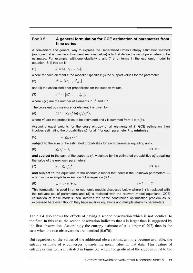
Box 3.5 A general formulation for GCE estimation of parameters from

time series A convenient and general way to express the Generalised Cross Entropy estimation method (and one that is used in subsequent sections below) is to first define the set of parameters to be estimated. For example, with one elasticity σ and 𝑇 error terms in the economic model in equation (3.1) this set is

(1) 𝑆 = {𝜎𝜎, 𝑒𝑒1 , … , 𝑒𝑒𝑇},

where for each element 𝑘 the modeller specifies: (i) the support values for the parameter

(2) 𝑧𝑘 = �𝑧1𝑘, … , 𝑧𝑛(𝑘)𝑘 �

and (ii) the associated prior probabilities for the support values

(3) 𝜋𝜋′𝑘 = �𝜋𝜋1′𝑘, … , 𝜋𝜋𝑛(𝑘)′𝑘 �,

where 𝑛(𝑘) are the number of elements in 𝑧𝑘 and 𝜋𝜋′𝑘.

The cross entropy measure for element 𝑘 is given by

(4) 𝐶𝐸𝑘 = ∑ 𝜋𝜋𝑗𝑘 ln�𝜋𝜋𝑗𝑘 𝜋𝜋𝑗′𝑘� �𝑗 ,

where 𝜋𝜋𝑗𝑘 are the probabilities to be estimated and 𝑗 is summed from 1 to 𝑛(𝑘).

Assuming equal weights for the cross entropy of all elements of 𝑆, GCE estimation then involves estimating the probabilities 𝜋𝜋𝑗𝑘 for all 𝑗 for each parameter 𝑘 to minimise:

(5) 𝐶𝐸 = ∑ 𝐶𝐸𝑘𝑘∈𝑆

subject to the sum of the estimated probabilities for each parameter equalling unity:

(6) ∑ 𝜋𝜋𝑗𝑘 = 1𝑗 , ∀ 𝑘 ∈ 𝑆

and subject to the sum of the supports 𝑧𝑗𝑘, weighted by the estimated probabilities 𝜋𝜋𝑗𝑘 equalling the value of the unknown parameters:

(7) 𝑘 = ∑ 𝜋𝜋𝑗𝑘𝑧𝑗𝑘𝑗 , ∀ 𝑘 ∈ 𝑆

and subject to the equations of the economic model that contain the unknown parameters — which in the example from section 3.1 is equation (3.1),:

(8) 𝑞𝑡 = 𝜎𝜎 ∙ 𝑝𝑡 + 𝑒𝑒𝑡, t = 1, … , 𝑇

This formulation is used in other economic models discussed below where (1) is replaced with the relevant set of parameters and (8) is replaced with the relevant model equations. GCE estimation of these models then involves the same constrained optimisation problem as is expressed here even though they have multiple equations and multiple elasticity parameters.

Table 3.4 also shows the effects of having a second observation which is not identical to the first. In this case, the second observation indicates that σ is larger than is suggested by the first observation. Accordingly the entropy estimate of σ is larger (0.707) than is the case when the two observations are identical (0.670).

But regardless of the values of the additional observations, as more become available, the entropy estimate of σ converges towards the mean value in that data. This feature of entropy estimation is illustrated in Figure 3.1 where the gradient of the slope is equal to the

24 CONFERENCE PAPER

parameter σ being estimated. With each additional observation the estimate of σ is less dependent on the prior and more reflective of its mean value in the data.

Figure 3.1 Stylised effect of additional observations

3.4 Comparing the Ordinary Least Squares and the entropy estimators when data are limited

Monte Carlo methods are used in this section to compare the advantages of the entropy estimator over the Ordinary Least Squares (OLS) estimator when data are limited.

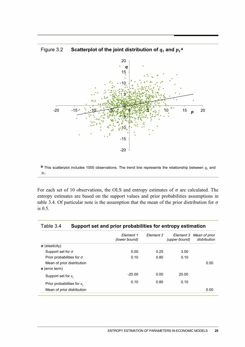
The estimated equation is (3.1) and it is assumed that the true value of 𝜎𝜎 is 0.25 and that 𝑒𝑒𝑡 is normally distributed with a mean of zero and a standard deviation of 5. It is assumed that there are only 10 observations to estimate the elasticity.

To compare the OLS and entropy estimates of 𝜎𝜎 under these assumptions, 10 000 sets of 10 observations are generated. Figure 3.2 provides a scatterplot showing the correlation between 𝑞𝑡 and 𝑝𝑡.

-3

-2

-1

0

1

2

3

-6 -4 -2 0 2 4 6


q

p

-3

-2

-1

0

1

2

3

-6 -4 -2 0 2 4 6

t = 1

q

p

-3

-2

-1

0

1

2

3

-6 -4 -2 0 2 4 6

t = 20

q

p

-3

-2

-1

0

1

2

3

-6 -4 -2 0 2 4 6

t = 100

q

p


Figure 3.2 Scatterplot of the joint distribution of 𝒒𝒕 and 𝒑𝒕 6T

a

a This scatterplot includes 1000 observations. The trend line represents the relationship between 𝑞𝑡 and 𝑝𝑡.

For each set of 10 observations, the OLS and entropy estimates of 𝜎𝜎 are calculated. The entropy estimates are based on the support values and prior probabilities assumptions in table 3.4. Of particular note is the assumption that the mean of the prior distribution for 𝜎𝜎 is 0.5.

Table 3.4 Support set and prior probabilities for entropy estimation


Element 2 Element 3 (upper bound)


σ (elasticity) Support set for σ 0.00 0.25 3.00 Prior probabilities for σ 0.10 0.80 0.10 Mean of prior distribution 0.50

e (error term)

Support set for 𝑒𝑒𝑡 -20.00 0.00 20.00

Prior probabilities for 𝑒𝑒𝑡 0.10 0.80 0.10

Mean of prior distribution 0.00

-20

-15

-10

-5

0

5

10

15

20

-20 -15 -10 -5 0 5 10 15 20

q

p

26 CONFERENCE PAPER

Figure 3.3 presents the distribution of the OLS and entropy estimators of σ. The first point to note is that the mean of the OLS estimator (0.25) is equal to the true value of σ, whereas the mean of the entropy estimator (0.39) is biased in that it deviates from the true value of σ.

Figure 3.3 Distribution of OLS and entropy estimates of σ

Although an unbiased estimator is generally preferable to a biased estimator, in this example the variance of the OLS estimator (0.12) is much larger than the variance of the GCE estimator (0.02). This means that any individual OLS estimate of σ has the potential to deviate quite significantly from the true value of σ.

Indeed, if a modeller relied on the OLS estimator to estimate the value of σ, there is a 23 per cent probability that they would obtain a negative estimate for σ (figure 3.4). In contrast, it is not possible for the entropy estimator to produce an estimate that is less than zero, because the prior distribution is bounded by zero.

Not only does entropy estimation avoid values that are inconsistent with the underlying model, it also is more likely to improve on prior assumptions about the value of parameters in this case (figure 3.4). Suppose that if the modeller did not use an estimate of σ for their economic model, they would assume a value of 0.5 (the prior mean). In this example, there is a 78 per cent chance that the entropy estimate would be an improvement over assuming a value of 0.5 (if an improvement is defined as an estimate that is close to the ‘true’ value

0%

5%

10%

15%

20%

-1.00 -0.75 -0.50 -0.25 0.00 0.25 0.50 0.75 1.00 1.25 1.50

entropy OLS

mean of OLS estimator = 0.25

mean of entropy estimator = 0.39


of 0.25, i.e. between 0.20 and 0.50). In contrast, there is only a 34 per cent chance that the OLS estimate would be located between 0.20 and 0.50.

Figure 3.4 The entropy estimator of σ is preferable in this example

3.5 When is the entropy estimator preferable?

The previous example highlights the tradeoff that exists when choosing between the entropy estimator and an alternative econometric estimator. The benefit of the entropy estimator is that the variance of the estimates tends to be much smaller compared to alternative estimators, but the cost is that the entropy estimator can be biased. For the entropy estimator to be preferable to an alternative estimator, the benefits need to outweigh the costs.

There will be net benefits in choosing the entropy estimator over an alternative estimator if (i) there is useful prior information and (ii) the variance of the alternative estimator is relatively large.

0%

5%

10%

15%

20%

-1.00 -0.75 -0.50 -0.25 0.00 0.25 0.50 0.75 1.00 1.25 1.50

entropy OLS

23% of OLS results < 0

Most entropy results between 0.2 and 0.5

28 CONFERENCE PAPER

There is useful prior information

Useful prior information reduces the variance of the entropy estimator, which in turn increases the chance of obtaining sensible results. It also reduces the bias associated with the entropy estimator.

Two important sets of prior information have a slightly different effect on the entropy estimator.

• The lower and upper bounds of the support values represent absolute restrictions on the entropy estimate; they can significantly reduce the variance of the entropy estimator and force the entropy estimate to produce only results that are within the specified range.

• The prior probabilities can also reduce the variance of the estimator; unlike the lower and upper bounds, the effect of prior probabilities on the entropy estimator diminishes as the number of observations increase.

What if the prior information is ‘wrong’?

Entropy estimation necessarily leads to biased estimates unless the mean of the prior probability distribution is exactly equal to the true value.

• The further the ‘true’ value of an unknown parameter is from the mean of the prior probability distribution, the more biased the entropy estimate.

– If the true value of an unknown parameter is between the lower and upper bound of the support values, then the entropy estimator will still be consistent (as the number of observations increases, the estimator will converge to the ‘true’ value).

– If the true value is not between the lower and upper bound of the support values, then the entropy estimator will be inconsistent (it will always be biased, no matter how many observations are available.7

All else being equal, the more biased the entropy estimator, the more likely it is that an alternative estimator will be preferable. This underscores the need to have credible, well-motivated priors.

What if the prior information is uninformative?

There is little difference between the entropy estimator and alternative estimators if the prior information used is uninformative (the prior probability distribution is close to

7 Practically speaking, obtaining an entropy estimate that is very close to a bound when there are a large

number of observations available, should prompt the modeller to re-examine whether the bounds and prior distribution are appropriate.


uniform over a wide range of values). This is because the entropy estimator is not receiving any assistance from the prior probability distribution.

The variance of the alternative estimator needs to be relatively large

The entropy estimator tends to have a relatively small variance if there is useful prior information. If the variance of an alternative estimator is also relatively small, then the alternative estimator will be preferable as it will be unbiased. However if the variance of the alternative estimator is relatively large, meaning an estimate could differ substantially from the true value of the parameter, the entropy estimator is likely to be preferable.

To see the situations in which the variance of alternative estimators might be large, consider equation 3.6 which is one representation of the formula for the variance of the OLS estimator (Greene 2007, p. 59):

(3.6) 𝑣𝑎𝑟��̂�𝑘� = 𝜎2

�1−𝑅𝑘2�∙∑ (𝑥𝑖𝑘−�̅�𝑘)2𝑛

𝑖

Here:

�̂�𝑘 is the parameter associated with the kth explanatory variable,

𝑥𝑖𝑘 is ith observation of the kth explanatory variable,

𝜎𝜎2 is the variance of the error term, and

𝑅𝑘2 is the coefficient of determination in a regression of 𝑥𝑘, using all other variables as explanatory variables.8

8 The coefficient of determination can be interpreted as the percentage of the variation in variable (𝑥𝑘) that

can be explained by variation in the other explanatory variables.

30 CONFERENCE PAPER

Equation 3.6 suggests that there are four reasons why the variance of an estimated parameter might be large:

• The variance of the error term (𝜎𝜎2) could be large; this could be because of omitted variables or inexact data collection methods.

• There may be few observations (n is small); in most cases, if there are more than a few observations (more than 20), the variance of the alterative estimator is likely to be too small for the entropy estimator to be preferable.

• The variance of the explanatory variable linked to the kth parameter may be relatively small; that is, the values that the kth explanatory variable takes might all be very similar. 9

• There may be a high degree of collinearity between the explanatory variables; that is, the explanatory variables might move together which in equation 3.6 would be characterised by 𝑅𝑘2 being close to one.

In practice, the economic data used for modelling is often limited and noisy and thus the variance of alternative estimators tend to be large. This suggests that if there is useful prior information about parameter values, the net benefits of using entropy estimation will likely be large.

3.6 How to make assumptions about support values and prior probabilities

Theoretically, it should be easy to choose the ‘right’ probability distribution — as noted in box 3.1, the modeller should choose a distribution that reflects the uncertainty surrounding the values that the unknown parameters can take. However, modellers may not be confident about (or may not agree on) the underlying distribution. For this reason, it is important to consider how assumptions about support values and prior probability distributions affect the properties of entropy estimation.

Bounds on support values

As noted above, the smaller the range of the bounds on the support values, the more likely it is that the true value of the parameter is not within those bounds (and the entropy estimate is inconsistent). But if the true value is within those bounds, then the estimator will be consistent and the variance of the estimator will small. Thus the choice of bounds will be determined by a tradeoff between efficiency and consistency.

9 The estimated variance of the independent variable is calculated as:

1𝑛

× ∑ (𝑥𝑖𝑘 − �̅�𝑘)2𝑛𝑖 .


Additionally, it is important to note that the bounds of the support values for the error term should be sufficiently large so that they are never binding. If the estimate of the error term is equal to one of its bounds, the parameter estimate will be biased to accommodate the misspecified error term.

Number of elements in the support values

For a given set of bounds on the support values, the choice of the number of elements in the support values has two competing effects.

• The more elements there are, the easier it is to represent prior information about the unknown parameter. For example, it is easier to represent a normal-like distribution when there are five elements in the support values, than when there are three elements. With only three elements in the support values, it is hard to represent all but the simplest of distributions if there are theoretical bounds which should only be associated with a very small amount of prior probability.

• The problem becomes more difficult computationally as the number of elements in the support values increases. This is because increasing the support values adds variables to the objective function and increases the size of the optimisation problem to solve. Indeed, if an element is added to the support values for the error term, then a variable is added to the objective function for each observation.

In most cases, setting the support values to include five elements seems like an appropriate starting point. This allows for normal-like prior distributions while not making the problem too difficult to solve.

Prior probabilities

As noted above, the prior probabilities (in conjunction with the support values) will bias the entropy estimate unless the mean of the prior distribution is equal to the true value of the parameter. That said, unlike the choice of bounds, the influence of the prior probabilities diminishes as the number of observations increases. Thus for a large set of observations, the priors chosen will have little effect on the entropy estimate.

32 CONFERENCE PAPER

4 Using cross entropy to estimate elasticities from time series: Part II multiple equations

The complicating factor that often arises when estimating multi-equation models is the presence of simultaneous-equation bias.10 This occurs when two or more endogenous variables are determined by the system (the equations are not independent) and the estimation technique used does not account for this interdependency. The bias arises because the assumption that the regressors are uncorrelated with the residual does not hold.

A simple example of simultaneous equations that cannot be estimated consistently using OLS or entropy is the percentage change supply and demand equations:

(4.1) 𝑞𝑑,𝑡 = 𝛼1𝑝𝑡 + 𝛼2𝑦𝑡 + 𝑒𝑒𝑑,𝑡 t = 1, ... , T

(4.2) 𝑞𝑠,𝑡 = 𝛽1𝑝𝑡 + 𝛽2𝑥𝑡 + 𝑒𝑒𝑠,𝑡 t = 1, ... , T

(4.3) 𝑞𝑑,𝑡 = 𝑞𝑠,𝑡 = 𝑞𝑡 t = 1, ... , T

where the 𝛼 and 𝛽 are elasticities, 𝑞𝑠,𝑡 and 𝑞𝑑,𝑡 are percentage changes in the quantity demanded and supplied of a good, 𝑝𝑡 is the percentage change in the price, 𝑦𝑡 is the percentage change in income and 𝑥𝑡 is the percentage change in unit costs. Both 𝑦𝑡 and 𝑥𝑡 are exogenous, and 𝑝𝑡 and 𝑞𝑡 are endogenous.

There are two main approaches to countering simultaneity bias in entropy estimation:11

• using a structural equation entropy estimator (analogous to two-stage least squares estimation), discussed in section 4.1;

• allowing endogenous variables to be determined endogenously in the estimation process (‘endogenous variables entropy estimator’), discussed in section 4.2.

Sections 4.3 uses Monte Carlo simulations to compare the structural equation entropy estimator, endogenous variables entropy estimator, and the simple entropy estimator of the elasticities in equations 4.1 through 4.3.

4.1 A structural equation entropy estimator

In traditional econometric techniques, simultaneous equation bias is typically avoided by using instrumental variables in a two-stage or three-stage least squares estimation procedure (Greene 2007). These estimators avoid simultaneity bias by:

10 Harmon, Preckel and Eales (1998) develop a entropy estimator to estimate linear systems of equations

where the errors are correlated across equations, but where there is no simultaneous equation bias. 11 Both these approaches can also be used to address simultaneous-equation bias in nonlinear models. For

example, Arndt, Robinson and Tarp (2001) use the endogenous variables approach to estimate parameter values for nonlinear multi-equation models.


• estimating the relationship between the endogenous regressor and all the exogenous regressors;

• using this relationship to calculate predicted values for the endogenous regressor; and

• using these predicted values in place of the original values for the endogenous right-hand-side variables in an OLS estimation of each model equation.12

In the above supply-demand example, the two-stage least squares estimator would involve first estimating:

(4.4) 𝑝𝑡 = 𝛿1𝑦𝑡 + 𝛿2𝑥𝑡 + 𝑒𝑒𝑝,𝑡 t = 1, ... , T

and then using 4.4 to obtain the predicted values �̂�𝑡:

(4.5) �̂�𝑡 = 𝛿1𝑦𝑡 + 𝛿2𝑥𝑡 t = 1, ... , T

which are then used to estimate equations 4.6 and 4.7 using OLS:

(4.6) 𝑞𝑡 = 𝛼1�̂�𝑡 + 𝛼2𝑦𝑡 + 𝑒𝑒𝑑,𝑡 t = 1, ... , T

(4.7) 𝑞𝑡 = 𝛽1�̂�𝑡 + 𝛽2𝑥𝑡 + 𝑒𝑒𝑠,𝑡 t = 1, ... , T

A similar approach can be applied to entropy estimation. Marsh, Mittelhammer and Cardell (1998) developed a structural-equation entropy estimator that avoids simultaneous equation bias. Like two-stage least squares, this estimator uses exogenous regressors to obtain predicted values for the endogenous regressors. These imputed values are used in place of the actual values to estimate the model equations. Unlike two-stage least squares, the Marsh, Mittelhammer and Cardell formulation estimates both types of equations simultaneously.13

A convenient way to express the entropy estimation equations for this estimator is to use the GCE formulation set out above in box 3.5.

First define the set of parameters to be estimated. In the Marsh, Mittelhammer and Cardell estimator for equations 4.4 through 4.7, this set is:

(4.8) S = �𝛼1,𝛼2, β1,β2, 𝛿1,𝛿2,𝑒𝑒𝑝,1, 𝑒𝑒𝑑,1, 𝑒𝑒𝑠,1, … , 𝑒𝑒𝑝,𝑇 , 𝑒𝑒𝑑,𝑇 , 𝑒𝑒𝑠,𝑇�

which replaces the set in equation 1 in box 3.5. For each element k it is necessary to specify the support values of possible parameter values and associated prior probabilities (2 and 3 in box 3.5).

12 If there are multiple endogenous regressors, this process can be expanded, with a separate relationship

estimated (using exogenous regressors) for each endogenous regressor to obtain predicted values. 13 It is also possible to solve two separate entropy estimation problems — one to obtain predicted values for

the endogenous regressors and one to estimate the unknown parameters. This estimator produces broadly similar results to the structural equation estimator.

34 CONFERENCE PAPER

Then Generalised Cross Entropy estimation involves minimising the aggregate cross entropy measure (5 in box 3.5) subject to:

• the sum of the estimated probabilities for each parameter equalling unity (6 in box 3.5)

• the sum of the supports weighted by the estimated probabilities equalling the value of the unknown parameters (7 in box 3.5)

• the 4T equations of the model in equations 4.4 through 4.7 (which replace the equations in 8 in box 3.5).


4.2 Endogenous variables approach

The approach used by Arndt, Robinson and Tarp (2001), Liu, Arndt and Hertel (2000) and Go et al. (2014) to avoid simultaneous equation bias allows the entropy estimation model to determine the variables that are considered endogenous in the economic model (such as prices and quantities in the previous example). The error terms are the differences between the calculated values for these variables and their historically observed values. Thus the error terms are associated with the endogenous variables, not the equations as is the case with the structural equation approach.

Returning to the supply-demand example in equations 4.1 through 4.3, the estimating model can be re-specified as:

(4.9) 𝑞�𝑡 = 𝛼1�̂�𝑡 + 𝛼2𝑦𝑡 t = 1, ... , T

(4.10) 𝑞�𝑡 = 𝛽1�̂�𝑡 + 𝛽2𝑥𝑡 t = 1, ... , T

(4.11) 𝑞𝑡 = 𝑞�𝑡 + 𝑒𝑒1,𝑡 t = 1, ... , T

(4.12) 𝑝𝑡 = �̂�𝑡 + 𝑒𝑒2,𝑡 t = 1, ... , T

With this specification, �̂�𝑡 and 𝑞�𝑡 are the values of the endogenous variables that are calculated in the entropy estimation and 𝑝𝑡 and 𝑞𝑡 are the actual observed values.

An important way to view these 4T equations is that they contain 4T endogenous variables (�̂�𝑡, 𝑞�𝑡, 𝑒𝑒1,𝑡, 𝑒𝑒2,𝑡) and 4T exogenous variables that take on their historical values (𝑦𝑡, 𝑥𝑡 , 𝑝𝑡, 𝑞𝑡).

One use of these equations would be in a historical validation of a model (Dixon and Rimmer 2013) where the initial priors for the elasticities are used to solve the model in each period. Examination of the errors then gives an indication of how well the model tracks historically.

The endogenous variables approach for GCE estimation can be seen as a generalisation of this model validation. It goes further by adjusting the prior estimates of the elasticities to better fit the historical data, and thus it will improve the tracking performance of the economic model. As noted in section 3.3, the more historical observations available, the more the elasticity estimates will reflect what is in the data and not the priors.

A particular strength of the endogenous-variables approach is that it is easier to implement than the structural-equation estimator, especially for large models. Adding the error equations to the endogenous variables in an economic model is much simpler than adding numerous structural equations. In addition, the error values themselves are of considerable interest in model evaluation.

36 CONFERENCE PAPER

With the endogenous variables approach for entropy estimation, the set of parameters to be estimated is:

(4.13) S = �𝛼1,𝛼2, β1,β2, 𝑒𝑒1,1, 𝑒𝑒2,1, … , 𝑒𝑒1,𝑇 , 𝑒𝑒2,𝑇�

which replaces the set of parameters in 1 in the general formulation for GCE estimation in box 3.5. Again, the support values and associated probabilities (2 and 3 in box 3.5) need to be specified for each parameter.

The endogenous variable entropy estimator then involves minimising the aggregate cross entropy measure (5 in box 3.5), subject to estimated probabilities for each parameter equalling unity (6 in box 3.5), subject to the sum of the supports weighted by the estimated probabilities equalling the value of the unknown parameter (7 in box 3.5) and subject to the 4T equations in 4.9 through 4.12.

An issue to be aware of with the endogenous variables approach is whether the model is identified; if it is not then it will not provide consistent estimates. This can happen if, for a given set of exogenous variables, more than one set of parameters generates the same set of observations for the outcome variables.14 The model in equations 4.9 through 4.12 is identified because there is only one feasible combination of the parameters for given values of 𝑞𝑡, 𝑝𝑡, 𝑦𝑡, 𝑥𝑡, 𝑒𝑒1,𝑡 and 𝑒𝑒2,𝑡. Thus the entropy estimators for 𝛼1, 𝛼2, 𝛽1 and 𝛽2 will be consistent. This is illustrated in the Monte Carlo results below in section 4.3 as well as an example of inconsistent estimators from an unidentified model (a model with equations 4.9 through 4.11 only).

14 The problem of identification can also apply to the structural-equation entropy estimator. If the structural

equation entropy estimator is not identified, the endogenous variables entropy estimator is necessarily not identified. That said, unless there is an outcome equation for every endogenously determined variable, the endogenous variables approach is at a greater risk of identification problems.


4.3 Some Monte-Carlo simulations — consistency of the estimators and effectiveness with small samples

In this section two sets of Monte Carlo simulations are undertaken to:

• assess the consistency of the estimators (whether the estimators converge to the true value as the number of observations increase) (section 4.3.1)

• compare the effectiveness of the structural equation and endogenous variables entropy estimators at estimating a model with 10 observations (section 4.3.2).

Table 4.1 presents the specifications for the two sets of Monte Carlo simulations.

Table 4.2 presents the support values and prior distributions used for the unknown parameters in equations 4.1 through 4.3.

Table 4.1 Monte Carlo simulation specifications

Base Case

Distribution of 𝑦𝑡and 𝑧𝑡 Normal(0,1) Distribution of 𝑒𝑒𝑑,𝑡 and𝑒𝑒𝑠,𝑡 Normal(0,1) True value of α1 -2 True value of α2 2 True value of 𝛽1 0.5 True value of 𝛽2 -2

Consistency simulations (section 4.3.1) Number of observations 1 000 Number of simulations 100

38 CONFERENCE PAPER

Table 4.2 Support set and prior probabilities for entropy estimation




𝜶𝟏 Support set -6.00 -1.00 0.00 Prior probabilities 0.10 0.80 0.10 -1.40

𝜶𝟐 Support set 0.00 1.00 6.00 Prior probabilities 0.10 0.80 0.10 1.40

𝜷𝟏 Support set 0.00 0.50 3.00 Prior probabilities 0.10 0.80 0.10 0.70

𝜷𝟐 Support set for -6.00 -1.00 0.00 Prior probabilities 0.10 0.80 0.10 -1.40

𝒆𝒅,𝒕 and 𝒆𝒔,𝒕 Support set -4.00 0.00 4.00 Prior probabilities 0.10 0.80 0.10 0.00

4.3.1 Consistency of the estimators

The simple entropy estimator is not consistent

Table 4.3 presents the results from estimating the simultaneous equation supply-demand model in equations 4.1 through 4.3 with a large number of observations. The assumed supports and probabilities are from table 4.2.

As can be seen in table 4.3, the absolute difference between the estimates and the true values is between 0.32 and 0.42 for all parameters. This suggests that the estimator is not consistent as the average of 100 simulations of 1000 observations would be much closer to zero if it were consistent.

Table 4.3 Simple entropy elasticity estimates

Average estimatea True value Difference

𝛼1 -1.58 -2.00 0.42 α2 1.66 2.00 -0.34 𝛽1 0.11 0.50 -0.39 𝛽2 -1.68 -2.00 0.32

a Based on the average of 100 simulations of 1000 observations.


The structural equation entropy estimator is consistent

The elasticity estimates based on the structural equation entropy estimator for the model in equations 4.4 through 4.8 are presented in table 4.4. Table 4.5 documents the assumed supports and probabilities additional to those in table 4.2.

Table 4.4 illustrates that the structural equation entropy estimator provides average elasticity estimates that are almost identical to the true values when there are a large number of observations available.

Table 4.4 Structural equation elasticity estimates


𝛼1 -2.00 -2.00 0.00 α2 1.99 2.00 -0.01 𝛽1 0.51 0.50 0.01 𝛽2 -2.00 -2.00 0.00 𝛿1 0.80 0.80 0.00 𝛿2 0.80 0.80 0.00


Table 4.5 Support set and prior probabilities for structural equation

entropy estimation (additional to table 4.2)




𝜹𝟏 Support set 0.00 0.50 2.67 Prior probabilities 0.10 0.80 0.10 0.67

𝜹𝟐 Support set 0.00 0.50 2.67 Prior probabilities 0.10 0.80 0.10 0.67

𝒆𝒑,𝒕

Support set -4.00 0.00 4.00 Prior probabilities 0.10 0.80 0.10 0.00

The endogenous variables entropy estimator is consistent

The elasticity estimates based on the endogenous variables entropy estimator for the model in equations 4.9 through 4.11 are presented in table 4.6. The assumed supports and probabilities additional to those in table 4.2 are provided in table 4.7.

40 CONFERENCE PAPER

As is clear in table 4.6 the endogenous variables entropy estimator also provides consistent estimates.

Table 4.6 Endogenous-variables elasticity estimates


𝛼1 -1.99 -2.00 0.01 α2 1.99 2.00 -0.01 𝛽1 0.51 0.50 0.01 𝛽2 -2.00 -2.00 -0.00


Table 4.7 Support set and prior probabilities for endogenous variables

entropy estimation (additional to table 4.2)




𝒆𝟏,𝒕 and 𝒆𝟐,𝒕 Support set -4.00 0.00 4.00 Prior probabilities 0.10 0.80 0.10 0.00

The endogenous-variables entropy estimator is inconsistent if it is underidentified

As briefly noted in section 4.2, for the endogenous-variables entropy estimator to be consistent, the model must be identifiable. Equations 4.9 through 4.10 on their own, (ie not including equation 4.11) represent an endogenous variables specification of the linear demand-supply model that is not identifiable.

Table 4.8 presents the elasticity values that result from applying the endogenous variables estimator to this unidentified system. As can be seen from the differences between the estimates and the true values, the estimator is not consistent.

This example also illustrates that an important way to achieve identification in an unidentified model is to include more outcome variables (i.e. include equation 4.11), but this approach can only be used if data are available for the additional variables.


Table 4.8 Underidentified endogenous-variables elasticity estimates


𝛼1 -1.60 -2.00 0.40 α2 1.46 2.00 -0.54 𝛽1 0.61 0.50 0.11 𝛽2 -2.21 -2.00 -0.21


4.3.2 Comparing the effectiveness of the estimators with small samples

10 000 Monte Carlo simulations of 10 observations were generated. For each simulation, a structural-equation entropy estimate and a (consistent) endogenous-variables entropy estimate were calculated. Figure 4.1 plots the distributions of the results for the two estimators.

As can be seen the distributions of structural-equation entropy estimates and the endogenous-variables entropy estimates are similar. Both estimators produce almost the same distribution of estimates for 𝛽1 and 𝛽2. The structural-equation entropy estimator is less biased for all parameters, but the difference is only substantial for 𝛼1 as can be seen in table 4.9.

42 CONFERENCE PAPER

Figure 4.1 Monte Carlo simulation results for the structural equation

and endogenous variables entropy estimatorsa

Structural-equation estimates Endogenous variables estimates

a Based on 1 000 simulations of 10 observations.

Table 4.9 Comparing the mean estimates of the structural-equation

and endogenous-variables entropy estimatesa

Mean of structural-equation parameter estimates

Mean of endogenous-variables parameter estimates

True value

𝛼1 -1.65 -1.81 -2.00 α2 1.64 1.66 2.00 𝛽1 0.61 0.63 0.50 𝛽2 -1.97 -2.01 -2.00


0%5%

10%15%20%25%30%35%

-4.00 -3.00 -2.00 -1.00 0.000%

5%

10%

15%

20%

25%

30%

35%

0.00 1.00 2.00 3.00 4.00

0%5%

10%15%20%25%30%35%

0.00 1.00 2.00 3.00 4.000%5%

10%15%20%25%30%35%

-4.00 -3.00 -2.00 -1.00 0.00


5 Concluding remarks

Traditional econometric techniques are effective at estimating parameters when a large number of observations are available. This is because as the number of observations increase, the variance of traditional estimators shrink (we are more confident about the estimate) (Greene 2007). When only a few observations are available, the variance of traditional estimators can be quite large, even infinite for underdetermined models. In these circumstances, an estimate may deviate significantly from the true value. Indeed using traditional estimators when the data is limited may even produce estimates that that are inconsistent with well-tested economic theory.

Modellers tend to avoid these problems by not estimating relationships when the data are limited and noisy. But when a model requires a value for a particular parameter, modellers are forced to either choose values based on judgment or use econometric estimates that have large standard errors.

Entropy estimation is a useful technique for estimating relationships in these circumstances. It enables economic modellers to improve the assumptions they make about parameter values in economic models when the available data are limited and the variance of alternative estimators are large. With limited data, parameter estimates depend on the priors, but as new data becomes available the estimates depend more on the data.

An important feature of entropy estimation is that the parameter estimates are obtained as part of solving the economic model itself. That is, the estimating equations are those in the model and indeed the parameter estimates must satisfy the constraints of all model equations in all periods. The alternative and more common practice is that the equations used to estimate parameters are separate from the economic model and the econometrics is done outside of the model. In such cases the resulting parameter estimates, which are subsequently used in solving the economic model, may come from estimating equations that are quite different from those in the model.

Of particular interest for simultaneous equation CGE modelling is the endogenous variables entropy estimator. With this approach, additional equations for errors are added to the CGE model specifying the difference between the calculated values for endogenous variables and their actual observed values for each period in which data are available. Thus for each period if there are m observable endogenous variables then m equations are added to the CGE model along with m endogenous error terms. If the assumed priors for elasticity values were used to solve the model in each period, examination of the errors – the difference between calculated and actual values – would provide a goodness-of-fit validation test of the model, and it would be a starting point for entropy estimation to improve those elasticity values. With ever-increasing computing power and usable time series data available, that exercise is now becoming possible.

44 CONFERENCE PAPER

References Arndt, C., Robinson, S. and Tarp, F. 2001, Parameter estimation for a computable general

equilibrium model: a maximum entropy approach, TMD discussion paper, 40, International Food Policy Research Institute, Washington, D.C., pp. 375–398.

Dixon, P.B. and Jorgenson, D. 2012, Handbook of Computable General Equilibrium Modeling, Newnes.

—— and Rimmer, M.T. 1998, Forecasting and Policy Analysis with a Dynamic CGE Model of Australia, Monash University, Centre of Policy Studies/IMPACT Centre.

Dixon, P.B. and Rimmer, M.T. 2013, Validation in Computable General Equilibrium Modeling, Handbook of Computable General Equilibrium Modeling, Elsevier, pp. 1271–1330, http://econpapers.repec.org/bookchap/eeehacchp/v_3a1_3ay_3a2013_3ai_3ac_3ap_3a1271-1330.htm (accessed 21 January 2015).

Go, D.S., Lofgren, H., Ramos, F.M. and Robinson, S. 2014, ‘Estimating Parameters and Structural Change in CGE Models Using a Bayesian Cross-Entropy Estimation Approach’, https://www.gtap.agecon.purdue.edu/resources/download/6960.pdf (accessed 21 January 2015).

Golan, A., Judge, G. and Miller, D. 1996, Maximum entropy econometrics: Robust estimation with limited data, John Wiley.

Greene, W.H. 2007, Econometric Analysis, 6th edn, Prentice Hall.

Harmon, A., Preckel, P.V. and Eales, J. 1998, Entropy-Based Seemingly Unrelated Regression, Department of Agricultural Economics, Purdue University, http://ageconsearch.umn.edu/bitstream/28682/1/sp98-08.pdf (accessed 23 April 2014).

Howitt, R. and Reynaud, A. 2003, ‘Spatial disaggregation of agricultural production data using maximum entropy’, European Review of Agricultural Economics, vol. 30, no. 3, pp. 359–387.

Howitt, R.E. 2005, ‘Agricultural and environmental policy models: Calibration, estimation and optimization’, Davis: University of California, Davis. Available online at< http://www. agecon. ucdavis. edu/people/faculty/facultydocs/howitt/master. pdf.

—— and Msangi, S. 2006, ‘Estimating disaggregate production functions: An application to Northern Mexico’, presented at the Annual Meeting of the American Agricultural Economics Association, http://www.infoandina.org/sites/default/files/publication/files/AAEAPaper_HowittMsangi_July21st2006_.pdf (accessed 21 January 2015).

Jaynes, E.T. 1963, ‘Information Theory and Statistical Mechanics (Notes by the lecturer)’, vol 1, presented at the Statistical Physics 3, pp. 181–218, http://adsabs.harvard.edu/abs/1963stph.conf..181J (accessed 21 January 2015).


Liu, J., Arndt, C. and Hertel, T. 2000, ‘Estimating trade elasticities for GTAP: A maximum entropy approach’, presented at Third Annual Conference in Global Economic Analysis, Melbourne, Center for Global Trade Analysis, Purdue University.

Marsh, T.L., Mittelhammer, R.C. and Cardell, N.S. 1998, ‘A Structural-Equation GME Estimator’, presented at AAEA Annual Meeting, Salt Lake City.

Paris, Q. and Howitt, R.E. 1998, ‘An Analysis of Ill-Posed Production Problems Using Maximum Entropy’, American Journal of Agricultural Economics, vol. 80, no. 1, pp. 124–138.

Preckel, P.V. 2001, ‘Least Squares and Entropy: A Penalty Function Perspective’, American Journal of Agricultural Economics, vol. 83, no. 2, pp. 366–377.

Robinson, S., Cattaneo, A. and El-Said, M. 2001, ‘Updating and estimating a social accounting matrix using cross entropy methods’, Economic Systems Research, vol. 13, no. 1, pp. 47–64.

Shannon, C.E. 1948, ‘A Mathematical Theory of Communication’, The Bell System Technical Journal, vol. 27, pp. 379–423, 623–656.

Zhang, X. and Verikios, G. 2006, Armington Parameter Estimation for a Computable General Equilibrium Model: A Database Consistent Approach, Economics Discussion / Working Paper, 06-10, The University of Western Australia, Department of Economics.

46 CONFERENCE PAPER

Appendix

The GAMS code below calculates the endogenous variables entropy estimates for the simultaneous equation model in equations 4.9 through 4.12.

It is based on the general GCE formulation set out in box 3.5 and thus can be easily modified to generate the entropy estimates for the other examples in this paper. Notice however that in box 3.5 no distinction is made between elasticity and error parameters whereas in the code below it is convenient to distinguish between the two types of entropy parameters.

Documents

An introduction to entropy estimation of parameters in