Embed Size (px)
Citation preview
Studying material for
Statistical Learning Theory1
Spring Semesters 2013 – 2019
Version 2.0.2of March 14, 2019
Joachim M. Buhmann2
ETH Zürich, D-INFK
1https://ml2.inf.ethz.ch/courses/slt/2This scriptum is based on draft lecture notes typed by Sergio Solórzano, Francesco Locatello
and David Tedaldi. Final merging and editing by Alexey Gronskiy. Formatting based on LATEXtemplate provided by Tobias Pröger.

Contents
1 Notation 7
2 Maximum entropy inference 92.1 General maximum entropy description . . . . . . . . . . . . . . . . . 92.2 Entropy as expected surprise . . . . . . . . . . . . . . . . . . . . . . 92.3 Maximum entropy principle . . . . . . . . . . . . . . . . . . . . . . . 112.4 Most stable inference . . . . . . . . . . . . . . . . . . . . . . . . . . . 12
2.4.1 Minimal sensitivity condition . . . . . . . . . . . . . . . . . . 122.4.2 Least sensitive distribution derivation . . . . . . . . . . . . . 13
2.5 Some examples of least sensitive distributions . . . . . . . . . . . . . 152.6 Maximum entropy inference for k-means clustering . . . . . . . . . . 16
2.6.1 k-means clustering . . . . . . . . . . . . . . . . . . . . . . . . 162.6.2 Maximum entropy clustering . . . . . . . . . . . . . . . . . . 17
2.7 Clustering distributional data . . . . . . . . . . . . . . . . . . . . . . 192.7.1 Distributional data . . . . . . . . . . . . . . . . . . . . . . . . 192.7.2 Histogram clustering cost function . . . . . . . . . . . . . . . 212.7.3 Analogy between k-means and histogram clustering . . . . . 222.7.4 Limitations of histogram clustering . . . . . . . . . . . . . . . 232.7.5 Parametric distributional clustering . . . . . . . . . . . . . . 232.7.6 Parametric distributional clustering . . . . . . . . . . . . . . 24
2.8 Information Bottleneck . . . . . . . . . . . . . . . . . . . . . . . . . . 252.9 Sampling . . . . . . . . . . . . . . . . . . . . . . . . . . . . . . . . . 25
2.9.1 Metropolis Sampling . . . . . . . . . . . . . . . . . . . . . . . 262.9.2 LTS: Gibbs Sampling . . . . . . . . . . . . . . . . . . . . . . 262.9.3 Rejection Sampling . . . . . . . . . . . . . . . . . . . . . . . . 262.9.4 Importance sampling . . . . . . . . . . . . . . . . . . . . . . . 272.9.5 Compute probabilistic centroids and soft assignment . . . . . 27
3 Graph based clustering 293.1 Correlation Clustering . . . . . . . . . . . . . . . . . . . . . . . . . . 303.2 Pairwise data clustering . . . . . . . . . . . . . . . . . . . . . . . . . 313.3 Pairwise clustering as k-means clustering in kernel space . . . . . . . 31
4 Mean field approximation 35
5 Approximation set coding 415.1 Setting and Generative Model Assumptions . . . . . . . . . . . . . . 41
5.1.1 Optimization Problem . . . . . . . . . . . . . . . . . . . . . . 415.1.2 Data Generation Model . . . . . . . . . . . . . . . . . . . . . 42
5.2 Approximation Set-Based Approach . . . . . . . . . . . . . . . . . . 425.2.1 Approximation Sets . . . . . . . . . . . . . . . . . . . . . . . 425.2.2 Communication and Learning Stability . . . . . . . . . . . . . 44
6 Probably Approximately Correct Learning 53
7 Final note 59
A Notions of probability 61
Preface
3 The information age with its digital revolution in engineering, natural sciences, so-cial sciences, economics and humanties confronts us with an unprecedented wealthof data that has to be converted into knowledge. Learning and Information aretwo notions of modern science that capture our ability to model reality by empiricalinference. Learning characterizes the process to acquire knowledge about reality.Information quantifies this knowledge relative to hypothesis classes. The scientificmethod as the process of inference relies on learning predictive models from ob-servations that are commonly collected as data by experimentation. Informationquantitatively assess how precisely these observations discriminate hypotheses thatare algorithmically inferred from data.
The lecture Statistical Learning Theory investigates learning as the knowl-edge acquisition process and information as the knowledge quantification measure.Entropy plays an essential role in both respects and it allows us to establish in-tellectual connections between combinatorics, algorithmics, information theory andclassical Bayesian learning.
3DisclaimerThis script is the first version (2.0.2) of the lecture notes for the course “Statistical Learning Theory”imparted by Prof.Dr Joachim M. Buhmann at ETH Zurich. Shall the reader find any kind ofmistakes, typos, unclear passages or notation please address an e-mail to [email protected] sothe lecture notes can be corrected and improved.

6
Chapter 1
Notation
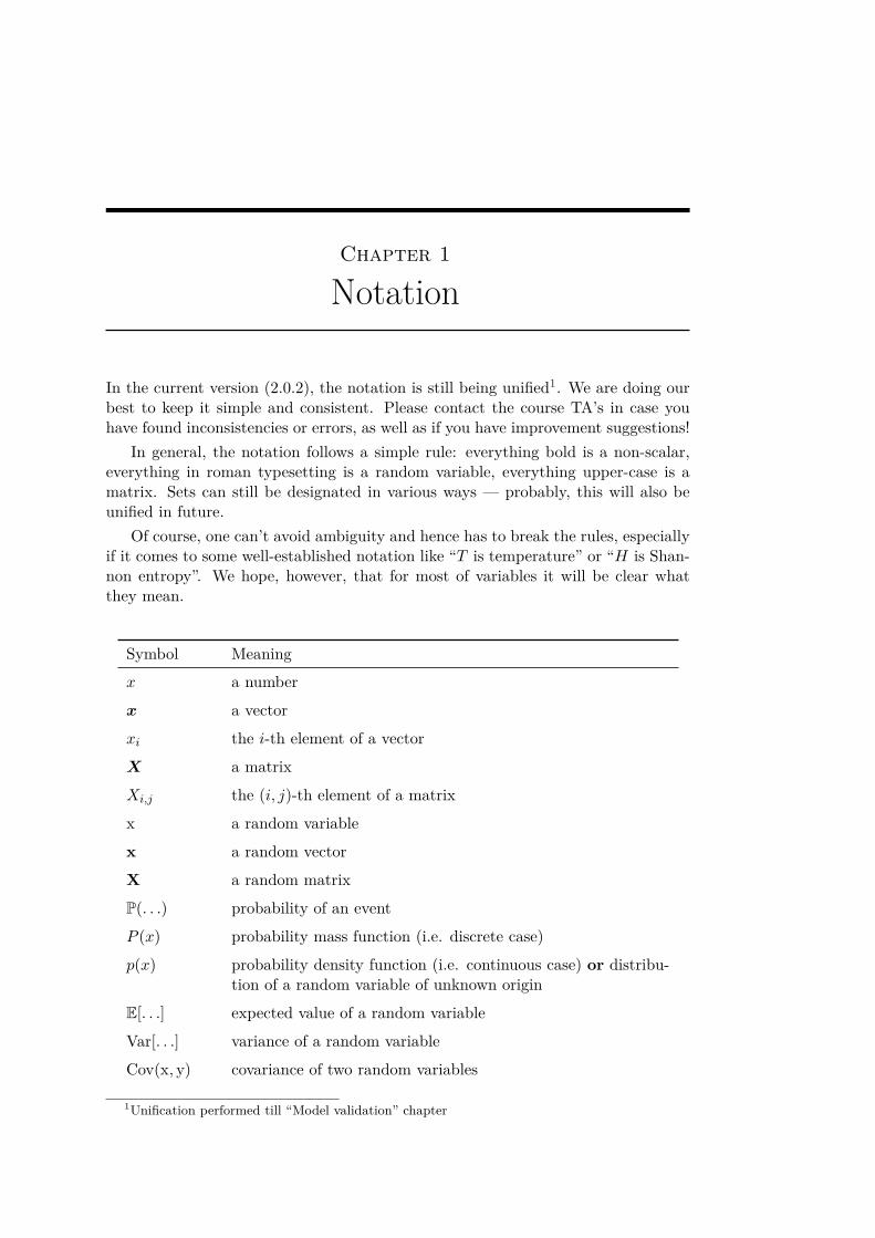
In the current version (2.0.2), the notation is still being unified1. We are doing ourbest to keep it simple and consistent. Please contact the course TA’s in case youhave found inconsistencies or errors, as well as if you have improvement suggestions!
In general, the notation follows a simple rule: everything bold is a non-scalar,everything in roman typesetting is a random variable, everything upper-case is amatrix. Sets can still be designated in various ways — probably, this will also beunified in future.
Of course, one can’t avoid ambiguity and hence has to break the rules, especiallyif it comes to some well-established notation like “T is temperature” or “H is Shan-non entropy”. We hope, however, that for most of variables it will be clear whatthey mean.
Symbol Meaning
x a number
x a vector
xi the i-th element of a vector
X a matrix
Xi,j the (i, j)-th element of a matrix
x a random variable
x a random vector
X a random matrix
P(. . .) probability of an event
P (x) probability mass function (i.e. discrete case)
p(x) probability density function (i.e. continuous case) or distribu-tion of a random variable of unknown origin
E[. . .] expected value of a random variable
Var[. . .] variance of a random variable
Cov(x, y) covariance of two random variables
1Unification performed till “Model validation” chapter
8 Notation
Symbol Meaning
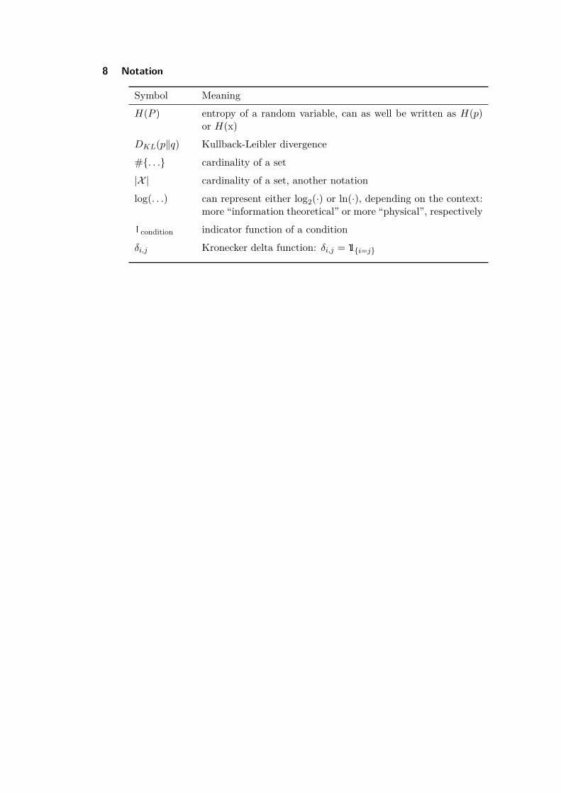
H(P ) entropy of a random variable, can as well be written as H(p)or H(x)
DKL(p‖q) Kullback-Leibler divergence
#. . . cardinality of a set
|X | cardinality of a set, another notation
log(. . .) can represent either log2(·) or ln(·), depending on the context:more “information theoretical” or more “physical”, respectively
1condition indicator function of a condition
δi,j Kronecker delta function: δi,j = 1i=j
Chapter 2
Maximum entropy inference
2.1 General maximum entropy descriptionStatistical inference derives a probabilistic law from particular random instances,e.g., we observe random vectors and we infer the location parameter of the prob-ability density function. In fields such as machine learning, applied mathematics,statistical physics, etc., probability distributions of random variables are often in-fered by matching a fixed number of constraints that are given as expectation valuesof different observables. The constraints most often do not uniquely determine thedisctribution and we therefore can qpose the question: Which distribution thatmatch the constraints is most generic, meaning that it requires the least additionalassumptions?
We will first discuss the case of discrete random variables. Let Ω be a set of mu-tually independent outcomes ωi, the problem is then to determine the probabilitiespi = P(ωi) i = 1, 2, . . . , n given the constraints (“moments”)
µj = E[rj ] =n∑i=1
rj(ωi)pi, (2.1)
where rj : Ω → R j = 1, 2, . . . ,m are different functions defined over Ω. It is clearthat there are m + 1 constraints on the pi thus if m + 1 < n there are not enoughconstraints to unambiguously define the probability distribution. For continuous dis-tributions, it is also the case that a finite number of mean values are not enough tocompletely determine it. An answer to this problem was given by E.T.Jayne and isknown as the “maximum entropy principle” according to which P = p1, p2, . . . , pnmust be such that it respect the constraints but otherwise it is as unbiased (non-committal) as possible. The task of finding P is then achieved by maximizing the“entropy” subject to the given constraints.
In this chapter the idea of entropy will first be introduced as expected valueof surprise in Section 2.2 and then using Jayne’s principle it will be shown thatthe desired distribution has the Gibbs form (Section 2.3). Afterwards the sameresult will be derived (Section 2.4), following the work of ?, by demanding thatthe distribution P is the least sensitive to errors in the values of the µj . Then inSection 2.6 maximun entropy inference is applied to the clustering problem.
2.2 Entropy as expected surpriseLets define a function S that can measure how informative the events A ∈ A of aprobability model (Ω,A,P) are according to the following axioms:
10 Maximum entropy inference
Definition 1 (Surprise).Information as“surprise”
Let (Ω,A,P) be a probability model. The suprise of anevent A is given by S(P(A)), where the function S : [0, 1]→ [0,∞) is characterizedby
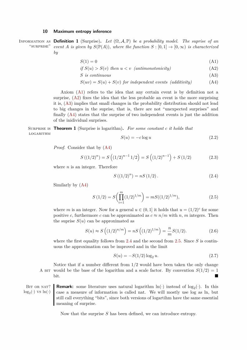
S(1) = 0 (A1)if S(u) > S(v) then u < v (antimonotonicity) (A2)S is continuous (A3)S(uv) = S(u) + S(v) for independent events (additivity) (A4)
Axiom (A1) refers to the idea that any certain event is by definition not asurprise, (A2) fixes the idea that the less probable an event is the more surprisingit is, (A3) implies that small changes in the probability distribution should not leadto big changes in the suprise, that is, there are not “unexpected surprises” andfinally (A4) states that the surprise of two independent events is just the additionof the inidividual surprises.
Theorem 1 (Surprise is logarithm).Surprise islogarithm
For some constant c it holds that
S(u) = −c log u (2.2)
Proof. Consider that by (A4)
S ((1/2)n) = S((1/2)n−1 1/2
)= S
((1/2)n−1
)+ S (1/2) (2.3)
where n is an integer. Therefore
S ((1/2)n) = nS (1/2) . (2.4)
Similarly by (A4)
S (1/2) = S
( m∏i=1
(1/2)1/m)
= mS((1/2)1/m), (2.5)
where m is an integer. Now for a general u ∈ (0, 1] it holds that u = (1/2)c for somepositive c, furthermore c can be approximated as c ≈ n/m with n, m integers. Thenthe suprise S(u) can be approximated as
S(u) ≈ S((1/2)n/m
)= nS
((1/2)1/m
)= n
mS(1/2). (2.6)
where the first equality follows from 2.4 and the second from 2.5. Since S is contin-uous the approximation can be improved and in the limit
S(u) = −S(1/2) log2 u. (2.7)
Notice that if a number different from 1/2 would have been taken the only changewould be the base of the logarithm and a scale factor.A bit By convention S(1/2) = 1bit.
Remark:Bit or nat?log2(·) vs ln(·)
some literature uses natural logarithm ln(·) instead of log2(·). In thiscase a measure of information is called nat. We will mostly use log as ln, butstill call everything “bits”, since both versions of logartihm have the same essentialmeaning of surprise.
Now that the surprise S has been defined, we can introduce entropy.
2.3 Maximum entropy principle 11
Definition 2 (Entropy). EntropyThe entropy H of a random variable x with distributionP (x) is defined as expected surprise
H(P ) ≡ H(x) = Ex∼P [S]. (2.8)
For a finite case it reads
H(P ) =∑x
P (x)S(P (x)) = −∑x
P (x) logP (x), (2.9)
and in the continuous case it is known as differential entropy Differentialentropy
and is given by
H(p) = −∫xp(x) log p(x) dx. (2.10)
Remark: notice that for the finite case, the entropy is always positive and H(P ) ≤logN , where N is the cardinality of the sample space and the equality holds for theuniform distribution. Notice also that the differential entropy can attain negativevalues (consider the uniform distribution in the interval (0, 1/2)).
2.3 Maximum entropy principleAccording to Jaynes’s maximum entropy principle (?) Maximum
entropyprinciple
the problem stated at thebeginning of this chapter can be solved by maximizing (2.9) or (2.10) subject to theconstraints (2.1) over the set of probability distributions. In practice this is achievedby means of the Langrangian function, Lagrange
multipliersin the finite discrete case it reads
J(P ) = −∑x
P (X) logP (x) + λ0∑x
P (x)−m∑j=1
λj∑x
rj(x)P (x), (2.11)
where the first sum is the target function to maximize i.e. the entropy, the secondsum imposes the normalization constrain, the last one imposes the given constraints(see (2.1)) and the λj are Lagrange multipliers. (2.11) can now be independentlyvaried with respect to the P (x) as follows.
∂J(P )∂P (x∗) = − logP (x∗)− 1 + λ0 −
m∑j=1
λjrj(x∗)!= 0 ∀x∗,
⇒ logP (x∗) = λ0 −m∑j=1
λjrj(x∗)− 1
⇒ P (x∗) = exp (λ0 − 1) exp( m∑j=1
λjrj(x∗)). (2.12)
Gibbsdistribution
Upon normalization of (2.12) the distribution function P (x) attains its final formknown as Gibbs distribution and the normalization factor Z is known as partitionfunction, namely
Partitionfunction
P (x) = 1Z
exp( m∑j=1
λjrj(x)), Z =
∑x∗
exp( m∑j=1
λjrj(x∗)). (2.13)
In the continuous case the Lagrangian function is given by
J(p(x)) = −∫xp(x) log p(x) dx+ λ0
∫xp(x) dx−
m∑j=1
λj
∫xrj(x)p(x) dx. (2.14)
12 Maximum entropy inference
By perturbing p (the x dependence is implicit) by a small amount δp the firstvariation of J(p) can be found:
Caluculus ofvariations
J(p+ δp) =∫x(p+ δp)
(− log (p+ δp) + λ0 −
m∑j=1
λjrj(x))dx
=∫x(p+ δp)
(− log (p(1 + δp/p)) + λ0 −
m∑j=1
λjrj(x))dx
= J(p) +∫xδp(− log p+ λ0 −
m∑j=1
λjrj(x))dx
−∫x(p+ δp) log((1 + δp/p))dx. (2.15)
The last term in the last equation is, up to order δp, equal to −∫x δpdx thus the
first variation of J(p) is
J(p+ δp)− J(p) =∫xδp(− log p+ λ0 −
m∑j=1
λjrj(x)− 1)dx. (2.16)
In order for the variation to vanish it must be the case that
p(x) = exp (λ0 − 1) exp(−
m∑j=1
λjrj(x)). (2.17)
and upon normalization, which determines the value of exp(λ0 − 1), we get
p(x) = 1Z
exp(−
m∑j=1
λjrj(x)), Z =
∫x
exp(−
m∑j=1
λjrj(x))dx. (2.18)
Which is the continuous Gibbs distribution. Finally, for both the discrete (2.13)and continous (2.18) Gibbs distributions, the Lagrange parameters λj are implicitlydefined by the constraint equations (2.1).
2.4 Most stable inferenceUp to this point the solution of the inference problem is given by means of theJaynes’s maximum entropy principle. The same result can be obtained if amongall possible distributions consistent with (2.1), the one is chosen that is the leastsensitive to errors in the values of µj . In other words, the most robustMost robust
distributiondistribution
is the maximum entropy distribution. The derivation is based on the work of ? andwill proceed as follows: first a measure of the sensitivity of a distribution with respectto changes in the values of µj will be established. From the sensitivity measure,the condition of minimum sensitivity will be obtained and from this condition theminimum sensitivity distribution is finally derived.
2.4.1 Minimal sensitivity conditionTaking the derivative of the normalization condition and the moments constraintswith respect to µj , the following relations are found:
1 =∫xp(x)dx ⇒ 0 =
∫x
∂p(x)∂µi
dx, (2.19)
µi =∫xri(x)p(x)dx ⇒ 1 =
∫x
∂p(x)∂µi
ri(x)dx. (2.20)
2.4 Most stable inference 13
With the aid of (2.19), (2.20) can be written as
1 =∫x
∂p(x)∂µi
(ri(x)− µi)dx
=∫x
(√p(x)∂ log p(x)
∂µi
)(√p(x)(ri(x)− µi)
)dx. (2.21)
From the Cauchy-Schwarz inequality |〈f, g〉| ≤ ‖f‖ · ‖g‖ it follows that
1 ≤
√∫xp(x)
(∂ log p(x)∂µi
)2dx
√∫xp(x)(ri(x)− µi)2dx
=
√√√√E[(
∂ log p(x)∂µi
)2]√Var[ri(x)]. (2.22)
Now if the estimated error in µi is proportional to√
Var[ri(x)], i.e. if
δµi = βi
√Var[ri(x)], (2.23)
then it follows from the previous equation that
βi ≤ δµi
√√√√E[(
∂ log p(x)∂µi
)2]=
√√√√E[(
∂ log p(x)∂µi
)2δµ2
i
]
=
√√√√E[(1
p
∂p(x)∂µi
δµi
)2]=
√√√√E[(
δµip(x)p
)2](2.24)
The right hand side of (2.24) is interpreted as a measure of sensitivity of the dis-tribution to changes in the values of µi. Equality in (2.22) is attained if ∂ log p(x)
∂µi∝
(ri(x)−µi) thus according to (2.24) the distribution with minimal sensitivity Least sensitivedistribution
is givenby the condition
∂ log p(x)∂µi
= αi(µ1, µ2, . . . , µm)(ri(x)− µi), (2.25)
where the αi are proportionality constants.
2.4.2 Least sensitive distribution derivationEquation (2.25) can in principle be integrated to obtain p(x), in order to do so firstit will be shown that αi = αi(µi).
Remark: we operate relatively freely with putting derivatives into and out ofintegrals. We do with a purpose in mind, that the reader sees the essential stepsof the proofs. For more rigorous proofs, consider special references in the end.
Lemma 1 (The covariance matrix is diagonal). The covariance matrix C with ele-ments Cij = E [(ri − µi)(rj − µj)] is diagonal.
Proof. To prove this, multiply (2.25) by p(x)(rj − µj) and integrate to obtain
αiCij =∫x
∂p(x)∂µi
(rj − µj) dx = ∂µi∂µj
= δij (2.26)
where the second equality follows from (2.19) and (2.20).
14 Maximum entropy inference
Lemma 2 (Proportionality coefficients). The following holds true:
αi = αi(µi). (2.27)
Proof. Consider the derivative of (2.25) with respect to µj ,
∂2 log p(x)∂µj∂µi
= ∂αi∂µj
(ri(x)− µi)− αiδij = ∂αj∂µi
(rj(x)− µj)− αjδij , (2.28)
where the second equality holds by symmetry and continuity. If the second equalityis multiplied by p(x)(ri − µi) and then integrated, it follows
∂αi∂µj
Cii = ∂αj∂µi
Cij = 0 ∀i 6= j, (2.29)
using Lemma 1 it follows that αi only depends on µi.
Theorem 2. The distribution with minimal sensitivity to changes in the constraintmoments µi is the Gibbs distribution.
Proof. Take µi = µ1 in (2.25), after integration with respect to µ1 the result is
log p(x) = r1(x)∫µ1α1(µ1)dµ1 −
∫µ1α1(µ1)µ1dµ1 + h1(x) (2.30)
where h1(x) is independent of µ1. Taking the derivative of the last equation withrespect to µ2 it follows that
∂h1∂µ2
= ∂ log p(x)∂µ2
= α2(µ2)(r2(x)− µ2). (2.31)
Integration of h1 with respect to µ2 leads to
h1 = r2(x)∫µ2α2(µ2) dµ2 −
∫µ2α2(µ2)µ2 dµ2 + h3(x), (2.32)
where h3(x) is independent of both α1 and α2. Iterating the procedure it followsthat
log p(x) =m∑i=1
ri(x)∫µi
αi(µi) dµi −m∑i=1
∫µi
αi(µi)µi dµi + l(x), (2.33)
where l(x) is independent of the µi. If we put
λi ≡ −∫µi
αi(µi) dµi, logZ ≡m∑i=1
∫µi
αi(µi)µi dµi, log g(x) ≡ l(x), (2.34)
then p(x) takes the Gibbs form
p(x) = g(x)Z
exp(−
m∑i=1
λiri(x)). (2.35)
Note that µi = −∂ logZ∂λi
.
2.5 Some examples of least sensitive distributions 15
2.5 Some examples of least sensitive distributionsExample 1 (Maximum entropy distribution of a non-negative random variable withEx = µ). MaxEnt
examplesIn this problem the only constraint apart from the normalization, is that
of the mean. From (2.18) it follows that
Z =∫ ∞
0e−λxdx = 1
λ, (2.36)
thusp(x) = λe−λx. (2.37)
Finally by imposing that E[x] = µ it can be found that
1λ
= µ (2.38)
Example 2 (Maximum entropy distribution with known E(x) = 0 and E(x2) = σ2).From the given constraints and (2.18) the partition function Z reads
Z =∫ ∞−∞
e−λ1x−λ2x2dx = e
λ21
4λ2
√π
λ2(2.39)
therefore the distribution function is
p(x) = e−λ2
14λ2
√λ2πe−λ1x−λ2x2
. (2.40)
Using the given constraints, the equations for λ1 and λ2 are found as
0 =∫ ∞∞
p(x)xdx = − λ12λ2
, (2.41)
andσ2 =
∫ ∞∞
p(x)x2dx = λ21 + 2λ24λ2
2(2.42)
with solution λ1 = 0 and λ2 = 12σ2
Example 3 (Random variable normally distributed X ∼ N (0, σ2) with random vari-ance). This is the example of extreme experimental conditions in which the varianceof the variable changes in every realization of the experiment. The joint probabilityof obtaining a given experimental value with a specific variance is
p(x, σ2) = N (x|σ2)P (σ2), (2.43)
therefore the probability distribution of x is given by
p(x) =∫ ∞
0N (x|σ2)P (σ2)dσ2. (2.44)
If the only information about the distribution of the variance is its mean value,Example 1 implies that the most noncommittal distribution for σ2 is exponential.For convenience let the mean value be ∆2 so
p(σ2) = 12∆2 exp −σ
2
2∆2 . (2.45)
16 Maximum entropy inference
The distribution fpr p(x) is then
p(x) = 1√2π2∆2
∫ ∞0
1σ
exp(−σ2
2∆2
)exp
(− x2
2σ2
)dσ2. (2.46)
after completing the square in the exponentials and using the identity∫ ∞0
f((x/a− b/x)2) = a
∫ ∞0
f(y2)dy, (2.47)
we get that p(x) is
p(x) = 12∆ exp
(−|x|∆
). (2.48)
2.6 Maximum entropy inference for k-means clusteringIn many situations it is the case that data is given as explicit empirical informationof the form (xi, yi)|ni=1 where the xi can be regarded as actual observations andthe yi as labels for the observations. The task is then to find an assignment functionc that is able to predict the labeling of new observations i.e. yn+1 = c(xn+1) andthe problem is to minimize or control the difference between the empirical andthe expected risk. The previously described situation is an instance of supervisedlearning. A related problem is that of unsupervised learning in which only theobservations xi|ni=1 are given and there is no (explicit) knowledge of the set oflabels yi. In this scenario the task is also to label (cluster) the observations, typicallythis is achieved by minimizing a certain cost functionR, with the additional problemof not knowing the labels. It is important to notice that the selection and validationof cost functions, that is, how to tell if the partial order R imposes on the spaceC of mapping functions c is adequate or robust against noise in the data; is nota straight forward task. In the following the unsupervised learning problem of k-means clustering will be introduced and then the maximum entropy principle willbe applied to it.
2.6.1 k-means clustering
k-meansclustering
The problem of vector quantization is to represent a set of data vectors X =x1,x2, . . . ,xn ⊂ Rd by a set of prototypes or representative vectors (codebookvectors) Y = y1,y2, . . . ,yk ⊂ Rd where k n. In other terms it amounts to finda mapping c : X → Y from the set of observations to the set of prototype vectors.Often the assignment rule is taken to be from the set of object indices to the setof cluster indices c : 1, 2, . . . , n → 1, 2, . . . , k. k-means clustering is then thecase in which the observation vectors are assigned to k clusters according to the costfunction
Rkm(c,Y) =∑x∈X‖x− yc(x)‖2 =
∑i≤n‖xi − yc(i)‖2, (2.49)
and the “optimal” clustering assignment rule c and representative vectors Y aregiven by the condition
(c, Y) = argminc,YRkm(c,Y). (2.50)
(2.50) is a mixed discrete and continuous optimization problem in the assignmentrules and definition of prototype vectors respectively. Observe that for a fixed c
2.6 Maximum entropy inference for k-means clustering 17
the stationary condition of (2.50) requires that the representative vectors are thecentroids or means of the cluster they represent:
∂
∂yαRkm(c,Y) = 0
⇒ − 2∑
i : c(i)=α(xi − yα) = 0
⇒ 1na
∑i : c(i)=α
xi = yα, (2.51)
where the sum is over the set i : c(i) = α that represents all data vector that aremapped into the same prototype vector and na = #i : c(i) = α. In practice theoptimization problem (2.50) can be approached with the k-means algorithm
1 k-means Input: observations X = x1,x2, . . . ,xn ⊂ Rd k-means algorithm1. Set k initial prototypes Y = µ1,µ2, . . . ,µk
2. Repeat
(a) With fixed µi assign every xi vector to a prototype according toc(x) = argminc∈1,2,...,k ‖x− µc‖2
(b) With fixed assignments estimate the new prototypes as
µi = 1na
∑i:c(i)=α
xi
3. Until Changes in assignments c(x) ∀x ∈ X and Y vanish i.e untilconvergence
4. Return Assignment rule c(x) and prototype set Y
The k-means algorithm is only guaranteed to find a local minimum, but it isguaranteed that it will always converge, a demonstration of this can be found in (?).
There are two questions regarding the k-means approach worth stating, first whythe cost function is given by (2.49) and second how robust the approach is? Thefirst question is related to the problem of validating a cost function and there isnot a simple answer for it. However the heuristic idea is that the data itself must“suggest” the appropriate kind of cost function given that it imposes a partial orderon the solution space. Regarding the second question it is important to notice thata global minimum may be fragile with respect to noise, that is, if the same signalis used with different noise realizations, the outputs may be very different, in somesense a discontinuous input-output relation. A possible solution to this problem isgiven by maximum entropy clustering.
2.6.2 Maximum entropy clustering
Maximumentropyclustering
In this case the idea is again to solve (2.50) but aiming for a fluctuation robust solu-tion. In that sense maximum entropy clustering determines probabilistic centroids
18 Maximum entropy inference
values, yα, of the clusters and probabilistic assignments Piα of the ith object to theα cluster.
In order to find Piα it is assumed, in the minimization process, that not only thedata X but also the possible labelings c are random variables. The idea is then todefine a posterior probability distribution, P (c|X ,Y), for the labelings c in the spaceC of all possible labelings given the data X and fixed centroids Y, with the constrainthat EP (c|X ,Y)R(c,X ,Y) is a constant fixed value. Once P (c|X ,Y) is known, boththe centroid conditions analog to (2.51) and the “fuzzy” assignments Piα are foundby maximizing the entropy of P (c|X ,Y) with respect to Y.
From the discussion in sections 2.3 and 2.4 the most agnostic distribution overC subject to the bounded expected cost constrain EP (c|X ,Y)R(c,X ,Y) = µ where µis a constant, is the Gibbs distribution given by
P (c|X ,Y) = exp (−R(c,X ,Y)/T )∑c′∈C exp (−R(c′,X ,Y)/T ) . (2.52)
Observe that the sum in the denominator runs through the exponentially large setof k|X | possible assignments of |X | objects into k clusters. If (2.49) is taken as thecost function then (2.52) can be simplified
Sum-producttrick
P (c|X ,Y) = exp (−R(c,X ,Y)/T )∑c′∈C exp (−R(c′,X ,Y)/T )
=exp (−
∑i≤n ‖xi − yc(i)‖2/T )∑
c′∈C exp (−∑i≤n ‖xi − yc′(i)‖2/T )
=∏i≤n exp (−‖xi − yc(i)‖2/T )∑
c′∈C∏i≤n exp (−‖xi − yc′(i)‖2/T ) (*)
=∏i≤n exp (−‖xi − yc(i)‖2/T )∏
i≤n∑ν∈Ci exp (−‖xi − yν‖2/T ) (**)
=∏i≤n
exp (−‖xi − yc(i)‖2/T )∑ν∈Ci exp (−‖xi − yν‖2/T ) . (2.53)
In line (∗∗) of (2.53) Ci = c(i) = 1, 2, . . . , k is the configuration space of themapping c(i), that is, the set of all possible assignments for the i-th object.
To see the equality between lines (∗) and (∗∗) first denote exp (−‖xi − yν‖2/T ) ≡fi,ν , then the denominator in line (∗∗) can be written as∏
i≤n
∑ν∈Ci
exp (−‖xi − yν‖2/T ) =∏i≤n
(fi,1 + fi,2 + · · ·+ fi,k)
= (f1,1 + · · ·+ f1,k)(f2,1 + · · ·+ f2,k) . . . (fn,1 + · · ·+ fn,k). (2.54)
When the product of (2.54) is expanded, it is clear that the result will be a sumof k|X | terms of the form fx1,yi1
fx2,yi2. . . fxn,yin where the i1, i2, . . . in can take
any of the 1, 2, . . . , k possible values therefore the sum will be the same as that inthe denominator of line (∗) in (2.53). Finally observe that the result
∑c′∈C
∏i≤n ↔∏
i≤n∑ν∈Ci depends on the fact that the cost function is linear in the individual costs
‖xi − yc(i)‖2, i.e. there are no nonlinear “interactions” ‖xi − yc(i)‖2‖xj − yc(j)‖2;is this independence of the individual objects cost the reason why the posterior canbe factorized.
2.7 Clustering distributional data 19
The centroid condition and the “fuzzy” assignments can be found by maximizingthe entropy of P (c|X ,Y) with respect to Y that is,
∂
∂yαH(P (c|X ,Y)) = 0. (2.55)
Using (2.52) and (2.53) the entropy is given by
H(P (c|X ,Y)) = −∑c∈C
P (c|X ,Y) log(P (c|X ,Y))
= −∑c∈C
P (c|X ,Y)(−R(c,X ,Y)/T − logZ
)= EP (c|X ,Y)
R(c,X ,Y)T
+∑i≤n
log(∑ν
exp (−‖xi − yν‖2/T )), (2.56)
where Z =∑c′∈C exp (−R(c′,X ,Y)/T ) =
∏i≤n
∑ν∈Ci exp (−‖xi − yν‖2/T ). The
first term in (2.56) is constant by virtue of the moment constraint in the distribution,thus the stationary condition is
0 = ∂
∂yα
∑i≤n
log(∑ν≤k
exp (−‖xi − yν‖2/T ))
=∑i≤n
2(yα − xi) exp (−‖xi − yα‖2/T )T∑ν≤k exp (−‖xi − yν‖2/T ) . (2.57)
The centroids yα and soft assignments Piα are given by the set of transcendentalequations (2.58), (2.59)
yα =∑i≤n Piαxi∑i≤n Piα
, (2.58)
Piα = exp (−‖xi − yα‖2/T )∑ν≤k exp (−‖xi − yν‖2/T ) . (2.59)
For practical purposes the equations defining the probabilistic centroids and proba-bilistic assignments (2.58) and (2.59) respectively, can be solved by an Expectation
maximizationexpectation
maximization (EM) procedure similar to that of the original k-means case. The al-gorithm is known as “Deterministic Annealing” of k-means and is described bellow.
2.7 Clustering distributional dataIn the previous section the data was assumed to be of metric nature, that is, itwas represented as points in a vector space. This is not the only possibility and inthis section the notion of clustering distributional data is addressed. First the ideawill be motivated with reference to specific examples, next the natural cost functionfor this kind of problem, the Kullback-
Leiblerdivergence
Kullback-Leibler divergence, will be derived and theconnection with k-means will be established.
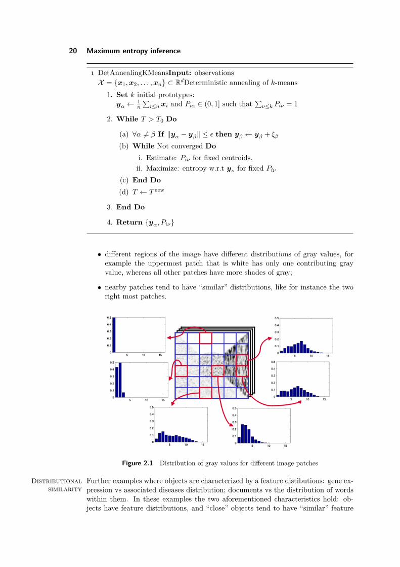
2.7.1 Distributional dataFigure 2.1 shows an image that has been divided in multiple patches, and for eachof them the distribution of gray values has been calculated. Two important charac-teristics of the obtained results can be observed:
20 Maximum entropy inference
1 DetAnnealingKMeansInput: observationsX = x1,x2, . . . ,xn ⊂ RdDeterministic annealing of k-means
1. Set k initial prototypes:yα ← 1
n
∑i≤n xi and Piα ∈ (0, 1] such that
∑ν≤k Piν = 1
2. While T > T0 Do
(a) ∀α 6= β If ‖yα − yβ‖ ≤ ε then yβ ← yβ + ξβ
(b) While Not converged Doi. Estimate: Piν for fixed centroids.ii. Maximize: entropy w.r.t yν for fixed Piν
(c) End Do(d) T ← T new
3. End Do
4. Return yα, Piν
• different regions of the image have different distributions of gray values, forexample the uppermost patch that is white has only one contributing grayvalue, whereas all other patches have more shades of gray;
• nearby patches tend to have “similar” distributions, like for instance the tworight most patches.
Figure 2.1 Distribution of gray values for different image patches
Distributionalsimilarity
Further examples where objects are characterized by a feature distibutions: gene ex-pression vs associated diseases distribution; documents vs the distribution of wordswithin them. In these examples the two aforementioned characteristics hold: ob-jects have feature distributions, and “close” objects tend to have “similar” feature
2.7 Clustering distributional data 21
distributions. The importance of this observation is that non-metric data can alsobe used to define similarity and closeness between objects, allowing to group similarobjects together.
2.7.2 Histogram clustering cost functionWe assume a generative model for histograms as follows. Distributional data can beencoded in what is known as Dyaddyads: if there are n different objects xi in the objectspace X and m possible feature values yj from the feature space Y, then a dyad isa pair (xi, yj) ∈ X×Y. Further, Dyadic datadata is a set of l observations Z = (xi(r), yj(r))lr=1.Notice that Z contains information of how often feature value yj is associated withobject xi.
Remark: in the case of Figure 2.1, objects are patches, i.e. groups of pixels, andfeature values are levels of gray. To declutter the notation, we will further denoteobject xi as i, and feature value yj as j.
For the generative model it will be assumed that random observations (i, j) comefrom different clusters indexed by α. Thus, observations are distributed accordingto some distribution
(i, j) ∼ P((i, j) | c(i), Q(j|c(i))
)(2.60)
where c(i) denotes the cluster to which object i belongs and q(j|α) is a modelprobability that describes the feature distribution given the cluster α. It is furtherassumed that the data can be synthesized by first choosing an object xi ∈ X with auniform distribution, then the cluster membership is selected according to c(i) andfinally the feature yi ∈ Y is taken from the conditional distribution Q(j|c(i)).
Remark: the final goal of the steps described below is to infer the generativehistograms. They can be seen as centroids in the space of histograms, which bringsa flavour of k-maens clustering. In order to fulfil the task we will use empiricalposterior probabilities defined below.
Under the previous assumptions, the likelihood of the data Z is given by
L(Z) =∏i≤n
∏j≤m
P ((i, j) | c(i), Q)lP (i,j), (2.61)
where lP (i, j) is the number of times object i exhibits feature value j, and P (i, j)is the empirical probability of finding object i with feature value j. P (i, j) can bewritten as
P (i, j) = 1l
∑r≤l
δi,i(r)δj,j(r), (2.62)
with δi,j being the Kronecker delta function. From the likelihood (2.61) the costfunction for the histogram clustering is defined as the negative log-likelihood of thedata
Rhc(c,Q,Z) = − log(L) = −∑i≤n
∑j≤m
lP (i, j) logP ((i, j)|c(i), q). (2.63)
To proceed further, it will be assumed that
P ((i, j) | c(i), q) = Q(j | c(i))P (c(i)).
22 Maximum entropy inference
Then, P (i, j) will be decomposed as P (i, j) = P (j|i)P (i) where
P (i) =∑j≤m
1l
∑r≤l
δi,i(r)δj,j(r), (2.64)
is the marginal distribution of P (i, j). Additionally, the data dependent but constantterm
l∑i≤n
∑j≤m
P (j|i)P (i) log(P (j|i)) (2.65)
is added to Rch. Observe that (2.65) is nothing but a multiple of the conditionalentropy of the features distribution given the objects. Since (2.65) does not dependon the assignments c or the model probabilities q it does not affect the location ofthe minimum of Rhc. The result is then
Rhc → Rhc + l∑i≤n
∑j≤m
P (j|i)P (i) log P (j|i)
= l∑i≤n
P (i)∑j≤m
P (j|i)(log P (j|i)− logQ(j|c(i))
)−l∑i≤n
∑j≤m
P (j|i)P (i) log(p(c(i)))
= l∑i≤n
P (i)∑j≤m
P (j|i) log(
P (j|i)Q(j|c(i))
)︸ ︷︷ ︸
DKL(P (·|i)‖Q(·|c(i))
)−l∑i≤n
P (i) logP (c(i))
= l∑i≤n
P (i)DKL
(P (·|i)‖Q(·|c(i))
)− l
∑i≤n
P (i) logP (c(i)). (2.66)
If a uniform distribution for the cluster membership, p(c(i)) = 1k , is assumed (2.66)
can be written as
Rhc = l∑i≤n
P (i)DKL
(P (·|i)‖Q(·|c(i))
)+ l log k (2.67)
where the Kullback-Leibler divergence1, DKL(P(·|i)‖Q(·|c(i)
), is a measure of sim-
ilarity between probability distributions. Finally, the term l log k can be dropped,and P (i) can be approximated as 1/n since the objects are drawn from a uniformdistribution. (2.67) simplifies to
Rhc(c, q) = l
n
∑i≤n
DKL
(P (·|i)‖Q(·|c(i)
). (2.68)
2.7.3 Analogy between k-means and histogram clustering
Given equation (2.68), the distributional data clustering and k-means problems canbe seen to be very similar. Observe that the cost functions are defined by a sum of“distances” from the object “feature vector” to a prototypical centroid and secondthat the cluster assignments c(i) appear linearly.
1For more details on the Kullback-Leibler divergence see Chapter 4
2.7 Clustering distributional data 23
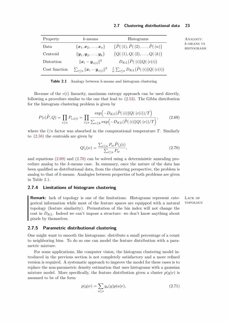
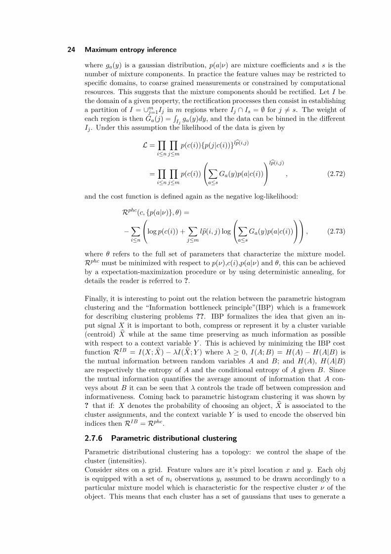
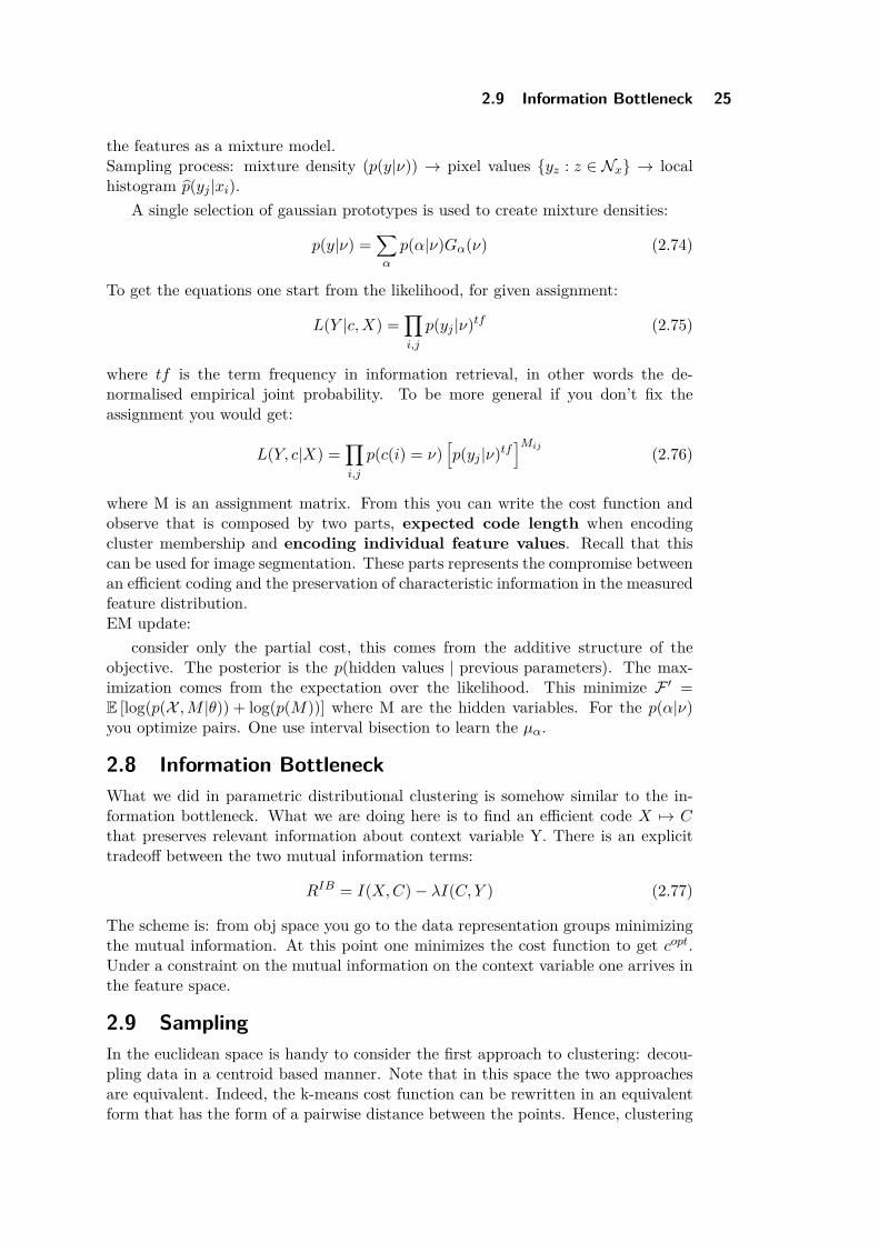
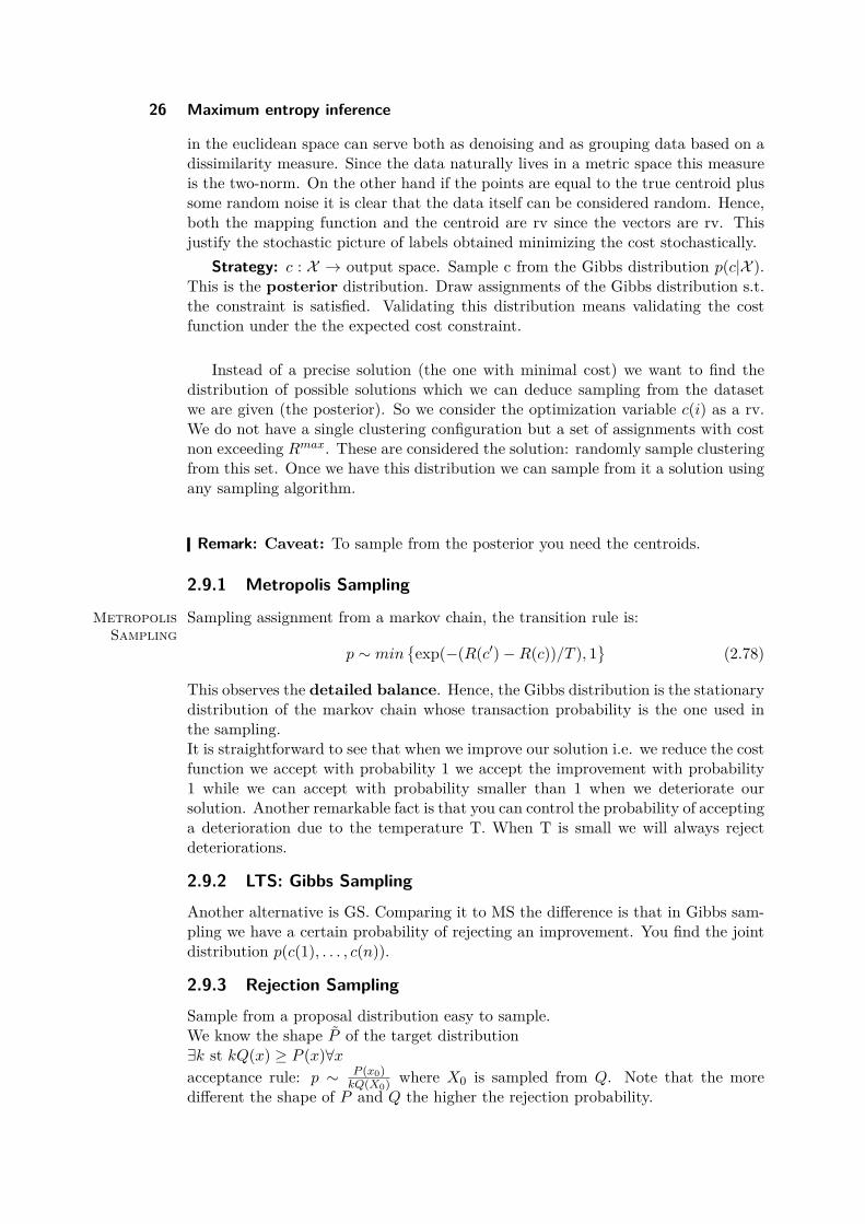
Analogy:k-means vshistograms
Property k-means Histograms
Data x1,x2, . . . ,xnP (·|1), P (·|2), . . . , P (·|n)
Centroid y1,y2, . . . ,yk
Q(·|1), Q(·|2), . . . , Q(·|k)
Distortion ‖xi − yc(i)‖2 DKL
(P (·|i)‖Q(·|c(i)
)Cost function
∑i≤n ‖xi − yc(i)‖2 l
n
∑i≤nDKL
(P (·|i)‖Q(·|c(i)
)Table 2.1 Analogy between k-means and histogram clustering
Because of the c(i) linearity, maximum entropy approach can be used directly,following a procedure similar to the one that lead to (2.53). The Gibbs distributionfor the histogram clustering problem is given by
P (c|P , Q) =∏i≤n
Pi,c(i) =∏i≤n
exp(−DKL(P (·|i)‖Q(·|c(i))/T
)∑ν≤k exp
(−DKL(P (·|i)‖Q(·|ν))/T
) , (2.69)
where the l/n factor was absorbed in the computational temperature T . Similarlyto (2.58) the centroids are given by
Q(j|ν) =∑i≤n PiνP (j|i)∑
i≤n Piν, (2.70)
and equations (2.69) and (2.70) can be solved using a deterministic annealing pro-cedure analog to the k-means case. In summary, once the nature of the data hasbeen qualified as distributional data, from the clustering perspective, the problem isanalog to that of k-means. Analogies between properties of both problems are givenin Table 2.1.
2.7.4 Limitations of histogram clustering
Remark: Lack oftopology
lack of topology is one of the limitations. Histograms represent cate-gorical information while most of the feature spaces are equipped with a naturaltopology (feature similarity). Permutation of the bin index will not change thecost in DKL. Indeed we can’t impose a structure: we don’t know anything aboutpixels by themselves.
2.7.5 Parametric distributional clusteringOne might want to smooth the histograms: distribute a small percentage of a countto neighboring bins. To do so one can model the feature distribution with a para-metric mixture.
For some applications, like computer vision, the histogram clustering model in-troduced in the previous section is not completely satisfactory and a more refinedversion is required. A systematic approach to improve the model for these cases is toreplace the non-parametric density estimation that uses histograms with a gaussianmixture model. More specifically, the feature distribution given a cluster p(y|ν) isassumed to be of the form
p(y|ν) =∑a≤s
ga(y)p(a|ν), (2.71)
24 Maximum entropy inference
where ga(y) is a gaussian distribution, p(a|ν) are mixture coefficients and s is thenumber of mixture components. In practice the feature values may be restricted tospecific domains, to coarse grained measurements or constrained by computationalresources. This suggests that the mixture components should be rectified. Let I bethe domain of a given property, the rectification processes then consist in establishinga partition of I = ∪mj=1Ij in m regions where Ij ∩ Is = ∅ for j 6= s. The weight ofeach region is then Ga(j) =
∫Ijga(y)dy, and the data can be binned in the different
Ij . Under this assumption the likelihood of the data is given by
L =∏i≤n
∏j≤m
p(c(i))p(j|c(i))lp(i,j)
=∏i≤n
∏j≤m
p(c(i))
∑a≤s
Ga(y)p(a|c(i))
lp(i,j) , (2.72)
and the cost function is defined again as the negative log-likelihood:
Rphc(c, p(a|ν), θ) =
−∑i≤n
log p(c(i)) +∑j≤m
lp(i, j) log
∑a≤s
Ga(y)p(a|c(i))
, (2.73)
where θ refers to the full set of parameters that characterize the mixture model.Rphc must be minimized with respect to p(ν),c(i),p(a|ν) and θ, this can be achievedby a expectation-maximization procedure or by using deterministic annealing, fordetails the reader is referred to ?.
Finally, it is interesting to point out the relation between the parametric histogramclustering and the “Information bottleneck principle”(IBP) which is a frameworkfor describing clustering problems ??. IBP formalizes the idea that given an in-put signal X it is important to both, compress or represent it by a cluster variable(centroid) X while at the same time preserving as much information as possiblewith respect to a context variable Y . This is achieved by minimizing the IBP costfunction RIB = I(X; X) − λI(X;Y ) where λ ≥ 0, I(A;B) = H(A) − H(A|B) isthe mutual information between random variables A and B; and H(A), H(A|B)are respectively the entropy of A and the conditional entropy of A given B. Sincethe mutual information quantifies the average amount of information that A con-veys about B it can be seen that λ controls the trade off between compression andinformativeness. Coming back to parametric histogram clustering it was shown by? that if: X denotes the probability of choosing an object, X is associated to thecluster assignments, and the context variable Y is used to encode the observed binindices then RIB = Rphc.
2.7.6 Parametric distributional clusteringParametric distributional clustering has a topology: we control the shape of thecluster (intensities).Consider sites on a grid. Feature values are it’s pixel location x and y. Each objis equipped with a set of ni observations yi assumed to be drawn accordingly to aparticular mixture model which is characteristic for the respective cluster ν of theobject. This means that each cluster has a set of gaussians that uses to generate a
2.9 Information Bottleneck 25
the features as a mixture model.Sampling process: mixture density (p(y|ν)) → pixel values yz : z ∈ Nx → localhistogram p(yj |xi).
A single selection of gaussian prototypes is used to create mixture densities:
p(y|ν) =∑α
p(α|ν)Gα(ν) (2.74)
To get the equations one start from the likelihood, for given assignment:
L(Y |c,X) =∏i,j
p(yj |ν)tf (2.75)
where tf is the term frequency in information retrieval, in other words the de-normalised empirical joint probability. To be more general if you don’t fix theassignment you would get:
L(Y, c|X) =∏i,j
p(c(i) = ν)[p(yj |ν)tf
]Mij (2.76)
where M is an assignment matrix. From this you can write the cost function andobserve that is composed by two parts, expected code length when encodingcluster membership and encoding individual feature values. Recall that thiscan be used for image segmentation. These parts represents the compromise betweenan efficient coding and the preservation of characteristic information in the measuredfeature distribution.EM update:
consider only the partial cost, this comes from the additive structure of theobjective. The posterior is the p(hidden values | previous parameters). The max-imization comes from the expectation over the likelihood. This minimize F ′ =E [log(p(X ,M |θ)) + log(p(M))] where M are the hidden variables. For the p(α|ν)you optimize pairs. One use interval bisection to learn the µα.
2.8 Information BottleneckWhat we did in parametric distributional clustering is somehow similar to the in-formation bottleneck. What we are doing here is to find an efficient code X 7→ Cthat preserves relevant information about context variable Y. There is an explicittradeoff between the two mutual information terms:
RIB = I(X,C)− λI(C, Y ) (2.77)
The scheme is: from obj space you go to the data representation groups minimizingthe mutual information. At this point one minimizes the cost function to get copt.Under a constraint on the mutual information on the context variable one arrives inthe feature space.
2.9 SamplingIn the euclidean space is handy to consider the first approach to clustering: decou-pling data in a centroid based manner. Note that in this space the two approachesare equivalent. Indeed, the k-means cost function can be rewritten in an equivalentform that has the form of a pairwise distance between the points. Hence, clustering
26 Maximum entropy inference
in the euclidean space can serve both as denoising and as grouping data based on adissimilarity measure. Since the data naturally lives in a metric space this measureis the two-norm. On the other hand if the points are equal to the true centroid plussome random noise it is clear that the data itself can be considered random. Hence,both the mapping function and the centroid are rv since the vectors are rv. Thisjustify the stochastic picture of labels obtained minimizing the cost stochastically.
Strategy: c : X → output space. Sample c from the Gibbs distribution p(c|X ).This is the posterior distribution. Draw assignments of the Gibbs distribution s.t.the constraint is satisfied. Validating this distribution means validating the costfunction under the the expected cost constraint.
Instead of a precise solution (the one with minimal cost) we want to find thedistribution of possible solutions which we can deduce sampling from the datasetwe are given (the posterior). So we consider the optimization variable c(i) as a rv.We do not have a single clustering configuration but a set of assignments with costnon exceeding Rmax. These are considered the solution: randomly sample clusteringfrom this set. Once we have this distribution we can sample from it a solution usingany sampling algorithm.
Remark: Caveat: To sample from the posterior you need the centroids.
2.9.1 Metropolis Sampling
MetropolisSampling
Sampling assignment from a markov chain, the transition rule is:
p ∼ minexp(−(R(c′)−R(c))/T ), 1
(2.78)
This observes the detailed balance. Hence, the Gibbs distribution is the stationarydistribution of the markov chain whose transaction probability is the one used inthe sampling.It is straightforward to see that when we improve our solution i.e. we reduce the costfunction we accept with probability 1 we accept the improvement with probability1 while we can accept with probability smaller than 1 when we deteriorate oursolution. Another remarkable fact is that you can control the probability of acceptinga deterioration due to the temperature T. When T is small we will always rejectdeteriorations.
2.9.2 LTS: Gibbs Sampling
Another alternative is GS. Comparing it to MS the difference is that in Gibbs sam-pling we have a certain probability of rejecting an improvement. You find the jointdistribution p(c(1), . . . , c(n)).
2.9.3 Rejection Sampling
Sample from a proposal distribution easy to sample.We know the shape P of the target distribution∃k st kQ(x) ≥ P (x)∀xacceptance rule: p ∼ P (x0)
kQ(X0) where X0 is sampled from Q. Note that the moredifferent the shape of P and Q the higher the rejection probability.
2.9 Sampling 27
2.9.4 Importance samplingNeed proposal distribution Q easy to sampleNeed to know the target distribution!!!! Sample L points from Q, compute theweights as wi = p(zi)/q(zi)∑
jp(zj)/q(zj)
. Sample again from the set according to the newweights.idea: I will resample more likely points with larger p(x).
Remark: The variance of the weights is much higher the more Q is different fromP because the reweight is heavier.
2.9.5 Compute probabilistic centroids and soft assignmentThe metropolis sampling is particularly interesting: the posterior distribution is theGibbs distribution with all the properties presented in the previous chapter. Onthe other hands for k-means you do not need a sampling strategy from the poste-rior. first: Compute Gibbs distribution P (c,Yα)for k-means. Since centroids areindependent (linear dependance in the centroid in the cost) the gibbs distribution istractable.second: find yα = argmaxyαH(c,Y) under the constraint that expected cost isbounded, take derivative to get constraint equation.third: compute derivative of previous point to get optimal centroid. Pi,α is theprobabilistic assignment defining a soft partition.
The iterative solution in EM resembles the iterative updates of k-means. Rationale:
• entropy determines the expectation values for the assignment of data to clusterand expectation values for cluster parameters (i.e. centroids)
• rather than sampling assignments as in Metropolis we calculate averages overprobable clusters with bounded expected cost.

28 Maximum entropy inference
Chapter 3
Graph based clustering
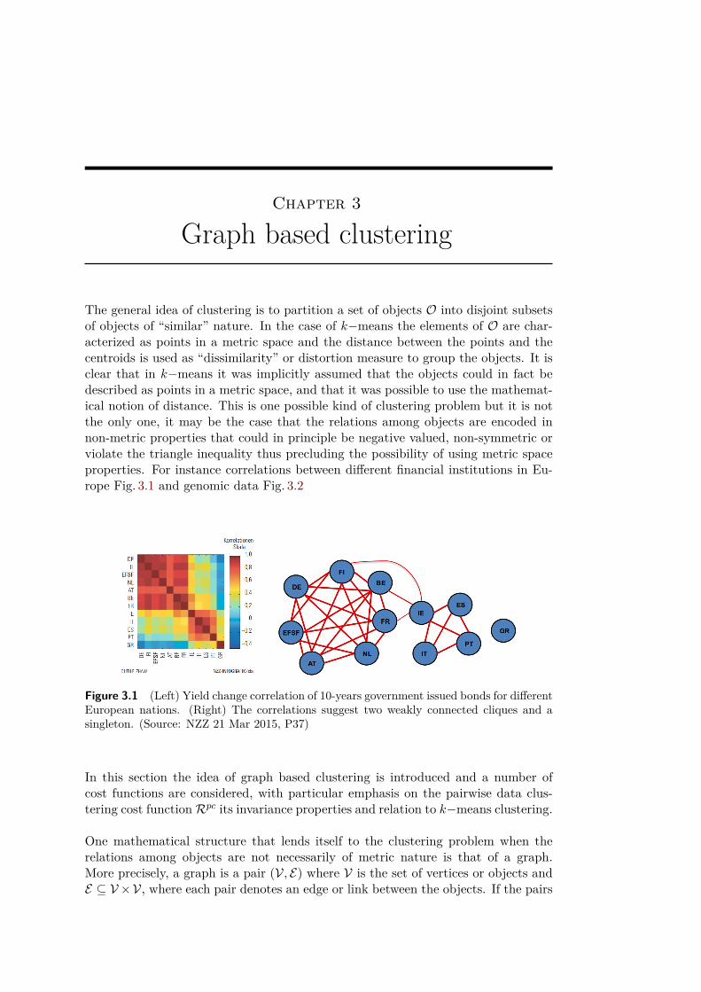
The general idea of clustering is to partition a set of objects O into disjoint subsetsof objects of “similar” nature. In the case of k−means the elements of O are char-acterized as points in a metric space and the distance between the points and thecentroids is used as “dissimilarity” or distortion measure to group the objects. It isclear that in k−means it was implicitly assumed that the objects could in fact bedescribed as points in a metric space, and that it was possible to use the mathemat-ical notion of distance. This is one possible kind of clustering problem but it is notthe only one, it may be the case that the relations among objects are encoded innon-metric properties that could in principle be negative valued, non-symmetric orviolate the triangle inequality thus precluding the possibility of using metric spaceproperties. For instance correlations between different financial institutions in Eu-rope Fig. 3.1 and genomic data Fig. 3.2
Figure 3.1 (Left) Yield change correlation of 10-years government issued bonds for differentEuropean nations. (Right) The correlations suggest two weakly connected cliques and asingleton. (Source: NZZ 21 Mar 2015, P37)
In this section the idea of graph based clustering is introduced and a number ofcost functions are considered, with particular emphasis on the pairwise data clus-tering cost functionRpc its invariance properties and relation to k−means clustering.
One mathematical structure that lends itself to the clustering problem when therelations among objects are not necessarily of metric nature is that of a graph.More precisely, a graph is a pair (V, E) where V is the set of vertices or objects andE ⊆ V ×V, where each pair denotes an edge or link between the objects. If the pairs
30 Graph based clustering
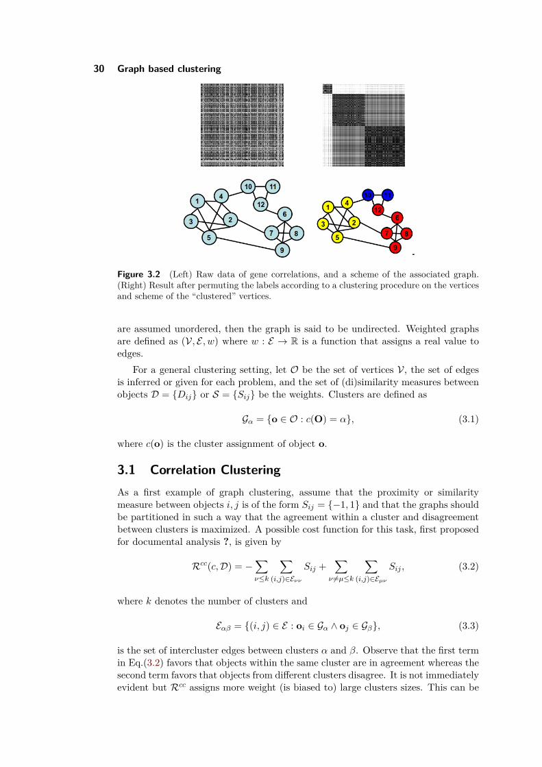
Figure 3.2 (Left) Raw data of gene correlations, and a scheme of the associated graph.(Right) Result after permuting the labels according to a clustering procedure on the verticesand scheme of the “clustered” vertices.
are assumed unordered, then the graph is said to be undirected. Weighted graphsare defined as (V, E , w) where w : E → R is a function that assigns a real value toedges.
For a general clustering setting, let O be the set of vertices V, the set of edgesis inferred or given for each problem, and the set of (di)similarity measures betweenobjects D = Dij or S = Sij be the weights. Clusters are defined as
Gα = o ∈ O : c(O) = α, (3.1)
where c(o) is the cluster assignment of object o.
3.1 Correlation ClusteringAs a first example of graph clustering, assume that the proximity or similaritymeasure between objects i, j is of the form Sij = −1, 1 and that the graphs shouldbe partitioned in such a way that the agreement within a cluster and disagreementbetween clusters is maximized. A possible cost function for this task, first proposedfor documental analysis ?, is given by
Rcc(c,D) = −∑ν≤k
∑(i,j)∈Eνν
Sij +∑
ν 6=µ≤k
∑(i,j)∈Eµν
Sij , (3.2)
where k denotes the number of clusters and
Eαβ = (i, j) ∈ E : oi ∈ Gα ∧ oj ∈ Gβ, (3.3)
is the set of intercluster edges between clusters α and β. Observe that the first termin Eq.(3.2) favors that objects within the same cluster are in agreement whereas thesecond term favors that objects from different clusters disagree. It is not immediatelyevident but Rcc assigns more weight (is biased to) large clusters sizes. This can be
3.3 Pairwise data clustering 31
seen by considering the following
Rcc(c,D) = −∑ν≤k
∑(i,j)∈Eνν
Sij +∑
ν 6=µ≤k
∑(i,j)∈Eµν
Sij ,
= −2∑ν≤k
∑(i,j)∈Eνν
Sij +∑ν,µ≤k
∑(i,j)∈Eµν
Sij ,
= −2∑ν≤k
∑(i,j)∈Eνν
Sij +∑
(i,j)∈ESij . (3.4)
Notice that the second term of Eq. (3.4) is independent of the assignment c as itis a sum over all edges. Since Gibbs distribution is invariant under constant shiftsof the cost function, the first term of Eq. (3.4) is the meaningful one. Because−2∑ν≤k
∑(i,j)∈Eνν Sij is a sum only over intracluster edges the larger the cluster
the higher its weight, which is expected to scale as the size of the cluster squared|G|2. Therefore it tends to be less expensive to add a new nodes to the bigger clustersthan to smaller ones.
A similar cost function to Eq. (3.2) is
Rgp(c,D) =∑ν≤k
∑(i,j)∈Eνν
Dij (3.5)
where the dissimilarities Dij ∈ R, this cost function has the same kind of deficienciesof Eq. (3.2) and in general is known to be bias towards very unbalanced cluster sizesi.e very large or very small.
3.2 Pairwise data clusteringA natural principle for exploratory data analysis is that of minimizing the pair-wise distances between the members within each cluster. A cost function that isconstructed to follow this idea is the pairwise clustering cost function
Rpc(c,D) = 12∑ν≤k
|Gν | ∑(i,j)∈Eνν
Dij
|Eνν |
, (3.6)
whereDij is the dissimilarity matrix and is only assumed to have zero self-dissimilarityentries, |Gν | and |Eνν | are respectively the cardinalities of the cluster Gν and its setof edges Eνν . As it will be shown below, this cost function is invariant under sym-metrization of the dissimilarity matrix and also under constant additive shifts of thenon diagonal elements. These two properties will be used to show that it is possi-ble to embed a given nonmetric proximity data problem in a vector space withoutchanging the underlying properties of the data using the “constant shift embedding”? procedure. To reach this result first it will be shown that the k−means cost func-tion Eq. (2.49) can be written in the form of Rpc, then the invariance properties ofRpc will be derived and used to establish the “constant shift embedding” procedurethat is the main result of this section.
3.3 Pairwise clustering as k-means clustering in kernel spaceIn order to show that Rkm can be seen as a special case of Rpc it is convenient torewrite Eq. (3.6) as
Rpc(c,D) = 12∑ν≤k
∑i≤n
∑j≤nMiνMjνDij∑l≤nMlν
, (3.7)
32 Graph based clustering
where Miν is a n × k matrix with entries 0 or 1 depending on whether or not theobject i is assigned to cluster ν. Notice that
∑ν≤kMiν = 1 meaning that a given
object i can only be assigned to a single cluster and∑i≤nMiν = |Gν | = nν . Now
Eq. (2.49) can be cast in the following form:
Rkm =∑i≤n||xi − yc(i)||2 =
∑ν≤ k
∑i:c(i)=ν
||xi − yν ||2 =∑ν≤ k
∑i≤n
Miν ||xi − yν ||2, (3.8)
using the definition of yν Eq. (2.51) and the identity xi ·xj = 12x
2i + 1
2x2j− 1
2 ||xi−xj ||2
it can be shown that
||xi − yν ||2 = 1nν
∑j≤n
Mjν ||xi − xj ||2 −1
2n2ν
∑j≤n
∑l≤n
MjνMlν ||xj − xl||2. (3.9)
Finally observe that if Eq.(3.9) is multiplied by Miν and then summed over allobjects the result is∑
i≤nMiν ||xi − yν ||2 = 1
2nν
∑j≤n
∑l≤n
MjνMlν ||xj − xl||2. (3.10)
Substitution of Eq. (3.10) in Eq. (3.8) yields
Rkm = 12∑ν≤k
∑j≤n
∑l≤n
MjνMlν ||xj − xl||2∑i≤nMiν
. (3.11)
It is clear that if the identification Dij = ||xi−xj ||2 is done, thenRkm can be reducedto Rpc. The previous transformation can always be carried out but the reverse notnecessarily, this is because the dissimilarity matrix may have negative values or setsof values that violate the triangle inequality making it impossible to interpret thedata as distances in a metric space.
The invariance property of Rpc under the simmetrization of the dissimilarity matrixmeans that given D, the problems Rpc(D) and Rpc(D) where D = 1
2(D + DT ) arethe same. To see this, just notice that the expression
∑i≤n
∑j≤nMiνMjνDij in the
numerator of Eq. (3.7) always has both terms Dij and Dji, thus if D is used insteadof D the result is the same due to the factor 1/2 in the definition of D.
Rpc is invariant (up to a constant) under additive shifts of the non diagonal ele-ments of D i.e. Dij → Dij = Dij + d(1− δij), this can be seen as follows
Rpc(D) = 12∑ν≤k
∑i≤n
∑j≤nMiνMjνDij + d(1− δij)∑
l≤nMlν
= Rpc(D) + 12∑ν≤k
∑i≤n
∑j≤nMiνMjνd(1− δij)∑
l≤nMlν
= Rpc(D) + d
2∑ν≤k
(nν − 1)
= Rpc(D) + d
2(n− k) (3.12)
Since the minimization problem is insensitive to overall additive constants Rpc andRpc(D) are indeed equivalent. The last idea required to build the constant shift
3.3 Pairwise clustering as k-means clustering in kernel space 33
embedding is that of the centralized version of a matrix. Let Uij(n) = 1 be an × n matrix with all its entries equal to 1, In the (n × n) identity matrix andQ = In− 1
nU(n). The centralized version of a matrix P is defined as P c = QPQ, incomponents it reads:
P cij = Pij −1n
∑k≤n
Pik −1n
∑k≤n
Pkj + 1n2
∑k,l≤n
Pkl. (3.13)
Given the symmetrization invariance of Rpc there is no loss of generality if thedissimilarity matrix is assumed symmetric from now on. Let S be a symmetricmatrix such that
Dij = Sii + Sjj − 2Sij . (3.14)
By construction D is symmetric and its diagonal elements are all zero, but S isnot unique because there are (n2 − n)/2 equations and (n2 + n)/2 variables. Eventhough S is not unique, it is the case that all S have the same centralized version Sc,and that Sc is also a valid decomposition. These statements are proven in Lemma3.and Lemma4.
Lemma 3 (Sc = −12D
c for any S that decompose D as in Eq.(3.14)). Let S be asymmetric matrix that satisfies the decomposition Eq.(3.14) for a given dissimilar-ity matrix D. Using both Eq.(3.13) and Eq. (3.14), the centralized version of S iscalculated as follows
Scij = −12
[(Dij − Sii − Sjj)−
1n
∑k≤n
(Dik − Sii − Skk)
− 1n
∑k≤n
(Dkj − Skk − Sjj) + 1n2
∑k,l≤n
(Dkl − Skk − Sll)]
= −12
[Dij −
1n
∑k≤n
Dik −1n
∑k≤n
Dkj + 1n2
∑k,l≤1
Dkl
]= −1
2Dcij . (3.15)
Lemma 4 (If S satisfies Eq.(3.14) so does Sc). Assume that S is a matrix thatsatisfies Eq.(3.14). Direct substitution of Sc in the right hand of Eq.(3.14) yields
Scii + Scjj − 2Scij = Sii + Sjj − 2Sij
− 1n
∑k≤n
Sik −1n
∑k≤n
Ski + 1n2
∑k,l≤n
Skl
− 1n
∑k≤n
Sjk −1n
∑k≤n
Skj + 1n2
∑k,l≤n
Skl
+ 2
+ 1n
∑k≤n
Sik + 1n
∑k≤n
Skj −1n2
∑k,l≤n
Skl.
= Dij , (3.16)
where the summation terms (middle three lines) cancel completely due to the sym-metry of S.
34 Graph based clustering
The importance of Lemma3 strives in the result that if Sc is positive semidefinite,then the elements ofD are given by squared euclidean distancesDij = ||xi−xj ||2, see??. In general Sc is not positive semidefinite, nevertheless it is possible to construct amatrix S that is positive semidefinite and that does not change the original problem.Notice that the (n × n) matrix A = A − λ(A)minIn, where λ(A)min denotes thesmallest eigenvalue of A, is positive definite (consider what happens when A acts onthe eigenvectors of A). Using this property construct the S matrix, in componentsSij = Scij − λ(Sc)minδij and use Eq. (3.14) to obtain the matrix D given by
Dij = Sii + Sjj − 2Sij= Scii + Scjj − 2Scij − 2λ(Sc)min(1− δij)= Dij − 2λ(Sc)min(1− δij). (3.17)
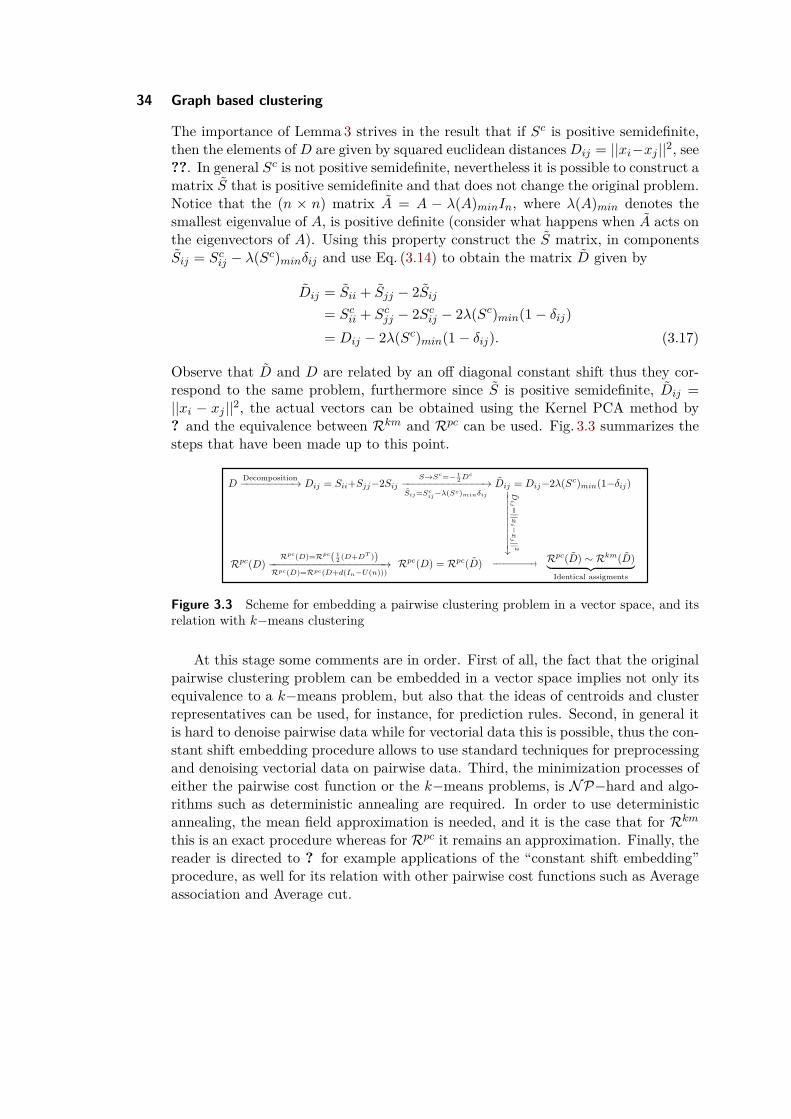
Observe that D and D are related by an off diagonal constant shift thus they cor-respond to the same problem, furthermore since S is positive semidefinite, Dij =||xi − xj ||2, the actual vectors can be obtained using the Kernel PCA method by? and the equivalence between Rkm and Rpc can be used. Fig. 3.3 summarizes thesteps that have been made up to this point.
Figure 3.3 Scheme for embedding a pairwise clustering problem in a vector space, and itsrelation with k−means clustering
At this stage some comments are in order. First of all, the fact that the originalpairwise clustering problem can be embedded in a vector space implies not only itsequivalence to a k−means problem, but also that the ideas of centroids and clusterrepresentatives can be used, for instance, for prediction rules. Second, in general itis hard to denoise pairwise data while for vectorial data this is possible, thus the con-stant shift embedding procedure allows to use standard techniques for preprocessingand denoising vectorial data on pairwise data. Third, the minimization processes ofeither the pairwise cost function or the k−means problems, is NP−hard and algo-rithms such as deterministic annealing are required. In order to use deterministicannealing, the mean field approximation is needed, and it is the case that for Rkmthis is an exact procedure whereas for Rpc it remains an approximation. Finally, thereader is directed to ? for example applications of the “constant shift embedding”procedure, as well for its relation with other pairwise cost functions such as Averageassociation and Average cut.
Chapter 4
Mean field approximation
The explicit calculation of the Gibbs distribution given a general cost function Ris not always a simple task as in the case of k−means. The problem is usually theevaluation of the partition function that involves exponentially many terms and isanalytically intractable. This often happens when the cost functions is not linearin the individual costs, or includes non trivial structures terms that make that thecost are not independent from one other. For example a local smoothness constrainterm such as
∑i≤n
∑j∈N (i) Ic(i)6=c(j) where N (j) is the neighborhood of object j.
In order to proceed, a criteria to assess the “goodness” of an approximation Qto a given distribution P is required as well as the fact that the approximation Qcan be efficiently calculated compared to the original distribution. The programto build Q is then to assume that it is of a factorial form and then minimize theKullback-Leibler divergence or relative entropy (see below) between P and Q toobtain the best factorial approximation Q of P. To carry out this program this sec-tion is organized as follows: first the Kullback-Leibler divergence is defined and itspositivity is demonstrated, afterwards the factorial approximation Q is introducedand then the minimization of the relative entropy between Q and P is explicitlycarried out.
Definition 3 (Kullback-Leibler divergence or Relative entropy). Let P(x) and Q(x)be two probability distributions defined over the same sample space Ω. The Kullback-Leibler divergence or Relative entropy is given by
D(Q||P) =∑x∈Ω
p(x) log p(x)q(x) , (4.1)
in the discrete case and
D(Q||P) =∫
Ωp(x) log p(x)
q(x)dx, (4.2)
in the continuous case.
Observe that D(Q||P) is identically zero if P = Q1, notice also that the relativeentropy is not symmetric in its arguments and that it is positive semidefinite asshow in theorem3. An intuitive but important interpretation
of the Kullback-Leibler divergence is that it quantifies the coding cost of de-scribing data with a probability distribution Q when the true distribution is P ?.Therefore its use as a comparing criteria between distributions.
1In the continuous case this holds if both distributions differ only over a set of zero measure
36 Mean field approximation
Theorem 3 (D(P||Q) is positive semidefinite). Let P(x) and Q(x) be two probabilitydistributions defined over the same sample space Ω, then
−D(P||Q) = −∑x∈Ω
p(x) log p(x)q(x) (4.3)
=∑x∈Ω
p(x) log q(x)p(x) (4.4)
≤∑x∈Ω
p(x)(q(x)p(x) − 1
)(4.5)
=∑x∈Ω
(q(x)− p(x)) = 0. (4.6)
Let Q be a factorial approximation to P given by
Q(c, θ) =∏i≤n
qi(c(i)), (4.7)
where θ is a set of free parameters, qi(ν) ∈ [0, 1] and∑ν≤k qi(ν) = 1 ∀i. Notice
that the probability of a configuration c is given by the probability of the individualassignments qi(c(i)) and that there are no correlations between the assignments ofdifferent objects.
For convenience during the minimization process the explicit dependence of theprobability distribution and cost function on the data is omitted. The Gibbs distri-bution for a general cost function R(C) can be written as
P(c) = e−βR(c)∑c′∈C e
−βR(c′) = e−βR(c)
Z= exp (−β(R(c)−F)), (4.8)
where F = − 1β logZ is known as “free energy” by analogy with statistical physics.
As explained at the beginning of this section, the idea is to minimize the quantityD(Q||P) assuming that Q is of the form Eq. 4.7. By theorem 3 it holds that
0 ≤ D(Q||P) (4.9)
Introducing the explicit forms of the distributions Eq. (4.7) and Eq. (4.8) the in-equality Eq. (4.9) can be written as
0 ≤∑c∈C
∏i≤n
qi(c(i))
∑s≤n
log qs(c(s)) + βR(c)− βF
≤∑s≤n
∑c∈C
∏i≤n
qi(c(i)) log qs(c(s))
+ βEQ(R(c))− βF , (4.10)
where the last two terms in the r.h.s of Eq. (4.10) follow from the definition of ex-pectation value and the normalization of the distribution Q. In order to simplifythe first term of the r.h.s of Eq. (4.10) observe that the sum over all possible config-urations
∑c∈C can be decomposed as follows:
∑c∈C
=k∑
r1=1
∑c∈C1
r1
, (4.11)
4.0 Mean field approximation 37
where C1r1 denotes the set of mappings that specifically map the first object to the
r1 cluster.∑c∈C1
r1can be calculated in a similar way:
∑c∈C1
r1
=k∑
r2=1
∑c∈C1,2
r1,r2
, (4.12)
where C1,2r1,r2 is the set of all mappings that assign the first object to the r1 cluster
and the second to the r2 cluster. After n iterations the result is then
∑c∈C
=k∑
r1=1
k∑r2=1· · ·
k∑rn=1
∑c∈C1,2,...,n
r1,r2,...,rn
, (4.13)
where C1,2,...,nr1,r2,...,rn is the set that contains the single mapping (1, 2, . . . n) 7→ (r1, r2, . . . rn).
Using Eq. (4.13) the first term of the r.h.s of Eq. (4.10) can be written as
∑s≤n
∑c∈C
∏i≤n
qi(c(i)) log qs(c(s))
=
∑s≤n
k∑r1=1
k∑r2=1· · ·
k∑rn=1
∑c∈C1,2,...,n
r1,r2,...,rn
qi(c(i)) log qs(c(s)) =
∑s≤n
k∑r1=1
qi(r1)k∑
r2=1q2(r2) · · ·
k∑rn=1
qn(rn) log qs(rs) =
∑s≤n
k∑rs=1
qs(rs) log qs(rs) (4.14)
Thus Eq. (4.10) can be cast in the following form
F ≤ 1β
∑s≤n
∑ν≤k
qs(ν) log qs(ν) + EQ(R(c)) ≡ B(qi(ν)), (4.15)
The first term in the r.h.s of Eq. 4.15 corresponds to the scaled negative entropyof the approximate distribution, that term together with the expected cost definethe free energy of the approximate model.2 The bound B(qi(ν)) is then the freeenergy of Q and it has to be minimized with respect to the qi(ν) subject only tothe normalization constrains.
The extremality conditions of B(qi(ν)) are given by
0 = ∂
∂qu(α)
B(qi(ν)) +
∑i≤n
λi(∑ν≤k
qi(ν)− 1), (4.16)
2Starting from the definition of the entropy of a distribution S(P) = −∑
x∈Ω p(x) log p(x) andusing the form of the Gibbs distribution Eq. (4.8) it can be shown that F = − 1
βS(P) +EPR which
can be taken as a definition of free energy for any distribution.
38 Mean field approximation
where the λi are the Lagrange coefficients that are fixed by the normalization con-strains. Using the explicit form of B(qi(ν)) Eq. (4.16) takes the form
0 = ∂
∂qu(α)1β
∑s≤n
∑ν≤k
qs(ν) log qs(ν) + ∂
∂qu(α)EQ(R(c)) + λu
= 1β
(1 + log qu(α)) + ∂
∂qu(α)∑c∈C
∏i≤n
qi(c(i))R(c) + λu
= 1β
(1 + log qu(α)) +∑c∈C
∏i 6=u≤n
qi(c(i))Ic(u)=αR(c) + λu. (4.17)
The second term in the r.h.s of Eq. (4.17) is called the mean field huα and it is theexpected cost of R(c) under the constrain that object u is assigned to cluster α thatis,
huα = EQu→αR(c) =∑c∈C
∏i 6=u≤n
qi(c(i))Ic(u)=αR(c). (4.18)
Using the mean field notation, the assignment probabilities can be obtained fromEq. (4.17) as
qu(α) = exp (−1− β(huα + λu)),
and upon normalization
qu(α) = e−β(huα)∑ν≤k e
−β(huν) . (4.19)
Having established the extremality conditions Eq. (4.17), it remains to verify thatthe second variations are positive namely
∂2
∂2qu(α)2B(qi(ν)) = (βqu(α))−1 > 0. (4.20)
Eq. (4.20) implies then that an asynchronous updating scheme of the form
qNews(t) = e−β(hs(t)α)∑
ν≤k e−β(hs(t)ν) Where
hs(t)α = EQOlds(t)→α
R(c) (4.21)
where s(t) is an arbitrary site visitation scheme will converge to a local minimum ofthe approximate free energy Eq. (4.15) in the space of factorial distributions.
Some remarks are in order regarding the mean field approach. First of all, thefactorial form of Q simplifies the summation over exponentially many assignmentconfigurations kn of n objects into k clusters, to kn summations and an optimizationproblem that can be tackled with an Expectation-Minimization approach. Second,the factorial form of Q is sufficient and convenient to perform a mean field treatmentof a problem, but it is not necessary, it is sometimes possible to use distributionsthat contain correlations,tree like structures for example, that also allows for efficientcomputations.
4.0 Mean field approximation 39
ExamplesExample 4 (Smooth k−means clustering). Consider the k−means cost function(Eq.(2.49)) to which a regularizer, that favors homogeneous assignments in the localneighborhood N (i) of each object i, is added
Rskm(c) =∑i≤n||xi − yc(i)||2 + λ
2∑i≤n
∑j∈N (i)
Ic(i)6=c(j).
Observe that if objects i and j are neighbors and the assignment c allocates both ofthem to different clusters then an extra cost of λ must be payed. In order to calculatehuα = EQu→αR(c) it is useful to split Rskm(c) in to a term that contains the objectu and one that does not:
Rskm(c) = ||xu − yc(u)||2 + λ∑
j∈N (u)Ic(u)6=c(j) +R(c|u),
where R(c|u) are costs independent of the object u. huα is then given by
huα = EQu→α||xu − yc(u)||2+ EQu→αλ∑
j∈N (u)Ic(u) 6=c(j)+ EQu→αR(c|u)
The first term in the r.h.s of the previous equation can be evaluated to ||xu − yα||2,the last term is constant and independent of u so its value does not change if thecluster assignment of u, c(u), does. The second term is evaluated as follows
EQu→αλ∑
j∈N (u)Ic(u) 6=c(j) = λ
∑j∈N (u)
EQu→αIc(u) 6=c(j)
= λ∑
j∈N (u)EQu→αIα 6=c(j)
= λ∑
j∈N (u)EQu→α
∑ν 6=α≤k
Iν=c(j)
= λ∑
j∈N (u)
∑ν 6=α≤k
EQu→αIν=c(j) (∗)
In (∗), EQu→αIν=c(j) is evaluated as
EQu→αIν=c(j) =∑c∈C
∏i 6=u≤n
qi(c(i))Ic(u)=αIν=c(j).
= qj(ν)∑c∈C
∏i 6=u,j≤n
qi(c(i))Ic(u)=αIν=c(j).
= qj(ν) (∗∗)
In the previous equation, (∗∗) was obtained by using Eq.(4.13). Inserting (∗∗) in (∗)and collecting results the final form of huα is
huα = ||xu − yα||2 + λ∑
j∈N (u)
∑ν 6=α≤k
qj(ν) + EQu→αR(c|u) (4.22)

40 Mean field approximation
Chapter 5
Approximation set coding
In this chapter1, we present an approach to model validation and robust solvingcalled Approximation Set Coding.
5.1 Setting and Generative Model Assumptions5.1.1 Optimization Problem
In the setting we are going to analyze in this and the next chapters, the followingcomponents are assumed to be defined:
• Data instanceA set X of possible data instances X:
X 3 X, (5.1)
on which no further assumptions (e.g. structure, finiteness, countability) areimposed in the most general case (see below in Section 5.1.2 for possible spec-ifications of such assumptions).
• HypothesisA set C of possible solutions, or hypotheses c:
C 3 c, (5.2)
where again no further structural or finiteness assumptions are imposed.
• Objectivefunction
An objective function R(c,X) representing the value of a given solution solu-tion c for a data instance X:
R(c,X) : C × X → R. (5.3)
If not stated otherwise, we will assume a minimization (i.e. “cost”, “error” or“energy”) semantics of R(c,X) and call it a cost function.
Definition 4. OptimizationproblemP = (X , C, R).
Provided that a solution feasibility assumption is fulfilled, i.e. anysolution c ∈ C is feasible (i.e. valid) for any data instance X ∈ X , then we can saythat these three components define a valid optimization problem denoted by a tripletP = (X , C, R).
1Based on the Chapter 3 of Alexey Gronskiy’s PhD thesis (2018).
42 Approximation set coding
The optimization goal consists in finding the set of those solutions which mini-mize the cost function:
C⊥(X) := arg minc∈C
R(c,X). (5.4)
With a bit of notation abuse we will also write
c⊥(X) := arg minc∈C
R(c,X) ∈ C⊥(X), (5.5)
meaning a one (out of many possible) optimal solution (global minimizer). We willdenote the optimal cost as:
R⊥(X) := minc∈C
R(c,X). (5.6)
5.1.2 Data Generation Model
Dealing with uncertainty in optimization requires to define a data generation process.In the following, we will simply assume that there is exists true (ground, signal)
data instance X0, from which the noise-contaminated data instances are obtainedindependently, i.e.:
X ′, X ′′, X ′′′, · · · ∼ PG(X|X0) (5.7)
Problemgenerator
through a problem generating process PG(·|X0). Note that the problem generatingprocess is parametrized through the ground truth X0. Note also that the obtaineddata instances are independent, conditioned on the X0:
for any data instances X ′, X ′′ ∼ PG(X|X0): X ′ ⊥⊥ X ′′|X0. (5.8)
Remark: Although this notation might seem complex, it is actually very straight-forward. In most cases we consider, X ∈ X will be just a vector of random(generated by PG(·)) weights from which the costs R(c,X) are constructed.
5.2 Approximation Set-Based ApproachIn this section, we will introduce the notions related to Approximation Set Codingframework — a successful way of regularizing solutions to cost-driven optimizationproblems.
5.2.1 Approximation Sets
Approximationset-basedapproach
We introduce the notion of approximation sets, which are intended to address thequestion: how to avoid the risk of overfitting in those frequent cases, when the solveris not aware of precise noise conditions PG(·) imposed on the dataset?
Consider the following thought experiment: datasets X ′, X ′′, . . . are drawn ac-cording to the random data generation process PG(·|X0) as given in Section 5.1.2.As all the datasets stem from the same “ground” dataset X0 (in some sense, whichwe leave undefined for the sake of keeping things simple for now), they contain bothuseful and irrelevant information. In other words: only some information the oneobtains from the dataset “explains signal” X0 (e.g. has low condition entropy), whilethe rest of the information “explains noise”.
5.2 Approximation Set-Based Approach 43
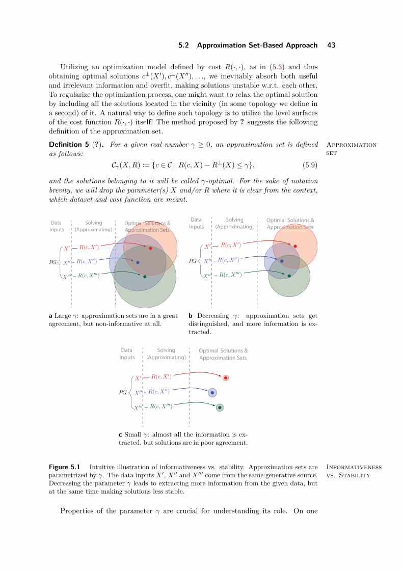
Utilizing an optimization model defined by cost R(·, ·), as in (5.3) and thusobtaining optimal solutions c⊥(X ′), c⊥(X ′′), . . ., we inevitably absorb both usefuland irrelevant information and overfit, making solutions unstable w.r.t. each other.To regularize the optimization process, one might want to relax the optimal solutionby including all the solutions located in the vicinity (in some topology we define ina second) of it. A natural way to define such topology is to utilize the level surfacesof the cost function R(·, ·) itself! The method proposed by ? suggests the followingdefinition of the approximation set.
Definition 5 (?). Approximationset
For a given real number γ ≥ 0, an approximation set is definedas follows:
Cγ(X,R) := c ∈ C | R(c,X)−R⊥(X) ≤ γ, (5.9)
and the solutions belonging to it will be called γ-optimal. For the sake of notationbrevity, we will drop the parameter(s) X and/or R where it is clear from the context,which dataset and cost function are meant.
X ′
X ′′
X ′′′
R(c,X ′)
R(c,X ′′)
R(c,X ′′′)
Data
Inputs
Solving
(Approximating)
OptimaOptimaOptimalll Solutions &Solutions &Solutions &
ApApAppproximation Setsximation Setsximation Sets
PG
a Large γ: approximation sets are in a greatagreement, but non-informative at all.
Data
Inputs
Solving
(Approximating)
Optimal Solutions &
Approoximation Setsximation Sets
X ′
X ′′
X ′′′
R(c,X ′)
R(c,X ′′)
R(c,X ′′′)
oximation Sets
PG
b Decreasing γ: approximation sets getdistinguished, and more information is ex-tracted.
Data
Inputs
Solving
(Approximating)
Optimal Solutions &
Approximation Sets
X ′
X ′′
X ′′′
PG
R(c,X ′)
R(c,X ′′)
R(c,X ′′′)
c Small γ: almost all the information is ex-tracted, but solutions are in poor agreement.
Figure 5.1 Informativenessvs. Stability
Intuitive illustration of informativeness vs. stability. Approximation sets areparametrized by γ. The data inputs X ′, X ′′ and X ′′′ come from the same generative source.Decreasing the parameter γ leads to extracting more information from the given data, butat the same time making solutions less stable.
Properties of the parameter γ are crucial for understanding its role. On one
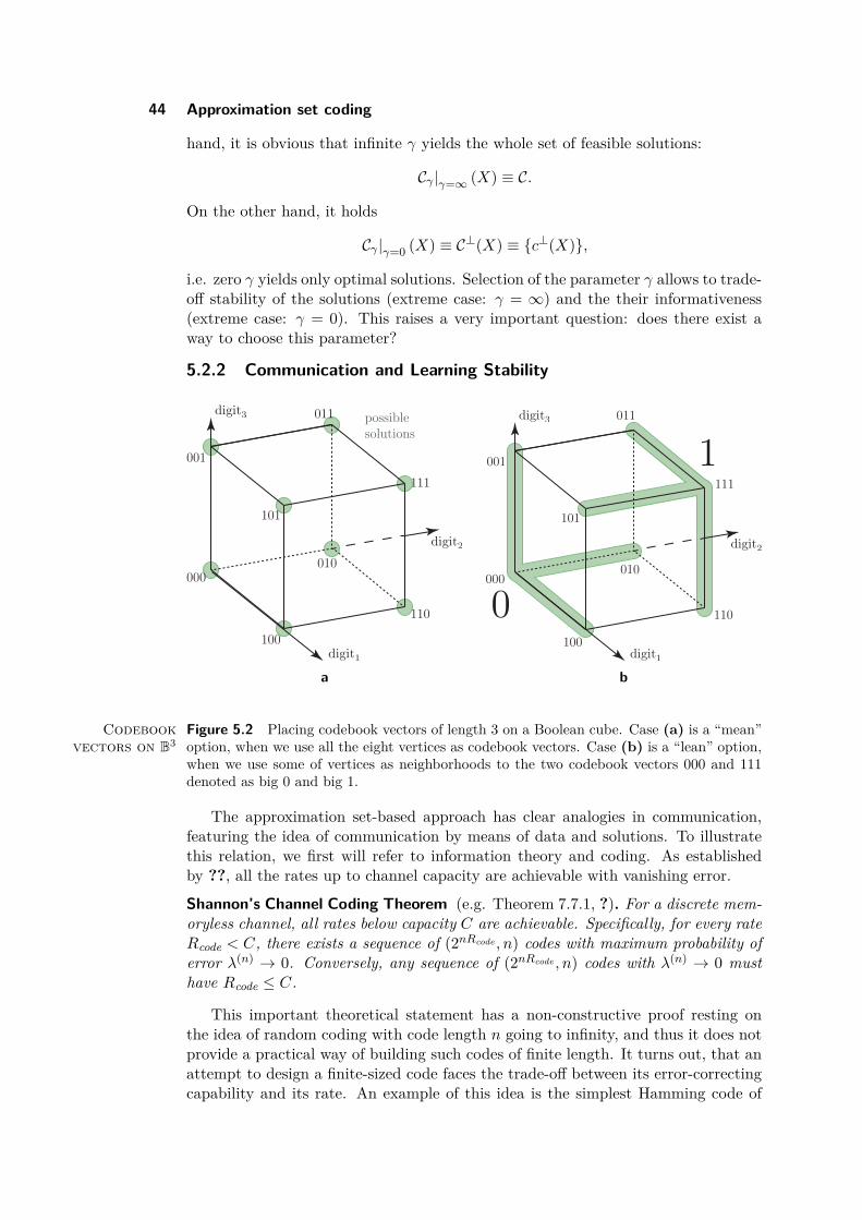
44 Approximation set coding
hand, it is obvious that infinite γ yields the whole set of feasible solutions:
Cγ |γ=∞ (X) ≡ C.
On the other hand, it holds
Cγ |γ=0 (X) ≡ C⊥(X) ≡ c⊥(X),
i.e. zero γ yields only optimal solutions. Selection of the parameter γ allows to trade-off stability of the solutions (extreme case: γ = ∞) and the their informativeness(extreme case: γ = 0). This raises a very important question: does there exist away to choose this parameter?
5.2.2 Communication and Learning Stability
000
100
110
010
111
011
101
001
possible solutions
a
000
100
110
010
111
011
101
001
0
1
b
Figure 5.2Codebookvectors on B3
Placing codebook vectors of length 3 on a Boolean cube. Case (a) is a “mean”option, when we use all the eight vertices as codebook vectors. Case (b) is a “lean” option,when we use some of vertices as neighborhoods to the two codebook vectors 000 and 111denoted as big 0 and big 1.
The approximation set-based approach has clear analogies in communication,featuring the idea of communication by means of data and solutions. To illustratethis relation, we first will refer to information theory and coding. As establishedby ??, all the rates up to channel capacity are achievable with vanishing error.
Shannon’s Channel Coding Theorem (e.g. Theorem 7.7.1, ?). For a discrete mem-oryless channel, all rates below capacity C are achievable. Specifically, for every rateRcode < C, there exists a sequence of (2nRcode , n) codes with maximum probability oferror λ(n) → 0. Conversely, any sequence of (2nRcode , n) codes with λ(n) → 0 musthave Rcode ≤ C.
This important theoretical statement has a non-constructive proof resting onthe idea of random coding with code length n going to infinity, and thus it does notprovide a practical way of building such codes of finite length. It turns out, that anattempt to design a finite-sized code faces the trade-off between its error-correctingcapability and its rate. An example of this idea is the simplest Hamming code of
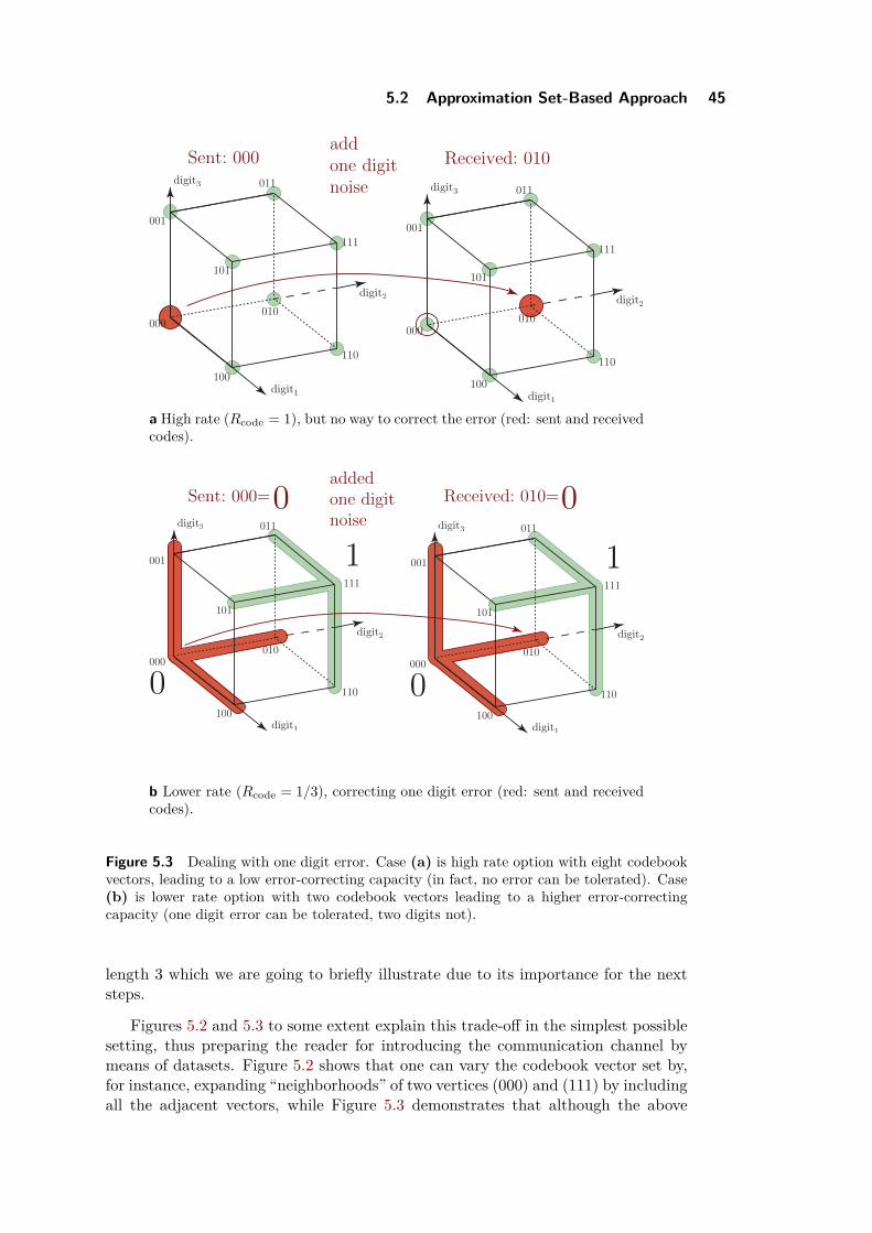
5.2 Approximation Set-Based Approach 45
000
100
110
010
111
011
101
001
000
100
110
010
111
011
101
001
Sent: 000 Received: 010addone digitnoise
a High rate (Rcode = 1), but no way to correct the error (red: sent and receivedcodes).
Sent: 000= Received: 010=
000
100
110
010
111
011
101
001
0
1
000
100
110
010
111
011
101
001
0
1
0 0added one digitnoise
b Lower rate (Rcode = 1/3), correcting one digit error (red: sent and receivedcodes).
Figure 5.3 Dealing with one digit error. Case (a) is high rate option with eight codebookvectors, leading to a low error-correcting capacity (in fact, no error can be tolerated). Case(b) is lower rate option with two codebook vectors leading to a higher error-correctingcapacity (one digit error can be tolerated, two digits not).
length 3 which we are going to briefly illustrate due to its importance for the nextsteps.
Figures 5.2 and 5.3 to some extent explain this trade-off in the simplest possiblesetting, thus preparing the reader for introducing the communication channel bymeans of datasets. Figure 5.2 shows that one can vary the codebook vector set by,for instance, expanding “neighborhoods” of two vertices (000) and (111) by includingall the adjacent vectors, while Figure 5.3 demonstrates that although the above
46 Approximation set coding
process reduces the code rate from Rcode = 1 down to Rcode = 1/3, it increases itserror-correcting capability so that the code can now tolerate all the one-digit errors.One can also imagine an extreme (not shown in figures) case of high two-digit noise:it is easy to see that under this condition, a reliable, stable communication is onlypossible with only one codebook vector and the zero rate (Rcode = 0). In otherwords, the code gets less informative, but more robust.
Algorithm 1: Establishing the CommunicationData:instance of the dataset X ′ ∈ X ,solution set C = c,cost function R(c,X),set of transformations T = τ, where τ : X → Xparameter γ
Result: established communication scheme1 Sender and Receiver agree on R(c,X);2 Sender and Receiver agree on X ′;3 Sender and Receiver agree on T;4 Sender and Receiver agree on γ;5 // Then, a coverage by approximation sets is generated:6 foreach τ ∈ T do7 both Sender and Receiver generate a transformed dataset τ X ′;8 both Sender and Receiver compute γ-approximation set Cγ(τ X ′);
Learning ascommunication
As well as in the coding scenario described above, the learning process can be viewedas a noisy communication, where the model is a decoder which tries to figure outthe solution to true (useful) signal contained in the noisy data. Thus, the followingrough analogies can be pointed out:
• The role of codebook vectors is played by solutions c to the optimizationproblem R(c,X).
• The role of errors is played by the noise generating process PG() (see. (5.7)),which injects uncertainty into data X.
• The role of “neighborhoods” of codebook vectors from Figures 5.2b and 5.3bis played by approximation sets.
We are now going, following ?, to introduce an artificial communication sce-nario (Algorithms 1, 2 and 3). We advise the reader to compare the textual expla-nation with the pictorial one in Figure. 5.4.
Encoding step (Algorithm 1 and 2; Fig. 5.4a)Sender-Receiverterminology
Very briefly, the Sender-Receiveranalogy consists in distinguishing individual solutions by means of the noisy datasets:Sender sends a message (defined below) encoded by the first dataset, and Receiverreceives this message, but perturbed by means of the second dataset. More precisely,assuming the generative process PG (see (5.7)), the transmitted “messages” are thetransformations τ ∈ T of the datasets, so
τ ∈ T, τ : X → X . (5.10)
5.2 Approximation Set-Based Approach 47
Now, both Sender and Receiver are agreeing on the dataset X ′, which will play therole of the encoding “benchmark”. Sender then picks a transformation τsend andencodes the message by means of X ′ via applying one to the other:
Xsend := τsend X ′, (5.11)
and sends it out. Remember that Receiver does not know τsend, but knows “codebookapproximation sets” τ X ′τ∈T.
Hypothetic noise-free transmission What if therewere no noise?
If there were no noise, Receiver, having obtainedXreceived = Xsend, and knowing both T and X ′, could just recover the τsend byenumerating:
τ := arg maxτ∈T
1Xreceived = τ X ′. (5.12)
Actual noisy transmission (Algorithm 2; Fig. 5.4b) However, the noise is injectedby replacing X ′ by X ′′, which is a noisy version of the initial dataset:
Xreceived := τsend X ′′, (5.13)
which makes it impossible for Receiver to perfectly match obtained message to anyof the “benchmarked ones” like in Eq. (5.12).
Remark: It it important to realize, that there are two manifestations of noise inthis scenario. One is the original source of noise generated by PG(·) and resultingin replacing X ′ by X ′′. The other is the transmission error caused by differencebetween the sent and received messages.
Decoding (Algorithm 3; Fig. 5.4c and 5.4d) Just the same as the Hammingchannel performs decoding the received vector by finding the closest codebook vec-tor, our Receiver tries to find the closest codebook dataset out of all the possible
Algorithm 2: Encoding and TransmissionData:
instance of the dataset X ′ ∈ X ,instance X ′′ ∈ X not known to receiver,solution set C = c,cost function R(c,X),set of transformations T = τ, where τ : X → Xparameter γ
Result: a received message1 Sender picks a τsend ∈ T and sends it;2 Sender encodes it by generating a transformed dataset τsend X ′ and sends
it;3 Sender sends τsend X ′;4 // Channel noise comes in the next line:5 Channel introduces error by applying transformation τsend to a X ′′;6 Receiver receives τsend X ′′ without knowing either τsend or X ′′;
48 Approximation set coding
Algorithm 3: DecodingData:instance of the dataset X ′ ∈ X ,instance X ′′ ∈ X not known to receiver,solution set C = c,cost function R(c,X),set of transformations T = τ, where τ : X → Xparameter γ
Result: Transformation τ which is estimate for τsend1 Receiver computes a γ-approximation set of the received dataset:Cγ(τsend X ′′);
2 Receiver maximizes its overlap with known γ-approximation sets:
τ = arg maxτ∈T
∣∣Cγ(τ X ′) ∩ Cγ(τsend X ′′)∣∣ (5.15)
datasets τ X ′τ∈T. Closeness is measured as the size of the intersection of theirapproximation sets:
τ = arg maxτ∈T
∣∣Cγ(τ X ′) ∩ Cγ(τsend X ′′)∣∣, (5.14)
thus, approximation sets play the role of parity check regions here.Overlap and
Hammingdecoding
It is crucially important to realize that this decoding rule is very similar to that ofthe Hamming code (and thus very natural), because in the Hamming coding, thecloseness is measured by minimizing the Hamming distance between the receivedvector and the codebook vectors, which is the same as maximizing the intersectionbetween them:
x = arg minx∈B3
‖xreceived ⊕ x‖
= arg minx∈B3
(n− ‖xreceived ∩ x‖
)= arg max
x∈B3‖xreceived ∩ x‖. (5.16)
Decoding error and its probability When τ 6= τsend, we say that a decoding erroroccurs. Obviously, the noise in our channel (Algorithm 2), acting via PG(·|X0), isthe reason for that. Transferring robust optimization problem into a robust decodingproblem, we now will answer, following ?, a natural question: how can we boundthis probability?
We are interested in bounding the probability
P(τ 6= τsend|τsend). (5.17)
Before we proceed, we will denote the intersection in (5.15) as follows:
∆Cτγ := Cγ(τ X ′) ∩ Cγ(τsend X ′′). (5.18)
Due to the union bound, it holds that
P(τ 6= τsend|τsend) ≤∑τ∈T
P(|∆Cτγ | ≥ |∆Cτsend
γ |∣∣ τsend
), (5.19)
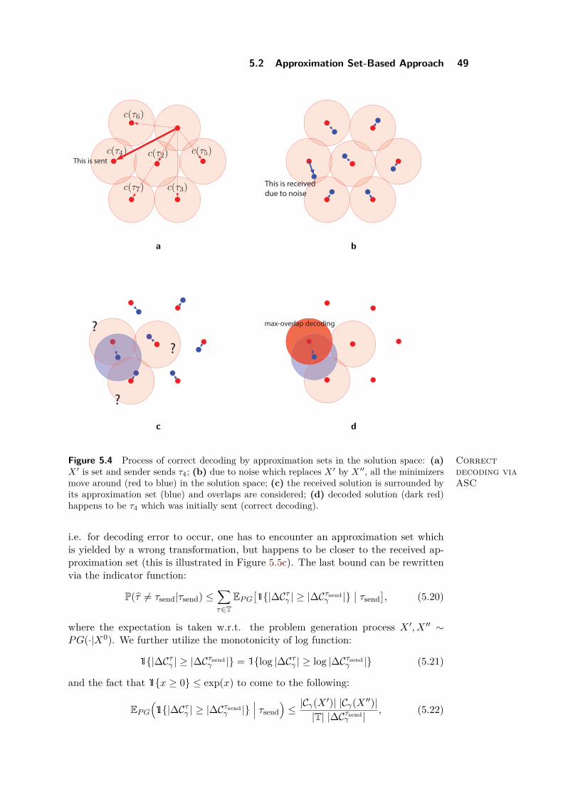
5.2 Approximation Set-Based Approach 49
c(τ2)
c(τ3)
c(τ4) c(τ5)
c(τ6)
c(τ7)
This is sent
a
This is received
due to noise
b
?
?
?
c
max-overlap decoding
d
Figure 5.4 Correctdecoding viaASC
Process of correct decoding by approximation sets in the solution space: (a)X ′ is set and sender sends τ4; (b) due to noise which replaces X ′ by X ′′, all the minimizersmove around (red to blue) in the solution space; (c) the received solution is surrounded byits approximation set (blue) and overlaps are considered; (d) decoded solution (dark red)happens to be τ4 which was initially sent (correct decoding).
i.e. for decoding error to occur, one has to encounter an approximation set whichis yielded by a wrong transformation, but happens to be closer to the received ap-proximation set (this is illustrated in Figure 5.5c). The last bound can be rewrittenvia the indicator function:
P(τ 6= τsend|τsend) ≤∑τ∈T
EPG[1|∆Cτγ | ≥ |∆Cτsend
γ |∣∣ τsend
], (5.20)
where the expectation is taken w.r.t. the problem generation process X ′, X ′′ ∼PG(·|X0). We further utilize the monotonicity of log function:
1|∆Cτγ | ≥ |∆Cτsendγ | = 1log |∆Cτγ | ≥ log |∆Cτsend
γ | (5.21)
and the fact that 1x ≥ 0 ≤ exp(x) to come to the following:
EPG(1|∆Cτγ | ≥ |∆Cτsend
γ |∣∣∣ τsend
)≤ |Cγ(X ′)| |Cγ(X ′′)|
|T| |∆Cτsendγ |
, (5.22)
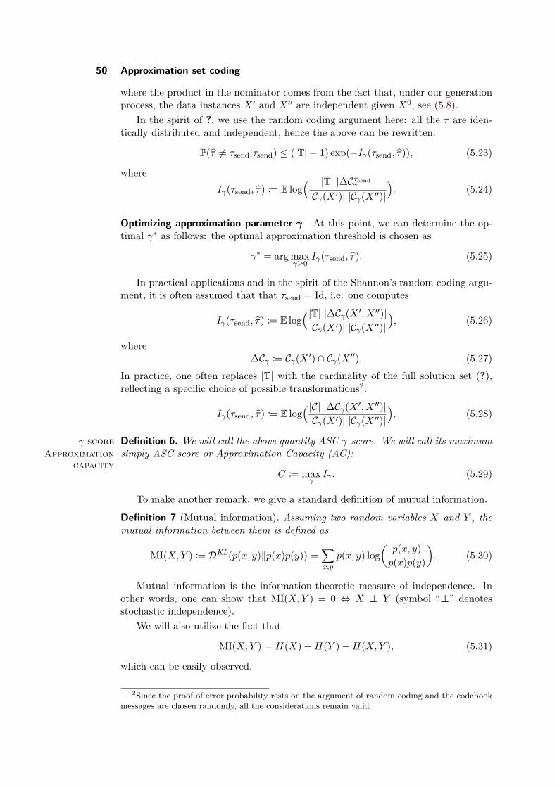
50 Approximation set coding
where the product in the nominator comes from the fact that, under our generationprocess, the data instances X ′ and X ′′ are independent given X0, see (5.8).
In the spirit of ?, we use the random coding argument here: all the τ are iden-tically distributed and independent, hence the above can be rewritten:
P(τ 6= τsend|τsend) ≤ (|T| − 1) exp(−Iγ(τsend, τ)), (5.23)
whereIγ(τsend, τ) := E log
( |T| |∆Cτsendγ |
|Cγ(X ′)| |Cγ(X ′′)|). (5.24)
Optimizing approximation parameter γ At this point, we can determine the op-timal γ∗ as follows: the optimal approximation threshold is chosen as
γ∗ = arg maxγ≥0
Iγ(τsend, τ). (5.25)
In practical applications and in the spirit of the Shannon’s random coding argu-ment, it is often assumed that that τsend = Id, i.e. one computes
Iγ(τsend, τ) := E log( |T| |∆Cγ(X ′, X ′′)||Cγ(X ′)| |Cγ(X ′′)|
), (5.26)
where∆Cγ := Cγ(X ′) ∩ Cγ(X ′′). (5.27)
In practice, one often replaces |T| with the cardinality of the full solution set (?),reflecting a specific choice of possible transformations2:
Iγ(τsend, τ) := E log( |C| |∆Cγ(X ′, X ′′)||Cγ(X ′)| |Cγ(X ′′)|
), (5.28)
Definition 6.γ-score We will call the above quantity ASC γ-score. We will call its maximumsimply ASC score or Approximation Capacity (AC):Approximation
capacityC := max
γIγ . (5.29)
To make another remark, we give a standard definition of mutual information.
Definition 7 (Mutual information). Assuming two random variables X and Y , themutual information between them is defined as
MI(X,Y ) := DKL(p(x, y)‖p(x)p(y)) =∑x,y
p(x, y) log(p(x, y)p(x)p(y)
). (5.30)
Mutual information is the information-theoretic measure of independence. Inother words, one can show that MI(X,Y ) = 0 ⇔ X ⊥⊥ Y (symbol “⊥⊥” denotesstochastic independence).
We will also utilize the fact that
MI(X,Y ) = H(X) +H(Y )−H(X,Y ), (5.31)
which can be easily observed.
2Since the proof of error probability rests on the argument of random coding and the codebookmessages are chosen randomly, all the considerations remain valid.
5.2 Approximation Set-Based Approach 51
a
b c
Figure 5.5 Incorrectdecoding viaASC
Decreased γ and increased code rate leads to incorrect decoding: (a) samesetting (i.e. same noise) as in Figure 5.4, but added more codebook vectors; (b) due tonoise which replaces X ′ by X ′′, all the minimizers move around (red to blue) in the solutionspace, (c) decoded solution (dark red) happens to be wrong (incorrect decoding).
Remark: It is interesting to note that the semantics of Iγ(τsend, τ) is surprisinglysimilar to that of mutual information (Definition 7). First, both are related tothe maximum rate of certain channel. Second, both can be decomposed in quite asimilar way: recall from (5.31) that, for random variables X and Y ,
MI(X,Y ) = H(X) +H(Y )−H(X,Y ).
In a same way one may observe, that (5.28) can be very easily decomposed intothree logarithms:
Iγ(τsend, τ) =
single entropy︷ ︸︸ ︷−E log
( |Cγ(X ′)||C|
) single entropy︷ ︸︸ ︷−E log
( |Cγ(X ′′)||C|
)+E log
( |∆Cγ(X ′, X ′′)||C|
)︸ ︷︷ ︸
joint entropy
, (5.32)
52 Approximation set coding
where first two terms can be contemplated as single entropies of uniform distribu-tions over approximation sets, and the third term corresponds to the joint entropy.
Remark: In practical applications, when there are only two data points X ′, X ′′ andno information about PG(·) is available, one can use an empirical version of (5.28)
Iγ(X ′, X ′′) := log( |C| |∆Cγ(X ′, X ′′)||Cγ(X ′)| |Cγ(X ′′)|
), (5.33)
as an estimator without the expectation sign.
Chapter 6
Probably Approximately CorrectLearning
(In draft state)A very important and common problem in statistical learning theory is that of
classification. In this scenario not only the “raw” data is given, as for k−means, butalso associated to every data point there is a label which is an element from a finiteset of options. The task is then to assign the right label to new unlabeled data pointsusing the knowledge of the previously given data (also known as training data). Onepossible approach to such a problem is that of Bayes classification in which the labelis chosen such that it maximizes the posterior probability of the label given the data.It can be shown that this labeling rule, called Bayes classifier, minimizes the prob-ability of missclassification ? and therefore is the theoretically best possible option.Nevertheless there is a caveat, the joint probability distribution of data and labelswhich is needed for the Bayes classifier is usually unknown. This implies that beforesolving the actual task it is necessary to solve a density estimation problem which isin general difficult, furthermore it can be criticized that in many cases it is unknownto what extent biases are introduced when a particular prior is chosen in the densityestimation task. The aim of the probably approximately correct (PAC) learningmodel is to provide a framework for the classification problem that is distributionindependent, thus avoiding the density estimation task, in the spirit of V.N.Vapnik“Don’t solve a harder problem than necessary”. In this section the PAC model ispresented. First the classification setting will be formalized, then the PAC model isintroduced and finally an example will be given.
The classification problem can be formalized using the following ideas: Let X de-note the instance space, that is the space that encodes the objects in the learners(algorithm) world, a concept over X is defined as a subset c ⊂ X of the instancespace or equivalently as a function c : X → 0, 1 where c(x) = 1(0) denotes a posi-tive(negative) example. A concept class is a collection of concepts. For instance Xcan be the set of all possible configurations of a pixel array and the concept class of“A” can be the subset of configurations that represent the letter A. The set of sam-ples or data is defined as a subset Z := (xi, yi) : 1 ≤ i ≤ n ⊂ X ×0, 1 where n isthe number of samples and 0, 1 is the set of labels that denotes negative or positiveexamples. Finally a classifier is a function c : X → 0, 1 from the instance spaceto the label space. When the classifier has been trained under a specific set of sam-ples it will be denoted by cn, where the n specifies the number of sample points used.
54 Probably Approximately Correct Learning
Given that the Bayes classifier cBayes is the theoretically best possible classifier,the question is then how to rate or judge the quality of classifier cn. Consider therelation between cn(X) and cBayes(X), they can be either equal or not and this willbe a random event that depends on both the distribution of the data and the partic-ular training set Z used. Because of the stochasticity of the relation between cn(X)and cBayes(X) a probabilistic approach is required and a natural option is to con-sider the so called “probability of large excess error” Pcn(X) 6= cBayes(X)|Z ≤ ε.This quantity qualifies cn as an approximately correct classifier if it does not dis-agree with the Bayes classifier in a fraction of the cases larger than ε. The issuewith this approach is that it dependents on the training data Z, and therefore it isstill random in nature.
To bypass the shortcomings of the probability of large excess error as a qualitymeasure for a trained classifier cn an (ε, δ) criteria is required. The idea is that ifwith “high probability” the performance of cn is “as close as possible” to that ofcbayes then cn is a good classifier. Formally the performance is measured by theprobability of miss classification or expected risk
R(c) = Pc(X) 6= Y, (6.1)
where c is a classifier and X, Y are the data and label random variables. The notionsof “as close as possible” and “high probability” are formalized with the ε > 0 andδ > 0 parameters as follows: if it can be shown that
PX,YR(cn) ≤ R(cBayes) + ε > 1− δ, (6.2)
then it is clear that the performance of cn will be for most of the time ( a fraction1− δ of the cases), ε close to the optimal classifier. Eq. (6.2) or its converse
PX,YR(cn) > R(cBayes) + ε < δ, (6.3)
are also useful to define the idea of “sample complexity” as the smallest sample sizeN(ε, δ) for wich Eq. (6.2) or Eq. (6.3) holds for all distributions of the data if thesample size is larger than N(ε, δ).
PAC learning
The PAC learning model is motivated by the previous ideas, but instead of consid-ering the relation between a trained classifier and the Bayes classifier, the classifieris compared against the best possible classifier within the considered concept class.The reason behind this idea, is that it may be the case that the Bayes classifier is socomplex that it is nowhere to be found in the considered set of rules and thereforean approximation is needed.
Definition 8 (Probably Approximately Correct learning). Let X be an instance spaceand C a concept class over X . The concept class C is learnable if there exists analgorithm A such that: for every concept c ∈ C, for every distribution D over X ,and for all 0 < ε < 1/2 and 0 < δ < 1/2, if A is given inputs ε, δ and access toan oracle EX(c,D) that is able to draw independent samples from X according to Dand label them according to the concept c, then with probability 1− δ the outcome ofA is a hypothesis concept h that satisfies Error(h) := R(h)− infc∈CR(c) < ε. Thisprobability is taken over the random examples of the oracle and any possible internalrandomization of A
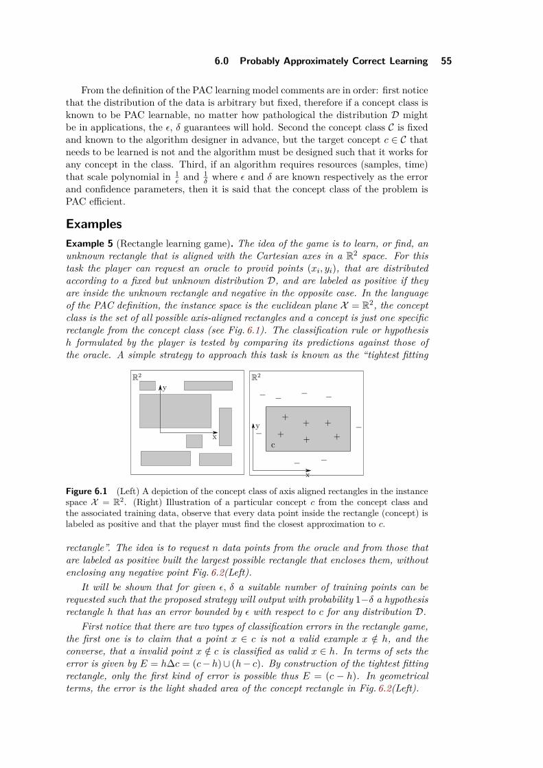
6.0 Probably Approximately Correct Learning 55
From the definition of the PAC learning model comments are in order: first noticethat the distribution of the data is arbitrary but fixed, therefore if a concept class isknown to be PAC learnable, no matter how pathological the distribution D mightbe in applications, the ε, δ guarantees will hold. Second the concept class C is fixedand known to the algorithm designer in advance, but the target concept c ∈ C thatneeds to be learned is not and the algorithm must be designed such that it works forany concept in the class. Third, if an algorithm requires resources (samples, time)that scale polynomial in 1
ε and 1δ where ε and δ are known respectively as the error
and confidence parameters, then it is said that the concept class of the problem isPAC efficient.
ExamplesExample 5 (Rectangle learning game). The idea of the game is to learn, or find, anunknown rectangle that is aligned with the Cartesian axes in a R2 space. For thistask the player can request an oracle to provid points (xi, yi), that are distributedaccording to a fixed but unknown distribution D, and are labeled as positive if theyare inside the unknown rectangle and negative in the opposite case. In the languageof the PAC definition, the instance space is the euclidean plane X = R2, the conceptclass is the set of all possible axis-aligned rectangles and a concept is just one specificrectangle from the concept class (see Fig. 6.1). The classification rule or hypothesish formulated by the player is tested by comparing its predictions against those ofthe oracle. A simple strategy to approach this task is known as the “tightest fitting
Figure 6.1 (Left) A depiction of the concept class of axis aligned rectangles in the instancespace X = R2. (Right) Illustration of a particular concept c from the concept class andthe associated training data, observe that every data point inside the rectangle (concept) islabeled as positive and that the player must find the closest approximation to c.
rectangle”. The idea is to request n data points from the oracle and from those thatare labeled as positive built the largest possible rectangle that encloses them, withoutenclosing any negative point Fig. 6.2(Left).
It will be shown that for given ε, δ a suitable number of training points can berequested such that the proposed strategy will output with probability 1−δ a hypothesisrectangle h that has an error bounded by ε with respect to c for any distribution D.
First notice that there are two types of classification errors in the rectangle game,the first one is to claim that a point x ∈ c is not a valid example x /∈ h, and theconverse, that a invalid point x /∈ c is classified as valid x ∈ h. In terms of sets theerror is given by E = h∆c = (c− h)∪ (h− c). By construction of the tightest fittingrectangle, only the first kind of error is possible thus E = (c − h). In geometricalterms, the error is the light shaded area of the concept rectangle in Fig. 6.2(Left).
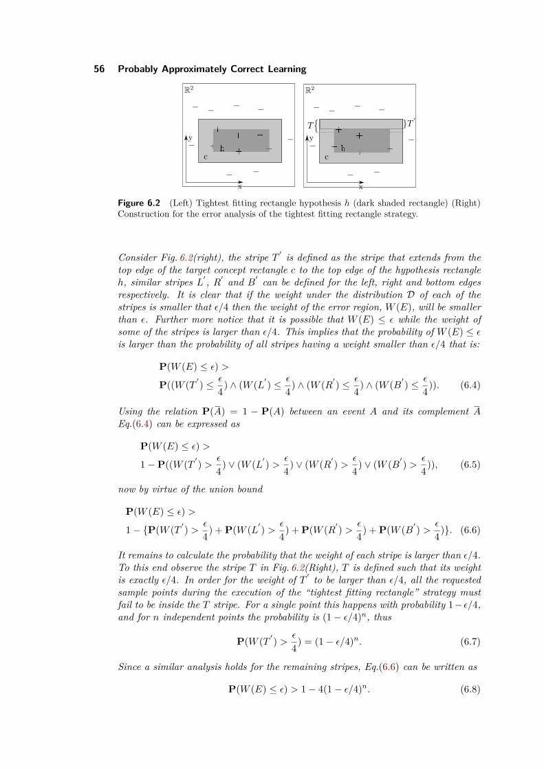
56 Probably Approximately Correct Learning
Figure 6.2 (Left) Tightest fitting rectangle hypothesis h (dark shaded rectangle) (Right)Construction for the error analysis of the tightest fitting rectangle strategy.
Consider Fig. 6.2(right), the stripe T ′ is defined as the stripe that extends from thetop edge of the target concept rectangle c to the top edge of the hypothesis rectangleh, similar stripes L′, R′ and B′ can be defined for the left, right and bottom edgesrespectively. It is clear that if the weight under the distribution D of each of thestripes is smaller that ε/4 then the weight of the error region, W (E), will be smallerthan ε. Further more notice that it is possible that W (E) ≤ ε while the weight ofsome of the stripes is larger than ε/4. This implies that the probability of W (E) ≤ εis larger than the probability of all stripes having a weight smaller than ε/4 that is:
P(W (E) ≤ ε) >
P((W (T ′) ≤ ε
4) ∧ (W (L′) ≤ ε
4) ∧ (W (R′) ≤ ε
4) ∧ (W (B′) ≤ ε
4)). (6.4)
Using the relation P(A) = 1 − P(A) between an event A and its complement AEq.(6.4) can be expressed as
P(W (E) ≤ ε) >
1−P((W (T ′) > ε
4) ∨ (W (L′) > ε
4) ∨ (W (R′) > ε
4) ∨ (W (B′) > ε
4)), (6.5)
now by virtue of the union bound
P(W (E) ≤ ε) >
1− P(W (T ′) > ε
4) + P(W (L′) > ε
4) + P(W (R′) > ε
4) + P(W (B′) > ε
4). (6.6)
It remains to calculate the probability that the weight of each stripe is larger than ε/4.To this end observe the stripe T in Fig. 6.2(Right), T is defined such that its weightis exactly ε/4. In order for the weight of T ′ to be larger than ε/4, all the requestedsample points during the execution of the “tightest fitting rectangle” strategy mustfail to be inside the T stripe. For a single point this happens with probability 1− ε/4,and for n independent points the probability is (1− ε/4)n, thus
P(W (T ′) > ε
4) = (1− ε/4)n. (6.7)
Since a similar analysis holds for the remaining stripes, Eq.(6.6) can be written as
P(W (E) ≤ ε) > 1− 4(1− ε/4)n. (6.8)
6.0 Probably Approximately Correct Learning 57
Finally if n is chosen such that 4(1 − ε/4)n ≤ δ then with probability at least 1 − δthe strategy will yield a hypothesis rectangle h with error at most ε. Furthermore therectangles are efficiently PAC learnable: using the inequality (1−x) ≤ e−x it followsthat
4(1− ε/4)n ≤ 4e−nε4 ≤ δ, (6.9)
observe that if n is such that the second inequality holds, so does the first one.Therefore if n ≥ 4
ε ln(4δ ) then Eq.(6.9) is satisfied.

58 Probably Approximately Correct Learning

Chapter 7
Final note
This script contains and introduction to all but one of the topics discussed in theSLT course, the Vapnik–Chervonenkis theory. This subject is to be included infuture versions of the script, in the mean time the interested reader is encouragedto explore chapter 12 of the text by ? as well as ?. The reader is also encouragedto go through the provided references (original research papers and books) wheremore in depth details of the covered topics can be found.

60 Final note
Chapter A
Notions of probability
Before introducing the main questions of statistical learning theory such as: howcan the quality of a classifier be measured? What guarantees are there for errorprediction? Or the main methods and techniques of the field like maximum entropyprinciple, deterministic annealing, graph based clustering and reinforcement learn-ing among others, some notions of probability theory are required. The conceptsand definitions that follow can be found in the book “Probability” by ?.
Definition 9 (Sample point and Sample space). Consider an experiment with a finitenumber N of possible outcomes ωi, i = 1, 2, . . . , N . For instance dice tossing or urnsand ballots drawing experiments. The ωi will be called sample points or elementaryevents and the set Ω = ω1, ω2, . . . , ωn will be denoted as sample space.
Example 6 (n coin flips). Assume a coin is tossed n times, if 0, 1 are used todesignate head and tail respectively, a sample point ω will be a sequence of the form(a1, a2, . . . , an) ai ∈ 0, 1 and the sample space will be the set Ω = ω : ω =(a1, a2, . . . , an) ai ∈ 0, 1. Notice that the cardinality of Ω (number of elements)is N(Ω) = 2n
Once the ideas of sample points and sample space are defined, it is possible tointroduce the concepts of events and event algebra as follows:
Definition 10 (Events). Let Ω be a sample space and A ⊂ Ω. If under the constrainsof the experiment that defines Ω, it is possible to assert ω ∈ A or ω /∈ A for everyoutcome ω, then A is an event.
62 Notions of probability
Definition 11 (Event algebra). Let A be a collection of subsets of Ω. If the conditions
• Ω ∈ A
• A ∈ A, B ∈ A implies that A ∪B,A ∩B and A \B belong to A
holds then A is said to be an event algebra
Example 7 (Event algebras). Let Ω be a sample space, the following are examples ofevent algebras
• A = Ω, ∅ (Trivial algebra)
• A = P(Ω) = A : A ⊆ Ω (Power set algebra)
• A = A,A,Ω, ∅ where A is an event and A = Ω \ A is its complementaryevent
• All sequences of of n coin flips with n2 (1 + ε) heads or more
In order to define a probabilistic model of an experiment is not enough to set thesample points, sample space and event algebra it is also required to assign to everysample point ωi ∈ Ω a weight pi = p(ωi), referred as probability of the outcome i,with the properties
• 0 ≤ pi ≤ 1 (non-negativity)
•∑i pi = 1 (Normalization).
Once the probabilities of the sample points are given, the probability of an event isdefined as
Definition 12 (Event probability). Let A be an element of an event algebra A. Theprobability P(A) of an event A is given by
P(A) =∑
i:ωi∈Api .
Observe that the following properties of event probabilities follow from the defi-nition
• P(Ω) = 1
• P(A ∪B) = P(A) + P(B)−P(A ∩B)
• P(A) = 1−P(A)
Finally a probability model is a triplet (Ω,A, P ) where Ω is a sample space, A is anevent algebra and P = P(A) : A ∈ A is a probability measure. Given a proba-bilistic model of an experiment, the interest is not only on the possible outcomes butalso on numerical properties that depend on the outcome of the experiment, that ison quantities that can be measured. To formalize this idea the concept of randomvariable is introduced as follows:
A.0 Notions of probability 63
Definition 13 (Random variable (simple)). Any numerical function ξ : Ω → R de-fined on a finite sample space Ω, is called a random variable.
Example 8 (Indicator function). Let (Ω,A,P) be a probability model the indicatoror characteristic function of the set A ∈ A is given by
IA(ω) =
1 if ω ∈ A0 if ω /∈ A
Consider now a probability model (Ω,A,P) and a random variable ξ, as alreadynoted most of the time the focus is not directly on the outcomes ωi but rather ratherin the values xi that the random variable can take. Since Ω is finite so is the setX = x1, . . . , xm of possible values of ξ. If X is taken as a sample space and P(X)as an event algebra then ξ induces a probability on (X,P(X)) given by
Pξ(B) = Pω : ξ(ω) ∈ B, B ∈ P(X), (A.1)
definition 12 implies thatPξ(B) =
∑i:xi∈B
pξ(xi), (A.2)
thus the value of Pξ(B) is determined by
pξ(xi) = Pω : ξ(ω) = xi (A.3)
Definition 14 (Probability of a random variable). The set pξ(x1), . . . , pξ(xm) iscalled the probability distribution of the random variable ξ
An equivalent description of the probability structure of a random variable canbe given by the Distribution function
Definition 15 (Distribution function). Let x ∈ R. The function
Fξ(x) = Pω : ξ(ω) ≤ x
is called distribution function of the random variable ξ
Observe that the distribution function of random variable ξ can also be writtenas
Fξ(x) =∑i:xi≤x
Pξ(xi).
Let (Ω,A,P) be a finite probability model, ξ(ω) a random variable with values inthe set X = x1, . . . , xm, and define the family of pairwise disjoint sets Ai = ω :ξ(ω) = xi. It follows that ξ can be represented as
ξ(ω) =m∑i=1
xiIAi(ω),
where the indicator function IAi was defined in Example 8
Definition 16 (Expectation value). The expectation value of a random variable ξ isthe number defined by
Eξ =m∑i=1
xiP(Ai) =∑i
xiPξ(xi)