Embed Size (px)
Citation preview

Statistical InferenceStatistical InferenceJune 30-July 1, 2004June 30-July 1, 2004

Statistical InferenceStatistical Inference The process of making The process of making
guesses about the truth from a guesses about the truth from a sample. sample.
Sample (observation)
Make guesses about the whole population
Truth (not observable)

FOR EXAMPLE: What’s the average weight of all medical students in the US?
1. We could go out and measure all US medical students (>65,000)
2. Or, we could take a sample and make inferences about the truth from our sample.
Using what we observe,
1. We can test an a priori guess (hypothesis testing).
2. We can estimate the true value (confidence intervals).

Statistical Inference is based Statistical Inference is based on Sampling Variabilityon Sampling Variability
Sample Statistic – we summarize a sample into one number; e.g., could be a mean, a difference in means or proportions, or an odds ratio – E.g.: average blood pressure of a sample of 50 American men– E.g.: the difference in average blood pressure between a sample of 50
men and a sample of 50 women
Sampling Variability – If we could repeat an experiment many, many times on different samples with the same number of subjects, the resultant sample statistic would not always be the same (because of chance!).
Standard Error – a measure of the sampling variability (a function of sample size).

Sampling VariabilitySampling Variability
Random students
The Truth (not knowable)
The average of all 65,000+ US medical students at this moment is exactly 150 lbs
175.9 lbs
189.3 lbs
92.1 lbs
152.3 lbs
169.2 lbs
110.3 lbs

Sampling VariabilitySampling VariabilityRandom samples of 5 students
The Truth (not knowable)
The average of all 65,000+ US medical students at this moment is exactly 150 lbs
135.9 lbs
139.3 lbs
152.1 lbs
158.3 lbs
149.2 lbs
170.3 lbs
Sampling VariabilitySampling Variability
Samples of 50 students
The Truth (not knowable)
The average of all 65,000+ US medical students at this moment is exactly 150 lbs
146.9 lbs
148.9 lbs
150.0 lbs
152.3 lbs
147.2 lbs
155.3 lbs

Sampling VariabilitySampling Variability
Samples of 150 students
The Truth (not knowable)
The average of all 65,000+ US medical students at this moment is exactly 150 lbs
150.31 lbs
150.02 lbs
149.8 lbs
149.95 lbs
150.3 lbs
150.9 lbs

The Central Limit Theorem: The Central Limit Theorem: how sample statistics varyhow sample statistics vary
Many sample statistics (e.g., the sample average) follow a normal distribution – centers around the true population value (e.g. the true
mean weight) – Becomes less variable (by a predictable amount) as
sample size increases: Standard error of a sample statistic = standard deviation /
square root (sample size) Remember: standard deviation reflects the average variability
of the characteristic in the population

The Central Limit Theorem:The Central Limit Theorem:IllustrationIllustration
I had SAS generate 1000 random observations from the following probability distributions:
~N(10,5)~Exp(1)Uniform on [0,1]~Bin(40, .05)

~N(10,5)~N(10,5)

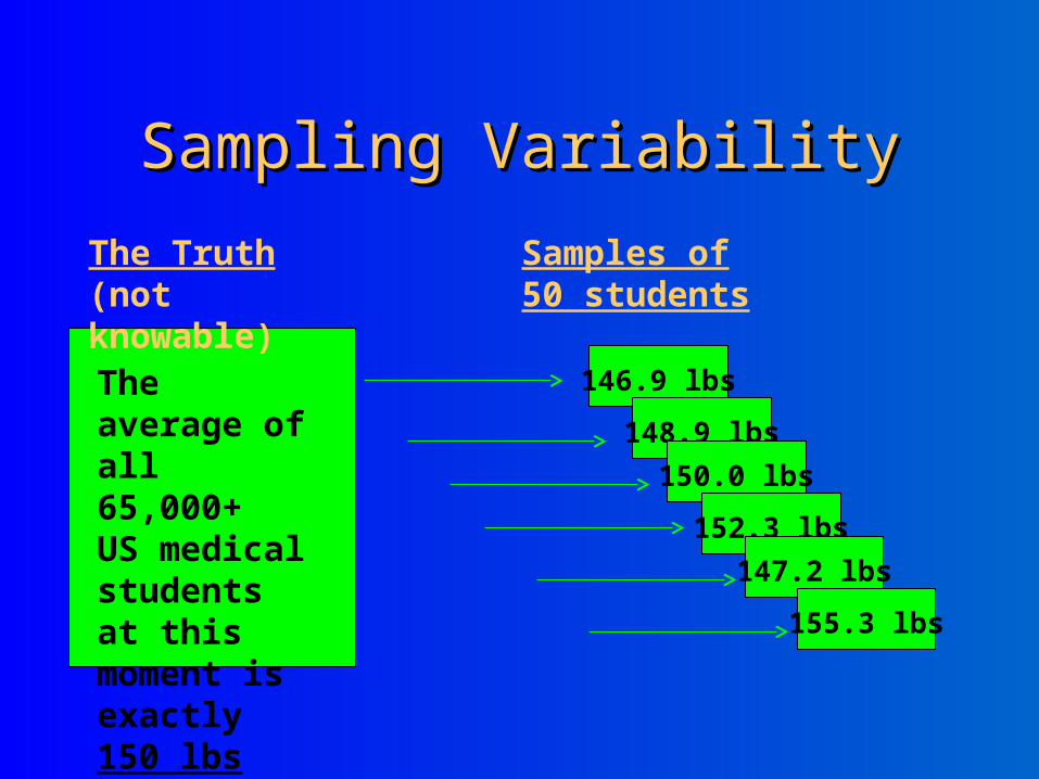
Uniform on [0,1]Uniform on [0,1]

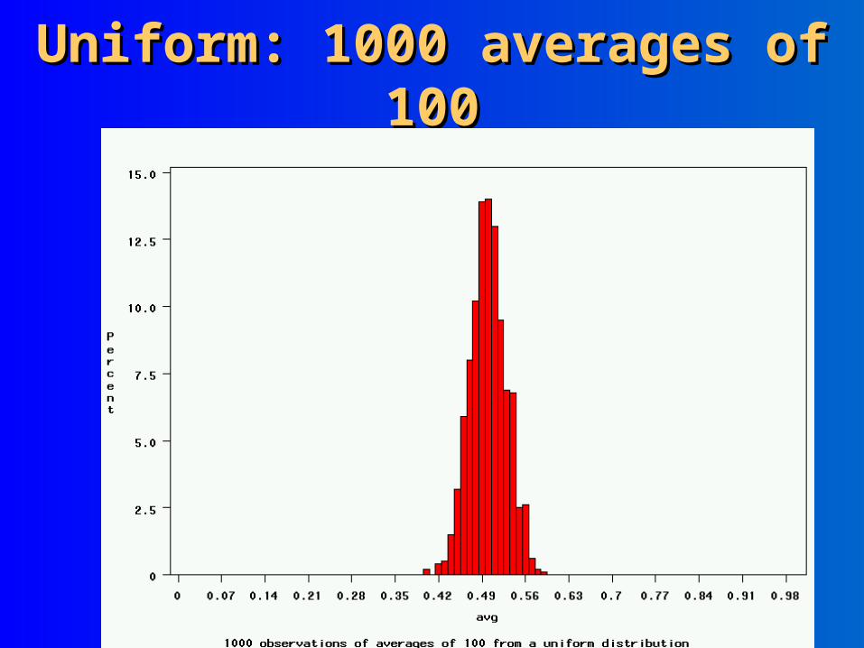
~Exp(1)~Exp(1)

~Bin(40, .05)~Bin(40, .05)

The Central Limit Theorem:The Central Limit Theorem:IllustrationIllustration
I then had SAS generate averages of 2, averages of 5, and averages of 100 random observations from each probability distributions…
(Refer to end of SAS LAB ONE, which we will implement next Wednesday, July 7)

~N(10,25): average of 1~N(10,25): average of 1(original distribution)(original distribution)

~N(10,25): 1000 averages of 2~N(10,25): 1000 averages of 2

~N(10,25): 1000 averages of 5~N(10,25): 1000 averages of 5

~N(10,25): 1000 averages of 100~N(10,25): 1000 averages of 100

Uniform on [0,1]: average of 1Uniform on [0,1]: average of 1(original distribution)(original distribution)

Uniform: 1000 averages of 2Uniform: 1000 averages of 2

Uniform: 1000 averages of 5Uniform: 1000 averages of 5
Uniform: 1000 averages of 100Uniform: 1000 averages of 100

~Exp(1): average of 1~Exp(1): average of 1(original distribution)(original distribution)
~Exp(1): 1000 averages of 2~Exp(1): 1000 averages of 2

~Exp(1): 1000 averages of 5~Exp(1): 1000 averages of 5

~Exp(1): 1000 averages of 100~Exp(1): 1000 averages of 100

~Bin(40, .05): average of 1~Bin(40, .05): average of 1(original distribution)(original distribution)

~Bin(40, .05): 1000 averages of 2~Bin(40, .05): 1000 averages of 2
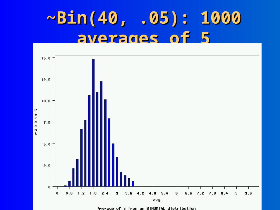
~Bin(40, .05): 1000 averages of 5~Bin(40, .05): 1000 averages of 5

~Bin(40, .05): 1000 averages of 100~Bin(40, .05): 1000 averages of 100

The Central Limit Theorem: The Central Limit Theorem: formallyformally
If all possible random samples, each of size n, are taken from any population with a mean and a standard deviation , the sampling distribution of the sample means (averages) will:
x1. have mean:
nx
2. have standard deviation:
3. be approximately normally distributed regardless of the shape of the parent population (normality improves with larger n)

Example Example
Pretend that the mean weight of medical students was 128 lbs with a
standard deviation of 15 lbs…

Hypothetical histogram of Hypothetical histogram of weights of US medical students weights of US medical students
(computer-generated) (computer-generated)
69 77 85 93 101 109 117 125 133 141 149 157 165 173 181 189 197
0
0.5
1.0
1.5
2.0
2.5
3.0
P e r c e n t
Weight in pounds
mean= 128 lbs; standard deviation = 15 lbs
Standard deviation reflects the natural variability of weights in the population

80 87 94 101 108 115 122 129 136 143 150 157 164 171 178 185 192 199
0
0.5
1.0
1.5
2.0
2.5
3.0
3.5
4.0
P e r c e n t
The average weight of a pair of students
Average weights from 1000 Average weights from 1000 samples of 2samples of 2
lbs6.102
15 mean theoferror standard

Average weights from 1000 Average weights from 1000 samples of 10samples of 10
80 87 94 101 108 115 122 129 136 143 150 157 164 171 178 185 192 199
0
1
2
3
4
5
6
7
8
9
P e r c e n t
The average weight of 10 students
lbs74.410
15 mean theoferror standard
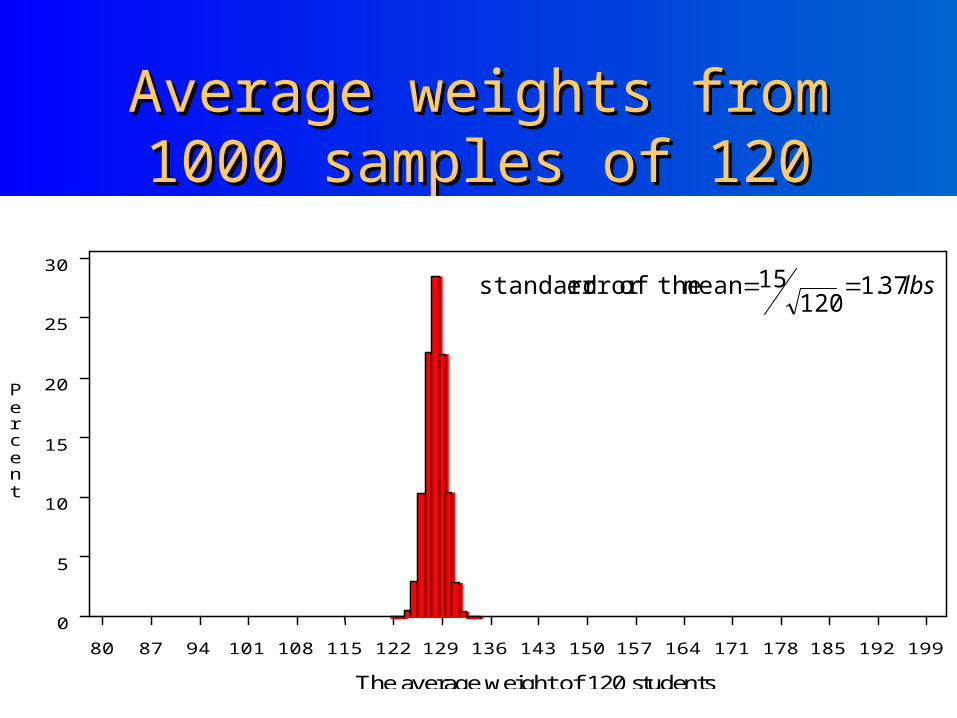
Average weights from 1000 Average weights from 1000 samples of 120samples of 120
80 87 94 101 108 115 122 129 136 143 150 157 164 171 178 185 192 199
0
5
10
15
20
25
30
P e r c e n t
The average weight of 120 students
lbs37.1120
15 mean theoferror standard

Using Sampling VariabilityUsing Sampling Variability
In reality, we only get to take one sample!!
But, since we have an idea about how sampling variability works, we can make inferences about the truth based on one sample.

Hypothesis TestingHypothesis Testing

Hypothesis TestingHypothesis Testing
The null hypothesis is the “straw man” that we are trying to shoot down.
Example 1: Possible null hypothesis: “mean weight of medical students = 128 lbs”
Let’s say we take one sample of 120 medical students and calculate their average weight….

Expected Sampling Variability for n=120 Expected Sampling Variability for n=120 ifif the true weight is 128 (and SD=15) the true weight is 128 (and SD=15)
80 87 94 101 108 115 122 129 136 143 150 157 164 171 178 185 192 199
0
5
10
15
20
25
30
P e r c e n t
The average weight of 120 students
What are we going to think if our 120-student sample has an average weight of 143??

““P-value” associated with this experimentP-value” associated with this experiment
80 87 94 101 108 115 122 129 136 143 150 157 164 171 178 185 192 199
0
5
10
15
20
25
30
P e r c e n t
The average weight of 120 students
“P-value” (the probability of our sample average being 143 lbs or more IF the true average weight is
128) < .0001
Gives us evidence that 128 isn’t a good guess

Estimation (a preview)Estimation (a preview)
80 87 94 101 108 115 122 129 136 143 150 157 164 171 178 185 192 199
0
5
10
15
20
25
30
P e r c e n t
The average weight of 120 students
We’d estimate based on these data that the average weight is somewhere closer to 143 lbs. And we could state the precision of this estimate (a “confidence interval”—to come later)

80 87 94 101 108 115 122 129 136 143 150 157 164 171 178 185 192 199
0
0.5
1.0
1.5
2.0
2.5
3.0
3.5
4.0
P e r c e n t
The average weight of a pair of students
Expected Sampling Variability for n=2Expected Sampling Variability for n=2
What are we going to think if our 2-student sample has an average weight of 143?

80 87 94 101 108 115 122 129 136 143 150 157 164 171 178 185 192 199
0
0.5
1.0
1.5
2.0
2.5
3.0
3.5
4.0
P e r c e n t
The average weight of a pair of students
P-value = 11%
i.e. about 11 out of 100 “average of 2” experiments will yield values 143 or higher even if the true mean weight is only 128
Expected Sampling Variability for n=2Expected Sampling Variability for n=2

The P-valueThe P-value
P-value is the probability that we would have seen our data (or something more unexpected) just by chance if the null hypothesis (null value) is true.
Small p-values mean the null value is unlikely given our data.

The P-valueThe P-value
By convention, p-values of <.05 are often accepted as “statistically significant” in the medical literature; but this is an arbitrary cut-off.
A cut-off of p<.05 means that in about 5 of 100 experiments, a result would appear significant just by chance (“Type I error”).

What factors affect the p-What factors affect the p-value?value?
The effect sizeVariability of the sample data
Sample size**

Statistical PowerStatistical Power
Note that, though we found the same sample value (143 lbs) in our 120-student sample and our 2-student sample, we only rejected the null (and concluded that med students weigh more on average than 128 lbs) based on the 120-student sample.
Larger samples give us more statistical power…

Hypothesis Testing: example 2Hypothesis Testing: example 2
Hypothesis: more babies born in November (9 months after Valentine’s Day)
Empirical evidence: Our researcher observed that 6/19 kids in one classroom had November birthdays.

Hypothesis TestingHypothesis Testing
Is a contest between…
The Null Hypothesis and the Alternative Hypothesis– The null hypothesis (abbreviated H0) is usually the
hypothesis of no difference Example: There are no more babies born in November (9
months after Valentine’s Day) than any other month
– The alternative hypothesis (abbreviated Ha) Example: There are more babies born in November (9 months
after Valentine’s Day) than in other months

The StepsThe Steps1. Define your null and alternative hypotheses:
– H0: P(being born in November)=1/12
– Ha: P(being born in November)>1/12
“one-sided” test

The StepsThe Steps 2. Figure out the “null distribution”:
– If I observe a class of 19 students and each student has a probability of 1/12 th of being born in November…
– Sounds BINOMIAL!– In MATH-SPEAK: Class ~ binomial (19, 1/12th)
***If the null is true, how many births should I expect to see? – Expected November births= 19*(1/12)= 1.5 why?– Reasonable Variability = [19*(1/12)*(11/12)]**1/2 = 1.2 why?If I see 0-3 November births, it seems reasonable that the null is
true…anything else is suspicious…

The StepsThe Steps3. Observe (experimental data)
We see 6/19 babies were born in November in this case.

The StepsThe Steps
4. Calculate a “p-value” and compare to a preset “significance level”

The Almighty P-ValueThe Almighty P-Value
The P-value roughly translated is… “the probability of seeing something as extreme as you did due to chance alone”
Example: The probability that we would have seen 6 or more November births out of 19 if the probability of a random child being born in November was only 1/12.
Easy to Calculate in SAS:
data _null_;
pval = 1- CDF('BINOMIAL',5, (1/12), 19);
put pval;
run;
0.003502582
Based on the null distribution

The StepsThe Steps
4a. Calculate a “p-value”
data _null_;
pval = 1- CDF('BINOMIAL',5, (1/12), 19);
put pval;
run;
0.003502582
b. and compare to a preset “significance level”….
.0035<.05
5% is often chosen due to convention/history
The StepsThe Steps
5. Reject or fail to reject (accept) Ho.
In this case, reject Ho.

Summary: The Underlying Summary: The Underlying Logic…Logic…
Follows this logic:
Assume A.
If A, then B.
Not B.
Therefore, Not A.
But throw in a bit of uncertainty…If A, then probably B…

Summary: It goes something Summary: It goes something like this…like this…
The assumption: The probability of being born in November is 1/12th.
If the assumption is true, then it is highly likely that we will see fewer than 6 November-births (since the probability of seeing 6 or more is .0035, or 3-4 times out of 1000).
We saw 6 November-births. Therefore, the assumption is likely to be wrong.

Example 3: the odds ratioExample 3: the odds ratio
Null hypothesis: There is no association between an exposure and a disease (odds ratio=1.0).

0.3 1.0 2.0 3.0 0
1
2
3
4
5
6
P e r c e n t
Observed Odds Ratio
Example 3: Sampling Variability of the null Odds Ratio (OR) (100 cases/100 controls/10% exposed)

The Sampling Variability of the natural log of the OR (lnOR) is more Gaussian
0 0
2
4
6
8
10
P e r c e n t
lnOR
Sample values far from lnOR=0 give us evidence of an association. These values are very unlikely if there’s no association in nature.

Statistical PowerStatistical Power
Statistical power here is the probability of concluding that there is an association between exposure and disease if an association truly exists.– The stronger the association, the more likely we are to
pick it up in our study.– The more people we sample, the more likely we are to
conclude that there is an association if one exists (because the sampling variability is reduced).

Error and PowerError and Power
Type-I Error (false positive): – Concluding that the observed effect is real when it’s
just due to chance.
Type-II Error (false negative):
– Missing a real effect.
POWER (the flip side of type-II error):
– The probability of seeing a real effect.

Your Decision
The TRUTH
God Exists God Doesn’t Exist
Reject GodBIG MISTAKE Correct
Accept God Correct—Big Pay Off
MINOR MISTAKE
Think of…Think of…
Pascal’s WagerPascal’s Wager

Type I and Type II Error in a boxType I and Type II Error in a box
Your Statistical Decision
True state of null hypothesis (H0)
H0 True H0 False
Reject H0 Type I error (α) Correct
Do not reject H0
Correct Type II Error (β)

Statistical vs. Clinical Statistical vs. Clinical SignificanceSignificance
Consider a hypothetical trial comparing death rates in 12,000 patients with multi-organ failure receiving a new inotrope, with 12,000 patients receiving usual care.
If there was a 1% reduction in mortality in the treatment group (49% deaths versus 50% in the usual care group) this would be statistically significant (p<.05), because of the large sample size.
However, such a small difference in death rates may not be clinically important.

Confidence Intervals Confidence Intervals (Estimation)(Estimation)

Confidence Intervals Confidence Intervals (Estimation)(Estimation)
Confidence intervals don’t presuppose a null value.
Shows our best guess at the plausible range of values for the population characteristic based on our data.
The 95% confidence interval contains the true population value approximately 95% of the time.

95% CI should contain true 95% CI should contain true value ~ 19/20 timesvalue ~ 19/20 times
X = TRUE VALUE
(--------------------X-----------------)
(-------- X-------------------------)
(---------------------X----------------)
X (-----------------------------------)
(-----------------X----------------)
(----------------------X----------------)
(----X---------------------------------)

Confidence IntervalsConfidence Intervals
(Sample statistic) (measure of how confident we want to be) (standard error)

95% CI from a sample of 120:95% CI from a sample of 120:143 +/- 2 143 +/- 2 x x (1.37) = 140.26 --145.74(1.37) = 140.26 --145.74
80 87 94 101 108 115 122 129 136 143 150 157 164 171 178 185 192 199
0
5
10
15
20
25
30
P e r c e n t
The average weight of 120 students
lbs37.1120
15 mean theoferror standard

95% CI from a sample of 10:95% CI from a sample of 10:143 +/- 2 143 +/- 2 x x (4.74) = 133.52 –152.48(4.74) = 133.52 –152.48
80 87 94 101 108 115 122 129 136 143 150 157 164 171 178 185 192 199
0
1
2
3
4
5
6
7
8
9
P e r c e n t
The average weight of 10 students
lbs74.410
15 mean theoferror standard

99.7% CI from a sample of 10:99.7% CI from a sample of 10:143 +/- 3 143 +/- 3 x x (4.74) = 128.78 –157.22(4.74) = 128.78 –157.22
80 87 94 101 108 115 122 129 136 143 150 157 164 171 178 185 192 199
0
1
2
3
4
5
6
7
8
9
P e r c e n t
The average weight of 10 students
lbs74.410
15 mean theoferror standard

What Confidence Intervals doWhat Confidence Intervals do
They indicate the un/certainty about the size of a population characteristic or effect. Wider CI’s indicate less certainty.
Confidence intervals can also answer the question of whether or not an association exists or a treatment is beneficial or harmful. (analogous to p-values…)
e.g., if the CI of an odds ratio includes the value 1.0 we cannot be confident that exposure is associated with disease.