Chapter 6: Statistical Inference (Single Sample)

Shiwen Shen

University of South Carolina

2017 Summer

1 / 56

Introduction

I Statistical inference can be classified as estimation problem andtesting problem.

I The goal of estimation is to make a proper guess of unknownparameter, e.g. population mean µ, population proportion p, etc,using data.

I The goal of testing is to exam whether the estimated value for theunknown parameter is good, or whether some statistical argument iscorrect.

I In this chapter, we discuss the estimation and testing methods basedon single sample, forcusing on population proportion and populationmean.

2 / 56

Inference on Population Proportion

The population proportion p emerges when the characteristic wemeasure on each individual is categorical, or simply binary (i.e., only2 outcomes possible). Here are some examples:

p = proportion of airline has experienced exceedance

p = proportion of defective water filters in a factory

p = proportion of HIV positive in SC

We can connect these binary outcomes to the Bernoulli trailsassumptions for each individual in the sample:

1. Each trial results in only two possible outcomes, labeled as“success” and “failure.”

2. The trials are independent.

3. The probability of a success in each trial, denoted as p, remainsconstant. It follows that the probability of a failure in each trialis 1− p.

3 / 56

Point Estimator of Proportion p

I Suppose we define Y = the number of successes out of nsampled individuals so Y ∼ b(n, p). A natural point estimatorfor p, the population proportion, is

p̂ =Y

n,

the sample proportion. p̂ is read as p hat.

4 / 56

Property of p̂

I p̂ is a unbiased estimator of p. That is,

E (p̂) = p.

I To quantify the precision of p̂,

var(p̂) =p(1− p)

n

I Question: What is the (asymptotic) distribution of p̂?

5 / 56

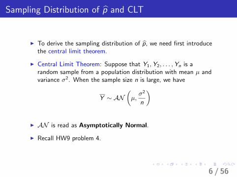
Sampling Distribution of p̂ and CLT

I To derive the sampling distribution of p̂, we need first introducethe central limit theorem.

I Central Limit Theorem: Suppose that Y1,Y2, . . . ,Yn is arandom sample from a population distribution with mean µ andvariance σ2. When the sample size n is large, we have

Y ∼ AN(µ,σ2

n

)

I AN is read as Asymptotically Normal.

I Recall HW9 problem 4.

6 / 56

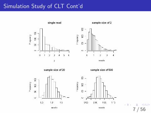
Simulation Study of CLT Cont’d

7 / 56

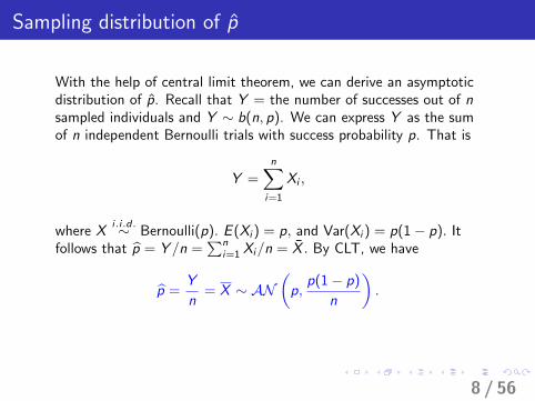
Sampling distribution of p̂

With the help of central limit theorem, we can derive an asymptoticdistribution of p̂. Recall that Y = the number of successes out of nsampled individuals and Y ∼ b(n, p). We can express Y as the sumof n independent Bernoulli trials with success probability p. That is

Y =n∑

i=1

Xi ,

where Xi.i.d.∼ Bernoulli(p). E (Xi ) = p, and Var(Xi ) = p(1− p). It

follows that p̂ = Y /n =∑n

i=1 Xi/n = X̄ . By CLT, we have

p̂ =Y

n= X ∼ AN

(p,

p(1− p)

n

).

8 / 56

Confidence Interval

I Using a point estimator only ignores important information;namely, how variable the estimator is.

I To avoid this problem (i.e., to account for the uncertainty in thesampling procedure), we therefore pursue the topic of intervalestimation (also known as confidence intervals).

I The main difference between a point estimate and an intervalestimate is that

I a point estimate is a one-shot guess at the value of theparameter; this ignores the variability in the estimate.

I an interval estimate (i.e., confidence interval) is an interval ofvalues. It is formed by taking the point estimate and thenadjusting it downwards and upwards to account for the pointestimate’s variability.

9 / 56

Confidence Interval for p

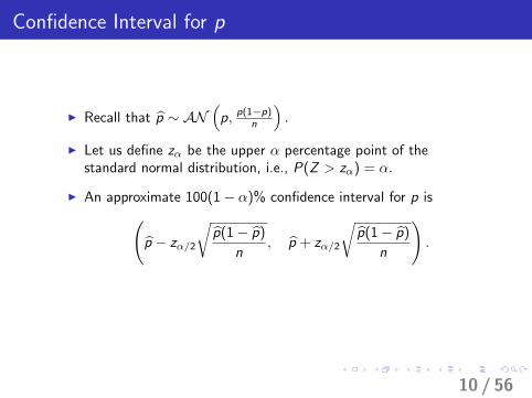
I Recall that p̂ ∼ AN(p, p(1−p)

n

).

I Let us define zα be the upper α percentage point of thestandard normal distribution, i.e., P(Z > zα) = α.

I An approximate 100(1− α)% confidence interval for p is(p̂ − zα/2

√p̂(1− p̂)

n, p̂ + zα/2

√p̂(1− p̂)

n

).

10 / 56

Confidence Interval for p cont’d

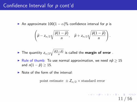
I An approximate 100(1− α)% confidence interval for p is(p̂ − zα/2

√p̂(1− p̂)

n, p̂ + zα/2

√p̂(1− p̂)

n

).

I The quantity zα/2

√p̂(1−p̂)

n is called the margin of error .

I Rule of thumb: To use normal approximation, we need np̂ ≥ 15and n(1− p̂) ≥ 15.

I Note of the form of the interval:

point estimate ± Zα/2 × standard error

11 / 56

Interpretation of Confidence Interval

I Suppose that we are interested in parameter p for certainpopulation. We take a sample of size n and calculate the sampleproportion p̂ = Y /n. A 95% confidence interval is given by

Point. Est± 1.96 Standard Error.

I The 95% confidence comes from the fact that if we repeatedthis experiment over and over again, apprxomiately, 95% of allsamples would produce a confidence interval that contains thetrue proportion, and only 5% of the time would the interval bein error.

I We call 100(1− α)% the confidence level.

12 / 56

Interpretation of Confidence Interval Cont’d

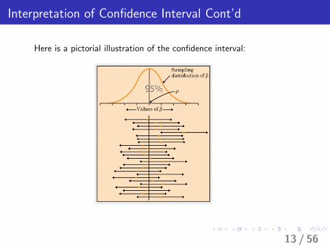
Here is a pictorial illustration of the confidence interval:

13 / 56

Statistical Hypothesis

I Definition: a statistical hypothesis is an assertion or conjectureconcerning one or more population parameters.

I Example:

1. The proportion of underweight milk is more then 3% in a localfarm.

2. More than 7% of the landings for a certain airline exceed therunway.

3. The defective rate of the water filter is less than 5%.

14 / 56

4 Steps to a Hypothesis Test

1. State the null (H0) and alternative (Ha or H1) hypotheses.

2. Collect the data and calculate test statistic assuming H0 istrue.

3. Assuming the H0 is true, calculate the p-value.

4. Draw conclusion based on the p-value. We either reject H0 orfail to reject H0.

Let us look at an example to illustrate these steps...

15 / 56

Example: Defective Water Filters

I Historically, the defective rate of water filters is 7% in a certainfactory. A new quality control system is introduced to reducethe defective rate. Suppose that we randomly choose 300 waterfilters, and calculate p̂ = 0.041. We want to test whether thenew system reduce the defective rate or not.

I Let p=proportion of defective water filters in the factory afterintroducing the new system.

16 / 56

Step 1: The Null and Alternative Hypothesis

I Null hypothesis is denoted by H0, which represents what weassume to be true. Under null hypothesis, the exact value of theparameter is specified.

I Alternative hypothesis is denoted by Ha or H1, which representsthe researcher’s interest.

I In most situation, researchers want to reject null hypothesis infavor of the alternative hypothesis by performing someexperiment.

I In defective water filters example,

H0 : p = 0.07

Ha : p < 0.07 (the new system reduces the defective rate)

17 / 56

Step 2: Calculate test statistic

I How should we make our decision based on the sample?

I We reject H0, if p̂ is far less than 0.07, which is not likely tohappen if assuming p = 0.07.

I We need the sampling distribution to quantify how far is far.

18 / 56

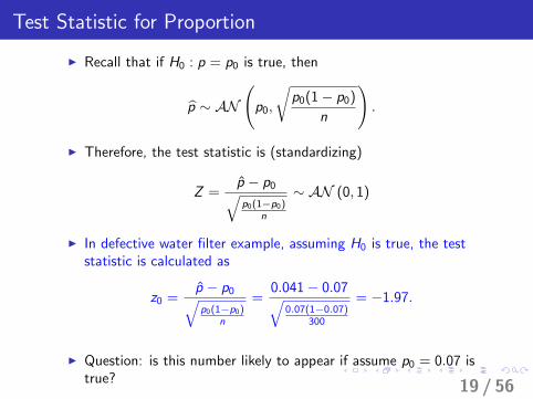
Test Statistic for Proportion

I Recall that if H0 : p = p0 is true, then

p̂ ∼ AN

(p0,

√p0(1− p0)

n

).

I Therefore, the test statistic is (standardizing)

Z =p̂ − p0√p0(1−p0)

n

∼ AN (0, 1)

I In defective water filter example, assuming H0 is true, the teststatistic is calculated as

z0 =p̂ − p0√p0(1−p0)

n

=0.041− 0.07√

0.07(1−0.07)300

= −1.97.

I Question: is this number likely to appear if assume p0 = 0.07 istrue? 19 / 56

Step 3: Calculate p-value

I The p-value is the probability of getting the sample results yougot or something more extreme assuming that the nullhypothesis is true.

I If the p-value is small, we doubt the null hypothesis since it isnot likely to observe such a ”extreme” test statistic under H0.There is evidence to against null hypothesis.

I On the other hand, if the p-value is large, we have a pretty goodchance to observe the computed test statistic under H0 in asingle experiment, there is no reason to question the H0.

I In other words, the p-value for a hypothesis test measures howmuch evidence we have against H0, that is,

the smaller the p-value =⇒ the more evidence against H0

20 / 56

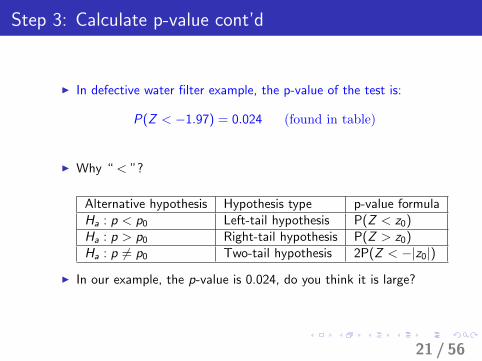
Step 3: Calculate p-value cont’d

I In defective water filter example, the p-value of the test is:

P(Z < −1.97) = 0.024 (found in table)

I Why “ < ”?

Alternative hypothesis Hypothesis type p-value formulaHa : p < p0 Left-tail hypothesis P(Z < z0)Ha : p > p0 Right-tail hypothesis P(Z > z0)Ha : p 6= p0 Two-tail hypothesis 2P(Z < −|z0|)

I In our example, the p-value is 0.024, do you think it is large?

21 / 56

Step 4: Conclusion

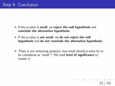
I If the p-value is small, we reject the null hypothesis andconclude the alternative hypothesis.

I If the p-value is not small, we do not reject the nullhypothesis and do not conclude the alternative hypothesis.

I There is one remaining question, how small should p-value be tobe considered as ”small”? We need level of significance toanswer it.

22 / 56

Step 4: Conclusion cont’d

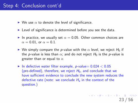
I We use α to denote the level of significance.

I Level of significance is determined before you see the data.

I In practice, we usually set α = 0.05. Other common choices areα = 0.01, or α = 0.1.

I We simply compare the p-value with the α level, we reject H0 ifthe p-value is less than α; and do not reject H0 is the p-value isgreater than or equal to α

I In defective water filter example, p-value= 0.024 < 0.05(pre-defined), therefore, we reject H0, and conclude that wehave sufficient evidence to conclude the new system reduces thedefective rate (note: we conclude Ha in the context of thequestion.)

23 / 56

Example: Exceedance of the Localizer

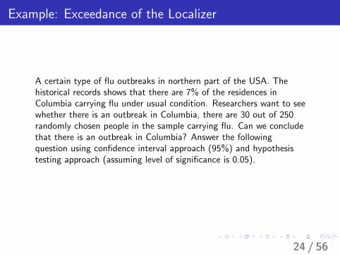
A certain type of flu outbreaks in northern part of the USA. Thehistorical records shows that there are 7% of the residences inColumbia carrying flu under usual condition. Researchers want to seewhether there is an outbreak in Columbia, there are 30 out of 250randomly chosen people in the sample carrying flu. Can we concludethat there is an outbreak in Columbia? Answer the followingquestion using confidence interval approach (95%) and hypothesistesting approach (assuming level of significance is 0.05).

24 / 56

Inference for p: Confidence Interval Approach

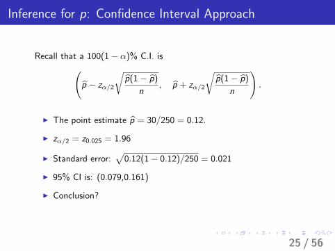
Recall that a 100(1− α)% C.I. is(p̂ − zα/2

√p̂(1− p̂)

n, p̂ + zα/2

√p̂(1− p̂)

n

).

I The point estimate p̂ = 30/250 = 0.12.

I zα/2 = z0.025 = 1.96

I Standard error:√

0.12(1− 0.12)/250 = 0.021

I 95% CI is: (0.079,0.161)

I Conclusion?

25 / 56

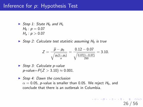
Inference for p: Hypothesis Test

I Step 1: State H0 and H1

H0 : p = 0.07Ha : p > 0.07

I Step 2: Calculate test statistic assuming H0 is true

Z =p̂ − p0√p0(1−p0)

n

=0.12− 0.07√

0.07(1−0.07)250

= 3.10.

I Step 3: Calculate p-valuep-value=P(Z > 3.10) ≈ 0.001.

I Step 4: Dawn the conclusionα = 0.05, p-value is smaller than 0.05. We reject H0, andconclude that there is an outbreak in Columbia.

26 / 56

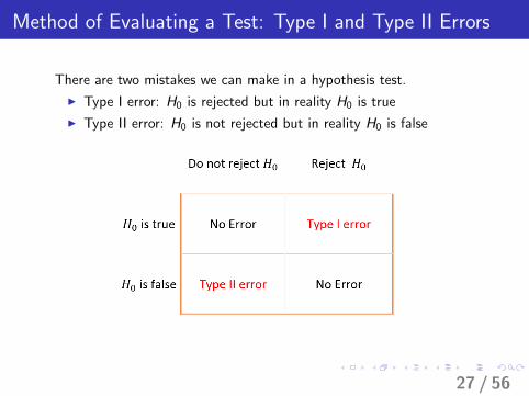
Method of Evaluating a Test: Type I and Type II Errors

There are two mistakes we can make in a hypothesis test.

I Type I error: H0 is rejected but in reality H0 is true

I Type II error: H0 is not rejected but in reality H0 is false

27 / 56

Controlling Risk

I The probability of type I error is denoted by α (same as thelevel of significance), i.e.,

α = Prob (reject H0|H0 is true).

I The type II error is denoted by β, i.e.,

β = Prob (fail to reject H0|Ha is true at some value).

I The idea situation is both type I and type II error is 0, whichmeans we can always make correct decision. However, onlyoracle knows the true. For us, every decision we make will haveassociated error probability.

28 / 56

Controlling Risk Cont’d

I In practice, if we try to decrease the type I error, the type II errorwill increase, and vice versa. Remember, there is no free lunch!

I Researchers should consider the consequences of type I errorand type II errors to help determine significance level.

I Example: An environmentalist takes samples at a nearby river tostudy the average concentration level of a contaminant. Hewants to find out, using a 0.1 level of significance, if the averageconcentration level exceeds the acceptable level for safelyconsuming fish from the river.

29 / 56

Controlling Risk Cont’d

I Describe a Type I error for this problem and the potentialconsequence.

I Describe a Type II error for this problem and the potentialconsequence.

30 / 56

Inference of Population Mean

I For binary random variable, we have discussed how to estimate thepopulation proportion using point estimate and confidence interval.

I Moreover, we built a 4-step procedure to test the hypothesiscorresponding to the population proportion.

I Now, it’s time to move on to the case when the random variable isnumerical and learn some method to guess population mean µ in theproper way.

31 / 56

Sampling distribution of Y

I Recall sample mean Y is a reasonable point estimator of thepopulation mean µ.

I RESULT: Suppose Y1,Y2, . . . ,Yn is a random sample from aN (µ, σ2) distribution. Then the sample mean Y has thefollowing sampling distribution:

Y ∼ N (µ,σ2

n)

I The above result reminds usI Y is an unbiased estimator of µ.I se(Y ) = σ/

√n

32 / 56

Example

I Let Y =time (in seconds) to react to brake lights duringin-traffic driving.

I We assume Y ∼ N (µ = 1.5, σ2 = 0.16). We call this thepopulation distribution.

I Suppose that we take a random sample of n = 5 drivers withtimes Y1, . . . ,Y5. What is the distribution of the sample meanY ?

33 / 56

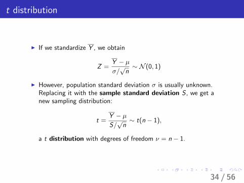
t distribution

I If we standardize Y , we obtain

Z =Y − µσ/√n∼ N (0, 1)

I However, population standard deviation σ is usually unknown.Replacing it with the sample standard deviation S , we get anew sampling distribution:

t =Y − µS/√n∼ t(n − 1),

a t distribution with degrees of freedom ν = n − 1.

34 / 56

t distribution

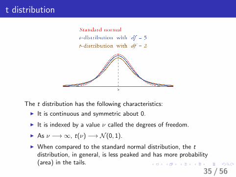
The t distribution has the following characteristics:

I It is continuous and symmetric about 0.

I It is indexed by a value ν called the degrees of freedom.

I As ν −→∞, t(ν) −→ N (0, 1).

I When compared to the standard normal distribution, the tdistribution, in general, is less peaked and has more probability(area) in the tails.

35 / 56

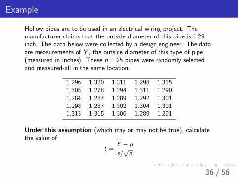
Example

Hollow pipes are to be used in an electrical wiring project. Themanufacturer claims that the outside diameter of this pipe is 1.29inch. The data below were collected by a design engineer. The dataare measurements of Y , the outside diameter of this type of pipe(measured in inches). These n = 25 pipes were randomly selectedand measured-all in the same location.

1.296 1.320 1.311 1.298 1.3151.305 1.278 1.294 1.311 1.2901.284 1.287 1.289 1.292 1.3011.298 1.287 1.302 1.304 1.3011.313 1.315 1.306 1.289 1.291

Under this assumption (which may or may not be true), calculatethe value of

t =Y − µs/√n

36 / 56

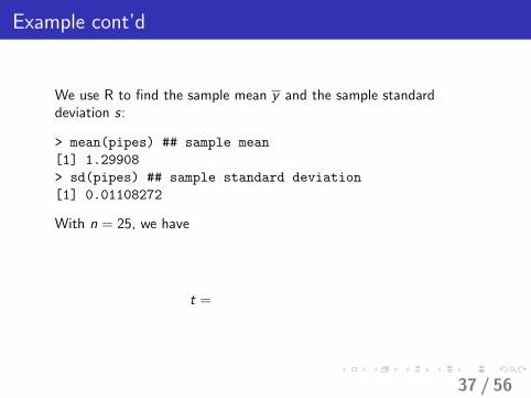
Example cont’d

We use R to find the sample mean y and the sample standarddeviation s:

> mean(pipes) ## sample mean

[1] 1.29908

> sd(pipes) ## sample standard deviation

[1] 0.01108272

With n = 25, we have

t =

37 / 56

Example cont’d

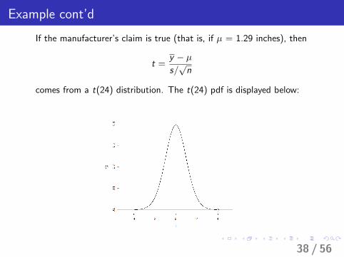
If the manufacturer’s claim is true (that is, if µ = 1.29 inches), then

t =y − µs/√n

comes from a t(24) distribution. The t(24) pdf is displayed below:

38 / 56

Example cont’d

Key question: Does t = 4.096 seem like a value you would expectto see from this distribution? If not, what might this suggest? Recallthat t was computed under the assumption that µ = 1.29 inches(the manufacturer’s claim).

QUESTION: The value t = 4.096 is what percentile of the t(24)distribution?

> pt(4.096,24)

[1] 0.9997934

39 / 56

Normal quantile-quantile (qq) plots

I Recall if Y1, . . . ,Yn is a random sample from a N (µ, σ2)distribution, then

t =Y − µs/√n∼ t(n − 1)

I An obvious question arises: “What if Y1, . . . ,Yn arenon-normal?”

I Answer: The t distribution result still approximately holds. Thatis, the t distribution is robust to the normality assumption.

I How to assess the normal distribution assumption? Normalquantile-quantile (qq) plot

40 / 56

Normal quantile-quantile (qq) plots cont’d

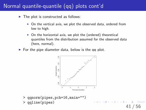
I The plot is constructed as follows:

I On the vertical axis, we plot the observed data, ordered fromlow to high.

I On the horizontal axis, we plot the (ordered) theoreticalquantiles from the distribution assumed for the observed data(here, normal).

I For the pipe diameter data, below is the qq plot.

−2 −1 0 1 2

1.28

1.29

1.30

1.31

1.32

Theoretical Quantiles

Sam

ple

Qua

ntile

s

> qqnorm(pipes,pch=16,main="")

> qqline(pipes)41 / 56

Normal quantile-quantile (qq) plots cont’d

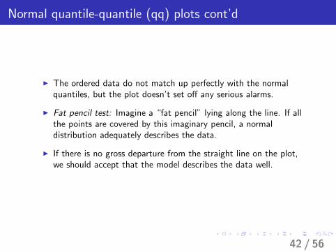
I The ordered data do not match up perfectly with the normalquantiles, but the plot doesn’t set off any serious alarms.

I Fat pencil test: Imagine a “fat pencil” lying along the line. If allthe points are covered by this imaginary pencil, a normaldistribution adequately describes the data.

I If there is no gross departure from the straight line on the plot,we should accept that the model describes the data well.

42 / 56

CI for µ. Assume normality and KNOWN σ2

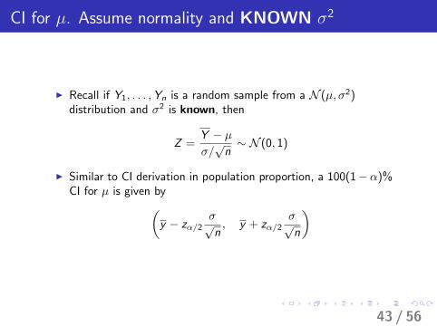
I Recall if Y1, . . . ,Yn is a random sample from a N (µ, σ2)distribution and σ2 is known, then

Z =Y − µσ/√n∼ N (0, 1)

I Similar to CI derivation in population proportion, a 100(1−α)%CI for µ is given by(

y − zα/2σ√n, y + zα/2

σ√n

)

43 / 56

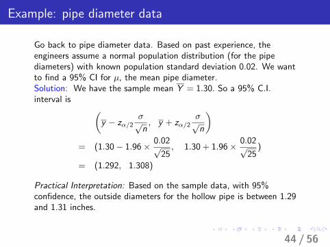
Example: pipe diameter data

Go back to pipe diameter data. Based on past experience, theengineers assume a normal population distribution (for the pipediameters) with known population standard deviation 0.02. We wantto find a 95% CI for µ, the mean pipe diameter.Solution: We have the sample mean Y = 1.30. So a 95% C.I.interval is (

y − zα/2σ√n, y + zα/2

σ√n

)= (1.30− 1.96× 0.02√

25, 1.30 + 1.96× 0.02√

25)

= (1.292, 1.308)

Practical Interpretation: Based on the sample data, with 95%confidence, the outside diameters for the hollow pipe is between 1.29and 1.31 inches.

44 / 56

CI for µ. Assume normality and UNKNOWN σ2

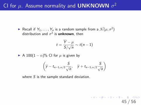
I Recall if Y1, . . . ,Yn is a random sample from a N (µ, σ2)distribution and σ2 is unknown, then

t =Y − µS/√n∼ t(n − 1)

I A 100(1− α)% CI for µ is given by(y − tn−1,α/2

S√n, y + tn−1,α/2

S√n

)where S is the sample standard deviation.

45 / 56

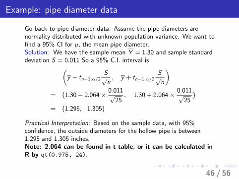
Example: pipe diameter data

Go back to pipe diameter data. Assume the pipe diameters arenormality distributed with unknown population variance. We want tofind a 95% CI for µ, the mean pipe diameter.Solution: We have the sample mean Y = 1.30 and sample standarddeviation S = 0.011 So a 95% C.I. interval is(

y − tn−1,α/2S√n, y + tn−1,α/2

S√n

)= (1.30− 2.064× 0.011√

25, 1.30 + 2.064× 0.011√

25)

= (1.295, 1.305)

Practical Interpretation: Based on the sample data, with 95%confidence, the outside diameters for the hollow pipe is between1.295 and 1.305 inches.Note: 2.064 can be found in t table, or it can be calculated inR by qt(0.975, 24).

46 / 56

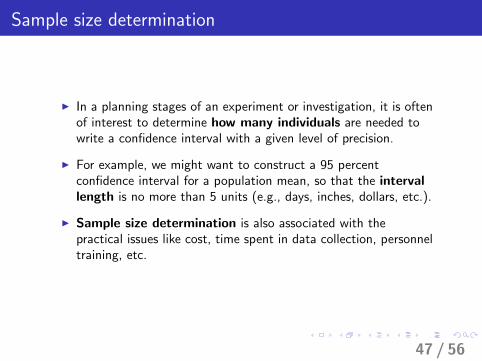
Sample size determination

I In a planning stages of an experiment or investigation, it is oftenof interest to determine how many individuals are needed towrite a confidence interval with a given level of precision.

I For example, we might want to construct a 95 percentconfidence interval for a population mean, so that the intervallength is no more than 5 units (e.g., days, inches, dollars, etc.).

I Sample size determination is also associated with thepractical issues like cost, time spent in data collection, personneltraining, etc.

47 / 56

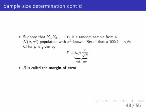
Sample size determination cont’d

I Suppose that Y1,Y2, . . . ,Yn is a random sample from aN (µ, σ2) population with σ2 known. Recall that a 100(1− α)%CI for µ is given by

Y ± zα/2σ√n︸ ︷︷ ︸

=B, say

I B is called the margin of error.

48 / 56

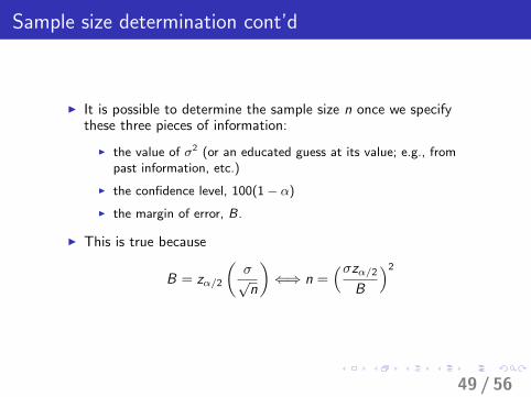
Sample size determination cont’d

I It is possible to determine the sample size n once we specifythese three pieces of information:

I the value of σ2 (or an educated guess at its value; e.g., frompast information, etc.)

I the confidence level, 100(1− α)

I the margin of error, B.

I This is true because

B = zα/2

(σ√n

)⇐⇒ n =

(σzα/2B

)2

49 / 56

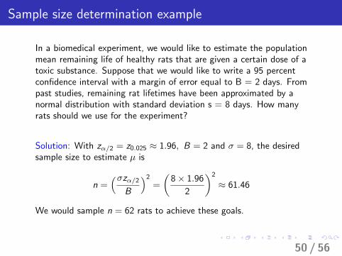
Sample size determination example

In a biomedical experiment, we would like to estimate the populationmean remaining life of healthy rats that are given a certain dose of atoxic substance. Suppose that we would like to write a 95 percentconfidence interval with a margin of error equal to B = 2 days. Frompast studies, remaining rat lifetimes have been approximated by anormal distribution with standard deviation s = 8 days. How manyrats should we use for the experiment?

Solution: With zα/2 = z0.025 ≈ 1.96, B = 2 and σ = 8, the desiredsample size to estimate µ is

n =(σzα/2

B

)2=

(8× 1.96

2

)2

≈ 61.46

We would sample n = 62 rats to achieve these goals.

50 / 56

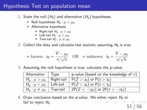
Hypothesis Test on population mean

1. State the null (H0) and alternative (Ha) hypotheses.I Null hypothesis H0 : µ = µ0

I Alternative hypothesisI Right-tail Ha : µ > µ0I Left-tail Ha : µ < µ0I Two-tail Ha : µ 6= µ0

2. Collect the data and calculate test statistic assuming H0 is true.

σ known: z0 =Y − µ0

σ/√n

OR σ unknown: t0 =Y − µ0

s/√n

3. Assuming the null hypothesis is true, calculate the p-value.

Alternative Type p-value (based on the knowledge of σ)Ha : µ > µ0 Right-tail P(Z > z0) or P(t > t0)Ha : µ < µ0 Left-tail P(Z < z0) or P(t < t0)Ha : µ 6= µ0 Two-tail 2P(Z < −|z0|) or 2P(t < −|t0|)

4. Draw conclusion based on the p-value. We either reject H0 orfail to reject H0.

51 / 56

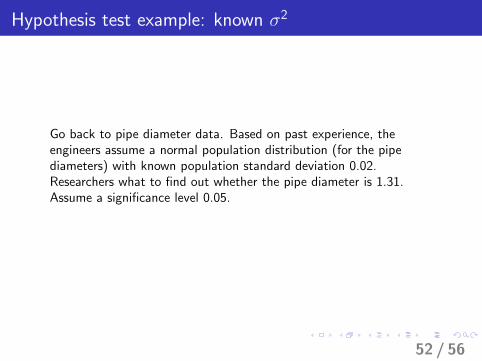
Hypothesis test example: known σ2

Go back to pipe diameter data. Based on past experience, theengineers assume a normal population distribution (for the pipediameters) with known population standard deviation 0.02.Researchers what to find out whether the pipe diameter is 1.31.Assume a significance level 0.05.

52 / 56

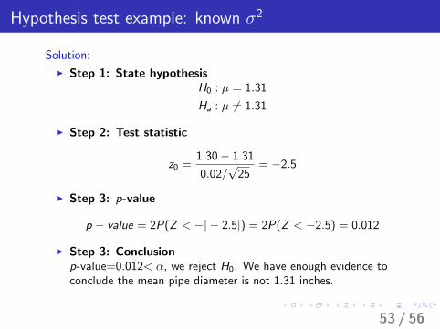
Hypothesis test example: known σ2

Solution:

I Step 1: State hypothesisH0 : µ = 1.31

Ha : µ 6= 1.31

I Step 2: Test statistic

z0 =1.30− 1.31

0.02/√

25= −2.5

I Step 3: p-value

p − value = 2P(Z < −| − 2.5|) = 2P(Z < −2.5) = 0.012

I Step 3: Conclusionp-value=0.012< α, we reject H0. We have enough evidence toconclude the mean pipe diameter is not 1.31 inches.

53 / 56

Hypothesis test example: unknown σ2

Go back to pipe diameter data. Assume the pipe diameters arenormality distributed with unknown population variance. Researcherswhat to find out whether the pipe diameter is less than 1.308.Assume a significance level 0.05.

54 / 56

Hypothesis test example: unknown σ2

Solution:

I Step 1: State hypothesis

I Step 2: Test statistic

I Step 3: p-value

I Step 3: Conclusion

55 / 56

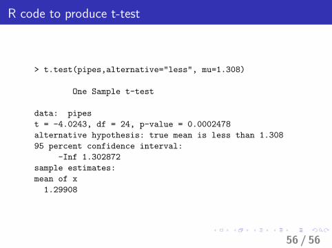
R code to produce t-test

> t.test(pipes,alternative="less", mu=1.308)

One Sample t-test

data: pipes

t = -4.0243, df = 24, p-value = 0.0002478

alternative hypothesis: true mean is less than 1.308

95 percent confidence interval:

-Inf 1.302872

sample estimates:

mean of x

1.29908

56 / 56