This content has been downloaded from IOPscience. Please scroll down to see the full text.

Download details:

This content was downloaded by: christ

IP Address: 134.58.253.57

This content was downloaded on 12/11/2015 at 07:24

Please note that terms and conditions apply.

Statistical forces from close-to-equilibrium media

View the table of contents for this issue, or go to the journal homepage for more

2015 New J. Phys. 17 115006

(http://iopscience.iop.org/1367-2630/17/11/115006)

Home Search Collections Journals About Contact us My IOPscience

New J. Phys. 17 (2015) 115006 doi:10.1088/1367-2630/17/11/115006

PAPER

Statistical forces from close-to-equilibriummedia

UrnaBasu1,2, ChristianMaes2 andKarelNetočný31 SISSA, Trieste, Italy2 Instituut voor Theoretische Fysica, KULeuven, Belgium3 Institute of Physics, Academy of Sciences of theCzechRepublic, Prague, Czech Republic

E-mail: netocny@fzu.cz

Keywords: statistical forces, irreversible thermodynamics,McLennan ensemble, frenometer,MINEP

AbstractWediscuss the physicalmeaning and significance of statistical forces on quasi-static probes infirstorder around detailed balance for drivenmedia. Exploiting the quasi-static energetics and thestructure of (McLennan) steady nonequilibrium ensembles, wefind that the statistical force obtains anonequilibrium correction deriving from the excess work of driving forces on themedium in itsrelaxation after probe displacement. This reformulates, within amore general context, the recentresult byNakagawa (2014 Phys. Rev.E 90 022108) on thermodynamic aspects of weakly none-quilibrium adiabatic pumping. It also proposes a possible operational tool for accessing some excessquantities in steady state thermodynamics. Furthermore, we show that the point attractors of a(macroscopic) probe coupled to aweakly drivenmedium realize the predictions of theminimumentropy production principle. Finally, we suggest amethod tomeasure the relative dynamical activitythrough different transition channels, via themeasurement of the statistical force induced by a suitabledriving.

Statistical forces are responsible in thermodynamics for generating transport of energy,momentumormatter asa result of the irreversible tendency to approach equilibrium [1]. They can be realized as truemechanical forcesby coupling a probe to themacroscopicmedium. The probe can itself be amacroscopic device like awall or apistonwith pressure as the statistical force. Another example are elastic forces which can be thought of asentropic forceswhen all interactions are ignored, working simply by the power of large numbers [2]. For our set-up (figure 1(a))wehave inmind a dilute suspension of colloids (=probe particles) in afluid (=medium)withmutual coupling, i.e., both colloid and fluid react to each other as dictated from an interaction potential.Weassume however that the colloid is quasi-static,meaning that its characteristic time ismuch longer than that ofthefluid. The resulting effective dynamics of the colloid picks up various aspects of the fluid; there are thefriction and the noise as usual formotion in a thermal bath, but because of our assumption of infinite time-scaleseparationwe concentrate here exclusively on the systematic forcewhich is the statistical average over the fluiddegrees of freedomof themechanical force on the colloid; see [3, 4] for further discussion on friction and noisein nonequilibriummedia. The general question concerning thermodynamics of active or drivenmedia is ofmuch current interest, e.g. for exploring the validity of equations of state in nonequilibrium [5–8].

For a probe in contact with an equilibrium reservoir the free energy is a potential for statistical forces. Thepresent paper studies these forces for reservoirs that are subject toweak driving. By the latter wemean that thefluid particles are undergoing rotational (nonconservative) forces with dissipation in yet another backgroundenvironment thatwill just be represented by its temperature; see figure 1(a). Themain question is to see how thatnonequilibrium feature corrects the gradient statistical force derived from the (equilibrium) free energy. Or,vice versa, how the force on the colloid teaches us about irreversible thermodynamic features of the fluid. Theresult is that to linear order in the amplitude of the rotational forces thework on the probe equals the excesswork done on thefluid by the rotational forces in its relaxation to the new stationary condition corresponding tothe slightly displaced probe. A similar result was already obtained in [9] in the context of cyclic adiabaticpumping.

OPEN ACCESS

RECEIVED

18May 2015

REVISED

7October 2015

ACCEPTED FOR PUBLICATION

13October 2015

PUBLISHED

10November 2015

Content from this workmay be used under theterms of theCreativeCommonsAttribution 3.0licence.

Any further distribution ofthis workmustmaintainattribution to theauthor(s) and the title ofthework, journal citationandDOI.

© 2015 IOPPublishing Ltd andDeutsche PhysikalischeGesellschaft

Excess quantities are omnipresent in discussions on steady state thermodynamics. Their origin is theoretical,trying to distinguish steady state effects from transient effects also for nonequilibrium fluids. Indeedwhendriven, the fluid obtains a stationary dissipationwith somemean entropy production rate in the environment.However, as some external parameters change in time, relaxational processes of the nonequilibrium fluidwillalso contribute to (excess) dissipation. The origin of such decomposition, housekeeping versus excessdissipation, is probably found in thework of Glansdorff and Prigogine [10, 11], but it has since been repeatedlystressed also inmore recent studies of steady state thermodynamics [12–16]. For example, for thermal propertiesof nonequilibrium systems one introduces the excess heat which defines nonequilibriumheat capacities [17, 18].One recurrent difficulty however is tofind a good operationalmeaning of these excess quantities. Nature doesnot dissipate the steady heat and the excess heat separately; similar for the notion of excess work. That is why itcan be useful tofind that the statistical force on a probe is directly related to excess work, at least close toequilibrium and for thermodynamic transformations controlled bymechanicalmotion of a probe.

A furthermotivation of the present work is to complete the close-to-equilibrium theory of steady statethermodynamics with the nature of statistical forces. Clearly and aswewill see in section 1 statistical forces enterin the First Law for the energy balance. They are therefore verymuch part of the theory of irreversiblethermodynamics for composed systems (here, probe plusfluid).Moreover, as is the content of section 4, thequestion appears inwhat sense these statistical forces realize theminimumentropy production principle; see[19]. In otherwords, whetherwe can understand statistical forces as theway inwhich systems achieveminimumentropy production rate. The answer is positive in the sense that indeed the very requirement ofminimalentropy production rate for the composed system again and also determines the statistical force in terms of theexcess work.

A third direction inwhich statistical forces are interesting, is that they are able tomake visible aspects of(time-symmetric) dynamical activity. That is not surprising because excess work involves the dynamics andhence, in contrast with the free energywhich is static, kinetic factors will be present in the statistical force.Webuild that into a ‘frenometer’ to get explicit information about the relative dynamical activity through reactivitychannels; see section 5.

We begin the paperwith a thermodynamic approach based on specifying the energy balance close-to-equilibrium.Wefind the relation between excess work of themedium, the force done on the probe and thenonequilibriumheat capacity. Section 2 gives the corresponding statisticalmechanical basis.We need theMcLennan ensemble theory to determine the correction to the equilibrium statistical forces. It gives a secondderivation of the result that relates excess work of themediumwith thework to displace the probe.We endsection 2with a discussion about the validity of our result when kinematical time reversal is included (like forunderdamped diffusions). Section 3 is devoted to a detailed illustration of the framework in context of a linearsystem. The relation between excess work and statistical forces is rederived using theminimum entropyproduction principle in section 4. The relation between statistical work and relative dynamical activity iscontained in section 5, suggesting as we alreadymentioned, a simple ‘frenometer’.

The present work follows and substantially extends [20]where themain idea has been reported.

Figure 1. (a)A slowprobe (light grey disc) is immersed in a nonequilibriummedium (green arrowed circles), in contact with anequilibrium reservoir (small blue circles). (b)Excess work V x, h( ) done by the driving forces in relaxing to the stationary conditionfor afixed probe postion x starting frommedium configuration η. Here Wx˙ denotes themean instantaneous power of the drivingforces.

2

New J. Phys. 17 (2015) 115006 UBasu et al

1. Energetics of irreversible thermodynamics

We refer tofigure 1(a) for a cartoon of three classes of particles. There is the probe onwhich a force is induced byits contact with amedium and a heat bath. Themedium is subject to nonequilibrium conditions and dissipatesinto the (equilibrium) heat bath at temperatureT. In general x denotes the ‘position’ (possiblymulti-dimensional) of the probe.With f the statistical force, the correspondingwork performed bymoving the probeis f xd .· The stationary energy of themediumwhen the probe is at x is denoted by E x .( ) Then, the quasi-staticenergetics (or ‘First law’) of the nonequilibriummedium is generally given by the balance equation for theenergy as

E x f x W x Q xd d 1ex ex= - + +( ) · đ ( ) đ ( ) ( )

where W exđ denotes the excess thermodynamicwork of the driving forces in themedium along the relaxationprocess that corresponds to the thermodynamic transformation x x xd , + T T Td , + and similarly

Qexđ is the (incoming) excess heat. Note that we speak about excesses because the stationarymedium constantlydissipates work into heat; excess is the extra corresponding to the transient process of reaching a new stationarycondition.We assume that the excess heat satisfies aClausius relation Q T S xdex =đ ( )withT the temperatureand S(x) can then be called the calorimetric entropy.We do not need its detailed expression here. Theassumption can be checked (aswe do in the next section 2) in the linear regime around thermodynamicequilibrium; the original proof is found in thework of Komatsu et al [15, 21].We define the free energy

x E x TS x = -( ) ( ) ( ) for which then, see also [15]

S T f x Wd d d . 2ex = - - +· đ ( )

By the (equilibrium)minimum free energy principle we know that there is no linear order correction in ord , meaning that in the considered linear regime x( ) coincides with the equilibrium free energy

x E x TSeq eq eq = -( ) ( ) , where the First Law for equilibrium combinedwith theClausius equality isE x f x T Sd d d .eq eq eq= - +( ) · Expanding around equilibrium, f f g ,eq= + S S s ,eq= + ˜ thefirst-ordercontributions yield zero free energy change and hence, within the first-order approximation

W s T g xd d . 3ex +đ ˜ · ( )

In particular for isothermal processes ( Td 0= ), wefind

g x Wd 4ex· đ ( )

for the nonequilibrium (tofirst order around equilibrium) component of statistical force in terms of the excesswork, whereas for xd 0= the excess work is related to the nonequilibrium entropy correction s ,˜ which is itselfrelated to the nonequilibriumheat capacity [17, 18].

Our observation on the absence of the first-order correction in the free energy provides a simple variation offormula (13) in [9] byNakagawa for thework transfer during cyclic adiabatic pumping in terms ofnonequilibrium (excess) heat into the driven system.However, we do not restrict ourselves to any specificprotocol of operation. Formula (4) gives a direct relation between themechanical force on the probe on the slowtime scale and the steady-state thermodynamic process in themediumon the fast time scale. Remark that theexcess quantities, though omnipresent in steady state thermodynamics, see the balance equation (1), are knownto be not easily accessible directly. Hence, formula (4) could be used to access some of the excess quantities in amechanical way.

In the next sectionwe give the statisticalmechanical basis for the above general thermodynamic arguments.

2. Statisticalmechanical approach

Weclosely follow the approach of Komatsu et al [22]. Yet we start from a general set-upwhich formalizes theidea of statistical force on quasi-static probes. Therewill be no need to introduce or indeed to specify the time-evolution except that we assume in general that themedium towhich the probe is coupled passes throughstationary states of some generic (McLennan) form.

We think of η as the collection of degrees of freedomof a drivenmedium. For the rest of the paperwe assumethese variables are even under kinematic time-reversal, so not containing velocity degrees of freedom as forexamplewith underdamped diffusions; the results do not change however in themore general case—seesection 2.3. For simple convenience we take themdiscrete so thatwe use sumswhen computing averages etc.Themediumparticles undergo rotational forces of order ε and they obtain a stationary regime by dissipatingheat into a thermal bath at temperatureT; we alsowrite T 1b = - setting Boltzmannʼs constant kB= 1. Eachstationary regime of themediumdepends on the position x of a slow probe. The probe is immersed in themedium and the contact ismodeled via a joint interaction potentialU x, h( )which by assumption also includesthe interaction among themediumparticles as well as the self-interaction of the probe if present. As themedium

3

New J. Phys. 17 (2015) 115006 UBasu et al

is supposed to bemacroscopic it is relevant to define the statistical force on the probe as the averagemechanicalforce

f x U x U x, , 5x x xxår h h h= - = -á ñ

h( ) ( ) ( ) ( ) ( )

where the average is over the steady nonequilibrium stationary distribution ρx of the η-medium atfixed x. Notethat the total system is composed (mediumparticles plus probe) butwework under the hypothesis that the η-variables are relaxingmuch faster.Whenwe apply that to the case of an equilibriummediumwe find thestandard result that the statistical force is given as the gradient of the free energy. In statisticalmechanical writingthat free energy is x T Zlog xeq = -( ) withZx the equilibriumpartition function corresponding to the η-mediumwhen in equilibriumwith fixed probe position x: the distribution is then given by the Boltzmann–Gibbsfactor U x Zexp , .x x

eqr h b h= -( ) { ( )}To go beyond equilibrium, we need information about ρx for determining (5).Wework under the condition

of local detailed balance for the nonequilibriummedium [23–26]which relates the probe-mediumdynamicswith the entropy fluxes into the environment (=a heat bath at temperatureT). By our assumption the drivingforces breaking the global detailed balance provide a contribution to the entropyfluxes proportional to somesmall parameter .e

Close to equilibrium themedium iswell described by theMcLennan stationary ensemble [27, 28]

1e . 6x

x

U V xML ,

r h = b h- +( ) ( )( )( )

HereV x, h( ) is the excess work of driving forces along the relaxation process started from ηwith xfixed havingzero expectation V 0xá ñ = under the stationary distribution ρx; seefigure 1(b) and (A.1) in appendix A for thedefinition.Note thatV is itself of order ε. It turns out that

O Z O, 7x x x xML 2 2r r e e= + = +( ) ( ) ( )

withZx the equilibriumpartition function (at ε= 0). Formula (6) describes the steady linear regime aroundequilibrium. For example, linear response formulæ can be derived from it; see [28].

Specific examples follow below in sections 3 and 5.

2.1.Deriving the energy balanceThe stationary energy E x U x= á ñ( ) changes as

U U U xd d d , .x xxå r h há ñ = á ñ +

h( ) ( )

Themedium is doingwork f xd· on the probe, hence

U f xd d 8xá ñ = - · ( )

mimicking (5) as themechanical energyU does not depend on temperature. The excess workwhen themediumrelaxes from the stationarity under x to the new stationarity under x xd+ reads

W x V x x Vd , d 9xxex år h h= + = á ñ

hđ ( ) ( ) ( ) ( )

wherewe have used V 0.xá ñ = Using that condition again andwriting V V xd d , ,xxå r h há ñ = - h ( ) ( ) the

(renormalized) First law (1) is verified by defining the excess heat as

Q x U V xd , . 10xex å r h h= +

hđ ( ) ( )( )( ) ( )

Let us nowuse the statisticalmechanical formulæ (6) and (7) towork in the linear regime, and use x xMLr r

to replace the stationary distribution in leading order around equilibrium. TheClausius equalityQ T S x Odex 2e= +đ ( ) ( )with entropy S x log ,x xå r h r h= - h( ) ( ) ( ) can be obtained directly from the

definitionswhen using theMcLennan distribution (6). The free energy equals

x U TS x T Z Olog 11xx

2 e= á ñ - = - + ( )( ) ( ) ( )

and indeed has no linear order correction. That verifies the hypotheses involved in the thermodynamicderivation of (3).We can however also give a direct derivation inserting (6) into (5), which comes next.

4

New J. Phys. 17 (2015) 115006 UBasu et al

2.2. Excesswork equals the nonequilibrium correction to statistical workWhen themediumundergoes nonequilibriumdriving, there is a new stationary nonequilibriumdensity,

h1 12x x xeq ⎡⎣ ⎤⎦r h r h h= +( ) ( ) ( ) ( )

in terms of a density hx (of order ε)with respect to the reference equilibriumdistribution. The equilibriumdistribution x

eqr h( ) satisfies the identity

TU x Z

1, log .x x x x x x

eq eq ⎡⎣⎢

⎤⎦⎥r h r h h = - + Î( ) ( ) ( )

Weobtain the statistical force f x T Z g xlogx x= +( ) ( ) bymultiplying the above relationwith x xeqr h r h( ) ( )

and summing over η. The nonequlibrium correction g(x) is then given in terms of the density hx defined in (12)above

g x T h T h . 13x x x x xxeq ,eqå h r h= - = - á ñ

h( ) ( ) ( ) ( )

Since h h 0x x xxeq ,eqå h r h = á ñ =h ( ) ( ) (from the normalization applied to (12)), for a small displacement xd

of the probe thework done is

g x x T h T hd . 14x x x x xx

deq

d,eqå h r h= - = - á ñ

h+ +( ) · ( ) ( ) ( )

When interested infirst order around equilibriumwe can aswell write

g x x T h Od 15x xx

d2e= - á ñ ++ ( )( ) · ( )

with respect to the stationary distribution of themedium in contact with an external thermal bath at temperature

T. TheMcLennan distribution (6) gives hT

V x O1

,x2h h e= - +( ) ( ) ( ) and combining that with (10)we

recover (4).

2.3. Including kinematical time-reversalThe result that certain excess quantities as encountered in steady state thermodynamics are accessible viamechanicalmeasurements, remains valid in a broader context than considered so far.We have inmind the caseofmediumvariables η containing velocity degrees of freedomor,more generally, dynamical degrees of freedomthat are not even under kinematic time-reversal.We indicate here brieflywhere some changes in the argumentswould occur.

First, the purely thermodynamic argument of section 1 does not change at all. The entropy Sused therewillhowever get a slightlymore general statisticalmechanical appearance than in section 2.1.We have to use thesymmetrized Shannon entropy introduced byKomatsu et al; see e.g. [15] for a recent review. Callingπ thekinematic time-reversal (likeflipping the sign of allmomenta) and assuming that the equilibrium reference isπ–invariant, ,x x

eq eqr ph r h=( ) ( ) wehave theClausius relation (infirst order ε around equilibrium)

Q T S x Odex 2e= +đ ( ) ( )with entropy S x1

2log .x x xå r h r ph r h= - +h( ) [ ( ) ( )] ( ) That relation again

follows by taking for xr h( ) theMcLennan distribution, but the excess workV x, h( ) does not appear directly inthe statistical weight. Rather, the nonequilibrium correction to the equilibriumdistribution has themore

general form hT

V x O1

, .x2h ph e= - +( ) ( ) ( ) Despite themodification of the entropy function, the formulas

(14) and (15) yield g x x V x x Od d , x 2h e= á + ñ +( ) · ( ) ( )without any change. SinceV x x V x x Od , d ,x x,eq 2h h eá + ñ = á + ñ +( ) ( ) ( ) still equals the excess work W xexđ ( ) for the transformation

x x xd ,+ we have checked that ourmain relation (4) indeed extends to thismore general case.

3. Linearmodel

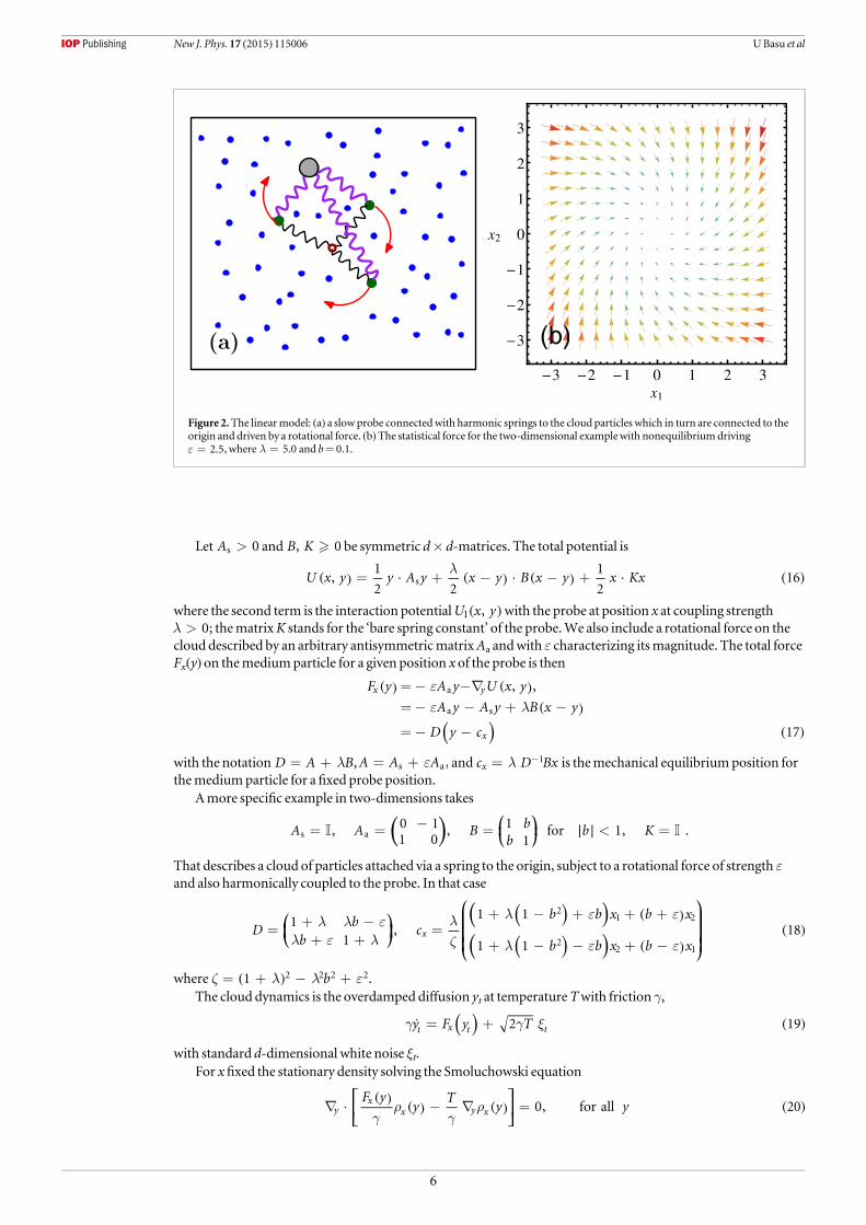
As an illustrationwe consider asmedium a cloud of non-interacting particles driven by linear rotational forcesand diffusivelymoving in a viscousfluid. The linearity is assumed also for the interactionwith the probe as wellas for a potential force trapping the cloud in a bounded region. It allows exact calculations and is a goodapproximation forweak nonlinearities.

The cloud consists ofmany particles fromwhich it willmake sense consider statistical average but aswe takethem independent, it suffices to consider just one of them. That generic particle lives in d-dimensionswithcoordinate y y y, , ;d1= ¼( ) weuse here y instead of η for better accordance with position degrees of freedom.See figure 2(a) for a d= 2-representation.

5

New J. Phys. 17 (2015) 115006 UBasu et al

Let A 0s > and B K, 0 be symmetric d× d-matrices. The total potential is

U x y y A y x y B x y x Kx,1

2 2

1

216s

l= + - - +( ) · ( ) · ( ) · ( )

where the second term is the interaction potentialU x y,I ( )with the probe at position x at coupling strength0;l > thematrixK stands for the ‘bare spring constant’ of the probe.We also include a rotational force on the

cloud described by an arbitrary antisymmetricmatrixAa andwith ε characterizing itsmagnitude. The total forceFx(y) on themediumparticle for a given position x of the probe is then

F y A y U x y

A y A y B x y

D y c

, ,

17

x y

x

a

a s

ee l

=- -=- - + -

=- -( )

( ) ( )( )

( )

with the notation D A B,l= + A A A ,s ae= + and c D Bxx1l= - is themechanical equilibriumposition for

themediumparticle for afixed probe position.Amore specific example in two-dimensions takes

A A B bb

b K, 0 11 0

, 11

for 1, .s a ⎜ ⎟⎛⎝

⎞⎠ = = - = < =( ) ∣ ∣

That describes a cloud of particles attached via a spring to the origin, subject to a rotational force of strength εand also harmonically coupled to the probe. In that case

Db

bc

b b x b x

b b x b x

11

,1 1

1 118x

21 2

22 1

⎛⎝⎜

⎞⎠⎟

⎛

⎝⎜⎜⎜

⎞

⎠⎟⎟⎟

l l el e l

lz

l e e

l e e= + -

+ +=

+ - + + +

+ - - + -

( )( )

( )( )

( )

( )( )

where b1 .2 2 2 2z l l e= + - +( )The cloud dynamics is the overdamped diffusion yt at temperatureTwith friction γ,

y F y T2 19t x t tg g x= +( )˙ ( )

with standard d-dimensional white noise ξt.For xfixed the stationary density solving the Smoluchowski equation

F yy

Ty y0, for all 20y

xx y x

⎡⎣⎢

⎤⎦⎥g

rg

r - =· ( ) ( ) ( ) ( )

Figure 2.The linearmodel: (a) a slowprobe connectedwith harmonic springs to the cloud particles which in turn are connected to theorigin and driven by a rotational force. (b)The statistical force for the two-dimensional examplewith nonequilibriumdriving

2.5e = , where 5.0l = and b= 0.1.

6

New J. Phys. 17 (2015) 115006 UBasu et al

is theGaussian density

y e 21xy c y c

T x x1

2r = - - G -( ) ( )( ) ( )·

where Tdet 2 d 1 2 p= G[ ( ) ( ) ] is the normalization andΓ is the (unique) positive symmetricmatrix satisfying

D D 2 221 1 G + G =- - ( )†

or, equivalently, the symmetric part of DG must equal ;2G see appendix B. In particular, ifD is normal in thesense that it commutes with its transpose, DD D D,=† † then the solution to (22) reads D A B.s s lG = = + Onthe other hand, for non-normalDʼs thematrixΓ does depend on .e Observe however also in (21) thetemperature-dependence which is always of the Boltzmann–Gibbs form, so that the stationary density for themedium can be seen as an equilibrium for the oscillator energy with ‘spring constant’Γ and equilibriumpositioncx. The (nonequilibrium) e-dependence sits in cx and for non-normalD also inΓ. Note by comparing (12)–(15)with (21), that we already know that the nonequilibrium correction in the statistical forcewill also betemperature-independent.

Coming back to the above two-dimensional example wefind thatD is non-normal whenever b 0.e ¹ Thestationary density is determined there by

bb

bb

11

1

11

23

⎛

⎝

⎜⎜⎜⎜

⎞

⎠

⎟⎟⎟⎟k

le l e

ll

l le l e

l

G =+ +

++

+ --

+

( )

( )( )

with 11

.2⎛

⎝⎜⎞⎠⎟k

el

= ++

The statistical force on the quasi-static probe follows from U x y B x y Kx, ,x l = - +( ) ( ) and equals

f x U x y y y

B c x Kx A KB D c Mx

, d ,

124

x x

x x1⎜ ⎟⎛

⎝⎞⎠

ò r

ll

=-

= - - = - + = --( )( ) ( ) ( )

( )

where M K B BD B K B A .2 1 1 1 1l l l l= + - = + +- - - -( ) Of course the contribution ofK is not statisticalandwas there as self-potential from the beginning. Note that the statistical force is temperature-independent. Asfor linear overdamped dynamics, rotational forces enter via asymmetricmatrices and it is indeed useful todecompose M M Ms a= + with M M M 2,s = +( )† M M M 2.a = -( )† The antisymmetric componentMa

quantifies the induced rotational part and is of order .2elContinuingwith the above two-dimensional example, we have that the antisymmetric part equals

Mb

bA

1

125a

2 2

2 2 2 2 a

el

l l e=

-

+ - +

( )( )

( )

and the symmetric part ofM obtains a second-order correctionwith respect to equilibrium,

M Kb b

b b

b b

b b

1 1 1

1 1 1

1 1 1 2 2 1

1 1 1 2 2. 26

s

2 2 2

2 2 2

2 2 2 2

2 2 2 2

⎛

⎝⎜⎜

⎞

⎠⎟⎟

⎛

⎝⎜⎜

⎞

⎠⎟⎟

lz

l e e

e l e

z

l l e l l e

l e l l e l

= ++ - + +

+ + - +

=+ + + - +

+ + + + -

( ) ( )( ) ( )( ) ( )

( ) ( )( )

( )( )

Such a renormalization of the ‘bare’ interaction constant due to couplingwith environment is often called a‘Lamb shift’; here we see how it obtains a nonequilibrium contribution of order O 2le( ) from the driving of themedium. Infigure 2(b)weplot the phase portrait of the statistical force under a specific choice of parameters.

The resultingmotion of the probe depends of course on still other aspects of themedium and bath. Therewill be friction and noise as further corrections to the statistical force, but for a quasi-static andmacroscopicprobe ofmassmwe simply put

mx f x Mx¨ here= = -( ) ( )

for its equation ofmotion.To obtain yet another representation of the statistical force we observe (see appendix B) that for (16),

U x y y c D y c c D y c x M x,1

2

1

2x x x xs a s= - - + - +( ) ( ) ( )( ) · · ·

7

New J. Phys. 17 (2015) 115006 UBasu et al

(with D Aa ae= ) and themean energy is

Ud

T x M x2

1

2. 27x

sá ñ = + · ( )

Combinedwith themedium’s stationary entropy

S xd D

Tlog

2

1

2log

det

2xx

d

sr

p= -á ñ = -

( )( )

( )

we obtain the nonequilibrium free energy

x U TS xD

Tx M x

1

2log

det

2

1

2. 28x

d

s

sp

= á ñ - = +( )

( ) ( )( )

· ( )

The latter is to be comparedwith its equilibrium counterpart

x T y

D

Tx M x

log e d ,

1

2log

det

2

1

2

U x y

d

eq,

s

s0

ò

p

=-

= +

b-

( )( )

( )·

( )

( )

with M K B BD B .s0

s1l l= + - -[ ]( ) Note that from theGibbs variational principle, x x ;eq ( ) ( ) their

difference comes from M M O .s s0 2e l= + ( )( )

As a consequence the statistical force (24) ismanifestly a sumof two contributions

f x x M x U M x. 29x xx

a a= - - = - á ñ -( ) ( ) ( )

The rotational force−Aay on themediumhas been transformed into (i) a shift in the free energywhich (still)determines the conservative component of the force, and (ii) an induced rotational force−Max. The totalnonequilibrium correction to the statistical force on the probe is then given by

g x M M x M x. 30s s0

a= - - -)(( ) ( )( )

According to the general theory the term M xa- corresponds to the excess work of the rotational forces on themedium, at least close to equilibrium aswe have argued in the previous sections.We now check that within thepresent linear framework that is in fact exactly (to all orders of ε) verified (but theMcLennan distribution (6) isnot exactly equal to (21)).

We need to calculate the excess workV x y, ,( ) first when starting themedium from fixed position y atfixedprobe position x.We follow the derivation in thefirst part of appendix A. The expected power of the total forceFx(y) on themediumparticle is equal to

w y F y F yT

F y1

31x x x y xg g

= + ( ) ( ) · ( ) · ( ) ( )

(see for example equation (III.5) in [28] or appendix A). Then, following (A.1)

U x y U V x y w y y y w t, , d . 32xx t

xx

x

00

⎡⎣ ⎤⎦ò- á ñ + = á = ñ -¥ ( )( ) ( ) ( )

After some computation (see appendix B)wefind the excess work due to the rotational force, starting from afixedmediumparticle position y given by

V x y y c y cT

U x y U,1

2 2Tr , , 33x x

x1= - W - - WG - + á ñ-( ) ( ) ( )( ) · ( ) ( )

whereΩ is a positive symmetricmatrix such that

D D 2 . 341 1 W + W =- -( ) ( )†

(WhenD is a normalmatrix, then D ,1 1sW =- -( ) and D .1

a2W = G - G- )

The averaged excess work (10), when the probe is shifted from x x xd + is

W x y y V x x y V x yd d , , .xex ò r= + -đ ( ) ( )[ ( ) ( )]

8

New J. Phys. 17 (2015) 115006 UBasu et al

Wehave, from (33), to linear order in xd

W x U x U x

M x x Mx xM x x

d d

d dd . 35

xx

xxex

s

a

= á ñ - á ñ= -=-

đ ( ) · ·· ·

· ( )

Thus the excess work dissipated by themediumdue to the rotational force is equal to thework done on the probeby the rotational component of the statistical force when the probe position is shifted by an amount xd .

For the two-dimensional example wefind

bb

bb

11

11

⎛

⎝

⎜⎜⎜⎜

⎞

⎠

⎟⎟⎟⎟

le l e

ll

l le l e

l

W =+ +

++

+ --

+

( )

( )

and by comparingwith (23)we check the relation kW = G (moreover, D DGW = † )whichmeans that thestationary distribution of the cloud is given by an exact variant of theMcLennan ensemble

y U V x y Texp , ,x effr µ - +( ) [ ( )( ) ] with themodified potentialU+V and the ‘renormalized’ temperatureTeff = T T O .2k e= + ( ) As a consequence the two-dimensionalmodel satisfies the exact generalized Clausiusrelation Qex =đ T Sdeff (with respect to all possible thermodynamic transformations)where S x =( ) log x

xr-á ñis the stationary (Shannon) entropy.

4. Realizingminimumentropy production

In that same linear regime, statistical forces should reflect the tendency of the compound system (probe plusnonequilibriummedium) to reach the condition ofminimumentropy production rate (MINEP), [19], valid forclose-to-equilibriummedia with degrees of freedom that are even under kinematic time-reversal.We shownowthat the opposite also holds giving a third proof of (4): requiringMINEP implies that thework needed tomovethe probe over xd equals the change in equilibrium free energy plus excess work done by the nonconservativeforces on themedium to relax from the old stationary condition xr to the newone described by .x xdr +

4.1.Minimal nonequilibrium free energyBeforewe go to the actual application it is useful to derive an alternative (but equivalent) formulation of theminimumentropy production principle in terms of a nonequilibrium free energy functional.

Supposewe have statesσ (theywill be the states x,s h= ( ) of our compound system) and probabilitydistributionsμ on them. There is a driven processσt that satisfies the condition of local detailed balance. There isa unique stationary distribution ρ and obviously there is a trivial variational principle s 0m r( ∣ ) with equalityonly ifμ= ρ in terms of the relative entropy s logåm r m s m s r s= s( ∣ ) ( ) [ ( ) ( )] (for simplicity we take here

finite irreducibleMarkov processes). That variational formula starts being useful if log r s( ) has a (thermo)dynamicalmeaning. That is certainly the case at equilibriumbut also near equilibriumwhere OML 2r r e= + ( )in (6) is expressed in terms of energy and excess work. If wefindμ thatminimizes

s U Vlog log 0 36ML å åm r m s m s b m s s= + + +s s

( ) ( ) ( ) ( )( )( ) ( )

then (obviously) MLm r= and O 2m r e= + ( ) is a perfect linear order approximation to the true stationarydistribution. In the expression (36)we recognize the time-integrated entropy production for the process relaxingfromμ versus from theMcLennan distribution. That is because there

U V Slog .ML ML åb s r s r= - + +s( )( ) ( ) ( ) In that sensewe do exactly what theminimumentropy

production is doing, and in fact by requiring t sd d 0t tML

0 m r =( ∣ ) wewould even recover it in its usualinstanteneous version, [19].

Let us still rewrite (36) using the variational nonequilibrium free energy functional [29]

U V T S . 37neq åm s m s m= + -s

( ) ( )( ) ( ) ( ) ( )

At stationarityμ= ρ it coincides with the usual free energy functional U T S ,neq r r r= = á ñ -( ) ( ) ( ) sinceV 0,á ñ = and T log .neq

ML r = -( ) Furthermore, the positivity in (36) gives the variational principle

38neq neqML m r( )( ) ( )

with equality for O .ML 2m r r e= = + ( ) That is the free energy version ofMINEP: correct tofirst order ε thestationary distribution is the one that has lowest (nonequilibrium) free energy. Note also that r =( )

T Z Olog 2e- + ( ) and Vå m s s =s ( ) ( ) O 2e( )whenever O1 .m r e= + ( ) To the best of our knowledgethat formulation is new and especially useful for work-considerations as arise in the context of the present paper.

9

New J. Phys. 17 (2015) 115006 UBasu et al

4.2. Application to the probe-medium systemThe previous principle will be applied to the compound systemof probe plusmedium.Wemake however anadditional simplifying assumption, that we can characterize the statistical force at probe position x* byfindingthe constant forceB so thatwhen applyingB to the probe it actually relaxes to position x* as unique attractor andfixed point. Then, f x B;* = -( ) in otherwords,B exactly cancels the statistical force at steady position x .* Wenow consider themodified dynamics with that additional constant forceB on the probe andwe require that

x x x, x* *r h d r h= -( ) ( ) ( ) is the stationary distribution (always taken tofirst order in ò). That requirementwill be implemented by the free energy principle (orMINEP) (38).

Let us take as test-distribution x x z, zm h d r h= -( ) ( ) ( ) that would put the probe at z and take theMcLennan distribution ρz for themedium.Wenowwrite for that choice zneq neq m =( ) ( )which from (37)becomes

z B z U z TS W, zz

z xneq

:

ex

* òh r= - + á ñ - +

g ( ) · ( ) ( ) đ

where the last line-integral gives the excess workwhenmoving from z to x .* The principle (38) tells us that

B z U z TS W

B x U x TS B x x

,

, 39

zz

z x

xx

:

ex

eq* * * *

*

**

òh r

h r

- + á ñ - +

- + á ñ - = - +

g

( ) ( )· ( ) ( ) đ

· ( ) · ( )

wherewe inserted (correct tofirst order) the equilibrium free energy.We insert z x xd* *= + for smalldeviations around the attractor and find at theminimum

x W x B xd deqex* * * - =( ) ( )đ ·

which is again the sought result as B f x .*= - ( ) Supposing there is a unique x* at which f x 0,* =( ) that point ischaracterized byminimizing the nonequilibrium free energy .neq

For example, when two reservoirs are inmechanical contact, separated by a piston, the pistonwillmove toequalize the two pressures but the pressure is not just the derivative of the equilibrium free energy; onewill needto estimate the change in excess work under variations of the piston position.More specifically, consider a gas ina vessel divided into two compartments with volumesΛ1+Λ2=Λ via amovable piston, under isothermalconditions. If we start ‘stirring’ the gas in compartment 1, the piston getsmoving to continuously decrease thenonequilibrium free energy

W, 40neq 1 2 1 1 2 2 1ex

1

òL L = L + L -L( ) ( ) ( ) đ ( )

until it attainsminimum. The latter of course corresponds to equalizing pressures P1=P2 withP1 obtaining anonequilibrium correction, P Wd d d .1 1 1

ex1= - L + Lđ

Note that here againwe have considered the physical context of even degrees of freedom for themedium. Asis known, theminimumentropy production principle does not applywith velocity degrees of freedom; see e.g.[19]. Yet, themathematics and the formal arguments as presented above remain of course valid as such, althoughin that case of non-even degrees of freedomwithout a direct physical interpretation.

5.Measuring dynamical activity

Dynamical activitymeasures the time-symmetric current or the number of transitions in a given space-timewindow. It is the change in that activity when perturbing the system, or the relative activity when comparingdifferent transition paths, thatmatters in response theory [30]. In fact, also for detailed balance dynamics, thedynamical activity appears important for understanding aspects of jamming and glass transitions [31, 32].However, dynamical activity is difficult to access directly. Herewe look into a toy example demonstrating hownonequilibrium statistical forces could be used to (indirectly)measure the relative activity, at least in the case of asimple state-space geometry.

Assumewe have an equilibrium systemof noninteracting particles the configuration space of which splitsinto two parts,A andB, connected through a two-channel bottleneck only; see figure 3—we call them the+ and− channel.Wewant tofind outwhich of the two channels ismore ‘open’ in terms of their relative dynamicalactivities. The idea is to connect this question to the problemof how statistical forces respond to switching on aweak nonequilibrium force in the bottleneck.

The bottleneck consists of a pair of (single-particle) transitions A BA B, s s Î+ -

with rates

k U U, exp2

oA B

oA B⎜ ⎟⎛

⎝⎞⎠s s g

bs s= - ( ) [ ( ) ( )] respectively k U U, exp

2.o

B Ao

B A⎜ ⎟⎛⎝

⎞⎠s s g

bs s= - ( ) [ ( ) ( )] The

rest of the system is arbitrary up to that the transitions satisfy detailed balancewith potentialU and

10

New J. Phys. 17 (2015) 115006 UBasu et al

k , 0o h h¢ =( ) whenever η, h¢ do not belong either both toA or both toB.We are to determine the dynamicalactivitiesD± defined as themean equilibrium frequency of transitions along the channels±. Fromdetailedbalance

D

D

k k

k k

, ,

, ,. 41

Ao

A B Bo

B A

Ao

A B Bo

B A

o

o

eq eq

eq eq

r s s s r s s s

r s s s r s s sgg

=+

+=+

-

+ +

- -

+

-

( ) ( ) ( ) ( )( ) ( ) ( ) ( )

( )

Such a relative dynamical activity and its further dependence on nonequilibriumparameters is an example ofwhatwe callmore generally frenetic aspects, to contrast it with entropic features. In that way, the set-up infigure 3 represents a frenometer aswe now show.

Now enters the interactionwith a probe. Therefore, we let the energyU also depend on the position x of theprobe. The equilibrium statistical force on the probe is derived from the free energy. The partition function is thesumover all states, Z eA B A B

U x, ,

,å= hb h

Î- ( ) and that force equals

f T Z Z

f f

log ,

, 42

x A B

A A B B

eq

r r

= +

= +( )

( )

where f T ZlogA B x A B, ,= is themean force fromA andB, respectively, and Z Z ZA B A B A B, ,r = +( ) is theproportion of time the equilibrium system spends in each compartment.

In order tomeasure the relative activityD+ /D− , we drive the systemout of equilibriumby applying alocal nonpotential force whichmodifies the transition rates in the bottleneck to

k

k

, e ,

, e . 43

A BU x U x

B AU x U x

, ,

, ,

A B

B A

2

2

⎡⎣ ⎤⎦⎡⎣ ⎤⎦

s s g

s s g

=

=

s s e

s s e

-

-

b

b

( ) ( )

( ) ( )( )

( ) ( )

Apossible e-dependence of the kinetic factors g is allowed but irrelevant for linear order calculations; seebelow in (47) and the dependence on the parameter b infigure 3.We shownext that the nonequilibriumcorrection to the statistical force gives information aboutD+ /D− .

An immediate effect of turning on the drive is a redistribution of the particles, described to linear order in εby theMcLennan ensemble (6). For theV x, h( ) therewe need thework performed by the applied force alongthose parts of the relaxation trajectories that pass the bottleneck. All trajectories, say originating frompartA,have to pass through the ‘port’ As in order to access the bottleneck, and since no other transitions contribute todissipatedwork but the two special channels± ,V x V, A B,h =( ) is constant inside bothA andB. A calculation tolinear order (appendix A) yields

V VD D

D D, 44A B ex x- = =

-+

+ -

+ -( )

suppliedwith the normalization condition Z V Z V 0.A A B B+ = The difference V VA B- can be detected as anonequilibrium correction to the statistical force acting on the external slowparticle. By formula (13) and sinceh V x O, ,x

2h b h e= - +( ) ( ) ( ) that correction equals

Figure 3. Frenometer: (a) schematic representation of the two types of configurations connected through a two-channel transitionpath. (b)The nonequilibrium correction to the statistical force for the toymodel (for afixed x=π/2.) as a function of the driving εthrough the bottleneck for two different values of b= 1,2. and ξ= 0.1.We can read the relative dynamical activity in equilibrium fromthe slope. The inset shows the same correction g(x) as a function of x for a fixed 0.2e = and different ξ= 0.1,0.5.Here b= 1.

11

New J. Phys. 17 (2015) 115006 UBasu et al

g x V V x V x

VZ

Z ZV

Z

Z Z

Z Z

Z ZO

, ,

2. 45

xx

Ax x

Bx x

A xA

A BB x

B

A B

xA B

A B

,eq eq eq

2

⎛⎝⎜

⎞⎠⎟

⎛⎝⎜

⎞⎠⎟

⎛⎝⎜

⎞⎠⎟

å åh r h h r h

e xe

= á ñ = - -

=- +

- +

=- -+

+

h hÎ Î

( )

( ) ( ) ( ) ( ) ( )

( )

In terms of the (equilibrium) occupations and statistical forces associatedwithA respectivelyB, thenonequilibrium correction to the statistical force takes the form

g f f O . 46B A A B2exb r r e= - +( ) ( ) ( )

Hence, the channel-asymmetry factor ξ, characterizing the relative importance (in terms of dynamical activity)of the two channels, can be evaluated from thefirst order correction of the statistical force. It determines theslope in figure 3(b) in the close-to-equilibriumdependence of the statistical force on the nonequilibriumamplitude ε given that we know the equilibrium values fA, B and ρA, B.

For illustrationwe take a simple toy systemwhere bothA andB are two three-state rotators with states ηA,B=− 1, 0, 1 with bottleneck statesσA= 1A andσB= 1B connected by two channels. The probe is connected tothe rotators via interaction energy

U x x x x x, sin 2 cos cos 2 sin .A B,2

,2⎡⎣ ⎤⎦ ⎡⎣ ⎤⎦h d h h d h h= + + +a a a( )

Note that the specific formof the interaction potential is not of any particular relevance; the above choice justavoids special symmetries.We assume that the drive affects the reactivity of the+ channel

b1 47og g e= +e+ + ( ∣ ∣) ( )

for some constant b. The nonequilibrium correction to the force g as a function of the drive ε for afixed probeposition x is shown infigure 3(b); the slope of the curves close to 0e = is determined by the channel asymmetryfactor ξ confirming (46). But there ismore: the second order is able to pick up the e-dependence (parameter b) inthe channel reactivities, invisible to linear order. That is in linewith the analysis of higher order effects in theresponse formalism in [33].We can thusmeasure the changes in time-symmetric aspects of themediumdue toits nonequilibrium condition, fromobserving the probe’smotion.

6. Conclusion

Wehave discussed in detail how the statistical force of amediumbecomesmodifiedwhen themedium isweaklydriven out of equilibrium. Independent of the nature of the driving, the systematic nonequilibrium force isintimately related to the steady state thermodynamics of themedium as governed by the (slow)motion of anattached probe. In this way, a simplemeasurement on the probe can reveal the excess work of driving forces inthemedium,which is hard to bemeasured directly as it requires to distinguish a rather tiny effect against anomnipresent dissipative background. It was demonstrated how this result emerges both thermodynamically (viaa generalizedClausius relation) and statistical-mechanically (via theMcLennan nonequilibrium ensemble).Wehave also formulated a variational principle for the point attractors of themacroscopic probe in terms of anonequilibrium generalization of the free energy which realizes theminimumentropy production principle.Finally, we have shown how to set up a ‘frenometer’, using the statistical force tomeasure relative and excessdynamical activities. That can be important as it adds operationalmeaning to that time-symmetric variant ofcurrent which is known to be important for nonequilibrium response theory.

From amore general perspective, the analysis of statistical forces poses a complementary (mechanical)problem to the (calorimetric) problemof heat exchange between themedium and its thermal environment,which can be quantified via nonequilibriumheat capacities. Establishing quantitative relations between bothsectors remains a relevant and nontrivial problemof steady state thermodynamics.

AppendixA. Excesswork

We start with a brief review of theMcLennan ensemble for the purpose of this paper; see [27, 28] formoredetails. That ensemble summarizes the static fluctuations in the linear regime around a detailed balancedynamics. One can get the linear response relations, includingKubo andGreen–Kubo formulæ directly from it.Interestingly however, theMcLennan ensemble can be obtained fromphysically specified quantities, andtherefore can be formulated evenwithout detailing the dynamics. Themost elegant and physically direct way toobtain that ensemble is in [34] and starts from a perturbation expansion of an exactfluctuation symmetry for the

12

New J. Phys. 17 (2015) 115006 UBasu et al

irreversible entropy fluxes. Themain player there is the excess workwhosemeaning is already visible fromfigure 1(b). The excess work is associated to a forceGwhich is doingwork on themedium and that is dissipatedin the heat bath. That forceG can be the total force or only its non-conservative part or even something else.

To be specific we imagine an overdamped diffusion process ytmuch as in (19)

y U y F T2t ta

tg g x= - + +( )˙

wherewe split up the total force into a conservative part with potentialU and Fa stands for the driving force.(There is no need to be precise about this splitting of the total force for defining theMcLennan ensemble.)The

expected current is j FT1

gm

gm= - m when the distribution over y isμwhere the total force is

F U y F .ta= - +( )

The instantaneousmean power associated toG is

W G y j y yd .G òm = m( ) ( ) · ( )

We thus haveW y w y ydG Gòm m=( ) ( ) ( ) and

w y G y F yT

G y1G

g g= + ( ) ( ) · ( ) · ( )

is the dissipated powerwhen in state y. IfG= F the total force, the last identity is recognized in (31) (with totalforce also still depending on the probe position x). Note thatwG is linear inG so that the power (and excess) isadditive in the forceG. To go to the excess we need to subtract the stationary dissipative power and integrate overtime to get the excess workVG:

V y t w y y y wd . A.1G Gt

G

00

⎡⎣ ⎤⎦ò= = -¥ ( )( ) ( )

For example, by taking G U ,= - we get

w y U y F yT

U y L U1G

yg g

= - - D = -( ) ( ) · ( ) ( )

for backward generator L

L FT1

. A.2g g

= + D· ( )

Formally in (A.1),V L wG G1= - - (with V 0Gá ñ = ) is the result of actingwith the pseudo-inverse L−1, andtherefore the excess work by the conservative force equalsU y U- á ñ( ) when relaxing from y0= y.

TheV in theMcLennan ensemble starting in (6) and throughout the paper is the excess work associated tothe driving forceG= Fa, orV V .Fa= Formula (32) gives the excess work as defined in theMcLennan-ensemblefor the total force F y A y U x y, ,x yae= - ( ) ( ) including the conservative part. The reason to include there thatconservative part is the simplicity of the Ansatz (33)which is further discussed in the next Appendix.

A second computation of excess work (for jump processes) leads to the result in formula (44).We alreadymentioned there thatV V Ah s=( ) ( )when A,h Î and similarlyV V Bh s=( ) ( )when B.h Î That is becausethe only transitions with irreversible dissipation are those through the two channels at the bottleneck.Whencomputing the excess workV h( ) (nowonly due to the nonconservative forces) in general wemust look at theexpected excess dissipation, and thus here

V N A B N A B N B A N B Ah e e e e= - + - h h h h+ - - +( ) ( )( ) ( )( )

where theNη are the expected total number of transitions when starting the equilibriumprocess in η. Thoseexpected number of transitions are determined by the transition rates and the expected number of visits:

V V k p A A p B A k p B B p A B t, , , , dA B AB t t BA t t0

⎡⎣ ⎤⎦ ⎡⎣ ⎤⎦òe g g- = - - + -+ -

+¥ { }( ) ( ) ( ) ( ) ( )

where the pt are transition probabilities and the k k U Uexp 2.AB BA A B1 s s= = -- [ ( ) ( )] The rest of the

computation uses detailed balance to reduce the case to that of a two statemodel with two channels. Theapproach to equilibrium is exponentially fast with rate r k k .AB BAg g= + ++ -( )[ ] Integrating over time

rtexp -[ ]gives the required formula (44).

Appendix B. Computations for the linearmodel

In this sectionwe give the explicit computations leading to the statistical force and excess work for the linearmodel studied in section 3.

13

New J. Phys. 17 (2015) 115006 UBasu et al

Under stationarity the position of the cloud particle fluctuates around the average cx for afixed probepostition x. For this linear system, the stationary density yxr ( ) thenmust be aGaussian of the form equation (21)

yT

y c y cexp1

2x x x⎡⎣⎢

⎤⎦⎥r = - - G -( ) ( )( ) ·

whereΓ is a positive symmetricmatrix which is to be determined from the Smoluchowski equation (20)withF y D y c .x x= - -( ) ( ) Then

yT

y c y

yT

y c y c yT

y

1,

1 1Tr

y x x x

y x x x x x2

r r

r r r

=- G -

D = G - G - - G

( )( ) ( )

( ) ( )

( ) · ( ) [ ] ( )

and F y DTr .y x = -· ( ) [ ] Substituting the above in equation (20)we get that the symmetricmatrixΓmustsatisfy the following relations,

y c D y c y c D y c

Dand Tr Tr . B1

x x x x2- G - = - G -

G =( ) ( ) ( ) ( )· ·

[ ] [ ] ( )

†

Thefirst equality demands that the symmetric part of D G† is equal to 2G which is expressed by equation (22).Multiplying equation (22) from the right withΓ, one gets D D 2 .1+ G G = G- † Taking the trace on both sidesleads to the second equation above.

Next we detail the computational steps leading to the alternative formof the energyU x y,( ) (27). From (16)wehave

U x y y D y y Bx x B K x,1

2

1

2.s l l= - + +( ) · · · ( )

Replacing Bxl by Dcx (from the definition of cx) in the second term and performing a few steps of algebrawehave,

U x y y c D y c c D y c c D c x B K x,1

2

1

2

1

2B2x x x x x xs a s l= - - + - - + +( ) ( ) ( )( ) · · · · ( ) ( )

wherewe have used c D c 0x xa =· for the antisymmetricmatrixDa. Now, again using the definition of cx

c D c x B D D Bx1

2.x xs

2 1 1l= +- -( )( )· · †

Substituting this in (B2) leads to (27)where

M K B B D D B1

2.s

2 1 1⎡⎣ ⎤⎦l l= + - +- -( )†

Finally, the excess workwhen themediumparticle starts from afixed position y for a given fixed probeposition x is related to the power of the driving force through

L U x V x y w y w, , B3x x+ = - + á ñ( ( · ) ( · ))( ) ( ) ( )

where L is the backward generator for the cloud particle as in (A.2). From equation (31)wehave

w y F y F yT

F y

D y c D y cT

D

w yT

D DT

D

1

1Tr

and Tr Tr . B4

x x x y x

x x

z1⎡⎣ ⎤⎦

g g

g g

g g

= +

= - - -

á ñ= G --

( ) ( )( ) ( ) · ( ) · ( )

· [ ]

( ) [ ] ( )†

The excess work performed by the total force on themediumparticlemust be of the form (33) for somesymmetricmatrixΩ because there is no force, F y 0x =( ) when y= cx and theworkmust be symmetric in ycx.WewillfindΩ from requiring (B3). The left-hand side of (B3) can be calculated using (33),

V x y y c V x y, and , Tr . B5x y = W - D = W( )( ) ( ) [ ] ( )

Hence,

LV x y D y c y cT

,1

Tr .x xg g

= - - W - + W( ) ( )( ) · [ ]

14

New J. Phys. 17 (2015) 115006 UBasu et al

Demanding (B3), wemust have

y c D y c y c D D y c

D Dand Tr Tr

x x x x

1⎡⎣ ⎤⎦- W - = - -

W = G-

( ) ( ) ( ) ( )· ·

[ ]

† †

†

Similar to (B1) above, thefirst equation states that the symmetric part of D W† is equal to D D† which results inequation (34). The second equality above follows from there using equation (22) becauseD D D D21 1 1WG + W G = G- - -† † ofwhichwe can take the trace with left-hand side giving 2Tr .W[ ]

References

[1] DeGroot S andMazur PO 1962Non-EquilibriumThermodynamics (NewYork: Dover)[2] Guth E and JamesHM1941 Ind. Eng. Chem. 33 624

Bouchiat C 2006 J. Stat.Mech.P03019[3] MaesC 2014 J. Stat. Phys. 154 705[4] MaesC and Steffenoni S 2015Phys. Rev.E 91 022128[5] SolonAP et al 2015Phys. Rev. Lett. 114 198301[6] SolonAP et al 2015Nat. Phys. 11 673[7] KrügerM, Emig T, BimonteG andKardarM2011Eur. Phys. Lett. 95 21002[8] KardarMandGolestanianR 1999Rev.Mod. Phys. 71 1233[9] NakagawaN 2014Phys. Rev.E 90 022108[10] Glansdorff P and Prigogine I 1970Physica 46 344

Glansdorff P, Nicolis G and Prigogine I 1974Proc. Natl Acad. Sci. 71 197[11] MaesC andNetočnýK 2015 J. Stat. Phys. 159 1286–99[12] OonoY and PaniconiM1998Prog. Theor. Phys. Suppl. 130 29[13] HatanoT and Sasa S 2001Phys. Rev. Lett. 86 3463[14] Sasa S andTasakiH 2006 J. Stat. Phys. 125 125[15] Komatsu T S,NakagawaN, Sasa S andTasakiH 2015 J. Stat. Phys. 159 1237[16] MaesC andNetočnýK 2014 J. Stat. Phys. 154 188[17] BoksenbojmE,Maes C,NetočnýK and Pešek J 2011Eur. Phys. Lett. 96 40001[18] Pešek J, BoksenbojmE andNetočnýK2012Cent. Eur. J. Phys. 10 692[19] http://scholarpedia.org/article/Minimum_entropy_production_principle[20] BasuU,MaesC andNetočnýK 2015Phys. Rev. Lett. 114 250601[21] Komatsu T S,NakagawaN, Sasa S andTasakiH 2008Phys. Rev. Lett. 100 230602[22] Komatsu T S,NakagawaN, Sasa S andTasakiH 2011 J. Stat. Phys. 142 127[23] BergmanPG and Lebowitz J L 1955Phys. Rev. 99 578[24] Katz S, Lebowitz J L and SpohnH1984 J. Stat. Phys. 34 497[25] MaesC andNetočnýK 2003 J. Stat. Phys. 110 269[26] TasakiH cond-mat/0706.1032v1[27] McLennan JA Jr 1959Phys. Rev. 115 1405[28] MaesC andNetočnýK 2010 J.Math. Phys. 51 015219[29] NakagawaN 2012Phys. Rev.E 85 051115[30] BaiesiM,MaesC andWynants B 2009Phys. Rev. Lett. 103 010602[31] Garrahan J P et al 2009 J. Phys. A:Math. Gen. 42 075007[32] Jack R, Garrahan J P andChandlerD 2006 J. Chem. Phys. 125 184509[33] BasuU,KrügerM, LazarescuA andMaesC 2015Phys. Chem. Chem. Phys. 17 6653[34] Komatsu T S andNakagawaN 2008Phys. Rev. Lett. 100 030601

15

New J. Phys. 17 (2015) 115006 UBasu et al