Statistical Evaluation of Turbulence Variables for Flow Characteristicsijrsset.org/pdfs/v4-i8/3.pdf · · 2017-12-01risk.This paper aims to determine flow characteristics and evaluation

International Journal of Research Studies in Science, Engineering and Technology

Volume 4, Issue 8, 2017, PP 20-27

ISSN : 2349-476X

International Journal of Research Studies in Science, Engineering and Technology V4 ● I8 ● 2017 20

Statistical Evaluation of Turbulence Variables for Flow

Characteristics

O.P. Folorunso

Civil Engineering Department, Ekiti State University, Ado Ekiti. Nigeria.

*Corresponding Author: O.P. Folorunso, Civil Engineering Department, Ekiti State University, Ado

Ekiti. Nigeria.

Received Date: 03-10-2017 Accepted Date: 07-10-2017 Published Date:01-12-2017

INTRODUCTION

Majority of the flows that are of practical

interest are mostly turbulent. The disturbances associated with changes in the fluid streamlines

in turbulent conditions make such flows to

become more complex. Turbulence is associated

with vorticity, with the existence of random fluctuations in fluid flow, and at least on a small

scale the flow is inherently unsteady.Turbulence

is characterized by the time dependent chaotic behaviour seen in many fluid flows, this is due

to the inertial of the fluid as a whole, and flows

whose inertial effects tend to be small are laminar.

The random and unpredictable nature of

turbulence requires the description of its motion

through statistical measures because the instantaneous motions of turbulence are

complicated to understand due to unexpected

changes. A statistical description of turbulence involves a time average for stationary flows

over multiple realizations to determine the mean

occurrence. The velocity will typically be

described as a time averaged value denoted by:

𝑈 =1

𝑇 𝑢𝑑𝑡𝑇

0 (1)

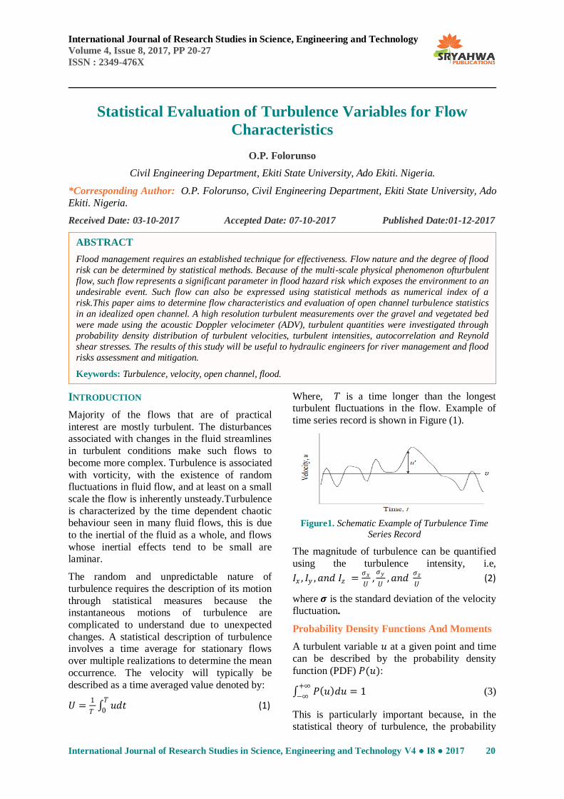
Where, 𝑇 is a time longer than the longest turbulent fluctuations in the flow. Example of

time series record is shown in Figure (1).

Figure1. Schematic Example of Turbulence Time

Series Record

The magnitude of turbulence can be quantified

using the turbulence intensity, i.e,

𝐼𝑥 , 𝐼𝑦 ,𝑎𝑛𝑑 𝐼𝑧 =𝜎𝑥

𝑈,𝜎𝑦

𝑈,𝑎𝑛𝑑

𝜎𝑧

𝑈 (2)

where 𝝈 is the standard deviation of the velocity

fluctuation.

Probability Density Functions And Moments

A turbulent variable 𝑢 at a given point and time

can be described by the probability density

function (PDF) 𝑃(𝑢):

𝑃 𝑢 𝑑𝑢+∞

−∞= 1 (3)

This is particularly important because, in the statistical theory of turbulence, the probability

ABSTRACT

Flood management requires an established technique for effectiveness. Flow nature and the degree of flood

risk can be determined by statistical methods. Because of the multi-scale physical phenomenon ofturbulent

flow, such flow represents a significant parameter in flood hazard risk which exposes the environment to an

undesirable event. Such flow can also be expressed using statistical methods as numerical index of a

risk.This paper aims to determine flow characteristics and evaluation of open channel turbulence statistics

in an idealized open channel. A high resolution turbulent measurements over the gravel and vegetated bed

were made using the acoustic Doppler velocimeter (ADV), turbulent quantities were investigated through

probability density distribution of turbulent velocities, turbulent intensities, autocorrelation and Reynold

shear stresses. The results of this study will be useful to hydraulic engineers for river management and flood

risks assessment and mitigation.

Keywords: Turbulence, velocity, open channel, flood.

Statistical Evaluation of Turbulence Variables for Flow Characteristics

21 International Journal of Research Studies in Science, Engineering and Technology V4 ● I8 ● 2017

density function provides a complete

probabilistic description that permits the estimation and quantification of turbulent flow

variables, for example, the tails of the 𝑝𝑑𝑓 for

flow variables have been reported to be influenced by the scale of eddy motions (Chu et

al., 1996).

The skewness provides information about the

asymmetry of the PDF given as:

𝑆𝑘𝑒𝑤𝑛𝑒𝑠𝑠 (𝜇3) =𝑢′3

𝑢′2 3/2 (4)

where 𝑢′ = 𝑢 − 𝑈 is the turbulent fluctuating

component.

The kurtosis characterizes the flatness of a PDF and is given by the expression:

𝑘𝑢𝑟𝑡𝑜𝑠𝑖𝑠 (𝜇4) =𝑢′4

𝑢′2 2 (5)

A time series with measurements clustered

around the mean has low kurtosis and a time

series by intermittent extreme events are characterized with high kurtosis.

Autocorrelation

The autocorrelation of a random process describes the correlation between values of the

process at different points in time, as a function

of the two times or of the time difference. It

shows the correlation between the consecutive values of the time series. As a time resolved

characteristics for the velocity components, it

plays a major role in the analysis of the flow structures and especially for determining

temporal and spatial flow scales. It can be

computed by shifting the velocity records by a

time delay τ = ∆𝑡 equal to a multiple of the

measurement interval, for each time delay, the

autocorrelation can be obtained as:

𝑅𝑢𝑢 τ = ∆𝑡 = 𝑢′ 𝑡 𝑢′ (𝑡+ τ)

𝑈2 . 𝑈2 (6)

where 𝑅𝑢𝑢 t is the autocorrelation function, 𝑢′

is the fluctuating part of the velocity, and τ is an

increment of time delay (McConville, 2008).

From the autocorrelation functions, the integral

time scale 𝑇𝑢 can be obtained by evaluating

the area under the autocorrelation function

which is normally stop when the function

crosses the 𝑥-axis. Integrating numerically the

autocorrelation function in Equation (6) to give

integral time scale for streamwise velocity

component as shown in Equation (7):

𝑇𝑢 = 𝑅𝑢𝑢 𝑡 𝑑𝑡𝑡

0 (7)

𝑇𝑢 yields a physical interpretation for

turbulence, i.e., it is an indication of the average temporal scale of turbulent eddies (Lacey and

Roy, 2008). Similarly, an integral length scale is

an important parameter in characterizing the structure of turbulence. It measures the longest

correlation distance between the flow velocities

at two points in the flow field (Hinze, 1975).

This can be obtained from Equation (8) as:

𝐿𝑢 = 𝑈 𝑇𝑢 (8)

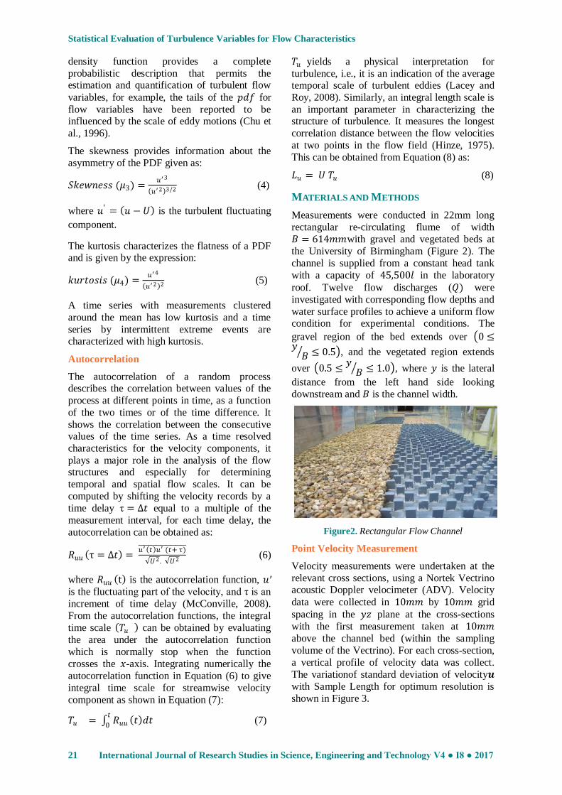
MATERIALS AND METHODS

Measurements were conducted in 22mm long

rectangular re-circulating flume of width

𝐵 = 614𝑚𝑚with gravel and vegetated beds at

the University of Birmingham (Figure 2). The

channel is supplied from a constant head tank

with a capacity of 45,500𝑙 in the laboratory

roof. Twelve flow discharges (𝑄) were

investigated with corresponding flow depths and

water surface profiles to achieve a uniform flow condition for experimental conditions. The

gravel region of the bed extends over 0 ≤𝑦𝐵 ≤ 0.5 , and the vegetated region extends

over 0.5 ≤𝑦𝐵 ≤ 1.0 , where 𝑦 is the lateral

distance from the left hand side looking

downstream and 𝐵 is the channel width.

Figure2. Rectangular Flow Channel

Point Velocity Measurement

Velocity measurements were undertaken at the

relevant cross sections, using a Nortek Vectrino acoustic Doppler velocimeter (ADV). Velocity

data were collected in 10𝑚𝑚 by 10𝑚𝑚 grid

spacing in the 𝑦𝑧 plane at the cross-sections

with the first measurement taken at 10𝑚𝑚

above the channel bed (within the sampling

volume of the Vectrino). For each cross-section,

a vertical profile of velocity data was collect.

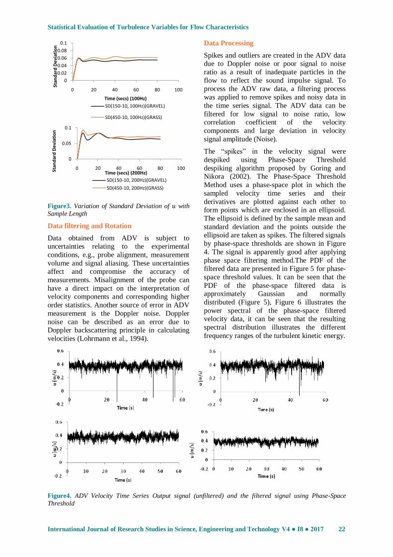
The variationof standard deviation of velocity𝒖

with Sample Length for optimum resolution is

shown in Figure 3.



Figure3. Variation of Standard Deviation of 𝑢 with

Sample Length

Data filtering and Rotation

Data obtained from ADV is subject to uncertainties relating to the experimental

conditions, e.g., probe alignment, measurement

volume and signal aliasing. These uncertainties affect and compromise the accuracy of

measurements. Misalignment of the probe can

have a direct impact on the interpretation of velocity components and corresponding higher

order statistics. Another source of error in ADV

measurement is the Doppler noise. Doppler

noise can be described as an error due to Doppler backscattering principle in calculating

velocities (Lohrmann et al., 1994).

Data Processing

Spikes and outliers are created in the ADV data due to Doppler noise or poor signal to noise

ratio as a result of inadequate particles in the

flow to reflect the sound impulse signal. To process the ADV raw data, a filtering process

was applied to remove spikes and noisy data in

the time series signal. The ADV data can be

filtered for low signal to noise ratio, low correlation coefficient of the velocity

components and large deviation in velocity

signal amplitude (Noise).

The “spikes” in the velocity signal were

despiked using Phase-Space Threshold

despiking algorithm proposed by Goring and Nikora (2002). The Phase-Space Threshold

Method uses a phase-space plot in which the

sampled velocity time series and their

derivatives are plotted against each other to form points which are enclosed in an ellipsoid.

The ellipsoid is defined by the sample mean and

standard deviation and the points outside the ellipsoid are taken as spikes. The filtered signals

by phase-space thresholds are shown in Figure

4. The signal is apparently good after applying

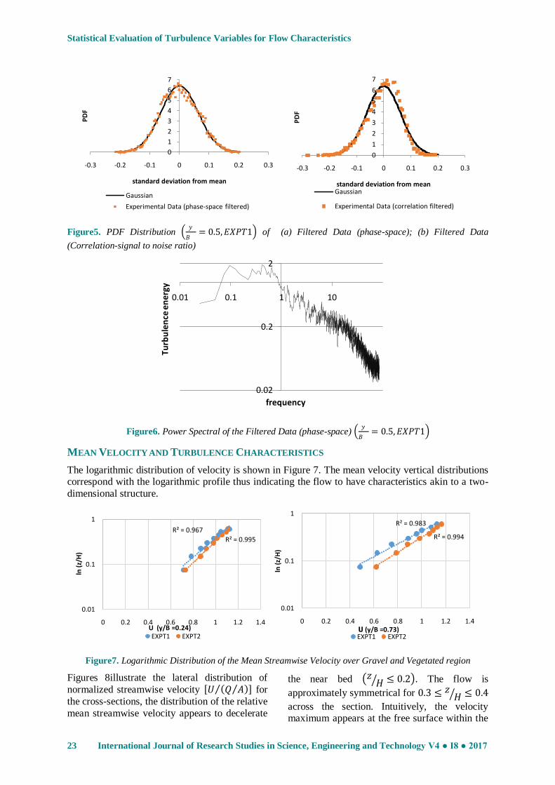
phase space filtering method.The PDF of the filtered data are presented in Figure 5 for phase-

space threshold values. It can be seen that the

PDF of the phase-space filtered data is approximately Gaussian and normally

distributed (Figure 5), Figure 6 illustrates the

power spectral of the phase-space filtered velocity data, it can be seen that the resulting

spectral distribution illustrates the different

frequency ranges of the turbulent kinetic energy.

Figure4. ADV Velocity Time Series Output signal (unfiltered) and the filtered signal using Phase-Space

Threshold

0

0.02

0.04

0.06

0.08

0.1

0 20 40 60 80 100

Stan

dar

d D

evi

atio

n

Time (secs) (100Hz)

SD(150-10, 100Hz)(GRAVEL)

SD(450-10, 100Hz)(GRASS)

0

0.05

0.1

0 20 40 60 80 100Stan

dar

d D

evi

atio

n

Time (secs) (200Hz)

SD(150-10, 200Hz)(GRAVEL)

SD(450-10, 200Hz)(GRASS)



Figure5. PDF Distribution 𝑦

𝐵 = 0.5,𝐸𝑋𝑃𝑇1 of (a) Filtered Data (phase-space); (b) Filtered Data

(Correlation-signal to noise ratio)

Figure6. Power Spectral of the Filtered Data (phase-space) 𝑦

𝐵 = 0.5,𝐸𝑋𝑃𝑇1

MEAN VELOCITY AND TURBULENCE CHARACTERISTICS

The logarithmic distribution of velocity is shown in Figure 7. The mean velocity vertical distributions correspond with the logarithmic profile thus indicating the flow to have characteristics akin to a two-

dimensional structure.

Figure7. Logarithmic Distribution of the Mean Streamwise Velocity over Gravel and Vegetated region

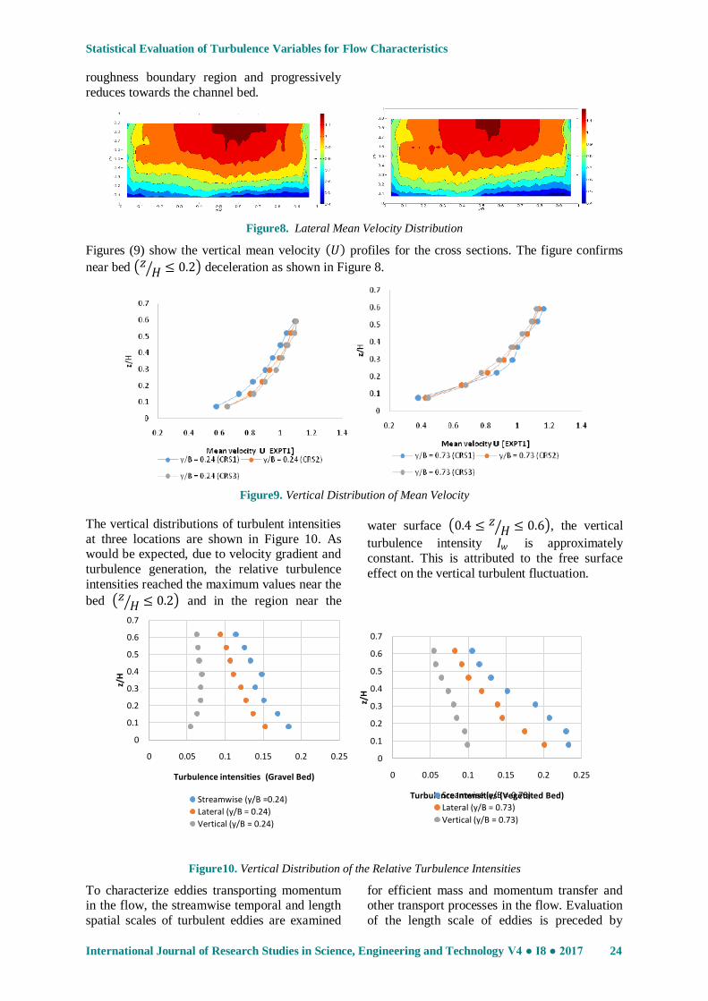
Figures 8illustrate the lateral distribution of

normalized streamwise velocity 𝑈 𝑄 𝐴 for

the cross-sections, the distribution of the relative

mean streamwise velocity appears to decelerate

the near bed 𝑧 𝐻 ≤ 0.2 . The flow is

approximately symmetrical for 0.3 ≤ 𝑧𝐻 ≤ 0.4

across the section. Intuitively, the velocity maximum appears at the free surface within the

0

1

2

3

4

5

6

7

-0.3 -0.2 -0.1 0 0.1 0.2 0.3

PD

F

standard deviation from mean

Gaussian

Experimental Data (phase-space filtered)

0

1

2

3

4

5

6

7

-0.3 -0.2 -0.1 0 0.1 0.2 0.3

PD

F

standard deviation from meanGaussian

Experimental Data (correlation filtered)

0.02

0.2

2

0.01 0.1 1 10

Turb

ule

nce

en

erg

y

frequency

R² = 0.967

R² = 0.995

0.01

0.1

1

0 0.2 0.4 0.6 0.8 1 1.2 1.4

ln (

z/H

)

U (y/B =0.24)EXPT1 EXPT2

R² = 0.983

R² = 0.994

0.01

0.1

1

0 0.2 0.4 0.6 0.8 1 1.2 1.4

ln (

z/H

)

𝗨 (y/B =0.73)EXPT1 EXPT2

a



roughness boundary region and progressively

reduces towards the channel bed.

Figure8. Lateral Mean Velocity Distribution

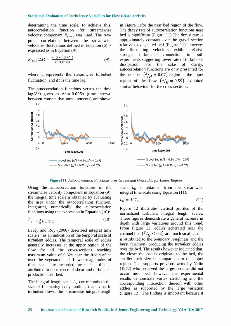
Figures (9) show the vertical mean velocity 𝑈 profiles for the cross sections. The figure confirms

near bed 𝑧 𝐻 ≤ 0.2 deceleration as shown in Figure 8.

Figure9. Vertical Distribution of Mean Velocity

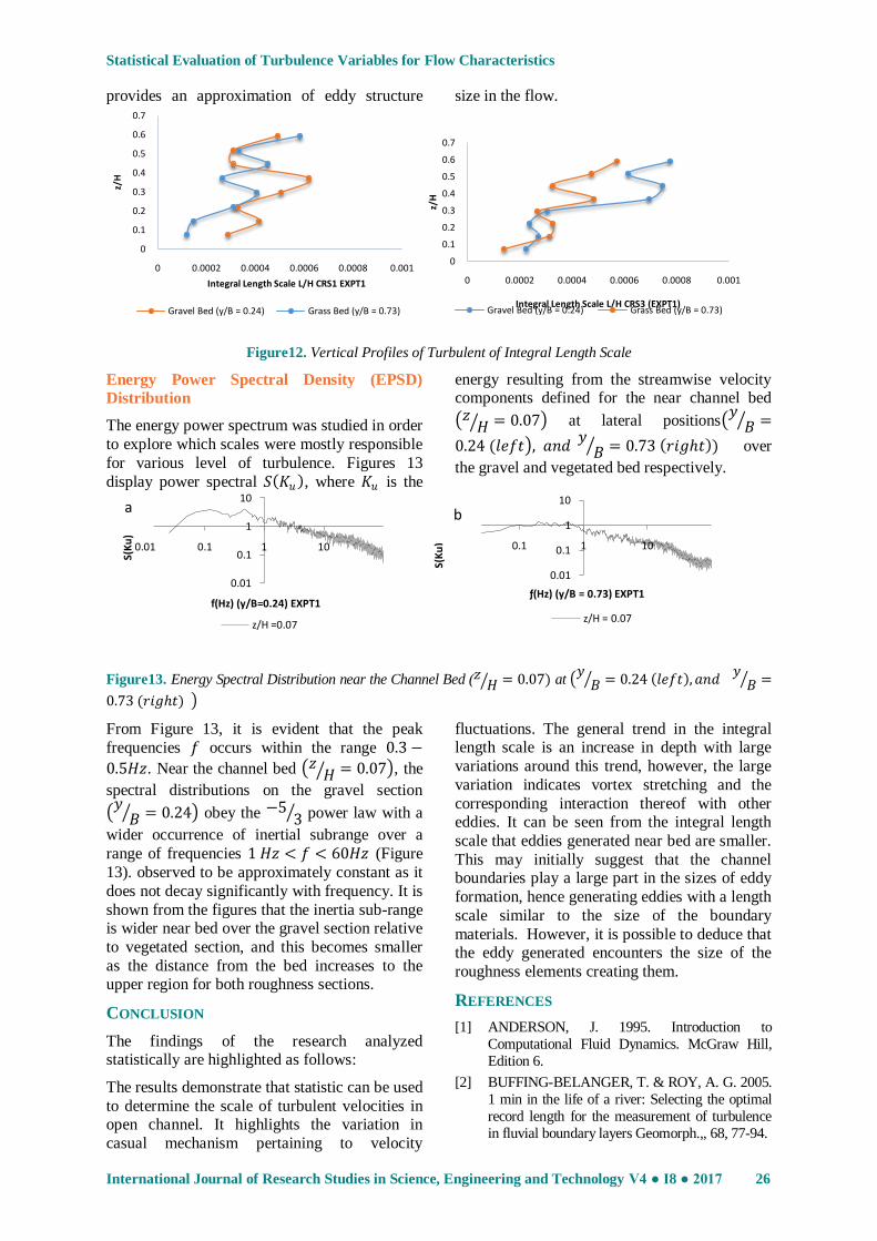
The vertical distributions of turbulent intensities

at three locations are shown in Figure 10. As would be expected, due to velocity gradient and

turbulence generation, the relative turbulence

intensities reached the maximum values near the

bed 𝑧 𝐻 ≤ 0.2 and in the region near the

water surface 0.4 ≤ 𝑧𝐻 ≤ 0.6 , the vertical

turbulence intensity 𝐼𝑤 is approximately

constant. This is attributed to the free surface

effect on the vertical turbulent fluctuation.

Figure10. Vertical Distribution of the Relative Turbulence Intensities

To characterize eddies transporting momentum in the flow, the streamwise temporal and length

spatial scales of turbulent eddies are examined

for efficient mass and momentum transfer and other transport processes in the flow. Evaluation

of the length scale of eddies is preceded by

0

0.1

0.2

0.3

0.4

0.5

0.6

0.7

0 0.05 0.1 0.15 0.2 0.25

z/H

Turbulence intensities (Gravel Bed)

Streamwise (y/B =0.24)

Lateral (y/B = 0.24)

Vertical (y/B = 0.24)

0

0.1

0.2

0.3

0.4

0.5

0.6

0.7

0 0.05 0.1 0.15 0.2 0.25

z/H

Turbulence Intensities (Vegetated Bed)Sreamwise (y/B = 0.73)

Lateral (y/B = 0.73)

Vertical (y/B = 0.73)



determining the time scale, to achieve this,

autocorrelation function for streamewise

velocity component 𝑅(𝑢𝑢 ) was used. The two-

point correlation between the streamwise velocities fluctuations defined in Equation (6) is

expressed as in Equation (9);

𝑅(𝑢𝑢 ) ∆𝑡 = 𝑢 ′ 𝑡 𝑢 ′ 𝑡+∆𝑡

𝑢 ′ 𝑡 𝑢 ′ (𝑡) (9)

where 𝑢′ represents the streamwise turbulent

fluctuation, and ∆𝑡 is the time lag.

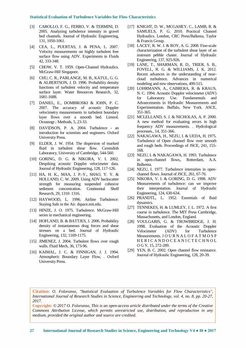
The autocorrelation functions versus the time

lag(∆𝑡) given as ∆𝑡 = 0.005𝑠 (time interval

between consecutive measurements) are shown

in Figure 11for the near bed region of the flow.

The decay rate of autocorrelation functions near bed is significant (Figure 11).The decay rate is

approximately constant over the gravel section

relative to vegetated bed (Figure 11); however the fluctuating velocities exhibit relative

stronger turbulence connection in both

experiments suggesting lower rate of turbulence

dissipation. For the sake of clarity, autocorrelation functions are only presented for

the near bed 𝑧 𝐻 = 0.07 region as the upper

region of the flow 𝑧 𝐻 = 0.59 exhibited

similar behaviour for the cross-sections.

Figure111. Autocorrelation Functions over Gravel and Grass Bed for Lower Region

Using the autocorrelation functions of the streamwise velocity component in Equation (9),

the integral time scale is obtained by evaluating

the area under the autocorrelation function. Integrating numerically the autocorrelation

functions using the expression in Equation (10):

𝑇𝑢 = 𝑅𝑢𝑢 𝑡 𝑑𝑡

𝑡0

(10)

Lacey and Roy (2008) described integral time

scale 𝑇𝑢 as an indication of the temporal scale of turbulent eddies. The temporal scale of eddies

generally increases at the upper region of the

flow for all the cross-sections reaching

maximum value of 0.32s near the free surface over the vegetated bed. Lower magnitudes of

time scale are recorded near bed, this is

attributed to occurrence of shear and turbulence production near bed.

The integral length scale 𝐿𝑢 corresponds to the

size of fluctuating eddy motions that exists in turbulent flows, the streamwise integral length

scale 𝐿𝑢 is obtained from the streamwise integral time scale using Equation (11);

𝐿𝑢 = 𝑈 𝑇𝑢 (11)

Figure 12 illustrates vertical profiles of the

normalized turbulent integral length scales.

These figures demonstrate a general increase in depth with large variations around this trend.

From Figure 12, eddies generated near the

channel bed 𝑧 𝐻 ≤ 0.2 are much smaller, this

is attributed to the boundary roughness and the

burst (ejection) producing the turbulent eddies

over the bed. The results however indicated that, the closer the eddies originate to the bed, the

smaller their size in comparison to the upper

region. This supports previous work by Yalin (1972) who observed the largest eddies did not

occur near bed, however the experimental

results demonstrate vortex stretching and the corresponding interaction thereof with other

eddies as supported by the large variation

(Figure 12). The finding is important because it

-0.4

-0.2

0

0.2

0.4

0.6

0.8

1

1.2

0 500 1000 1500

Co

rre

lati

on

Co

eff

icie

nt

time lag/0.005

Gravel Bed (y/B = 0.24, z/H = 0.07)

Grass Bed (y/B = 0.73, z/H = 0.07)

-0.4

-0.2

0

0.2

0.4

0.6

0.8

1

1.2

0 500 1000corr

ela

tio

n c

oe

ffic

ien

ts

time lag/0.005

Gravel Bed (y/B = 0.24. z/H = 0.07)

Grass Bed (y/B = 0.73, z/H = 0.07)



provides an approximation of eddy structure size in the flow.

Figure12. Vertical Profiles of Turbulent of Integral Length Scale

Energy Power Spectral Density (EPSD)

Distribution

The energy power spectrum was studied in order

to explore which scales were mostly responsible

for various level of turbulence. Figures 13

display power spectral 𝑆 𝐾𝑢 , where 𝐾𝑢 is the

energy resulting from the streamwise velocity components defined for the near channel bed

𝑧 𝐻 = 0.07 at lateral positions 𝑦𝐵 =

0.24 (𝑙𝑒𝑓𝑡 , 𝑎𝑛𝑑 𝑦𝐵 = 0.73 𝑟𝑖𝑔𝑕𝑡 ) over

the gravel and vegetated bed respectively.

Figure13. Energy Spectral Distribution near the Channel Bed (𝑧 𝐻 = 0.07) at 𝑦𝐵 = 0.24 𝑙𝑒𝑓𝑡 ,𝑎𝑛𝑑

𝑦𝐵 =

0.73 (𝑟𝑖𝑔𝑕𝑡)

From Figure 13, it is evident that the peak

frequencies 𝑓 occurs within the range 0.3 −

0.5𝐻𝑧. Near the channel bed 𝑧 𝐻 = 0.07 , the

spectral distributions on the gravel section

𝑦𝐵 = 0.24 obey the −5

3 power law with a

wider occurrence of inertial subrange over a

range of frequencies 1 𝐻𝑧 < 𝑓 < 60𝐻𝑧 (Figure

13). observed to be approximately constant as it

does not decay significantly with frequency. It is

shown from the figures that the inertia sub-range is wider near bed over the gravel section relative

to vegetated section, and this becomes smaller

as the distance from the bed increases to the upper region for both roughness sections.

CONCLUSION

The findings of the research analyzed statistically are highlighted as follows:

The results demonstrate that statistic can be used

to determine the scale of turbulent velocities in open channel. It highlights the variation in

casual mechanism pertaining to velocity

fluctuations. The general trend in the integral length scale is an increase in depth with large

variations around this trend, however, the large

variation indicates vortex stretching and the

corresponding interaction thereof with other eddies. It can be seen from the integral length

scale that eddies generated near bed are smaller.

This may initially suggest that the channel boundaries play a large part in the sizes of eddy

formation, hence generating eddies with a length

scale similar to the size of the boundary

materials. However, it is possible to deduce that the eddy generated encounters the size of the

roughness elements creating them.

REFERENCES

[1] ANDERSON, J. 1995. Introduction to

Computational Fluid Dynamics. McGraw Hill,

Edition 6.

[2] BUFFING-BELANGER, T. & ROY, A. G. 2005.

1 min in the life of a river: Selecting the optimal

record length for the measurement of turbulence

in fluvial boundary layers Geomorph.,, 68, 77-94.

0

0.1

0.2

0.3

0.4

0.5

0.6

0.7

0 0.0002 0.0004 0.0006 0.0008 0.001

z/H

Integral Length Scale L/H CRS1 EXPT1

Gravel Bed (y/B = 0.24) Grass Bed (y/B = 0.73)

0

0.1

0.2

0.3

0.4

0.5

0.6

0.7

0 0.0002 0.0004 0.0006 0.0008 0.001

z/H

Integral Length Scale L/H CRS3 (EXPT1)Gravel Bed (y/B = 0.24) Grass Bed (y/B = 0.73)

0.01

0.1

1

10

0.01 0.1 1 10

S(K

u)

f(Hz) (y/B=0.24) EXPT1

z/H =0.07

0.01

0.1

1

10

0.01 0.1 1 10

S(K

u)

ƒ(Hz) (y/B = 0.73) EXPT1

z/H = 0.07

a b



[3] CAROLLO, F. G., FERRO, V. & TERMINI, D.

2005. Analyzing turbulence intensity in gravel

bed channels. Journal of Hydraulic Engineering,

131, 1050-1061.

[4] CEA, L., PUERTAS, J. & PENA, L. 2007.

Velocity measurements on highly turbulent free

surface flow using ADV. Experiments in Fluids

42, 333-348.

[5] CHOW, V. T. 1959. Open-Channel Hydraulics.

McGraw-Hill Singapore.

[6] CHU, C. R., PARLANGE, M. B., KATUL, G. G. & ALBERTSON, J. D. 1996. Probability density

functions of turbulent velocity and temperature

surface layer. Water Resources Research, 32,

1681-1688.

[7] DANIEL, E., DOMBROSKI & JOHN, P. C.

2007. The accuracy of acoustic Doppler velocimetry measurements in turbulent boundary

layer flows over a smooth bed. Limnol.

Oceanogr.: Methods, 5, 23-33.

[8] DAVIDSON, P. A. 2004. Turbulence - an

introduction for scientists and engineers. Oxford University Press.

[9] ELDER, J. W. 1954. The dispersion of marked

fluid in turbulent shear flow. Cavendish

Laboratory, University of Cambridge, 544-560.

[10] GORING, D. G. & NIKORA, V. I. 2002.

Despiking acoustic Doppler velocimeter data.

Journal of Hydraulic Engineering, 128, 117-126.

[11] HA, H. K., MAA, J. P.-Y., SHAO, Y. Y. &

HOLLAND, C. W. 2009. Using ADV backscatter

strength for measuring suspended cohesive

sediment concentration. Continental Shelf

Research, 29, 1310–1316.

[12] HAYWOOD, L. 1996. Airline Turbulence:

Staying Safe in the Air. dspace.mit.edu.

[13] HINZE, J. O. 1975. Turbulence. McGraw-Hill

series in mechanical engineering.

[14] HOFLAND, B. & BATTJES, J. 2006. Probability

density of instantaneous drag forces and shear

stresses on a bed. Journal of Hydraulic

Engineering, 132, 1169-1175.

[15] JIMENEZ, J. 2004. Turbulent flows over rough

walls. Fluid Mech, 36, 173-96.

[16] KAIMAL, J. C. & FINNIGAN, J. J. 1994. Atmospheric Boundary Layer Flow, . Oxford

University Press.

[17] KNIGHT, D. W., MCGAHEY, C., LAMB, R. &

SAMUELS, P. G. 2010. Practical Channel

Hydraulics. London, CRC Press/Balkena, Taylor

& Francis Group.

[18] LACEY, R. W. J. & ROY, A. G. 2008. Fine-scale characterization of the turbulent shear layer of an

instream pebble cluster. Journal of Hydraulic

Engineering, 137, 925-926.

[19] LANE, T., SHARMAN, R. D., TRIER, S. B.,

FOVELL, R. G. & WILLIAMS, J. K. 2012.

Recent advances in the understanding of near-

cloud turbulence. Advances in numerical

modeling and new observations, 499-515.

[20] LOHRMANN, A., CABRERA, R. & KRAUS,

N. C. 1994. Acoustic Doppler velocimeter (ADV)

for Laboratory Use. Fundamentals and

Advancements in Hydraulic Measurements and Experimentation. Buffalo, New York. ASCE,

351-365.

[21] MCLELLAND, S. J. & NICHOLAS, A. P. 2000.

A new method for evaluating errors in high

frequency ADV measurements. . Hydrological

processes., 14, 351-366.

[22] NAKAGAWA, H., NEZU, I. & UEDA, H. 1975.

Turbulence of Open channel flow over smooth

and rough beds. Proceedings of JSCE, 241, 155-

168.

[23] NEZU, I. & NAKAGAWA, H. 1993. Turbulence in open-channel flows,. Rotterdam, A.A.

Balkema.

[24] NEZU, I. 1977. Turbulence intensities in open-

channel flows. Journal of JSCE, 261, 67-76.

[25] NIKORA, V. I. & GORING, D. G. 1998. ADV

Measurements of turbulence: can we improve

their interpretation. Journal of Hydraulic

Engineering, 124, 630-634.

[26] PRANDTL, L. 1952. Essentials of fluid

dynamics.

[27] TENNEKES, H. & LUMLEY, J. L. 1972. A first

course in turbulence. The MIT Press Cambridge, Massachusetts, and London, England.

[28] VOULGARIS, G. & TROWBRIDGE, J. H.

1998. Evaluation of the Acoustic Doppler

Velocimeter (ADV) for Turbulence

Measurements. J O U R N A L O F A T M O S P

H E R I C A N D O C E A N I C T E C H N O L

O G Y, 15, 272-289.

[29] YEN, B. C. 2002. Open channel flow resistance.

Journal of Hydraulic Engineering, 128, 20-39.

Citation: O. Folorunso, "Statistical Evaluation of Turbulence Variables for Flow Characteristics",

International Journal of Research Studies in Science, Engineering and Technology, vol. 4, no. 8, pp. 20-27, 2017.

Copyright: © 2017 O. Folorunso, This is an open-access article distributed under the terms of the Creative

Commons Attribution License, which permits unrestricted use, distribution, and reproduction in any

medium, provided the original author and source are credited.

Documents

Statistical Evaluation of Turbulence Variables for Flow Characteristicsijrsset.org/pdfs/v4-i8/3.pdf · · 2017-12-01risk.This paper aims to determine flow characteristics and evaluation