Statistical Applications in Genetics and Molecular Biologyyekutiel/eBayes/smyth_2004.pdf · Volume 3, Issue 1 2004 Article 3 Statistical Applications in Genetics and Molecular Biology

Volume 3, Issue 1 2004 Article 3

Statistical Applications in Geneticsand Molecular Biology

Linear Models and Empirical Bayes Methodsfor Assessing Differential Expression in

Microarray Experiments

Gordon K. Smyth, Walter and Eliza Hall Institute

Recommended Citation:Smyth, Gordon K. (2004) "Linear Models and Empirical Bayes Methods for AssessingDifferential Expression in Microarray Experiments," Statistical Applications in Genetics andMolecular Biology: Vol. 3: Iss. 1, Article 3.DOI: 10.2202/1544-6115.1027Available at: http://www.bepress.com/sagmb/vol3/iss1/art3

©2004 by the authors. All rights reserved. No part of this publication may be reproduced, storedin a retrieval system, or transmitted, in any form or by any means, electronic, mechanical,photocopying, recording, or otherwise, without the prior written permission of the publisher,bepress, which has been given certain exclusive rights by the author. Statistical Applications inGenetics and Molecular Biology is produced by Berkeley Electronic Press (bepress).

Linear Models and Empirical Bayes Methodsfor Assessing Differential Expression in

Microarray ExperimentsGordon K. Smyth

Abstract

The problem of identifying differentially expressed genes in designed microarrayexperiments is considered. Lonnstedt and Speed (2002) derived an expression for the posteriorodds of differential expression in a replicated two-color experiment using a simple hierarchicalparametric model. The purpose of this paper is to develop the hierarchical model of Lonnstedt andSpeed (2002) into a practical approach for general microarray experiments with arbitrary numbersof treatments and RNA samples. The model is reset in the context of general linear models witharbitrary coefficients and contrasts of interest. The approach applies equally well to both singlechannel and two color microarray experiments. Consistent, closed form estimators are derived forthe hyperparameters in the model. The estimators proposed have robust behavior even for smallnumbers of arrays and allow for incomplete data arising from spot filtering or spot qualityweights. The posterior odds statistic is reformulated in terms of a moderated t-statistic in whichposterior residual standard deviations are used in place of ordinary standard deviations. Theempirical Bayes approach is equivalent to shrinkage of the estimated sample variances towards apooled estimate, resulting in far more stable inference when the number of arrays is small. The useof moderated t-statistics has the advantage over the posterior odds that the number ofhyperparameters which need to estimated is reduced; in particular, knowledge of the non-null priorfor the fold changes are not required. The moderated t-statistic is shown to follow a t-distributionwith augmented degrees of freedom. The moderated t inferential approach extends toaccommodate tests of composite null hypotheses through the use of moderated F-statistics. Theperformance of the methods is demonstrated in a simulation study. Results are presented for twopublicly available data sets.

KEYWORDS: microarrays, empirical Bayes, linear models, hyperparameters, differentialexpression

Author Notes: Walter and Eliza Hall Institute, 1G Royal Parade, Melbourne 3050, Australia,[email protected]

Erratum

The following information was added January 15, 2009:

In Section 3, the posterior variance s2g is introduced as the posterior

mean of σ2g given s2

g. In fact, s−2g is the posterior mean of σ−2

g .

In Section 4, the second displayed equation should be

p(f) =aν2/2bν1/2f ν1/2−1

B(ν1/2, ν2/2)(a+ bf)ν1/2+ν2/2.

In Section 6.2, all occurrences of n in equations should be G. Thesymbol e refers to the mean of the eg over all G genes.

The following information was added July 1, 2009:

In Section 5, the limit of the odds ratio for d0 + dg large should be

Ogj =pj

1− pj

(vgj

vgj + v0j

)1/2

exp

(t2gj2

v0j

vgj + v0j

).

This replaces the third displayed equation of the section.

1 Introduction

Microarrays are a technology for comparing the expression profiles of genes on a genomicscale across two or more RNA samples. Recent reviews of microarray data analysisinclude the Nature Genetics supplement (2003), Smyth et al (2003), Parmigiani etal (2003) and Speed (2003). This paper considers the problem of identifying geneswhich are differentially expressed across specified conditions in designed microarrayexperiments. This is a massive multiple testing problem in which one or more testsare conducted for each of tens of thousands of genes. The problem is complicated bythe fact that the measured expression levels are often non-normally distributed andhave non-identical and dependent distributions between genes. This paper addressesparticularly the fact that the variability of the expression values differs between genes.

It is well established that allowance needs to be made in the analysis of microarrayexperiments for the amount of multiple testing, perhaps by controlling the familywiseerror rate or the false discovery rate, even though this reduces the power availableto detect changes in expression for individual genes (Ge et al, 2002). On the otherhand, the parallel nature of the inference in microarrays allows some compensatingpossibilities for borrowing information from the ensemble of genes which can assist ininference about each gene individually. One way that this can be done is through theapplication of Bayes or empirical Bayes methods (Efron, 2001, 2003). Efron et al (2001)used a non-parametric empirical Bayes approach for the analysis of factorial data withhigh density oligonucleotide microarray data. This approach has much potential but canbe difficult to apply in practical situations especially by less experienced practitioners.Lonnstedt and Speed (2002), considering replicated two-color microarray experiments,took instead a parametric empirical Bayes approach using a simple mixture of normalmodels and a conjugate prior and derived a pleasingly simple expression for the posteriorodds of differential expression for each gene. The posterior odds expression has provedto be a useful means of ranking genes in terms of evidence for differential expression.

The purpose of this paper is to develop the hierarchical model of Lonnstedt andSpeed (2002) into a practical approach for general microarray experiments with arbi-trary numbers of treatments and RNA samples. The first step is to reset it in thecontext of general linear models with arbitrary coefficients and contrasts of interest.The approach applies to both single channel and two color microarrays. All of thecommonly used microarray platforms such as cDNA, long-oligos and Affymetrix aretherefore accommodated. The second step is to derive consistent, closed form estima-tors for the hyperparameters using the marginal distributions of the observed statistics.The estimators proposed here have robust behavior even for small numbers of arrays andallow for incomplete data arising from spot filtering or spot quality weights. The thirdstep is to reformulate the posterior odds statistic in terms of a moderated t-statisticin which posterior residual standard deviations are used in place of ordinary standarddeviations. This approach makes explicit what was implicit in Lonnstedt and Speed(2002), that the hierarchical model results in a shrinkage of the gene-wise residual sam-ple variances towards a common value, resulting in far more stable inference when thenumber of arrays is small. The use of moderated t-statistic has the advantage over

1

Smyth: Empirical Bayes Methods for Differential Expression

Published by The Berkeley Electronic Press, 2004

the posterior odds of reducing the number of hyperparameters which need to estimatedunder the hierarchical model; in particular, knowledge of the non-null prior for the foldchanges are not required. The moderated t-statistic is shown to follow a t-distributionwith augmented degrees of freedom. The moderated t inferential approach extendsto accommodate tests involving two or more contrasts through the use of moderatedF -statistics.

The idea of using a t-statistic with a Bayesian adjusted denominator was also pro-posed by Baldi and Long (2001) who developed the useful cyberT program. Their workwas limited though to two-sample control versus treatment designs and their model didnot distinguish between differentially and non-differentially expressed genes. They alsodid not develop consistent estimators for the hyperparameters. The degrees of freedomassociated with the prior distribution of the variances was set to a default value whilethe prior variance was simply equated to locally pooled sample variances.

Tusher et al (2001), Efron et al (2001) and Broberg (2003) have used t statisticswith offset standard deviations. This is similar in principle to the moderated t-statisticsused here but the offset t-statistics are not motivated by a model and do not have anassociated distributional theory. Tusher et al (2001) estimated the offset by minimizinga coefficient of variation while Efron et al (2001) used a percentile of the distributionof sample standard deviations. Broberg (2003) considered the two sample problem andproposed a computationally intensive method of determining the offset by minimizing acombination of estimated false positive and false negative rates over a grid of significancelevels and offsets. Cui and Churchill (2003) give a review of test statistics for differentialexpression for microarray experiments.

Newton et al (2001), Newton and Kendziorski (2003) and Kendziorski et al (2003)have considered empirical Bayes models for expression based on gamma and log-normaldistributions. Other authors have used Bayesian methods for other purposes in mi-croarray data analysis. Ibrahim et al (2002) for example propose Bayesian models withcorrelated priors to model gene expression and to classify between normal and tumortissues.

Other approaches to linear models for microarray data analysis have been describedby Kerr et al (2000), Jin et al (2001), Wolfinger et al (2001), Chu et al (2002), Yangand Speed (2003) and Lonnstedt et al (2003). Kerr et al (2000) propose a single linearmodel for an entire microarray experiment whereas in this paper a separate linear modelis fitted for each gene. The single linear model approach assumes all equal variancesacross genes whereas the current paper is designed to accommodate different variances.Jin et al (2001) and Wolfinger et al (2001) fit separate models for each gene but modelthe individual channels of two color microarray data requiring the use of mixed linearmodels to accommodate the correlation between observations on the same spot. Chuet al (2002) propose mixed models for single channel oligonucleotide array experimentswith multiple probes per gene. The methods of the current paper assume linear modelswith a single component of variance and so do not apply directly to the mixed modelapproach, although ideas similar to those used here could be developed. Yang andSpeed (2003) and Lonnstedt et al (2003) take an linear modeling approach similar tothat of the current paper.

2

Statistical Applications in Genetics and Molecular Biology, Vol. 3 [2004], Iss. 1, Art. 3

http://www.bepress.com/sagmb/vol3/iss1/art3

A B A B

ARef B

A B

C

(a) (b)

(c) (d)

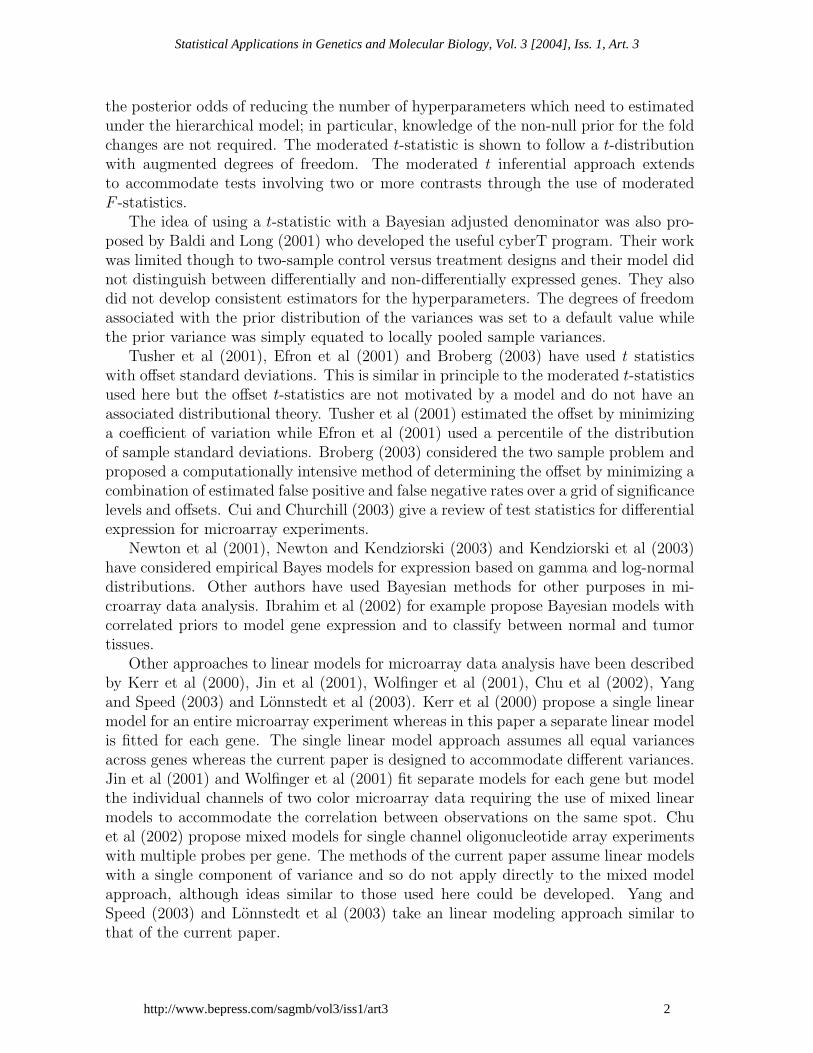
Figure 1: Example designs for two color microarrays.

The plan of this paper is as follows. Section 2 explains the linear modelling approachto the analysis of designed experiments and specifies the response model and distribu-tional assumptions. Section 3 sets out the prior assumptions and defines the posteriorvariances and moderated t-statistics. Section 4 derives marginal distributions under thehierarchical model for the observed statistics. Section 5 derives the posterior odds ofdifferential expression and relates it to the t-statistic. The inferential approach basedon moderated t and F statistics is elaborated in Section 6. Section 7 derives estimatorsfor the hyperparameters. Section 8 compares the estimators with earlier statistics in asimulation study. Section 9 illustrates the methodology on two publicly available datasets. Finally, Section 10 makes some remarks on available software.

2 Linear Models for Microarray Data

This section describes how gene-wise linear models arise from experimental designs andstates the distributional assumptions about the data which will used in the remainderof the paper. The design of any microarray experiment can be represented in terms ofa linear model for each gene. Figure 1 displays some examples of simple designs withtwo-color arrays using arrow notation as in Kerr and Churchill (2001). Each arrowrepresents a microarray. The arrow points towards the RNA sample which is labelledred and the sample at the base of the arrow is labelled green. The symbols A, B and Crepresent RNA sources to be compared. In experiment (a) there is only one microarraywhich compares RNA sample A and B. For this experiment one can only compute thelog-ratios of expression yg = log2(Rg)− log2(Gg) where Rg and Gg are the red and greenintensities for gene g. Design (b) is a dye-swap experiment leading to a very simplelinear model with responses yg1 and yg2 which are log-ratios from the two microarraysand design matrix

X =

(1−1

).

3



The regression coefficient here estimates the contrast B − A on the log-scale, just asfor design (a), but with two arrays there is one degree of freedom for error. Design (c)compares samples A and B indirectly through a common reference RNA sample. Anappropriate design matrix for this experiment is

X =

−1 01 01 1

which produces a linear model in which the first coefficient estimates the differencebetween A and the reference sample while the second estimates the difference of interest,B−A. Design (d) is a simple saturated direct design comparing three samples. Differentdesign matrices can obviously be chosen corresponding to different parametrizations.One choice is

X =

1 00 1

−1 −1

so that the coefficients correspond to the differences B − A and C −B respectively.

Unlike two-color microarrays, single color or high density oligonucleotide microarraysusually yield a single expression value for each gene for each array, i.e., competitivehybridization and two color considerations are absent. For such microarrays, designmatrices can be formed exactly as in classical linear model practice from the biologicalfactors underlying the experimental layout.

In general we assume that we have a set of n microarrays yielding a response vectoryT

g = (yg1, . . . , ygn) for the gth gene. The responses will usually be log-ratios for two-color data or log-intensities for single channel data, although other transformations arepossible. The responses are assumed to be suitably normalized to remove dye-bias andother technological artifacts; see for example Huber et al (2002) or Smyth and Speed(2003). In the case of high density oligonucleotide array, the probes are assumed tohave been normalized to produce an expression summary, represented here as ygi, foreach gene on each array as in Li and Wong (2001) or Irizarry et al (2003). We assumethat

E(yg) = Xαg

where X is a design matrix of full column rank and αg is a coefficient vector. Weassume

var(yg) = Wgσ2g

where Wg is a known non-negative definite weight matrix. The vector yg may containmissing values and the matrix Wg may contain diagonal weights which are zero.

Certain contrasts of the coefficients are assumed to be of biological interest andthese are defined by βg = CT αg. We assume that it is of interest to test whetherindividual contrast values βgj are equal to zero. For example, with design (d) abovethe experimenter might want to make all the pairwise comparisons B − A, C − B and

4



C − A which correspond to the contrast matrix

C =

(1 0 10 1 1

)

There may be more or fewer contrasts than coefficients for the linear model, althoughif more then the contrasts will be linearly dependent. As another example, considera simple time course experiment with two single-channel microarrays hybridized withRNA taken at each of the times 0, 1 and 2. If the numbering of the arrays correspondsto time order then we might choose

X =

1 0 01 0 00 1 00 1 00 0 10 0 1

so that αgj represents the expression level at the jth time, and

C =

−1 01 −10 1

so that the contrasts measure the change from time 0 to time 1 and from time 1 totime 2 respectively. For an experiment such as this it will most likely be of interest totest the hypotheses βg1 = 0 and βg2 = 0 simultaneously as well as individually becausegenes with βg1 = βg2 = 0 are those which do not change over time. Composite nullhypotheses are addressed in Section 7.

We assume that the linear model is fitted to the responses for each gene to obtaincoefficient estimators αg, estimators s2

g of σ2g and estimated covariance matrices

var(αg) = Vgs2g

where Vg is a positive definite matrix not depending on s2g. The contrast estimators are

βg = CT αg with estimated covariance matrices

var(βg) = CTVgCs2g.

The responses yg are not necessarily assumed to be normal and the fitting of the linearmodel is not assumed to be by least squares. However the contrast estimators areassumed to be approximately normal with mean βg and covariance matrix CTVgCσ

2g

and the residual variances s2g are assumed to follow approximately a scaled chisquare

distribution. The unscaled covariance matrix Vg may depend on αg, for example ifrobust regression is used to fit the linear model. If so, the covariance matrix is assumed

5



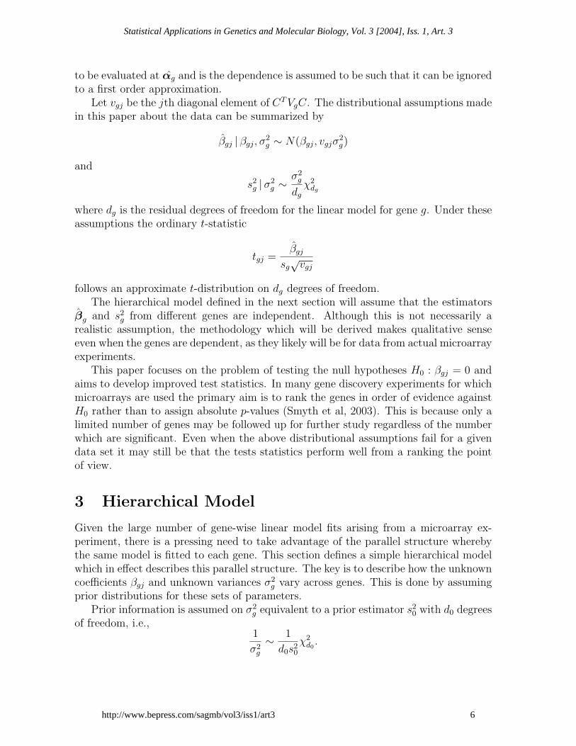
to be evaluated at αg and is the dependence is assumed to be such that it can be ignoredto a first order approximation.

Let vgj be the jth diagonal element of CTVgC. The distributional assumptions madein this paper about the data can be summarized by

βgj | βgj, σ2g ∼ N(βgj, vgjσ

2g)

and

s2g |σ2

g ∼σ2

g

dg

χ2dg

where dg is the residual degrees of freedom for the linear model for gene g. Under theseassumptions the ordinary t-statistic

tgj =βgj

sg√vgj

follows an approximate t-distribution on dg degrees of freedom.The hierarchical model defined in the next section will assume that the estimators

βg and s2g from different genes are independent. Although this is not necessarily a

realistic assumption, the methodology which will be derived makes qualitative senseeven when the genes are dependent, as they likely will be for data from actual microarrayexperiments.

This paper focuses on the problem of testing the null hypotheses H0 : βgj = 0 andaims to develop improved test statistics. In many gene discovery experiments for whichmicroarrays are used the primary aim is to rank the genes in order of evidence againstH0 rather than to assign absolute p-values (Smyth et al, 2003). This is because only alimited number of genes may be followed up for further study regardless of the numberwhich are significant. Even when the above distributional assumptions fail for a givendata set it may still be that the tests statistics perform well from a ranking the pointof view.

3 Hierarchical Model

Given the large number of gene-wise linear model fits arising from a microarray ex-periment, there is a pressing need to take advantage of the parallel structure wherebythe same model is fitted to each gene. This section defines a simple hierarchical modelwhich in effect describes this parallel structure. The key is to describe how the unknowncoefficients βgj and unknown variances σ2

g vary across genes. This is done by assumingprior distributions for these sets of parameters.

Prior information is assumed on σ2g equivalent to a prior estimator s2

0 with d0 degreesof freedom, i.e.,

1

σ2g

∼ 1

d0s20

χ2d0.

6



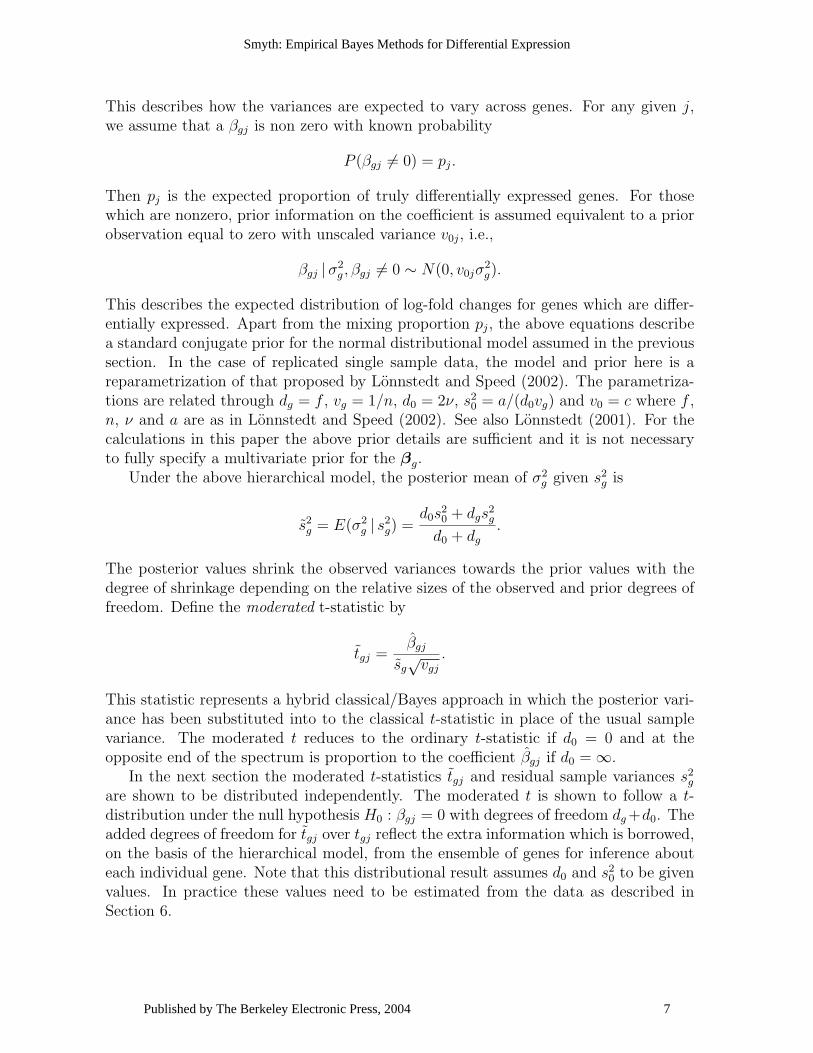
This describes how the variances are expected to vary across genes. For any given j,we assume that a βgj is non zero with known probability

P (βgj 6= 0) = pj.

Then pj is the expected proportion of truly differentially expressed genes. For thosewhich are nonzero, prior information on the coefficient is assumed equivalent to a priorobservation equal to zero with unscaled variance v0j, i.e.,

βgj |σ2g , βgj 6= 0 ∼ N(0, v0jσ

2g).

This describes the expected distribution of log-fold changes for genes which are differ-entially expressed. Apart from the mixing proportion pj, the above equations describea standard conjugate prior for the normal distributional model assumed in the previoussection. In the case of replicated single sample data, the model and prior here is areparametrization of that proposed by Lonnstedt and Speed (2002). The parametriza-tions are related through dg = f , vg = 1/n, d0 = 2ν, s2

0 = a/(d0vg) and v0 = c where f ,n, ν and a are as in Lonnstedt and Speed (2002). See also Lonnstedt (2001). For thecalculations in this paper the above prior details are sufficient and it is not necessaryto fully specify a multivariate prior for the βg.

Under the above hierarchical model, the posterior mean of σ2g given s2

g is

s2g = E(σ2

g | s2g) =

d0s20 + dgs

2g

d0 + dg

.

The posterior values shrink the observed variances towards the prior values with thedegree of shrinkage depending on the relative sizes of the observed and prior degrees offreedom. Define the moderated t-statistic by

tgj =βgj

sg√vgj

.

This statistic represents a hybrid classical/Bayes approach in which the posterior vari-ance has been substituted into to the classical t-statistic in place of the usual samplevariance. The moderated t reduces to the ordinary t-statistic if d0 = 0 and at theopposite end of the spectrum is proportion to the coefficient βgj if d0 = ∞.

In the next section the moderated t-statistics tgj and residual sample variances s2g

are shown to be distributed independently. The moderated t is shown to follow a t-distribution under the null hypothesis H0 : βgj = 0 with degrees of freedom dg +d0. Theadded degrees of freedom for tgj over tgj reflect the extra information which is borrowed,on the basis of the hierarchical model, from the ensemble of genes for inference abouteach individual gene. Note that this distributional result assumes d0 and s2

0 to be givenvalues. In practice these values need to be estimated from the data as described inSection 6.

7



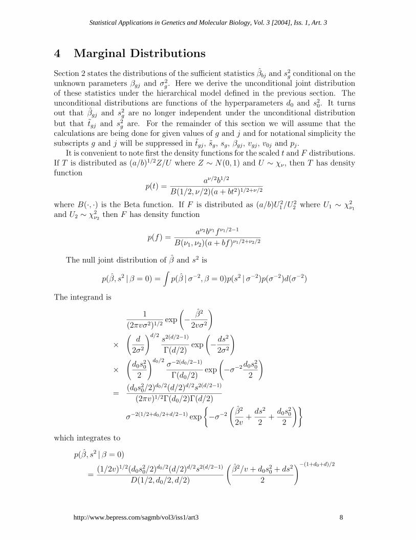
4 Marginal Distributions

Section 2 states the distributions of the sufficient statistics βbj and s2g conditional on the

unknown parameters βgj and σ2g . Here we derive the unconditional joint distribution

of these statistics under the hierarchical model defined in the previous section. Theunconditional distributions are functions of the hyperparameters d0 and s2

0. It turnsout that βgj and s2

g are no longer independent under the unconditional distribution

but that tgj and s2g are. For the remainder of this section we will assume that the

calculations are being done for given values of g and j and for notational simplicity thesubscripts g and j will be suppressed in tgj, sg, sg, βgj, vgj, v0j and pj.

It is convenient to note first the density functions for the scaled t and F distributions.If T is distributed as (a/b)1/2Z/U where Z ∼ N(0, 1) and U ∼ χν , then T has densityfunction

p(t) =aν/2b1/2

B(1/2, ν/2)(a+ bt2)1/2+ν/2

where B(·, ·) is the Beta function. If F is distributed as (a/b)U21/U

22 where U1 ∼ χ2

ν1

and U2 ∼ χ2ν2

then F has density function

p(f) =aν2bν1f ν1/2−1

B(ν1, ν2)(a+ bf)ν1/2+ν2/2

The null joint distribution of β and s2 is

p(β, s2 | β = 0) =∫p(β |σ−2, β = 0)p(s2 |σ−2)p(σ−2)d(σ−2)

The integrand is

1

(2πvσ2)1/2exp

(− β2

2vσ2

)

×(d

2σ2

)d/2s2(d/2−1)

Γ(d/2)exp

(− ds

2

2σ2

)

×(d0s

20

2

)d0/2σ−2(d0/2−1)

Γ(d0/2)exp

(−σ−2d0s

20

2

)

=(d0s

20/2)d0/2(d/2)d/2s2(d/2−1)

(2πv)1/2Γ(d0/2)Γ(d/2)

σ−2(1/2+d0/2+d/2−1) exp

{−σ−2

(β2

2v+ds2

2+d0s

20

2

)}

which integrates to

p(β, s2 | β = 0)

=(1/2v)1/2(d0s

20/2)d0/2(d/2)d/2s2(d/2−1)

D(1/2, d0/2, d/2)

(β2/v + d0s

20 + ds2

2

)−(1+d0+d)/2

8



where D() is the Dirichlet function.The null joint distribution of t and s2 is

p(t, s2 | β = 0) = sv1/2p(β, s2 | β = 0)

which after collection of factors yields

p(t, s2 | β = 0) =(d0s

20)

d0/2dd/2s2(d/2−1)

B(d/2, d0/2)(d0s20 + ds2)d0/2+d/2

× (d0 + d)−1/2

B(1/2, d0/2 + d/2)

(1 +

t2

d0 + d

)−(1+d0+d)/2

This shows that t and s2 are independent with

s2 ∼ s20Fd,d0

andt | β = 0 ∼ td0+d.

The above derivation goes through similarly with β 6= 0, the only difference being that

t | β 6= 0 ∼ (1 + v0/v)1/2 td0+d.

The marginal distribution of t over all the genes is therefore a mixture of a scaledt-distribution and an ordinary t-distribution with mixing proportions p and 1 − p re-spectively.

5 Posterior Odds

Given the unconditional distribution of tgj and s2g from the previous section, it is now

easy to compute the posterior odds than any particular gene g is differentially expressedwith respect to contrast βgj. The odds that the gth gene has non-zero βgj is

Ogj =p(βgj 6= 0 | tgj, s

2g)

p(βgj = 0 | tgj, s2g)

=p(βgj 6= 0, tgj, s

2g)

p(βgj = 0, tgj, s2g)

=pj

1− pj

p(tgj | βgj 6= 0)

p(tgj | βgj = 0)

since tgj and s2g are independent and the distribution of s2

g does not depend on βgj.

Substituting the density for tgj from Section 4 gives

Ogj =pj

1− pj

(vgj

vgj + v0j

)1/2 t2gj + d0 + dg

t2gjvgj

vgj+v0j+ d0 + dg

(1+d0+dg)/2

This agrees with equation (7) of Lonnstedt and Speed (2002). In the limit for d0 + dg

large, the odds ratio reduces to

Ogj =pj

1− pj

(vgj

vgj + v0j

)1/2

exp

(t2gj

2

vgj

vgj + v0j

).

9



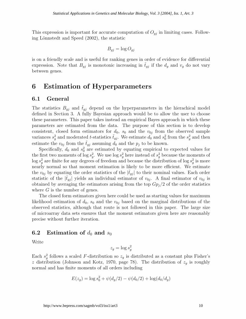
This expression is important for accurate computation of Ogj in limiting cases. Follow-ing Lonnstedt and Speed (2002), the statistic

Bgj = logOgj

is on a friendly scale and is useful for ranking genes in order of evidence for differentialexpression. Note that Bgj is monotonic increasing in tgj if the dg and vg do not varybetween genes.

6 Estimation of Hyperparameters

6.1 General

The statistics Bgj and tgj depend on the hyperparameters in the hierachical modeldefined in Section 3. A fully Bayesian approach would be to allow the user to choosethese parameters. This paper takes instead an empirical Bayes approach in which theseparameters are estimated from the data. The purpose of this section is to developconsistent, closed form estimators for d0, s0 and the v0j from the observed samplevariances s2

g and moderated t-statistics tgj. We estimate d0 and s20 from the s2

g and then

estimate the v0j from the tgj assuming d0 and the pj to be known.Specifically, d0 and s2

0 are estimated by equating empirical to expected values forthe first two moments of log s2

g. We use log s2g here instead of s2

g because the moments oflog s2

g are finite for any degrees of freedom and because the distribution of log s2g is more

nearly normal so that moment estimation is likely to be more efficient. We estimatethe v0j by equating the order statistics of the |tgj| to their nominal values. Each orderstatistic of the |tgj| yields an individual estimator of v0j. A final estimator of v0j isobtained by averaging the estimators arising from the top Gpj/2 of the order statisticswhere G is the number of genes.

The closed form estimators given here could be used as starting values for maximumlikelihood estimation of d0, s0 and the v0j based on the marginal distributions of theobserved statistics, although that route is not followed in this paper. The large sizeof microarray data sets ensures that the moment estimators given here are reasonablyprecise without further iteration.

6.2 Estimation of d0 and s0

Writezg = log s2

g

Each s2g follows a scaled F -distribution so zg is distributed as a constant plus Fisher’s

z distribution (Johnson and Kotz, 1970, page 78). The distribution of zg is roughlynormal and has finite moments of all orders including

E(zg) = log s20 + ψ(dg/2)− ψ(d0/2) + log(d0/dg)

10



andvar(zg) = ψ′(dg/2) + ψ′(d0/2)

where ψ() and ψ′() are the digamma and trigamma functions respectively. Write

eg = zg − ψ(dg/2) + log(dg/2)

ThenE(eg) = log s2

0 − ψ(d0/2) + log(d0/2)

andE{(eg − e)2n/(n− 1)− ψ′(dg/2)} ≈ ψ′(d0/2)

We can therefore estimate d0 by solving

ψ′(d0/2) = mean{(eg − e)2n/(n− 1)− ψ′(dg/2)

}(1)

for d0. Although the inverse of the trigamma function is not a standard mathematicalfunction, equation (1) can be solved very efficiently using a monotonically convergentNewton iteration as described in the appendix.

Given an estimate for d0, s20 can be estimated by

s20 = exp {e+ ψ(d0/2)− log(d0/2)}

This estimate for s20 is usually somewhat less than the mean of the s2

g in recognition ofthe skewness of the F -distribution.

Note that these estimators allow for dg to differ between genes and therefore allowfor arbitrary missing values in the expression data. Note also that any gene for whichdg = 0 will receive s2

g = s20.

In the case that mean {(eg − e)2n/(n− 1)− ψ′(dg/2)} ≤ 0, (1) cannot be solvedbecause the variability of the s2

g is less than or equal to that expected from chisquaresampling variability. In that case there is no evidence that the underlying variances σ2

g

vary between genes so d0 is set to positive infinity and s20 = exp(e).

6.3 Estimation of v0j

In this section we consider the estimation of the v0j for a given j. For ease of notation,the subscript j will be omitted from tgj, vgj, v0j and pj for the remainder of this section.

Gene g yields a moderated t-statistic tg. The cumulative distribution function of tgis

F (tg; vg, v0, d0 + dg) = pF

tg{

vg

vg + v0

}1/2

; d0 + dg

+ (1− p)F(tg; d0 + dg

)

where F (·; k) is the cumulative distribution function of the t-distribution on k degreesof freedom. Let r be the rank of gene g when the |tg| are sorted in descending order.

11



We match the p-value of any particular |tg| to its nominal value given its rank. For anyparticular gene g and rank r we need to solve

2F (−|tg|; vg, v0, d0 + dg) =r − 0.5

G(2)

for v0. The left-hand side is the actual p-value given the parameters and the right-handside is the nominal value for the p-value of rank r. The interpretation is that, if aprobability plot was constructed by plotting the |tg| against the theoretical quantilescorresponding to probabilities (r − 0.5)/G, (2) is the condition that a particular valueof |tg| will lie exactly on the line of equality. The value of v0 which solves (2) is

v0 = vg

(t2g

q2target

− 1

)

withqtarget = F−1 (ptarget; d0 + dg)

and

ptarget =1

p

{r − 0.5

2G− (1− p)F (−|tg|; d0 + dg)

}provided that 0 < ptarget < 1 and qtarget ≤ |tg|.

If |tg| lies above the line of equality in a t-distribution probability plot, i.e., ifF (−|tg|; d0 +dg) < (r− 0.5)/(2G), then ptarget > 0 and v0 > 0. Restricting to those val-ues of r for which (r− 0.5)/(2G) < p ensures also that ptarget < 1 so that the estimatorof v0 is defined. If |tg| does not lie above the line of equality then the best estimate forv0 is zero.

To get a combined estimator of v0, we obtain individual estimators of v0 for r =1, . . . , Gp/2 and set v0 to be the mean of these estimators. The combined estimator willbe positive, unless none of the top Gp/2 values for |tg| exceed the corresponding orderstatistics of the t-distribution, in which case the estimator will be zero.

6.4 Practical Considerations: Estimation of pj

In principle it is not difficult to estimate the proportions pj from the data as well asthe other hyperparameters. A natural estimator would be to iteratively set

pj =1

G

G∑i=1

Ogj

1 +Ogj

since Ogj/(1 + Ogj) is the estimated probability that gene g is differentially expressed,and there are other possibilities such as maximum likelihood estimation. The datahowever contain considerably more information about d0 and s2

0 than about the v0j andthe pj. This is because all the genes contribute to estimation of d0 and s2

0 whereas onlythose which are differential expressed contribute to estimation of v0j or pj, and eventhat indirectly as the identity of the differentially expressed genes is unknown.

12



Any set of sample variances s2g leads to useful estimates of d0 and s2

0. On theother hand, the estimation of v0j and pj is somewhat unstable in that estimates on theboundaries pj = 0, pj = 1 or v0j = 0 have positive probability and these boundaryvalues lead to degenerate values for the posterior odds statistics Bgj. Even when not onthe boundary, the estimator for pj is likely to be sensitive to the particular form of theprior distribution assumed for βgj and possibly also to dependence between the genes(Ferkingstad et al, 2003).

A practical strategy to bypass these problems is to set the pj to values chosen by

the user, perhaps pj = 0.01 or some other small value. Since v1/20j σg is the standard

deviation of the log-fold-changes for differentially expressed genes, and because thisstandard deviation cannot be unreasonably small or large in a microarray experiment,it seems reasonable to place some prior bounds on v

1/20j s0 as well. In the software package

Limma which implements the methods in this paper, the user is allowed to place limitson the possible values for v

1/20j s0. By default these limits are set at 0.1 and 4, chosen to

include a wide range of reasonable values. For many data sets these limits do not comeinto play but they do prevent very small or very large estimated values for v0j.

7 Inference Using Moderated t and F Statistics

As already noted, the odds ratio statistic for differential expression derived in Section 5 ismonotonic increasing in |tgj| for any given j if dg and vg do not vary between genes. Thisshows that the moderated t-statistic is an appropriate statistic for assessing differentialexpression and is equivalent to Bgj as a means of ranking genes. Even when dg and vg

do vary, it is likely that p-values from the tgj will rank the genes in very similar orderto the Bgj.

The moderated t has the advantage over the B-statistic that Bgj depends on hy-perparameters v0j and pj for all j as well as d0 and s2

0 whereas tgj depends only on d0

and s20. This means that the moderated t does not require knowledge of the proportion

of differentially expressed genes, a potentially contentious parameter, nor does it makeany assumptions about the magnitude of differential expression when it exists. Themoderated t does require knowledge of d0 and s2

0, which describe the variability of thetrue gene-wise variances, but these hyperparameters can be estimated in stable fashionas described in Section 6.

The moderated t has the advantage over the ordinary t statistic that large statisticsare less likely to arise merely from under-estimated sample variances. This is becausethe posterior variance s2

g offsets the small sample variances heavily in a relative sensewhile larger sample variances are moderated to a lesser relative degree. In this respectthe moderated t statistic is similar in spirit to t-statistics with offset standard deviation.Provided that d0 <∞ and dg > 0, the moderated t-statistic can be written

tgj =

(d0 + dg

dg

)1/2βgj√s2∗,gvgj

13



where s2∗,g = s2

g +(d0/dg)s20. This shows that the moderated t-statistic is proportional to

a t-statistic with sample variances offset by a constant if the dg are equal. Test statisticswith offset standard deviations of the form

t∗,gj =βgj

(sg + a)√vgj

,

where a is a positive constant, have been used by Tusher et al (2001), Efron et al (2001)and Broberg (2003). Note that t∗ offsets the standard deviation while t offsets thevariance so the two statistics are not functions of one another. Unlike the moderatedt, the offset statistic t∗,gj is not connected in any formal way with the posterior odds ofdifferential expression and does not have an associated distributional theory.

The moderated t-statistic tgj may be used for inference about βgj in a similar way tothat in which the ordinary t-statistic would be used, except that the degrees of freedomare dg + d0 instead of dg. The fact that the hyperparameters d0 and s2

0 are estimatedfrom the data does not impact greatly on the individual test statistics because thehyperparameters are estimated using data from all the genes, meaning that they areestimated relatively precisely and can be taken to be known at the individual gene level.

The moderated t-statistics also lead naturally to moderated F -statistics which canbe used to test hypotheses about any set of contrasts simultaneously. Appropriatequadratic forms of moderated t-statistics follow F -distributions just as do quadraticforms of ordinary t-statistics. Suppose that we wish to test all contrasts for a given geneequal to zero, i.e., H0 : βg = 0. The correlation matrix of βg is Rg = U−1

g CTVgCU−1g

where Ug is the diagonal matrix with unscaled standard deviations (vgj)1/2 on the di-

agonal. Let r be the column rank of C. Let Qg be such that QTg RgQg = Ir and let

qg = QTg tg. Then

Fg = qTg qg/r = tT

g QgQTg tg/r ∼ Fr,d0+dg

If we choose the columns of Qg to be the eigenvectors spanning the range space of Rg

then QTg RgQg = Λg is a diagonal matrix and

Fg = qTg Λ−1

g qg/r ∼ Fr,d0+dg .

The statistic Fg is simply the usual F -statistic from linear model theory for testingβg = 0 but with the posterior variance s2

g substituted for the sample variance s2g in the

denominator.

8 Simulation Results

This section presents a simulation study comparing the moderated t-statistic with fourother statistics for ranking genes in terms of evidence for differential expression. Themoderated t statistic is compared with (i) ordinary fold change, equivalent to |βgj|,(ii) the ordinary t-statistic |tgj|, (iii) Efron’s idea of offsetting the standard deviationsby their 90th percentile and (iv) the original Lonnstedt and Speed (2002) method as

14



0 50 100 150 200

050

100

150

N Genes Selected

N F

alse

Dis

cove

ries

Fold ChangeSMAEfron tModerated tOrdinary t

Variances Different

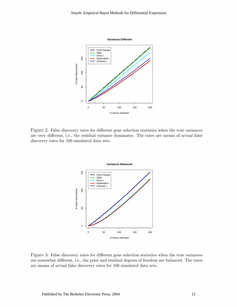
Figure 2: False discovery rates for different gene selection statistics when the true variancesare very different, i.e., the residual variance dominates. The rates are means of actual falsediscovery rates for 100 simulated data sets.

0 50 100 150 200

050

100

150

N Genes Selected

N F

alse

Dis

cove

ries


Variances Balanced

Figure 3: False discovery rates for different gene selection statistics when the true variancesare somewhat different, i.e., the prior and residual degrees of freedom are balanced. The ratesare means of actual false discovery rates for 100 simulated data sets.

15



0 50 100 150 200

050

100

150

N Genes Selected

N F

alse

Dis

cove

ries


Variances Similar

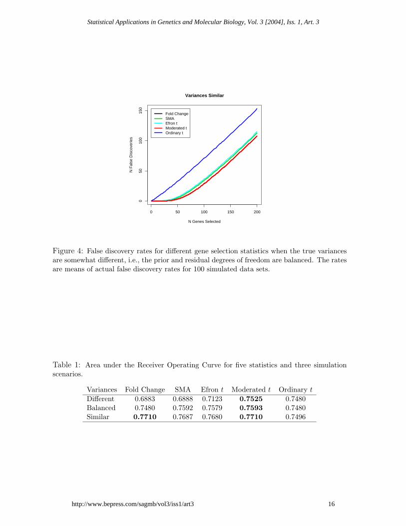
Figure 4: False discovery rates for different gene selection statistics when the true variancesare somewhat different, i.e., the prior and residual degrees of freedom are balanced. The ratesare means of actual false discovery rates for 100 simulated data sets.

Table 1: Area under the Receiver Operating Curve for five statistics and three simulationscenarios.

Variances Fold Change SMA Efron t Moderated t Ordinary t

Different 0.6883 0.6888 0.7123 0.7525 0.7480Balanced 0.7480 0.7592 0.7579 0.7593 0.7480Similar 0.7710 0.7687 0.7680 0.7710 0.7496

16



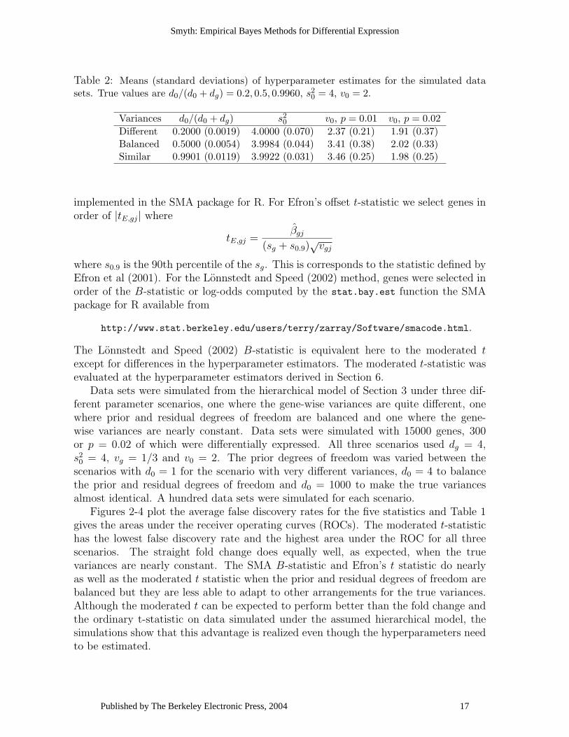
Table 2: Means (standard deviations) of hyperparameter estimates for the simulated datasets. True values are d0/(d0 + dg) = 0.2, 0.5, 0.9960, s2

0 = 4, v0 = 2.

Variances d0/(d0 + dg) s20 v0, p = 0.01 v0, p = 0.02

Different 0.2000 (0.0019) 4.0000 (0.070) 2.37 (0.21) 1.91 (0.37)Balanced 0.5000 (0.0054) 3.9984 (0.044) 3.41 (0.38) 2.02 (0.33)Similar 0.9901 (0.0119) 3.9922 (0.031) 3.46 (0.25) 1.98 (0.25)

implemented in the SMA package for R. For Efron’s offset t-statistic we select genes inorder of |tE,gj| where

tE,gj =βgj

(sg + s0.9)√vgj

where s0.9 is the 90th percentile of the sg. This is corresponds to the statistic defined byEfron et al (2001). For the Lonnstedt and Speed (2002) method, genes were selected inorder of the B-statistic or log-odds computed by the stat.bay.est function the SMApackage for R available from

http://www.stat.berkeley.edu/users/terry/zarray/Software/smacode.html.

The Lonnstedt and Speed (2002) B-statistic is equivalent here to the moderated texcept for differences in the hyperparameter estimators. The moderated t-statistic wasevaluated at the hyperparameter estimators derived in Section 6.

Data sets were simulated from the hierarchical model of Section 3 under three dif-ferent parameter scenarios, one where the gene-wise variances are quite different, onewhere prior and residual degrees of freedom are balanced and one where the gene-wise variances are nearly constant. Data sets were simulated with 15000 genes, 300or p = 0.02 of which were differentially expressed. All three scenarios used dg = 4,s20 = 4, vg = 1/3 and v0 = 2. The prior degrees of freedom was varied between the

scenarios with d0 = 1 for the scenario with very different variances, d0 = 4 to balancethe prior and residual degrees of freedom and d0 = 1000 to make the true variancesalmost identical. A hundred data sets were simulated for each scenario.

Figures 2-4 plot the average false discovery rates for the five statistics and Table 1gives the areas under the receiver operating curves (ROCs). The moderated t-statistichas the lowest false discovery rate and the highest area under the ROC for all threescenarios. The straight fold change does equally well, as expected, when the truevariances are nearly constant. The SMA B-statistic and Efron’s t statistic do nearlyas well as the moderated t statistic when the prior and residual degrees of freedom arebalanced but they are less able to adapt to other arrangements for the true variances.Although the moderated t can be expected to perform better than the fold change andthe ordinary t-statistic on data simulated under the assumed hierarchical model, thesimulations show that this advantage is realized even though the hyperparameters needto be estimated.

17



Table 2 give means and standard deviations of the hyperparameter estimates forthe simulated data sets. The estimates for d0/(d0 + dg) and s2

0 were very accurate.The estimator for v0 was nearly unbiased when p was set to the true proportion ofdifferentially expressed genes (p = 0.02) but was somewhat over-estimated when theproportion was set to a lower value (p = 0.01). As expected the estimator for v0 issomewhat more variable than that of d0/(d0 + dg) or s2

0. The results shown in Table 2are not affected by the prior limits on v0s

20 discussed in Section 6.

9 Data Examples

9.1 Swirl

Consider the Swirl data set which is distributed as part of the marrayInput packagefor R (Dudoit and Yang, 2003). The experiment was carried out using zebrafish as amodel organism to study the early development in vertebrates. Swirl is a point mutantin the BMP2 gene that affects the dorsal/ventral body axis. The main goal of the Swirlexperiment is to identify genes with altered expression in the Swirl mutant comparedto wild-type zebrafish. The experiment used four arrays in two dye-swap pairs. Themicroarrays used in this experiment were printed with 8448 probes (spots) including768 control spots. The hybridized microarrays were scanned with an Axon scannerand SPOT image analysis software (Buckley, 2000) was used to capture red and greenintensities for each spot. The data was normalized using print-tip loess normalizationand between arrays scale normalization using the LIMMA package (Smyth, 2003). Loessnormalization used window span 0.3 and three robustifying iterations.

For this data all genes have dg = 3 and vg = 1/4. The estimated prior degreesof freedom are d0 = 4.17 showing that posterior variances will be balanced betweenthe prior and sample variances with only slightly more weight to the former. Theestimated prior variance is s2

0 = 0.0509 which is less then the mean variance at 0.109but more than the median at 0.047. The estimated unscaled variance for the contrastis v0 = 22.7, meaning that the standard deviation of the log-ratio for a typical gene is(0.0509)1/2(22.7)1/2 = 1.07, i.e., genes which are differentially expressed typically changeby about two-fold. The prior limits on v0s

20 discussed in Section 6 do not come into

play for this data. The proportion of differentially expressed genes was set to p = 0.01following the default in the earlier SMA software. This value seems broadly realistic forsingle-gene knock-out vs wild-type experiments but is probably conservative for otherexperiments where more differential expression is expected.

Table 3 shows the top 30 genes as ranked by the B-statistic. The table includesthe fold change (or M-value), the ordinary t-statistic, the moderated t-statistic andthe B-statistic for the each gene. The moderated t and the B-statistics are evaluatedat the hyperparameter estimators derived in Section 6. There are no missing valuesfor this data so the two statistics necessarily give the same ranking of the genes. Theordinary t-statistics are on 3 degrees of freedom while the moderated t are on 7.17. Themoderated t-statistic method here ranks both copies of the knock-out gene BMP2 first

18



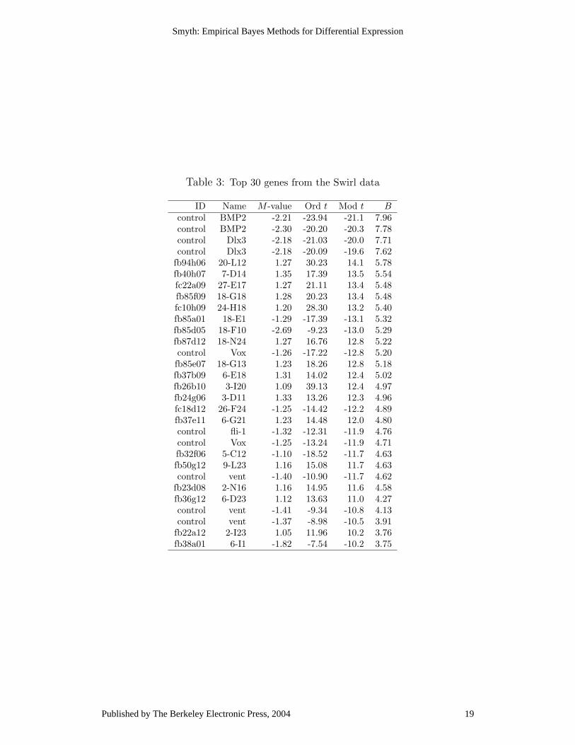
Table 3: Top 30 genes from the Swirl data

ID Name M -value Ord t Mod t Bcontrol BMP2 -2.21 -23.94 -21.1 7.96control BMP2 -2.30 -20.20 -20.3 7.78control Dlx3 -2.18 -21.03 -20.0 7.71control Dlx3 -2.18 -20.09 -19.6 7.62

fb94h06 20-L12 1.27 30.23 14.1 5.78fb40h07 7-D14 1.35 17.39 13.5 5.54fc22a09 27-E17 1.27 21.11 13.4 5.48fb85f09 18-G18 1.28 20.23 13.4 5.48fc10h09 24-H18 1.20 28.30 13.2 5.40fb85a01 18-E1 -1.29 -17.39 -13.1 5.32fb85d05 18-F10 -2.69 -9.23 -13.0 5.29fb87d12 18-N24 1.27 16.76 12.8 5.22control Vox -1.26 -17.22 -12.8 5.20fb85e07 18-G13 1.23 18.26 12.8 5.18fb37b09 6-E18 1.31 14.02 12.4 5.02fb26b10 3-I20 1.09 39.13 12.4 4.97fb24g06 3-D11 1.33 13.26 12.3 4.96fc18d12 26-F24 -1.25 -14.42 -12.2 4.89fb37e11 6-G21 1.23 14.48 12.0 4.80control fli-1 -1.32 -12.31 -11.9 4.76control Vox -1.25 -13.24 -11.9 4.71fb32f06 5-C12 -1.10 -18.52 -11.7 4.63fb50g12 9-L23 1.16 15.08 11.7 4.63control vent -1.40 -10.90 -11.7 4.62

fb23d08 2-N16 1.16 14.95 11.6 4.58fb36g12 6-D23 1.12 13.63 11.0 4.27control vent -1.41 -9.34 -10.8 4.13control vent -1.37 -8.98 -10.5 3.91fb22a12 2-I23 1.05 11.96 10.2 3.76fb38a01 6-I1 -1.82 -7.54 -10.2 3.75

19



and both copies of Dlx3, which is a known target of BMP2, second. Neither the foldchange nor the ordinary t-statistic do this. In general the moderated methods give amore predictable ranking of the control genes.

9.2 ApoAI

These data are from a study of lipid metabolism by Callow et al (2000) and are availablefrom

http://www.stat.berkeley.edu/users/terry/zarray/Html/matt.html.

The apolipoprotein AI (ApoAI) gene is known to play a pivotal role in high densitylipoprotein (HDL) metabolism. Mouse which have the ApoAI gene knocked out havevery low HDL cholesterol levels. The purpose of this experiment is to determine howApoAI deficiency affects the action of other genes in the liver, with the idea that thiswill help determine the molecular pathways through which ApoAI operates.

The experiment compared 8 ApoAI knockout mice with 8 normal C57BL/6 mice,the control mice. For each of these 16 mice, target mRNA was obtained from livertissue and labelled using a Cy5 dye. The RNA from each mouse was hybridized to aseparate microarray. Common reference RNA was labelled with Cy3 dye and used forall the arrays. The reference RNA was obtained by pooling RNA extracted from the8 control mice. Although still a simple design, this experiment takes us outside thereplicated array structure considered by Lonnstedt and Speed (2002).

Intensity data was captured from the array images using SPOT software and thedata was normalized using print-tip loess normalization. The normalized intensitieswere analyzed for differential expression by fitting a two-parameter linear model, theparameter of interest measuring the difference between the ApoAI knockout line andthe control mice.

The residual degrees of freedom are dg = 14 for most genes but some have dg as lowas 10. The estimated prior degrees of freedom are d0 = 3.7. The residual degrees offreedom are relatively large here so the sample variances will be shrunk only slightly andthe moderated and ordinary t-statistics will differ substantially only when the samplevariance is unusually small. The prior variance is s2

0 = 0.048 which is somewhat lessthan the median sample variance at 0.064. The unscaled variance for the contrasts ofinterest is estimated to be v0 = 3.4 meaning that the typical fold change for differentiallyexpressed genes is estimated to be about 1.3. Prior limits on v0s

20 do not come into play

for these data.Table 4 shows the top 15 genes as ranked by the B-statistic for the parameter of

interest. The moderated t rank the genes in the same order even though there are afew missing values for this data. The top gene is ApoAI itself which is heavily down-regulated as expected. Several of the other genes are closely related to ApoAI. Thetop eight genes here have been confirmed to be differentially expressed in the knockoutversus the control line (Callow et al, 2000). For these data the top eight genes standout clearly from the other genes and all methods clearly separate these genes from the

20



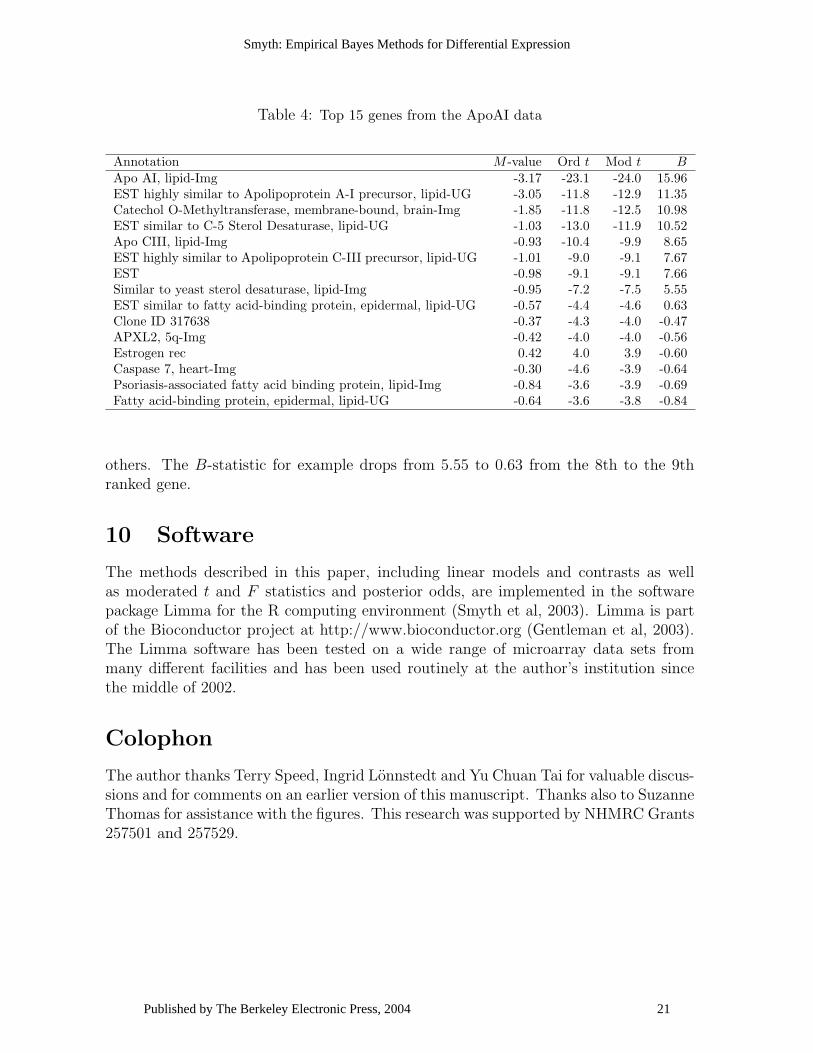
Table 4: Top 15 genes from the ApoAI data

Annotation M -value Ord t Mod t BApo AI, lipid-Img -3.17 -23.1 -24.0 15.96EST highly similar to Apolipoprotein A-I precursor, lipid-UG -3.05 -11.8 -12.9 11.35Catechol O-Methyltransferase, membrane-bound, brain-Img -1.85 -11.8 -12.5 10.98EST similar to C-5 Sterol Desaturase, lipid-UG -1.03 -13.0 -11.9 10.52Apo CIII, lipid-Img -0.93 -10.4 -9.9 8.65EST highly similar to Apolipoprotein C-III precursor, lipid-UG -1.01 -9.0 -9.1 7.67EST -0.98 -9.1 -9.1 7.66Similar to yeast sterol desaturase, lipid-Img -0.95 -7.2 -7.5 5.55EST similar to fatty acid-binding protein, epidermal, lipid-UG -0.57 -4.4 -4.6 0.63Clone ID 317638 -0.37 -4.3 -4.0 -0.47APXL2, 5q-Img -0.42 -4.0 -4.0 -0.56Estrogen rec 0.42 4.0 3.9 -0.60Caspase 7, heart-Img -0.30 -4.6 -3.9 -0.64Psoriasis-associated fatty acid binding protein, lipid-Img -0.84 -3.6 -3.9 -0.69Fatty acid-binding protein, epidermal, lipid-UG -0.64 -3.6 -3.8 -0.84

others. The B-statistic for example drops from 5.55 to 0.63 from the 8th to the 9thranked gene.

10 Software

The methods described in this paper, including linear models and contrasts as wellas moderated t and F statistics and posterior odds, are implemented in the softwarepackage Limma for the R computing environment (Smyth et al, 2003). Limma is partof the Bioconductor project at http://www.bioconductor.org (Gentleman et al, 2003).The Limma software has been tested on a wide range of microarray data sets frommany different facilities and has been used routinely at the author’s institution sincethe middle of 2002.

Colophon

The author thanks Terry Speed, Ingrid Lonnstedt and Yu Chuan Tai for valuable discus-sions and for comments on an earlier version of this manuscript. Thanks also to SuzanneThomas for assistance with the figures. This research was supported by NHMRC Grants257501 and 257529.

21



Appendix: Inversion of Trigamma Function

In this appendix we solve ψ′(y) = x for y where x > 0 by deriving a Newton iterationwith guaranteed and rapid convergence.

Define f(y) = 1/ψ′(y). The function f is nearly linear and convex for y > 0,satisfying f(0) = 0 and asymptoting to f(y) = y − 0.5 as y →∞. The first derivative

f ′(y) = − ψ′′(y)

ψ′(y)2

is strictly increasing from f ′(0) = 0 to f ′(∞) = 1. This means that the Newton iterationto solve f(y) = z for y is monotonically convergent provided that the starting value y0

satisfies f(y0) ≥ z. Such a starting value is provided by y0 = 0.5 + z.The complete Newton iteration to solve ψ′(y) = x is as follows. Set y0 = 0.5 + 1/x.

Then iterate yi+1 = yi + δi with δi = ψ′(yi){1−ψ′(yi)/x}/ψ′′(yi) until −δi/y < ε whereε is a small positive number. The step δi is strictly negative unless ψ′(yi) = x. Using64-bit double precision arithmetic, ε = 10−8 is adequate to achieve close to machineprecision accuracy. To avoid overflow or underflow in floating point arithmetic, we canset y = 1/

√x when x > 107 and y = 1/x when x < 10−6 instead of performing the

iteration. Again these choices are adequate for nearly full precision in 64-bit arithmetic.

References

Baldi, P., and Long, A. D. (2001). A Bayesian framework for the analysis of microar-ray expression data: regularized t-test and statistical inferences of gene changes.Bioinformatics 17, 509–519.

Broberg, P. (2003). Statistical methods for ranking differentially expressed genes.Genome Biology 4: R41.

Buckley, M. J. (2000). Spot User’s Guide. CSIRO Mathematical and InformationSciences, Sydney, Australia. http://www.cmis.csiro.au/iap/Spot/spotmanual.htm.

Callow, M. J., Dudoit, S., Gong, E. L., Speed, T. P., and Rubin, E. M. (2000). Mi-croarray expression profiling identifies genes with altered expression in HDL deficientmice. Genome Research 10, 2022–2029.

Chu, T.-M., Weir, B., and Wolfinger, R. (2002). A systematic statistical linear modelingapproach to oligonucleotide array experiments. Mathematical Biosciences 176, 35–51.

Cui, X., and Churchill, G. A. (2003). Statistical tests for differential expression incDNA microarray experiments. Genome Biology 4, 210.1–210.9.

Dudoit, S., and Yang, Y. H. (2003). Bioconductor R packages for exploratory analysisand normalization of cDNA microarray data. In G. Parmigiani, E. S. Garrett, R. A.

22



Irizarry and S. L. Zeger, editors, The Analysis of Gene Expression Data: Methodsand Software, Springer, New York. pp. 73-101.

Efron, B. (2003). Robbins, empirical Bayes and microarrays. Annals of Statistics 31,366–378.

Efron B., Tibshirani, R., Storey J. D., and Tusher V. (2001). Empirical Bayes analysisof a microarray experiment. Journal of the American Statistical Association 96,1151–1160.

Ferkingstad, E., Langaas, M., and Lindqvist, B. (2003). Estimating the proportion oftrue null hypotheses, with application to DNA microarray data. Preprint StatisticsNo. 4/2003, Norwegian University of Science and Technology, Trondheim, Norway.http://www.math.ntnu.no/preprint/

Ge, Y., Dudoit, S., and Speed, T. P. (2003). Resampling-based multiple testing formicroarray data analysis, with discussion. TEST 12, 1–78.

Gentleman, R., Bates, D., Bolstad, B., Carey, V., Dettling, M., Dudoit, S., Ellis, B.,Gautier, L., Gentry, J., Hornik, K., Hothorn, T., Huber, W., Iacus, S., Irizarry, R.,Leisch, F., C., Maechler, M., Rossini, A. J., Sawitzki, G., Smyth, G. K., Tierney,L., Yang, J. Y. H., and Zhang, J. (2003). Bioconductor: a software developmentproject. Technical Report November 2003, Department of Biostatistics, HarvardSchool of Public Health, Boston.

Huber, W., von Heydebreck, A., Sltmann, H., Poustka, A., and Vingron, M. (2002).Variance stabilization applied to microarray data calibration and to the quantifica-tion of differential expression. Bioinformatics 18, S96–S104.

Ibrahim, J. G., Chen, M.-H., and Gray, R. J. (2002). Bayesian models for gene expres-sion with DNA microarray data. Journal of the American Statistical Society 97,88-99.

Irizarry, R. A., Bolstad, B. M., Francois Collin, F., Cope, L. M., Hobbs, B., and Speed,T. P. (2003), Summaries of Affymetrix GeneChip probe level data. Nucleic AcidsResearch 31(4):e15.

Jin, W., Riley, R. M., Wolfinger, R. D., White, K. P., Passador-Gurgel, G., and Gibson,G. (2001). The contributions of sex, genotype and age to transcriptional variancein Drosophila melanogaster. Nature Genetics 29, 389–395.

Johnson, N. L., and Kotz, S. (1970). Distributions in Statistics: Continuous UnivariateDistributions – 2. Wiley, New York.

Kendziorski, C. M., Newton, M. A., Lan, H., and Gould, M. N. (2003). On paramet-ric empirical Bayes methods for comparing multiple groups using replicated geneexpression profiles. Statistics in Medicine. To appear.

23



Kerr, M. K., and Churchill, G. A. (2001). Experimental design for gene expressionmicroarrays. Biostatistics 2, 183–201.

Kerr, M. K., Martin, M., and Churchill, G. A. (2000). Analysis of variance for geneexpression microarray data. Journal of Computational Biology 7, 819–837.

Li, C., and Wong, W. H. (2001). Model-based analysis of oligonucleotide arrays: expres-sion index computation and outlier detection. Proceedings of the National Academyof Sciences 98, 31–36.

Lonnstedt, I. (2001). Replicated Microarray Data. Licentiate Thesis, Department ofMathematics, Uppsala University.

Lonnstedt, I., Grant, S., Begley, G., and Speed, T. P. (2003). Microarray analysis oftwo interacting treatments: a linear model and trends in expression over time. Toappear.

Lonnstedt, I., and Speed, T. P. (2002). Replicated microarray data. Statistica Sinica12, 31–46.

Nature Genetics Editors (eds.) (2003). Chipping Forecast II. Nature Genetics Supple-ment 32, 461–552.

Newton, M.A. and Kendziorski, C. M. (2003). Parametric empirical Bayes methodsfor microarrays. In: The analysis of gene expression data: methods and software.Eds. G. Parmigiani, E. S. Garrett, R. Irizarry and S. L. Zeger, Springer Verlag, NewYork. To appear.

Newton, M. A., Kenziorski, C. M., Richmond, C. S., Blattner, F. R., and Tsui, K. W.(2001). On differential variability of expression ratios: improving statistical inferenceabout gene expression changes from microarray data. Journal of ComputationalBiology 8, 37–52.

Parmigiani, G., Garrett, E. S., Irizarry, R. A., and Zeger, S. L. (eds.) (2003). TheAnalysis of Gene Expression Data: Methods and Software. Springer, New York.

Smyth, G. K., Thorne, N. P., and Wettenhall, J. (2003). Limma: Linear Models for Mi-croarray Data User’s Guide. Software manual available from http://www.biocond-uctor.org.

Smyth, G. K., and Speed, T. P. (2003). Normalization of cDNA microarray data. In:METHODS: Selecting Candidate Genes from DNA Array Screens: Application toNeuroscience, D. Carter (ed.). Methods Volume 31, Issue 4, December 2003, pages265–273.

Smyth, G. K., Yang, Y.-H., Speed, T. P. (2003). Statistical issues in microarray dataanalysis. In: Functional Genomics: Methods and Protocols, M. J. Brownstein andA. B. Khodursky (eds.), Methods in Molecular Biology Volume 224, Humana Press,Totowa, NJ, pages 111–136.

24



Speed, T. P. (ed.) (2003). Statistical Analysis of Gene Expression Microarray Data.Chapman & Hall/CRC, Boca Raton.

Tusher, V. G., Tibshirani, R., and Chu, G. (2001). Significance analysis of microarraysapplied to the ionizing radiation response. PNAS 98, 5116–5121.

Wolfinger, R. D., Gibson, G., Wolfinger, E. D., Bennett, L., Hamadeh, H., Bushel,P., Afshari, C., and Paules, R. S. (2001). Assessing gene significance from cDNAmicroarray expression data via mixed models. Journal of Computational Biology 8,625–637.

Yang, Y. H., and Speed, T. P. (2003). Design and analysis of comparative microarrayexperiments. In T. P. Speed (ed.), Statistical Analysis of Gene Expression Microar-ray Data, Chapman & Hall/CRC Press, pages 35–91.

25



Documents

Statistical Applications in Genetics and Molecular Biologyyekutiel/eBayes/smyth_2004.pdf · Volume 3, Issue 1 2004 Article 3 Statistical Applications in Genetics and Molecular Biology