Statistical Applications in Genetics and Molecular Biologyyekutiel/papers/SAGMB -- Dan Lin.pdf · Directional inference to testing ... Statistical Applications in Genetics and Molecular

Statistical Applications in Geneticsand Molecular Biology

Volume6, Issue1 2007 Article 26

Testing for Trends in Dose-ResponseMicroarray Experiments: A Comparison ofSeveral Testing Procedures, Multiplicity and

Resampling-Based Inference

Dan Lin∗ Ziv Shkedy† Dani Yekutieli‡

Tomasz Burzykowski∗∗ Hinrich W.H. Gohlmann†† An De Bondt‡‡

Tim Perera§ Tamara Geerts¶ Luc Bijnens‖

∗Hasselt University, [email protected]†Hasselt University, [email protected]‡Tel Aviv University, [email protected]

∗∗Hasselt University, [email protected]††Johnson & Johnson PRD, [email protected]‡‡Johnson & Johnson PRD, [email protected]§Johnson & Johnson PRD, [email protected]¶Johnson & Johnson PRD, [email protected]‖Johnson & Johnson PRD, [email protected]

Copyright c©2007 The Berkeley Electronic Press. All rights reserved.

Testing for Trends in Dose-ResponseMicroarray Experiments: A Comparison ofSeveral Testing Procedures, Multiplicity and

Resampling-Based Inference∗

Dan Lin, Ziv Shkedy, Dani Yekutieli, Tomasz Burzykowski, Hinrich W.H.Gohlmann, An De Bondt, Tim Perera, Tamara Geerts, and Luc Bijnens

Abstract

Dose-response studies are commonly used in experiments in pharmaceutical research in orderto investigate the dependence of the response on dose, i.e., a trend of the response level toxicitywith respect to dose. In this paper we focus on dose-response experiments within a microarraysetting in which several microarrays are available for a sequence of increasing dose levels. A geneis called differentially expressed if there is a monotonic trend (with respect to dose) in the gene ex-pression. We review several testing procedures which can be used in order to test equality amongthe gene expression means against ordered alternatives with respect to dose, namely Williams’(Williams 1971 and 1972), Marcus’ (Marcus 1976), global likelihood ratio test (Bartholomew1961, Barlow et al. 1972, and Robertson et al. 1988), and M (Hu et al. 2005) statistics. Ad-ditionally we introduce a modification to the standard error of the M statistic. We compare theperformance of these five test statistics. Moreover, we discuss the issue of one-sided versus two-sided testing procedures. False Discovery Rate (Benjamni and Hochberg 1995, Ge et al. 2003),and resampling-based Familywise Error Rate (Westfall and Young 1993) are used to handle themultiple testing issue. The methods above are applied to a data set with 4 doses (3 arrays per dose)and 16,998 genes. Results on the number of significant genes from each statistic are discussed.A simulation study is conducted to investigate the power of each statistic. A R library IsoGeneimplementing the methods is available from the first author.

KEYWORDS: dose response study, multiple testing, monotonicity, resampling-based procedures

∗Financial support from the IAP research network nr P5/24 of the Belgian Government (BelgianScience Policy) is gratefully acknowledged.

1 Introduction

Investigation of a dose-response relationship is of primary interest in manydrug-development studies. Typically, in dose-response experiments the out-come of interest is measured at several (increasing) dose levels, and the aimof the analysis is to establish the form of the dependence of the response ondose (Agresti 1997). The response can be either the efficacy of a treatmentor the risk associated with the exposure to the treatment (in toxicology stud-ies). In a typical dose-response study subjects are randomized to several dosegroups, among which there is usually a control group. Ruberg (1995a, 1995b)and Chuang-Stein and Agresti (1997) formulated four main questions usuallyasked in dose-response studies: (1) Is there any evidence of the drug effect?(2) For which doses is the response different from the response in the controlgroup? (3) What is the nature of the dose-response relationship? and (4)What is the optimal dose?

Within the microarray setting, a dose-response experiment has the samestructure as described above. The response is the gene expression at a certaindose level. The dose-response curve, similarly to the dose-response studies, isassumed to be monotone, i.e., the gene activity increases or decreases as thedose level increases. The direction of the relationship is usually unknown inadvance.

In this paper we focus on the first question: is there any evidence of thedrug effect? To answer this question, we test for the null hypothesis of homo-geneity of means (no dose effect) against an ordered alternative. We compareseveral testing procedures, that take into account the order restriction of themeans with respect to the increasing doses and that adjust for multiplicity. Inparticular, we discuss the testing procedures of Williams (Williams 1971 and1972), Marcus (Marcus 1976), the global likelihood ratio test (Barlow et al.1972, and Robertson et al. 1988), and the M (Hu et al. 2005) statistic. More-over, we propose a novel procedure based on a modification of the estimatorof standard error of the M statistic.

Williams (1971, 1972) proposed a step-down procedure to test for the doseeffect. The tests are performed sequentially from the comparison between theisotonic mean of the highest dose and the sample mean of the control to thecomparison between the isotonic mean of the lowest dose and the sample meanof the control. The procedure stops at the dose level where the null hypothesis(of no dose effect) is not rejected. Marcus (1976) proposed a modification ofthe Williams procedure, in which the sample mean of the control was replacedby the isotonic mean of the control. A global likelihood ratio test discussedby Bartholomew et al. (1961), Barlow et al. (1972), and Robertson et al.,

1

Lin et al.: Testing for Monotonic Trends for Gene Expression Data

Published by The Berkeley Electronic Press, 2007

(1988) uses the ratio between the variance calculated under the null hypothesisand the variance calculated under an ordered alternative. Recently, Hu et al.(2005) proposed a test statistic that was similar to Marcus’ statistic, but withthe variance estimator calculated under the ordered alternative. The degrees offreedom of the M statistic (the difference between the number of observationsand the number of dose levels) are fixed for all the genes and all the arrays.In this paper, we propose a modification for the variance estimator of the Mstatistic. Namely, the difference between the number of observations and theunique number of isotonic means is used as the degrees of freedom for thevariance estimator.

Our goal is to compare the performance of the five test statistics. To thisaim we apply them to a case study. The case study data come from a microar-ray experiment with three microarrays, each containing 16,998 genes, availablefor each of four dose levels of a drug. When applied to the case study, thefive test statistics are adjusted for multiple testing by using resampling-basedprocedures that control either the Family-Wise Error Rate (FWER) or theFalse Discovery Rate (FDR). Following the results of the analysis of the casestudy, we conduct a simulation study to further investigate the performanceof the five test statistics.

The paper is organized as follows. Section 2 describes the procedure fol-lowed to obtain the case study data. In Section 3 we review the five teststatistics. Directional inference to testing isotonic regression and multiplic-ity issue are discussed in Section 4. In Section 5 we compare the results ofthe analysis of the case study using the five tests discussed in Section 3. Asimulation study conducted to investigate the performance of variance estima-tors and power of the five test statistics is presented in Section 6. Section 7completes the paper with a short discussion.

2 Data Acquisition

The human epidermal squamous carcinoma cell line A431 was grown in Dul-becco’s modified Eagle’s medium, supplemented with Lglutamine (2 mM),Gentamycin (50 mg/ml) and 10% fetal bovine serum. The cells were stimu-lated with EGF (R&D Systems, 236-EG) at different concentrations (0 ng/ml,1 ng/ml, 10 ng/ml and 100 ng/ml) for 24h. RNA was harvested using RLTbuffer (Qiagen). All microarray related steps, including the amplification of to-tal RNAs, labeling, hybridization and scanning were carried out as describedin the GeneChip Expression Analysis Technical Manual, Rev.4 (Affymetrix2004). Biotin-labeled target samples were hybridized to human genome ar-

2

Statistical Applications in Genetics and Molecular Biology, Vol. 6 [2007], Iss. 1, Art. 26

http://www.bepress.com/sagmb/vol6/iss1/art26

rays U133 A 2.0 containing probe sets interrogation approximately 22,000transcripts from the UniGene database (Build 133). Hybridization was per-formed using 15 µg of cRNA for 16 h at 450C under continuous rotationat 60 rpm. Arrays were stained in Affymetrix Fluidics stations using strep-tavidin/phycoerythrin staining. Thereafter, arrays were scanned with theAffymetrix scanner 3000, and images were analyzed using the GeneChip Op-erating System v1.1 (GCOS, Affymetrix). The collected data were quantilenormalized in two steps: first within each sample group, and then across allsample groups obtained (Bolstad et al. 2002). The resulting data set consistsof 12 samples, for four dose levels and three microarrays at each dose level,with 16,998 probe sets. For simplicity, we refer to probe sets as genes throughour paper (Hubbell et al. 2002).

3 Testing For Homogeneity of the Means Un-

der Restricted Alternatives

In this section, we discuss several procedures for testing the homogeneity ofthe means under the restricted alternative. In particular we focus on fourexisting procedures: Williams’ (Williams 1971 and 1972), Marcus’ (Marcus1976), the global likelihood ratio test (Bartholomew 1961, Barlow et al. 1972,and Robertson et al. 1988), and the M (Hu et al. 2005) statistic. Additionally,we introduce a modification to the degree of freedom of the M statistic.

In the microarray experiment, for each gene, the following ANOVA modelis considered

Yij = µ(di) + εij, i = 0, 1, . . . , K, j = 1, 2, . . . , ni, (1)

where Yij is the jth gene expression at the ith dose level, di (i = 0, 1, . . . , K)are the K+1 dose levels, µ(di) is the mean gene expression at each dose level,and εij ∼ N(0, σ2).

The null hypothesis of no dose effect is given by

H0 : µ(d0) = µ(d1) = · · · = µ(dK). (2)

A one-sided alternative hypothesis of a positive dose effect for at least one doselevel (i.e., an increasing trend) is specified by

HUp1 : µ(d0) ≤ µ(d1) ≤ · · · ≤ µ(dK), (3)

with at least one strict inequality. When testing the affect of a drug for apositive outcome the researcher can specify a positive effect as the desirable

3



alternative. However, in the current microarray setting, it seems reasonableto assume that the gene expression levels may increase or decrease in responseto increasing doses, but with the direction of the trend not known in advance.Thus we must also consider an additional alternative:

HDown1 : µ(d0) ≥ µ(d1) ≥ · · · ≥ µ(dK), (4)

with at least one strict inequality. Testing H0 against HDown1 or HUp

1 requiresestimation of the means under both the null and the alternative hypotheses.Under the null hypothesis, the estimator for the mean response µ is the samplemean. Let µ?

0, µ?1, . . . , µ

?K be the maximum likelihood estimates for the means

(at each dose level) under the ordered alternative. Barlow et al. (1972) andRobertson et al. (1998) showed that µ?

0, µ?1, . . . , µ

?K are the isotonic regression

of the observed means.

3.1 Williams’ (1971, 1972) and Marcus’ (1976) Test Sta-tistics

Williams’ procedure defines H0 as the null hypothesis, and HUp1 or HDown

1 asthe one-sided alternative. Williams’ (1971, 1972) test statistics was suggestedfor a setting, in which ni observations are available at each dose level. As alldose levels are compared with the control level, the test statistic is given by

ti =µ?

i − y0√2S2/r

. (5)

Here, y0 is the sample mean at the first dose level (control), µ?i is the estimate

for the mean at the ith dose level under the ordered alternative, r is the numberof replications at each dose level, and S2 is an estimate of the variance. Forµ?

i , Williams (1971, 1972) used the isotonic regression of the observed responsewith respect to dose (Barlow et al. 1972). Williams’ test procedure is asequential procedure. In the first step, µ?

K is compared to y0. If the nullhypothesis is rejected, µ?

K−1 is compared to y0, etc.Marcus (1976) proposed a modification to Williams’ test statistic that re-

placed y0 with µ?0, the estimate of the first dose (control) mean under ordered

restriction. Marcus’ test statistic performs closely to Williams’ in terms ofpower (Marcus 1976). Note that, for K = 1, Williams’ and Marcus’ teststatistics reduce to the two-sample t-test.

4



3.2 Likelihood Ratio Test Statistic for Monotonicity(Barlow et al. 1972, and Robertson et al. 1988)

Williams’ and Marcus’ procedures are step-down procedures, i.e., the compar-ison between a lower dose and control is tested only if the test of a higherdose vs. control is significant. The underlying assumption is that there is amonotone dose-response relationship with a known direction.

Testing the equality of ordered means using likelihood ratio tests (whenresponse is assumed to be normally distributed) were discussed by Barlowet al. (1972) and Robertson et al. (1988). Both authors considered thelikelihood ratio test, in which the variance under the null and the alternativewere compared. The likelihood ratio test statistic is given by

Λ2N01 =

σ2H1

σ2H0

=

∑ij(yij − µ?

j)2

∑ij(yij − µ)2

, (6)

where σ2H0

and σ2H1

are the parameter estimates for the variance under the nulland the alternative hypothesis, respectively. The null hypothesis is rejected

for a “small” value of Λ2N01. Equivalently, H0 is rejected for large value of E2

01,where

E201 = 1− Λ

2N01 =

∑ij(yij − µ)2 −∑

ij(yij − µ?j)

2

∑ij(yij − µ)2

. (7)

Estimating the parameters using isotonic regression requires the knowledge ofthe direction of the trend. In practice, the direction of the trend is often notknown in advance. In such a case one can maximize the likelihood twice: fora monotone decreasing trend and for a monotone increasing trend, and choosethe trend with a higher likelihood. In practice, we can calculate E2

01 for eachdirection and choose the higher value of E2

01 (Barlow et al. 1972). In this paperwe use a resampling-based approach to approximate the null distribution forthe test statistic, so that the two sided p-values are obtained for inference.

3.3 The M Test Statistic of Hu et al. (2005)

Recently, Hu et al. (2005) proposed the following test statistic M to test fora monotonic trend:

M =µ?

K − µ?0√∑K

i=0

∑ni

j=1(yij − µ?i )

2/(N −K). (8)

Hu et al. (2005) discussed a setting, in which the comparison of primaryinterest is the difference between the highest dose level (K) and the control

5



dose. The numerator of the M test statistic is the same as of Marcus’ statistic,while the denominator is an estimate of the standard error under an orderedalternative. This is in contrast to Williams’ and Marcus’ approaches that usethe unrestricted means to derive the estimate for the standard error.

Hu et al. (2005) evaluated the performance of the E201 and M test statistics

by comparing the ranks of genes obtained by using both statistics, and reportedsimilar findings for simulated and real life data sets.

3.4 A Modification to the M test Statistic

For the variance estimate, Hu et al. (2005) used N − K degrees of freedom(see equation (8)). However, the unique number of isotonic means is not fixed,but changes across the genes. For that reason, we propose a modificationto the standard error estimator used in the M statistic by replacing it with√∑K

i=0

∑ni

j=1(yij − µ?i )

2/(N − I), where I is the unique number of isotonic

means for a given gene. Such a modification is expected to improve the stan-dard error estimates across all the genes.

4 Directional Inference in Isotonic Regression

and Multiplicity

4.1 Multiplicity and Resampling-based Multiple Test-ing

In microarray experiments a large of number of null hypotheses usually needsto be tested. The FamilyWise Error Rate (FWER, Westfall and Young 1993)and the False Discovery Rate (FDR, Benjamini and Hochberg 1995) are twoquantities that are commonly used in controlling the error rate.

FWER is defined as the probability to reject at least one true null hypoth-esis. FDR, introduced by Benjamini and Hochberg (1995), is defined as theexpected proportion of false rejections among the rejected hypotheses. Test-ing procedures that control FDR tend to gain more power as compared toprocedures controlling for FWER.

FWER can be controlled by using, e.g., the Bonferroni, Holm (Holm 1979),Hochberg (1995), or maxT (Westfall and Young 1993) procedures. Hochbergand Benjamini (FDR-BH, 1995) and Benjamini and Yekutieli (FDR-BY, 1999)proposed approaches for controlling FDR.

6



In a microarray setting, resampling methods to adjust for multiplicity areoften used (Kerr and Churchill 2001, Reiner et al. 2003, Tusher et al. 2001, andGe et al. 2003). The main motivation is to avoid inference based on asymptoticdistribution of the test statistics, which, within the microarray setting, can beproblematic because of either typically small sample sizes or departure fromthe assumption about the distribution of the response. Also, in some casesthe asymptotic distribution of the test statistics is unknown (Tusher et al.2001). The resampling approach requires permutation of the sample labels,and calculation of the test statistic for each permutation. Matrix of the valuesof the test statistic for each gene and for each permutation is referred to as thepermutation matrix under the null distribution. Further inference is based onthe unadjusted p-values obtained from the permutation matrix. For example,maxT procedure proposed by Westfall and Young (1993) to control FWERcomputes the adjusted p-values from the distribution of maxima of the teststatistics over the nested subsets of ordered test statistics calculated underthe null hypothesis (by applying the permutation matrix). Alternatively, oncethe unadjusted p-values of a test statistic are computed (Reiner et al. 2003and Ge et al. 2003), they can be adjusted for multiple testing using variousprocedures such as Bonferroni, Holm, FDR-BH or FDR-BY.

4.2 Directional Inference in Isotonic Regression

The five test statistics discussed in Section 3 should be calculated assuminga particular direction of the ordered alternative. However, the direction ofthe test is unknown in advance. In this section, we address the issue of howto obtain the two-sided p-value from the five testing procedures, and how todetermine the direction of the trend from two-sided p-value afterwards.

We focus on the two possible directions of the alternatives: HUp1 defined in

equation (3) and HDown1 defined in equation (4). Let pUp and TUp denote the

p-value and the corresponding test statistic computed to test H0 vs. HUp1 , and

let pDown and TDown denote the p-value and the corresponding test statisticcomputed to test H0 vs. HDown

1 . Barlow et al. (1972) showed that, for K > 2,a χ2 statistic for testing H0 may actually yield pUp < α and pDown < α.However, p = 2 min(pUp, pDown) is always a conservative p-value for the two-sided test of H0 vs. either HUp

1 or HDown1 .

Hu et al. (2005) adapted the approach by taking the larger of the likeli-hoods of HUp

1 or HDown1 , i.e., the larger of TUp and TDown is used as the test

statistic for two-sided inference. In contrast to Hu et al. (2005), we obtain two-sided p-values by taking p = min(2 min(pUp, pDown), 1), where pUp and pDown

are calculated for TUp and TDown using permutations to approximate the null

7



distribution of these test statistics. We use pUp and pDown to determine thedirection of the test.

After rejecting the null hypothesis against the two-sided test there is stilla need to determine the direction of the trend. The direction can be in-ferred by the following procedure. If pUp ≤ α/2, then reject H0 and declareHUp

1 ; if pDown ≤ α/2, then reject H0 and declare HDown1 . The validity of this

directional inference is based on the following property: under HUp1 , pDown

is stochastically larger than U [0, 1]; and under HDown1 , pUp is stochastically

larger than U [0, 1]. Thus, the probability of falsely rejecting H0 is ≤ α, andthe probability of declaring a wrong direction for the trend is ≤ α/2. It isalso important to note that the event pUp < α/2 and pDown < α/2 may beobserved. Under H0, HUp

1 or HDown1 , this event is unlikely. However, it is

likely if the treatment has a large and non-monotone effect. An example ofthis unique situation, in which the null hypothesis can be rejected for bothdirections, is given in Section 5.1.

In order to verify whether the property needed for directional inferenceapplies to the five test statistics, we conduct a simulation study to investigatethe distribution of the pUp and pDown values. For each simulation, data aregenerated under HUp

1 : the means are assumed to be equal to (1, 2, 3, 4)/√

5for the four doses, respectively, and the variance is equal to σ2 = 1. Thetest statistics TUp and TDown are calculated for the two possible alternativesHUp

1 and HDown1 . Their corresponding pUp and pDown-values are obtained using

10,000 permutations.Figure 1 shows the cumulative distribution of pUp and pDown. Clearly,

the simulations show that the cumulative distribution of pDown (the p-valueof the test statistics calculated assuming the wrong direction, dotted line inFigure 1) is stochastically higher than U [0, 1] (solid line in Figure 1), whichis the distribution of the p-values under the null hypothesis. Moreover, thedistribution of pUp (the p-value for the test statistics calculated assuming theright direction, dashed line in Figure 1) is, as expected, stochastically smallerthan U([0, 1]. Similar results (not shown) are obtained when the data aregenerated under HDown

1 . The results imply that all the five test statisticsprocess the property required for the directional inference: under HUp

1 thedistribution of pDown is stochastically greater than U [0, 1]. Further discussionof the simulation results is given in the supplementary material to this paper.

4.3 Control of the Directional FDR

When FDR controlling procedures are used to adjust for multiplicity in themicroarray setting, the set of two-sided p-values computed for each gene is

8



0.0 0.2 0.4 0.6 0.8 1.0

0.0

0.2

0.4

0.6

0.8

1.0

p−values

cum

ulat

ive

p−va

lues

a: E2

0.0 0.2 0.4 0.6 0.8 1.0

0.0

0.2

0.4

0.6

0.8

1.0

p−values

cum

ulat

ive

p−va

lues

b: Williams

0.0 0.2 0.4 0.6 0.8 1.0

0.0

0.2

0.4

0.6

0.8

1.0

p−values

cum

ulat

ive

p−va

lues

c: Marcus

0.0 0.2 0.4 0.6 0.8 1.0

0.0

0.2

0.4

0.6

0.8

1.0

p−values

cum

ulat

ive

p−va

lues

d: M

0.0 0.2 0.4 0.6 0.8 1.0

0.0

0.2

0.4

0.6

0.8

1.0

p−values

cum

ulat

ive

p−va

lues

e: Modified M

Figure 1: The cumulative distribution of pUp-values (dashed line) and pDown-values (dotted line) for the five test statistics. Data are generated under HUp

1

with isotonic means (1, 2, 3, 4)/√

5 for the four doses. Solid line: cumulativedistribution of H0 ∼ U [0, 1].

adjusted using FDR-BH and FDR-BY procedure. A discovery in this case isa rejection of H0 for some gene; a false discovery is to reject H0 when H0 istrue. As mentioned before, in a microarray dose-response experiment we arealso interested in the direction of the dose-response trend.

Benjamini and Yekutieli (2005) provide a framework for addressing themultiplicity problem when attempting to determine the direction of multipleparameters: a discovery is to declare the sign of a parameter as either beingpositive or negative. Three types of false discoveries are possible: declaring azero parameter either as negative or as positive, declaring a negative param-eter as positive, and declaring a positive parameter as negative. The FDRcorresponding to these discoveries is termed the Mixed Directional FDR. Inthe current setting the Mixed Directional FDR is the expected value of thenumber of genes, for which H0 is true, that are erroneously declared to haveeither a positive or negative trend plus the genes with a monotone trend but

9



the direction of the declared trend is wrong, divided by the total number ofgenes declared to have a trend. Benjamini and Yekutieli (2005) prove that ifp-values pose the directional property described in Section 4.2, then applyingthe BH procedure at level q to the the set of two-sided p-values computed foreach gene, and declaring the direction of the trend corresponding to the smallerone-sided p-value, controls the Mixed Directional FDR at level q/2·(1+m0/m),where m is the total number of genes and m0 is the number of genes, for whichH0 holds.

In general, directional inference is a more general setting than hypothesestesting (Benjamini and Yekutieli, 2005). Nevertheless, as a false discovery ismade based on the p-value that is stochastically larger than U [0, 1], then theresampling-based methods that control FDR (Yekutieli and Benjamini, 1999)also control the Mixed Directional FDR. This is achieved by simply applyingthe resampling-based procedure to test H0, and if H0 is rejected, declaring thedirection of the trend according to the minimum one-sided p-value. For eachrejected null hypothesis it is also advisable to examine if the larger p-value is≤ α. If this is the case, this may serve as an indication of a non-monotonedose-response relationship.

5 Results

In this section, we present results of an application of the five testing pro-cedures to the case study. We compare the performance of each of five teststatistics in combination with the Bonferroni, Holm, maxT, and FDR-BHmultiple-testing adjustment procedures. In Section 5.1 we examine the num-ber of significant genes for all the testing procedures. In Section 5.2 we makea comparison between the global likelihood ratio test E2

01 and the two t-testtype statistics: M and the modified M .

5.1 Number of Significant Findings for Each StatisticUsing Different Multiple Testing Adjustment

The testing procedures discussed in the previous sections are applied to thecase study data. For each test statistic, pUp and pDown are obtained based onthe permutation matrix, in which the null distribution of the test statistics(TUp and TDown) are approximated using 1000 permutations. The inference ismade based on the two-sided p-values obtained using the method described inSection 4.2.

10



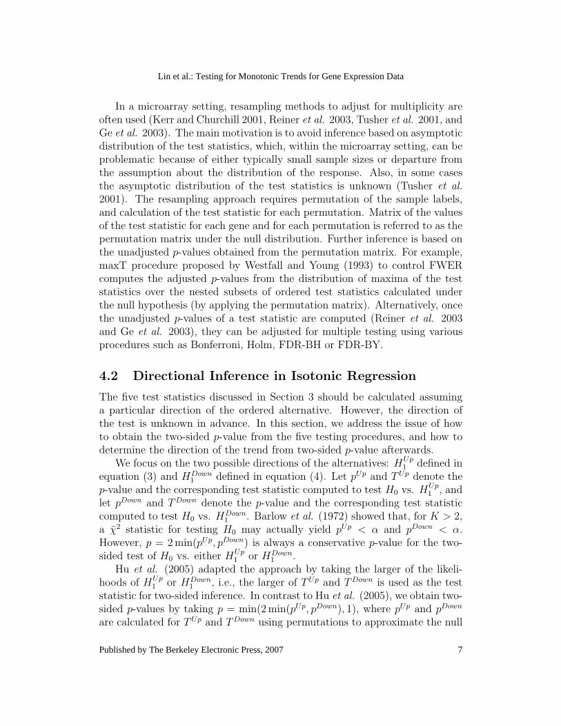
Table 1 shows the number of rejected hypotheses using several multiplicityadjusting methods and the five test statistics that are tested at the signif-icance level of 0.05. Figure 2 shows the adjusted p-values for the five teststatistics. Clearly, the adjusted p-values for maxT, Bonferroni, and FDR-BYare larger than the adjusted p-values obtained for FDR-BH. For instance, forE2

01, without adjusting for multiple testing, we reject the null hypothesis for5457 genes. With Bonferroni, Holm, and FDR-BY adjustment procedures weobtain the same number of significant genes, i.e., 1814. Using maxT for con-trolling FWER seems to be the most conservative approach with only 224genes declared significant.

Table 1: Number of rejected null hypotheses for various testing procedures atthe significance level of 0.05.

Method E201 Willams Marcus M Modified M

Unadjusted 5457 5238 5465 5449 5451maxT 224 215 223 265 251

Bonferroni 1814 1592 1669 1755 1745Holm 1814 1592 1669 1755 1745

FDR-BH 3613 3209 3533 3562 3567FDR-BY 1814 1592 1669 1755 1745

Note that the number of significant genes obtained for each test statistic fora given multiple testing adjustment is similar. For example, for the FDR-BHadjustment, we find 3613, 3562, and 3567 significant genes for E2

01, M , and themodified M statistic, respectively. This method yields more liberal results ascompared to the other multiple testing adjustment procedures. For that rea-son, FDR adjustment for multiplicity is commonly used within the microarrayframework (Ge et al. 2003, Tusher et al. 2001, Storey and Tibshirani 2003).Moreover, FDR-BH controls for the directional FDR (as discussed in Section4.3). Therefore, in what follows, we use FDR-BH procedure to investigate theperformance of the considered test statistics.

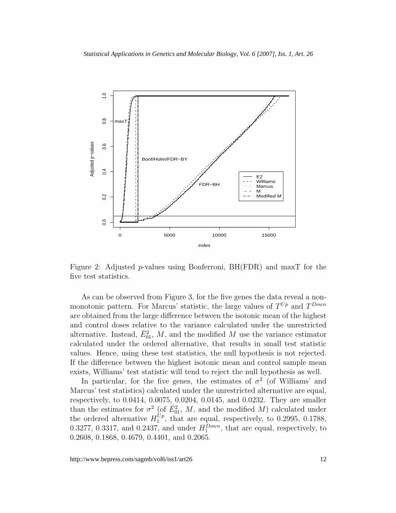
As we argue in Section 4.2, there is a possibility (although unlikely), thatthe null hypothesis is rejected for both directions (i.e., pUp ≤ α/2 and pDown ≤α/2). For the analysis discussed above, only five genes are rejected by Marcus’statistic with pUp and pDown smaller than the rejection threshold (with multipletesting adjustment), suggesting a non-monotonic trend. The five genes areshown in Figure 3.

11



0 5000 10000 15000

0.0

0.2

0.4

0.6

0.8

1.0

index

Adju

sted

p−v

alue

s

E2WilliamsMarcusMModified M

maxT

Bonf/Holm/FDR−BY

FDR−BH

Figure 2: Adjusted p-values using Bonferroni, BH(FDR) and maxT for thefive test statistics.

As can be observed from Figure 3, for the five genes the data reveal a non-monotonic pattern. For Marcus’ statistic, the large values of TUp and TDown

are obtained from the large difference between the isotonic mean of the highestand control doses relative to the variance calculated under the unrestrictedalternative. Instead, E2

01, M , and the modified M use the variance estimatorcalculated under the ordered alternative, that results in small test statisticvalues. Hence, using these test statistics, the null hypothesis is not rejected.If the difference between the highest isotonic mean and control sample meanexists, Williams’ test statistic will tend to reject the null hypothesis as well.

In particular, for the five genes, the estimates of σ2 (of Williams’ andMarcus’ test statistics) calculated under the unrestricted alternative are equal,respectively, to 0.0414, 0.0075, 0.0204, 0.0145, and 0.0232. They are smallerthan the estimates for σ2 (of E2

01, M , and the modified M) calculated underthe ordered alternative HUp

1 , that are equal, respectively, to 0.2995, 0.1788,0.3277, 0.3317, and 0.2437, and under HDown

1 , that are equal, respectively, to0.2608, 0.1868, 0.4679, 0.4401, and 0.2065.

12



1.0 2.0 3.0 4.0

6.9

7.0

7.1

7.2

7.3

7.4

dose

gene

exs

pres

sion

+

+

+

+*

* * ** * *

*

Gene: 200767_s_at

1.0 2.0 3.0 4.0

11.3

11.4

11.5

11.6

dose

gene

exs

pres

sion

+

+

+

+*

* * ** * *

*

Gene: 202483_s_at

1.0 2.0 3.0 4.0

11.2

11.3

11.4

11.5

11.6

11.7

11.8

dose

gene

exs

pres

sion +

+

+

+

* * *

*

*

** *

Gene: 211970_x_at

1.0 2.0 3.0 4.0

11.4

11.5

11.6

11.7

11.8

11.9

12.0

dose

gene

exs

pres

sion +

+

+

+

* * *

*

*

*

* *

Gene: 211983_x_at

1.0 2.0 3.0 4.0

11.3

11.4

11.5

11.6

11.7

dose

gene

exs

pres

sion

+

+

+

+

* * *

**

*

* *

Gene: 212988_x_at

Figure 3: Five genes rejected by Marcus’ statistics with both pUp and pDown

values smaller than the rejection threshold. Solid line: the isotonic meansobtained for testing H0 against HUp

1 . Dashed line: the isotonic means obtainedfor testing testing H0 against HDown

1 .

5.2 Comparison Between E201, M , and the Modified M

Test Statistics

Although in our case study, the number of significant genes obtained for thefive testing procedures is very similar, there are some discrepancies. In thissection, we investigate the subset of genes not commonly found by E2

01, M ,and the modified M statistics, respectively.

First we compare genes identified as significant or non-significant by M andE2

01. The logarithm of two-sided p-values for these genes is shown in Figure 4.Among the total of 16,998 genes, 3420 genes are found significant for monotonictrends for both statistics. However, 193 genes are found to be significant forE2

01 and non-significant for M -test statistic, while for 142 genes the reversedorder is observed. These genes account for 8.9% ((193+142)/(3420+193+142))of the total significant findings for both test statistics, which is not negligible.

13



−4 −3 −2 −1 0

−4−3

−2−1

0

Log (E2 p values)

Log

(M p

val

ues)

log (E2 p values) vs. log (M p values)

a

c

b

d

Figure 4: Logarithm of p-values (two sided) for E201 and M . Panel a: 3420

genes rejected by both E201 and M statistics; panel b: 142 genes are rejected

by M statistic only; panel c: 193 genes in are rejected from E201 only; panel d:

13,244 genes are not rejected by either statistic.

Similar to Hu et al. (2005), we compare the ranking of M and E201 of all the

genes. In both Hu et al. (2005) and our example the correlation of the ranks isequal to 0.99. Based on their observation, Hu et al. (2005) concluded that thetwo statistics perform similarly. However, in our data, the correlation of ranksof 142 genes found significant only for the M statistic (panel c of Figure 5) is0.92, while the correlation of ranks of 193 genes significant only for E2

01 (panelb) is 0.85. Both are somewhat lower than the correlation for genes in panel a(3420 genes significant for both statistics, correlation of 0.98) and in panel d(genes non-significant by either statistic, correlation of 0.99). The discrepantconclusions (rejecting the null only for one of statistic) can be explained bythe fact that the M statistic looks for the mean difference between the highestdose and the control. On the other hand, E2

01 is a global test for the monotonictrend.

The logarithm of the two sided p-values for the genes identified as sig-

14



11000 13000 15000 17000

1200

014

000

1600

0

rank M

rank

E

a

12000 13000 14000

1100

013

000

rank M

rank

E

b

11000 12000 13000 14000

1150

012

500

1350

014

500

rank M

rank

E

c

0 2000 6000 10000 14000

050

0010

000

1500

0

rank M

rank

E

d

Figure 5: Correlation between E201 and M . Panel a: correlation (0.98) between

rankings of 3420 genes rejected both from E201 and M . Panel b: correlation

(0.92) between rankings of 142 genes rejected only from M . Panel c: correla-tion (0.85) between rankings of 193 genes rejected only from E2

01 and Panel d:correlation (0.99) between rankings of 13,244 genes not rejected from E2

01 andM .

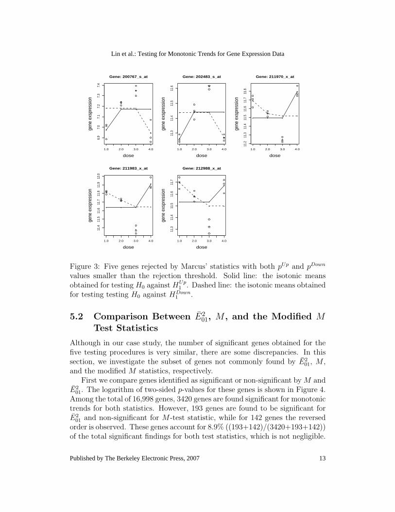
nificant or non-significant by the M and modified M statistics is shown inFigure 6. Among the total of 16,998 genes, 3478 genes are found signifi-cant for monotonic trends for both tests. However, 86 genes are found to besignificant for the M statistic and non-significant for the modified M test,while for 89 genes the reverse is true. These genes account for about 4.8%((86 + 89)/(86 + 89 + 3478)) of the total significant findings for both teststatistics.

The overall correlation between the ranks of genes obtained for M and themodified M test statistics is 0.99. The correlation between genes in each panelof Figure 7 is also very high, with 0.97 (in panel b) for genes rejected only bythe modified M , 0.98 (in panel c) for genes rejected only by M , 0.99 (in panela) for genes rejected by both of the test statistics, and 0.998 (in panel c) for

15



−4 −3 −2 −1 0

−4−3

−2−1

0

Log (M p values)

Log

(Mod

ified

M p

val

ues)

log (M p values) vs. log (Modified M p values)

a

c

b

d

Figure 6: Logarithm of p-values (two sided) for the M and the modified M .Panel a: 3478 genes are rejected by both M and the modified M statistics;panel b: 86 genes are rejected by M statistic only; panel c: 89 genes arerejected from the modified M only; panel d: 13,345 genes are not rejected byeither statistic.

genes rejected by neither of the test statistics. The difference between thetwo statistics lies in the adjustment of the degrees of freedom in the standarderror estimator of the modified M test statistic. Nevertheless, the discrepancyfound is not substantial.

6 Simulation Study

We conduct a simulation study to investigate the performance of the five teststatistics. In Section 6.1, we compare the three estimators for the variance ofWilliams’ and Marcus’ (which is the same), M , and modified M test statistics.In Section 6.2 we investigate the power of the five statistics for a single gene,while in Section 6.3, the power of the tests with the multiple testing adjustment

16



11000 13000 15000 17000

1100

013

000

1500

017

000

rank M

rank

Mod

ifed

M

a

11000 12000 13000 14000

1100

012

000

1300

014

000

rank M

rank

Mod

ifed

M

b

11000 12000 13000 14000 15000

1100

013

000

1500

0

rank M

rank

Mod

ifed

M

c

0 5000 10000 15000

040

0080

0012

000

rank M

rank

Mod

ifed

M

d

Figure 7: Correlation between M and the modified M . Panel a: correlation(0.99) between rankings of 3478 genes rejected both from M and the modifiedM . Panel b: correlation (0.97) between rankings of 89 genes rejected onlyfrom the modified M . Panel c: correlation (0.98) between rankings of 86genes rejected only from M and Panel d: correlation (0.998) between rankingsof 13,345 genes not rejected from the M and modified M .

is evaluated.

6.1 Standard Error Comparison

As a base for the simulations, the ANOVA model (1) is assumed. With fourdose levels, the order-restricted alternative hypothesis (3) can be classifiedinto seven possible trends. Table 2 defines the mean structure and assumedparameter values for these seven models, and for the null model (H0) used inthe simulations. The scale parameter λ controls the magnitude of the isotonicmeans. The larger λ, the larger distance between the means. In this set ofsimulations it is chosen to equal 1 and 3 based on the settings considered byMarcus (1976).

17



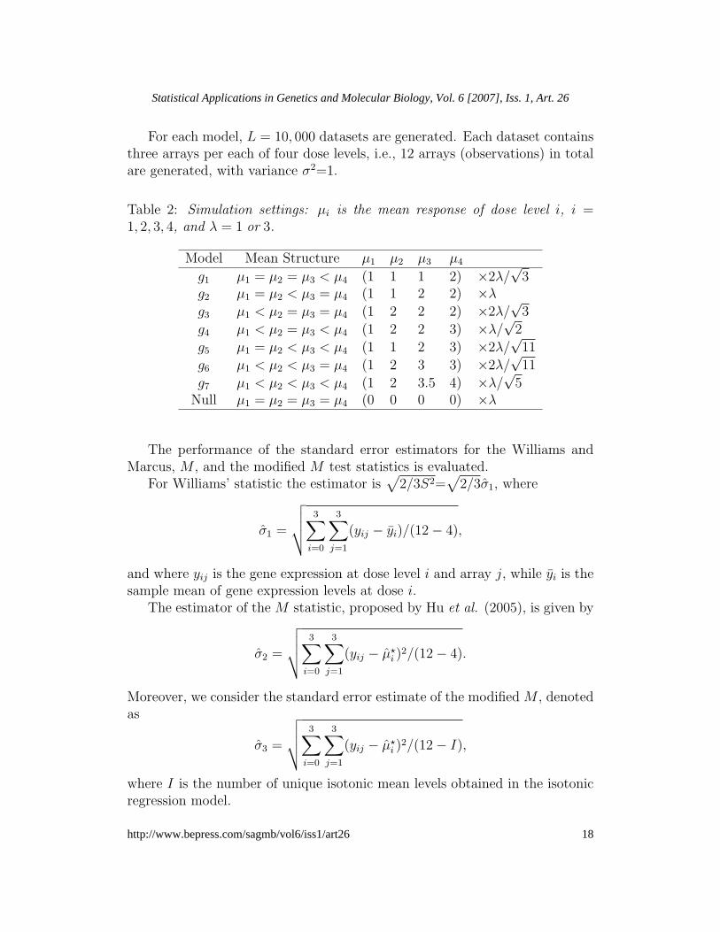
For each model, L = 10, 000 datasets are generated. Each dataset containsthree arrays per each of four dose levels, i.e., 12 arrays (observations) in totalare generated, with variance σ2=1.

Table 2: Simulation settings: µi is the mean response of dose level i, i =1, 2, 3, 4, and λ = 1 or 3.

Model Mean Structure µ1 µ2 µ3 µ4

g1 µ1 = µ2 = µ3 < µ4 (1 1 1 2) ×2λ/√

3g2 µ1 = µ2 < µ3 = µ4 (1 1 2 2) ×λ

g3 µ1 < µ2 = µ3 = µ4 (1 2 2 2) ×2λ/√

3

g4 µ1 < µ2 = µ3 < µ4 (1 2 2 3) ×λ/√

2

g5 µ1 = µ2 < µ3 < µ4 (1 1 2 3) ×2λ/√

11

g6 µ1 < µ2 < µ3 = µ4 (1 2 3 3) ×2λ/√

11

g7 µ1 < µ2 < µ3 < µ4 (1 2 3.5 4) ×λ/√

5Null µ1 = µ2 = µ3 = µ4 (0 0 0 0) ×λ

The performance of the standard error estimators for the Williams andMarcus, M , and the modified M test statistics is evaluated.

For Williams’ statistic the estimator is√

2/3S2=√

2/3σ1, where

σ1 =

√√√√3∑

i=0

3∑j=1

(yij − yi)/(12− 4),

and where yij is the gene expression at dose level i and array j, while yi is thesample mean of gene expression levels at dose i.

The estimator of the M statistic, proposed by Hu et al. (2005), is given by

σ2 =

√√√√3∑

i=0

3∑j=1

(yij − µ?i )

2/(12− 4).

Moreover, we consider the standard error estimate of the modified M , denotedas

σ3 =

√√√√3∑

i=0

3∑j=1

(yij − µ?i )

2/(12− I),

where I is the number of unique isotonic mean levels obtained in the isotonicregression model.

18



First, we evaluate the mean squared error (MSE) of σ1, σ2, and σ3. Thesquared bias is estimated by b2

σ = (¯σ−σ)2, with ¯σ =∑L

j=1 σj/L. The empirical

variance is estimated by vσ =∑L

j=1(σj − ¯σ)2/L, leading to the simulation

estimate of the MSE given by ˆMSEσ = b2σ + vσ.

Table 3 shows the squared bias, variance, and the MSE estimates of thethree standard error estimators under the null hypothesis and under the sevenalternative hypotheses. The smallest MSE values are obtained for σ3. Notethat although σ3 tends to have the highest squared bias, its mean square erroris the smallest due to the small variability of this estimator.

19



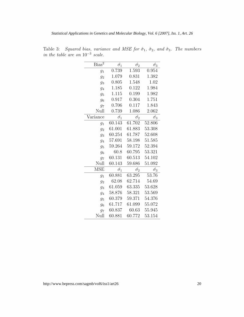
Table 3: Squared bias, variance and MSE for σ1, σ2, and σ3. The numbersin the table are on 10−3 scale.

Bias2 σ1 σ2 σ3

g1 0.739 1.593 0.954g2 1.079 0.831 1.382g3 0.805 1.548 1.02g4 1.185 0.122 1.984g5 1.115 0.199 1.982g6 0.917 0.304 1.751g7 0.706 0.117 1.843

Null 0.739 1.086 2.062Variance σ1 σ2 σ3

g1 60.143 61.702 52.806g2 61.001 61.883 53.308g3 60.254 61.787 52.608g4 57.691 58.198 51.585g5 59.264 59.172 52.394g6 60.8 60.795 53.321g7 60.131 60.513 54.102

Null 60.143 59.686 51.092MSE σ1 σ2 σ3

g1 60.881 63.295 53.76g2 62.08 62.714 54.69g3 61.059 63.335 53.628g4 58.876 58.321 53.569g5 60.379 59.371 54.376g6 61.717 61.099 55.072g7 60.837 60.63 55.945

Null 60.881 60.772 53.154

20



6.2 Power Study for a Single Gene Setting

Another simulation study is conducted to evaluate the power of the five teststatistics, for a single gene setting. Similarly, as in the study presented inSection 6.1, datasets of 12 arrays are generated under the seven order-restrictedmodels and the null model (Table 2). For each model (except for the nullmodel), 5000 datasets are generated with an increasing and a decreasing trend,respectively. For the null model, 10,000 datasets in total are simulated for thecomparison of the error rates. The isotonic means of the seven alternativesare specified in Table 2 with variance σ2 = 1.

For each dataset and each test, p-values are obtained from 10,000 per-mutations. The results are summarized by the proportion of significant tests(with permutation-based p-values ≤ 0.05) that correctly classify the increas-ing or decreasing trend. For each λ the power and Type I error are shownin Table 4. The standard error estimate of the power can be obtained by√

p(1− p)/10, 000 (Marcus 1976) where p is the estimate for the power.The estimated Type I error probability is around 5% for all the tests.

The power of the tests depends on the alternative. In general, regardingE2

01, Williams’ and Marcus’ tests, we arrive at the same conclusion as Marcus(1976), that the tests yield similar power. We can additionally observe thatM and the modified M tests perform similarly as the other three. Hence, fora single gene setting, no test is uniformly better than the others across the setof the considered alternative hypotheses.

6.3 Power Study Under Multiple Testing Adjustment

We have also investigated the power of the considered test statistics when deal-ing with the multiple testing problem. Micorarrays with 5000 genes per mi-croarray are generated. For each of the seven alternative models (see Table 2)a set of 100 genes (1400 genes in total) with an increasing and a decreasingtrend is included. For the remaining 3600 genes no dose effect is assumed (thenull model). The p-values for the considered test statistics are obtained using10,000 permutations, and the multiplicity adjustment is provided by using theFDR-BH procedure.

In total, 100 datasets are generated for settings with λ = 1 and λ = 3.Table 5 shows the power and FDR with their simulation-based standard errorestimates.

For λ = 1 the power of all the tests is very low. Moreover, FDR is notcontrolled at the desired level of 5%. This is related to the multiplicity ad-justment procedure: the total number of rejected hypothesis is small, and

21



Table 4: Power of the five test statistics for a single gene setting when dataare generated under the eight models in Table 2.

E201 Williams Marcus M Modified M

g1 0.2261 0.1882 0.2173 0.2299 0.1996g2 0.2772 0.2196 0.2404 0.2371 0.2331g3 0.2245 0.2189 0.199 0.2259 0.2096

λ = 1 g4 0.2602 0.2943 0.2706 0.3046 0.3177g5 0.3271 0.2684 0.2873 0.3134 0.301g6 0.2662 0.2454 0.2345 0.2604 0.2819g7 0.2953 0.2866 0.2744 0.3053 0.3231g1 0.9739 0.9369 0.961 0.9669 0.9169g2 0.9761 0.9058 0.9289 0.9462 0.887g3 0.9772 0.9773 0.9678 0.9773 0.9416

λ = 3 g4 0.9787 0.9914 0.9873 0.993 0.994g5 0.9871 0.9624 0.9761 0.9844 0.9822g6 0.9684 0.9706 0.9579 0.9747 0.9856g7 0.9803 0.9826 0.978 0.9883 0.9936

Null 0.0556 0.0584 0.0579 0.059 0.0564

Table 5: Power study of the five test statistics under multiple testing adjust-ment.

λ = 1 E201 Williams Marcus M Modified M

Power 0.0354 0.0287 0.0289 0.0306 0.0309SE(Power) (0.0049) (0.0046) (0.0046) (0.0048) (0.0048)FDR 0.1944 0.2077 0.2135 0.1835 0.1907Se(Power) (0.0507) (0.0579) (0.0568) (0.0534) (0.0534)λ = 3 E2

01 Williams Marcus M Modified MPower 0.9112 0.8454 0.8477 0.8905 0.8928SE(Power) (0.0074) (0.0099) (0.0096) (0.0082) (0.0079)FDR 0.0404 0.0424 0.0426 0.0399 0.0401SE(Power) (0.0053) (0.0054) (0.0053) (0.0052) (0.0052)

the proportion of wrong rejections is not well estimated, i.e, FDR is not wellcontrolled.

With λ = 3 the power of the test statistics is greatly improved and FDR

22



is well controlled. E201 seems to provide a slightly higher power compared to

the other tests. This can be explained by good performance in power underindividual seven models. Note that the power obtained using the modified Mtest statistic is comparable. When multiplicity is taken into account, E2

01, M ,and the modified M have higher power compared to Williams’ and Marcus’tests (0.9112, 0.8905, and 0.8928 compared to 0.8454 and 0.8477, respectively).

7 Discussion

In this paper, we evaluate several test statistics for testing monotonic trendin the relationship of gene expression and doses in a microarray context. Inparticular, we consider Williams’ step down procedure (Williams 1971, 1972),Marcus’ procedure (Marcus 1976), likelihood ratio statistic (Robertson et al.1988), M (Hu et al. 2005), and the modified M test statistic. Directional in-ference using these statistics is discussed for the situation when the directionof the trend is unknown in advance. To avoid inference based on asymp-totic theory, we consider the use of permutation tests. Accordingly, severalmultiplicity adjustment methods including directional FDR are applied. BHprocedure controlling FDR provides the most powerful approach as comparedto the other methods (Tusher et al. 2001, Ge et al. 2003, Storey and Tibshirani2003).

For the analysis discussed above, we observe comparable results for thefive test statistics. However, a difference in the results between M and E2

01

is observed. Modifying the number of degrees of freedom for the M statisticsimproves the MSE of the estimate of the standard error. However, the simula-tion study investigating power of the five test statistics under multiple testingadjustment shows that the M and the modified M have a similar power.

As we argue in Section 4.2, a two sided inference can result in rejecting thenull hypothesis in both directions (pUp < α/2 and pDown < α/2). This implies,as illustrated in Section 5.1, a non-monotone dose-response relationship. Thedifference between the four t-type test statistics (Williams’, Marcus’, M , andthe modified M) is due to the estimates of the standard error. Williams andMarcus used the unbiased estimator calculated under the unrestricted orderedalternative, while M and the modified M use an estimator calculated underthe ordered alternative. Williams’ and Marcus’ tests tend to reject geneswhen the difference calculated for the numerator exists and the standard errorcalculated under the unrestricted alternative is small. In particular, when thetrue means follow a simple tree (i.e., µ1 ≤ [µ2, µ3, µ4]), a unimodal partialordering (i.e., µ1 ≤ µ2 ≤ µ3 ≥ µ4) or a simple loop (i.e., µ1 ≤ [µ2, µ3] ≤ µ4)

23



(Robertson et al. 1988), Williams’ and Marcus’ tests are more likely to rejectthe null hypothesis of homogeneity of means (no dose effect) in favor of thesimple ordered alternative (HUp

1 or HDown1 ) than M and the modified M test

statistics. We have shown that for a single gene the power of the four t-typetest statistics is comparable (Table 4). However, the power after adjustingmultiplicity obtained for M and the modified M is higher than those obtainedfor Williams’ and Marcus’.

For a single gene the power obtained for E201 is comparable to the power

obtained for the four t-type test statistics. Moreover, after adjustment formultiplicity, the power obtained for E2

01 is only slightly higher than M and themodified M tests (shown in Table 5). In our opinion, if the question of primaryinterest is the comparison between the highest and the lowest dose levels, E2

01,M , and the modified M tests are comparable (in terms of FDR controlling andpower). However, if the question of primary interest is to detect a monotonetrend, the global test E2

01 is to be preferred.In this paper, we focus on testing the null hypothesis against a simple

ordered alternative. Whenever the null hypothesis is rejected, the primaryinterest is to identify the dose-response curve shape. For a dose-responseexperiment with K+1 dose levels, there is a finite number of isotonic modelswhich can be fitted to the data. For example, for an experiment with four doselevels there are seven upward monotone models (given in Table 2) and sevendownward monotone models, which can be fitted to the data. The testingprocedures discussed in this paper allows us to identify genes, for which thedose response curve is monotone, but not to identify the dose-response curveshape. The latter can be done using a model selection procedure, based oninformation criteria. Such a procedure will be presented in a future paper.

The R library implementing the methods presented in this paper is avail-able from the first author.

References

Affymetrix (2004) GeneChip Expression Analysis Technical Manual, Rev.4.Santa Clara, CA, available at http://www.affymetrix.com/support/tech-nical/manual/expression manual.affx.

Agresti, A. (1997) Statistical Methods for the Social Sciences, Finlay.

Barlow, R.E., Bartholomew, D.J., Bremner, M.J. and Brunk, H.D. (1972)Statistical Inference Under Order Restriction, New York: Wiley.

24



Bartholomew, D.J. (1961) Ordered tests in the analysis of variance, Biome-trika, 48, 325-332.

Benjamini, Y. and Hochberg, Y. (1995) Controlling the false discovery rate:a practical and powerful approach to multiple testing, J. R. Statist. Soc.B, 57, 289-300.

Benjamini Y. and Yekutieli, D. (2001) The control of the false discovery ratein multiple testing under dependency, ANN STAT, 29(4), 1165-1188.

Benjamini Y. and Yekutieli D. (2005a) False Discovery Rate-Adjusted Multi-ple Confidence Intervals for Selected Parameters, Journal of the AmericanStatistical Association, 100, 71-81.

Bolstad, B.M., Irizarry, R.A., Astrand, M. and Speed, T.P. (2002) A com-parison of normalization methods for high density oligonucleotide arraydata based on bias and variance.Bioinformatics,19, 185-193.

Chuang-Stein, C. and Agresti, A. (1997) Tutorial in biostatistics: A reviewof tests for detecting a monotone dose-response relationship with ordinalresponse data, Statistics in Medicine, 16, 2599-2618.

Ge, Y., Dudoit, S. and Speed, P.T. (2003) Resampling based multiple testingfor microarray data analysis, University of Berkeley, technical report 633.

Hochberg, Y. (1995) A sharper Bonferroni procedure for multiple tests ofsignificance, Biometrika, 75, 800–802.

Holm, S. (1979) A simple sequentially rejective multiple test procedure,Scand. J. Statist., 6, 65–70.

Hu, J., Kapoor, M., Zhang, W., Hamilton3, S.R., and Coombes1,K.R. (2005)Analysis of dose response effects on gene expression data with comparisonof two microarray platforms, Bioinformatics, 21(17), 3524–3529.

Hubbell, E., Liu, W.-M. and Mei. R. (2002) Robust estimators for expressionanalysis, Bioinformatics, 18(12), 1585-1592.

Kerr, M.K., Churchill, G.A. (2001) Statistical analysis of a gene expressionmicroarray experiment with replication, Biostatistics, 2, 183-201.

Marcus, R. (1976) The powers of some tests of the quality of normal meansagainst an ordered alternative, Biometrika, 63, 177-83.

25



Reiner, A., Yekutieli,D. and Benjamini,Y. (2003) Identifying differentiallyexpressed genes using false discovery rate controlling procedures. Bioin-formatics, 19(3), 368-375.

Robertson, T., Wright, F.T. and Dykstra, R.L. (1988), Order Restricted Sta-tistical Inference, Wiley.

Ruberg, S.J. (1995a) Dose response studies. I. Some design considerations,J. Biopharm. Stat., 5(1), 114.

Ruberg, S.J. (1995b) Dose response studies. II. Analysis and interpretation,J. Biopharm. Stat., 5(1), 1542.

Storey, JD and Tibshirani R. (2003) Statistical significance for genome-widestudies, Proceedings of the National Academy of Sciences, 100, 9440-9445.

Tusher, V.G., Tibshirani, R. and Chu, G. (2001) Significance analysis ofmicroarrys applied to the ionizing radiation response, PNAS, 98 , 5116-5121.

Westfall, P.H. and Young, S.S. (1993) Resampling Based Multiple Testing,Willy.

Williams, D.A. (1971) A test for differences between treatment means whenseveral dose levels are compared with a zero dose control, Biometrics, 27,103–117.

Williams, D.A. (1972) The comparision of several dose levels with a zero dosecontrol, Biometrics, 28, 519–531.

Yekutieli,D. and Benjamini,Y. (1999) Resampling-Based False Discovery RateControlling Multiple Test Procedures for Correlated Test Statistics, J.Stat. Plan. Infer., 82, 171-196.

26



Documents

Statistical Applications in Genetics and Molecular Biologyyekutiel/papers/SAGMB -- Dan Lin.pdf · Directional inference to testing ... Statistical Applications in Genetics and Molecular