Statistical Analysis

Professor Lynne Stokes

Department of Statistical Science

Lecture 15

Review

Brief Review

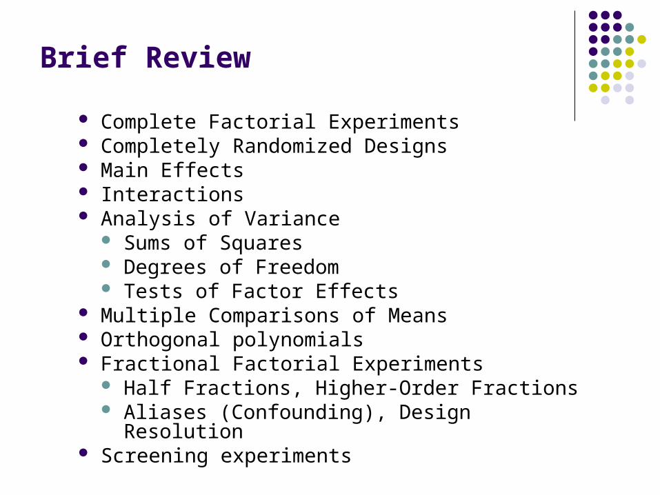
Complete Factorial Experiments Completely Randomized Designs Main Effects Interactions Analysis of Variance

Sums of Squares Degrees of Freedom Tests of Factor Effects

Multiple Comparisons of Means Orthogonal polynomials Fractional Factorial Experiments

Half Fractions, Higher-Order Fractions Aliases (Confounding), Design Resolution

Screening experiments

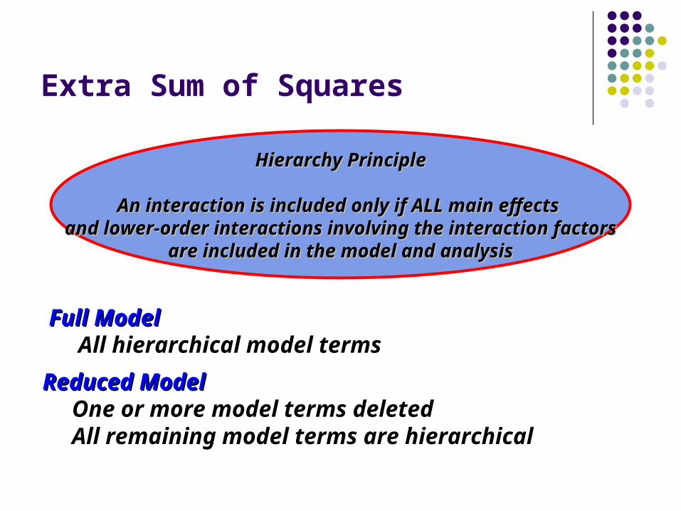
Extra Sum of Squares

Hierarchy PrincipleHierarchy Principle

An interaction is included only if ALL main effects An interaction is included only if ALL main effects and lower-order interactions involving the interaction factorsand lower-order interactions involving the interaction factors

are included in the model and analysisare included in the model and analysis

Full ModelFull Model All hierarchical model terms

Reduced ModelReduced Model One or more model terms deleted All remaining model terms are hierarchical

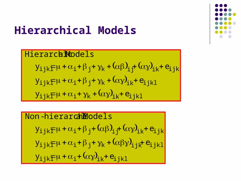
Hierarchical Models

ey

ey

ey

Models alHierarchic

ijklikkiijkl

ijklikkjiijkl

ijklikijkjiijkl

ey

ey

ey

Models alhierarchic-Non

ijklikiijkl

ijklijkkjiijkl

ijklikijjiijkl

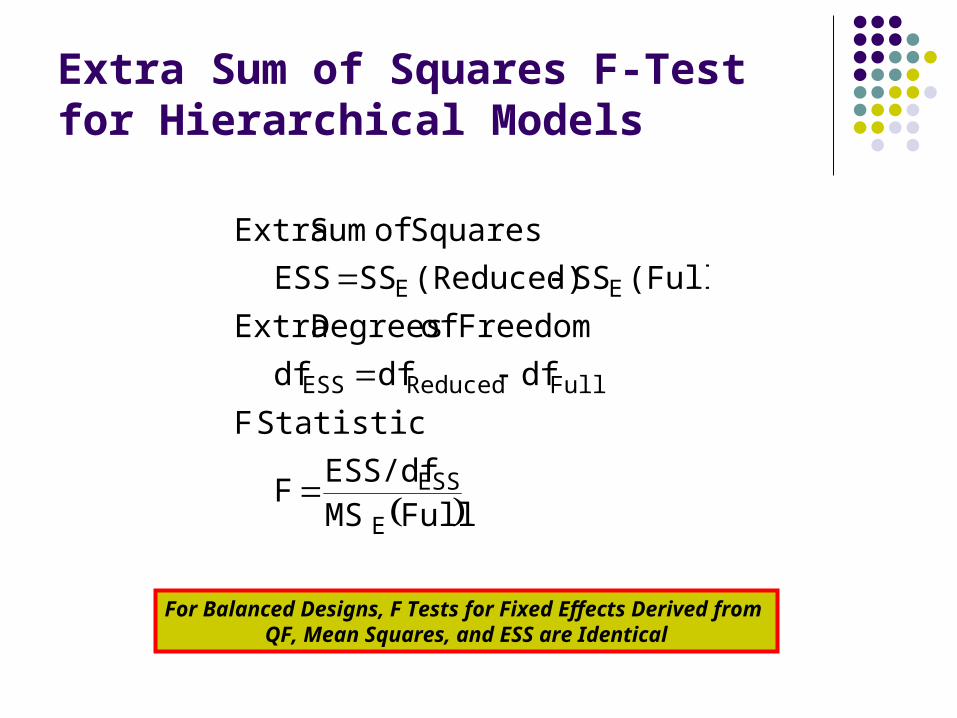
Extra Sum of Squares F-Testfor Hierarchical Models

FullMS

ESS/dfF

Statistic F

dfdfdf

Freedom of Degrees Extra

(Full)SS(Reduced)SSESS

Squares of Sum Extra

E

ESS

FullReducedESS

EE

For Balanced Designs, F Tests for Fixed Effects Derived from QF, Mean Squares, and ESS are Identical

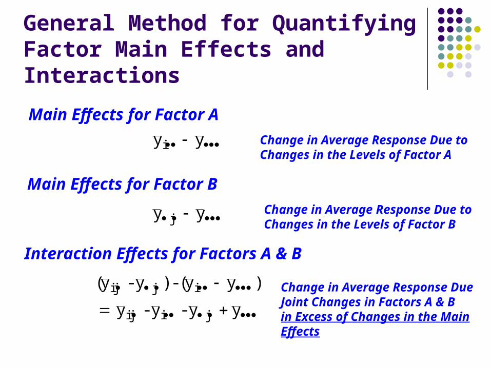
General Method for Quantifying Factor Main Effects and Interactions

Main Effects for Factor A

Main Effects for Factor B

Interaction Effects for Factors A & B

y i y

y j y

(y - y ) - (y

y - y - y

ij

ij i

j i

j

y

y

)

Change in Average Response Due toChanges in the Levels of Factor A

Change in Average Response Due toChanges in the Levels of Factor B

Change in Average Response DueJoint Changes in Factors A & Bin Excess of Changes in the MainEffects

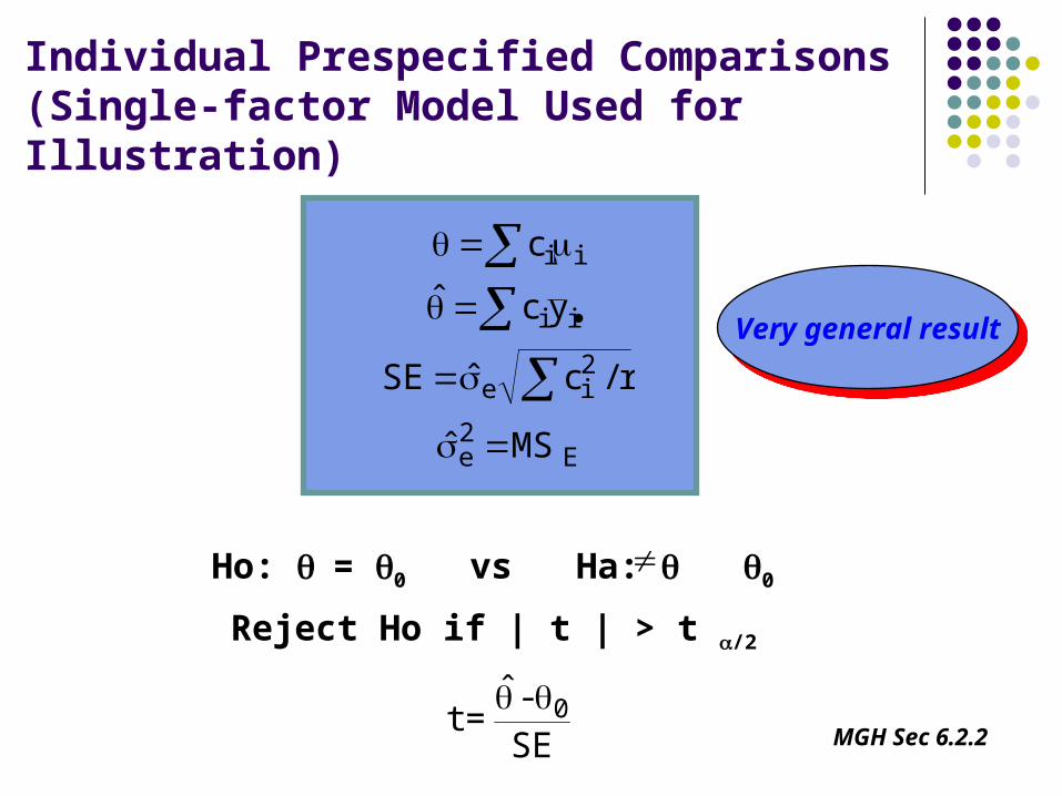
Individual Prespecified Comparisons(Single-factor Model Used for Illustration)

E2e

2ie

ii

ii

MSˆ

r/cˆSE

ycˆ

c

Ho: = 0 vs Ha: 0

Reject Ho if | t | > t /2

SE

-ˆ=t 0

Very general resultVery general result

MGH Sec 6.2.2

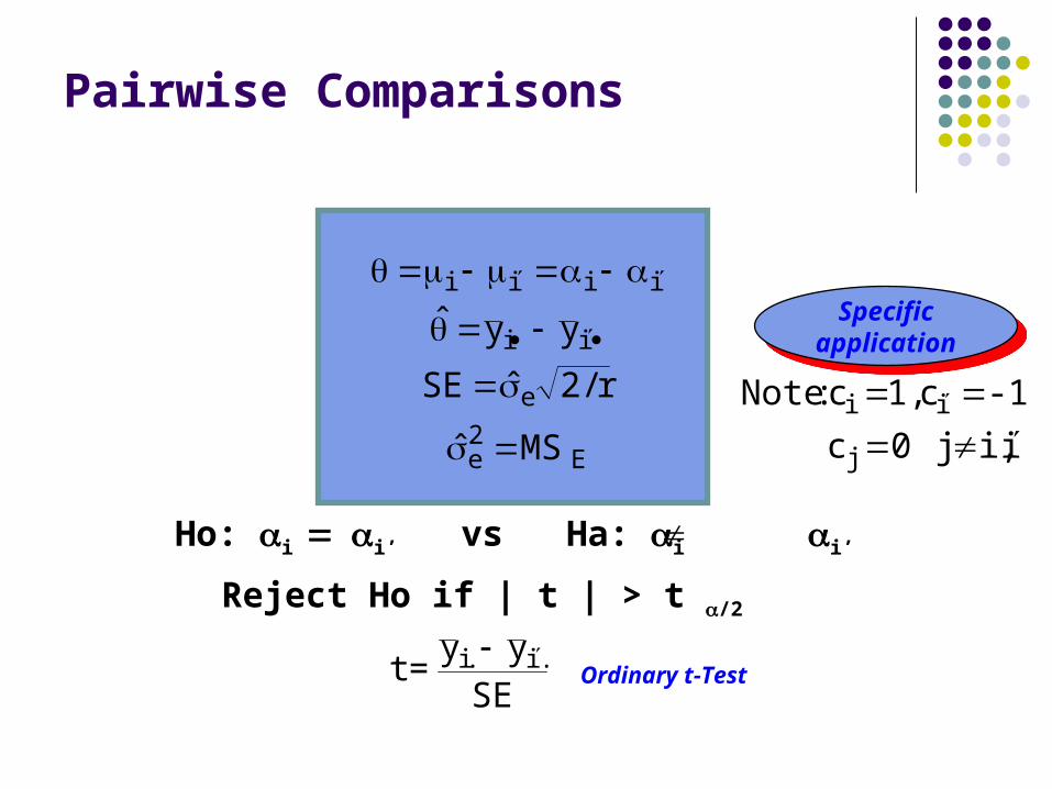
Pairwise Comparisons

E2e

e

ii

iiii

MSˆ

r/2ˆSE

yyˆ

Specific

application

Specificapplication

ii,j 0c

-1,c 1,c :Note

j

ii

Ho: i i’ vs Ha: ii’

Reject Ho if | t | > t /2

SE

yy=t .i.i

Ordinary t-Test

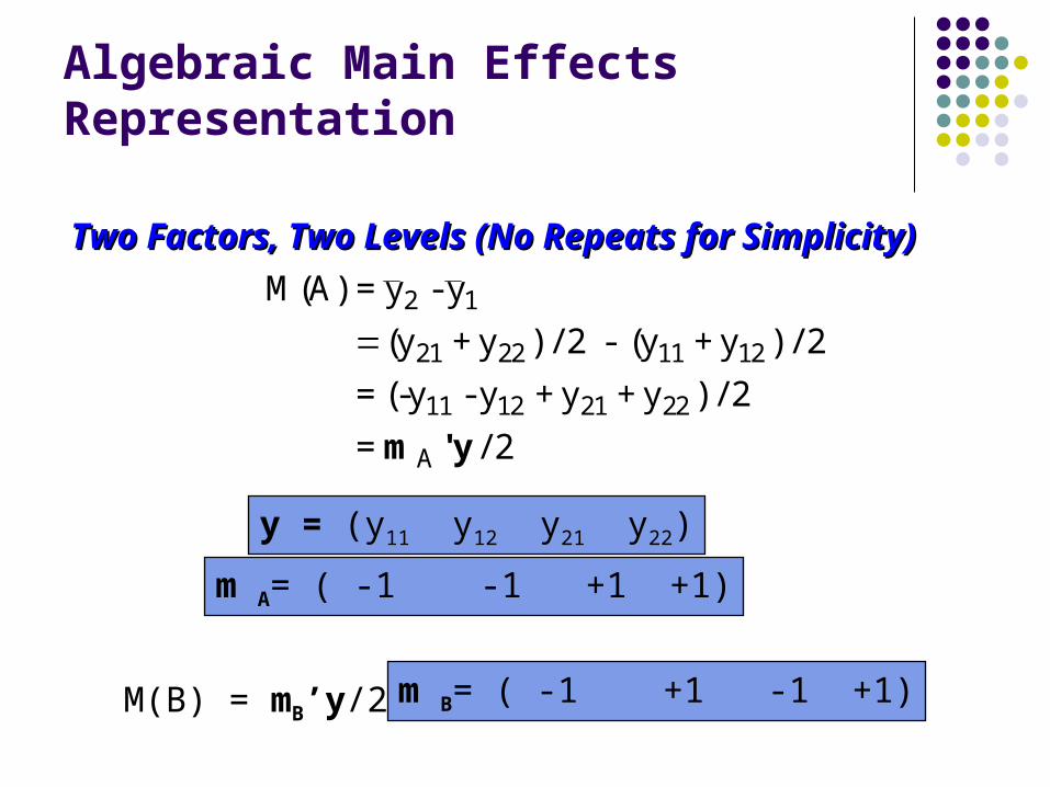
Algebraic Main Effects Representation

M(A) = y - y

(y + y ) / 2 - (y + y ) / 2

= (-y - y + y + y ) / 2

= / 2

2 1

21 22 11 12

11 12 21 22

A

m 'y

y = (y11 y12 y21 y22)

m A= ( -1 -1 +1 +1)

M(B) = mB’y/2 m B= ( -1 +1 -1 +1)

Two Factors, Two Levels (No Repeats for Simplicity)Two Factors, Two Levels (No Repeats for Simplicity)

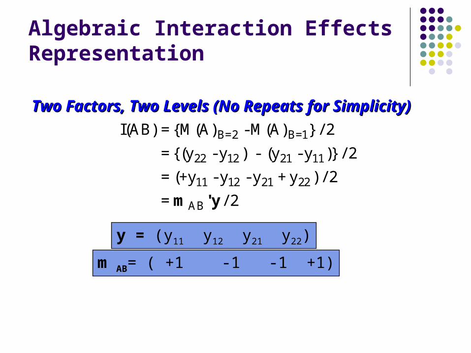
Algebraic Interaction Effects Representation

I(AB) = {M(A) - M(A)

= {(y - y ) - (y - y )} / 2

= (+y - y - y + y ) / 2

= / 2

B=2 B=1

22 12 21 11

11 12 21 22

AB

} / 2

m 'y

y = (y11 y12 y21 y22)

m AB= ( +1 -1 -1 +1)

Two Factors, Two Levels (No Repeats for Simplicity)Two Factors, Two Levels (No Repeats for Simplicity)

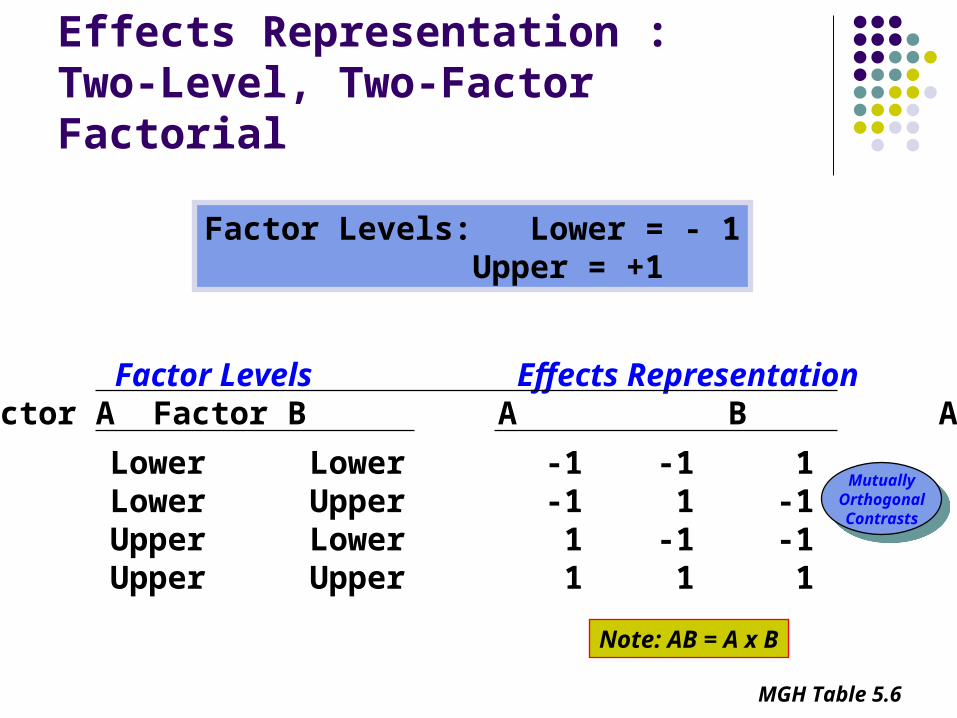
Effects Representation :Two-Level, Two-Factor Factorial

Factor Levels: Lower = - 1 Upper = +1

Factor Levels Effects RepresentationFactor A Factor B A B AB

LowerLowerUpperUpper

LowerUpperLowerUpper

-1-1 1 1

-1 1-1 1

1-1-1 1

Note: AB = A x B

MGH Table 5.6

MutuallyOrthogonalContrasts

MutuallyOrthogonalContrasts

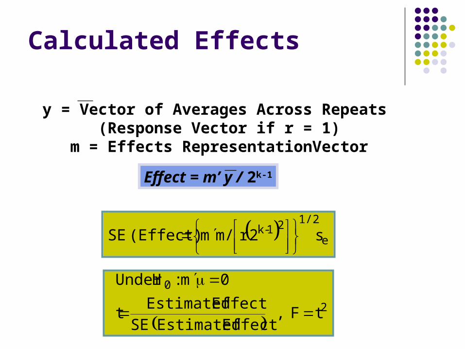
Calculated Effects

y = Vector of Averages Across Repeats (Response Vector if r = 1)

m = Effects RepresentationVector

Effect = m’ y / 2k-1

s2rm/m(Effect) SE e

1/221-k

tF ,

Effect Estimated SEEffect Estimated

t

0m:H Under

2

0

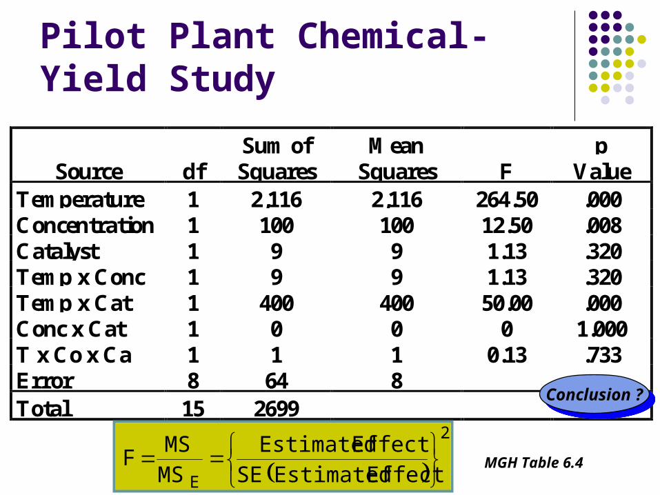
Pilot Plant Chemical-Yield Study

MGH Table 6.4

Source dfSum ofSquares

MeanSquares F

pValue

Temperature 1 2,116 2,116 264.50 .000Concentration 1 100 100 12.50 .008Catalyst 1 9 9 1.13 .320Temp x Conc 1 9 9 1.13 .320Temp x Cat 1 400 400 50.00 .000Conc x Cat 1 0 0 0 1.000T x Co x Ca 1 1 1 0.13 .733Error 8 64 8Total 15 2699 Conclusion ?Conclusion ?

2

E Effect Estimated SEEffect Estimated

MSMS

F

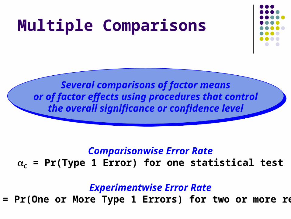
Multiple Comparisons

Several comparisons of factor meansor of factor effects using procedures that control

the overall significance or confidence level

Several comparisons of factor meansor of factor effects using procedures that control

the overall significance or confidence level

Comparisonwise Error RateC = Pr(Type 1 Error) for one statistical test

Experimentwise Error RateE = Pr(One or More Type 1 Errors) for two or more rests

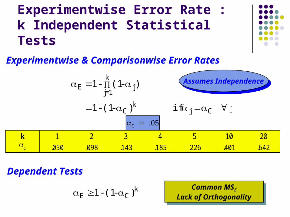
Experimentwise Error Rate :k Independent Statistical Tests

j if ) - (1 - 1

) - (1 - 1

Cjk

C

k

1=jjE

Experimentwise & Comparisonwise Error Rates

k 1 2 3 4 5 10 20

E .050 .098 .143 .185 .226 .401 .642

Dependent Tests

kCE ) - (1 - 1 Common MSE

Lack of Orthogonality

Common MSE

Lack of Orthogonality

C

Assumes IndependenceAssumes Independence

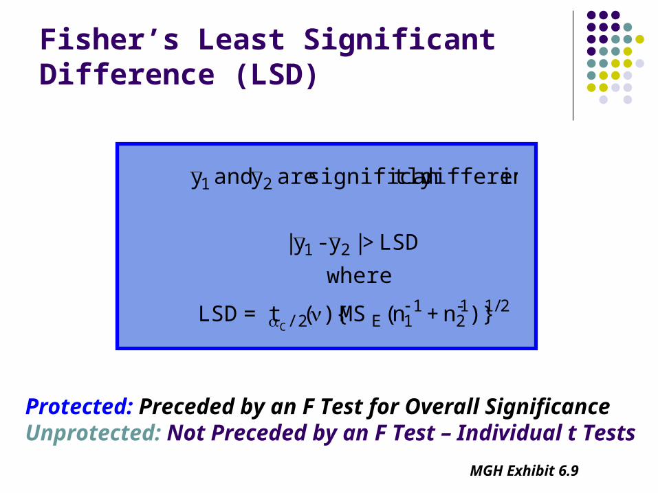
Fisher’s Least Significant Difference (LSD)

2/11-2

11E/2

21

21

)}n + n(MS){( t= LSD

where

LSD > | y - y |

ifdifferent tly significan are y and y

C

Protected: Preceded by an F Test for Overall SignificanceUnprotected: Not Preceded by an F Test – Individual t Tests

MGH Exhibit 6.9

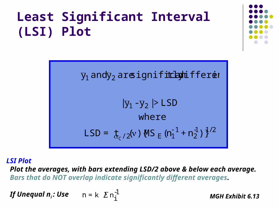
Least Significant Interval (LSI) Plot

2/11-2

11E/2

21

21

)}n + n(MS){( t= LSD

where

LSD > | y - y |

ifdifferent tly significan are y and y

C

LSI Plot Plot the averages, with bars extending LSD/2 above & below each average. Bars that do NOT overlap indicate significantly different averages.

If Unequal ni : Use 1-ink / =n MGH Exhibit 6.13

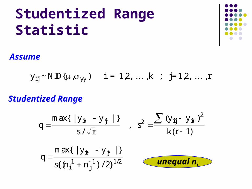
Studentized Range Statistic

Assume

y i = 1,2, . . . ,k ; j= 1,2, . . . , rij ~ { , )NID yy

Studentized Range

qy y

k rij i

max{ ( )

( )

| y - y | }

s / r , s

i j 22

1

qn j

max{

) / } /

| y - y | }

s{(n

i j

i-1 1 1 22 unequal ni

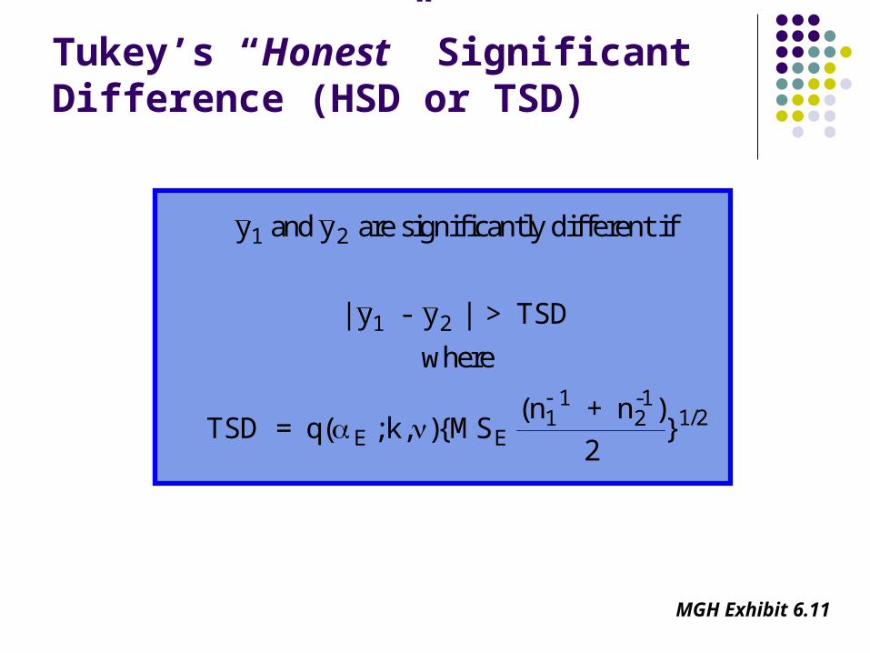
Tukey’s “Honest” Significant Difference (HSD or TSD)

y and y are significantly different if

| y - y | > TSD

where

TSD = q + n

1 2

1 2

2-1

( ; , ){( )

} / E Ek MSn1

11 2

2

MGH Exhibit 6.11

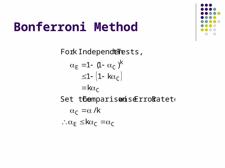
Bonferroni Method

CCE

C

C

C

kCE

k

k/

toRateError wiseComparison Set the

k

k11

)1(1

Tests,t Independenk For

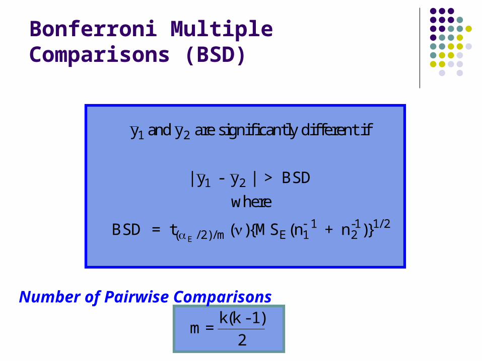
Bonferroni Multiple Comparisons (BSD)

y and y are significantly different if

| y - y | > BSD

where

BSD = t + n

1 2

1 2

2-1

E( / )//( ){ ( )} 2 1

1 1 2m EMS n

Number of Pairwise Comparisons

m =k(k - 1)

2

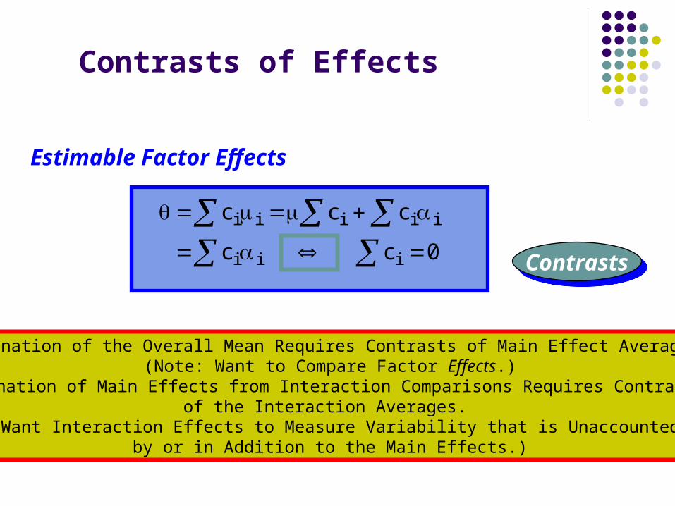
Contrasts of Effects

c c c

c

i i i i i

i i c i 0

Estimable Factor Effects

ContrastsContrasts

Elimination of the Overall Mean Requires Contrasts of Main Effect Averages.(Note: Want to Compare Factor Effects.)

Elimination of Main Effects from Interaction Comparisons Requires Contrasts of the Interaction Averages.

(Note: Want Interaction Effects to Measure Variability that is Unaccounted for by or in Addition to the Main Effects.)

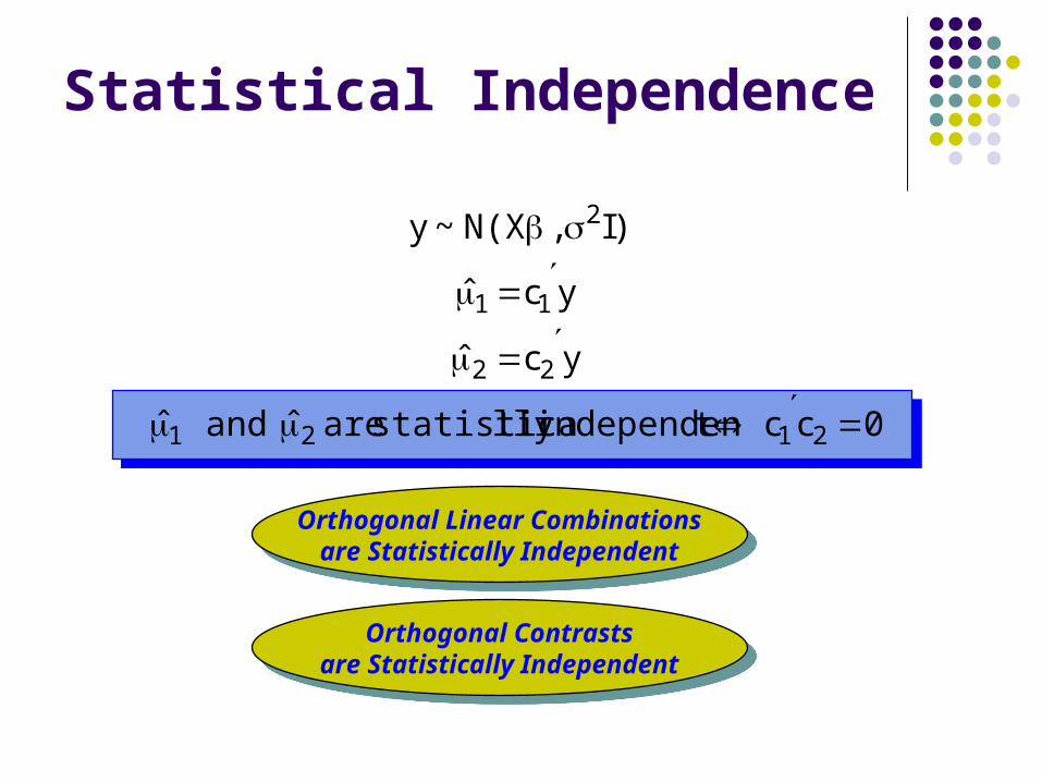
Statistical Independence

0cc t independenlly statistica are ˆ and ˆ

ycˆ

ycˆ

)I , N(X~y

2121

22

11

2

Orthogonal Linear Combinationsare Statistically Independent

Orthogonal Linear Combinationsare Statistically Independent

Orthogonal Contrastsare Statistically Independent

Orthogonal Contrastsare Statistically Independent

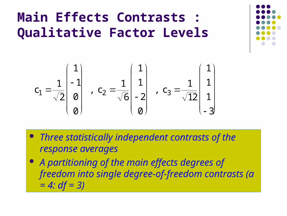
Main Effects Contrasts :Qualitative Factor Levels

c , c , c1 2 3

1

2

1

1

0

0

1

6

1

1

2

0

1

12

1

1

1

3

Three statistically independent contrasts of the response averages

A partitioning of the main effects degrees of freedom into single degree-of-freedom contrasts (a = 4: df = 3)

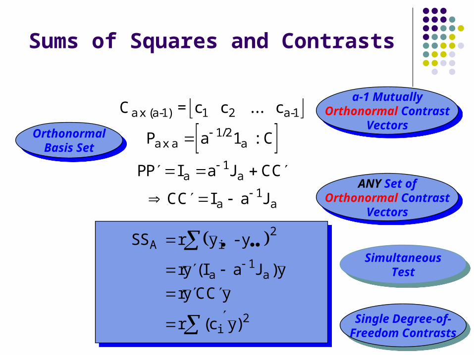
Sums of Squares and Contrasts

SS y - yA i

r

ry I a J y

ry CC y

r c y

a a

i

2

1

2

( )

( ) Single Degree-of-Freedom Contrasts

Single Degree-of-Freedom Contrasts

SimultaneousTest

SimultaneousTest

C = c c ... c

P : C

a x (a-1) 1 2 a-1

a x a

a

PP I a J CC

CC I a J

a

a a

a a

1 2

1

1

1/

a-1 MutuallyOrthonormal Contrast

Vectors

a-1 MutuallyOrthonormal Contrast

VectorsOrthonormal

Basis Set

OrthonormalBasis Set

ANY Set ofOrthonormal Contrast

Vectors

ANY Set ofOrthonormal Contrast

Vectors

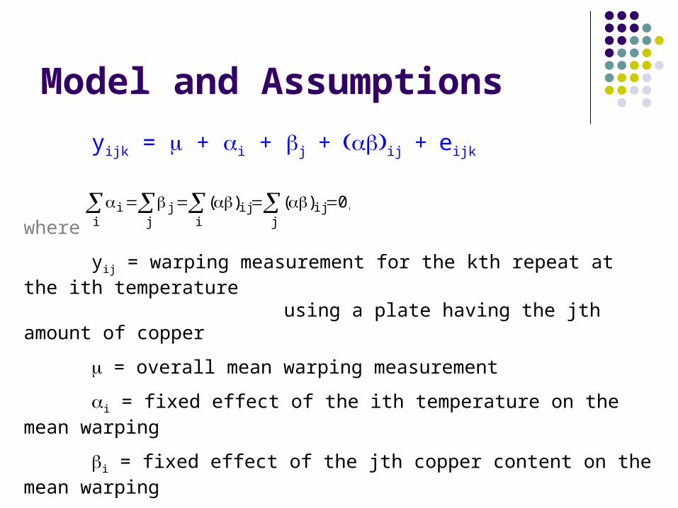
yijk = + i + j+ij+eijk

where

yij = warping measurement for the kth repeat at the ith temperature using a plate having the jth amount of copper

= overall mean warping measurement

i = fixed effect of the ith temperature on the mean warping

i = fixed effect of the jth copper content on the mean warping

(ij = fixed effect of the interaction between the ith temperature and the jth copper content on the mean warping

eij = random experimental error, NID(0,2)

Model and Assumptions

,0)()(j

iji

ijj

ji

i

Warping of Copper Plates

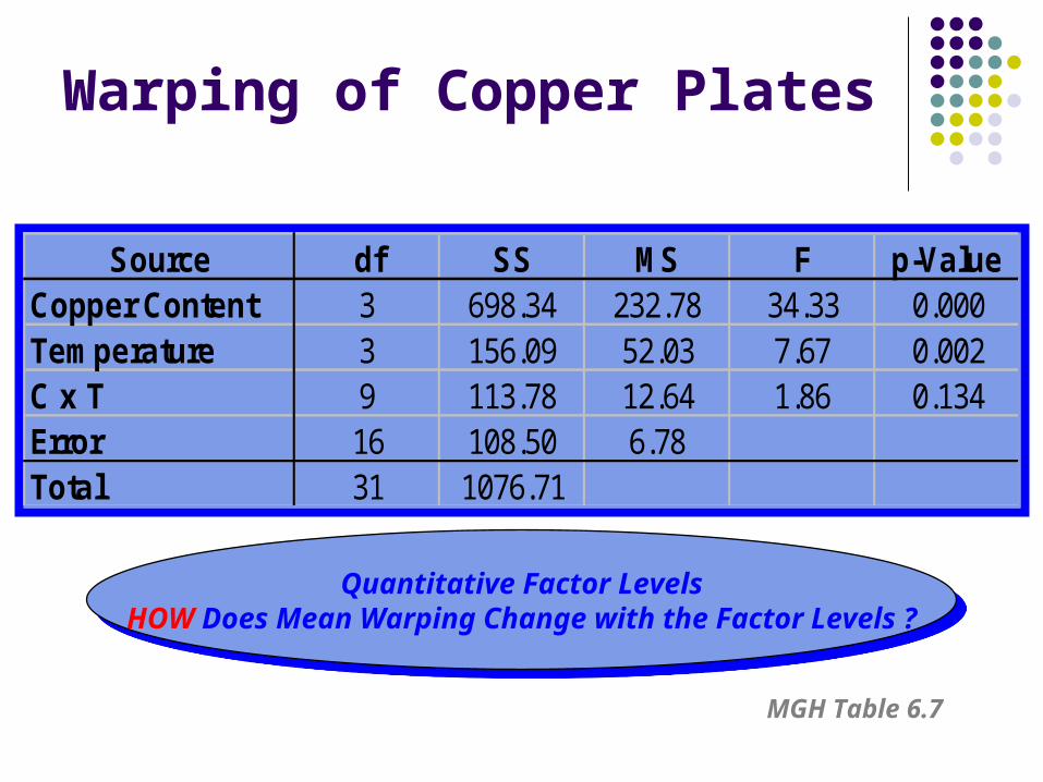
Source df SS MS F p-ValueCopper Content 3 698.34 232.78 34.33 0.000Temperature 3 156.09 52.03 7.67 0.002C x T 9 113.78 12.64 1.86 0.134Error 16 108.50 6.78Total 31 1076.71

MGH Table 6.7

Quantitative Factor LevelsHOW Does Mean Warping Change with the Factor Levels ?

Quantitative Factor LevelsHOW Does Mean Warping Change with the Factor Levels ?

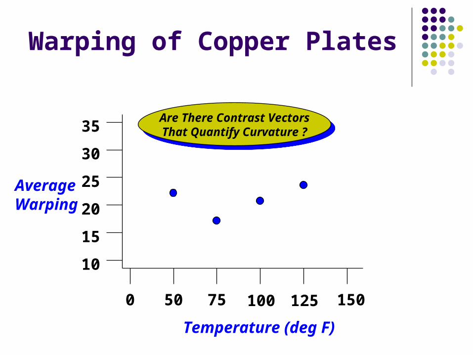
Warping of Copper Plates

0 50 75 100 125 150

Temperature (deg F)

10

15

20

25

30

35

AverageWarping

Are There Contrast VectorsThat Quantify Curvature ?

Are There Contrast VectorsThat Quantify Curvature ?

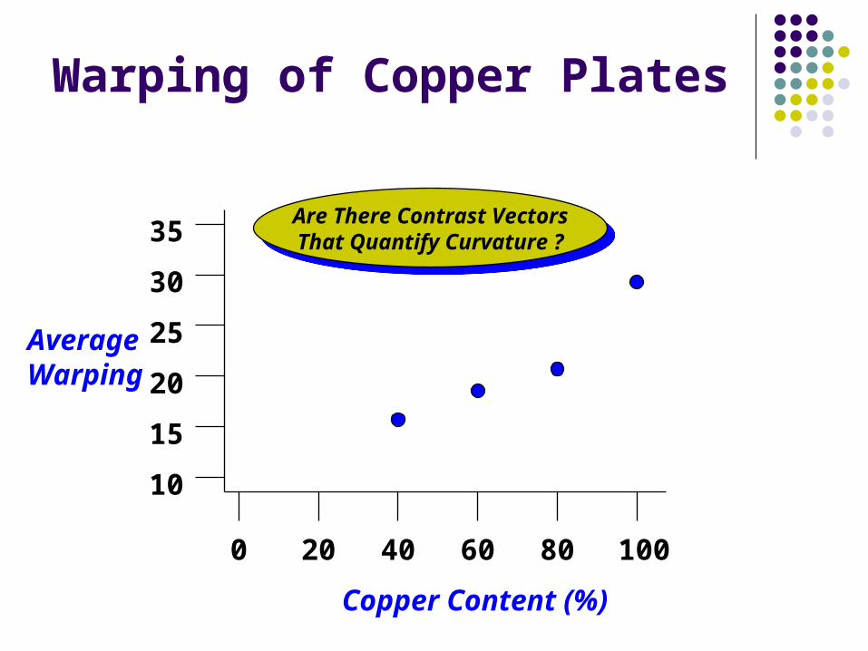
Warping of Copper Plates

0 20 40 60 80 100

Copper Content (%)

10

15

20

25

30

35

AverageWarping

Are There Contrast VectorsThat Quantify Curvature ?

Are There Contrast VectorsThat Quantify Curvature ?

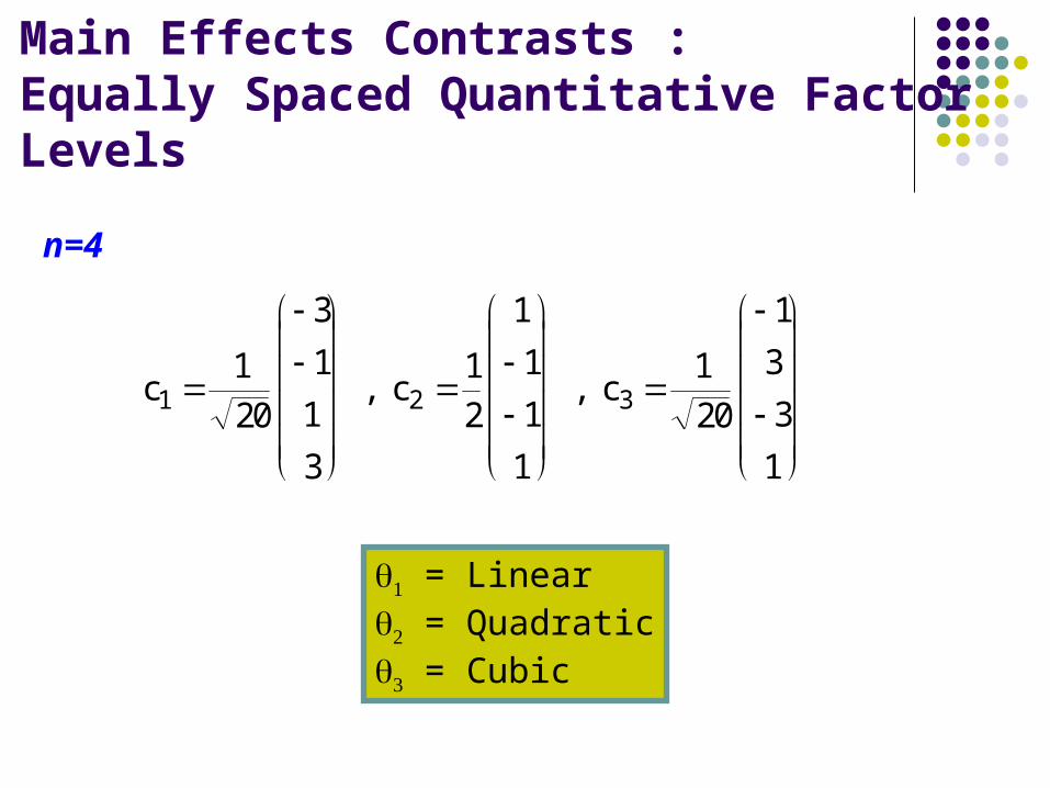
Main Effects Contrasts :Equally Spaced Quantitative Factor Levels

c , c , c1 2 3

1

20

3

1

1

3

1

2

1

1

1

1

1

20

1

3

3

1

= Linear = Quadratic = Cubic

n=4

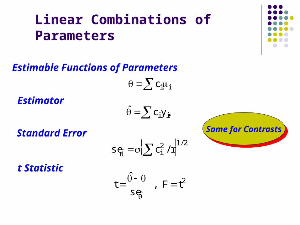
Linear Combinations of Parameters

Estimable Functions of Parameters

iic

Estimator

Standard Error

iiycˆ

2/12iˆ r/cse

t Statistic 2

ˆtF ,

se

ˆt

Same for ContrastsSame for Contrasts

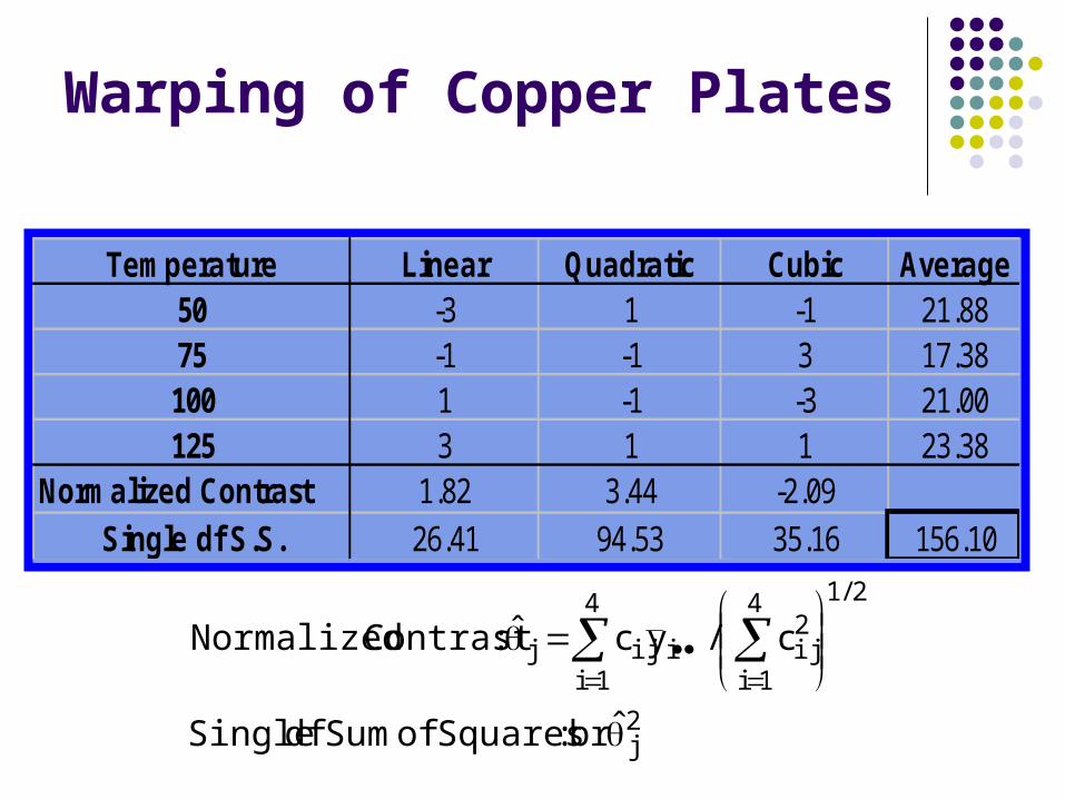
Warping of Copper Plates

Temperature Linear Quadratic Cubic Average50 -3 1 -1 21.8875 -1 -1 3 17.38100 1 -1 -3 21.00125 3 1 1 23.38

Normalized Contrast 1.82 3.44 -2.09Single df S.S. 26.41 94.53 35.16 156.10

2j

2/14

1i

4

1i

2ijiijj

ˆbr :Squares of Sum df Single

c/ycˆ :Contrast Normalized

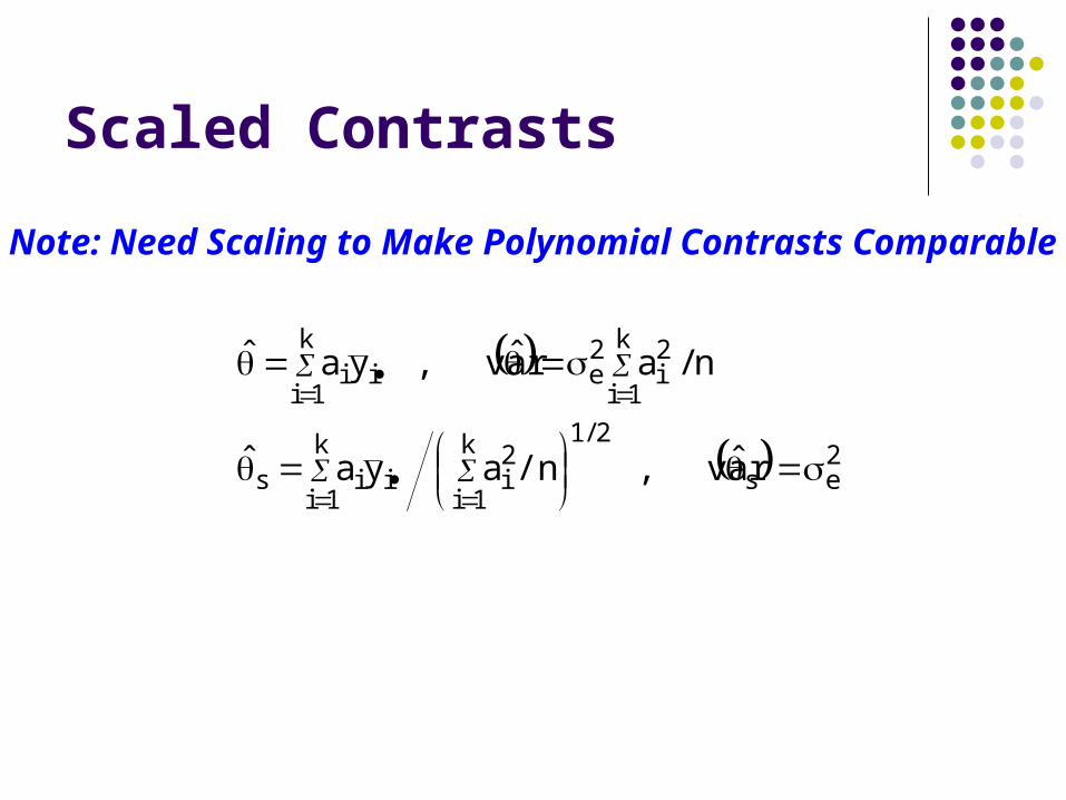
Scaled Contrasts

Note: Need Scaling to Make Polynomial Contrasts Comparable

2es

2/1k

1i

2i

k

1iiis

k

1i

2i

2e

k

1iii

ˆ var, /n ayaˆ

n/aˆ var, yaˆ

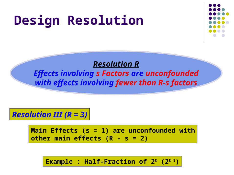
Design Resolution

Resolution REffects involving s Factors are unconfoundedwith effects involving fewer than R-s factors

Resolution III (R = 3)

Main Effects (s = 1) are unconfounded withother main effects (R - s = 2)

Example : Half-Fraction of 23 (23-1)

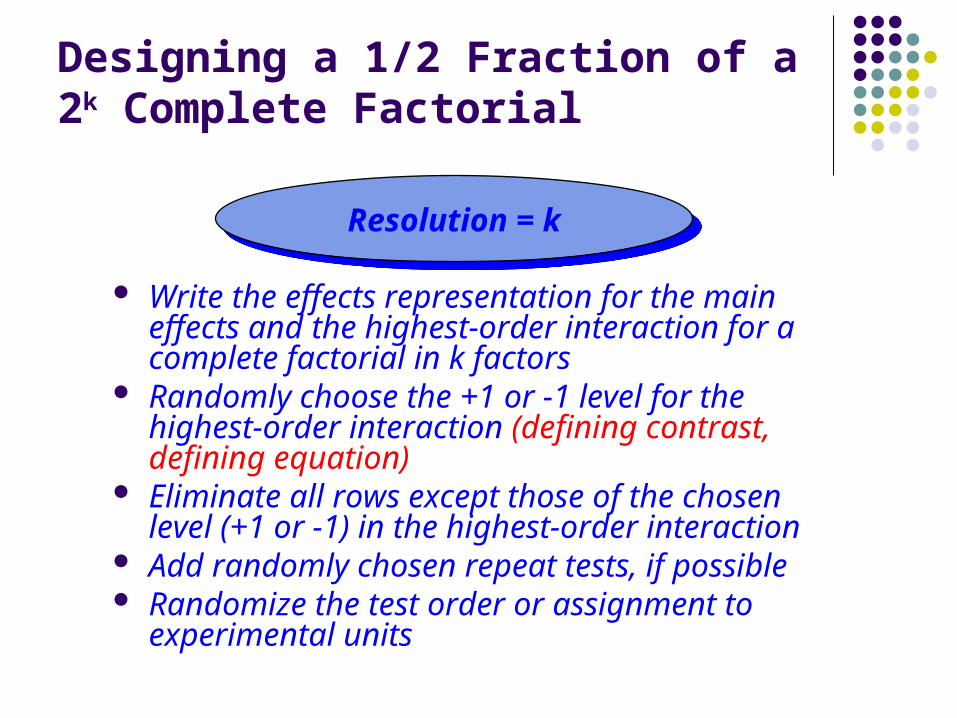
Designing a 1/2 Fraction of a 2k Complete Factorial

Write the effects representation for the main effects and the highest-order interaction for a complete factorial in k factors

Randomly choose the +1 or -1 level for the highest-order interaction (defining contrast, defining equation)

Eliminate all rows except those of the chosen level (+1 or -1) in the highest-order interaction

Add randomly chosen repeat tests, if possible Randomize the test order or assignment to

experimental units

Resolution = kResolution = k

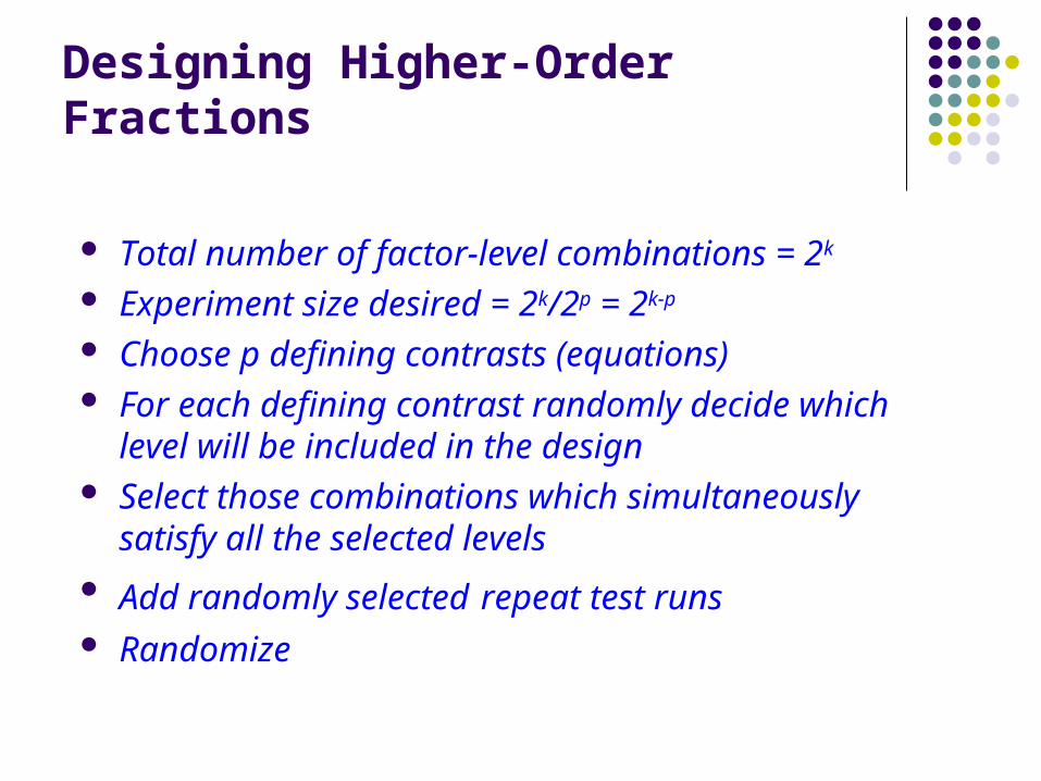
Designing Higher-Order Fractions

Total number of factor-level combinations = 2k

Experiment size desired = 2k/2p = 2k-p

Choose p defining contrasts (equations) For each defining contrast randomly decide which

level will be included in the design Select those combinations which simultaneously

satisfy all the selected levels Add randomly selected repeat test runs Randomize

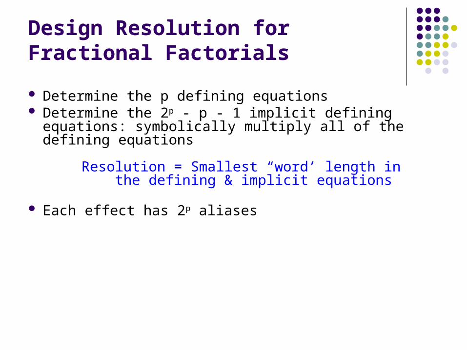
Design Resolution for Fractional Factorials

Determine the p defining equations Determine the 2p - p - 1 implicit defining equations:

symbolically multiply all of the defining equations

Resolution = Smallest “word’ length in the defining & implicit equations

Each effect has 2p aliases

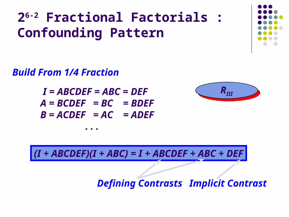
26-2 Fractional Factorials :Confounding Pattern

Build From 1/4 Fraction

I = ABCDEF = ABC = DEFA = BCDEF = BC = BDEFB = ACDEF = AC = ADEF . . .

RIIIRIII

(I + ABCDEF)(I + ABC) = I + ABCDEF + ABC + DEF

Defining ContrastsImplicit Contrast

26-2 Fractional Factorials :Confounding Pattern

Build From 1/2 Fraction

I = ABCDEF = ABC = DEFA = BCDEF = BC = BDEFB = ACDEF = AC = ADEF . . .

RIIIRIII

Optimal 1/4 Fraction

I = ABCD = CDEF = ABEFA = BCD = ACDEF = BEFB = ACD = BCDEF = AEF . . .

RIVRIV

Screening Experiments

Very few test runs Ability to assess main effects only Generally leads to a comprehensive

evaluation of a few dominant factors Potential for bias

Highly effective for isolating vital few strong effectsshould be used ONLY under the proper circumstancesHighly effective for isolating vital few strong effects

should be used ONLY under the proper circumstances

Plackett-Burman Screening Designs

Any number of factors, each having 2 levels Interactions nonexistent or negligible Relative

to main effectsNumber of test runs is a multiple of 4 At least 6 more test runs than factors should

be used

Fold-Over Designs

Reverse the signs on one or more factorsRun a second fraction with the sign reversalsUse the confounding pattern of the original

and the fold-over design to determine the alias structure Averages Half-Differences