Statistical analysis of strong-motion accelerograms and its

Geophys. J. Int. (1997) 129,113-123

Statistical analysis of strong-motion accelerograms and its application to earthquake early-warning systems

Gunnar Grecksch and Hans-Joachim Kumpel Geological Institute, Section of Applied Geophysics, University of Bonn, Nussallee 8, 0-531 15 Bonn, Germany

Accepted 1996 November 18. Received 1996 November 18; in original form 1996 August 13

SUMMARY In view of increasing damage due to earthquakes, and the current problems of earthquake prediction, real-time warning of strong ground motion is attracting more interest. In principle, it allows short-term warning of earthquakes while they are occurring. With warning times of up to tens of seconds it is possible to send alerts to potential areas of strong shaking before the arrival of the seismic waves and to mitigate the damage, but only if the seismic source parameters are determined rapidly. The major problem of an early-warning system is the real-time estimation of the earthquake’s size.

We investigated digitized strong-motion accelerograms from 244 earthquakes that occurred in North and Central America between 1940 and 1986 to find out whether their initial portions reflected the size of the ongoing earthquake. Applying conventional methods of time-series analyses we calculate appropriate signal parameters and describe their uncertainties in relation to the magnitude and epicentral distance. The study reveals that the magnitude of an earthquake can be predicted from the first second of a single accelerogram within f 1.36 magnitude units. The uncertainty can be reduced to about f0.5 magnitude units if a larger number (2 8 ) of accelerograms are available, which requires a dense network of seismic stations in areas of high seismic risk.

Key words: earthquakes, seismic strong motion, statistical methods.

INTRODUCTION

The growing world population and an increase in technical standards are the main factors responsible for higher damage due to major earthquakes. Efforts in earthquake research are therefore well justified, but a practical forecast method appears to be far from realization.

Another approach to mitigate seismic hazards is the development of early-warning systems (EWS). The damage zone of large earthquakes may extend up to several hundred kilometres from the epicentre. Because of shorter traveltimes for radio transmission than for seismic waves, it is possible to inform potentially affected peripheral areas before the strong ground shaking takes place. The warning time, t , to the arrival of S waves, which usually cause most of the damage, is given by

The first term describes the traveltime of S waves with average effective velocity us from the hypocentre at depth h to the potential damage area at epicentral distance A. The second term is the traveltime of P waves (with average effective velocity up) to a seismic sensor at the epicentre. The traveltime of the

radio signal, which propagates at the speed of light, is neglected. At is the processing time (probably of the order of seconds) needed for real-time determination of the seismic source parameters, such as the origin time, the coordinates of the hypocentre or at least the epicentre, and the size of the earthquake. The warning time increases with epicentral distance and decreasing processing time. A postulated earthquake near the Imperial Valley on the southern part of the San Andreas Fault, for example, leaves a warning time of about 80 s for the city of Los Angeles (Holden, Lee & Reichle 1989).

Heaton (1985) proposed a conceptual design of a seismic computerized alert network (SCAN). It consists of seismic sensors, a central processing station and connected users. The strong-motion sensors should be installed in a dense array near a known fault system. In the case of an earthquake, accelerograms should be transmitted to the central processing station, which provides rapid determination of origin time, location and size while the earthquake is still occurring. This information is then sent to individual users in threatened areas. To mitigate the damage, various actions could be initiated automatically. Potential EWS users are, for example, emerg- ency services and operators of power plants, computer facilities or transportation systems (Heaton 1985).

0 1997 RAS 113

Dow

nloaded from https://academ

ic.oup.com/gji/article-abstract/129/1/113/587156 by guest on 10 April 2019

114 G. Grecksch and H.-J. Kiimpel

For more than 20 years, a simple EWS operated by Japan Railways has stopped their high-speed trains when a certain level of ground acceleration is exceeded (Nakamura 1989). To improve the accuracy of earthquake alarms, Nakamura ( 1995) developed an integrated real-time warning system called UrEDAS (Urgent Earthquake Detection and Alarm System), which provides a two-step warning: first it estimates preliminary earthquake parameters within 4 s of the arrival of the P wave, and second it updates the warning using information from the S-wave arrival. Toksoz, Dainty & Bullitt (1990) developed a prototype warning system for near-surface strike- slip earthquakes. They identified real-time estimation of the earthquake’s size as the major problem to be solved. Origin time and location of an ongoing earthquake can be assessed rather well. A study by the US National Research Council ( 1991) revealed that an EWS is technically and economically feasible. The study recommended the installation of a prototype system based on existing seismic networks, for example in California. Caltech and the US Geological Survey initiated a pilot project called CUBE (Caltech/USGS Broadcast of Earthquakes) to provide real-time information from earthquakes in Southern California (Kanamori, Hauksson & Heaton 1991). Bakun et al. (1994) reported on an EWS for aftershocks and demonstrated its feasibility. This prototype provided San Francisco with an early warning of incoming strong motions from aftershocks M > 3.6 following the M7.1 Loma Prieta earthquake of October 1989.

A study by the California Division of Mines and Geology showed that potential EWS users are afraid of the high costs of false alarms (Holden et al. 1989). Therefore, estimation of the source parameters needs to be sufficiently reliable in order to increase the credibility of the warnings. Although some progress is obvious in early-warning techniques, no appropriate, i.e. rapid and reliable, method providing real-time estimation of an earthquake’s size has been developed yet. Knowledge of the size, either the magnitude or the seismic moment, is most important for an assessment of the expected intensities, which define the damage pattern according to local factors such as the geological conditions.

In this article we describe a statistical approach to the estimation of the size of ongoing earthquakes using a large data set of strong-motion accelerograms. This is different from the usual procedure, in which the magnitude is determined from velocity records. The general problem is to find out to what extent source parameters can be obtained from fragments of the available signals. Since the source parameters should be estimated as rapidly as possible, we herein restrict our investigation to the analysis of the first second of each accelerogram.

DATA

In 1992, the US Geological Survey published the most compre- hensive collection so far of digitized strong-motion accelerograms on CD-ROM (Seekins et al. 1992). The data set contains all available uncorrected accelerograms from about 500 earthquakes in North and Central America recorded at permanent stations between 1933 and 1986. Altogether 1477 mostly three- component records are included. Our analysis is based on this data set.

Not all accelerograms are suitable for the investigation. About 5 per cent are of poor quality due to an insufficient

dynamic range of the sensors, overdriven systems or occasional spikes. These accelerograms are excluded, as well as those for which the magnitude of the related earthquake is not specified. We further deselected records not containing all three components for their lack of full information, and restricted our study to signals from epicentral distances less than 200 km. The final database comprises 845 three-component accelerograms of 244 different earthquakes recorded between 1940 and 1986, which corresponds to 56 per cent of all the records on the CD-ROM. Fig. 1 shows a location map of the epicentres of the selected earthquakes. The magnitudes of the earthquakes cover a range from 2.2 (Guerrero, Mexico 1986) to 8.1 (Michoacan, Mexico 1986). The deepest hypocentre is 134 km (M5.1 Alaska 1978), but 95 per cent of the records are from shallow earthquakes <60 km and 50 per cent from depths less than 10 km. Information about the eigenfrequencies of the sensor units is provided for roughly 70 per cent of the data. The change of the eigenfrequency illustrates the development in strong- motion sensor technique from 1940 to 1986 (Fig. 2). Values vary from 10.5 to 85 Hz. Sensors with eigenfrequencies from about 50 to 85 Hz came into use during the late 1970s.

Horizontal accelerations are highly influenced by the orientation of the strong-motion sensor relative to the fault plane, which complicates this analysis. To obtain data sets independent of orientation we calculated the resultant acceleration or vector length of the three components, given by the square root of the sum of the quadratic components at each point of time. Our analysis is applied to both the resultant and the vertical components.

In addition to the defects mentioned above, other disturbances in raw accelerograms require application of correction algorithms. Trifunac, Udwadia & Brady ( 1973) presented a detailed error analysis of digitized strong-motion accelerograms, with emphasis on the Kinemetrics SMA-1 transducer, an instrument with a mechanical-optical configuration. About 53 per cent of the selected accelerograms were recorded with such a transducer; the remaining records are from similar devices. The disturbances, mostly due to instrumental imperfec- tions and the digitization process, resulted in low- and high- frequency noise. In digitized strong-motion accelerograms the true ground acceleration is represented most accurately in the frequency band between 0.07 and 25 Hz (Trifunac et al. 1973). The low- and high-frequency noise can be eliminated using digital filters.

APPROPRIATE PARAMETERS

Clearly, most attention is paid to the initial part of each accelerogram because the magnitude of the ongoing earthquake should be estimated as rapidly as possible. On the other hand it should contain enough information for reliable interpretations. The frequencies of ground acceleration are typically between 3 and 20 Hz. Therefore, various signal parameters can be evaluated from the first second. A closer look at the data confirms this assumption. Fig. 3(a) displays the first second of an accelerogram from the M5.7 August 1979 Coyote Lake earthquake in California.

The parameters to be calculated from the first second are expected to show a relationship to the earthquake’s size. Since the amplitude of ground acceleration is closely related to the earthquake’s magnitude and the epicentral distance, the peak acceleration is such a parameter (e.g. Joyner & Boore 1981).

0 1997 RAS, G J I 129, 113-123

Dow



Accelerograms: use for early-warning systems 115

Figure 1. Location map of the epicentres of the selected earthquakes.

90 0 I

O J 1930 1940 1950 1960 1970 1980 1990

Year of the earthwake

Figure 2. Eigenfrequencies of the strong-motion sensors (selected data set).

Others are the predominant frequency and the associated spectral amplitude, because a large earthquake tends to induce low frequencies. Furthermore, we consider the rise time of the first completely recorded acceleration peak. All parameters are noted in Figs 3(a)-(d).

Before calculating these parameters, it is necessary to eliminate low-frequency noise. Frequencies below 0.5 Hz in a 1 s time-series cannot be evaluated, and since low frequencies may have large spectral amplitudes, high-pass filtering with a cut- off frequency of 0.5 Hz or above is required. The high-frequency noise, above 25 Hz, almost always has spectral amplitudes several orders of magnitude lower than the peak spectral amplitude. As, in addition, the rise time of the first acceleration peak is only marginally contaminated, application of a low- pass filter appears to be unnecessary.

Calculation of the resultant acceleration, which contains information from all three components, produces additional artificial errors in the time-series. Resultant acceleration values are positive and do not oscillate around zero (Fig. 3b), so generate low-frequency noise. Also, the induced spike-like minima when folding negative values leads to a near doubling

of observable peaks (Figs 3a,b), which contaminates the high- frequency part of the spectrum (Figs 3c,d). Some tests showed that it is appropriate to use a high-pass with a cut-off frequency of around 5 Hz and no low-pass filter for ‘tuning’ the resultant acceleration.

The US Geological Survey developed a computer program for processing digitized strong-motion accelerograms (Converse 1992), especially the data files from CD-ROM. The program BAP (Basic Strong-Motion Accelerogram Processing Software) applies baseline and instrument corrections, performs high- and low-pass filtering, and calculates velocities or dis- placements from acceleration data, as well as Fourier amplitudes and response spectra, the latter in units of acceleration per frequency (cms-’). We applied the BAP high-pass, a digital Butterworth filter of the order N = 8, to the first second of each time-series to eliminate the low-frequency noise, with cut-off frequencies of 0.5 Hz for the vertical component and 5 Hz for the resultant. Before applying the filter, each time- series was extended by a number of leading and trailing zeros, depending on the length of the filter. BAP also allows the determination of the peak acceleration of a time-series, the predominant frequency and the related spectral amplitude. For calculating the rise time of the first completely recorded acceleration peak, a separate algorithm was programmed.

Fig. 4 gives an overview of the dependence of the parameters on the epicentral distance as obtained for the first second of the vertical components. The corresponding diagrams for the resultant accelerations look similar. The peak acceleration (Fig. 4a) covers a range from 0.01 to nearly 1000 cm s - ~ and decreases with increasing epicentral distance. The rise times (Fig. 4b) vary from 0.005 s, the sampling rate of the signals, to 0.28 s for the vertical and 0.17 s for the resultant acceleration. The predominant frequencies (Fig. 4c) reach values up to nearly 50 Hz in the near field (A <20 km). Following the conclusion of Trifunac et al. (1973) that true ground acceleration is represented most accurately in the frequency band between 0.07 and 25 Hz, we neglected accelerograms with predominant frequencies above 25 Hz. That is the case for

0 1997 RAS, GJI 129, 113-123

Dow




80

60 peak acceleration (a1

-- ,

0.0 0.2 0.4 0.6 0.8 I .o Time [seconds]

80 peak acceleration , (b)

I \ I

A , A R\

0.0 0.2 0.4 0.6 0.8 1 .o Time [seconds]

1 peak sp;T

0.1 1 10 100 Frequency [Hr]

Predominant frequency (d) 10 -

3 u)

- + peak spectral amplitude z - l-- c

p 0.1

P

~~

- 0.01 --

u - ._ - 5 0.001 --

L 1 ._ ti

2 0.0001 LL

0.00001 0.1 1 10 100

Frequency [Hz]

Figure 3. (a) Strong-motion accelerogram (vertical component) of the Coyote Lake earthquake, California, 1979 August 6; moment magnitude M,=5.7, epicentral distance A = 16 km; first second of the time-series. (b) First second of the resultant acceleration of the three-component record. Low-frequency noise, marked by the dotted line, is present in this series. The arrows mark some of the spike-like minima that contaminate the high-frequency content of the spectrum. Peak accelerations and rise times are noted in both diagrams. (c) Fourier amplitude spectrum of the time-series in (a). A Butterworth high-pass with cut-off frequency 0.5 Hz was applied. (d) Fourier amplitude spectrum of the high-pass filtered time-series in (b). Predominant frequencies and their related Fourier amplitudes are noted in both diagrams.

only about 1 per cent of the evaluated vertical and 6 per cent of the resultant accelerograms. The higher percentage for the latter results from the induced artificial high-frequency noise. The Fourier spectral amplitudes defining the predominant frequencies range from 0.03 to nearly 100 cm s- l and show decreasing maximum values with increasing epicentral distances (Fig. 4d). No physical relations will be derived from these diagrams, although a decreasing predominant frequency with increasing epicentral distance is expected from absorption, for example.

STATISTICAL ANALYSIS

Relation between peak acceleration, magnitude and epicentral distance

To find out whether the first second of an accelerogram contains some information on the magnitude of the ongoing earthquake, the peak acceleration, the predominant frequency, the spectral amplitude, and the rise time of the first complete acceleration peak are plotted as functions of either the local

magnitude M,, the surface-wave magnitude M , or the moment magnitude Mw. The peak accelerations versus M , for the vertical components are shown in Fig. 5(a); Fig. 5(b) displays the rise times versus ML for the resultant accelerations. The predominant frequencies (vertical component) and the Fourier amplitudes (resultant acceleration), both versus Mw, are shown in Figs 5(c)-(d). Since other combinations of parameters and magnitude type look quite similar, only these examples are presented here. Obviously, it is not possible to determine the magnitude directly from the scatterplots because of the lack of any significant pattern. This is not too surprising because the data set was recorded by different sensors at different epicentral distances from 244 individual earthquakes over a period of 46 years. It is well known that the epicentral distance as a strongly influencing parameter must be included in any such empirical relation. Fig. 6 reveals that weak seismic shocks are only recorded at shorter, and stronger earthquakes also at larger, epicentral distances.

On the basis of 182 strong-motion records from 23 earthquakes, though with special emphasis on the 1979 M6.5 Imperial Valley and M5.7 Coyote Lake earthquakes, California, Joyner & Boore (1981) deduced an empirical

0 1997 RAS, GJI 129, 113-123

Dow




0 0 0

1000 , "

j 0 1 l o o 0

0

0 01 0

0 50 100 150 200 Epicentral distance [km]

00 0 0.. I 0 l O - c 0 0 0 - a

0.05

0.00 0 50 I00 150 200

Epicentral distance [km]

00 o m m 00 o 0 0 0 0 0 0 o c

I* O Q O 0 0 0 0 o c u a m o 011 0 0


100, oB I

Figure 4. Dependence of accelerogram parameters of the first second of selected data sets (vertical components) on epicentral distance. (a) Peak acceleration, (b) rise time, (c) predominant frequency, and (d) Fourier amplitude.

relationship between peak acceleration, distance and magnitude, namely

log A=0.249MW-log JFTCP - 0 . 0 0 2 5 5 J m - 1.02.

(2) Herein, A is the peak horizontal acceleration in units of g, A is the closest distance to the surface projection of the fault rupture in km, and M , is again the moment magnitude. Whether eq. (2) is also appropriate for the data set of vertical and resultant accelerations is investigated next. Knowing the values of the epicentral distance and the magnitude, we can use eq. (2) to estimate the expected peak ground acceleration. These values can then be compared with the peak accelerations determined from the full-length signal of the vertical components. Fig. 7 shows the expected and recorded peak accelerations as a function of the epicentral distance for the vertical components of the M6.6 February 1971 San Fernando earthquake. For this event, the largest number of three-component accelerograms ( 105) is available. Evidently, the vertical peak accelerations roughly follow the aligned values expected from eq. (2). This tendency is also observed for the whole data set. Since systematic deviations are not obvious, eq. (2) may serve as the initial relation for further analyses.

Regression analysis

The regression analysis aims at estimating the magnitude of an earthquake using the information from the first second of the accelerograms and known epicentral distances. Solving

eq. (2) for an unspecified magnitude M* yields

M * = [log A + log ,/- + 0 . 0 0 2 5 5 d m ( 3 ) 1

0.249 ' + 1.021 -

where the estimate M* can be considered as the independent variable of a regression analysis. The dependent variable is the actual magnitude M,, M , or Ms. Thus the regression line is

MI= b, + b,M* (4) where M' is the desired prediction value of the dependent magnitude variable, b, is the intercept and b, the slope of the line. The regression coefficients b, and b, characterize the best- fit line in a least-squares sense.

To test the potential of a wider set of variable combinations, the current regression model is expanded by the rise time t, the reciprocal of the predominant frequency f and the related spectral amplitude A, in the following combinations:

M'=bo+blM* +bzt, ( 5 )

1 M'=b,+blM*+bz - ( 6 )

M'=b,+ biM* + bz - + b,t , (7)

M'=bo+blM*+bz log A,. (8)

f '

f 1

The reciprocal off is introduced in eqs ( 6 ) , (7) having in mind that a large earthquake induces low frequencies in the

Q 1997 RAS, GJI 129, 113-123

Dow




0 14 ... 9 0 1 2 ~

E 008 ; 006

I

m I

0 04

002

000 7

1000 , 0

10 ~- 0 - ~-

I

m v 0 -

0 00

o o E 1 -~ E

0 0 f 9 O I - ~

0 0 0

~~

0 0 0 0 0 0

0 o o o x w O 0 0 0 0 0

0 0 0 0 0 0 0 0 o o o o o o o 0 cogs 0

0 x 0 &oIooo:ox godo O

~ 8 yo: , & g 3 g g & . g 2 @ ~ ~ ~ ~ o 8

0

0 0 0 0 003 o y - w o 0 8 001 7

I [ O O

m n 0 1

0

0

0

0

0.01 ?

0

0 0

2 3 4 5 6 7 8

Moment magnitude 2 3 4 5 6 7 8 9

Local magnitude

100 0 18

0 16 0 (b)

Figure 5. Scatterplots of candidate parameters versus earthquake magnitude. (a) Peak acceleration versus M L , (b) rise time versus ML, (c) predominant frequency versus M,, (d) Fourier amplitude versus M,. Data in (a) and (c) are from vertical acceleration, those in (b) and (d) from resultant acceleration.

200 0 0 0

0 0 I 150

Y ; : 100

0 2 3 4 5 6 7 8 9

Local magnitude

Figure 6. Relation between local magnitude M , and epicentral distance of all accelerograms in the data set.

seismic spectra. Analogous to eq. ( 2 ) , the logarithm of A, is inserted in eq. (8).

The regression analysis is performed for the independent variables M*, t , fand A, according to eqs (4)-(8) and for the dependent variables M,, M , and M,. The correlation coefficient r, the regression coefficients bo, b,, b, and b3, and the residual standard deviation (rsd) in units of earthquake magnitude are determined. The correlation coefficient r describes the strength and the sign of the linear or multilinear relationships between the variables. When squared it yields the proportion of the variation in the dependent variable that can be explained by the independent variable.

0 0

-2 5 I 0 8 1 0 1 2 1 4 1 6 1 8 2 0 2 2 2 4

Log (epicentral distance)

Figure 7. Comparison of expected (filled circles) and recorded (open circles) values of peak ground acceleration in units of g versus epicentral distances for the San Fernando earthquake (1971 February 9, M , = 6.6).

Results and discussion

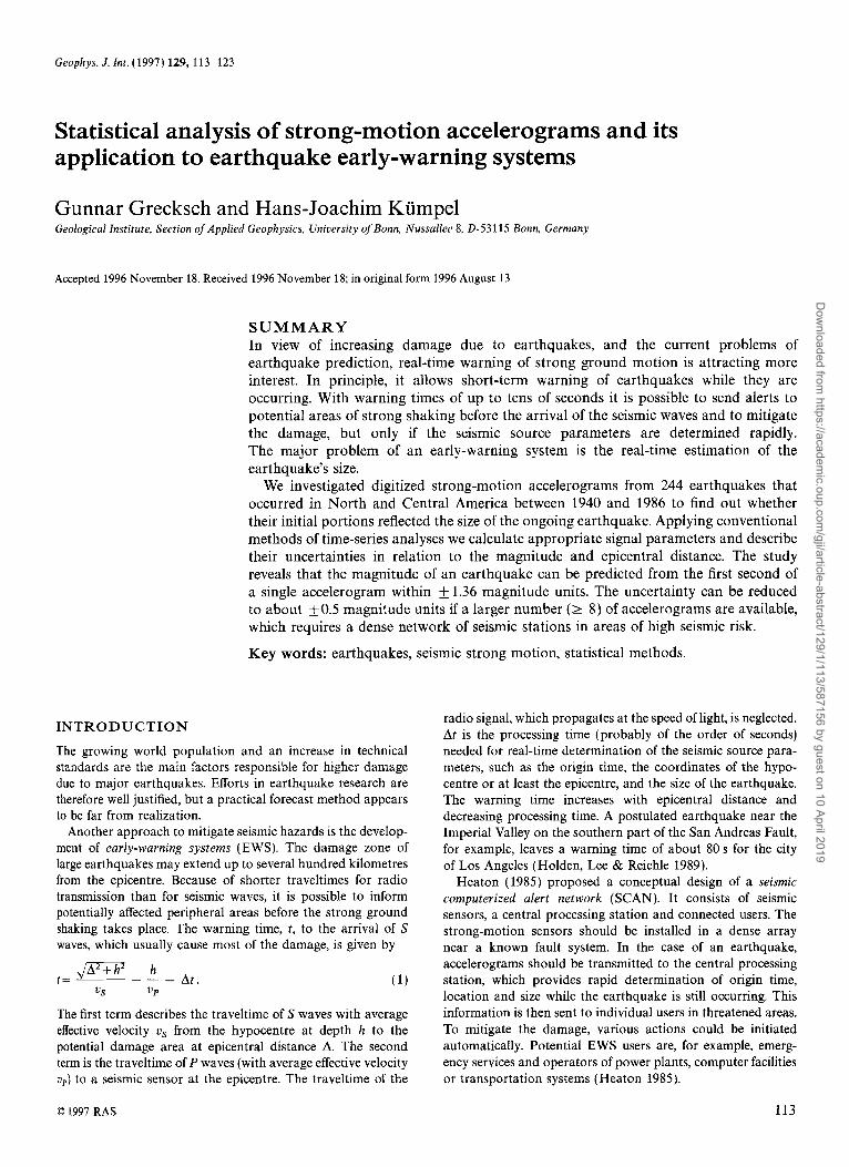
Table 1 summarizes the results of the regression analysis. Apparently, all regression models explain the variations in M L and Mw better than those in M,. Regressions based on the parameters of the resultant acceleration are mostly of lower significance. The introduction oft and l/f does not significantly increase the degree of correlation over that of eq. (4). An

0 1997 RAS, GJI 129, 113-123

Dow




Table 1. Results of the regression analysis.

Vertical acceleration:

M Dependent r b0 bl hz b3 rsd variable

0.66 4.24 0.36 0.61 4.66 0.32 0.30 5.31 0.19 0.65 4.26 0.36 0.61 4.64 0.32 0.31 5.35 0.20 0.67 4.05 0.38 0.64 4.48 0.33 0.33 5.19 0.19 0.67 4.04 0.38 0.64 4.47 0.33 0.34 5.22 0.19 0.71 4.31 0.44 0.62 4.61 0.36 0.52 5.30 0.28

-

~

~

0.59 0.45

- 1.96 0.57 0.56 0.41 0.57 0.60 0.40

-0.75 -0.30 - 1.1 1

~ 0.818 - 0.695 - 1.090 - 0.816 - 0.696 - 1.102 ~ 0.800 - 0.678 ~ 1.091

0.25 0.800 0.11 0.679

-1.78 1.095 - 0.764

0.688 ~ 0.992

Resultant acceleration:

M' Dependent r h0 bl bz b3 rsd variable

~ ~~~ ~~

0.53 4.20 0.32 - ~ 0.891 0.56 4.58 0.29 ~ - 0.735

~ 1.059 ML 0.54 4.16 0.32 2.90 ~ 0.890

bo+b , M * + b 2 t MW 0.56 4.55 0.28 1.50 - 0.736 M s 0.40 4.98 0.25 -5.73 ~ 1.059 ML 0.53 4.13 0.32 0.68 - 0.891

bo+b, M * + b z l/f MW 0.56 4.47 0.28 1.07 ~ 0.735 M s 0.41 4.61 0.23 3.26 - 1.058

0.54 4.12 0.31 0.59 2.77 0.891 ML bo+h, M*+bZ lif +b, t Mw 0.56 4.45 0.28 1.03 1.32 0.736

MS ML 0.60 3.78 0.43 -0.78 ~ 0.843

bo+bl M * + b , log& M w 0.57 4.41 0.32 -0.29 ~ 0.730 MS 0.56 4.47 0.33 -1.14 - 0.957

ML bo+bl M * MW

MS 0.39 4.93 0.24 ~

0.42 4.63 0.25 3.59 -6.48 1.057

example of the situation for the basic regression model (eq. 4) with dependent variable M , is displayed in Fig. 8.

When assuming the presence of a linear relationship in the regression models, the evaluated variables should approxi- mately follow a normal distribution, which has been verified in several cases. Furthermore, the residuals, i.e. the vertical distances of individual data points to the regression line ( M ' - M i , i=L, W or S ) should follow a normal distribution, so that about 68 per cent of the residuals fall within a range of f 1 rsd and about 95 per cent within f 2 rsd of their mean value. Accordingly, rsd describes the fluctuation of the actual magnitudes around the regression line, or is a measure of the inaccuracy of the desired prediction value M'. Considering the far-reaching consequences and the demand for high reliability of an EWS, it appears appropriate to provide predictions with 95 per cent probability.

The smallest rsds are obtained for the regression models of eqs (6) and (7) for the vertical accelerations with M , as the dependent variable. M,, of course, was privileged because this magnitude type was used in establishing eq. ( 2 ) . The correlation coefficients are 0.64, i.e. 41 per cent of the variation

9

0 0

0 0 0 0

0

) O a 0 O

o o B o 0 O 0

0 0

0 0

o o 0

* t -4 -2 0 2 4 6 0 10

M'

Figure 8. Linear regression with independent variable M* and dependent variable M,. The correlation coefficient is r=0.61; the squared correlation yields that the regression explains 37 per cent of the variation. The residual standard deviation is 0.695 magnitude units.

0 1997 RAS, GJI 129, 113-123

Dow




8

5

I 1 1 1 c

San Fernando (Apr. 1971) A- ll --r T ,--r 1-7 -77- 0 20 40 60 80 100 120 140 160 180 200


8

5

1

Coalinga (May 1983)

0 10 20 30 40 50 60 70 Epicentral distance [km]

Morgan Hill (Apr. 1984) Imperial Valley (012. 1979) -7-

20 40 60 80 0 20 40 60 80 100

Epicentral distance [km] Epicentral distance [km] 0

8

7

5

4

3

c I c

i Lytle Creek (Sep. 1970)

v-7- T

Coalinga aftershock (May 1983)

4 t-------r- ?+ 0 20 40 60 80 100 120 0 4 8 12 16

Epicentral distance [km] Epicentral distance [km]

0 1997 RAS, GJI 129, 113-123

Dow




1 1 Hawaii (Nov. 1983)

20 40 60 80 100

T Y -I - 1 7 l r [ 1


L

t

i t L

Alaska (Sep. 1983) 7.- T- -,T 1-r -

70 90 110 130 150 Epicentral distance [krn]

0 5 10 15 20 25 30 35 Epicentral distance [km]

7 1 -1

i 5 1

Alaska (Dec. 1985)


L ' I t

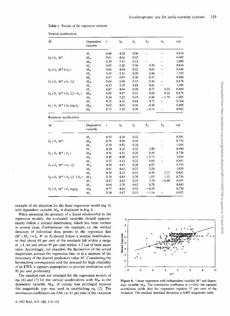
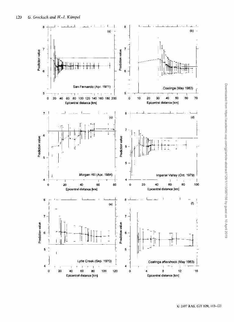
Figure 9. Average magnitude prediction value with Gaussian error versus epicentral distance of accelerograms for single earthquakes. The actual magnitudes are marked by straight lines. (a) San Fernando, April 1971, M,=6.6, number of available accelerograms= 105. (b) Coalinga, May 1983, 6.2, 47. (c) Morgan Hill, April 1984, 6.2, 33. (d) Imperial Valley, October 1979, 6.5, 30. (e) Lytle Creek, September 1970, 5.3, 19. ( f ) Coalinga aftershock, May 1983, 5.2, 18. (g) Hawaii, November 1983, 6.6, 15. (h) Coyote Lake, August 1979, 5.7, 9. (i) Alaska, September 1983, 6.2, 8. (j) Alaska, December 1985, 5.6, 8. The Gaussian error decreases with increasing number of strong-motion records.

of Mw is explained. Since eq. (6) describes the simpler model, and r and rsd are only insignificantly different, it appears to be more suitable than the regression model of eq. (7). This is, however, a preliminary conclusion and requires further investi- gations. Thus, with a 95 per cent statistical probability, the error of a single prediction value M' is at most 1.36 magnitude units. The result of the regression analysis can be summarized as follows.

To some extent it is possible to determine the moment magnitude M , from the first second of the vertical component of a strong-motion accelerogram using the relation

4.48+0.33M*+0.56 - +136, f 'I - '

(9)

with M * as in eq. (3) and jbeing the predominant frequency in the Fourier spectrum.

The uncertainty of 1.36 covers a seismic energy range of four orders of magnitude. Clearly, various inhomogeneities add considerably to the scatter in the data. If we restrict the analysis to individual earthquakes, and magnitude assessments from different accelerograms are stacked, a higher prediction reliability can be expected. In Table 2 an average prediction value as given by the arithmetic mean of the M' values derived from single accelerograms is compared with the actual moment magnitude for 20 different earthquakes. The study was carried out for two maximum epicentral distances, 200 km and 50 km. The associated Gaussian error is

where n is the number of accelerograms and AMri = 1.36. In fact, most of the actual magnitudes M , lie within the reduced

0 1997 RAS, GJI 129, 113-123

Dow



122 G. Grecksch and H.-J. Kumpel

Table 2. Comparison of the actual moment magnitude M , and the average prediction value a’ for maximum epicentral distances up to 200 and 50 km, respectively.

Earthquake Date Number of M , M‘ Gaussian error accelerograms 200 50 200 50 200 50

San Fernando Coalinga Morgan Hill Imperial Valley Lytle Creek Coalinga aftershock Hawaii Coyote Lake Alaska Alaska Borrego Mountain Alaska Parkfield Anza San Francisco Alaska Alaska Alaska Kern County Central California

Apr 71 May 83 Apr 84 Oct 79 Sep 70 May 83 Nov 83 Aug 79 Sep 83 Dez 85 Apr 68 Jul 83 Jun 66 Feb 80 Mar 57 May 82 Oct 85 Jan 75 Jul 52 Apr 80

105 70 6.6 6.25 6.26 0.13 0.16 47 32 6.2 6.12 6.15 0.20 0.24 33 19 6.2 6.25 6.15 0.24 0.31 30 24 6.5 6.09 6.08 0.25 0.28 19 8 5.3 5.82 5.97 0.31 0.48 18 18 5.2 5.57 5.57 0.32 0.32 15 9 6.6 6.22 6.14 0.35 0.45 9 9 5.7 6.09 6.09 0.45 0.45

8 8 5.6 5.80 5.80 0.48 0.48 7 1 6.6 6.41 6.03 0.51 1.36 7 1 6.4 6.39 6.16 0.51 1.36 6 3 6.1 5.87 5.88 0.56 0.79 5 5 5.5 5.59 5.59 0.61 0.61 5 5 5.3 5.48 5.48 0.61 0.61 5 5 4.3 4.98 4.98 0.61 0.61 5 2 6.5 6.18 5.51 0.61 0.96 4 1 6.0 6.26 6.07 0.68 1.36 4 1 7.4 6.51 6.68 0.68 1.36 3 3 4.9 5.49 5.49 0.79 0.79

8 - 6.2 6.41 - 0.48 -

uncertainty interval. Fig. 9 displays the situation for the 10 earthquakes with eight or more accelerograms and maximum epicentral distance 200 km (see also Table 2). The average prediction values and their Gaussian errors are shown as a function of the number of accelerograms arranged with increasing epicentral distance up to the most distant strong-motion record.

The magnitudes of seven earthquakes are rather well approximated by the average prediction value. On the other hand, the actual magnitudes of the San Fernando, the Imperial Valley and the Lytle Creek earthquakes were not found to fall within the uncertainty interval, when 105, 30 and 19 accelerograms were analysed, respectively. This possibly indicates a deficit in applying Gaussian statistics to such data. Since the warning time reduces with increasing epicentral distance (eq. l) , there is a trade-off between prediction quality and warning time. The more strong-motion sensors are operating in the epicentral area, the more reliable the magnitude prediction could be made. Our analysis shows that eight sensors could reduce the 95 per cent uncertainty to about 0.5 magnitude units. Accordingly, despite a considerable remaining error the average prediction value could be a useful real-time estimate of the moment magnitude of an ongoing earthquake.

CONCLUSION

The major problem of an early-warning system (EWS), which should provide short-term warnings to potential areas of strong shaking before the arrival of seismic waves, is the real-time estimation of the earthquake’s size. To find out whether the first second of digitized strong-motion accelerograms contains reliable information on the magnitude of the ongoing earthquake, we investigated data from 244 earthquakes in North

and Central America that were recorded between 1940 and 1986. Applying standard methods of time-series analysis, we calculated the peak acceleration, the rise time of the first complete peak, the predominant frequency and the related Fourier amplitude to use these parameters in linear regression models that are simple extensions of Joyner & Boore’s (1981) empirical relation (eq. 2) between the actual magnitude, acceleration amplitude and epicentral distance of the strong- motion sensors.

In fact, the magnitude of all earthquakes can to some extent be predicted from the initial part of the strong-motion signals. The 95 per cent uncertainty is, however, f 1.36 if the prediction is based on a single accelerogram. Converting this into units of seismic energy yields an uncertainty of four orders of magnitude, which seems to be inappropriate for an EWS. The uncertainty can be reduced significantly by computing an average prediction value from a larger number of accelerograms, which requires a dense network of seismic stations in the epicentral area of the ongoing earthquake. Eight strong- motion sensors, for example, preferably with a good azimuthal distribution, would generally be sufficient to reduce the 95 per cent uncertainty to about k0.5 magnitude units, which corresponds to a factor 30 in energy range. Similarly, the network could be used for the fast location of the earthquake epicentre by processing differences in arrival times.

Despite a considerable error, the average prediction value appears to be a useful real-time estimate of the magnitude. The prediction quality can probably be improved when regional aspects like site effects or the depth of the rupture zone are taken into account; they were not considered here. Further improvements may result from progress in instrumental design, e.g. installation of digital strong-motion sensor networks as recommended by the US National Research Council (1991).

0 1997 RAS, GJI 129, 113-123

Dow




ACKNOWLEDGMENTS

We thank the USGS for making the collection of digitized strong-motion accelerograms available on CD-ROM. Helpful comments from M. Nicolas and an anonymous reviewer on the original version of the manuscript are appreciated.

NOTE ADDED I N PROOF

After this article had passed the review, we became aware of a paper by Hardt & Scherbaum (1996). The authors describe an approach in part similar to ours, and present detailed time- history estimates of magnitude probability distributions for three Loma Prieta aftershocks (1989, M : 2.4, 3.8, 4.5) and for the M 6.7 Northridge earthquake of January 1994, California, based on accelerograms from several stations of the individual events.

REFERENCES

Bakun, W.H., Fischer, F.G., Jensen, E.G. & VanSchaack, J., 1994. Early warning system for aftershocks, Bull. seism. Soc. Am., 84,

Converse, A.M., 1992. BAP: Basic strong-motion accelerogram processing software, Version 1.0, US Geological Survey, Open File Report 92-296 A & 92-296B.

Hardt, M. & Scherbaum, F., 1996. Early warning system design: performance test for multi-method magnitude determination,

359-365.

Cahiers du Centre EuropCen de GCodynamique et de Seismologie, eds Garcia-Fernandez, M. & Zonno, G., 12, 225-236.

Heaton, T.H., 1985. A model for a seismic computerized alert network, Science, 228, 987-990.

Holden, R., Lee, R. & Reichle, M., 1989. Technical and economic feasibility of an earthquake warning system in California, Calif. Dept. of Conservation Special Publ., 101.

Joyner, W.B. & Boore, D.M., 1981. Peak horizontal acceleration and velocity from strong-motion records including records from the 1979 Imperial Valley, California, Earthquake, Bull. seism. Soc. Am., 71,

Kanamori, H., Hauksson, E. & Heaton, T., 1991. TERRAscope and CUBE Project at Caltech, EOS, Trans. Am. geophys. Un., 72, No. 50, 564.

Nakamura, Y., 1989. Earthquake alarm system for Japan Railways, Japanese Railway Engineering, 109, 1-7.

Nakamura, Y. , 1995. Development of natural disaster prevention systems, Quarterly Rept Railway Technical Research Institute

Seekins, L.C., Brady, A.G., Carpenter, C. & Brown, N., 1992. Digitized strong-motion accelerograms of North and Central American earthquakes 1933-1986, US Geological Survey Digital Data Series DDS-7.

Toksoz, M.N., Dainty, A.M. & Bullitt, J.T., 1990. A prototype earthquake warning system for strike-slip earthquakes, PAGEOPH, 133,

Trifunac, M.D., Udwadia, F.E. & Brady, A.G., 1973. Analysis of errors in digitized strong-motion accelerograms, Bull. seism. Soc. Am.,

US National Research Council, 1991. Real-time earthquake

2011-2038.

( R T R I ) , 36, NO. 1, 8-12.

475-487.

63, 157-187.

monitoring, National Academy Press, Washington, DC.

0 1997 RAS, GJI 129, 113-123

Dow



Documents

Statistical analysis of strong-motion accelerograms and its