Embed Size (px)
Citation preview
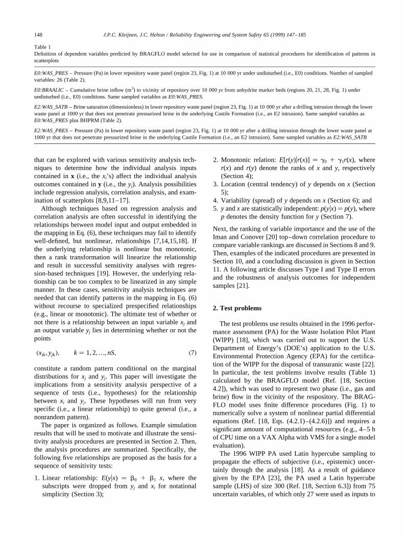
Statistical analyses of scatterplots to identify important factors in large-scale simulations, 1: Review and comparison of techniques
J.P.C. Kleijnena, J.C. Heltonb,*aDepartment of Information Systems, Tilburg University, 5000 LE Tilburg, The Netherlands
bDepartment of Mathematics, Arizona State University, Tempe, AZ 85287-1804, USA
Received 10 April 1998; accepted 25 September 1998
Abstract
Procedures for identifying patterns in scatterplots generated in Monte Carlo sensitivity analyses are described and illustrated. Theseprocedures attempt to detect increasingly complex patterns in scatterplots and involve the identification of (i) linear relationships withcorrelation coefficients, (ii) monotonic relationships with rank correlation coefficients, (iii) trends in central tendency as defined by means,medians and the Kruskal–Wallis statistic, (iv) trends in variability as defined by variances and interquartile ranges, and (v) deviations fromrandomness as defined by the chi-square statistic. A sequence of example analyses with a large model for two-phase fluid flow illustrates howthe individual procedures can differ in the variables that they identify as having effects on particular model outcomes. The example analysesindicate that the use of a sequence of procedures is a good analysis strategy and provides some assurance that an important effect is notoverlooked.q 1999 Elsevier Science Ltd. All rights reserved.
Keywords:Chi-square; Correlation coefficient; Epistemic uncertainty; Interquartile range; Kruskal–Wallis; Latin hypercube sampling; Mean; Median; MonteCarlo; Partial correlation coefficient; Rank transform; Scatterplot; Sensitivity analysis; Standarized regression coefficient; Subjective uncertainty; Top–downcorrelation; Variance
1. Introduction
Sensitivity analysis is now widely recognized as an essen-tial component of studies based on mathematical modeling(e.g., Refs. [1–6]). Here, sensitivity analysis refers to thedetermination of the effects of uncertain model inputs onmodel predictions. A number of methods have beenproposed for sensitivity analysis, including differentialanalysis, response surface methodologies, Monte Carlotechniques, and the Fourier amplitude sensitivity test [7–9].
Monte Carlo techniques probably constitute the mostwidely used approach to sensitivity analysis owing to theirflexibility, ease of implementation, and conceptual simpli-city. When viewed abstractly, a Monte Carlo sensitivitystudy involves a vector
x � �x1; x2;…; xnI� �1�of uncertain model inputs, where eachxi is an uncertaininput andnI is the number of such inputs, and a vector
y � f �x� � �y1; y2;…; ynO� �2�
of model predictions, wheref is a function used to representthe model under consideration, eachyj is an outcome ofevaluating the model with the inputx, andnO is the numberof such outcomes. Distributions
Di ; i � 1;2;…; nI; �3�are used to characterize the uncertainty in each inputxi,where Di is the distribution assigned toxi. Correlationsand other relationships between thexi are also possible.
A sampling procedure such as simple random sampling orLatin hypercube sampling [10] is used to generate a sample
xk � �x1k; x2k;…; xnI;k�; k � 1; 2;…;nS; �4�from the population ofx’s with the distributions in Eq. (3),wherenSis the size of the sample. Evaluation of the modelunder consideration with the sample elementsxk in Eq. (4)then creates a sequence of results of the form
yk � f �xk� � �y1k; y2k;…; ynO;k�; k � 1;2;…;nS; �5�where eachyjk is a particular outcome of evaluating themodel withxk. The pairs
�xk; yk�; k � 1;2;…; nS; �6�constitute a mapping from model inputxk to model outputyk
Reliability Engineering and System Safety 65 (1999) 147–185
0951-8320/99/$ - see front matterq 1999 Elsevier Science Ltd. All rights reserved.PII: S0951-8320(98)00091-X
* Corresponding author. Tel.:1 1-505-284-4808; Fax:1 1-505-844-2348.
E-mail address:[email protected] (J.C. Helton)
that can be explored with various sensitivity analysis tech-niques to determine how the individual analysis inputscontained inx (i.e., thexi’s) affect the individual analysisoutcomes contained iny (i.e., theyj). Analysis possibilitiesinclude regression analysis, correlation analysis, and exam-ination of scatterplots [8,9,11–17].
Although techniques based on regression analysis andcorrelation analysis are often successful in identifying therelationships between model input and output embedded inthe mapping in Eq. (6), these techniques may fail to identifywell-defined, but nonlinear, relationships [7,14,15,18]. Ifthe underlying relationship is nonlinear but monotonic,then a rank transformation will linearize the relationshipand result in successful sensitivity analyses with regres-sion-based techniques [19]. However, the underlying rela-tionship can be too complex to be linearized in any simplemanner. In these cases, sensitivity analysis techniques areneeded that can identify patterns in the mapping in Eq. (6)without recourse to specialized prespecified relationships(e.g., linear or monotonic). The ultimate test of whether ornot there is a relationship between an input variablexj andan output variableyj lies in determining whether or not thepoints
�xik; yjk�; k � 1;2;…; nS; �7�
constitute a random pattern conditional on the marginaldistributions forxj and yj. This paper will investigate theimplications from a sensitivity analysis perspective of asequence of tests (i.e., hypotheses) for the relationshipbetweenxi and yj. These hypotheses will run from veryspecific (i.e., a linear relationship) to quite general (i.e., anonrandom pattern).
The paper is organized as follows. Example simulationresults that will be used to motivate and illustrate the sensi-tivity analysis procedures are presented in Section 2. Then,the analysis procedures are summarized. Specifically, thefollowing five relationships are proposed as the basis for asequence of sensitivity tests:
1. Linear relationship:E(yux) � b0 1 b1 x, where thesubscripts were dropped fromyj and xi for notationalsimplicity (Section 3);
2. Monotonic relation:E[r(y)ur(x)] � g0 1 g1r(x), wherer(x) and r(y) denote the ranks ofx and y, respectively(Section 4);
3. Location (central tendency) ofy depends onx (Section5);
4. Variability (spread) ofy depends onx (Section 6); and5. y andx are statistically independent:p(yux)� p(y), where
p denotes the density function fory (Section 7).
Next, the ranking of variable importance and the use of theIman and Conover [20] top–down correlation procedure tocompare variable rankings are discussed in Sections 8 and 9.Then, examples of the indicated procedures are presented inSection 10, and a concluding discussion is given in Section11. A following article discusses Type I and Type II errorsand the robustness of analysis outcomes for independentsamples [21].
2. Test problems
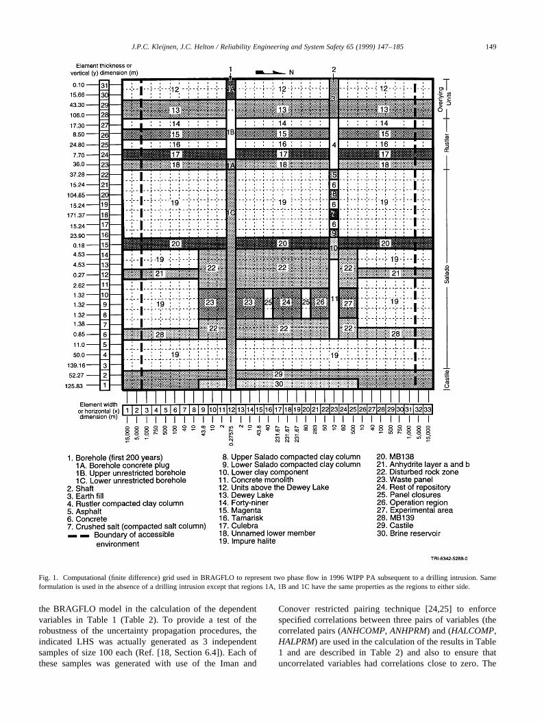
The test problems use results obtained in the 1996 perfor-mance assessment (PA) for the Waste Isolation Pilot Plant(WIPP) [18], which was carried out to support the U.S.Department of Energy’s (DOE’s) application to the U.S.Environmental Protection Agency (EPA) for the certifica-tion of the WIPP for the disposal of transuranic waste [22].In particular, the test problems involve results (Table 1)calculated by the BRAGFLO model (Ref. [18, Section4.2]), which was used to represent two phase (i.e., gas andbrine) flow in the vicinity of the respository. The BRAG-FLO model uses finite difference procedures (Fig. 1) tonumerically solve a system of nonlinear partial differentialequations (Ref. [18, Eqs. (4.2.1)–(4.2.6)]) and requires asignificant amount of computational resources (e.g., 4–5 hof CPU time on a VAX Alpha with VMS for a single modelevaluation).
The 1996 WIPP PA used Latin hypercube sampling topropagate the effects of subjective (i.e., epistemic) uncer-tainly through the analysis [18]. As a result of guidancegiven by the EPA [23], the PA used a Latin hypercubesample (LHS) of size 300 (Ref. [18, Section 6.3]) from 75uncertain variables, of which only 27 were used as inputs to
J.P.C. Kleijnen, J.C. Helton / Reliability Engineering and System Safety 65 (1999) 147–185148
Table 1Definition of dependent variables predicted by BRAGFLO model selected for use in comparison of statistical procedures for identification of patternsinscatterplots
E0:WAS_PRES– Pressure (Pa) in lower repository waste panel (region 23, Fig. 1) at 10 000 yr under undisturbed (i.e., E0) conditions. Number of sampledvariables: 26 (Table 2).
E0:BRAALIC– Cumulative brine inflow (m3) to vicinity of repository over 10 000 yr from anhydrite marker beds (regions 20, 21, 28, Fig. 1) underundisturbed (i.e., E0) conditions. Same sampled variables asE0:WAS_PRES.
E2:WAS_SATB– Brine saturation (dimensionless) in lower repository waste panel (region 23, Fig. 1) at 10 000 yr after a drilling intrusion through the lowerwaste panel at 1000 yr that does not penetrate pressurized brine in the underlying Castile Formation (i.e., an E2 intrusion). Same sampled variables asE0:WAS_PRESplus BHPRM (Table 2).
E2:WAS_PRES– Pressure (Pa) in lower repository waste panel (region 23, Fig. 1) at 10 000 yr after a drilling intrusion through the lower waste panel at1000 yr that does not penetrate pressurized brine in the underlying Castile Formation (i.e., an E2 intrusion). Same sampled variables asE2:WAS_SATB
the BRAGFLO model in the calculation of the dependentvariables in Table 1 (Table 2). To provide a test of therobustness of the uncertainty propagation procedures, theindicated LHS was actually generated as 3 independentsamples of size 100 each (Ref. [18, Section 6.4]). Each ofthese samples was generated with use of the Iman and
Conover restricted pairing technique [24,25] to enforcespecified correlations between three pairs of variables (thecorrelated pairs (ANHCOMP, ANHPRM) and (HALCOMP,HALPRM) are used in the calculation of the results in Table1 and are described in Table 2) and also to ensure thatuncorrelated variables had correlations close to zero. The
J.P.C. Kleijnen, J.C. Helton / Reliability Engineering and System Safety 65 (1999) 147–185 149
Fig. 1. Computational (finite difference) grid used in BRAGFLO to represent two phase flow in 1996 WIPP PA subsequent to a drilling intrusion. Sameformulation is used in the absence of a drilling intrusion except that regions 1A, 1B and 1C have the same properties as the regions to either side.
J.P.C. Kleijnen, J.C. Helton / Reliability Engineering and System Safety 65 (1999) 147–185150
Table 2Uncertain variables used as input to BRAGFLO in the calculation of the dependent variables in Table 1 (see, Ref. [18, Table 5.2.1] and Ref. [22, App. PAR], foradditional information and a discussion of all 75 variables included in the LHS)
ANHBCEXP– Brooks–Corey pore distribution parameter for anhydrite (dimensionless). Distribution: Student’s with 5 degrees of freedom. Range: 0.491–0.842. Mean, median: 0.644.
ANHBCVGP– Pointer variable for selection of relative permeability model for use in anhydrite. Distribution: Discrete with 60% 0, 40% 1. Value of 0 impliesBrooks–Corey model; value of 1 implies van Genuchten–Parker model.
ANHCOMP– Bulk compressibility of anhydrite (Pa21). Distribution: Student’s with 3 degrees of freedom. Range: 1.09× 10211 to 2.75× 10210 Pa21. Mean,median: 8.26× 10211 Pa21. Correlation: 2 0.99 rank correlation [23] withANHPRM. Variable 21 in LHS.
ANHPRM– Logarithm of anhydrite permeability (m2). Distribution: Student’s with 5 degrees of freedom. Range:2 21.0 to 2 17.1 (i.e., permeability rangeis 1 × 10221 to 1 × 10217.1 m2). Mean, median:2 18.9. Correlation:2 0.99 rank correlation withANHCOMP.
ANRBRSAT– Residual brine saturation in anhydrite (dimensionless). Distribution: Student’s with 5 degrees of freedom. Range: 7.85× 10²³ to 1.74× 10²¹.Mean, median: 8.36× 10²².
ANRGSSAT– Residual gas saturation in anhydrite (dimensionless). Distribution: Student’s with 5 degrees of freedom. Range: 1.39× 10²² to 1.79× 10²¹.Mean, median: 7.71× 10²².
BHPRM– Logarithm of borehole permeability (m2). Distribution: Uniform. Range:2 14 to 2 11 (i.e., permeability range is 1× 10214 to 1 × 10211 m2).Mean, median:2 12.5.
HALCOMP– Bulk compressibility of halite (Pa21). Distribution: Uniform. Range: 2.94× 10212 to 1.92× 10210 Pa21. Mean, median: 9.75× 10211 Pa21,9.75× 10211 Pa21. Correlation: 2 0.99 rank correlation withHALPRM.
HALPOR– Halite porosity (dimensionless). Distribution: Piecewise uniform. Range: 1.0× 10²³ to 3 × 10²². Mean, median: 1.28× 10²², 1.00× 10²².
HALPRM– Logarithm of halite permeability (m2). Distribution: Uniform. Range:2 24 to 2 21 (i.e., permeability range is 1× 10224 to 1 × 10221 m2).Mean, median:2 22.5, 2 22.5. Correlation:2 0.99 rank correlation withHALCOMP.
SALPRES– Initial brine pressure, without the repository being present, at a reference point located in the center of the combined shafts at the elevation of themidpoint of MB 139 (Pa). Distribution: Uniform. Range: 1.104× 10⁷ to 1.389× 10⁷ Pa. Mean, median: 1.247× 10⁷ Pa, 1.247× 10⁷ Pa.
SHBCEXP– Brooks–Corey pore distribution parameter for shaft (dimensionless). Distribution: Piecewise uniform. Range: 0.11–8.10. Mean, median: 2.52,0.94.
SHPRMASP– Logarithm of permeability (m2) of asphalt component of shaft seal (m2). Distribution: Triangular. Range:2 21 to 2 18 (i.e., permeabilityrange is 1× 10221 to 1 × 10218 m2). Mean, mode:2 19.7, 2 20.0.
SHPRMCLY– Logarithm of permeability (m2) for clay components of shaft. Distribution: Triangular. Range:2 21 to 2 17.3 (i.e., permeability range is 1×10221 to 1 × 10217.3 m2). Mean, mode:2 18.9, 2 18.3.
SHPRMCON– Same asSHPRMASPbut for concrete component of shaft seal for 0–400 yr. Distribution: Triangular. Range:2 17.0 to 2 14.0 (i.e.,permeability range is 1× 10217 to 1 × 10214 m2). Mean, mode:2 15.3, 2 15.0.
SHPRMDRZ– Logarithm of permeability (m2) of DRZ surrounding shaft. Distribution: Triangular. Range:2 17.0 to 2 14.0 (i.e., permeability range is 1×10217 to 1 × 10214 m2). Mean, mode:2 15.3, 2 15.0.
SHPRMHAL– Pointer variable (dimensionless) used to select permeability in crushed salt component of shaft seal at different times. Distribution: Uniform.Range: 0–1. Mean, mode: 0.5, 0.5. A distribution of permeability (m2) in the crushed salt component of the shaft seal is defined for each of the following timeintervals: [0,10 yr], [10,25 yr], [25,50 yr], [50,100 yr], [100,200 yr], [200,10 000 yr].SHPRMHALis used to select a permeability value from the cumulativedistribution function for permeability for each of the preceding time intervals with result that a rank correlation of 1 exists between the permeabilities used forthe individual time intervals.
SHRBRSAT– Residual brine saturation in shaft (dimensionless). Distribution: Uniform. Range: 0–0.4. Mean, median: 0.2, 0.2.
SHRGSSAT– Residual gas saturation in shaft (dimensionless). Distribution: Uniform. Range: 0–0.4. Mean, median: 0.2, 0.2.
WASTWICK– Increase in brine saturation of waste owing to capillary forces (dimensionless). Distribution: Uniform. Range: 0–1. Mean, median: 0.5, 0.5.
WFBETCEL– Scale factor used in definition of stoichiometric coefficient for microbial gas generation (dimensionless). Distribution: Uniform. Range: 0–1.Mean, median: 0.5, 0.5.
WGRCOR– Corrosion rate for steel under inundated conditions in the absence of CO2 (m/s). Distribution: Uniform. Range: 0–1.58× 10214 m/s. Mean,median: 7.94× 10215 m/s, 7.94× 10215 m/s.
WGRMICH– Microbial degradation rate for cellulose under humid conditions (mol/kg s). Distribution: Uniform. Range: 0 to 1.27× 1029 mol/kg s. Mean,median: 6.34× 10210 mol/kg s, 6.34× 10210 mol/kg s.
WGRMICI– Microbial degradation rate for cellulose under inundated conditions (mol/kg s). Distribution: Uniform. Range: 3.17× 10210 to 9.51× 1029 mol/kg s. Mean, median: 4.92× 1029 mol/kg s, 4.92× 1029 mol/kg s.
WMICDFLG– Pointer variable for microbial degradation of cellulose. Distribution: Discrete, with 50% 0, 25% 1, 25% 2. WMICDFLG� 0, 1, 2 implies nomicrobial degradation of cellulose, microbial degradation of only cellulose, microbial degradation of cellulose, plastic and rubber.
WRBRNSAT– Residual brine saturation in waste (dimensionless). Distribution: Uniform. Range: 0–0.552. Mean, median: 0.276, 0.276.
WRGSSAT– Residual gas saturation in waste (dimensionless). Distribution: Uniform. Range: 0–0.15. Mean, median: 0.075, 0.075.
outcome of this sampling was 3 LHSs of size 100 each:
R1 : x1k � �x1k1; x1k2;…; x1k75�; k � 1; 2;…;100; �8�
R2 : x2k � �x2k1; x2k2;…; x2k75�; k � 1; 2;…;100; �9�
R3 : x3k � �x3k1; x3k2;…; x3k75�; k � 1; 2;…;100; �10�wherex � �x1; x2;…; x75� corresponds to the 75 uncertainvariables indicated in Table 2 andR1, R2 andR3 designatethe three replicated (i.e., independently generated) LHSs.
Once the LHSs in Eqs. (8)–(10) were generated, BRAG-FLO calculations were performed for a variety of cases(Ref. [18, Table 6.9.1]). The two cases considered hereare (i) undisturbed (i.e., E0) conditions, and (ii) a drillingintrusion through the lower waste panel at 1000 yr that doesnot penetrate pressurized brine in the underlying CastileFormation (i.e., E2 conditions or, in the more detailed
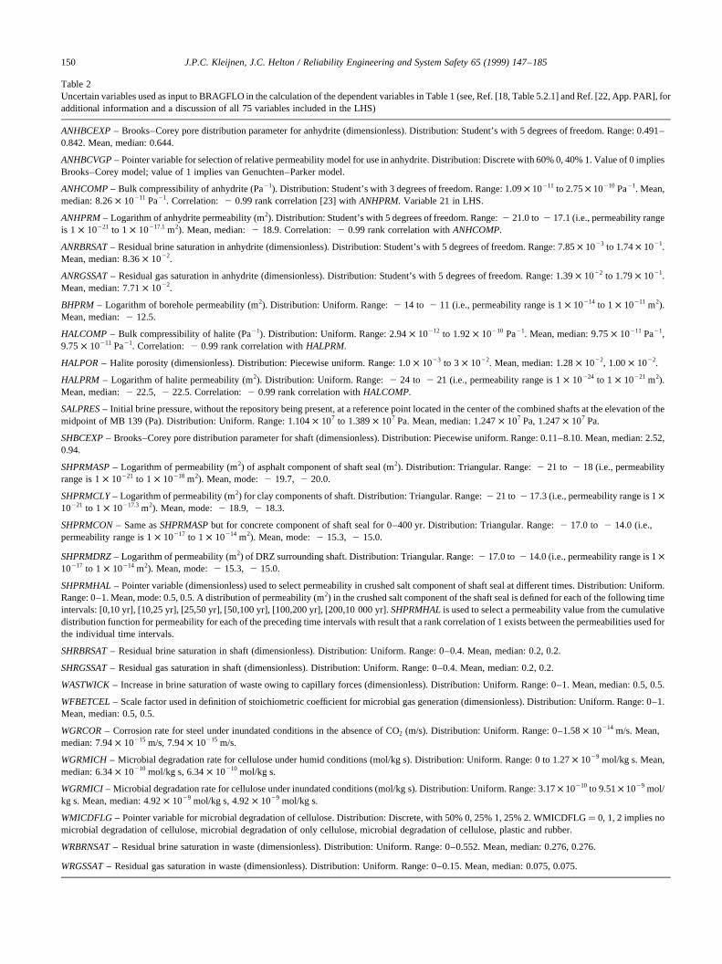
descriptions given in Ref. [18], E2 conditions with theintrusion occuring at 1000 yr). Results calculated byBRAGFLO are time-dependent. The time-dependent beha-vior of the results is shown in Fig. 2 for replicateR1. Forsimplicity, the technique comparisons will use the values ofthe variables at the end points of the individual curves inFig. 2 (i.e., at 10 000 yr). However, nothing preventsanalyses at other times and, in general, sensitivity analysesof time-dependent variables should also be time-dependent(Ref. [18, Chapters 7 and 8]).
For perspective and motivation, regression-based resultsfor the variables in Table 1 (obtained in Ref. [18] with theSTEP program [26]) are presented in Table 3 for both rawand rank-transformed data. In Table 3, a variable wasrequired to be significant at ana-value of 0.02 to enter aregression model and to remain significant at ana-value of0.05 to be retained in a regression model, although there
J.P.C. Kleijnen, J.C. Helton / Reliability Engineering and System Safety 65 (1999) 147–185 151
Fig. 2. Dependent variables predicted by BRAGFLO model: (a) pressure in lower waste panel under undisturbed conditions (E0:WAS_PRES), (b) cumulativebrine inflow from anhydrite marker beds under undisturbed conditions (E0: BRAALIC), (c) saturation in lower waste panel after an E2 intrusion at 1000 yr (E2:WAS_SATB), and (d) pressure in lower waste panel after an E2 intrusion at 1000 yr (E2: WAS_PRES).
were no cases of a variable entering and then being droppedfrom a regression model. As will be seen, the rank-transfor-mation is often an effective procedure for improving theresolution of regression-based sensitivity analyses.However, as will also be seen, nonmonotonic relationshipscan result in patterns that cannot be effectively analyzedwith rank-transformed data. It is the need to be able toidentify such patterns that forms the motivation for thisstudy.
The analyses in Table 3 for repository pressure underundisturbed conditions (E0:WAS_PRES) with raw andrank-transformed data are reasonably effective, with
1. R2 values of 0.82 and 0.81 for raw and rank-transformeddata,
2. the same variables selected in both analyses, and3. only one minor variation in the order of variable selec-
tion (i.e., the order of selection of the last two variables inthe regression models is reversed).
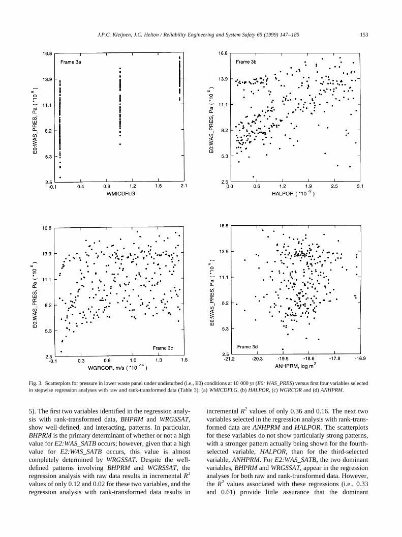
Scatterplots for the first four variables selected in the regres-sion anlayses forE0:WAS_PRESare presented in Fig. 3.The scatterplots for the first two variables selected in theregression analysis,WMICDFLG and HALPOR, displaywell-defined patterns. The pattern for the third variable,WGRCOR, is weaker but still detectable. The fourth vari-able,ANHPRM, changes theR2 values for raw and rank-transformed data by 0.02 and 0.01, respectively, andproduces a scatterplot that displays little discernible pattern.
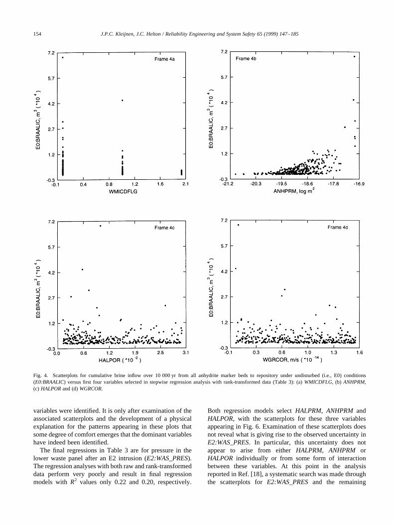
The analyses for cumulative brine inflow from all anhy-drite marker beds to the repository under undisturbed condi-tions (E0:BRAALIC) are interesting in that the regressionwith raw data is not particularly effective (i.e.,R2� 0.50 atfinal step of analysis), whereas the regression with rank-transformed data is reasonably successful in accountingfor the observed uncertainty (i.e.,R2� 0.87). Again, exam-ination of scatterplots shows well-defined patterns for thefirst two variables,WMICDFLGandANHPRM, selected inboth regression analyses (Fig. 4). Scatterplots for the nexttwo variables,HALPOR and WGRCOR, selected in theregression analysis with rank-transformed data are alsogiven in Fig. 4. The negative effects of these variables, asindicated by the signs of their standardized regression coef-ficients, are barely discernible in their scatterplots, withthese small effects being consistent with observed changesin R2 values of 0.05 and 0.02 with the entry ofHALPORandWGRCOR, respectively, into the regression model. In thisexample, the regression analyses with both raw and rank-transformed data have identified the two dominant vari-ables,WMICDFLG and ANHPRM. However, the analysiswith raw data in isolation would not be very credible owingto its low R2 value.
The regression analysis with raw data for brine saturationin the lower waste panel after an E2 intrusion(E2:WAS_SATB) is quite poor, with the final regressionmodel containing 6 variables but having anR2 value ofonly 0.33. The regression analysis with rank-transformed
data does somewhat better and results in a final regressionmodel with 6 variables and anR2 value of 0.61. However, anR2 value of 0.61 is not particularly reassuring with respect towhether or not all the variables giving rise to the observeduncertainty inE2:WAS_SATBwere identified. Additionalinsights can be obtained by examining scatterplots (Fig.
J.P.C. Kleijnen, J.C. Helton / Reliability Engineering and System Safety 65 (1999) 147–185152
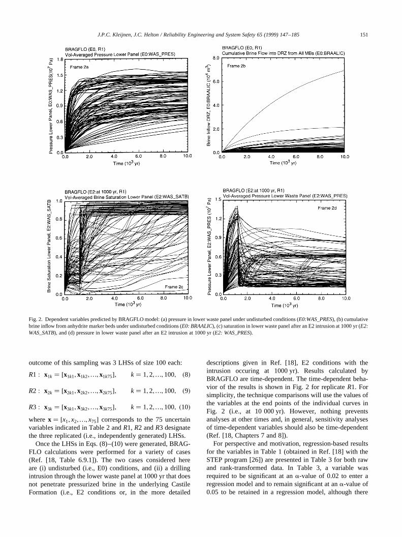
Table 3Stepwise regression analyses with raw and rank-transformed data withpooled results from replicates R1, R2 and R3 (i.e., for a total of 300observations) for output variablesE0:WAS_PRES, E0:BRAALIC,E2:WAS_SATBandE2:WAS_PRESat 10 000 yr
Raw data,E0:WAS_PRES Rank-trasnformed data,E0:WAS_PRES
Stepa Variableb SRCc R2d Variableb SRRCe R2d
1 WMICDFLG 0.72 0.51 WMICDFLG 0.71 0.522 HALPOR 0.47 0.73 HALPOR 0.45 0.733 WGRCOR 0.25 0.79 WGRCOR 0.23 0.794 ANHPRM 0.13 0.81 ANHPRM 0.11 0.805 SHRGSSAT 0.07 0.81 SALPRES 0.07 0.806 SALPRES 0.06 0.82 SHRGSSAT 0.06 0.81
Raw data,E0:BRAALIC Rank-trasnformed data,E0:BRAALIC
Step Variable SRC R2 Variable SRRC R2
1 ANHPRM 0.56 0.32 WMICDFLG 2 0.66 0.432 WMICDFLG 2 0.31 0.42 ANHPRM 0.59 0.753 WGRCOR 2 0.16 0.45 HALPOR 2 0.16 0.804 WASTWICK 2 0.15 0.47 WGRCOR 2 0.15 0.825 ANHBCEXP 2 0.12 0.49 HALPRM 0.14 0.856 HALPOR 2 0.10 0.50 SALPRES 0.12 0.867 WASTWICK 2 0.10 0.87
Raw data,E2:WAS_SATB Rank-transformed data,E2:WAS_SATB
Step Variable SRC R2 Variable SRRC R2
1 BHPRM 0.37 0.12 BHPRM 0.59 0.362 ANHPRM 0.30 0.21 WRGSSAT 2 0.40 0.523 HALPOR 0.21 0.25 ANHPRM 0.23 0.574 WGRCOR 2 0.19 0.29 HALPOR 0.13 0.595 WRGSSAT 2 0.15 0.31 SHPRMHAL 2 0.12 0.606 WMICDFLG 2 0.14 0.33 WGRCOR 2 0.10 0.61
Raw data,E2:WAS_PRES Rank-transformed data,E2:WAS_PRES
Step Variable SRC R2 Variable SRRC R2
1 HALPRM 0.37 0.14 HALPRM 0.36 0.132 ANHPRM 0.24 0.20 ANHPRM 0.24 0.193 HALPOR 0.14 0.22 HALPOR 0.14 0.20
a Steps in stepwise regression analysis.b Variables listed in order of selection in regression analysis with
ANHCOMPand HALCOMP excluded from entry into regression modelbecause of 2 0.99 rank correlation within the pairs (ANHPRM,ANHCOMP) and (HALPRM, HALCOMP).
c Standardized regression coefficients (SRCs) in final regression model.d CumulativeR2value with entry of each variable into regression model.e Standardized rank regression coefficients (SRRCs) in final regression
model.
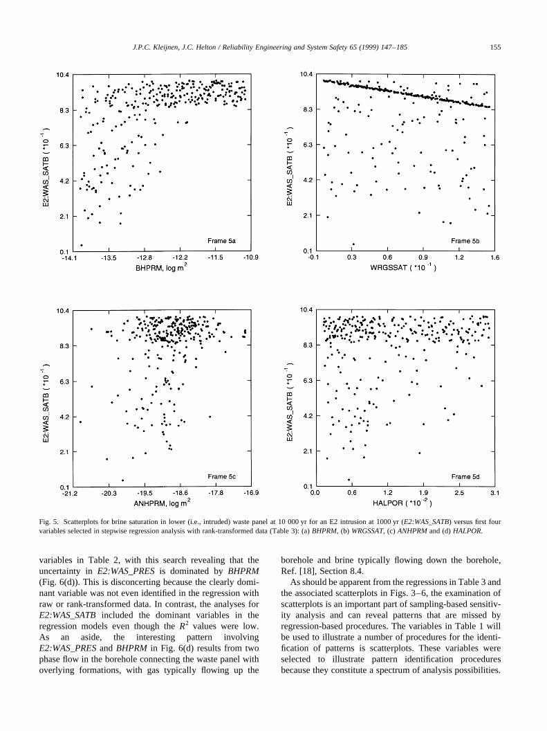
5). The first two variables identified in the regression analy-sis with rank-transformed data,BHPRM and WRGSSAT,show well-defined, and interacting, patterns. In particular,BHPRMis the primary determinant of whether or not a highvalue forE2:WAS_SATBoccurs; however, given that a highvalue for E2:WAS_SATBoccurs, this value is almostcompletely determined byWRGSSAT. Despite the well-defined patterns involvingBHPRM and WGRSSAT, theregression analysis with raw data results in incrementalR2
values of only 0.12 and 0.02 for these two variables, and theregression analysis with rank-transformed data results in
incrementalR2 values of only 0.36 and 0.16. The next twovariables selected in the regression analysis with rank-trans-formed data areANHPRMandHALPOR. The scatterplotsfor these variables do not show particularly strong patterns,with a stronger pattern actually being shown for the fourth-selected variable,HALPOR, than for the third-selectedvariable,ANHPRM. For E2:WAS_SATB, the two dominantvariables,BHPRMandWRGSSAT, appear in the regressionanalyses for both raw and rank-transformed data. However,the R2 values associated with these regressions (i.e., 0.33and 0.61) provide little assurance that the dominant
J.P.C. Kleijnen, J.C. Helton / Reliability Engineering and System Safety 65 (1999) 147–185 153
Fig. 3. Scatterplots for pressure in lower waste panel under undisturbed (i.e., E0) conditions at 10 000 yr (E0: WAS_PRES) versus first four variables selectedin stepwise regression analyses with raw and rank-transformed data (Table 3): (a)WMICDFLG, (b) HALPOR, (c) WGRCORand (d)ANHPRM.
variables were identified. It is only after examination of theassociated scatterplots and the development of a physicalexplanation for the patterns appearing in these plots thatsome degree of comfort emerges that the dominant variableshave indeed been identified.
The final regressions in Table 3 are for pressure in thelower waste panel after an E2 intrusion (E2:WAS_PRES).The regression analyses with both raw and rank-transformeddata perform very poorly and result in final regressionmodels withR2 values only 0.22 and 0.20, respectively.
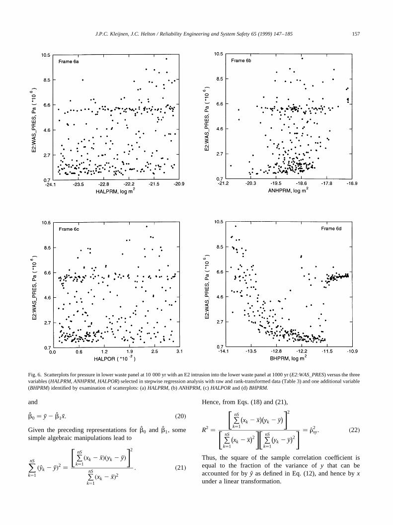
Both regression models selectHALPRM, ANHPRM andHALPOR, with the scatterplots for these three variablesappearing in Fig. 6. Examination of these scatterplots doesnot reveal what is giving rise to the observed uncertainty inE2:WAS_PRES. In particular, this uncertainty does notappear to arise from eitherHALPRM, ANHPRM orHALPOR individually or from some form of interactionbetween these variables. At this point in the analysisreported in Ref. [18], a systematic search was made throughthe scatterplots forE2:WAS_PRESand the remaining
J.P.C. Kleijnen, J.C. Helton / Reliability Engineering and System Safety 65 (1999) 147–185154
Fig. 4. Scatterplots for cumulative brine inflow over 10 000 yr from all anhydrite marker beds to repository under undisturbed (i.e., E0) conditions(E0:BRAALIC) versus first four variables selected in stepwise regression analysis with rank-transformed data (Table 3): (a)WMICDFLG, (b) ANHPRM,(c) HALPORand (d)WGRCOR.
variables in Table 2, with this search revealing that theuncertainty inE2:WAS_PRESis dominated byBHPRM(Fig. 6(d)). This is disconcerting because the clearly domi-nant variable was not even identified in the regression withraw or rank-transformed data. In contrast, the analyses forE2:WAS_SATBincluded the dominant variables in theregression models even though theR2 values were low.As an aside, the interesting pattern involvingE2:WAS_PRESandBHPRM in Fig. 6(d) results from twophase flow in the borehole connecting the waste panel withoverlying formations, with gas typically flowing up the
borehole and brine typically flowing down the borehole,Ref. [18], Section 8.4.
As should be apparent from the regressions in Table 3 andthe associated scatterplots in Figs. 3–6, the examination ofscatterplots is an important part of sampling-based sensitiv-ity analysis and can reveal patterns that are missed byregression-based procedures. The variables in Table 1 willbe used to illustrate a number of procedures for the identi-fication of patterns is scatterplots. These variables wereselected to illustrate pattern identification proceduresbecause they constitute a spectrum of analysis possibilities.
J.P.C. Kleijnen, J.C. Helton / Reliability Engineering and System Safety 65 (1999) 147–185 155
Fig. 5. Scatterplots for brine saturation in lower (i.e., intruded) waste panel at 10 000 yr for an E2 intrusion at 1000 yr (E2:WAS_SATB) versus first fourvariables selected in stepwise regression analysis with rank-transformed data (Table 3): (a)BHPRM, (b) WRGSSAT, (c) ANHPRMand (d)HALPOR.

In particular, regression analysis with both raw and rank-transformed data performs well forE0:WAS_PRES; regres-sion analysis with rank-transformed, but not raw, dataperforms well for E0:BRAALIC; regression models withneither raw nor rank-transformed data perform well forE2:WAS_SATBbut both models still include the two domi-nant variables; and regression analysis with raw and rank-transformed data fails to identify the dominant variable forE2:WAS_PRES.
3. Linear relation: y � b0 1 b1x
The coefficientsb0 andb1 in a first-order polynomial canbe estimated with the well-known ordinary least squaresprocedure. Specifically,bà 0 andbà 1 are given by
b � �XTX�21XTy; �11�where
b � b0
b1
" #; X �
1 x1
..
. ...
1 xnS
2666437775; y �
y1
..
.
ynS
2666437775
and the superscript T denotes matrix transpose [27]. Theestimated linear regression model is
y� b0 1 b1x; �12�with the coefficientsbà 0 andbà 1 deriving from the sampledand calculated values contained in the pairs�xk; yk�; k �1; 2;…;nS; as indicated in Eq. (11).
The linear correlation coefficientrxy, which is also calledthe Pearson correlation coefficient, provides the mostcommonly used measure to assess the strength of the linearrelationship betweenx andy in Eq. (12) and is defined by
rxy � sxy=�sxsy�; �13�wheresxy denotes the covariance betweenx andy, andsx
and sy denote the standard deviation ofx and y, respec-tively. In turn,rxy is estimated by
rxy �PnS
k�1xk 2 xÿ �
yk 2 yÿ �
PnS
k�1xk 2 xÿ �2" #1=2 PnS
k�1yk 2 yÿ �2" #1=2 �14�
where
�x�XnS
k�1
xk=nS; �y�XnS
k�1
yk=nS:
The quantity rxy is often called the sample correlationcoefficient.
The reason whyrxy; and hencerxy; provides a measure ofthe strength of the linear relationship betweenx andy is notimmediately apparent from Eqs. (13) and (14). Rather, this
reason is perhaps best understood in the context of theregression model in Eq. (12) with bothx andy standardizedto variables with a mean of 0 and a standard deviation of 1;that is,
~xk � �xk 2 �x�=sx; ~yk � �yk 2 �y�=sy; �15�where
sx �XnS
k�1
�xk 2 �x�2=�nS2 1�" #1=2
;
sy �XnS
k�1
�yk 2 �y�2=�nS2 1�" #1=2
:
Then, Eq. (11) yields the regression model
�y 2 �y�=sy � 0 1 rxy�x 2 �x�=sx � rxy�x 2 �x�=sx: �16�Thus,rxy is the standardized regression coefficient relatingxto y. As such,rxy characterizes the effect that changingx bya fixed fraction of its standard deviation will have ony, withthis effect being measured relative to the standard deviationof y.
In addition, the correlation coefficientrxy; and hencerxy,provides a measure of the fraction of the variance ofy thatcan be accounted for byx. Again, this is best seen in thecontext of the regression model in Eq. (12), for which thefollowing identify can be established [27]:
XnS
k�1
�yk 2 �y�2 �XnS
k�1
�yk 2 �y�2 1XnS
k�1
�yk 2 yk�2: �17�
The summationP
k�yk 2 �y�2 represents the part of thevariance ofy that can be accounted for byy� b 0 1 b1x;with the result that
R2 �PnS
k�1yk 2 yÿ �2
PnS
k�1yk 2 yÿ �2 �18�
represents the fraction of the variance ofy accounted for byx in a linear approximation toy. The preceding quantity iscalled theR2 value or the coefficient of determination forxandy. An R2 value close to 1 indicates thatx can account formost of the uncertainty iny; in contrast, anR2 value close to0 indicates that a linear relationship involvingx accounts forlittle of the uncertainty iny.
Like the standardized regression coefficient, theR2 valuecan be expressed in terms ofrxy: The vector equality in Eq.(11) leads to
b1 �PnS
k�1xk 2 xÿ �
yk 2 yÿ �
PnS
k�1xk 2 xÿ �2 �19�
J.P.C. Kleijnen, J.C. Helton / Reliability Engineering and System Safety 65 (1999) 147–185156
and
b0 � �y 2 b1 �x: �20�Given the preceding representations forb0 and b1; somesimple algebraic manipulations lead to
XnS
k�1
�yk 2 �y�2 �
PnS
k�1�xk 2 �x��yk 2 �y�
" #2
PnS
k�1�xk 2 �x�2
: �21�
Hence, from Eqs. (18) and (21),
R2 �
PnS
k�1xk 2 xÿ �
yk 2 yÿ �" #2
PnS
k�1xk 2 xÿ �2" # PnS
k�1yk 2 yÿ �2" # � r2
xy: �22�
Thus, the square of the sample correlation coefficient isequal to the fraction of the variance ofy that can beaccounted for byy as defined in Eq. (12), and hence byxunder a linear transformation.
J.P.C. Kleijnen, J.C. Helton / Reliability Engineering and System Safety 65 (1999) 147–185 157
Fig. 6. Scatterplots for pressure in lower waste panel at 10 000 yr with an E2 intrusion into the lower waste panel at 1000 yr (E2:WAS_PRES) versus the threevariables (HALPRM, ANHPRM, HALPOR) selected in stepwise regression analysis with raw and rank-transformed data (Table 3) and one additional variable(BHPRM) identified by examination of scatterplots: (a)HALPRM, (b) ANHPRM, (c) HALPORand (d)BHPRM.
The preceding has given two interpretations of the corre-lation coefficientrxy: First, the sample correlation coeffi-cient rxy can be viewed as the estimated regressioncoefficientb1 in Eq. (12) whenx andy are standardized tomean 0 and standard deviation 1. Second,rxy can be viewedas the square root of theR2 value for the regression model inEq. (12)�i:e:; r2
xy � R2�: The correlation coefficient can alsobe viewed as a parameter in a joint normal distributioninvolving x and y (see Ref. [28, Section 2.13]); however,this interpretation is not as intuitively appealing as the twoinvolving the regression model in Eq. (12). Moreover,x andy typically do not have normal distributions in sampling-based sensitivity analyses (e.g., see indicated distributionsin Table 2).
Whenrxy is close to 1 or2 1, an almost linear relation-ship exists betweenx andy (see definition ofR2 � r2
xy in Eq.(18)). However, large changes inx may still result in smallchanges iny if the regression coefficientb1 in Eq. (12) issmall. Indeed, the magnitudeub1u of bà 1 is not a very infor-mative quantity becauseub1u depends on the units in whichx and y are expressed (e.g., changing the units onx frommillimeters to kilometers will have a large effect onub1u butno effect on the underlying physical relationships). For thisreason,x andy are often standardized to mean 0 and stan-dard deviation 1. As previously discussed, this standardiza-tion results in the equalityb1 � rxy and also in b1
characterizing changes iny normalized tosy relative tochanges inx normalized tosx:
Although r2xy 8 1 implies a strong linear dependence
betweenx and y, rxy 8 0 cannot be used to infer that norelationship exists betweenx and y (i.e., thatx and y areindependent). In particular, zero correlations can occur inthe presence of a nonmonotonic relationship betweenx andy. For example,rxy � 0 for y� 1 2 x2 with 2 1 # x # 1and also fory� cosx with 0 # x # 2p . A more interestingexample is given by the scatterplot forBHPRMin Fig. 6(d).Thus, a linear relationship can be assumed to exist betweenx andy if urxyu is close to 1. Further, linear relationships oflesser strength (i.e., smallerR2 values) exist for smallervalues ofurxyu: For urxyu 8 0; the implication is that no linearrelationship exists betweenx andy.
A significance test can be used to indicate ifrxy appears tobe different from 0. For example,
t � rxy�nS2 2�1=2=�1 2 r2xy�1=2 �23�
has at-distribution withnS2 2 degrees of freedom whenxand y are uncorrelated and have a bivariate normaldistribution (Ref. [29, p. 631]). Further,
z� rxy
���nSp �24�
is distributed approximately normally with mean 0 and stan-dard deviation 1 whenx andy are uncorrelated,x andy haveenough convergent moments (i.e., the tails of their distribu-tions die off sufficiently rapidly), andnS is large (typically
. 500) (Ref. [29, p. 631]). Then,
prob ur u . urxyu� �
� erfc urxyu���nSp
=��2p� �
; �25�
whereprob ur u . ruÿ �
is the probability that random variationwould produce a valuer for rxy larger in absolute value thanthe observed valuerxy anderfc is the complementary errorfunction �i:e:;erfc�x� � �2= ��
pp �R∞
x exp�2t2�dt� (Ref. [29, p.631]). Significance results obtained witht in Eq. (23)converge to those obtained withz in Eq. (24) asnSincreases. However, asx andy are unlikely to have normaldistributions in real analysis problems, results obtained witht and small va´lues of nS should simply be viewed as oneform of guidance as to whether or not a linear relationshipactually exists betweenx andy.
If severalxi have scatterplots that appear to have nonzerovalues forrxiy; then the relative importance of thesexi can beordered by the absolute values ofrxiy: This is equivalent toordering thexi on the basis of the strength of the linearrelationship associated with the pairs�xik; yk�; k �1;2;…; nS: This is also equivalent to ordering thex on thebasis ofp-values obtained from the distributions associatedwith Eqs. (23) or (24), where thep-value designates theprobability that a value forrxy will be obtained that exceedsthe observed value for rxy in absolute value�i:e:; prob ur u . ur u
ÿ �in Eq. (25)). Actually, the ordering is
done on the complements of thep-values because smallerp-values are associated with larger values forurxiyu:
Standardized multiple regression coefficients are anotherpopular way of ranking variable importance [16,30–33].However, when thexi are independent, the standardizedmultiple regression coefficient forxi is equal torxiy and sothe two rankings are identical. Specifically, the multipleregression model relatingy to thexi has the form
y� b0 1XnI
i�1
bixi ; �26�
whereb has the same functional form as in Eq. (11) with[27]
b �b0
..
.
bnI
266664377775; X �
1 x11 … x1nI
..
. ... ..
.
1 xnS … xnS;nI
2666437775;
y �y1
..
.
ynS
2666437775:
If the xik’s were selected so that the rows ofX are orthogonal(i.e., so that XTX is a diagonal matrix with diagonalelementsd0;d1;…; dnI ; which is equivalent to the individualxi being independent and thus having sample correlations of
J.P.C. Kleijnen, J.C. Helton / Reliability Engineering and System Safety 65 (1999) 147–185158
0), then
b � �XTX�21XTy
�
d0 0 … 0
0 d1 … 0
..
. ... ..
.
0 0 … dnI
266666664
377777775
21 1 1 … 1
x11 x21 … xnS;1
..
. ... ..
.
x1;nI x2;nI … xnS;nI
266666664
377777775
�
y1
y2
..
.
ynS
266666664
377777775�27�
and so
bi �XnS
k�1
xikyk=dk �PnS
k�1xikyk
PnS
k�1x2
ik
: �28�
Thus, whenxi andy are standardized to mean 0 and standarddeviation 1 (see Eq. (15)),
bi �PnS
k�1xik 2 xi
ÿ �yk 2 yÿ �
PnS
k�1xik 2 xi
ÿ �2" #1=2 PnS
k�1yk 2 yÿ �2" #1=2 � rxiy �29�
and so the standardized multiple regression coefficientbi
and the (sample) correlation coefficientrxiy are equal.Partial correlation coefficients are another popular way of
ranking variable importance [16,33,34]. However, thepartial correlation coefficient is just a special form of thesample correlation coefficient. In particular, if least-squarestechniques are used to determine the coefficients in
xj � a0 1XnI
i�1�i±j�aixi and y� b0 1
XnI
i�1�i±j�bixi ;
�30�then the partial correlation coefficientpxjy betweenxj andyis the sample correlationrxj y determined for the pairs�xjk 2 xjk; yk 2 yk�; k � 1;2;…; nS. Thus,pxjy is the samplecorrelation betweenxj and y after a correction has beenmade for the linear effects of the otherxi.
The following relationship exists betweenpxjy and thestandardized regression coefficientbj in Eq. (29):
pxjy � bj��1 2 R2j �=�1 2 R2
y��1=2; �31�whereRj
2 is theR2 value that results from regressingxj on yand thexi, i � 1,2,…,nI with i ± j, andRy
2 is theR2 valuethat results from regressingy on thexi, i � 1,2,…,nI (Ref.
[35, Eq. (1)]). If thexj are orthogonal, then
R2y �
XnI
i�1
R2i �
XnI
i�1
b 2i �
XnI
i�1
r2xjy; �32�
with the first equality following from Eq. (III-74) of Ref.[36], and the second and third equalities following fromEqs. (22) and (29). Thus,
pxjy � bj �1 2 b2j �= 1 2
XnI
i�1
b2i
!" #1=2
� rxjy �1 2 r2xjy�= 1 2
XnI
i�1
r2xjy
!" #1=2
: �33�
Because of the inequality
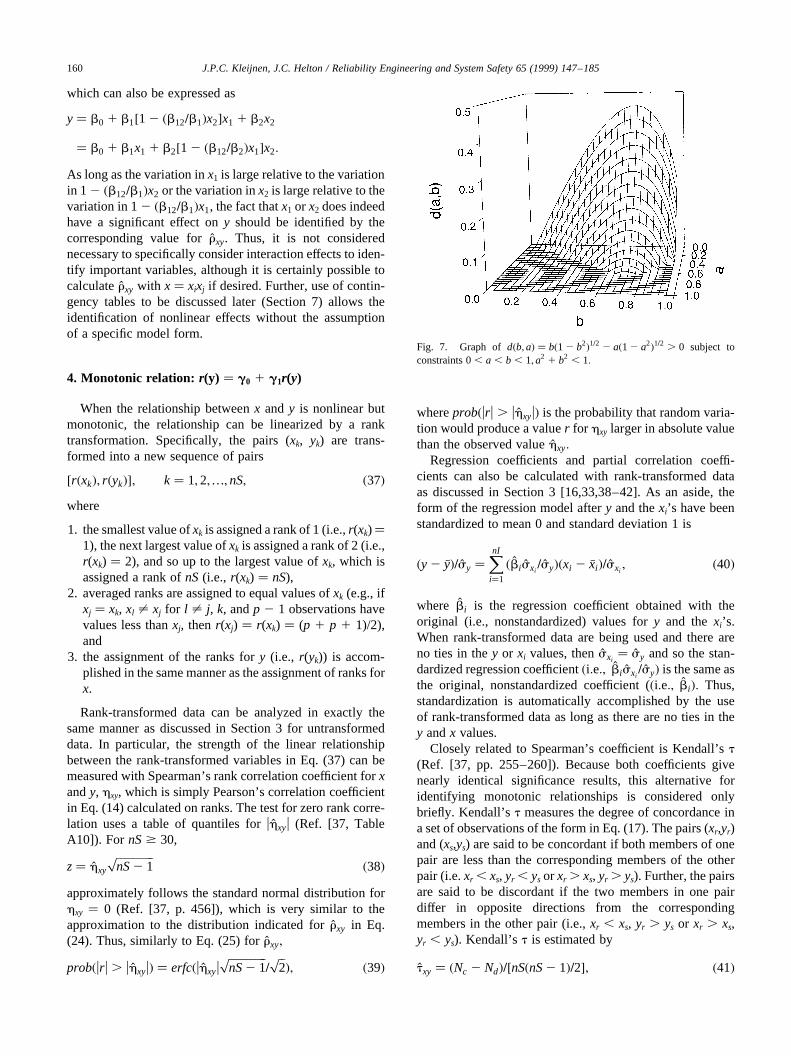
b�1 2 b2�1=2 . a�1 2 a2�1=2 �34�for a2 1 b2 , 1 anda , b (Fig. 7), an ordering of variableimportance based onu pxjyu , ubj u or u rxjyu produces thesame results when thexi are orthogonal; further, the valuesfor bj andrxjy will be the same and generally different frompxjy:
Owing to the conceptual simplicity of the sample correla-tion coefficientrxy and its close relationship to standardizedregression coefficients and partial correlation coefficients inthe presence of orthogonal values for thexi’s, this study willuse rxy to assess the strength of the linear relationshipbetweenx andy. In the presence of small deviations fromorthogonality (i.e., the existence of small correlationsbetween thexi), the three measures will still give similarresults. However, in the presence of large deviations fromorthogonality, the three measures can give quite different,and possibly misleading, indications of the effects of indi-vidual variables.
As noted earlier,rxy 8 0 should not be interpreted tomean that no relationship exists betweenx and y. Forexample,
y� b0xb1 �35�results in a low, but nonzero, value forrxy even though thereis no noise in the relationship betweenx andy. In this case, alogarithmic transformation will linearize the relationshipbetweenx and y. However, such transformations may notexist and, given that they do exist, identifying them is notalways easy. For example, logarithmic transformations arenot applicable when some of they values are zero, which is afairly common analysis situation. One possible transforma-tion of fairly broad applicability is the rank transformation,which is discussed in Section 4.
A possible complication in the use ofrxy to identify theexistence of a relationship betweenx andy can be the exis-tence of interactions with other variables. For example, therelationship betweeny, x1, andx2 might be of the form
y� b0 1 b1x1 1 b2x2 1 b12x1x2; �36�
J.P.C. Kleijnen, J.C. Helton / Reliability Engineering and System Safety 65 (1999) 147–185 159
which can also be expressed as
y� b0 1 b1�1 2 �b12=b1�x2�x1 1 b2x2
� b0 1 b1x1 1 b2�1 2 �b12=b2�x1�x2:
As long as the variation inx1 is large relative to the variationin 1 2 �b12=b1�x2 or the variation inx2 is large relative to thevariation in 12 �b12=b1�x1, the fact thatx1 or x2 does indeedhave a significant effect ony should be identified by thecorresponding value forrxy. Thus, it is not considerednecessary to specifically consider interaction effects to iden-tify important variables, although it is certainly possible tocalculaterxy with x� xixj if desired. Further, use of contin-gency tables to be discussed later (Section 7) allows theidentification of nonlinear effects without the assumptionof a specific model form.
4. Monotonic relation: r(y) � g0 1 g1r(y)
When the relationship betweenx andy is nonlinear butmonotonic, the relationship can be linearized by a ranktransformation. Specifically, the pairs (xk, yk) are trans-formed into a new sequence of pairs
�r�xk�; r�yk��; k � 1;2;…;nS; �37�where
1. the smallest value ofxk is assigned a rank of 1 (i.e.,r(xk)�1), the next largest value ofxk is assigned a rank of 2 (i.e.,r(xk) � 2), and so up to the largest value ofxk, which isassigned a rank ofnS(i.e., r(xk) � nS),
2. averaged ranks are assigned to equal values ofxk (e.g., ifxj � xk, xl ± xj for l ± j, k, andp 2 1 observations havevalues less thanxj, thenr(xj) � r(xk) � (p 1 p 1 1)/2),and
3. the assignment of the ranks fory (i.e., r(yk)) is accom-plished in the same manner as the assignment of ranks forx.
Rank-transformed data can be analyzed in exactly thesame manner as discussed in Section 3 for untransformeddata. In particular, the strength of the linear relationshipbetween the rank-transformed variables in Eq. (37) can bemeasured with Spearman’s rank correlation coefficient forxandy, hxy, which is simply Pearson’s correlation coefficientin Eq. (14) calculated on ranks. The test for zero rank corre-lation uses a table of quantiles foruhxyu (Ref. [37, TableA10]). For nS$ 30,
z� hxy
���������nS2 1p �38�
approximately follows the standard normal distribution forhxy � 0 (Ref. [37, p. 456]), which is very similar to theapproximation to the distribution indicated forrxy in Eq.(24). Thus, similarly to Eq. (25) forrxy;
prob�ur u . uhxyu� � erfc�uhxyu���������nS2 1p
=��2p �; �39�
whereprob�ur u . uhxyu� is the probability that random varia-tion would produce a valuer for hxy larger in absolute valuethan the observed valuehxy:
Regression coefficients and partial correlation coeffi-cients can also be calculated with rank-transformed dataas discussed in Section 3 [16,33,38–42]. As an aside, theform of the regression model aftery and thexi’s have beenstandardized to mean 0 and standard deviation 1 is
�y 2 �y�=sy �XnI
i�1
�bi sxi=sy��xi 2 �xi�=sxi
; �40�
where bi is the regression coefficient obtained with theoriginal (i.e., nonstandardized) values fory and thexi’s.When rank-transformed data are being used and there areno ties in they or xi values, thensxi
� sy and so the stan-dardized regression coefficient�i:e:; bisxi
=sy� is the same asthe original, nonstandardized coefficient (�i:e:; bi�: Thus,standardization is automatically accomplished by the useof rank-transformed data as long as there are no ties in they andx values.
Closely related to Spearman’s coefficient is Kendall’st(Ref. [37, pp. 255–260]). Because both coefficients givenearly identical significance results, this alternative foridentifying monotonic relationships is considered onlybriefly. Kendall’st measures the degree of concordance ina set of observations of the form in Eq. (17). The pairs (xr,yr)and (xs,ys) are said to be concordant if both members of onepair are less than the corresponding members of the otherpair (i.e.xr , xs, yr , ys or xr . xs, yr . ys). Further, the pairsare said to be discordant if the two members in one pairdiffer in opposite directions from the correspondingmembers in the other pair (i.e.,xr , xs, yr . ys or xr . xs,yr , ys). Kendall’st is estimated by
txy � �Nc 2 Nd�=�nS�nS2 1�=2�; �41�
J.P.C. Kleijnen, J.C. Helton / Reliability Engineering and System Safety 65 (1999) 147–185160
Fig. 7. Graph ofd�b; a� � b�1 2 b2�1=2 2 a�1 2 a2�1=2 . 0 subject toconstraints 0, a , b , 1;a2 1 b2 , 1:
whereNc is the number of concordant pairs of observations,Nd is the number of discordant pairs of observations, andnS(nS2 1)/2 is the total number of pairs {(xr,yr), (xs,ys)} ofobservations. The statistictxy has a distribution that isadequately approximated by the normal distribution forsample sizes as small asnS� 8. In contrast, larger samples(e.g.,nS $ 30) are required forhxy to approach a normaldistribution; fortunately, Monte Carlo sensitivity studiestypically use sample sizes larger thannS� 30. Becauseestimates for Spearman’s coefficienthxy and Kendall’stxy
produce similar rankings of monotonicity andhxy is moreintuitively appealing because of its close relationship toPearson’s coefficientrxy; this presentation will usehxy toidentify nonlinear but monotonic relationships in scatter-plots.
5. Location of y dependent onx
Tests for two distinct types of patterns in scatterplotswere considered in Sections 3 and 4, with the Pearson corre-lation coefficient used to identify linear patterns (Section 3)and the Spearman correlation coefficient used to identifynonlinear but monotonic patterns (Section 4). This sectionreviews tests for a broader class of patterns. Specifically,patterns are sought where some measure of central tendencyfor y changes with changing values forx. Linear and mono-tonic patterns have this characteristic; however, decidedlynonlinear and nonmonotonic patterns can also have thischaracteristic (e.g., see the scatterplot forBHPRM in Fig.6(d)).
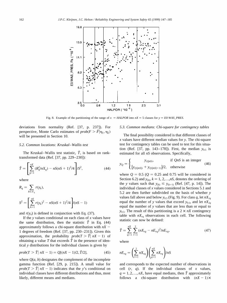
The approach taken is to divide the values forx (i.e.xk, k�1,2,…,nS) into nX classes and then to test to determine ifyhas a common measure of central tendency across theseclasses. Thus,x must be defined on at least a nominalscale to permit the definition of the necessary classes. Clas-sic measures of central tendency are the mean or expectedvalue,E(y), and the median,y0.5. The mean is a more widelyused measure of central tendency but the median is lesssensitive to outliers (e.g., see the Princeton robustnessstudy reported in Ref. [43]).
Most of thex’s under consideration are actually definedon an interval scale (see Table 2), and the required classesare obtained by subdividing the range ofx into a sequence ofmutually exclusive and exhaustive subintervals containingequal numbers of sampled values (Fig. 8). A fewx’s arediscrete with unequal probabilities for the individualxvalues (e.g., seeWMICDFLG in Fig. 3(a)); for these vari-ables, individual classes are defined for each of the distinctvalues. However, the optimum definition of the classes isnot at all apparent, and in practice, some experimentationmay be required to determine an appropriate division of thex values into classes.
For a given variablex and its nX associated classes,the following statistics will be used to identify apparent
deviations from a common central tendency:
1. the ANOVA F statistic for equal means, which requiresan interval scale fory (Section 5.1),
2. the Kruskal–Wallis test for common locations, whichrequires an ordinal scale fory (Section 5.2), and
3. the chi-square test for equal medians, which also requiresan ordinal scale fory (Section 5.3).
5.1. Common means: ANOVA F statistic
For notional convenience, letq, q� 1,2,…,nX, designatethe individual classes into which the values ofx have beendivided; letXq designate the set such thatk [ Xq only if xk
belongs to classq; and letnXq equal the number of elementscontained inXq (i.e., the number ofxk’s associated withclassq). The ANOVA F test is commonly used to test forequivalence of conditional means [44]:
F�nX 2 1; nS2 nX� �
PnX
q�1nXq �y
2q 2 nS�y2
" #=�nX 2 1�
PnS
k�1y2
k 2PnX
q�1nXq �y
2q
" #=�nS2 nX�
;
�42�wherenX 2 1 andnS2 nX are the number of degrees offreedom for the numerator and denominator, respectively,�yq �
Pk[Xq
yk=nXq; and �y is defined in conjunction with Eq.(14).
If the y values conditional on each class ofx values arenormally distributed with equal expected values, then thestatistic F (nX 2 1, nS 2 nX) in Eq. (42) follows anFdistribution with (nX 2 1, nS 2 nX) degrees of freedom.This is the most powerful test for equality of means giventhat the indicated normality assumptions hold [44]. Theprobability prob�F . Fuh1;h2� of exceeding anF statisticof value F calculated with (h1, h2) degrees of freedom canthen be estimated by
prob�F . Fuh1;h2� � Iv�h2=2;h1=2�; v� h2=�h2 1 h1F�;�43�
whereIv (a, b) designates the incomplete beta function (Ref.[29], p. 222).
Unfortunately, they values for each class may not followa normal distribution. Various goodness of fit tests (e.g., chi-square, Kolmogorov–Smirnov, Cramer–von Mises, Ander-son–Darling) can be used to test for normality of theyvalues (Ref. [45, pp. 94–95] and Ref. [46]). However, thenumber of observations per class (e.g., 30 or 60 for many ofthe variables considered in this study) may be too small toprovide a powerful test. If a goodness-of-fit test leads to arejection of the normality hypothesis, then it may be appro-priate to apply a normalizing transformation such as theBox–Cox transformation, which includes the logarithmictransformation as a special case (Ref. [45, pp. 175–185]).Fortunately, the ANOVAF test is robust with respect to
J.P.C. Kleijnen, J.C. Helton / Reliability Engineering and System Safety 65 (1999) 147–185 161
deviations from normality (Ref. [37, p. 237]). Forperspective, Monte Carlo estimates ofprob�F . Fuh1;h2�will be presented in Section 10.
5.2. Common locations: Kruskal–Wallis test
The Kruskal–Wallis test statistic,T, is based on rank-transformed data (Ref. [37, pp. 229–230]):
T �XnX
q�1
�R2q=nXq�2 nS�nS1 1�2=4
24 35=S2; �44�
where
Rq �X
k[Xq
r�yk�;
S2 �XnS
k�1
r�yk�2 2 nS�nS1 1�2=4" #
=�nS2 1�
andr(yk) is defined in conjunction with Eq. (37).If the y values conditional on each class ofx values have
the same distribution, then the statisticT in Eq. (44)approximately follows a chi-square distribution withnX 21 degrees of freedom (Ref. [37, pp. 230–231]). Given thisapproximation, the probabilityprob�T . Tu nX 2 1� ofobtaining a valueT that exceedsT in the presence of iden-tical y distributions for the individual classes is given by
prob�T . Tu nX 2 1� � Q��nX 2 1�=2; T=2�; �45�whereQ(a, b) designates the complement of the incompletegamma function (Ref. [29, p. 215]). A small value forprob�T . Tu nX 2 1� indicates that they’s conditional onindividual classes have different distributions and thus, mostlikely, different means and medians.
5.3. Common medians: Chi-square for contingency tables
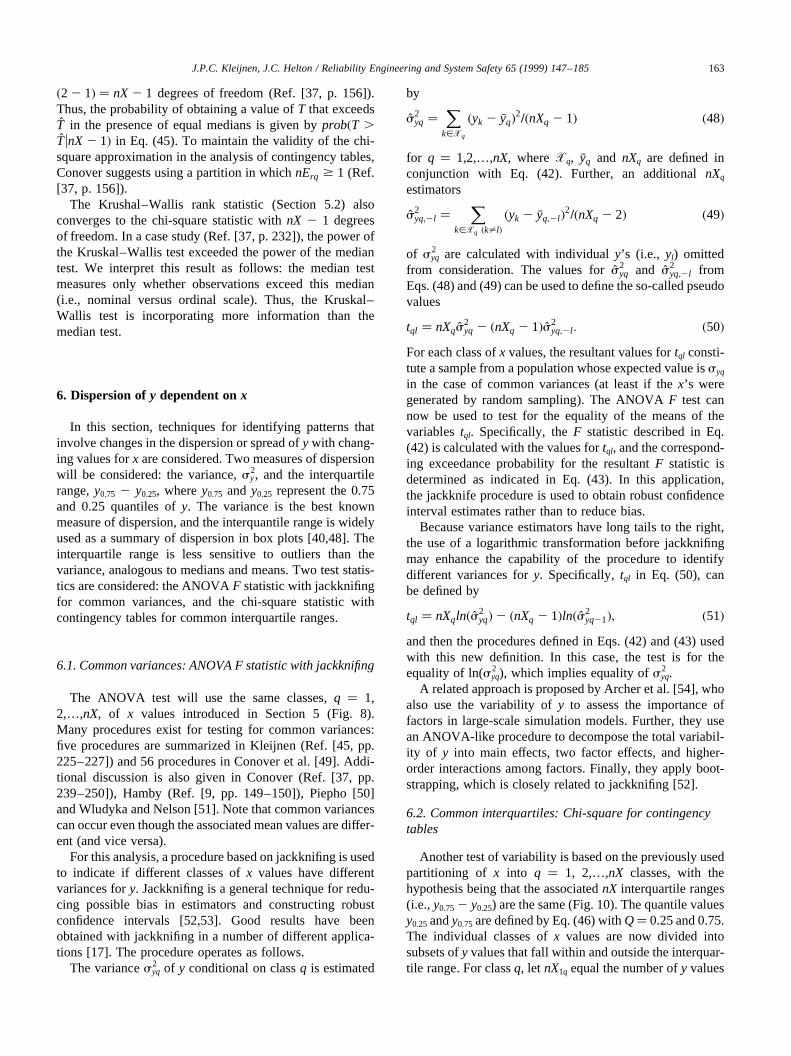
The final possibility considered is that different classes ofx values have different median values fory. The chi-squaretest for contingency tables can be used to test for this situa-tion (Ref. [37, pp. 143–178]). First, the mediany0.5 isestimated for allnSobservations. Specifically,
yQ �y�QnS�; if QnSis an integer
y��QnS�� 1 y��QnS�11�� �
=2; otherwise
(�46�
whereQ � 0.5 (Q � 0.25 and 0.75 will be considered inSection 6.2) andy(k), k� 1, 2,…,nS, denotes the ordering ofthe y values such thaty(k) # y(k11) (Ref. [47, p. 14]). Theindividual classes ofx values considered in Sections 5.1 and5.2 are then further subdivided on the basis of whetheryvalues fall above and belowy0.5 (Fig. 9). For classq, let nX1q
equal the number ofy values that exceedy0.5, and letnX2q
equal the number ofy values that are less than or equal toy0.5. The result of this partitioning is a 2× nX contingencytable with nXrq observations in each cell. The followingstatistic can now be defined:
T �XnX
q�1
X2r�1
�nXrq 2 nErq�2=nErq; �47�
where
nErq �X2r�1
nXrq
! XnX
q�1
nXrq
0@ 1A=nS
and corresponds to the expected number of observations incell (r, q). If the individual classes ofx values,q� 1;2;…; nX, have equal medians, thenT approximatelyfollows a chi-square distribution with �nX 2 1� �
J.P.C. Kleijnen, J.C. Helton / Reliability Engineering and System Safety 65 (1999) 147–185162
Fig. 8. Example of the partitioning of the range ofx � HALPORinto nX� 5 classes fory � E0:WAS_PRES.
�2 2 1� � nX 2 1 degrees of freedom (Ref. [37, p. 156]).Thus, the probability of obtaining a value ofT that exceedsT in the presence of equal medians is given byprob�T .TunX 2 1� in Eq. (45). To maintain the validity of the chi-square approximation in the analysis of contingency tables,Conover suggests using a partition in whichnErq $ 1 (Ref.[37, p. 156]).
The Krushal–Wallis rank statistic (Section 5.2) alsoconverges to the chi-square statistic withnX 2 1 degreesof freedom. In a case study (Ref. [37, p. 232]), the power ofthe Kruskal–Wallis test exceeded the power of the mediantest. We interpret this result as follows: the median testmeasures only whether observations exceed this median(i.e., nominal versus ordinal scale). Thus, the Kruskal–Wallis test is incorporating more information than themedian test.
6. Dispersion ofy dependent onx
In this section, techniques for identifying patterns thatinvolve changes in the dispersion or spread ofy with chang-ing values forx are considered. Two measures of dispersionwill be considered: the variance,s2
y, and the interquartilerange,y0.75 2 y0.25, wherey0.75 and y0.25 represent the 0.75and 0.25 quantiles ofy. The variance is the best knownmeasure of dispersion, and the interquantile range is widelyused as a summary of dispersion in box plots [40,48]. Theinterquartile range is less sensitive to outliers than thevariance, analogous to medians and means. Two test statis-tics are considered: the ANOVAF statistic with jackknifingfor common variances, and the chi-square statistic withcontingency tables for common interquartile ranges.
6.1. Common variances: ANOVA F statistic with jackknifing
The ANOVA test will use the same classes,q � 1,2,…,nX, of x values introduced in Section 5 (Fig. 8).Many procedures exist for testing for common variances:five procedures are summarized in Kleijnen (Ref. [45, pp.225–227]) and 56 procedures in Conover et al. [49]. Addi-tional discussion is also given in Conover (Ref. [37, pp.239–250]), Hamby (Ref. [9, pp. 149–150]), Piepho [50]and Wludyka and Nelson [51]. Note that common variancescan occur even though the associated mean values are differ-ent (and vice versa).
For this analysis, a procedure based on jackknifing is usedto indicate if different classes ofx values have differentvariances fory. Jackknifing is a general technique for redu-cing possible bias in estimators and constructing robustconfidence intervals [52,53]. Good results have beenobtained with jackknifing in a number of different applica-tions [17]. The procedure operates as follows.
The variances2yq of y conditional on classq is estimated
by
s2yq �
Xk[Xq
�yk 2 �yq�2=�nXq 2 1� �48�
for q � 1,2,…,nX, whereXq, �yq and nXq are defined inconjunction with Eq. (42). Further, an additionalnXq
estimators
s2yq;2l �
Xk[Xq �k±l�
�yk 2 �yq;2l�2=�nXq 2 2� �49�
of s2yq are calculated with individualy’s (i.e., yl) omitted
from consideration. The values fors2yq and s2
yq;2l fromEqs. (48) and (49) can be used to define the so-called pseudovalues
tql � nXqs2yq 2 �nXq 2 1�s2
yq;2l : �50�For each class ofx values, the resultant values fortql consti-tute a sample from a population whose expected value issyq
in the case of common variances (at least if thex’s weregenerated by random sampling). The ANOVAF test cannow be used to test for the equality of the means of thevariablestql. Specifically, theF statistic described in Eq.(42) is calculated with the values fortql, and the correspond-ing exceedance probability for the resultantF statistic isdetermined as indicated in Eq. (43). In this application,the jackknife procedure is used to obtain robust confidenceinterval estimates rather than to reduce bias.
Because variance estimators have long tails to the right,the use of a logarithmic transformation before jackknifingmay enhance the capability of the procedure to identifydifferent variances fory. Specifically,tql in Eq. (50), canbe defined by
tql � nXqln�s2yq�2 �nXq 2 1�ln�s2
yq21�; �51�and then the procedures defined in Eqs. (42) and (43) usedwith this new definition. In this case, the test is for theequality of ln(s2
yq), which implies equality ofs2yq.
A related approach is proposed by Archer et al. [54], whoalso use the variability ofy to assess the importance offactors in large-scale simulation models. Further, they usean ANOVA-like procedure to decompose the total variabil-ity of y into main effects, two factor effects, and higher-order interactions among factors. Finally, they apply boot-strapping, which is closely related to jackknifing [52].
6.2. Common interquartiles: Chi-square for contingencytables
Another test of variability is based on the previously usedpartitioning of x into q � 1, 2,…,nX classes, with thehypothesis being that the associatednX interquartile ranges(i.e.,y0.752 y0.25) are the same (Fig. 10). The quantile valuesy0.25andy0.75are defined by Eq. (46) withQ� 0.25 and 0.75.The individual classes ofx values are now divided intosubsets ofy values that fall within and outside the interquar-tile range. For classq, let nX1q equal the number ofy values
J.P.C. Kleijnen, J.C. Helton / Reliability Engineering and System Safety 65 (1999) 147–185 163
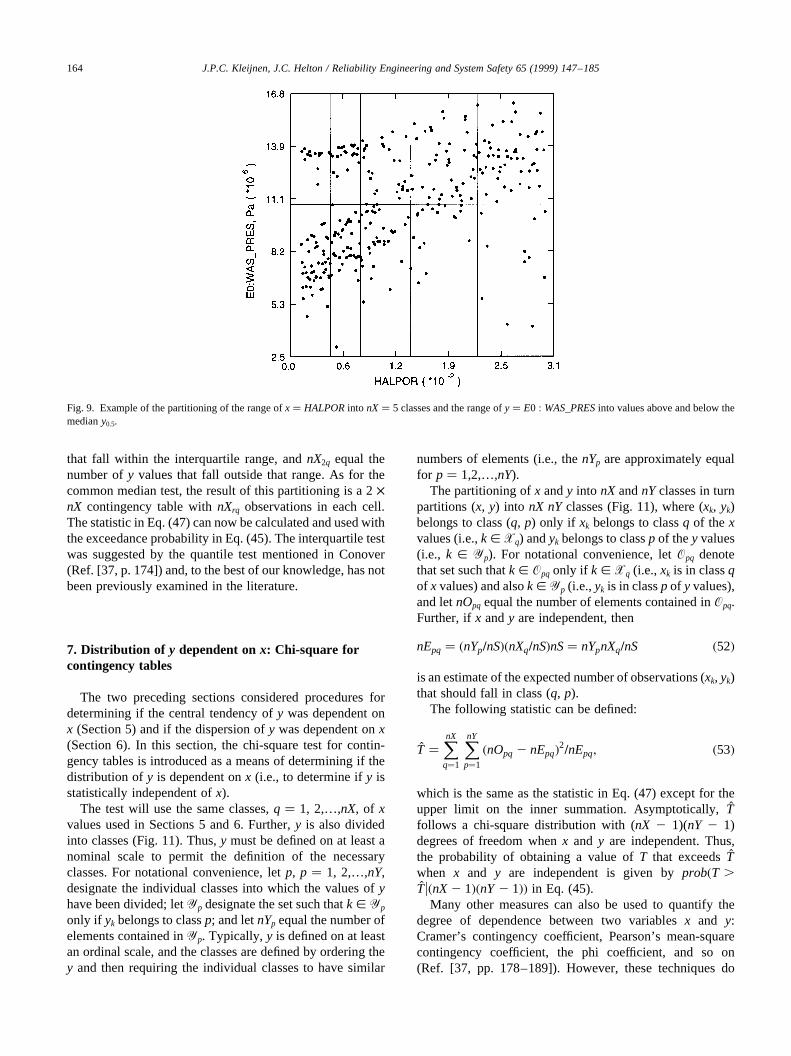
that fall within the interquartile range, andnX2q equal thenumber ofy values that fall outside that range. As for thecommon median test, the result of this partitioning is a 2×nX contingency table withnXrq observations in each cell.The statistic in Eq. (47) can now be calculated and used withthe exceedance probability in Eq. (45). The interquartile testwas suggested by the quantile test mentioned in Conover(Ref. [37, p. 174]) and, to the best of our knowledge, has notbeen previously examined in the literature.
7. Distribution of y dependent onx: Chi-square forcontingency tables
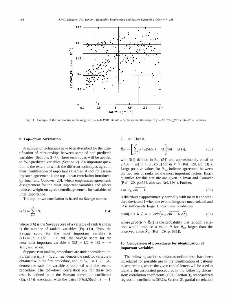
The two preceding sections considered procedures fordetermining if the central tendency ofy was dependent onx (Section 5) and if the dispersion ofy was dependent onx(Section 6). In this section, the chi-square test for contin-gency tables is introduced as a means of determining if thedistribution ofy is dependent onx (i.e., to determine ify isstatistically independent ofx).
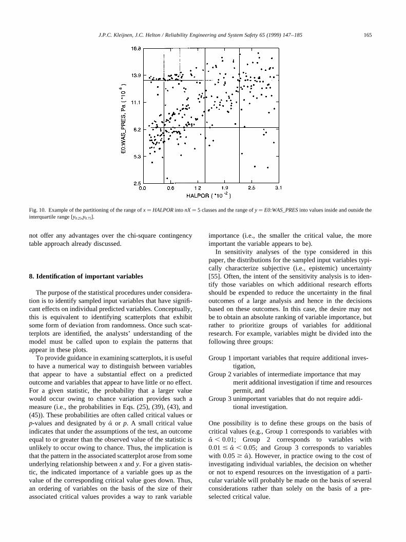
The test will use the same classes,q � 1, 2,…,nX, of xvalues used in Sections 5 and 6. Further,y is also dividedinto classes (Fig. 11). Thus,y must be defined on at least anominal scale to permit the definition of the necessaryclasses. For notational convenience, letp, p � 1, 2,…,nY,designate the individual classes into which the values ofyhave been divided; letYp designate the set such thatk [ Yp
only if yk belongs to classp; and letnYp equal the number ofelements contained inYp. Typically, y is defined on at leastan ordinal scale, and the classes are defined by ordering they and then requiring the individual classes to have similar
numbers of elements (i.e., thenYp are approximately equalfor p � 1,2,…,nY).
The partitioning ofx andy into nX andnYclasses in turnpartitions (x, y) into nX nYclasses (Fig. 11), where (xk, yk)belongs to class (q, p) only if xk belongs to classq of the xvalues (i.e.,k [ Xq) andyk belongs to classp of they values(i.e., k [ Yp). For notational convenience, letOpq denotethat set such thatk [ Opq only if k [ Xq (i.e.,xk is in classqof x values) and alsok [ Yp (i.e.,yk is in classp of y values),and letnOpq equal the number of elements contained inOpq.Further, ifx andy are independent, then
nEpq � �nYp=nS��nXq=nS�nS� nYpnXq=nS �52�
is an estimate of the expected number of observations (xk, yk)that should fall in class (q, p).
The following statistic can be defined:
T �XnX
q�1
XnY
p�1
�nOpq 2 nEpq�2=nEpq; �53�
which is the same as the statistic in Eq. (47) except for theupper limit on the inner summation. Asymptotically,Tfollows a chi-square distribution with (nX 2 1)(nY 2 1)degrees of freedom whenx and y are independent. Thus,the probability of obtaining a value ofT that exceedsTwhen x and y are independent is given byprob�T .Tu�nX 2 1��nY 2 1�� in Eq. (45).
Many other measures can also be used to quantify thedegree of dependence between two variablesx and y:Cramer’s contingency coefficient, Pearson’s mean-squarecontingency coefficient, the phi coefficient, and so on(Ref. [37, pp. 178–189]). However, these techniques do
J.P.C. Kleijnen, J.C. Helton / Reliability Engineering and System Safety 65 (1999) 147–185164
Fig. 9. Example of the partitioning of the range ofx� HALPORinto nX� 5 classes and the range ofy� E0 : WAS_PRESinto values above and below themediany0.5.
not offer any advantages over the chi-square contingencytable approach already discussed.
8. Identification of important variables
The purpose of the statistical procedures under considera-tion is to identify sampled input variables that have signifi-cant effects on individual predicted variables. Conceptually,this is equivalent to identifying scatterplots that exhibitsome form of deviation from randomness. Once such scat-terplots are identified, the analysts’ understanding of themodel must be called upon to explain the patterns thatappear in these plots.
To provide guidance in examining scatterplots, it is usefulto have a numerical way to distinguish between variablesthat appear to have a substantial effect on a predictedoutcome and variables that appear to have little or no effect.For a given statistic, the probability that a larger valuewould occur owing to chance variation provides such ameasure (i.e., the probabilities in Eqs. (25), (39), (43), and(45)). These probabilities are often called critical values orp-values and designated byaà or p. A small critical valueindicates that under the assumptions of the test, an outcomeequal to or greater than the observed value of the statistic isunlikely to occur owing to chance. Thus, the implication isthat the pattern in the associated scatterplot arose from someunderlying relationship betweenx andy. For a given statis-tic, the indicated importance of a variable goes up as thevalue of the corresponding critical value goes down. Thus,an ordering of variables on the basis of the size of theirassociated critical values provides a way to rank variable
importance (i.e., the smaller the critical value, the moreimportant the variable appears to be).
In sensitivity analyses of the type considered in thispaper, the distributions for the sampled input variables typi-cally characterize subjective (i.e., epistemic) uncertainty[55]. Often, the intent of the sensitivity analysis is to iden-tify those variables on which additional research effortsshould be expended to reduce the uncertainty in the finaloutcomes of a large analysis and hence in the decisionsbased on these outcomes. In this case, the desire may notbe to obtain an absolute ranking of variable importance, butrather to prioritize groups of variables for additionalresearch. For example, variables might be divided into thefollowing three groups:
Group 1 important variables that require additional inves-tigation,
Group 2 variables of intermediate importance that maymerit additional investigation if time and resourcespermit, and
Group 3 unimportant variables that do not require addi-tional investigation.
One possibility is to define these groups on the basis ofcritical values (e.g., Group 1 corresponds to variables witha , 0:01; Group 2 corresponds to variables with0:01 # a , 0:05; and Group 3 corresponds to variableswith 0:05 $ a). However, in practice owing to the cost ofinvestigating individual variables, the decision on whetheror not to expend resources on the investigation of a parti-cular variable will probably be made on the basis of severalconsiderations rather than solely on the basis of a pre-selected critical value.
J.P.C. Kleijnen, J.C. Helton / Reliability Engineering and System Safety 65 (1999) 147–185 165
Fig. 10. Example of the partitioning of the range ofx� HALPORinto nX� 5 classes and the range ofy� E0:WAS_PRESinto values inside and outside theinterquartile range [y0.25,y0.75].
9. Top–down correlation
A number of techniques have been described for the iden-tification of relationships between sampled and predictedvariables (Sections 3–7). These techniques will be appliedto four predicted variables (Section 2). An important ques-tion is the extent to which the different techniques agree intheir identification of important variables. A tool for assess-ing such agreement is the top–down correlation introducedby Iman and Conover [20], which emphasizes agreement/disagreement for the most important variables and placesreduced weight on agreement/disagreement for variables oflittle importance.
The top–down correlation is based on Savage scores:
S�h� �XnI
j�h
1=j; �54�
whereS(h) is the Savage score of a variable of rankh andnIis the number of ranked variables (Eq. (1)). Thus, theSavage score for the most important variable isS�1� � 1=1 1 1=2 1 …1 1=nI; the Savage score for thenext most important variable isS�2� � 1=2 1 1=3 1…11=nI; and so on.
Suppose two ranking procedures are under consideration.Further, leth1i ; i � 1;2;…;nI, denote the rank for variablexi
obtained with the first procedure, and leth2i, i � 1, 2,…,nI,denote the rank for variablexi obtained with the secondprocedure. The top–down correlationR12 for these twotests is defined to be the Pearson correlation coefficient(Eq. (14)) associated with the pairs [S(h1i),S(h2i)], i � 1,
2,…,nI. That is,
R12 �XnI
i�1
S�h1i�S�h2i�2 nI
" #=�nI 2 S�1��; �55�
with S(1) defined in Eq. (54) and approximately equal to2.4501 ln[nI 1 0.5)/6.5] fornI $ 7 (Ref. [20, Eq. (3)]).Large positive values forR 12 indicate agreement betweenthe two sets of ranks for the most important factors. Exactquantiles for this statistic are given in Iman and Conover(Ref. [20, p.355]; also see Ref. [56]). Further,
z� R12
��������nI 2 1p �56�
is distributed approximately normally with mean 0 and stan-dard deviation 1 when the two rankings are uncorrelated andnI is sufficiently large. Under these conditions.
prob R. R12
ÿ � � 0:5erfc R12
��������nI 2 1p
=��2p� �
; �57�whereprob R. R12
ÿ �is the probability that random varia-
tion would produce a valueR for R12 larger than theobserved valueR12 (Ref. [29, p. 631]).
10. Comparison of procedures for identification ofimportant variables
The following statistics and/or associated tests have beenintroduced for possible use in the identification of patternsin scatterplots, where the given capital letters will be used toidentify the associated procedures in the following discus-sion: correlation coefficients (CCs, Section 3), standardizedregression coefficients (SRCs, Section 3), partial correlation
J.P.C. Kleijnen, J.C. Helton / Reliability Engineering and System Safety 65 (1999) 147–185166
Fig. 11. Example of the partitioning of the range ofx � HALPORinto nX� 5 classes and the range ofy � E0:WAS_PRESinto nY� 5 classes.
coefficients (PCCs, Section 3), rank correlation coeffi-cients (RCCs, Section 4), standardized rank regressioncoefficients (SRRCs, Section 4), partial rank correlationcoefficients (PRCCs, Section 4), common means (CMNs,Section 5.1), common locations(CLs, Section 5.2), commonmedians (CMDs, Section 5.3), common variances (CVs,Section 6.1), common interquartile ranges (CIQ, Section6.2), and statistical independence (SI, Section 7). Further,the following dependent variables with different behaviorshave been introduced as examples:E0:WAS_PRES,E0:BRAALIC, E2:WAS_SATB, and E2:WAS_PRES(Section 2). The results of applying the indicated proceduresto these dependent variables are now discussed.
10.1. Repository pressure under undisturbed conditions: y�E0:WAS_PRES
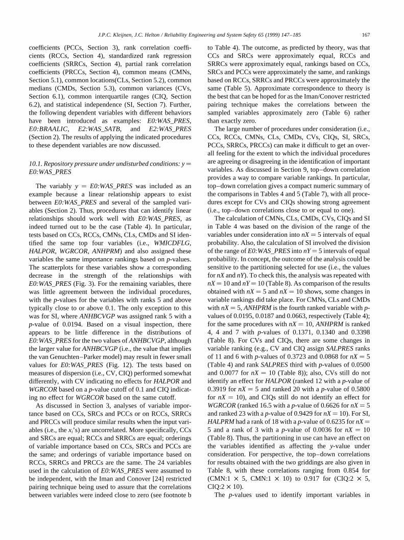
The variably y � E0:WAS_PRESwas included as anexample because a linear relationship appears to existbetweenE0:WAS_PRESand several of the sampled vari-ables (Section 2). Thus, procedures that can identify linearrelationships should work well withE0:WAS_PRES, asindeed turned out to be the case (Table 4). In particular,tests based on CCs, RCCs, CMNs, CLs, CMDs and SI iden-tified the same top four variables (i.e.,WMICDFLG,HALPOR, WGRCOR, ANHPRM) and also assigned thesevariables the same importance rankings based onp-values.The scatterplots for these variables show a correspondingdecrease in the strength of the relationships withE0:WAS_PRES(Fig. 3). For the remaining variables, therewas little agreement between the individual procedures,with the p-values for the variables with ranks 5 and abovetypically close to or above 0.1. The only exception to thiswas for SI, whereANHBCVGPwas assigned rank 5 with ap-value of 0.0194. Based on a visual inspection, thereappears to be little difference in the distributions ofE0:WAS_PRESfor the two values ofANHBCVGP, althoughthe larger value forANHBCVGP(i.e., the value that impliesthe van Genuchten–Parker model) may result in fewer smallvalues for E0:WAS_PRES(Fig. 12). The tests based onmeasures of dispersion (i.e., CV, CIQ) performed somewhatdifferently, with CV indicating no effects forHALPORandWGRCORbased on ap-value cutoff of 0.1 and CIQ indicat-ing no effect forWGRCORbased on the same cutoff.
As discussed in Section 3, analyses of variable impor-tance based on CCs, SRCs and PCCs or on RCCs, SRRCsand PRCCs will produce similar results when the input vari-ables (i.e., thexi’s) are uncorrelated. More specifically, CCsand SRCs are equal; RCCs and SRRCs are equal; orderingsof variable importance based on CCs, SRCs and PCCs arethe same; and orderings of variable importance based onRCCs, SRRCs and PRCCs are the same. The 24 variablesused in the calculation ofE0:WAS_PRESwere assumed tobe independent, with the Iman and Conover [24] restrictedpairing technique being used to assure that the correlationsbetween variables were indeed close to zero (see footnote b
to Table 4). The outcome, as predicted by theory, was thatCCs and SRCs were approximately equal, RCCs andSRRCs were approximately equal, rankings based on CCs,SRCs and PCCs were approximately the same, and rankingsbased on RCCs, SRRCs and PRCCs were approximately thesame (Table 5). Approximate correspondence to theory isthe best that can be hoped for as the Iman/Conover restrictedpairing technique makes the correlations between thesampled variables approximately zero (Table 6) ratherthan exactly zero.
The large number of procedures under consideration (i.e.,CCs, RCCs, CMNs, CLs, CMDs, CVs, CIQs, SI, SRCs,PCCs, SRRCs, PRCCs) can make it difficult to get an over-all feeling for the extent to which the individual proceduresare agreeing or disagreeing in the identification of importantvariables. As discussed in Section 9, top–down correlationprovides a way to compare variable rankings. In particular,top–down correlation gives a compact numeric summary ofthe comparisons in Tables 4 and 5 (Table 7), with all proce-dures except for CVs and CIQs showing strong agreement(i.e., top–down correlations close to or equal to one).
The calculation of CMNs, CLs, CMDs, CVs, CIQs and SIin Table 4 was based on the division of the range of thevariables under consideration intonX� 5 intervals of equalprobability. Also, the calculation of SI involved the divisionof the range ofE0:WAS_PRESinto nY� 5 intervals of equalprobability. In concept, the outcome of the analysis could besensitive to the partitioning selected for use (i.e., the valuesfor nXandnY). To check this, the analysis was repeated withnX� 10 andnY� 10 (Table 8). As comparison of the resultsobtained withnX� 5 andnX� 10 shows, some changes invariable rankings did take place. For CMNs, CLs and CMDswith nX� 5, ANHPRMis the fourth ranked variable withp-values of 0.0195, 0.0187 and 0.0663, respectively (Table 4);for the same procedures withnX� 10,ANHPRMis ranked4, 4 and 7 withp-values of 0.1371, 0.1340 and 0.3398(Table 8). For CVs and CIQs, there are some changes invariable ranking (e.g., CV and CIQ assignSALPRESranksof 11 and 6 withp-values of 0.3723 and 0.0868 fornX� 5(Table 4) and rankSALPRESthird with p-values of 0.0500and 0.0077 fornX � 10 (Table 8)); also, CVs still do notidentify an effect forHALPOR(ranked 12 with ap-value of0.3919 fornX� 5 and ranked 20 with ap-value of 0.5800for nX � 10), and CIQs still do not identify an effect forWGRCOR(ranked 16.5 with ap-value of 0.6626 fornX� 5and ranked 23 with ap-value of 0.9429 fornX� 10). For SI,HALPRMhad a rank of 18 with ap-value of 0.6235 fornX�5 and a rank of 3 with ap-value of 0.0036 fornX � 10(Table 8). Thus, the partitioning in use can have an effect onthe variables identified as affecting they-value underconsideration. For perspective, the top–down correlationsfor results obtained with the two griddings are also given inTable 8, with these correlations ranging from 0.854 for(CMN:1 × 5, CMN:1 × 10) to 0.917 for (CIQ:2× 5,CIQ:2 × 10).
The p-values used to identify important variables in
J.P.C. Kleijnen, J.C. Helton / Reliability Engineering and System Safety 65 (1999) 147–185 167
J.P.C. Kleijnen, J.C. Helton / Reliability Engineering and System Safety 65 (1999) 147–185168
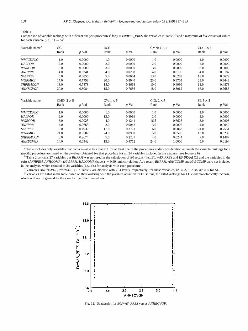
Table 4Comparison of variable rankings with different analysis proceduresa for y� E0:WAS_PRES, the variables in Table 2b and a maximum of five classes of valuesfor each variable (i.e.,nX� 5)c
Vairbale named CC RCC CMN: 1× 5 CL: 1 × 5Rank p-Val Rank p-Val Rank p-Val Rank p-Val
WMICDFLG 1.0 0.0000 1.0 0.0000 1.0 0.0000 1.0 0.0000HALPOR 2.0 0.0000 2.0 0.0000 2.0 0.0000 2.0 0.0000WGRCOR 3.0 0.0000 3.0 0.0000 3.0 0.0000 3.0 0.0000ANHPRM 4.0 0.0241 4.0 0.0268 4.0 0.0195 4.0 0.0187SALPRES 5.0 0.0855 5.0 0.0664 13.0 0.6283 13.0 0.5672WGRMICI 17.0 0.7753 20.0 0.8940 23.0 0.9705 23.0 0.9649SHPRMCON 18.0 0.7878 18.0 0.8618 10.0 0.4099 11.0 0.4878ANHBCVGP 20.0 0.8084 15.0 0.7686 18.0 0.8062 16.0 0.7686
Variable name CMD: 2× 5 CV: 1 × 5 CIQ: 2× 5 SI: 5× 5Rank p-Val Rank p-Val Rank p-Val Rank p-Val
WMICDFLG 1.0 0.0000 1.0 0.0000 1.0 0.0000 1.0 0.0000HALPOR 2.0 0.0000 12.0 0.3919 2.0 0.0000 2.0 0.0000WGRCOR 3.0 0.0025 4.0 0.1244 16.5 0.6626 3.0 0.0003ANHPRM 4.0 0.0663 2.0 0.0042 3.0 0.0007 4.0 0.0049SALPRES 9.0 0.4932 11.0 0.3723 6.0 0.0868 21.0 0.7554WGRMICI 24.0 0.9702 24.0 0.8900 5.0 0.0595 13.0 0.3239SHPRMCON 6.0 0.2674 5.0 0.1287 4.0 0.0244 7.0 0.1487ANHBCVGP 14.0 0.6442 13.0 0.4752 24.0 1.0000 5.0 0.0194
a Table includes only variables that had ap-value less than 0.1 for at least one of the procedures under consideration although the variable rankings for aspecific procedure are based on thep-values obtained for that procedure for all 24 variables included in the analysis (see footnote b).
b Table 2 contains 27 variables butBHPRMwas not used in the calculation of E0 results (i.e.,E0:WAS_PRESandE0:BRAALIC) and the variables in thepairs (ANHPRM, ANHCOMP), (HALPRM, HALCOMP) have a2 0.99 rank correlation. As a result,BHPRM, ANHCOMPandHALCOMPwere not includedin the analysis, which resulted in 24 variables (i.e.,x’s) for analysis with each procedure.
c VariablesANHBCVGP, WMICDFLG in Table 2 are discrete with 2, 3 levels, respectively: for these variables,nX� 2, 3. Also,nY� 5 for SI.d Variables are listed in the table based on their ordering with thep-values obtained for CCs: thus, the listed rankings for CCs will monotonically increase,
which will not in general be the case for the other procedures.
Fig. 12. Scatterplot forE0:WAS_PRESversusANHBCVGP.
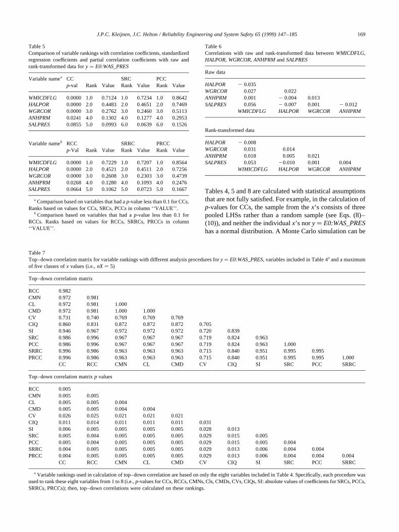
Tables 4, 5 and 8 are calculated with statistical assumptionsthat are not fully satisfied. For example, in the calculation ofp-values for CCs, the sample from thex’s consists of threepooled LHSs rather than a random sample (see Eqs. (8)–(10)), and neither the individualx’s nory� E0:WAS_PREShas a normal distribution. A Monte Carlo simulation can be
J.P.C. Kleijnen, J.C. Helton / Reliability Engineering and System Safety 65 (1999) 147–185 169
Table 6Correlations with raw and rank-transformed data betweenWMICDFLG,HALPOR, WGRCOR, ANHPRMandSALPRES
Raw data
HALPOR 2 0.035WGRCOR 0.027 0.022ANHPRM 0.001 2 0.004 0.013SALPRES 0.056 2 0.007 0.001 2 0.012
WMICDFLG HALPOR WGRCOR ANHPRM
Rank-transformed data
HALPOR 2 0.008WGRCOR 0.031 0.014ANHPRM 0.018 0.005 0.021SALPRES 0.053 20.010 0.001 0.004
WIMICDFLG HALPOR WGRCOR ANHPRM
Table 7Top–down correlation matrix for variable rankings with different analysis procedures fory� E0:WAS_PRES, variables included in Table 4a and a maximumof five classes ofx values (i.e.,nX� 5)
Top–down correlation matrix
RCC 0.982CMN 0.972 0.981CL 0.972 0.981 1.000CMD 0.972 0.981 1.000 1.000CV 0.731 0.740 0.769 0.769 0.769CIQ 0.860 0.831 0.872 0.872 0.872 0.705SI 0.946 0.967 0.972 0.972 0.972 0.720 0.839SRC 0.986 0.996 0.967 0.967 0.967 0.719 0.824 0.963PCC 0.986 0.996 0.967 0.967 0.967 0.719 0.824 0.963 1.000SRRC 0.996 0.986 0.963 0.963 0.963 0.715 0.840 0.951 0.995 0.995PRCC 0.996 0.986 0.963 0.963 0.963 0.715 0.840 0.951 0.995 0.995 1.000
CC RCC CMN CL CMD CV CIQ SI SRC PCC SRRC
Top–down correlation matrixp values
RCC 0.005CMN 0.005 0.005CL 0.005 0.005 0.004CMD 0.005 0.005 0.004 0.004CV 0.026 0.025 0.021 0.021 0.021CIQ 0.011 0.014 0.011 0.011 0.011 0.031SI 0.006 0.005 0.005 0.005 0.005 0.028 0.013SRC 0.005 0.004 0.005 0.005 0.005 0.029 0.015 0.005PCC 0.005 0.004 0.005 0.005 0.005 0.029 0.015 0.005 0.004SRRC 0.004 0.005 0.005 0.005 0.005 0.029 0.013 0.006 0.004 0.004PRCC 0.004 0.005 0.005 0.005 0.005 0.029 0.013 0.006 0.004 0.004 0.004
CC RCC CMN CL CMD CV CIQ SI SRC PCC SRRC
a Variable rankings used in calculation of top–down correlation are based on only the eight variables included in Table 4. Specifically, each procedurewasused to rank these eight variables from 1 to 8 (i.e.,p-values for CCs, RCCs, CMNs, Cls, CMDs, CVs, CIQs, SI: absolute values of coefficients for SRCs, PCCs,SRRCs, PRCCs); then, top–down correlations were calculated on these rankings.
Table 5Comparison of variable rankings with correlation coefficients, standardizedregression coefficients and partial correlation coefficients with raw andrank-transformed data fory � E0:WAS_PRES
Variable namea CC SRC PCCp-val Rank Value Rank Value Rank Value
WMICDFLG 0.0000 1.0 0.7124 1.0 0.7234 1.0 0.8642HALPOR 0.0000 2.0 0.4483 2.0 0.4651 2.0 0.7469WGRCOR 0.0000 3.0 0.2762 3.0 0.2460 3.0 0.5113ANHPRM 0.0241 4.0 0.1302 4.0 0.1277 4.0 0.2953SALPRES 0.0855 5.0 0.0993 6.0 0.0639 6.0 0.1526
Variable nameb RCC SRRC PRCCp-Val Rank Value Rank Value Rank Value
WMICDFLG 0.0000 1.0 0.7229 1.0 0.7207 1.0 0.8564HALPOR 0.0000 2.0 0.4521 2.0 0.4511 2.0 0.7256WGRCOR 0.0000 3.0 0.2608 3.0 0.2303 3.0 0.4739ANHPRM 0.0268 4.0 0.1280 4.0 0.1093 4.0 0.2476SALPRES 0.0664 5.0 0.1062 5.0 0.0723 5.0 0.1667
a Comparison based on variables that had ap-value less than 0.1 for CCs.Ranks based on values for CCs, SRCs, PCCs in column ‘‘VALUE’’.
b Comparison based on variables that had ap-value less than 0.1 forRCCs. Ranks based on values for RCCs, SRRCs, PRCCs in column‘‘VALUE’’.
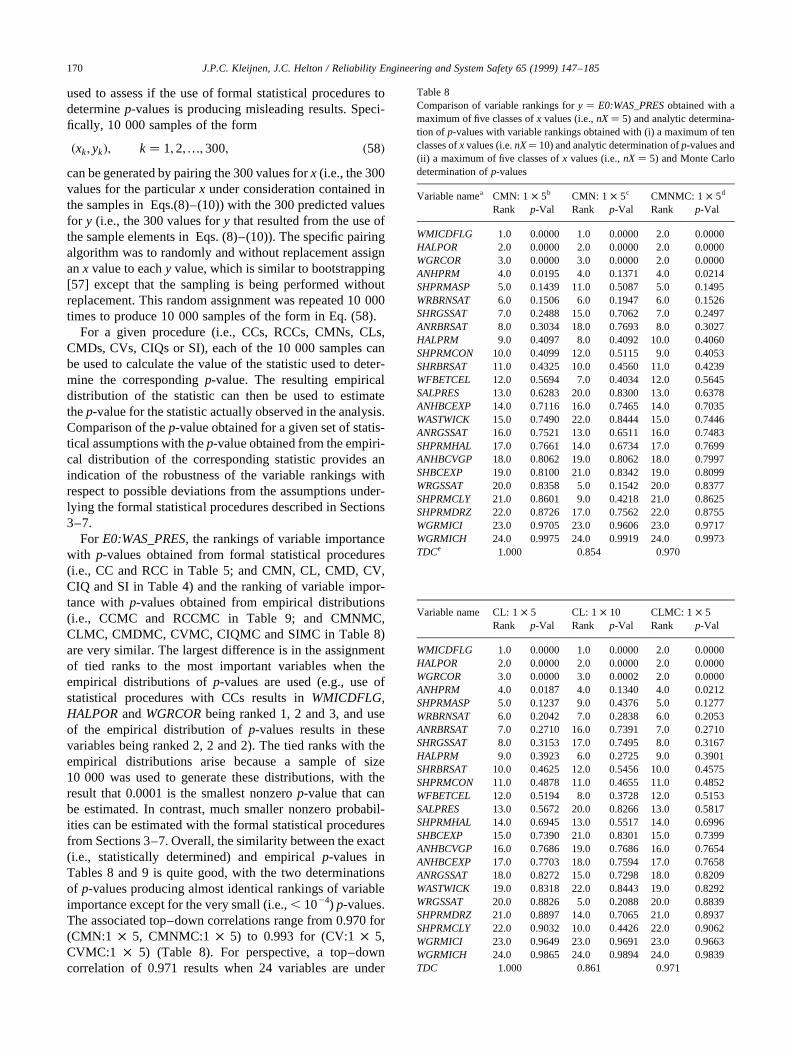
used to assess if the use of formal statistical procedures todeterminep-values is producing misleading results. Speci-fically, 10 000 samples of the form
�xk; yk�; k � 1;2;…;300; �58�can be generated by pairing the 300 values forx (i.e., the 300values for the particularx under consideration contained inthe samples in Eqs.(8)–(10)) with the 300 predicted valuesfor y (i.e., the 300 values fory that resulted from the use ofthe sample elements in Eqs. (8)–(10)). The specific pairingalgorithm was to randomly and without replacement assignanx value to eachy value, which is similar to bootstrapping[57] except that the sampling is being performed withoutreplacement. This random assignment was repeated 10 000times to produce 10 000 samples of the form in Eq. (58).
For a given procedure (i.e., CCs, RCCs, CMNs, CLs,CMDs, CVs, CIQs or SI), each of the 10 000 samples canbe used to calculate the value of the statistic used to deter-mine the correspondingp-value. The resulting empiricaldistribution of the statistic can then be used to estimatethep-value for the statistic actually observed in the analysis.Comparison of thep-value obtained for a given set of statis-tical assumptions with thep-value obtained from the empiri-cal distribution of the corresponding statistic provides anindication of the robustness of the variable rankings withrespect to possible deviations from the assumptions under-lying the formal statistical procedures described in Sections3–7.
For E0:WAS_PRES, the rankings of variable importancewith p-values obtained from formal statistical procedures(i.e., CC and RCC in Table 5; and CMN, CL, CMD, CV,CIQ and SI in Table 4) and the ranking of variable impor-tance withp-values obtained from empirical distributions(i.e., CCMC and RCCMC in Table 9; and CMNMC,CLMC, CMDMC, CVMC, CIQMC and SIMC in Table 8)are very similar. The largest difference is in the assignmentof tied ranks to the most important variables when theempirical distributions ofp-values are used (e.g., use ofstatistical procedures with CCs results inWMICDFLG,HALPORandWGRCORbeing ranked 1, 2 and 3, and useof the empirical distribution ofp-values results in thesevariables being ranked 2, 2 and 2). The tied ranks with theempirical distributions arise because a sample of size10 000 was used to generate these distributions, with theresult that 0.0001 is the smallest nonzerop-value that canbe estimated. In contrast, much smaller nonzero probabil-ities can be estimated with the formal statistical proceduresfrom Sections 3–7. Overall, the similarity between the exact(i.e., statistically determined) and empiricalp-values inTables 8 and 9 is quite good, with the two determinationsof p-values producing almost identical rankings of variableimportance except for the very small (i.e.,, 1024) p-values.The associated top–down correlations range from 0.970 for(CMN:1 × 5, CMNMC:1 × 5) to 0.993 for (CV:1× 5,CVMC:1 × 5) (Table 8). For perspective, a top–downcorrelation of 0.971 results when 24 variables are under
J.P.C. Kleijnen, J.C. Helton / Reliability Engineering and System Safety 65 (1999) 147–185170
Table 8Comparison of variable rankings fory � E0:WAS_PRESobtained with amaximum of five classes ofx values (i.e.,nX� 5) and analytic determina-tion of p-values with variable rankings obtained with (i) a maximum of tenclasses ofx values (i.e.nX� 10) and analytic determination ofp-values and(ii) a maximum of five classes ofx values (i.e.,nX� 5) and Monte Carlodetermination ofp-values
Variable namea CMN: 1 × 5b CMN: 1 × 5c CMNMC: 1 × 5d
Rank p-Val Rank p-Val Rank p-Val
WMICDFLG 1.0 0.0000 1.0 0.0000 2.0 0.0000HALPOR 2.0 0.0000 2.0 0.0000 2.0 0.0000WGRCOR 3.0 0.0000 3.0 0.0000 2.0 0.0000ANHPRM 4.0 0.0195 4.0 0.1371 4.0 0.0214SHPRMASP 5.0 0.1439 11.0 0.5087 5.0 0.1495WRBRNSAT 6.0 0.1506 6.0 0.1947 6.0 0.1526SHRGSSAT 7.0 0.2488 15.0 0.7062 7.0 0.2497ANRBRSAT 8.0 0.3034 18.0 0.7693 8.0 0.3027HALPRM 9.0 0.4097 8.0 0.4092 10.0 0.4060SHPRMCON 10.0 0.4099 12.0 0.5115 9.0 0.4053SHRBRSAT 11.0 0.4325 10.0 0.4560 11.0 0.4239WFBETCEL 12.0 0.5694 7.0 0.4034 12.0 0.5645SALPRES 13.0 0.6283 20.0 0.8300 13.0 0.6378ANHBCEXP 14.0 0.7116 16.0 0.7465 14.0 0.7035WASTWICK 15.0 0.7490 22.0 0.8444 15.0 0.7446ANRGSSAT 16.0 0.7521 13.0 0.6511 16.0 0.7483SHPRMHAL 17.0 0.7661 14.0 0.6734 17.0 0.7699ANHBCVGP 18.0 0.8062 19.0 0.8062 18.0 0.7997SHBCEXP 19.0 0.8100 21.0 0.8342 19.0 0.8099WRGSSAT 20.0 0.8358 5.0 0.1542 20.0 0.8377SHPRMCLY 21.0 0.8601 9.0 0.4218 21.0 0.8625SHPRMDRZ 22.0 0.8726 17.0 0.7562 22.0 0.8755WGRMICI 23.0 0.9705 23.0 0.9606 23.0 0.9717WGRMICH 24.0 0.9975 24.0 0.9919 24.0 0.9973TDCe 1.000 0.854 0.970
Variable name CL: 1× 5 CL: 1 × 10 CLMC: 1× 5Rank p-Val Rank p-Val Rank p-Val
WMICDFLG 1.0 0.0000 1.0 0.0000 2.0 0.0000HALPOR 2.0 0.0000 2.0 0.0000 2.0 0.0000WGRCOR 3.0 0.0000 3.0 0.0002 2.0 0.0000ANHPRM 4.0 0.0187 4.0 0.1340 4.0 0.0212SHPRMASP 5.0 0.1237 9.0 0.4376 5.0 0.1277WRBRNSAT 6.0 0.2042 7.0 0.2838 6.0 0.2053ANRBRSAT 7.0 0.2710 16.0 0.7391 7.0 0.2710SHRGSSAT 8.0 0.3153 17.0 0.7495 8.0 0.3167HALPRM 9.0 0.3923 6.0 0.2725 9.0 0.3901SHRBRSAT 10.0 0.4625 12.0 0.5456 10.0 0.4575SHPRMCON 11.0 0.4878 11.0 0.4655 11.0 0.4852WFBETCEL 12.0 0.5194 8.0 0.3728 12.0 0.5153SALPRES 13.0 0.5672 20.0 0.8266 13.0 0.5817SHPRMHAL 14.0 0.6945 13.0 0.5517 14.0 0.6996SHBCEXP 15.0 0.7390 21.0 0.8301 15.0 0.7399ANHBCVGP 16.0 0.7686 19.0 0.7686 16.0 0.7654ANHBCEXP 17.0 0.7703 18.0 0.7594 17.0 0.7658ANRGSSAT 18.0 0.8272 15.0 0.7298 18.0 0.8209WASTWICK 19.0 0.8318 22.0 0.8443 19.0 0.8292WRGSSAT 20.0 0.8826 5.0 0.2088 20.0 0.8839SHPRMDRZ 21.0 0.8897 14.0 0.7065 21.0 0.8937SHPRMCLY 22.0 0.9032 10.0 0.4426 22.0 0.9062WGRMICI 23.0 0.9649 23.0 0.9691 23.0 0.9663WGRMICH 24.0 0.9865 24.0 0.9894 24.0 0.9839TDC 1.000 0.861 0.971
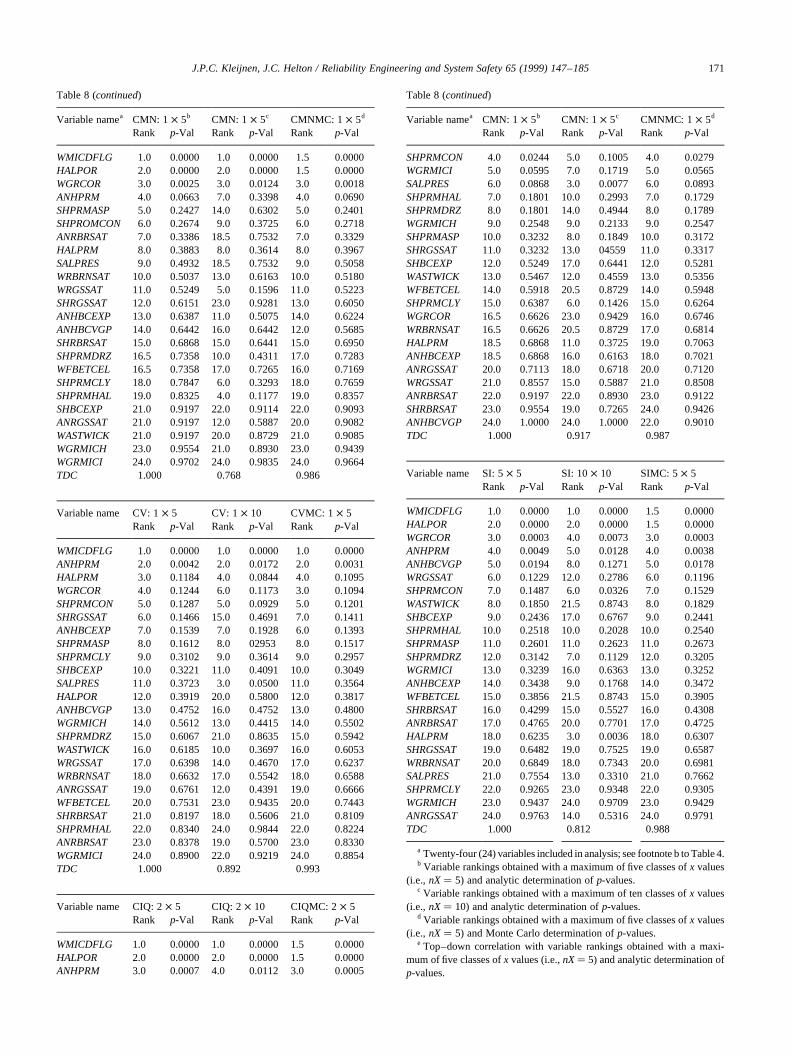
J.P.C. Kleijnen, J.C. Helton / Reliability Engineering and System Safety 65 (1999) 147–185 171
Table 8 (continued)
Variable namea CMN: 1 × 5b CMN: 1 × 5c CMNMC: 1 × 5d
Rank p-Val Rank p-Val Rank p-Val
WMICDFLG 1.0 0.0000 1.0 0.0000 1.5 0.0000HALPOR 2.0 0.0000 2.0 0.0000 1.5 0.0000WGRCOR 3.0 0.0025 3.0 0.0124 3.0 0.0018ANHPRM 4.0 0.0663 7.0 0.3398 4.0 0.0690SHPRMASP 5.0 0.2427 14.0 0.6302 5.0 0.2401SHPROMCON 6.0 0.2674 9.0 0.3725 6.0 0.2718ANRBRSAT 7.0 0.3386 18.5 0.7532 7.0 0.3329HALPRM 8.0 0.3883 8.0 0.3614 8.0 0.3967SALPRES 9.0 0.4932 18.5 0.7532 9.0 0.5058WRBRNSAT 10.0 0.5037 13.0 0.6163 10.0 0.5180WRGSSAT 11.0 0.5249 5.0 0.1596 11.0 0.5223SHRGSSAT 12.0 0.6151 23.0 0.9281 13.0 0.6050ANHBCEXP 13.0 0.6387 11.0 0.5075 14.0 0.6224ANHBCVGP 14.0 0.6442 16.0 0.6442 12.0 0.5685SHRBRSAT 15.0 0.6868 15.0 0.6441 15.0 0.6950SHPRMDRZ 16.5 0.7358 10.0 0.4311 17.0 0.7283WFBETCEL 16.5 0.7358 17.0 0.7265 16.0 0.7169SHPRMCLY 18.0 0.7847 6.0 0.3293 18.0 0.7659SHPRMHAL 19.0 0.8325 4.0 0.1177 19.0 0.8357SHBCEXP 21.0 0.9197 22.0 0.9114 22.0 0.9093ANRGSSAT 21.0 0.9197 12.0 0.5887 20.0 0.9082WASTWICK 21.0 0.9197 20.0 0.8729 21.0 0.9085WGRMICH 23.0 0.9554 21.0 0.8930 23.0 0.9439WGRMICI 24.0 0.9702 24.0 0.9835 24.0 0.9664TDC 1.000 0.768 0.986
Variable name CV: 1× 5 CV: 1 × 10 CVMC: 1× 5Rank p-Val Rank p-Val Rank p-Val
WMICDFLG 1.0 0.0000 1.0 0.0000 1.0 0.0000ANHPRM 2.0 0.0042 2.0 0.0172 2.0 0.0031HALPRM 3.0 0.1184 4.0 0.0844 4.0 0.1095WGRCOR 4.0 0.1244 6.0 0.1173 3.0 0.1094SHPRMCON 5.0 0.1287 5.0 0.0929 5.0 0.1201SHRGSSAT 6.0 0.1466 15.0 0.4691 7.0 0.1411ANHBCEXP 7.0 0.1539 7.0 0.1928 6.0 0.1393SHPRMASP 8.0 0.1612 8.0 02953 8.0 0.1517SHPRMCLY 9.0 0.3102 9.0 0.3614 9.0 0.2957SHBCEXP 10.0 0.3221 11.0 0.4091 10.0 0.3049SALPRES 11.0 0.3723 3.0 0.0500 11.0 0.3564HALPOR 12.0 0.3919 20.0 0.5800 12.0 0.3817ANHBCVGP 13.0 0.4752 16.0 0.4752 13.0 0.4800WGRMICH 14.0 0.5612 13.0 0.4415 14.0 0.5502SHPRMDRZ 15.0 0.6067 21.0 0.8635 15.0 0.5942WASTWICK 16.0 0.6185 10.0 0.3697 16.0 0.6053WRGSSAT 17.0 0.6398 14.0 0.4670 17.0 0.6237WRBRNSAT 18.0 0.6632 17.0 0.5542 18.0 0.6588ANRGSSAT 19.0 0.6761 12.0 0.4391 19.0 0.6666WFBETCEL 20.0 0.7531 23.0 0.9435 20.0 0.7443SHRBRSAT 21.0 0.8197 18.0 0.5606 21.0 0.8109SHPRMHAL 22.0 0.8340 24.0 0.9844 22.0 0.8224ANRBRSAT 23.0 0.8378 19.0 0.5700 23.0 0.8330WGRMICI 24.0 0.8900 22.0 0.9219 24.0 0.8854TDC 1.000 0.892 0.993
Variable name CIQ: 2× 5 CIQ: 2× 10 CIQMC: 2× 5Rank p-Val Rank p-Val Rank p-Val
WMICDFLG 1.0 0.0000 1.0 0.0000 1.5 0.0000HALPOR 2.0 0.0000 2.0 0.0000 1.5 0.0000ANHPRM 3.0 0.0007 4.0 0.0112 3.0 0.0005
Table 8 (continued)
Variable namea CMN: 1 × 5b CMN: 1 × 5c CMNMC: 1 × 5d
Rank p-Val Rank p-Val Rank p-Val
SHPRMCON 4.0 0.0244 5.0 0.1005 4.0 0.0279WGRMICI 5.0 0.0595 7.0 0.1719 5.0 0.0565SALPRES 6.0 0.0868 3.0 0.0077 6.0 0.0893SHPRMHAL 7.0 0.1801 10.0 0.2993 7.0 0.1729SHPRMDRZ 8.0 0.1801 14.0 0.4944 8.0 0.1789WGRMICH 9.0 0.2548 9.0 0.2133 9.0 0.2547SHPRMASP 10.0 0.3232 8.0 0.1849 10.0 0.3172SHRGSSAT 11.0 0.3232 13.0 04559 11.0 0.3317SHBCEXP 12.0 0.5249 17.0 0.6441 12.0 0.5281WASTWICK 13.0 0.5467 12.0 0.4559 13.0 0.5356WFBETCEL 14.0 0.5918 20.5 0.8729 14.0 0.5948SHPRMCLY 15.0 0.6387 6.0 0.1426 15.0 0.6264WGRCOR 16.5 0.6626 23.0 0.9429 16.0 0.6746WRBRNSAT 16.5 0.6626 20.5 0.8729 17.0 0.6814HALPRM 18.5 0.6868 11.0 0.3725 19.0 0.7063ANHBCEXP 18.5 0.6868 16.0 0.6163 18.0 0.7021ANRGSSAT 20.0 0.7113 18.0 0.6718 20.0 0.7120WRGSSAT 21.0 0.8557 15.0 0.5887 21.0 0.8508ANRBRSAT 22.0 0.9197 22.0 0.8930 23.0 0.9122SHRBRSAT 23.0 0.9554 19.0 0.7265 24.0 0.9426ANHBCVGP 24.0 1.0000 24.0 1.0000 22.0 0.9010TDC 1.000 0.917 0.987
Variable name SI: 5× 5 SI: 10× 10 SIMC: 5× 5Rank p-Val Rank p-Val Rank p-Val
WMICDFLG 1.0 0.0000 1.0 0.0000 1.5 0.0000HALPOR 2.0 0.0000 2.0 0.0000 1.5 0.0000WGRCOR 3.0 0.0003 4.0 0.0073 3.0 0.0003ANHPRM 4.0 0.0049 5.0 0.0128 4.0 0.0038ANHBCVGP 5.0 0.0194 8.0 0.1271 5.0 0.0178WRGSSAT 6.0 0.1229 12.0 0.2786 6.0 0.1196SHPRMCON 7.0 0.1487 6.0 0.0326 7.0 0.1529WASTWICK 8.0 0.1850 21.5 0.8743 8.0 0.1829SHBCEXP 9.0 0.2436 17.0 0.6767 9.0 0.2441SHPRMHAL 10.0 0.2518 10.0 0.2028 10.0 0.2540SHPRMASP 11.0 0.2601 11.0 0.2623 11.0 0.2673SHPRMDRZ 12.0 0.3142 7.0 0.1129 12.0 0.3205WGRMICI 13.0 0.3239 16.0 0.6363 13.0 0.3252ANHBCEXP 14.0 0.3438 9.0 0.1768 14.0 0.3472WFBETCEL 15.0 0.3856 21.5 0.8743 15.0 0.3905SHRBRSAT 16.0 0.4299 15.0 0.5527 16.0 0.4308ANRBRSAT 17.0 0.4765 20.0 0.7701 17.0 0.4725HALPRM 18.0 0.6235 3.0 0.0036 18.0 0.6307SHRGSSAT 19.0 0.6482 19.0 0.7525 19.0 0.6587WRBRNSAT 20.0 0.6849 18.0 0.7343 20.0 0.6981SALPRES 21.0 0.7554 13.0 0.3310 21.0 0.7662SHPRMCLY 22.0 0.9265 23.0 0.9348 22.0 0.9305WGRMICH 23.0 0.9437 24.0 0.9709 23.0 0.9429ANRGSSAT 24.0 0.9763 14.0 0.5316 24.0 0.9791TDC 1.000 0.812 0.988
a Twenty-four (24) variables included in analysis; see footnote b to Table 4.b Variable rankings obtained with a maximum of five classes ofx values
(i.e., nX� 5) and analytic determination ofp-values.c Variable rankings obtained with a maximum of ten classes ofx values
(i.e., nX� 10) and analytic determination ofp-values.d Variable rankings obtained with a maximum of five classes ofx values
(i.e., nX� 5) and Monte Carlo determination ofp-values.e Top–down correlation with variable rankings obtained with a maxi-
mum of five classes ofx values (i.e.,nX� 5) and analytic determination ofp-values.
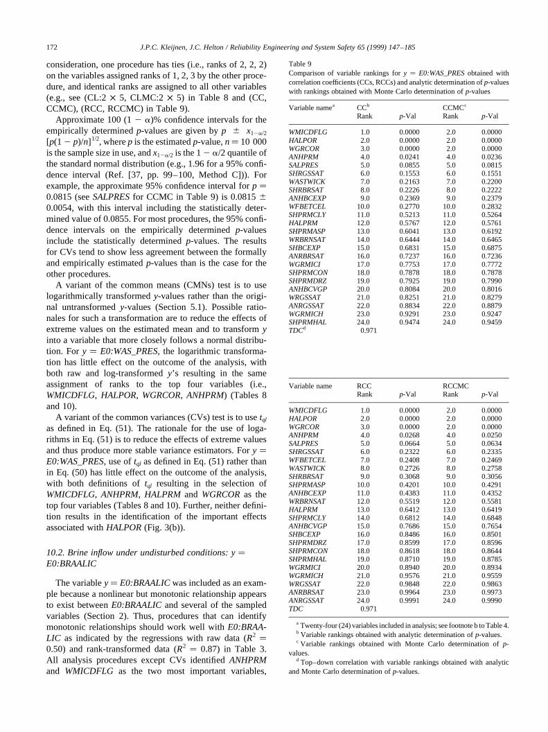
consideration, one procedure has ties (i.e., ranks of 2, 2, 2)on the variables assigned ranks of 1, 2, 3 by the other proce-dure, and identical ranks are assigned to all other variables(e.g., see (CL:2× 5, CLMC:2 × 5) in Table 8 and (CC,CCMC), (RCC, RCCMC) in Table 9).
Approximate 100 (12 a)% confidence intervals for theempirically determinedp-values are given byp ^ x12a/2
[p(1 2 p)/n] 1/2, wherep is the estimatedp-value,n� 10 000is the sample size in use, andx12a/2 is the 12 a/2 quantile ofthe standard normal distribution (e.g., 1.96 for a 95% confi-dence interval (Ref. [37, pp. 99–100, Method C])). Forexample, the approximate 95% confidence interval forp �0.0815 (seeSALPRESfor CCMC in Table 9) is 0.08150.0054, with this interval including the statistically deter-mined value of 0.0855. For most procedures, the 95% confi-dence intervals on the empirically determinedp-valuesinclude the statistically determinedp-values. The resultsfor CVs tend to show less agreement between the formallyand empirically estimatedp-values than is the case for theother procedures.
A variant of the common means (CMNs) test is to uselogarithmically transformedy-values rather than the origi-nal untransformedy-values (Section 5.1). Possible ratio-nales for such a transformation are to reduce the effects ofextreme values on the estimated mean and to transformyinto a variable that more closely follows a normal distribu-tion. For y � E0:WAS_PRES, the logarithmic transforma-tion has little effect on the outcome of the analysis, withboth raw and log-transformedy’s resulting in the sameassignment of ranks to the top four variables (i.e.,WMICDFLG, HALPOR, WGRCOR, ANHPRM) (Tables 8and 10).
A variant of the common variances (CVs) test is to usetql
as defined in Eq. (51). The rationale for the use of loga-rithms in Eq. (51) is to reduce the effects of extreme valuesand thus produce more stable variance estimators. Fory �E0:WAS_PRES, use oftql as defined in Eq. (51) rather thanin Eq. (50) has little effect on the outcome of the analysis,with both definitions oftql resulting in the selection ofWMICDFLG, ANHPRM, HALPRM and WGRCORas thetop four variables (Tables 8 and 10). Further, neither defini-tion results in the identification of the important effectsassociated withHALPOR(Fig. 3(b)).
10.2. Brine inflow under undisturbed conditions: y�E0:BRAALIC
The variabley� E0:BRAALICwas included as an exam-ple because a nonlinear but monotonic relationship appearsto exist betweenE0:BRAALICand several of the sampledvariables (Section 2). Thus, procedures that can identifymonotonic relationships should work well withE0:BRAA-LIC as indicated by the regressions with raw data (R2 �0.50) and rank-transformed data (R2 � 0.87) in Table 3.All analysis procedures except CVs identifiedANHPRMand WMICDFLG as the two most important variables,
J.P.C. Kleijnen, J.C. Helton / Reliability Engineering and System Safety 65 (1999) 147–185172
Table 9Comparison of variable rankings fory � E0:WAS_PRESobtained withcorrelation coefficients (CCs, RCCs) and analytic determination ofp-valueswith rankings obtained with Monte Carlo determination ofp-values
Variable namea CCb CCMCc
Rank p-Val Rank p-Val
WMICDFLG 1.0 0.0000 2.0 0.0000HALPOR 2.0 0.0000 2.0 0.0000WGRCOR 3.0 0.0000 2.0 0.0000ANHPRM 4.0 0.0241 4.0 0.0236SALPRES 5.0 0.0855 5.0 0.0815SHRGSSAT 6.0 0.1553 6.0 0.1551WASTWICK 7.0 0.2163 7.0 0.2200SHRBRSAT 8.0 0.2226 8.0 0.2222ANHBCEXP 9.0 0.2369 9.0 0.2379WFBETCEL 10.0 0.2770 10.0 0.2832SHPRMCLY 11.0 0.5213 11.0 0.5264HALPRM 12.0 0.5767 12.0 0.5761SHPRMASP 13.0 0.6041 13.0 0.6192WRBRNSAT 14.0 0.6444 14.0 0.6465SHBCEXP 15.0 0.6831 15.0 0.6875ANRBRSAT 16.0 0.7237 16.0 0.7236WGRMICI 17.0 0.7753 17.0 0.7772SHPRMCON 18.0 0.7878 18.0 0.7878SHPRMDRZ 19.0 0.7925 19.0 0.7990ANHBCVGP 20.0 0.8084 20.0 0.8016WRGSSAT 21.0 0.8251 21.0 0.8279ANRGSSAT 22.0 0.8834 22.0 0.8879WGRMICH 23.0 0.9291 23.0 0.9247SHPRMHAL 24.0 0.9474 24.0 0.9459TDCd 0.971
Variable name RCC RCCMCRank p-Val Rank p-Val
WMICDFLG 1.0 0.0000 2.0 0.0000HALPOR 2.0 0.0000 2.0 0.0000WGRCOR 3.0 0.0000 2.0 0.0000ANHPRM 4.0 0.0268 4.0 0.0250SALPRES 5.0 0.0664 5.0 0.0634SHRGSSAT 6.0 0.2322 6.0 0.2335WFBETCEL 7.0 0.2408 7.0 0.2469WASTWICK 8.0 0.2726 8.0 0.2758SHRBRSAT 9.0 0.3068 9.0 0.3056SHPRMASP 10.0 0.4201 10.0 0.4291ANHBCEXP 11.0 0.4383 11.0 0.4352WRBRNSAT 12.0 0.5519 12.0 0.5581HALPRM 13.0 0.6412 13.0 0.6419SHPRMCLY 14.0 0.6812 14.0 0.6848ANHBCVGP 15.0 0.7686 15.0 0.7654SHBCEXP 16.0 0.8486 16.0 0.8501SHPRMDRZ 17.0 0.8599 17.0 0.8596SHPRMCON 18.0 0.8618 18.0 0.8644SHPRMHAL 19.0 0.8710 19.0 0.8785WGRMICI 20.0 0.8940 20.0 0.8934WGRMICH 21.0 0.9576 21.0 0.9559WRGSSAT 22.0 0.9848 22.0 0.9863ANRBRSAT 23.0 0.9964 23.0 0.9973ANRGSSAT 24.0 0.9991 24.0 0.9990TDC 0.971
a Twenty-four (24) variables included in analysis; see footnote b to Table 4.b Variable rankings obtained with analytic determination ofp-values.c Variable rankings obtained with Monte Carlo determination ofp-
values.d Top–down correlation with variable rankings obtained with analytic
and Monte Carlo determination ofp-values.
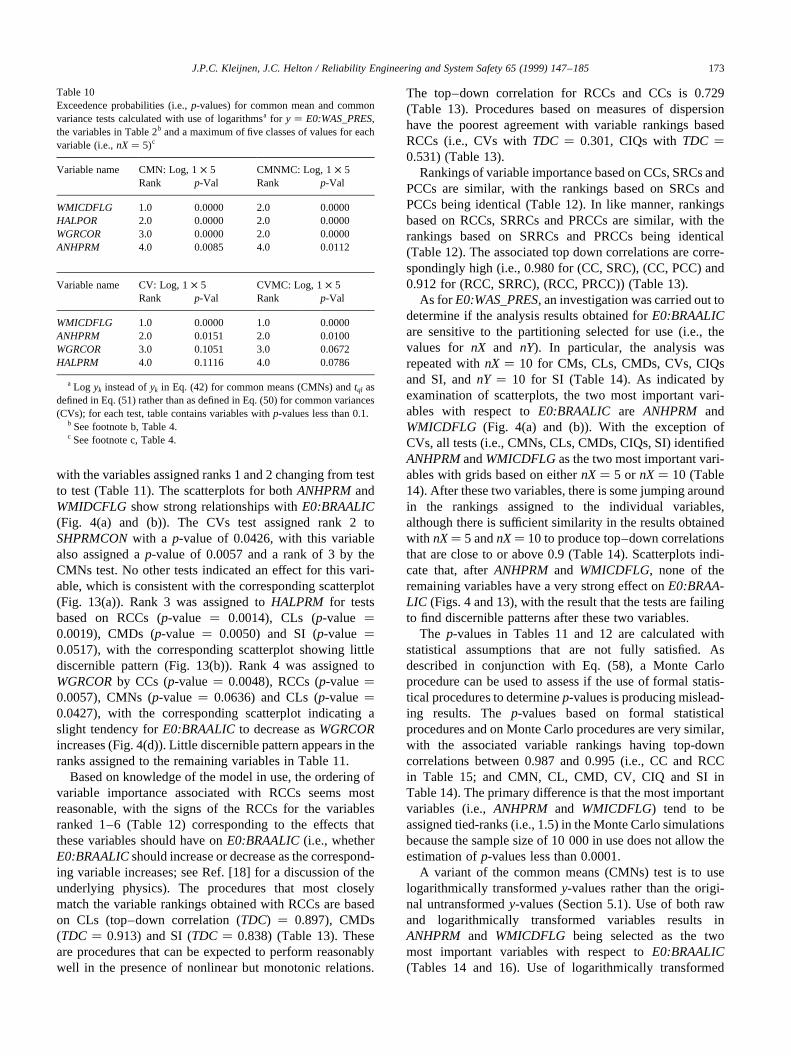
with the variables assigned ranks 1 and 2 changing from testto test (Table 11). The scatterplots for bothANHPRMandWMIDCFLG show strong relationships withE0:BRAALIC(Fig. 4(a) and (b)). The CVs test assigned rank 2 toSHPRMCONwith a p-value of 0.0426, with this variablealso assigned ap-value of 0.0057 and a rank of 3 by theCMNs test. No other tests indicated an effect for this vari-able, which is consistent with the corresponding scatterplot(Fig. 13(a)). Rank 3 was assigned toHALPRM for testsbased on RCCs (p-value � 0.0014), CLs (p-value �0.0019), CMDs (p-value � 0.0050) and SI (p-value �0.0517), with the corresponding scatterplot showing littlediscernible pattern (Fig. 13(b)). Rank 4 was assigned toWGRCORby CCs (p-value� 0.0048), RCCs (p-value�0.0057), CMNs (p-value� 0.0636) and CLs (p-value�0.0427), with the corresponding scatterplot indicating aslight tendency forE0:BRAALICto decrease asWGRCORincreases (Fig. 4(d)). Little discernible pattern appears in theranks assigned to the remaining variables in Table 11.
Based on knowledge of the model in use, the ordering ofvariable importance associated with RCCs seems mostreasonable, with the signs of the RCCs for the variablesranked 1–6 (Table 12) corresponding to the effects thatthese variables should have onE0:BRAALIC(i.e., whetherE0:BRAALICshould increase or decrease as the correspond-ing variable increases; see Ref. [18] for a discussion of theunderlying physics). The procedures that most closelymatch the variable rankings obtained with RCCs are basedon CLs (top–down correlation (TDC) � 0.897), CMDs(TDC � 0.913) and SI (TDC � 0.838) (Table 13). Theseare procedures that can be expected to perform reasonablywell in the presence of nonlinear but monotonic relations.
The top–down correlation for RCCs and CCs is 0.729(Table 13). Procedures based on measures of dispersionhave the poorest agreement with variable rankings basedRCCs (i.e., CVs withTDC � 0.301, CIQs withTDC �0.531) (Table 13).
Rankings of variable importance based on CCs, SRCs andPCCs are similar, with the rankings based on SRCs andPCCs being identical (Table 12). In like manner, rankingsbased on RCCs, SRRCs and PRCCs are similar, with therankings based on SRRCs and PRCCs being identical(Table 12). The associated top down correlations are corre-spondingly high (i.e., 0.980 for (CC, SRC), (CC, PCC) and0.912 for (RCC, SRRC), (RCC, PRCC)) (Table 13).
As for E0:WAS_PRES, an investigation was carried out todetermine if the analysis results obtained forE0:BRAALICare sensitive to the partitioning selected for use (i.e., thevalues for nX and nY). In particular, the analysis wasrepeated withnX � 10 for CMs, CLs, CMDs, CVs, CIQsand SI, andnY � 10 for SI (Table 14). As indicated byexamination of scatterplots, the two most important vari-ables with respect toE0:BRAALIC are ANHPRM andWMICDFLG (Fig. 4(a) and (b)). With the exception ofCVs, all tests (i.e., CMNs, CLs, CMDs, CIQs, SI) identifiedANHPRMandWMICDFLGas the two most important vari-ables with grids based on eithernX� 5 or nX� 10 (Table14). After these two variables, there is some jumping aroundin the rankings assigned to the individual variables,although there is sufficient similarity in the results obtainedwith nX� 5 andnX� 10 to produce top–down correlationsthat are close to or above 0.9 (Table 14). Scatterplots indi-cate that, afterANHPRM and WMICDFLG, none of theremaining variables have a very strong effect onE0:BRAA-LIC (Figs. 4 and 13), with the result that the tests are failingto find discernible patterns after these two variables.
The p-values in Tables 11 and 12 are calculated withstatistical assumptions that are not fully satisfied. Asdescribed in conjunction with Eq. (58), a Monte Carloprocedure can be used to assess if the use of formal statis-tical procedures to determinep-values is producing mislead-ing results. The p-values based on formal statisticalprocedures and on Monte Carlo procedures are very similar,with the associated variable rankings having top-downcorrelations between 0.987 and 0.995 (i.e., CC and RCCin Table 15; and CMN, CL, CMD, CV, CIQ and SI inTable 14). The primary difference is that the most importantvariables (i.e.,ANHPRM and WMICDFLG) tend to beassigned tied-ranks (i.e., 1.5) in the Monte Carlo simulationsbecause the sample size of 10 000 in use does not allow theestimation ofp-values less than 0.0001.
A variant of the common means (CMNs) test is to uselogarithmically transformedy-values rather than the origi-nal untransformedy-values (Section 5.1). Use of both rawand logarithmically transformed variables results inANHPRM and WMICDFLG being selected as the twomost important variables with respect toE0:BRAALIC(Tables 14 and 16). Use of logarithmically transformed
J.P.C. Kleijnen, J.C. Helton / Reliability Engineering and System Safety 65 (1999) 147–185 173
Table 10Exceedence probabilities (i.e.,p-values) for common mean and commonvariance tests calculated with use of logarithmsa for y � E0:WAS_PRES,the variables in Table 2b and a maximum of five classes of values for eachvariable (i.e.,nX� 5)c
Variable name CMN: Log, 1× 5 CMNMC: Log, 1× 5Rank p-Val Rank p-Val
WMICDFLG 1.0 0.0000 2.0 0.0000HALPOR 2.0 0.0000 2.0 0.0000WGRCOR 3.0 0.0000 2.0 0.0000ANHPRM 4.0 0.0085 4.0 0.0112
Variable name CV: Log, 1× 5 CVMC: Log, 1× 5Rank p-Val Rank p-Val
WMICDFLG 1.0 0.0000 1.0 0.0000ANHPRM 2.0 0.0151 2.0 0.0100WGRCOR 3.0 0.1051 3.0 0.0672HALPRM 4.0 0.1116 4.0 0.0786
a Log yk instead ofyk in Eq. (42) for common means (CMNs) andtql asdefined in Eq. (51) rather than as defined in Eq. (50) for common variances(CVs); for each test, table contains variables withp-values less than 0.1.
b See footnote b, Table 4.c See footnote c, Table 4.
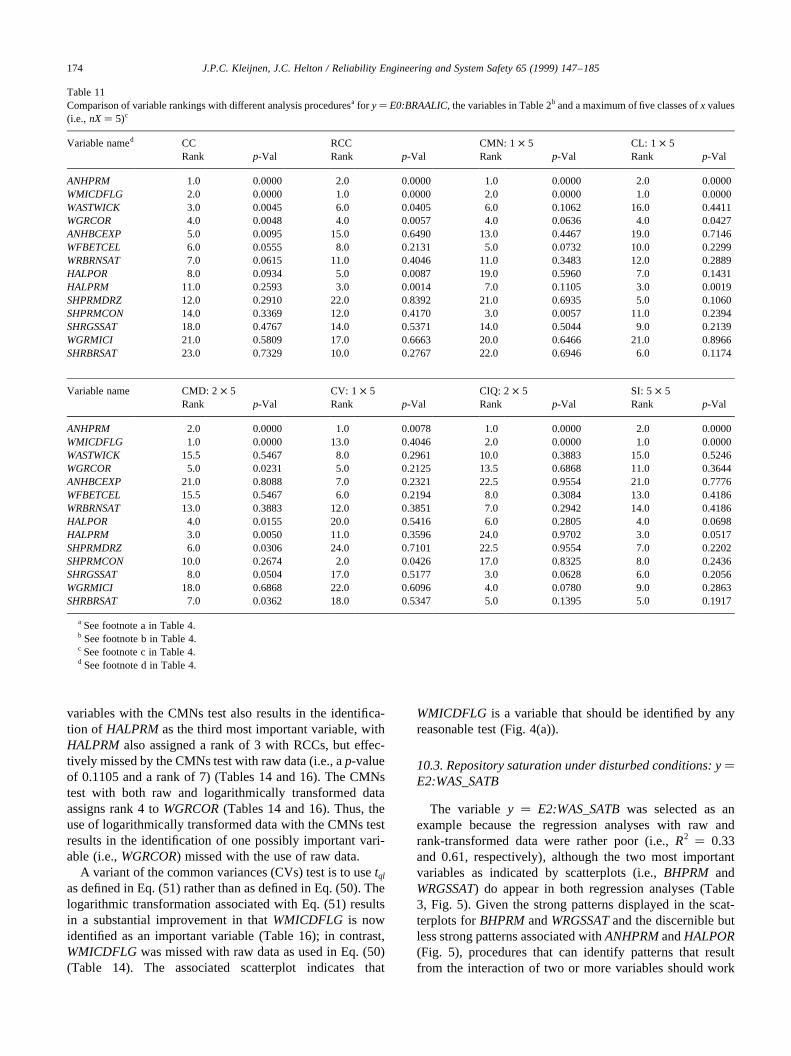
variables with the CMNs test also results in the identifica-tion of HALPRMas the third most important variable, withHALPRMalso assigned a rank of 3 with RCCs, but effec-tively missed by the CMNs test with raw data (i.e., ap-valueof 0.1105 and a rank of 7) (Tables 14 and 16). The CMNstest with both raw and logarithmically transformed dataassigns rank 4 toWGRCOR(Tables 14 and 16). Thus, theuse of logarithmically transformed data with the CMNs testresults in the identification of one possibly important vari-able (i.e.,WGRCOR) missed with the use of raw data.
A variant of the common variances (CVs) test is to usetql
as defined in Eq. (51) rather than as defined in Eq. (50). Thelogarithmic transformation associated with Eq. (51) resultsin a substantial improvement in thatWMICDFLG is nowidentified as an important variable (Table 16); in contrast,WMICDFLGwas missed with raw data as used in Eq. (50)(Table 14). The associated scatterplot indicates that
WMICDFLG is a variable that should be identified by anyreasonable test (Fig. 4(a)).
10.3. Repository saturation under disturbed conditions: y�E2:WAS_SATB
The variabley � E2:WAS_SATBwas selected as anexample because the regression analyses with raw andrank-transformed data were rather poor (i.e.,R2 � 0.33and 0.61, respectively), although the two most importantvariables as indicated by scatterplots (i.e.,BHPRM andWRGSSAT) do appear in both regression analyses (Table3, Fig. 5). Given the strong patterns displayed in the scat-terplots forBHPRMandWRGSSATand the discernible butless strong patterns associated withANHPRMandHALPOR(Fig. 5), procedures that can identify patterns that resultfrom the interaction of two or more variables should work
J.P.C. Kleijnen, J.C. Helton / Reliability Engineering and System Safety 65 (1999) 147–185174
Table 11Comparison of variable rankings with different analysis proceduresa for y� E0:BRAALIC, the variables in Table 2b and a maximum of five classes ofx values(i.e., nX� 5)c
Variable named CC RCC CMN: 1× 5 CL: 1 × 5Rank p-Val Rank p-Val Rank p-Val Rank p-Val
ANHPRM 1.0 0.0000 2.0 0.0000 1.0 0.0000 2.0 0.0000WMICDFLG 2.0 0.0000 1.0 0.0000 2.0 0.0000 1.0 0.0000WASTWICK 3.0 0.0045 6.0 0.0405 6.0 0.1062 16.0 0.4411WGRCOR 4.0 0.0048 4.0 0.0057 4.0 0.0636 4.0 0.0427ANHBCEXP 5.0 0.0095 15.0 0.6490 13.0 0.4467 19.0 0.7146WFBETCEL 6.0 0.0555 8.0 0.2131 5.0 0.0732 10.0 0.2299WRBRNSAT 7.0 0.0615 11.0 0.4046 11.0 0.3483 12.0 0.2889HALPOR 8.0 0.0934 5.0 0.0087 19.0 0.5960 7.0 0.1431HALPRM 11.0 0.2593 3.0 0.0014 7.0 0.1105 3.0 0.0019SHPRMDRZ 12.0 0.2910 22.0 0.8392 21.0 0.6935 5.0 0.1060SHPRMCON 14.0 0.3369 12.0 0.4170 3.0 0.0057 11.0 0.2394SHRGSSAT 18.0 0.4767 14.0 0.5371 14.0 0.5044 9.0 0.2139WGRMICI 21.0 0.5809 17.0 0.6663 20.0 0.6466 21.0 0.8966SHRBRSAT 23.0 0.7329 10.0 0.2767 22.0 0.6946 6.0 0.1174
Variable name CMD: 2× 5 CV: 1 × 5 CIQ: 2× 5 SI: 5× 5Rank p-Val Rank p-Val Rank p-Val Rank p-Val
ANHPRM 2.0 0.0000 1.0 0.0078 1.0 0.0000 2.0 0.0000WMICDFLG 1.0 0.0000 13.0 0.4046 2.0 0.0000 1.0 0.0000WASTWICK 15.5 0.5467 8.0 0.2961 10.0 0.3883 15.0 0.5246WGRCOR 5.0 0.0231 5.0 0.2125 13.5 0.6868 11.0 0.3644ANHBCEXP 21.0 0.8088 7.0 0.2321 22.5 0.9554 21.0 0.7776WFBETCEL 15.5 0.5467 6.0 0.2194 8.0 0.3084 13.0 0.4186WRBRNSAT 13.0 0.3883 12.0 0.3851 7.0 0.2942 14.0 0.4186HALPOR 4.0 0.0155 20.0 0.5416 6.0 0.2805 4.0 0.0698HALPRM 3.0 0.0050 11.0 0.3596 24.0 0.9702 3.0 0.0517SHPRMDRZ 6.0 0.0306 24.0 0.7101 22.5 0.9554 7.0 0.2202SHPRMCON 10.0 0.2674 2.0 0.0426 17.0 0.8325 8.0 0.2436SHRGSSAT 8.0 0.0504 17.0 0.5177 3.0 0.0628 6.0 0.2056WGRMICI 18.0 0.6868 22.0 0.6096 4.0 0.0780 9.0 0.2863SHRBRSAT 7.0 0.0362 18.0 0.5347 5.0 0.1395 5.0 0.1917
a See footnote a in Table 4.b See footnote b in Table 4.c See footnote c in Table 4.d See footnote d in Table 4.
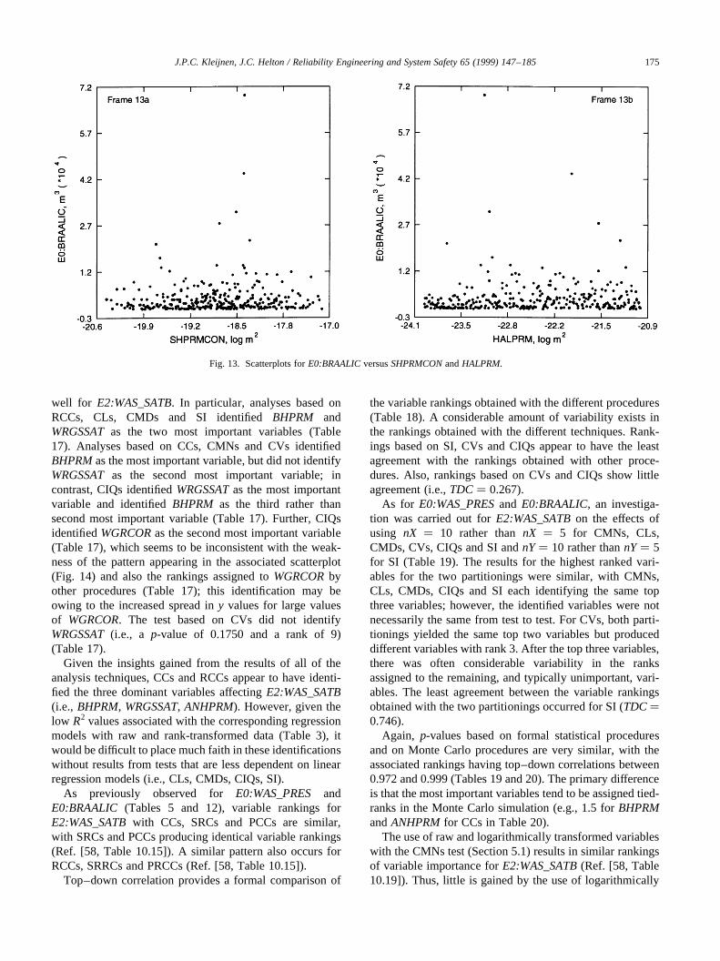
well for E2:WAS_SATB. In particular, analyses based onRCCs, CLs, CMDs and SI identifiedBHPRM andWRGSSATas the two most important variables (Table17). Analyses based on CCs, CMNs and CVs identifiedBHPRMas the most important variable, but did not identifyWRGSSATas the second most important variable; incontrast, CIQs identifiedWRGSSATas the most importantvariable and identifiedBHPRM as the third rather thansecond most important variable (Table 17). Further, CIQsidentifiedWGRCORas the second most important variable(Table 17), which seems to be inconsistent with the weak-ness of the pattern appearing in the associated scatterplot(Fig. 14) and also the rankings assigned toWGRCORbyother procedures (Table 17); this identification may beowing to the increased spread iny values for large valuesof WGRCOR. The test based on CVs did not identifyWRGSSAT(i.e., a p-value of 0.1750 and a rank of 9)(Table 17).
Given the insights gained from the results of all of theanalysis techniques, CCs and RCCs appear to have identi-fied the three dominant variables affectingE2:WAS_SATB(i.e., BHPRM, WRGSSAT, ANHPRM). However, given thelow R2 values associated with the corresponding regressionmodels with raw and rank-transformed data (Table 3), itwould be difficult to place much faith in these identificationswithout results from tests that are less dependent on linearregression models (i.e., CLs, CMDs, CIQs, SI).
As previously observed for E0:WAS_PRES andE0:BRAALIC (Tables 5 and 12), variable rankings forE2:WAS_SATBwith CCs, SRCs and PCCs are similar,with SRCs and PCCs producing identical variable rankings(Ref. [58, Table 10.15]). A similar pattern also occurs forRCCs, SRRCs and PRCCs (Ref. [58, Table 10.15]).
Top–down correlation provides a formal comparison of
the variable rankings obtained with the different procedures(Table 18). A considerable amount of variability exists inthe rankings obtained with the different techniques. Rank-ings based on SI, CVs and CIQs appear to have the leastagreement with the rankings obtained with other proce-dures. Also, rankings based on CVs and CIQs show littleagreement (i.e.,TDC� 0.267).
As for E0:WAS_PRESand E0:BRAALIC, an investiga-tion was carried out forE2:WAS_SATBon the effects ofusing nX � 10 rather thannX � 5 for CMNs, CLs,CMDs, CVs, CIQs and SI andnY� 10 rather thannY� 5for SI (Table 19). The results for the highest ranked vari-ables for the two partitionings were similar, with CMNs,CLs, CMDs, CIQs and SI each identifying the same topthree variables; however, the identified variables were notnecessarily the same from test to test. For CVs, both parti-tionings yielded the same top two variables but produceddifferent variables with rank 3. After the top three variables,there was often considerable variability in the ranksassigned to the remaining, and typically unimportant, vari-ables. The least agreement between the variable rankingsobtained with the two partitionings occurred for SI (TDC�0.746).
Again, p-values based on formal statistical proceduresand on Monte Carlo procedures are very similar, with theassociated rankings having top–down correlations between0.972 and 0.999 (Tables 19 and 20). The primary differenceis that the most important variables tend to be assigned tied-ranks in the Monte Carlo simulation (e.g., 1.5 forBHPRMandANHPRMfor CCs in Table 20).
The use of raw and logarithmically transformed variableswith the CMNs test (Section 5.1) results in similar rankingsof variable importance forE2:WAS_SATB(Ref. [58, Table10.19]). Thus, little is gained by the use of logarithmically
J.P.C. Kleijnen, J.C. Helton / Reliability Engineering and System Safety 65 (1999) 147–185 175
Fig. 13. Scatterplots forE0:BRAALICversusSHPRMCONandHALPRM.
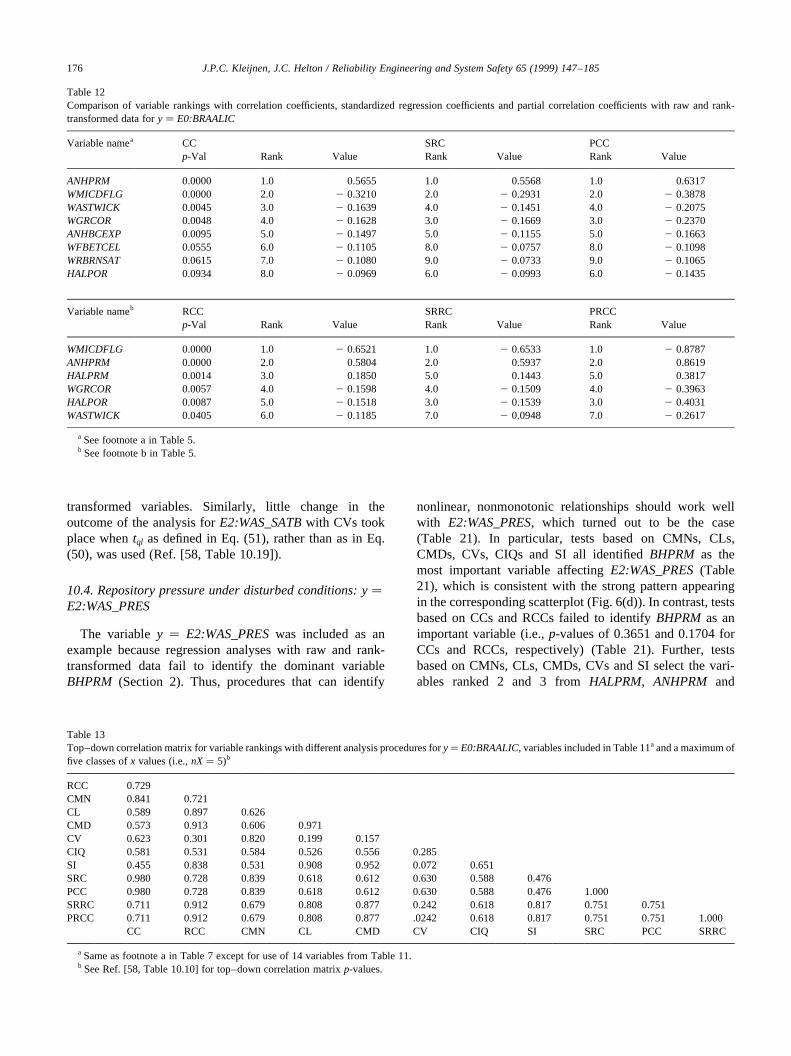
transformed variables. Similarly, little change in theoutcome of the analysis forE2:WAS_SATBwith CVs tookplace whentql as defined in Eq. (51), rather than as in Eq.(50), was used (Ref. [58, Table 10.19]).
10.4. Repository pressure under disturbed conditions: y�E2:WAS_PRES
The variabley � E2:WAS_PRESwas included as anexample because regression analyses with raw and rank-transformed data fail to identify the dominant variableBHPRM (Section 2). Thus, procedures that can identify
nonlinear, nonmonotonic relationships should work wellwith E2:WAS_PRES, which turned out to be the case(Table 21). In particular, tests based on CMNs, CLs,CMDs, CVs, CIQs and SI all identifiedBHPRM as themost important variable affectingE2:WAS_PRES(Table21), which is consistent with the strong pattern appearingin the corresponding scatterplot (Fig. 6(d)). In contrast, testsbased on CCs and RCCs failed to identifyBHPRM as animportant variable (i.e.,p-values of 0.3651 and 0.1704 forCCs and RCCs, respectively) (Table 21). Further, testsbased on CMNs, CLs, CMDs, CVs and SI select the vari-ables ranked 2 and 3 fromHALPRM, ANHPRM and
J.P.C. Kleijnen, J.C. Helton / Reliability Engineering and System Safety 65 (1999) 147–185176
Table 12Comparison of variable rankings with correlation coefficients, standardized regression coefficients and partial correlation coefficients with rawand rank-transformed data fory � E0:BRAALIC
Variable namea CC SRC PCCp-Val Rank Value Rank Value Rank Value
ANHPRM 0.0000 1.0 0.5655 1.0 0.5568 1.0 0.6317WMICDFLG 0.0000 2.0 2 0.3210 2.0 2 0.2931 2.0 2 0.3878WASTWICK 0.0045 3.0 2 0.1639 4.0 2 0.1451 4.0 2 0.2075WGRCOR 0.0048 4.0 2 0.1628 3.0 2 0.1669 3.0 2 0.2370ANHBCEXP 0.0095 5.0 2 0.1497 5.0 2 0.1155 5.0 2 0.1663WFBETCEL 0.0555 6.0 2 0.1105 8.0 2 0.0757 8.0 2 0.1098WRBRNSAT 0.0615 7.0 2 0.1080 9.0 2 0.0733 9.0 2 0.1065HALPOR 0.0934 8.0 2 0.0969 6.0 2 0.0993 6.0 2 0.1435
Variable nameb RCC SRRC PRCCp-Val Rank Value Rank Value Rank Value
WMICDFLG 0.0000 1.0 2 0.6521 1.0 2 0.6533 1.0 2 0.8787ANHPRM 0.0000 2.0 0.5804 2.0 0.5937 2.0 0.8619HALPRM 0.0014 3.0 0.1850 5.0 0.1443 5.0 0.3817WGRCOR 0.0057 4.0 2 0.1598 4.0 2 0.1509 4.0 2 0.3963HALPOR 0.0087 5.0 2 0.1518 3.0 2 0.1539 3.0 2 0.4031WASTWICK 0.0405 6.0 2 0.1185 7.0 2 0.0948 7.0 2 0.2617
a See footnote a in Table 5.b See footnote b in Table 5.
Table 13Top–down correlation matrix for variable rankings with different analysis procedures fory� E0:BRAALIC, variables included in Table 11a and a maximum offive classes ofx values (i.e.,nX� 5)b
RCC 0.729CMN 0.841 0.721CL 0.589 0.897 0.626CMD 0.573 0.913 0.606 0.971CV 0.623 0.301 0.820 0.199 0.157CIQ 0.581 0.531 0.584 0.526 0.556 0.285SI 0.455 0.838 0.531 0.908 0.952 0.072 0.651SRC 0.980 0.728 0.839 0.618 0.612 0.630 0.588 0.476PCC 0.980 0.728 0.839 0.618 0.612 0.630 0.588 0.476 1.000SRRC 0.711 0.912 0.679 0.808 0.877 0.242 0.618 0.817 0.751 0.751PRCC 0.711 0.912 0.679 0.808 0.877 .0242 0.618 0.817 0.751 0.751 1.000
CC RCC CMN CL CMD CV CIQ SI SRC PCC SRRC
a Same as footnote a in Table 7 except for use of 14 variables from Table 11.b See Ref. [58, Table 10.10] for top–down correlation matrixp-values.
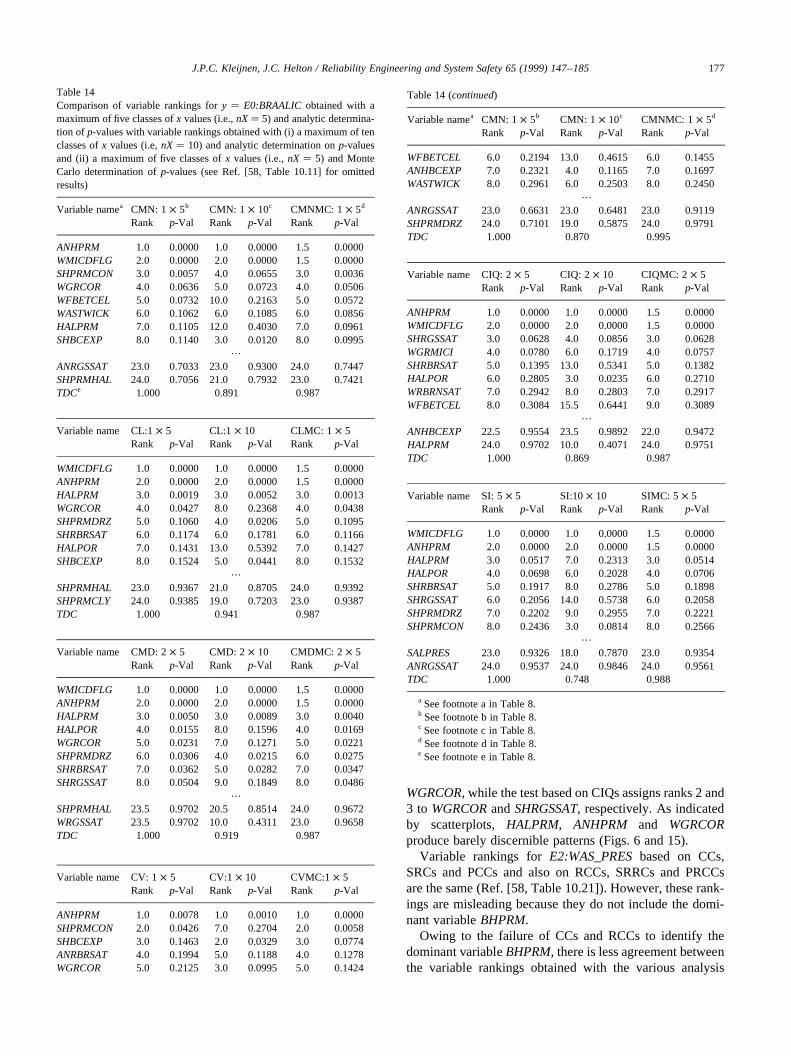
WGRCOR, while the test based on CIQs assigns ranks 2 and3 to WGRCORandSHRGSSAT, respectively. As indicatedby scatterplots, HALPRM, ANHPRM and WGRCORproduce barely discernible patterns (Figs. 6 and 15).
Variable rankings forE2:WAS_PRESbased on CCs,SRCs and PCCs and also on RCCs, SRRCs and PRCCsare the same (Ref. [58, Table 10.21]). However, these rank-ings are misleading because they do not include the domi-nant variableBHPRM.
Owing to the failure of CCs and RCCs to identify thedominant variableBHPRM, there is less agreement betweenthe variable rankings obtained with the various analysis
J.P.C. Kleijnen, J.C. Helton / Reliability Engineering and System Safety 65 (1999) 147–185 177
Table 14Comparison of variable rankings fory � E0:BRAALICobtained with amaximum of five classes ofx values (i.e.,nX� 5) and analytic determina-tion of p-values with variable rankings obtained with (i) a maximum of tenclasses ofx values (i.e,nX� 10) and analytic determination onp-valuesand (ii) a maximum of five classes ofx values (i.e.,nX � 5) and MonteCarlo determination ofp-values (see Ref. [58, Table 10.11] for omittedresults)
Variable namea CMN: 1 × 5b CMN: 1 × 10c CMNMC: 1 × 5d
Rank p-Val Rank p-Val Rank p-Val
ANHPRM 1.0 0.0000 1.0 0.0000 1.5 0.0000WMICDFLG 2.0 0.0000 2.0 0.0000 1.5 0.0000SHPRMCON 3.0 0.0057 4.0 0.0655 3.0 0.0036WGRCOR 4.0 0.0636 5.0 0.0723 4.0 0.0506WFBETCEL 5.0 0.0732 10.0 0.2163 5.0 0.0572WASTWICK 6.0 0.1062 6.0 0.1085 6.0 0.0856HALPRM 7.0 0.1105 12.0 0.4030 7.0 0.0961SHBCEXP 8.0 0.1140 3.0 0.0120 8.0 0.0995
…
ANRGSSAT 23.0 0.7033 23.0 0.9300 24.0 0.7447SHPRMHAL 24.0 0.7056 21.0 0.7932 23.0 0.7421TDCe 1.000 0.891 0.987
Variable name CL:1× 5 CL:1 × 10 CLMC: 1× 5Rank p-Val Rank p-Val Rank p-Val
WMICDFLG 1.0 0.0000 1.0 0.0000 1.5 0.0000ANHPRM 2.0 0.0000 2.0 0.0000 1.5 0.0000HALPRM 3.0 0.0019 3.0 0.0052 3.0 0.0013WGRCOR 4.0 0.0427 8.0 0.2368 4.0 0.0438SHPRMDRZ 5.0 0.1060 4.0 0.0206 5.0 0.1095SHRBRSAT 6.0 0.1174 6.0 0.1781 6.0 0.1166HALPOR 7.0 0.1431 13.0 0.5392 7.0 0.1427SHBCEXP 8.0 0.1524 5.0 0.0441 8.0 0.1532
…
SHPRMHAL 23.0 0.9367 21.0 0.8705 24.0 0.9392SHPRMCLY 24.0 0.9385 19.0 0.7203 23.0 0.9387TDC 1.000 0.941 0.987
Variable name CMD: 2× 5 CMD: 2 × 10 CMDMC: 2× 5Rank p-Val Rank p-Val Rank p-Val
WMICDFLG 1.0 0.0000 1.0 0.0000 1.5 0.0000ANHPRM 2.0 0.0000 2.0 0.0000 1.5 0.0000HALPRM 3.0 0.0050 3.0 0.0089 3.0 0.0040HALPOR 4.0 0.0155 8.0 0.1596 4.0 0.0169WGRCOR 5.0 0.0231 7.0 0.1271 5.0 0.0221SHPRMDRZ 6.0 0.0306 4.0 0.0215 6.0 0.0275SHRBRSAT 7.0 0.0362 5.0 0.0282 7.0 0.0347SHRGSSAT 8.0 0.0504 9.0 0.1849 8.0 0.0486
…
SHPRMHAL 23.5 0.9702 20.5 0.8514 24.0 0.9672WRGSSAT 23.5 0.9702 10.0 0.4311 23.0 0.9658TDC 1.000 0.919 0.987
Variable name CV: 1× 5 CV:1 × 10 CVMC:1× 5Rank p-Val Rank p-Val Rank p-Val
ANHPRM 1.0 0.0078 1.0 0.0010 1.0 0.0000SHPRMCON 2.0 0.0426 7.0 0.2704 2.0 0.0058SHBCEXP 3.0 0.1463 2.0 0.0329 3.0 0.0774ANRBRSAT 4.0 0.1994 5.0 0.1188 4.0 0.1278WGRCOR 5.0 0.2125 3.0 0.0995 5.0 0.1424
Table 14 (continued)
Variable namea CMN: 1 × 5b CMN: 1 × 10c CMNMC: 1 × 5d
Rank p-Val Rank p-Val Rank p-Val
WFBETCEL 6.0 0.2194 13.0 0.4615 6.0 0.1455ANHBCEXP 7.0 0.2321 4.0 0.1165 7.0 0.1697WASTWICK 8.0 0.2961 6.0 0.2503 8.0 0.2450
…
ANRGSSAT 23.0 0.6631 23.0 0.6481 23.0 0.9119SHPRMDRZ 24.0 0.7101 19.0 0.5875 24.0 0.9791TDC 1.000 0.870 0.995
Variable name CIQ: 2× 5 CIQ: 2× 10 CIQMC: 2× 5Rank p-Val Rank p-Val Rank p-Val
ANHPRM 1.0 0.0000 1.0 0.0000 1.5 0.0000WMICDFLG 2.0 0.0000 2.0 0.0000 1.5 0.0000SHRGSSAT 3.0 0.0628 4.0 0.0856 3.0 0.0628WGRMICI 4.0 0.0780 6.0 0.1719 4.0 0.0757SHRBRSAT 5.0 0.1395 13.0 0.5341 5.0 0.1382HALPOR 6.0 0.2805 3.0 0.0235 6.0 0.2710WRBRNSAT 7.0 0.2942 8.0 0.2803 7.0 0.2917WFBETCEL 8.0 0.3084 15.5 0.6441 9.0 0.3089
…
ANHBCEXP 22.5 0.9554 23.5 0.9892 22.0 0.9472HALPRM 24.0 0.9702 10.0 0.4071 24.0 0.9751TDC 1.000 0.869 0.987
Variable name SI: 5× 5 SI:10× 10 SIMC: 5× 5Rank p-Val Rank p-Val Rank p-Val
WMICDFLG 1.0 0.0000 1.0 0.0000 1.5 0.0000ANHPRM 2.0 0.0000 2.0 0.0000 1.5 0.0000HALPRM 3.0 0.0517 7.0 0.2313 3.0 0.0514HALPOR 4.0 0.0698 6.0 0.2028 4.0 0.0706SHRBRSAT 5.0 0.1917 8.0 0.2786 5.0 0.1898SHRGSSAT 6.0 0.2056 14.0 0.5738 6.0 0.2058SHPRMDRZ 7.0 0.2202 9.0 0.2955 7.0 0.2221SHPRMCON 8.0 0.2436 3.0 0.0814 8.0 0.2566
…
SALPRES 23.0 0.9326 18.0 0.7870 23.0 0.9354ANRGSSAT 24.0 0.9537 24.0 0.9846 24.0 0.9561TDC 1.000 0.748 0.988
a See footnote a in Table 8.b See footnote b in Table 8.c See footnote c in Table 8.d See footnote d in Table 8.e See footnote e in Table 8.
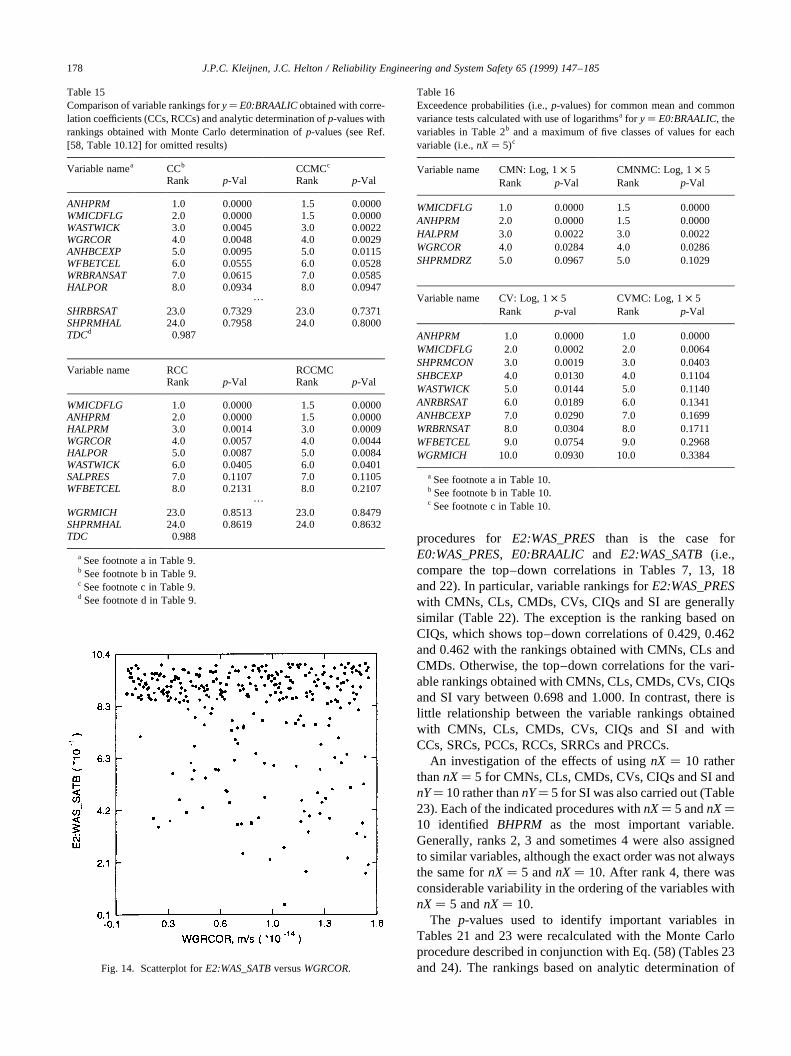
procedures for E2:WAS_PRESthan is the case forE0:WAS_PRES, E0:BRAALIC and E2:WAS_SATB(i.e.,compare the top–down correlations in Tables 7, 13, 18and 22). In particular, variable rankings forE2:WAS_PRESwith CMNs, CLs, CMDs, CVs, CIQs and SI are generallysimilar (Table 22). The exception is the ranking based onCIQs, which shows top–down correlations of 0.429, 0.462and 0.462 with the rankings obtained with CMNs, CLs andCMDs. Otherwise, the top–down correlations for the vari-able rankings obtained with CMNs, CLs, CMDs, CVs, CIQsand SI vary between 0.698 and 1.000. In contrast, there islittle relationship between the variable rankings obtainedwith CMNs, CLs, CMDs, CVs, CIQs and SI and withCCs, SRCs, PCCs, RCCs, SRRCs and PRCCs.
An investigation of the effects of usingnX � 10 ratherthannX� 5 for CMNs, CLs, CMDs, CVs, CIQs and SI andnY� 10 rather thannY� 5 for SI was also carried out (Table23). Each of the indicated procedures withnX� 5 andnX�10 identified BHPRM as the most important variable.Generally, ranks 2, 3 and sometimes 4 were also assignedto similar variables, although the exact order was not alwaysthe same fornX� 5 andnX� 10. After rank 4, there wasconsiderable variability in the ordering of the variables withnX� 5 andnX� 10.
The p-values used to identify important variables inTables 21 and 23 were recalculated with the Monte Carloprocedure described in conjunction with Eq. (58) (Tables 23and 24). The rankings based on analytic determination of
J.P.C. Kleijnen, J.C. Helton / Reliability Engineering and System Safety 65 (1999) 147–185178
Table 15Comparison of variable rankings fory� E0:BRAALICobtained with corre-lation coefficients (CCs, RCCs) and analytic determination ofp-values withrankings obtained with Monte Carlo determination ofp-values (see Ref.[58, Table 10.12] for omitted results)
Variable namea CCb CCMCc
Rank p-Val Rank p-Val
ANHPRM 1.0 0.0000 1.5 0.0000WMICDFLG 2.0 0.0000 1.5 0.0000WASTWICK 3.0 0.0045 3.0 0.0022WGRCOR 4.0 0.0048 4.0 0.0029ANHBCEXP 5.0 0.0095 5.0 0.0115WFBETCEL 6.0 0.0555 6.0 0.0528WRBRANSAT 7.0 0.0615 7.0 0.0585HALPOR 8.0 0.0934 8.0 0.0947
…SHRBRSAT 23.0 0.7329 23.0 0.7371SHPRMHAL 24.0 0.7958 24.0 0.8000TDCd 0.987
Variable name RCC RCCMCRank p-Val Rank p-Val
WMICDFLG 1.0 0.0000 1.5 0.0000ANHPRM 2.0 0.0000 1.5 0.0000HALPRM 3.0 0.0014 3.0 0.0009WGRCOR 4.0 0.0057 4.0 0.0044HALPOR 5.0 0.0087 5.0 0.0084WASTWICK 6.0 0.0405 6.0 0.0401SALPRES 7.0 0.1107 7.0 0.1105WFBETCEL 8.0 0.2131 8.0 0.2107
…WGRMICH 23.0 0.8513 23.0 0.8479SHPRMHAL 24.0 0.8619 24.0 0.8632TDC 0.988
a See footnote a in Table 9.b See footnote b in Table 9.c See footnote c in Table 9.d See footnote d in Table 9.
Table 16Exceedence probabilities (i.e.,p-values) for common mean and commonvariance tests calculated with use of logarithmsa for y� E0:BRAALIC, thevariables in Table 2b and a maximum of five classes of values for eachvariable (i.e.,nX� 5)c
Variable name CMN: Log, 1× 5 CMNMC: Log, 1× 5Rank p-Val Rank p-Val
WMICDFLG 1.0 0.0000 1.5 0.0000ANHPRM 2.0 0.0000 1.5 0.0000HALPRM 3.0 0.0022 3.0 0.0022WGRCOR 4.0 0.0284 4.0 0.0286SHPRMDRZ 5.0 0.0967 5.0 0.1029
Variable name CV: Log, 1× 5 CVMC: Log, 1× 5Rank p-val Rank p-Val
ANHPRM 1.0 0.0000 1.0 0.0000WMICDFLG 2.0 0.0002 2.0 0.0064SHPRMCON 3.0 0.0019 3.0 0.0403SHBCEXP 4.0 0.0130 4.0 0.1104WASTWICK 5.0 0.0144 5.0 0.1140ANRBRSAT 6.0 0.0189 6.0 0.1341ANHBCEXP 7.0 0.0290 7.0 0.1699WRBRNSAT 8.0 0.0304 8.0 0.1711WFBETCEL 9.0 0.0754 9.0 0.2968WGRMICH 10.0 0.0930 10.0 0.3384
a See footnote a in Table 10.b See footnote b in Table 10.c See footnote c in Table 10.
Fig. 14. Scatterplot forE2:WAS_SATBversusWGRCOR.
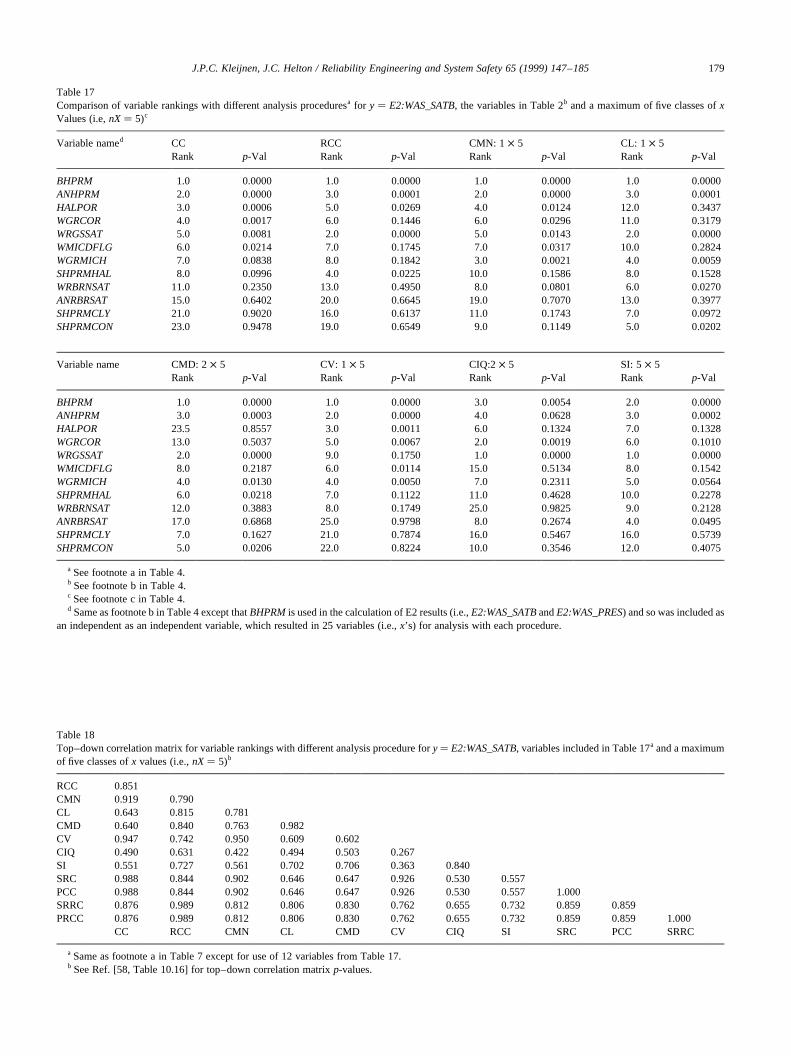
J.P.C. Kleijnen, J.C. Helton / Reliability Engineering and System Safety 65 (1999) 147–185 179
Table 17Comparison of variable rankings with different analysis proceduresa for y � E2:WAS_SATB, the variables in Table 2b and a maximum of five classes ofxValues (i.e,nX� 5)c
Variable named CC RCC CMN: 1× 5 CL: 1 × 5Rank p-Val Rank p-Val Rank p-Val Rank p-Val
BHPRM 1.0 0.0000 1.0 0.0000 1.0 0.0000 1.0 0.0000ANHPRM 2.0 0.0000 3.0 0.0001 2.0 0.0000 3.0 0.0001HALPOR 3.0 0.0006 5.0 0.0269 4.0 0.0124 12.0 0.3437WGRCOR 4.0 0.0017 6.0 0.1446 6.0 0.0296 11.0 0.3179WRGSSAT 5.0 0.0081 2.0 0.0000 5.0 0.0143 2.0 0.0000WMICDFLG 6.0 0.0214 7.0 0.1745 7.0 0.0317 10.0 0.2824WGRMICH 7.0 0.0838 8.0 0.1842 3.0 0.0021 4.0 0.0059SHPRMHAL 8.0 0.0996 4.0 0.0225 10.0 0.1586 8.0 0.1528WRBRNSAT 11.0 0.2350 13.0 0.4950 8.0 0.0801 6.0 0.0270ANRBRSAT 15.0 0.6402 20.0 0.6645 19.0 0.7070 13.0 0.3977SHPRMCLY 21.0 0.9020 16.0 0.6137 11.0 0.1743 7.0 0.0972SHPRMCON 23.0 0.9478 19.0 0.6549 9.0 0.1149 5.0 0.0202
Variable name CMD: 2× 5 CV: 1 × 5 CIQ:2× 5 SI: 5× 5Rank p-Val Rank p-Val Rank p-Val Rank p-Val
BHPRM 1.0 0.0000 1.0 0.0000 3.0 0.0054 2.0 0.0000ANHPRM 3.0 0.0003 2.0 0.0000 4.0 0.0628 3.0 0.0002HALPOR 23.5 0.8557 3.0 0.0011 6.0 0.1324 7.0 0.1328WGRCOR 13.0 0.5037 5.0 0.0067 2.0 0.0019 6.0 0.1010WRGSSAT 2.0 0.0000 9.0 0.1750 1.0 0.0000 1.0 0.0000WMICDFLG 8.0 0.2187 6.0 0.0114 15.0 0.5134 8.0 0.1542WGRMICH 4.0 0.0130 4.0 0.0050 7.0 0.2311 5.0 0.0564SHPRMHAL 6.0 0.0218 7.0 0.1122 11.0 0.4628 10.0 0.2278WRBRNSAT 12.0 0.3883 8.0 0.1749 25.0 0.9825 9.0 0.2128ANRBRSAT 17.0 0.6868 25.0 0.9798 8.0 0.2674 4.0 0.0495SHPRMCLY 7.0 0.1627 21.0 0.7874 16.0 0.5467 16.0 0.5739SHPRMCON 5.0 0.0206 22.0 0.8224 10.0 0.3546 12.0 0.4075
a See footnote a in Table 4.b See footnote b in Table 4.c See footnote c in Table 4.d Same as footnote b in Table 4 except thatBHPRMis used in the calculation of E2 results (i.e.,E2:WAS_SATBandE2:WAS_PRES) and so was included as
an independent as an independent variable, which resulted in 25 variables (i.e.,x’s) for analysis with each procedure.
Table 18Top–down correlation matrix for variable rankings with different analysis procedure fory� E2:WAS_SATB, variables included in Table 17a and a maximumof five classes ofx values (i.e.,nX� 5)b
RCC 0.851CMN 0.919 0.790CL 0.643 0.815 0.781CMD 0.640 0.840 0.763 0.982CV 0.947 0.742 0.950 0.609 0.602CIQ 0.490 0.631 0.422 0.494 0.503 0.267SI 0.551 0.727 0.561 0.702 0.706 0.363 0.840SRC 0.988 0.844 0.902 0.646 0.647 0.926 0.530 0.557PCC 0.988 0.844 0.902 0.646 0.647 0.926 0.530 0.557 1.000SRRC 0.876 0.989 0.812 0.806 0.830 0.762 0.655 0.732 0.859 0.859PRCC 0.876 0.989 0.812 0.806 0.830 0.762 0.655 0.732 0.859 0.859 1.000
CC RCC CMN CL CMD CV CIQ SI SRC PCC SRRC
a Same as footnote a in Table 7 except for use of 12 variables from Table 17.b See Ref. [58, Table 10.16] for top–down correlation matrixp-values.
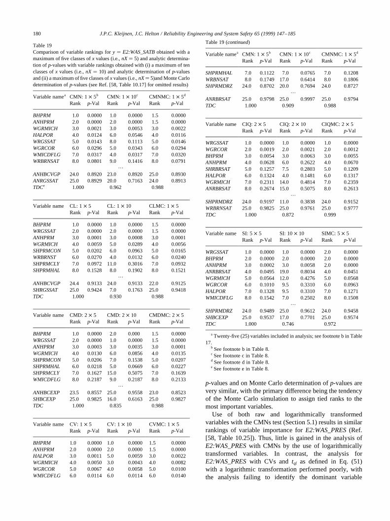
p-values and on Monte Carlo determination ofp-values arevery similar, with the primary difference being the tendencyof the Monte Carlo simulation to assign tied ranks to themost important variables.
Use of both raw and logarithmically transformedvariables with the CMNs test (Section 5.1) results in similarrankings of variable importance forE2:WAS_PRES(Ref.[58, Table 10.25]). Thus, little is gained in the analysis ofE2:WAS_PRESwith CMNs by the use of logarithmicallytransformed variables. In contrast, the analysis forE2:WAS_PRESwith CVs and tql as defined in Eq. (51)with a logarithmic transformation performed poorly, withthe analysis failing to identify the dominant variable
J.P.C. Kleijnen, J.C. Helton / Reliability Engineering and System Safety 65 (1999) 147–185180
Table 19Comparison of variable rankings fory � E2:WAS_SATBobtained with amaximum of five classes ofx values (i.e.,nX� 5) and analytic determina-tion of p-values with variable rankings obtained with (i) a maximum of tenclasses ofx values (i.e.,nX� 10) and analytic determination ofp-valuesand (ii) a maximum of five classes ofx values (i.e.,nX� 5)and Monte Carlodetermination ofp-values (see Ref. [58, Table 10.17] for omitted results)
Variable namea CMN: 1 × 5b CMN: 1 × 10c CMNMC: 1 × 5d
Rank p-Val Rank p-Val Rank p-Val
BHPRM 1.0 0.0000 1.0 0.0000 1.5 0.0000ANHPRM 2.0 0.0000 2.0 0.0000 1.5 0.0000WGRMICH 3.0 0.0021 3.0 0.0053 3.0 0.0022HALPOR 4.0 0.0124 6.0 0.0546 4.0 0.0116WRGSSAT 5.0 0.0143 8.0 0.1113 5.0 0.0146WGRCOR 6.0 0.0296 5.0 0.0343 6.0 0.0294WMICDFLG 7.0 0.0317 4.0 0.0317 7.0 0.0320WRBRNSAT 8.0 0.0801 9.0 0.1416 8.0 0.0791
…
ANHBCVGP 24.0 0.8920 23.0 0.8920 25.0 0.8930ANRGSSAT 25.0 0.8929 20.0 0.7163 24.0 0.8913TDCe 1.000 0.962 0.988
Variable name CL: 1× 5 CL: 1 × 10 CLMC: 1× 5Rank p-Val Rank p-Val Rank p-Val
BHPRM 1.0 0.0000 1.0 0.0000 1.5 0.0000WRGSSAT 2.0 0.0000 2.0 0.0000 1.5 0.0000ANHPRM 3.0 0.0001 3.0 0.0008 3.0 0.0001WGRMICH 4.0 0.0059 5.0 0.0289 4.0 0.0056SHPRMCON 5.0 0.0202 6.0 0.0963 5.0 0.0165WRBRNST 6.0 0.0270 4.0 0.0132 6.0 0.0240SHPRMCLY 7.0 0.0972 11.0 0.3016 7.0 0.0932SHPRMHAL 8.0 0.1528 8.0 0.1902 8.0 0.1521
…
ANHBCVGP 24.4 0.9133 24.0 0.9133 22.0 0.9125SHRGSSAT 25.0 0.9424 7.0 0.1763 25.0 0.9418TDC 1.000 0.930 0.988
Variable name CMD: 2× 5 CMD: 2 × 10 CMDMC: 2× 5Rank p-Val Rank p-Val Rank p-Val
BHPRM 1.0 0.0000 2.0 0.000 1.5 0.0000WRGSSAT 2.0 0.0000 1.0 0.0000 1.5 0.0000ANHPRM 3.0 0.0003 3.0 0.0035 3.0 0.0001WGRMICH 4.0 0.0130 6.0 0.0856 4.0 0.0135SHPRMCON 5.0 0.0206 7.0 0.1538 5.0 0.0207SHPRMHAL 6.0 0.0218 5.0 0.0669 6.0 0.0227SHPRMCLY 7.0 0.1627 15.0 0.5075 7.0 0.1639WMICDFLG 8.0 0.2187 9.0 0.2187 8.0 0.2133
…
ANHBCEXP 23.5 0.8557 25.0 0.9558 23.0 0.8523SHBCEXP 25.0 0.9825 16.0 0.6163 25.0 0.9827TDC 1.000 0.835 0.988
Variable name CV: 1× 5 CV: 1 × 10 CVMC: 1× 5Rank p-Val Rank p-Val Rank p-Val
BHPRM 1.0 0.0000 1.0 0.0000 1.5 0.0000ANHPRM 2.0 0.0000 2.0 0.0000 1.5 0.0000HALPOR 3.0 0.0011 5.0 0.0059 3.0 0.0022WGRMICH 4.0 0.0050 3.0 0.0043 4.0 0.0082WGRCOR 5.0 0.0067 4.0 0.0058 5.0 0.0100WMICDFLG 6.0 0.0114 6.0 0.0114 6.0 0.0140
Table 19 (continued)
Variable namea CMN: 1 × 5b CMN: 1 × 10c CMNMC: 1 × 5d
Rank p-Val Rank p-Val Rank p-Val
SHPRMHAL 7.0 0.1122 7.0 0.0765 7.0 0.1208WRBNSAT 8.0 0.1749 17.0 0.6414 8.0 0.1806SHPRMDRZ 24.0 0.8702 20.0 0.7694 24.0 0.8727
…
ANRBRSAT 25.0 0.9798 25.0 0.9997 25.0 0.9794TDC 1.000 0.909 0.988
Variable name CIQ: 2× 5 CIQ: 2× 10 CIQMC: 2× 5Rank p-Val Rank p-Val Rank p-Val
WRGSSAT 1.0 0.0000 1.0 0.0000 1.0 0.0000WGRCOR 2.0 0.0019 2.0 0.0021 2.0 0.0012BHPRM 3.0 0.0054 3.0 0.0063 3.0 0.0055ANHPRM 4.0 0.0628 6.0 0.2622 4.0 0.0670SHRBRSAT 5.0 0.1257 7.5 0.2803 5.0 0.1209HALPOR 6.0 0.1324 4.0 0.1481 6.0 0.1317WGRMICH 7.0 0.2311 14.0 0.4814 7.0 0.2359ANRBRSAT 8.0 0.2674 15.0 0.5075 8.0 0.2613
…
SHPRMDRZ 24.0 0.9197 11.0 0.3838 24.0 0.9152WRBRNSAT 25.0 0.9825 25.0 0.9761 25.0 0.9777TDC 1.000 0.872 0.999
Variable name SI: 5× 5 SI: 10× 10 SIMC: 5× 5Rank p-Val Rank p-Val Rank p-Val
WRGSSAT 1.0 0.0000 1.0 0.0000 2.0 0.0000BHPRM 2.0 0.0000 2.0 0.0000 2.0 0.0000ANHPRM 3.0 0.0002 3.0 0.0058 2.0 0.0000ANRBRSAT 4.0 0.0495 19.0 0.8034 4.0 0.0451WGRMICH 5.0 0.0564 12.0 0.4276 5.0 0.0568WGRCOR 6.0 0.1010 9.5 0.3310 6.0 0.0963HALPOR 7.0 0.1328 9.5 0.3310 7.0 0.1271WMICDFLG 8.0 0.1542 7.0 0.2502 8.0 0.1508
…
SHPRMDRZ 24.0 0.9489 25.0 0.9612 24.0 0.9458SHBCEXP 25.0 0.9537 17.0 0.7701 25.0 0.9574TDC 1.000 0.746 0.972
a Twenty-five (25) variables included in analysis; see footnote b in Table17.
b See footnote b in Table 8.c See footnote c in Table 8.d See footnote d in Table 8.e See footnote e in Table 8.
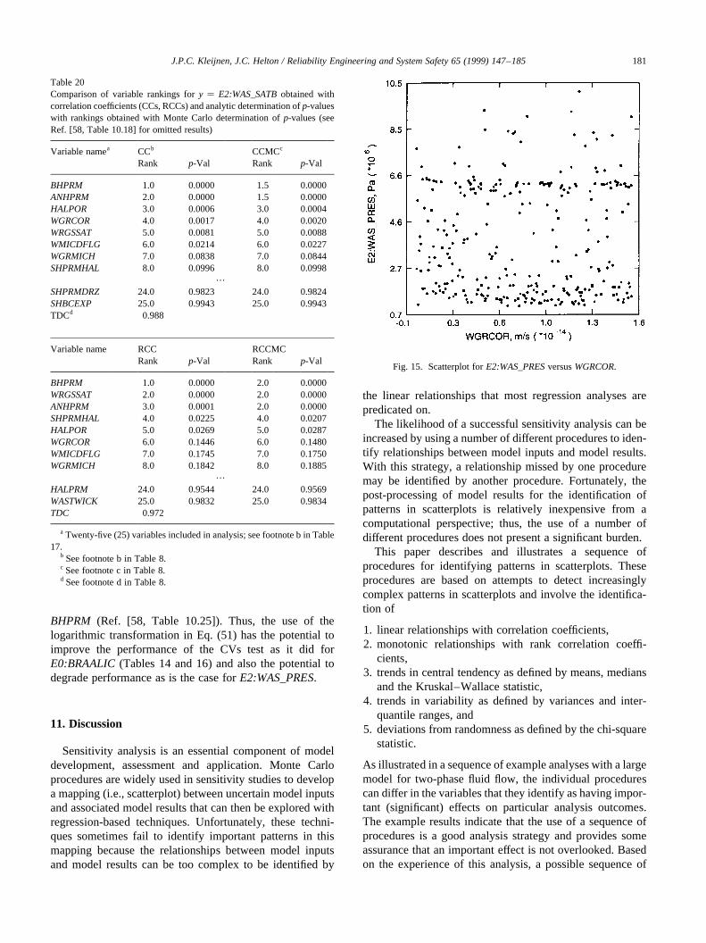
BHPRM (Ref. [58, Table 10.25]). Thus, the use of thelogarithmic transformation in Eq. (51) has the potential toimprove the performance of the CVs test as it did forE0:BRAALIC(Tables 14 and 16) and also the potential todegrade performance as is the case forE2:WAS_PRES.
11. Discussion
Sensitivity analysis is an essential component of modeldevelopment, assessment and application. Monte Carloprocedures are widely used in sensitivity studies to developa mapping (i.e., scatterplot) between uncertain model inputsand associated model results that can then be explored withregression-based techniques. Unfortunately, these techni-ques sometimes fail to identify important patterns in thismapping because the relationships between model inputsand model results can be too complex to be identified by
the linear relationships that most regression analyses arepredicated on.
The likelihood of a successful sensitivity analysis can beincreased by using a number of different procedures to iden-tify relationships between model inputs and model results.With this strategy, a relationship missed by one proceduremay be identified by another procedure. Fortunately, thepost-processing of model results for the identification ofpatterns in scatterplots is relatively inexpensive from acomputational perspective; thus, the use of a number ofdifferent procedures does not present a significant burden.
This paper describes and illustrates a sequence ofprocedures for identifying patterns in scatterplots. Theseprocedures are based on attempts to detect increasinglycomplex patterns in scatterplots and involve the identifica-tion of
1. linear relationships with correlation coefficients,2. monotonic relationships with rank correlation coeffi-
cients,3. trends in central tendency as defined by means, medians
and the Kruskal–Wallace statistic,4. trends in variability as defined by variances and inter-
quantile ranges, and5. deviations from randomness as defined by the chi-square
statistic.
As illustrated in a sequence of example analyses with a largemodel for two-phase fluid flow, the individual procedurescan differ in the variables that they identify as having impor-tant (significant) effects on particular analysis outcomes.The example results indicate that the use of a sequence ofprocedures is a good analysis strategy and provides someassurance that an important effect is not overlooked. Basedon the experience of this analysis, a possible sequence of
J.P.C. Kleijnen, J.C. Helton / Reliability Engineering and System Safety 65 (1999) 147–185 181
Table 20Comparison of variable rankings fory � E2:WAS_SATBobtained withcorrelation coefficients (CCs, RCCs) and analytic determination ofp-valueswith rankings obtained with Monte Carlo determination ofp-values (seeRef. [58, Table 10.18] for omitted results)
Variable namea CCb CCMCc
Rank p-Val Rank p-Val
BHPRM 1.0 0.0000 1.5 0.0000ANHPRM 2.0 0.0000 1.5 0.0000HALPOR 3.0 0.0006 3.0 0.0004WGRCOR 4.0 0.0017 4.0 0.0020WRGSSAT 5.0 0.0081 5.0 0.0088WMICDFLG 6.0 0.0214 6.0 0.0227WGRMICH 7.0 0.0838 7.0 0.0844SHPRMHAL 8.0 0.0996 8.0 0.0998
…
SHPRMDRZ 24.0 0.9823 24.0 0.9824SHBCEXP 25.0 0.9943 25.0 0.9943TDCd 0.988
Variable name RCC RCCMCRank p-Val Rank p-Val
BHPRM 1.0 0.0000 2.0 0.0000WRGSSAT 2.0 0.0000 2.0 0.0000ANHPRM 3.0 0.0001 2.0 0.0000SHPRMHAL 4.0 0.0225 4.0 0.0207HALPOR 5.0 0.0269 5.0 0.0287WGRCOR 6.0 0.1446 6.0 0.1480WMICDFLG 7.0 0.1745 7.0 0.1750WGRMICH 8.0 0.1842 8.0 0.1885
…
HALPRM 24.0 0.9544 24.0 0.9569WASTWICK 25.0 0.9832 25.0 0.9834TDC 0.972
a Twenty-five (25) variables included in analysis; see footnote b in Table17.
b See footnote b in Table 8.c See footnote c in Table 8.d See footnote d in Table 8.
Fig. 15. Scatterplot forE2:WAS_PRESversusWGRCOR.
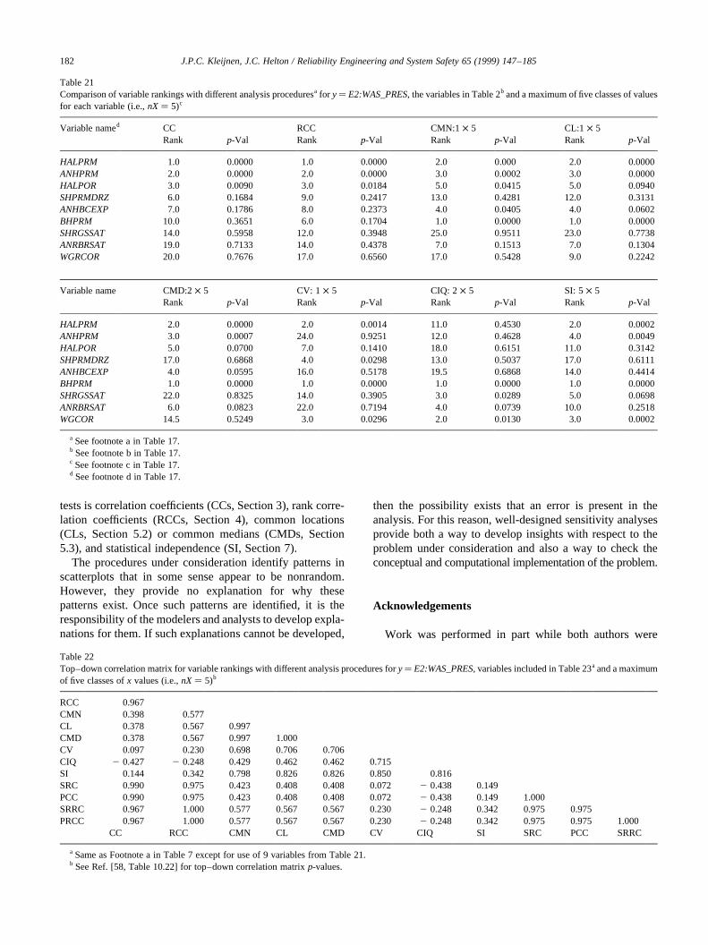
tests is correlation coefficients (CCs, Section 3), rank corre-lation coefficients (RCCs, Section 4), common locations(CLs, Section 5.2) or common medians (CMDs, Section5.3), and statistical independence (SI, Section 7).
The procedures under consideration identify patterns inscatterplots that in some sense appear to be nonrandom.However, they provide no explanation for why thesepatterns exist. Once such patterns are identified, it is theresponsibility of the modelers and analysts to develop expla-nations for them. If such explanations cannot be developed,
then the possibility exists that an error is present in theanalysis. For this reason, well-designed sensitivity analysesprovide both a way to develop insights with respect to theproblem under consideration and also a way to check theconceptual and computational implementation of the problem.
Acknowledgements
Work was performed in part while both authors were
J.P.C. Kleijnen, J.C. Helton / Reliability Engineering and System Safety 65 (1999) 147–185182
Table 21Comparison of variable rankings with different analysis proceduresa for y� E2:WAS_PRES, the variables in Table 2b and a maximum of five classes of valuesfor each variable (i.e.,nX� 5)c
Variable named CC RCC CMN:1× 5 CL:1 × 5Rank p-Val Rank p-Val Rank p-Val Rank p-Val
HALPRM 1.0 0.0000 1.0 0.0000 2.0 0.000 2.0 0.0000ANHPRM 2.0 0.0000 2.0 0.0000 3.0 0.0002 3.0 0.0000HALPOR 3.0 0.0090 3.0 0.0184 5.0 0.0415 5.0 0.0940SHPRMDRZ 6.0 0.1684 9.0 0.2417 13.0 0.4281 12.0 0.3131ANHBCEXP 7.0 0.1786 8.0 0.2373 4.0 0.0405 4.0 0.0602BHPRM 10.0 0.3651 6.0 0.1704 1.0 0.0000 1.0 0.0000SHRGSSAT 14.0 0.5958 12.0 0.3948 25.0 0.9511 23.0 0.7738ANRBRSAT 19.0 0.7133 14.0 0.4378 7.0 0.1513 7.0 0.1304WGRCOR 20.0 0.7676 17.0 0.6560 17.0 0.5428 9.0 0.2242
Variable name CMD:2× 5 CV: 1 × 5 CIQ: 2× 5 SI: 5× 5Rank p-Val Rank p-Val Rank p-Val Rank p-Val
HALPRM 2.0 0.0000 2.0 0.0014 11.0 0.4530 2.0 0.0002ANHPRM 3.0 0.0007 24.0 0.9251 12.0 0.4628 4.0 0.0049HALPOR 5.0 0.0700 7.0 0.1410 18.0 0.6151 11.0 0.3142SHPRMDRZ 17.0 0.6868 4.0 0.0298 13.0 0.5037 17.0 0.6111ANHBCEXP 4.0 0.0595 16.0 0.5178 19.5 0.6868 14.0 0.4414BHPRM 1.0 0.0000 1.0 0.0000 1.0 0.0000 1.0 0.0000SHRGSSAT 22.0 0.8325 14.0 0.3905 3.0 0.0289 5.0 0.0698ANRBRSAT 6.0 0.0823 22.0 0.7194 4.0 0.0739 10.0 0.2518WGCOR 14.5 0.5249 3.0 0.0296 2.0 0.0130 3.0 0.0002
a See footnote a in Table 17.b See footnote b in Table 17.c See footnote c in Table 17.d See footnote d in Table 17.
Table 22Top–down correlation matrix for variable rankings with different analysis procedures fory� E2:WAS_PRES, variables included in Table 23a and a maximumof five classes ofx values (i.e.,nX� 5)b
RCC 0.967CMN 0.398 0.577CL 0.378 0.567 0.997CMD 0.378 0.567 0.997 1.000CV 0.097 0.230 0.698 0.706 0.706CIQ 2 0.427 2 0.248 0.429 0.462 0.462 0.715SI 0.144 0.342 0.798 0.826 0.826 0.850 0.816SRC 0.990 0.975 0.423 0.408 0.408 0.072 2 0.438 0.149PCC 0.990 0.975 0.423 0.408 0.408 0.072 2 0.438 0.149 1.000SRRC 0.967 1.000 0.577 0.567 0.567 0.230 2 0.248 0.342 0.975 0.975PRCC 0.967 1.000 0.577 0.567 0.567 0.230 2 0.248 0.342 0.975 0.975 1.000
CC RCC CMN CL CMD CV CIQ SI SRC PCC SRRC
a Same as Footnote a in Table 7 except for use of 9 variables from Table 21.b See Ref. [58, Table 10.22] for top–down correlation matrixp-values.
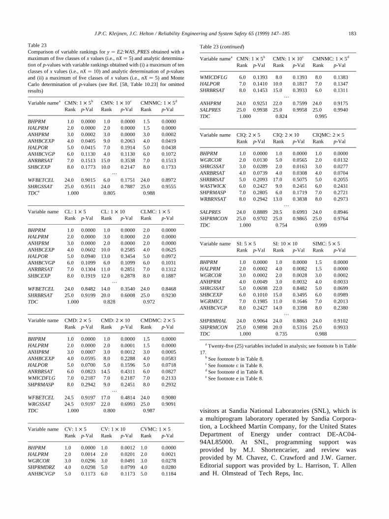
visitors at Sandia National Laboratories (SNL), which isa multiprogram laboratory operated by Sandia Corpora-tion, a Lockheed Martin Company, for the United StatesDepartment of Energy under contract DE-AC04-94AL85000. At SNL, programming support wasprovided by M.J. Shortencarier, and review wasprovided by M. Chavez, C. Crawford and J.W. Garner.Editorial support was provided by L. Harrison, T. Allenand H. Olmstead of Tech Reps, Inc.
J.P.C. Kleijnen, J.C. Helton / Reliability Engineering and System Safety 65 (1999) 147–185 183
Table 23Comparison of variable rankings fory � E2:WAS_PRESobtained with amaximum of five classes ofx values (i.e.,nX� 5) and analytic determina-tion of p-values with variable rankings obtained with (i) a maximum of tenclasses ofx values (i.e.,nX� 10) and analytic determination ofp-valuesand (ii) a maximum of five classes ofx values (i.e.,nX � 5) and MonteCarlo determination ofp-values (see Ref. [58, Table 10.23] for omittedresults)
Variable namea CMN: 1 × 5b CMN: 1 × 10c CMNMC: 1 × 5d
Rank p-Val Rank p-Val Rank p-Val
BHPRM 1.0 0.0000 1.0 0.0000 1.5 0.0000HALPRM 2.0 0.0000 2.0 0.0000 1.5 0.0000ANHPRM 3.0 0.0002 3.0 0.0000 3.0 0.0002ANHBCEXP 4.0 0.0405 9.0 0.2063 4.0 0.0419HALPOR 5.0 0.0415 7.0 0.1914 5.0 0.0438ANHBCVGP 6.0 0.1130 4.0 0.1130 6.0 0.1072ANRBRSAT 7.0 0.1513 15.0 0.3538 7.0 0.1513SHBCEXP 8.0 0.1773 10.0 0.2147 8.0 0.1733
…
WFBETCEL 24.0 0.9015 6.0 0.1751 24.0 0.8972SHRGSSAT 25.0 0.9511 24.0 0.7887 25.0 0.9555TDCe 1.000 0.805 0.988
Variable name CL: 1× 5 CL: 1 × 10 CLMC: 1× 5Rank p-Val Rank p-Val Rank p-Val
BHPRM 1.0 0.0000 1.0 0.0000 2.0 0.0000HALPRM 2.0 0.0000 3.0 0.0000 2.0 0.0000ANHPRM 3.0 0.0000 2.0 0.0000 2.0 0.0000ANHBCEXP 4.0 0.0602 10.0 0.2585 4.0 0.0625HALPOR 5.0 0.0940 13.0 0.3454 5.0 0.0972ANHBCVGP 6.0 0.1099 6.0 0.1099 6.0 0.1031ANRBRSAT 7.0 0.1304 11.0 0.2851 7.0 0.1312SHBCEXP 8.0 0.1919 12.0 0.2878 8.0 0.1887
…
WFBETCEL 24.0 0.8482 14.0 0.3540 24.0 0.8468SHRBRSAT 25.0 0.9199 20.0 0.6008 25.0 0.9230TDC 1.000 0.828 0.972
Variable name CMD: 2× 5 CMD: 2 × 10 CMDMC: 2× 5Rank p-Val Rank p-Val Rank p-Val
BHPRM 1.0 0.0000 1.0 0.0000 1.5 0.0000HALPRM 2.0 0.0000 2.0 0.0001 1.5 0.0000ANHPRM 3.0 0.0007 3.0 0.0012 3.0 0.0005ANHBCEXP 4.0 0.0595 8.0 0.2288 4.0 0.0583HALPOR 5.0 0.0700 5.0 0.1596 5.0 0.0718ANRBRSAT 6.0 0.0823 14.5 0.4311 6.0 0.0827WMICDFLG 7.0 0.2187 7.0 0.2187 7.0 0.2133SHPRMASP 8.0 0.2942 9.0 0.2451 8.0 0.2932
…
WFBETCEL 24.5 0.9197 17.0 0.4814 24.0 0.9080WRGSSAT 24.5 0.9197 22.0 0.6993 25.0 0.9091TDC 1.000 0.800 0.987
Variable name CV: 1× 5 CV: 1 × 10 CVMC: 1× 5Rank p-Val Rank p-Val Rank p-Val
BHPRM 1.0 0.0000 1.0 0.0012 1.0 0.0000HALPRM 2.0 0.0014 2.0 0.0201 2.0 0.0021WGRCOR 3.0 0.0296 3.0 0.0491 3.0 0.0278SHPRMDRZ 4.0 0.0298 5.0 0.0799 4.0 0.0280ANHBCVGP 5.0 0.1173 6.0 0.1173 5.0 0.1184
Table 23 (continued)
Variable namea CMN: 1 × 5b CMN: 1 × 10c CMNMC: 1 × 5d
Rank p-Val Rank p-Val Rank p-Val
WMICDFLG 6.0 0.1393 8.0 0.1393 8.0 0.1383HALPOR 7.0 0.1410 10.0 0.1817 7.0 0.1347SHRBRSAT 8.0 0.1453 15.0 0.3933 6.0 0.1311
…
ANHPRM 24.0 0.9251 22.0 0.7599 24.0 0.9175SALPRES 25.0 0.9938 25.0 0.9958 25.0 0.9940TDC 1.000 0.824 0.995
Variable name CIQ: 2× 5 CIQ: 2× 10 CIQMC: 2× 5Rank p-Val Rank p-Val Rank p-Val
BHPRM 1.0 0.0000 1.0 0.0000 1.0 0.0000WGRCOR 2.0 0.0130 5.0 0.0565 2.0 0.0132SHRGSSAT 3.0 0.0289 2.0 0.0163 3.0 0.0277ANRBRSAT 4.0 0.0739 4.0 0.0308 4.0 0.0704SHRBRSAT 5.0 0.2093 17.0 0.5075 5.0 0.2055WASTWICK 6.0 0.2427 9.0 0.2451 6.0 0.2431SHPRMASP 7.0 0.2805 6.0 0.1719 7.0 0.2721WRBRNSAT 8.0 0.2942 13.0 0.3838 8.0 0.2973
…
SALPRES 24.0 0.8889 20.5 0.6993 24.0 0.8946SHPRMCON 25.0 0.9702 25.0 0.9865 25.0 0.9764TDC 1.000 0.754 0.999
Variable name SI: 5× 5 SI: 10× 10 SIMC: 5× 5Rank p-Val Rank p-Val Rank p-Val
BHPRM 1.0 0.0000 1.0 0.0000 1.5 0.0000HALPRM 2.0 0.0002 4.0 0.0082 1.5 0.0000WGRCOR 3.0 0.0002 2.0 0.0028 3.0 0.0002ANHPRM 4.0 0.0049 3.0 0.0032 4.0 0.0033SHRGSSAT 5.0 0.0698 22.0 0.8482 5.0 0.0699SHBCEXP 6.0 0.1010 15.0 0.3495 6.0 0.0989WGRMICI 7.0 0.1985 11.0 0.1646 7.0 0.2013ANHBCVGP 8.0 0.2427 14.0 0.3398 8.0 0.2380
…
SHPRMHAL 24.0 0.9064 24.0 0.8863 24.0 0.9102SHPRMCON 25.0 0.9898 20.0 0.5316 25.0 0.9933TDC 1.000 0.735 0.988
a Twenty-five (25) variables included in analysis; see footnote b in Table17.
b See footnote b in Table 8.c See footnote c in Table 8.d See footnote d in Table 8.e See footnote e in Table 8.
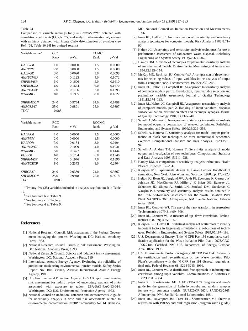
References
[1] National Research Council. Risk assessment in the Federal Govern-ment: managing the process. Washington, DC: National AcademyPress, 1983.
[2] National Research Council. Issues in risk assessment. Washington,DC: National Academy Press, 1993.
[3] National Research Council. Science and judgment in risk assessment.Washington, DC: National Academy Press, 1994.
[4] International Atomic Energy Agency. Evaluating the reliability ofpredictions made using environmental transfer models. Safety SeriesReport No. 100. Vienna, Austria: International Atomic EnergyAgency, 1989.
[5] U.S. Environmental Protection Agency. An SAB report: multi-mediarisk assessment for radon, review of uncertainty analysis of risksassociated with exposure to radon. EPA-SAB-RAC-93-014.Washington, DC: U.S. Environmental Protection Agency, 1993.
[6] National Council on Radiation Protection and Measurements. A guidefor uncertainty analysis in dose and risk assessments related toenvironmental contamination. NCRP Commentary No. 14. Bethesda,
MD: National Council on Radiation Protection and Measurements,1996.
[7] Iman RL, Helton JC. An investigation of uncertainty and sensitivityanalysis techniques for computer models. Risk Analysis 1988;8:71–90.
[8] Helton JC. Uncertainty and sensitivity analysis techniques for use inperformance assessment of radioactive waste disposal. ReliabilityEngineering and System Safety 1993;42:327–367.
[9] Hamby DM. A review of techniques for parameter sensitivity analysisof environmental models. Environmental Monitoring and Assessment1994;32:125–154.
[10] McKay MD, Beckman RJ, Conover WJ. A comparison of three meth-ods for selecting values of input variables in the analysis of outputfrom a computer code. Technometrics 1979;21:239–245.
[11] Iman RL, Helton JC, Campbell JE. An approach to sensitivity analysisof computer models, part 1. Introduction, input variable selection andpreliminary variable assessment. Journal of Quality Technology1981;13:174–183.
[12] Iman RL, Helton JC, Campbell JE. An approach to sensitivity analysisof computer models, part 2. Ranking of input variables, responsesurface validation, distribution effect and technique synopsis. Journalof Quality Technology 1981;13:232–240.
[13] Saltelli A, Marivoet J. Non-parametric statistics in sensitivity analysisfor model output: a comparison of selected techniques. ReliabilityEngineering and System Safety 1990;28:229–253.
[14] Saltelli A, Homma T. Sensitivity analysis for model output: perfor-mance of black box techniques on three international benchmarkexercises. Computational Statistics and Data Analysis 1992;13:73–94.
[15] Saltelli A, Andres TH, Homma T. Sensitivity analysis of modeloutput: an investigation of new techniques. Computational Statisticsand Data Analysis 1993;15:211–238.
[16] Hamby DM. A comparison of sensitivity analysis techniques. HealthPhysics 1995;68:195–204.
[17] Kleijnen JPC. Experimental design. In: Banks J, editor. Handbook ofsimulation, New York: John Wiley and Sons Inc, 1998. pp. 173–223.
[18] Helton JC, Bean JE, Berglund JW, Davis FJ, Economy K, Garner JW,Johnson JD, MacKinnon RJ, Miller J, O’Brien DG, Ramsey JL,Schreiber JD, Shinta A, Smith LN, Stoelzel DM, Stockman C,Vaughn P. Uncertainty and sensitivity analysis results obtained inthe 1996 performance assessment for the Waste Isolation PilotPlant. SAND98-0365. Albuquerque, NM: Sandia National Labora-tories, 1998.
[19] Iman RL, Conover WJ. The use of the rank transform in regression.Technometrics 1979;21:499–509.
[20] Iman RL, Conover WJ. A measure of top–down correlation. Techno-metrics 1987;29(3):351–357.
[21] Kleijnen JPC, Helton JC. Statistical analyses of scatterplots to identifyimportant factors in large-scale simulations, 2: robustness of techni-ques. Reliability Engineering and System Safety 1999;65:187–198.
[22] U.S. Department of Energy. Title 40 CFR Part 191 compliance certi-fication application for the Waste Isolation Pilot Plant. DOE/CAO-1996-2184: Carlsbad, NM: U.S. Department of Energy, CarlsbadArea Office, 1996.
[23] U.S. Environmental Protection Agency. 40 CFR Part 194: Criteria forthe certification and re-certification of the Waste Isolation PilotPlant’s compliance with the 40 CFR Part 191 disposal regulations;final rule. Federal Register 61: 5224-5245, 1996.
[24] Iman RL, Conover WJ. A distribution-free approach to inducing rankcorrelation among input variables. Communications in Statistics B1982;11:311–334.
[25] Iman RL, Shortencarier MJ. A FORTRAN 77 program and user’sguide for the generation of Latin hypercube and random samplesfor use with computer models. NUREG/CR-2624, SAND83-2365.Albuquerque, NM: Sandia National Laboratories, 1984.
[26] Iman RL, Davenport JM, Frost EL, Shortencarier MJ. Stepwiseregression with PRESS and rank regression (program user’s guide).
J.P.C. Kleijnen, J.C. Helton / Reliability Engineering and System Safety 65 (1999) 147–185184
Table 24Comparison of variable rankings fory � E2:WAS(PRESobtained withcorrelation coefficients (CCs, RCCs) and analytic determination ofp-valueswith rankings obtained with Monte Carlo determination ofp-values (seeRef. [58, Table 10.24] for omitted results)
Variable namea CCb CCMCc
Rank p-Val Rank p-Val
HALPRM 1.0 0.0000 1.5 0.0000ANHPRM 2.0 0.0000 1.5 0.0000HALPOR 3.0 0.0090 3.0 0.0098ANHBCVGP 4.0 0.1123 4.0 0.1072SHPRMASP 5.0 0.1606 5.0 0.1610SHPRMDRZ 6.0 0.1684 6.0 0.1670ANHBCEXP 7.0 0.1786 7.0 0.1795WGRMICI 8.0 0.1905 8.0 0.1827
…
SHPRMCON 24.0 0.9794 24.0 0.9798ANRGSSAT 25.0 0.9891 25.0 0.9897TDCd 0.988
Variable name RCC RCCMCRank p-Val Rank p-Val
HALPRM 1.0 0.0000 1.5 0.0000ANHPRM 2.0 0.0000 1.5 0.0000HALPOR 3.0 0.0184 3.0 0.0194ANHBCVGP 4.0 0.1099 4.0 0.1031WGRMICI 5.0 0.1477 5.0 0.1444BHPRM 6.0 0.1704 6.0 0.1746SHPRMASP 7.0 0.1946 7.0 0.1896ANHBCEXP 8.0 0.2373 8.0 0.2404
…
SHBCEXP 24.0 0.9389 24.0 0.9367SHPRMCON 25.0 0.9918 25.0 0.9918TDC 0.988
a Twenty-five (25) variables included in analysis; see footnote b in Table17.
b See footnote b in Table 9.c See footnote c in Table 9.d See footnote d in Table 9.

SAND79-1472. Albuquerque, NM: Sandia National Laboratories,1980.
[27] Draper NR, Smith H. Applied regression analysis. 2nd edition. NewYork: John Wiley and Sons, Inc, 1981.
[28] Myers RH. Classical and modern regression with applications.Belmont, CA: Duxbury Press, 1989.
[29] Press WH, Teukolsky SA, Vetterlings WT, Flannery BP. Numericalrecipes: the art of scientific computing (FORTRAN version). 2ndedition. Cambridge: Cambridge University Press, 1992.
[30] Chan MS. The consequences of uncertainty for the prediction of theeffects of schistosomiasis control programmes. Epidemiology andInfection 1996;117:537–550.
[31] Ma JZ, Ackerman E, Yang JJ. Parameter sensitivity of a model ofviral epidemics simulated with Monte Carlo techniques. I. Illnessattack rates. International Journal of Biomedical Computing1993;32:237–253.
[32] Ma JZ, Ackerman E. Parameter sensitivity of a model of viralepidemics simulated with Monte Carlo techniques, II. Durationsand peaks. International Journal of Biomedical Computing1993;32:255–268.
[33] Whiting WB, Tong TM, Reed ME. Effect of uncertainties in thermo-dynamic data and model parameters on calculated process perfor-mance. Industrial and Engineering Chemistry Research1993;32:1367–1371.
[34] Breshears D, Kirchner TB, Whicker FW. Contaminant transportthrough agro-ecosystems: assessing relative importance of environ-mental, physiological and management factors. Ecological Applica-tions 1992;2(3):285–297.
[35] Iman RL, Shortencarier MJ, Johnson JD. A FORTRAN 77 programand user’s guide for the calculation of partial correlation and standar-dized regression coefficients. NUUREG/CR-4122. SAND85-0044.Albuquerque, NM: Sandia National Laboratories, 1985.
[36] Helton JC, Garner JW, McCurley RD, Rudeen DK. Sensitivity analy-sis techniques and results for performance assessment at the WasteIsolation Pilot Plant. SAND90-7103. Albuquerque, NM: SandiaNational Laboratories, 1991.
[37] Conover WJ. Practical non-parametric statistics. 2nd edition. NewYork: John Wiley and Sons Inc, 1980.
[38] Sanchez MA, Blower SM. Uncertainty and sensitivity analysis of thebasic reproductive rate: tuberculosis as an example. American Journalof Epidemiology 1997;145(12):1127–1137.
[39] Gwo JP, Toran LE, Morris MD, Wilson GV. Subsurface stormflowmodeling with sensitivity analysis using a Latin-hypercube samplingtechnique. Groundwater 1996;34:811–818.
[40] Helton JC, et al. Uncertanity and sensitivity analysis resultsobtained in the 1992 performance assessment for the WasteIsolation Pilot Plant. Reliability Engineering and System Safety1996;51:53–100.
[41] Blower SM, Dowlatabadi H. Sensitivity and uncertainty analysis ofcomplex models of disease transmission: an HIV model, as anexample. International Statistical Review 1994;62(2):229–243.
[42] MacDonald RC, Campbell JE. Valuation of supplemental andenhanced oil recovery projects with risk analysis. Journal of Petro-leum Technology 1986;38:57–69.
[43] Andrews DF, Bickel PJ, Hample FR, Huber P, Rogers W, Tukey J.Robust estimates of location. Princeton: Princeton University Press,1972.
[44] ScheffeH. The analysis of variance. New York: John Wiley and Sons,Inc, 1959.
[45] Kleijnen JPC. Statistical tools for simulation practitioners. New York:Marcel Dekker, 1987.
[46] D’Agostino RD, Stephens HA. Goodness-of-fit distributions. NewYork: Marcel Dekker, 1986.
[47] David HA. Order statistics. 2nd edition. New York: John Wiley andSons, 1981.
[48] Sargent RG. Some subjective validation methods using graphicaldisplays of data. In: Charnes JM, Morrice DJ, Brunner DT, SwainJJ, editors. 1996 Winter Simulation Conference Proceedings. Piscat-away, NJ: Institute of Electrical and Electronics Engineers, 1996, pp.345–351.
[49] Conover WJ, Johnson ME, Johnson MM. A comparative study of testsfor homogeneity of variances, with applications to the outer continen-tal shelf bidding data. Technometrics 1981;23(1):351–361.
[50] Piepho H-P. Tests for equality of dispersion in bivariate samples –review and empirical comparison. Journal of Statistical Computationand Simulation 1997;56:353–372.
[51] Wludyka PS, Nelson PR. Analysis of means type tests for variancesusing subsampling and jackknifing. American Journal of Mathemati-cal and Management Sciences 1997;17:31–60.
[52] Efron B. The jackknife, the bootstrap and other resampling plans.Philadelphia: CBMS-NSF Series, Siam, 1982.
[53] Miller RG. The jackknife — a review. Biometrika 1974;61:1–15.[54] Archer GEB, Saltelli A, Sobol TM. Sensitivity measures, ANOVA-
like techniques and the use of bootstrap. Journal of Statistical Compu-tation and Simulation 1997;58:99–120.
[55] Helton JC. Uncertainty and sensitivity analysis in the presence ofstochastic and subjective uncertainty. Journal of Statistical Computa-tion and Simulation 1997;57:3–76.
[56] Iman RL. Tables of the exact quantiles of the top–down correlationcoefficient forn � 3(1)14. Communications in Statistics — Theoryand Methods 1987;16:1513–1540.
[57] Efron B, Tibshirani RJ. Introduction to the bootstrap. London: Chap-man and Hall, 1993.
[58] Kleijnen JPC, Helton JC. Statistical analyses of scatterplots to identifyimportant factors in large-scale simulations. SAND98-2202. Albu-querque, NM: Sandia National Laboratories, 1999.
J.P.C. Kleijnen, J.C. Helton / Reliability Engineering and System Safety 65 (1999) 147–185 185