STATISTICA Scorecard Formula Guide guide/STATISTICA... · STATISTICA Scorecard is a comprehensive tool dedicated for developing, evaluating, and monitoring scorecard models. For more

STATISTICA Formula Guide

STATISTICA Scorecard

Copyright 2013 ̶ Version 1 PAGE 1 OF 32

Making the World More Productive®

Formula Guide


STATISTICA Scorecard is a comprehensive tool dedicated for developing, evaluating, and monitoring

scorecard models. For more information see TUTORIAL Developing Scorecards Using STATISTICA

Scorecard [4]. STATISTICA Scorecard is an add-in for STATISTICA Data Miner and on the computation

level is based on native STATISTICA algorithms such as: Logistic regression, Decision trees (CART and

CHAID), Factor analysis, Random forest and Cox regression. The document contains formulas and

algorithms that are beyond of the scope of the implemented natively in STATISTICA.





Contents

Feature selection ........................................................................................................................................ 5

Feature selection – Cramer’s V ............................................................................................................... 6

Notation .................................................................................................................................................. 6

Computation Details ............................................................................................................................... 6

Feature selection – (IV) Information Value ............................................................................................ 7

Notation .................................................................................................................................................. 7


Feature selection – Gini .......................................................................................................................... 8


Interaction and Rules .................................................................................................................................. 9

Interaction and Rules – Bad rate (and Good rate) .................................................................................. 9

Notation ................................................................................................................................................ 10

Interaction and Rules – Lift (bad) and Lift (good) ................................................................................. 11

Notation ................................................................................................................................................ 11

Attribute building ...................................................................................................................................... 12

Attribute building – (WoE) Weight of Evidence ................................................................................... 12

Notation ................................................................................................................................................ 12

Computation Details ............................................................................................................................. 12

Scorecard preparation .............................................................................................................................. 13

Scorecard preparation – Scaling – Factor ............................................................................................. 13

Notation ................................................................................................................................................ 13

Scorecard preparation – Scaling – Offset ............................................................................................. 14

Notation ................................................................................................................................................ 14

Scorecard preparation – Scaling –Calculating score (WoE coding) ...................................................... 15

Notation ................................................................................................................................................ 15


Scorecard preparation – Scaling –Calculating score (Dummy coding) ................................................. 16

Notation ................................................................................................................................................ 16


Scorecard preparation – Scaling – Neutral score ................................................................................. 17





Notation ................................................................................................................................................ 17

Scorecard preparation – Scaling – Intercept adjustment ..................................................................... 18

Notation ................................................................................................................................................ 18

Survival ...................................................................................................................................................... 19

Reject Inference ........................................................................................................................................ 20

Reject Inference - Parceling method .................................................................................................... 20

Model evaluation ...................................................................................................................................... 21

Model evaluation – Gini ........................................................................................................................ 21

Notation ................................................................................................................................................ 21


Model evaluation – Information Value (IV) .......................................................................................... 21

Model evaluation - Divergence ............................................................................................................. 22

Notation ................................................................................................................................................ 22

Model evaluation – Hosmer-Lemeshow ............................................................................................... 23

Notation ................................................................................................................................................ 23


Model evaluation – Kolmogorov-Smirnov statistic .............................................................................. 24

Notation ................................................................................................................................................ 24


Comments ............................................................................................................................................. 24

Model evaluation – AUC – Area Under ROC Curve .............................................................................. 25

Notation ................................................................................................................................................ 25

Model evaluation – 2x2 tables measures ............................................................................................. 26

Notation ................................................................................................................................................ 26

Cut-off point selection .............................................................................................................................. 27

Cut-off point selection – ROC optimal cut-off point ............................................................................. 27

Notation ................................................................................................................................................ 27

Score cases ................................................................................................................................................ 28

Score cases – Adjusting probabilities .................................................................................................... 28

Notation ................................................................................................................................................ 28

Calibration tests ........................................................................................................................................ 29






Population stability ................................................................................................................................... 30

Population stability ............................................................................................................................... 30

Notation ................................................................................................................................................ 30

Characteristic stability .......................................................................................................................... 31

Notation ................................................................................................................................................ 31

References ................................................................................................................................................ 32





Feature selection

The Feature Selection module is used to exclude unimportant or redundant variables from the initial

set of characteristics. Select representatives option enable you to identify redundancy among

numerical variables without analyzing the correlation matrix of all variables. This module creates

bundles of commonly correlated characteristics using Factor analysis with principal components

extraction method and optional factor rotation that is implemented as standard STATISTICA procedure.

Bundles of variables are created based on value of factor loadings (correlation between given variable

and particular factor score) User can set the option defining minimal absolute value of loading that

makes given variable representative of particular factor. Number of components is defined based on

eingenvalue or max factors option. If categorical predictors are selected before factor calculation

variables are recoded using WoE (log odds) transformation (described in the Attribute Building

chapter).

In each bundle, variables are highly correlated with the same factor (in other words have high absolute

value of factor loading) and often with each other, so we can easily select only a small number of

bundle representatives. After bundles are identified user can manually or automatically select

representatives of each bundle. In case of automatic selection user can select correlation option that

allows selecting variables with the highest correlation with other variables in given bundle. The other

option is IV criterion (described below).

Variable rankings can be created using three measures of overall predictive power of variables: IV

(Information Value), Cramer’s V, and the Gini coefficient. Based on these measures, you can identify

the characteristics that have an important impact on credit risk and select them for the next stage of

model development. For more information see TUTORIAL Developing Scorecards Using STATISTICA

Scorecard [4].





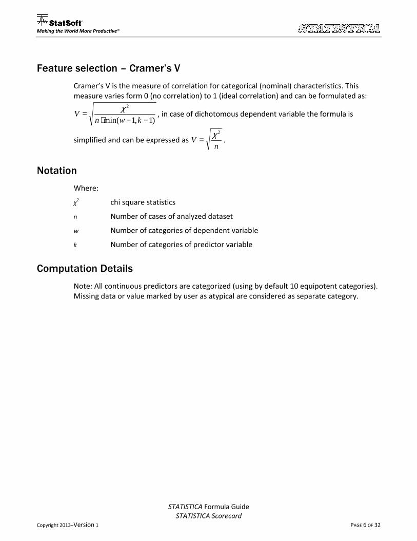
Feature selection – Cramer’s V

Cramer’s V is the measure of correlation for categorical (nominal) characteristics. This

measure varies form 0 (no correlation) to 1 (ideal correlation) and can be formulated as:

)1,1min(

2

−−⋅=

kwnV

χ, in case of dichotomous dependent variable the formula is

simplified and can be expressed as n

V2χ= .

Notation

Where:

χ2 chi square statistics

n Number of cases of analyzed dataset

w Number of categories of dependent variable

k Number of categories of predictor variable

Computation Details

Note: All continuous predictors are categorized (using by default 10 equipotent categories).

Missing data or value marked by user as atypical are considered as separate category.





Feature selection – (IV) Information Value

Information Value is an indicator of the overall predictive power of the characteristic. We

can compute this measure as: ( ) 100ln1

⋅

⋅−= ∑

= i

ik

iii b

gbgIV

Notation

Where:

k number of bins (attributes) of analyzed predictor

gi column-wise percentage distribution of the total “good” cases in the ith

bin

bi column-wise percentage distribution of the total “bad” cases in the ith

bin

Computation Details







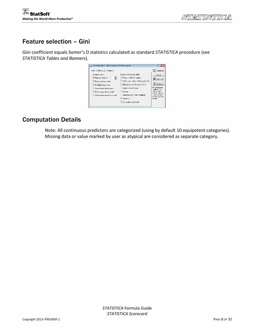
Feature selection – Gini

Gini coefficient equals Somer’s D statistics calculated as standard STATISTICA procedure (see

STATISTICA Tables and Banners).

Computation Details







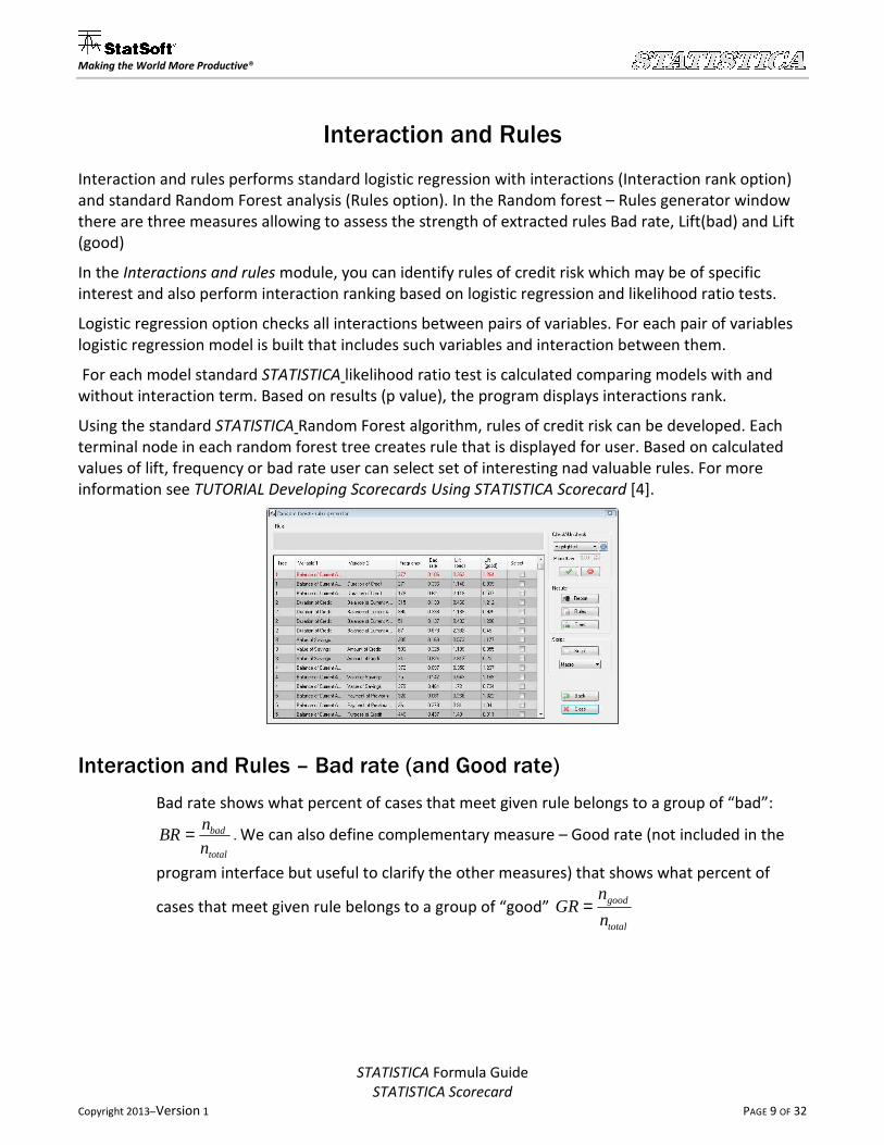
Interaction and Rules

Interaction and rules performs standard logistic regression with interactions (Interaction rank option)

and standard Random Forest analysis (Rules option). In the Random forest – Rules generator window

there are three measures allowing to assess the strength of extracted rules Bad rate, Lift(bad) and Lift

(good)

In the Interactions and rules module, you can identify rules of credit risk which may be of specific

interest and also perform interaction ranking based on logistic regression and likelihood ratio tests.

Logistic regression option checks all interactions between pairs of variables. For each pair of variables

logistic regression model is built that includes such variables and interaction between them.

For each model standard STATISTICA likelihood ratio test is calculated comparing models with and

without interaction term. Based on results (p value), the program displays interactions rank.

Using the standard STATISTICA Random Forest algorithm, rules of credit risk can be developed. Each

terminal node in each random forest tree creates rule that is displayed for user. Based on calculated

values of lift, frequency or bad rate user can select set of interesting nad valuable rules. For more

information see TUTORIAL Developing Scorecards Using STATISTICA Scorecard [4].

Interaction and Rules – Bad rate (and Good rate)

Bad rate shows what percent of cases that meet given rule belongs to a group of “bad”:

total

bad

n

nBR = . We can also define complementary measure – Good rate (not included in the

program interface but useful to clarify the other measures) that shows what percent of

cases that meet given rule belongs to a group of “good” total

good

n

nGR =





Notation

Where:

nbad number of “bad” cases that meet given rule

ngood number of “good” cases that meet given rule

ntotal total number of cases that meet given rule





Interaction and Rules – Lift (bad) and Lift (good)

You can calculate Lift (bad) as a ratio between “bad rate” calculated for a subset of cases

that meet given rule and “bad rate” for the whole dataset. We can express Lift(bad) using

the following formula: Dataset

Rule

BR

BRbadLift =)( .

You can calculate Lift (good) as a ratio between “good rate” calculated for a subset of cases

that meet given rule and “good rate” calculated for the whole dataset. We can express

Lift(good) using the following formula: Dataset

Rule

GR

GRgoodLift =)( .

Notation

Where:

BRRule Bad rate calculated for a subset of cases that meet given rule

BRDataset Bad rate for the whole dataset

GRRule Good rate calculated for a subset of cases that meet given rule

GRDataset Good rate for the whole dataset





Attribute building

In the Attribute Building module, risk profiles for every variable can be prepared. Using an automatic

algorithm based on the standard STATISTICA CHAID, C&RT or CHAID on C&RT methods; manual mode;

percentiles or minimum frequency, we can divide variables (otherwise referred to characteristics) into

classes (attributes or “bins”) containing homogenous risks. Initial attributes can be adjusted manually

to fulfill business and statistical criteria such as profile smoothness or ease of interpretation. There is

also an option to build attributes automatically. To build proper risk profiles, statistical measures of the

predictive power of each attribute (Weight of Evidence (WoE) and IV – Information Value) are

calculated.

If automatic creation of attributes is selected program can find optimal bins using CHAID or C&RT

algorithm. In such case tree models are built for each predictor separately (in other words, each model

contains only one predictor). Attributes are created based on terminal nodes prepared by particular

tree. For continuous predictors there is also option CHAID on C&RT which creates initial attributes

based on C&RT algorithm. Terminal nodes created by C&RT are inputs to CHAID method that tries to

merge similar categories into more overall bins. All options of C&RT and CHAID methods are described

in STATISTICA Help (Interactive Trees (C&RT, CHAID)) [8]. More information see : TUTORIAL Developing

Scorecards Using STATISTICA Scorecard [4].

Attribute building – (WoE) Weight of Evidence

Weight of Evidence (WoE) measures the predictive power of each bin (attribute). We can

compute this measure as: 100)ln( ⋅=b

gWoE .

Notation

Where:

g column-wise percentage distribution of the total “good” cases in analyzed bin

b column-wise percentage distribution of the total “bad” cases in the analyzed bin

Computation Details


If there are atypical values in the variables they are considered as separate bin.

Note: If there are categories without “good” or “bad” categories WoE value is not

calculated. Such category should be merged with adjacent category to avoids errors in

calculations.





Scorecard preparation

The final stage of this process is scorecard preparation using a standard STATISTICA logistic regression

algorithm to estimate model parameters. Options of building logistic regression model like estimation

parameters or stepwise parameters are described in STATISTICA Help (Generalized Linear/Nonlinear

(GLZ) Models) [8].

There are also some scaling transformations and adjustment method that allows the user to calculate

scorecard so the points reflect the real (expected) odds in incoming population. More information see :

TUTORIAL Developing Scorecards Using STATISTICA Scorecard [4].

Scorecard preparation – Scaling – Factor

Factor is one of two scaling parameters used during scorecard calculation process. Factor

can be expressed as:)2ln(

pdoFactor = .

Notation

Where:

pdo Points to double the odds – parameter given by the user





Scorecard preparation – Scaling – Offset

Offset is one of two scaling parameters used during scorecard calculation process. Offset

can be expressed as: ( ))ln(OddsFactorScoreOffset ⋅−=

Notation

Where:

Score scoring value for which you want to receive specific odds of the loan repayment -

parameter given by the user

Odds odds of the loan repayment for specific scoring value - parameter given by the

user

Factor scaling parameter calculated on the basis of formula presented above





Scorecard preparation – Scaling –Calculating score (WoE coding)

When WoE coding is selected for given characteristic, score for each bin (attribute) of such

characteristic is calculated as:m

offsetfactor

mWoEScore +⋅

+⋅= αβ .

Notation

Where:

β logistic regression coefficient for characteristics that owns the given attribute

α logistic regression intercept term

WoE Weight of Evidence value for given attribute

m number of characteristics included in the model

factor scaling parameter based on formula presented previously

offset scaling parameter based on formula presented previously

Computation Details

Note: After computation is complete the resulting value is rounded to the nearest integer

value.





Scorecard preparation – Scaling –Calculating score (Dummy coding)

When dummy coding is selected for given characteristic, score for each bin (attribute) of

such characteristic is calculated as: m

offsetfactor

mScore +⋅

+= αβ .

Notation

Where:

β logistic regression coefficient for the given attribute

α logistic regression intercept term

m number of characteristics included in the model

factor scaling parameter based on formula presented previously

offset scaling parameter based on formula presented previously

Computation Details

Note: After computation is complete the resulting value is rounded to the nearest integer

value.





Scorecard preparation – Scaling – Neutral score

Neutral score is the calculated as: ∑=

⋅=k

iii distrscorescoreNeutral

1

.

Notation

Where:

k number of bins (attributes) of the characteristic

scorei scoring assigned to the ith

bin

distri percentage distribution of the total cases in the ith

bin





Scorecard preparation – Scaling – Intercept adjustment

Balancing data do not effect on regression coefficient except of the intercept (see: Maddala

[3] s. 326). To make score reflect the real data proportions, intercept adjustment is

performed using the following formula: ))ln()(ln( badgoodregressionadjusted pp −−= αα . After

adjustment, calculated intercept value is used during scaling transformation.

Notation

Where:

αregression logistic regression intercept term before adjustment

pgood probability of sampling cases from “good” strata (or class that is coded in logistic

regression as 1)

pbad probability of sampling cases from “bad” strata (or class that is coded in logistic

regression as 0)





Survival

The Survival module is used to build scoring models using the standard STATISTICA Cox Proportional

Hazard Model. We can estimate a scoring model using additional information about the time of

default, or when a debtor stopped paying. Based on this module, we can calculate the probability of

default (scoring) in given time (e.g., after 6 months, 9 months, etc.). Options of input parameters and

output products of Cox Proportional Hazard Model are described in STATISTICA Help (Advanced

Linear/Nonlinear Models - Survival - Regression Models) [8]. For more information see TUTORIAL

Developing Scorecards Using STATISTICA Scorecard [4].





Reject Inference

The Reject inference module allows you to take into consideration cases for which the credit

applications were rejected. Because there is no information about output class (good or bad credit) of

rejected cases, we must add this information using an algorithm. To add information about the output

class, the standard STATISTICA k-nearest neighbors method (from menu Data-Data filtering/Recoding-

MD Imputation) and parceling method are available. After analysis, a new data set with complete

information is produced.

Reject Inference - Parceling method

To use this method preliminary scoring must be calculated for accepted and rejected cases.

After scoring is calculated you must divide score values into certain group with the same

score range. Step option allows you to divide score into group with certain score range and

starting point equal to Starting value parameter, Number of intervals creates given number

of equipotent groups. In each of the groups number of bad and good cases is calculated,

next rejected cases that belong to this score range group are randomly labeled as “bad” or

“good” proportionally to the number of accepted “good” and “bad” in this range.

Business rules often suggest that the ratio of good to bad in a group of rejected applications

should not be the same as in the case of applications approved. User can manually change

the proportion of “good” and “bad” rejected labeled cases in each score range group

separately. One of the rules of thumb suggests that the rejected bad rate should be from

two to four times higher than accepted.





Model evaluation

The Model Evaluation module is used to evaluate and compare different scorecard models. To assess

models, the comprehensive statistical measures can be selected, each with a full detailed report. More

information see : TUTORIAL Developing Scorecards Using STATISTICA Scorecard [4].

Model evaluation – Gini

Gini coefficient measures the extent to which the variable (or model) has better

classification capabilities in comparison to the variable (model) that is a random decision

maker. Gini has a value in the range [0, 1], where 0 corresponds to a random classifier, and

1 is the ideal classifier. We can compute Gini measure as:

( ) ( )∑=

−− +⋅−−=k

iiiii xGxGxBxBG

111 )()()()(1 ; and 0)()( 00 == xBxG

Notation

Where:

k number of categories of analyzed predictor

G(xi) cumulative distribution of “good” cases in the ith

category

B(xi) cumulative distribution of “bad” cases in the ith

category

Computation Details

Note: There is strict relationship between Gini coefficient as AUC (Area Under ROC Curve)

coefficient. Such relationship can be expressed as 12 −⋅= AUCG .

Model evaluation – Information Value (IV)

Information Value (IV) measure is presented in the previous section (feature selection) of

this document.





Model evaluation - Divergence

You can express this index using the following formula: )var(var5,0)( 2

BG

BG meanmeanDivergence

+⋅−= .

Notation

Where:

meanG the mean value of the score in “good” population

meanB the mean value of the score in “bad” population

varG the variance of the score in “good” population

varB the variance of the score in “bad” population





Model evaluation – Hosmer-Lemeshow

Hosmer-Lemeshow goodness of fit statistic is calculated as: ( )

∑= −⋅⋅

⋅−=k

i iii

iii

n

noHL

1

2

)1( πππ

Notation

Where:

k number of groups

oi number of “bad” cases in the ith

group

ni number of cases in the ith

group

iπ average estimated probability of “bad” in the ith

group

Computation Details

Groups for this test are based on the values of the estimated probabilities. In STATISTICA

Scorecard implementation 10 groups are prepared. Groups have the same number of cases.

First group contains subjects having the smallest estimated probabilities and consistently

the last group contains cases having the largest estimated probabilities.





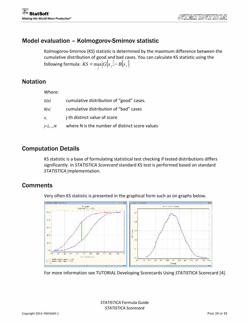
Model evaluation – Kolmogorov-Smirnov statistic

Kolmogorov-Smirnov (KS) statistic is determined by the maximum difference between the

cumulative distribution of good and bad cases. You can calculate KS statistic using the

following formula: ( ) ( )jjj

xBxGKS −= max

Notation

Where:

G(x) cumulative distribution of “good” cases.

B(x) cumulative distribution of “bad” cases

xj j-th distinct value of score

j=1,…,N where N is the number of distinct score values

Computation Details

KS statistic is a base of formulating statistical test checking if tested distributions differs

significantly. In STATISTICA Scorecard standard KS test is performed based on standard

STATISTICA implementation.

Comments

Very often KS statistic is presented in the graphical form such as on graphs below.

For more information see TUTORIAL Developing Scorecards Using STATISTICA Scorecard [4].





Model evaluation – AUC – Area Under ROC Curve

AUC measure can be calculated on the basis of Gini coefficient and can be expressed as:

21+= G

AUC .

Notation

Where:

G Gini coefficient calculated for analyzed model





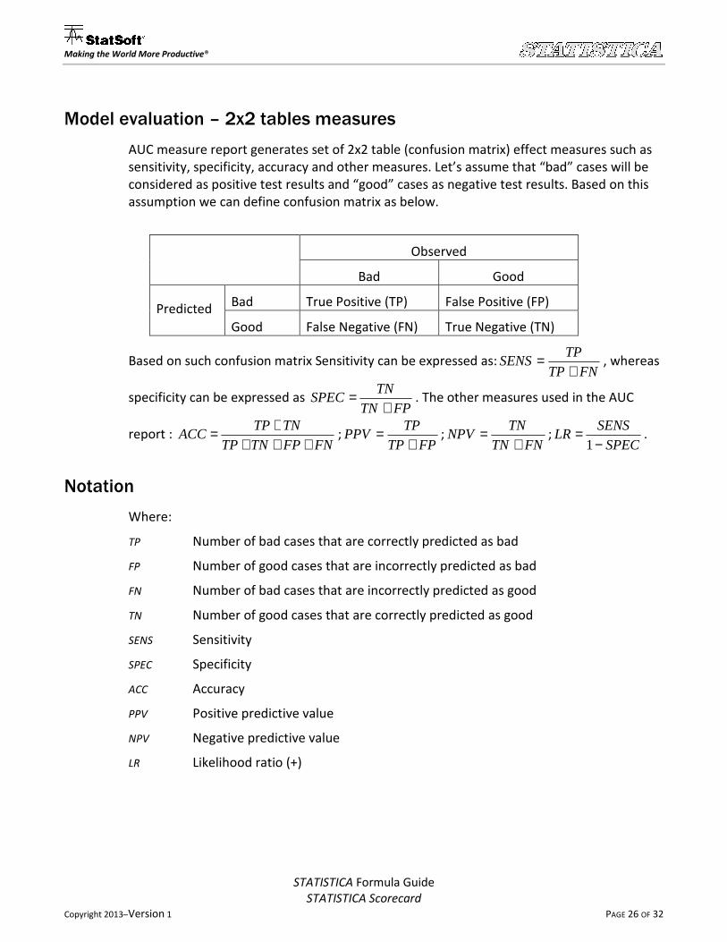
Model evaluation – 2x2 tables measures

AUC measure report generates set of 2x2 table (confusion matrix) effect measures such as

sensitivity, specificity, accuracy and other measures. Let’s assume that “bad” cases will be

considered as positive test results and “good” cases as negative test results. Based on this

assumption we can define confusion matrix as below.

Observed

Bad Good

Predicted Bad True Positive (TP) False Positive (FP)

Good False Negative (FN) True Negative (TN)

Based on such confusion matrix Sensitivity can be expressed as:FNTP

TPSENS

+= , whereas

specificity can be expressed as FPTN

TNSPEC

+= . The other measures used in the AUC

report : FNFPTNTP

TNTPACC

++++= ;

FPTP

TPPPV

+= ;

FNTN

TNNPV

+= ;

SPEC

SENSLR

−=

1.

Notation

Where:

TP Number of bad cases that are correctly predicted as bad

FP Number of good cases that are incorrectly predicted as bad

FN Number of bad cases that are incorrectly predicted as good

TN Number of good cases that are correctly predicted as good

SENS Sensitivity

SPEC Specificity

ACC Accuracy

PPV Positive predictive value

NPV Negative predictive value

LR Likelihood ratio (+)





Cut-off point selection

The Cut off point selection module is used to define the optimal value of scoring that separates

accepted and rejected applicants. You can extend the decision procedure by adding one or two

additional cut-off points (e.g., applicants with scores below 520 will be declined, applicants with scores

above 580 will be accepted, and applicants with scores between these values will be asked for

additional qualifying information). Cut-off points can be defined manually, based on a Receiver

Operating Characteristic (ROC) analysis for custom misclassifications costs and bad credit fraction.

(ROC analysis provides a measure of the predictive power of a model). Additionally, we can set optimal

cut-off points by simulating profit, associated with each cut-point level. Goodness of the selected cut-

off point can be assessed based on various reports. More information see : TUTORIAL Developing

Scorecards Using STATISTICA Scorecard [4].

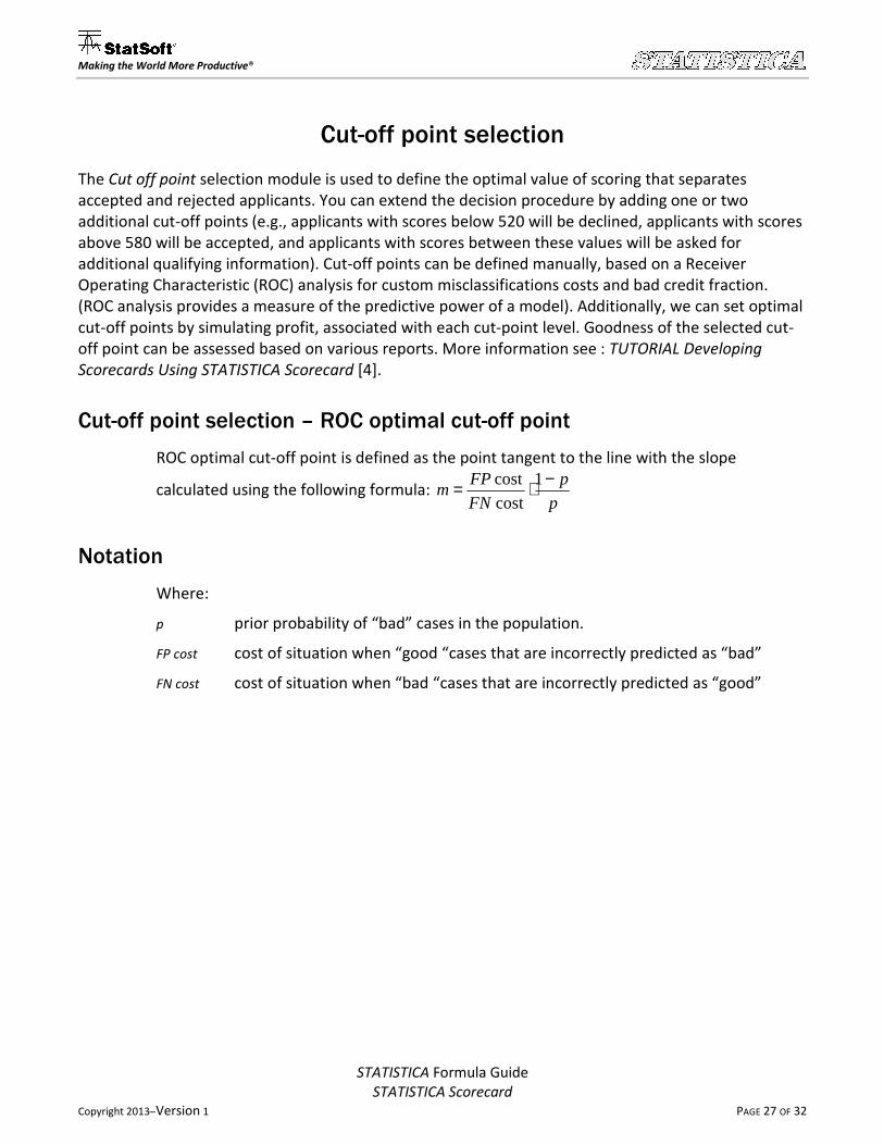
Cut-off point selection – ROC optimal cut-off point

ROC optimal cut-off point is defined as the point tangent to the line with the slope

calculated using the following formula: p

p

FN

FPm

−⋅= 1

cost

cost

Notation

Where:

p prior probability of “bad” cases in the population.

FP cost cost of situation when “good “cases that are incorrectly predicted as “bad”

FN cost cost of situation when “bad “cases that are incorrectly predicted as “good”





Score cases

The Score Cases module is used to score new cases using a selected model saved as an XML script. We

can calculate overall scoring, partial scorings for each variable, and probability of default from the

logistic regression model, adjusted by an a priori probability of default for the whole population

supplied by the user. For more information see TUTORIAL Developing Scorecards Using STATISTICA

Scorecard [4].

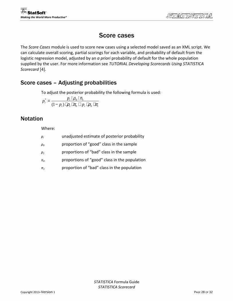
Score cases – Adjusting probabilities

To adjust the posterior probability the following formula is used:

1001

10*

)1( πρπρπρ

⋅⋅+⋅⋅−⋅⋅=

ii

ii pp

pp

Notation

Where:

pi unadjusted estimate of posterior probability

ρ0 proportion of “good” class in the sample

ρ1 proportions of “bad” class in the sample

π0 proportions of “good” class in the population

π1 proportion of “bad” class in the population





Calibration tests

The Calibration Tests module allows banks to test whether or not the forecast probability of default

(PD) has been the PD that has actually occurred. The Binomial Distribution and Normal Distribution

tests are included to test as appropriate the rating classes. The Austrian Supervision Criterion (see [5])

can be selected allowing STATISTICA to automatically choose the appropriate distribution test.

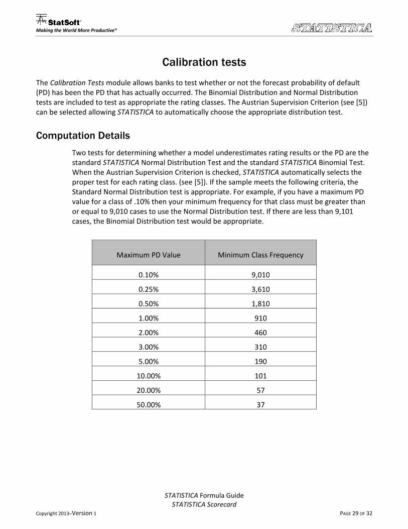
Computation Details

Two tests for determining whether a model underestimates rating results or the PD are the

standard STATISTICA Normal Distribution Test and the standard STATISTICA Binomial Test.

When the Austrian Supervision Criterion is checked, STATISTICA automatically selects the

proper test for each rating class. (see [5]). If the sample meets the following criteria, the

Standard Normal Distribution test is appropriate. For example, if you have a maximum PD

value for a class of .10% then your minimum frequency for that class must be greater than

or equal to 9,010 cases to use the Normal Distribution test. If there are less than 9,101

cases, the Binomial Distribution test would be appropriate.

Maximum PD Value Minimum Class Frequency

0.10% 9,010

0.25% 3,610

0.50% 1,810

1.00% 910

2.00% 460

3.00% 310

5.00% 190

10.00% 101

20.00% 57

50.00% 37





Population stability

The Population Stability module provides analytical tools for comparing two data sets (e.g., current and

historical data sets) in order to detect any significant changes in characteristic structure or applicant

population. Significant distortion in the current data set may provide a signal to re-estimate model

parameters. This module produces reports of population and characteristic stability with respective

graphs. For more information see TUTORIAL Developing Scorecards Using STATISTICA Scorecard [4].

Population stability

Population stability index measures the magnitude of the population shift between actual

and expected applicants. You can express this index using the following formula:

∑=

⋅−=k

i i

iii Expected

ActualExpectedActualstabilityPopulation

1

)ln()( .

Notation

Where:

k number of different score values or score ranges

Actuali percentage distribution of the total “Actual” cases in the ith

score value or score

range

Expectedi percentage distribution of the total “Expected” cases in the ith

score value or

score range





Characteristic stability

Characteristic stability index provides the information on shifts of distribution of variables

used for example in the scorecard building process. You can express this index using the

following formula: ∑=

⋅−=k

iiii scoreExpectedActualstabilitysticCharacteri

1

)( .

Notation

Where:

k number of categories of analyzed predictor

Actuali percentage distribution of the total “Actual” cases in the ith

category of

characteristic

Expectedi percentage distribution of the total “Expected” cases in the ith

category of

characteristic

scorei value of the score for the ith

category of characteristic





References

[1] Agresti, A. (2002). Categorical data analysis, 2nd ed. Hoboken, NJ: John Wiley & Sons.

[2] Hosmer, D, & Lemeshow, S. (2000). Applied logistic regression, 2nd ed. Hoboken, NJ: John Wiley &

Sons.

[3] Maddala, G. S. (2001) Introduction to Econometrics. 3rd

ed. John Wiley & Sons.

[4] Migut, G. Jakubowski, J. and Stout, D. (2013) TUTORIAL Developing Scorecards Using STATISTICA

Scorecard. StatSoft Polska/StatSoft Inc.

[5] Oesterreichishe Nationalbank. (2004). Guidelines on credit risk management: Rating models and

validation. Vienna, Austria: Oesterreichishe Nationalbank.

[6] Siddiqi, N. (2006). Credit Risk Scorecards: Developing and Implementing Intelligent Credit Scoring.

Hoboken, NJ: John Wiley & Sons.

[7] StatSoft, Inc. (2013). STATISTICA (data analysis software system), version 12. www.statsoft.com.

[8] Zweig, M. H., and Campbell, G. Receiver-operating characteristic (ROC) plots: a fundamental

evaluation tool in clinical medicine. Clinical chemistry 39.4 (1993): 561-577.

Documents

STATISTICA Scorecard Formula Guide guide/STATISTICA... · STATISTICA Scorecard is a comprehensive tool dedicated for developing, evaluating, and monitoring scorecard models. For more