Stationary and nonstationary generalized extreme value ...users.itia.ntua.gr/dpanag/B19.pdf · maxima in precipitation and discharge series, is fundamental for the design of engineering

Stationary and nonstationary generalized extremevalue modelling of extreme precipitation over amountainous area under climate changeD. Panagouliaa, P. Economoub and C. Caronic*

The generalized extreme value (GEV) distribution is often fitted to environmental time series of extreme values such asannual maxima of daily precipitation. We study two methodological issues here. First, we compare criteria for selecting thebestmodel among 16GEVmodels that allow nonstationary scale and location parameters. Simulation results showed that boththe corrected Akaike information criterion and Bayesian information criterion (BIC) always detected nonstationarity, but theBIC selected the correct model more often except in very small samples. Second, we examined confidence intervals (CIs) formodel parameters and other quantities such as the return levels that are usually required for hydrological and climatologicaltime series. Four bootstrap CIs—normal, percentile, basic and bias-corrected and accelerated—constructed by random-tresampling, fixed-t resampling and the parametric bootstrap methods were compared. CIs for parameters of the stationarymodel do not present major differences. CIs for the more extreme quantiles tend to become very wide for all bootstrapmethods. For nonstationary GEV models with linear time dependence of location or log-linear time dependence of scale, CIcoverage probabilities are reasonably accurate for the parameters. For the extreme percentiles, the bias-corrected andaccelerated method is best overall, and the fixed-t method also has good average coverage probabilities. A case study ispresented of annual maximum daily precipitation over the mountainous Mesochora catchment in Greece. Analysis ofhistorical data and data generated under two climate scenarios (control run and climate change) supported a stationaryGEV model reducing to the Gumbel distribution. Copyright © 2013 John Wiley & Sons, Ltd.

Keywords: GEV distribution; nonstationary models; model selection; bootstrap confidence intervals; maximum precipitation;climate change

1. INTRODUCTION: MODELLING ENVIRONMENTAL TIME SERIES WITH THEGENERALIZED EXTREME VALUE DISTRIBUTION

The generalized extreme value (GEV) distribution is widely employed for modelling extremes in the environmental sciences and many otherfields (see, for example, Reiss and Thomas, 2007, and references therein). It was introduced into meteorology by Jenkinson (1955) and isused extensively there to model extremes of natural phenomena such as precipitation (Gellens, 2002), temperature (Nogaj et al., 2007)and wind speed (Coles and Casson, 1999;Walshaw, 2000). The analysis of extremes in hydrometeorological data, such as the annual or monthlymaxima in precipitation and discharge series, is fundamental for the design of engineering structures (Maidment, 1993). In the case studypresented later in the paper, we examine annual extremes in historical precipitation data for a mountainous catchment in central-western Greece,as well as in simulated data obtained under different scenarios of climate change.

The GEV distribution combines into a single expression the three possible limiting distributions that arise from the limit theorem of Fisherand Tippett (1928) on extreme values or maxima in sample data. Its distribution function is

F x;μ;σ; ξð Þ ¼exp � 1þ ξ x� μð Þ

σ

� ��1ξ

8><>:

9>=>;; ξ≠0

exp � exp �x� μσ

h in o; ξ ¼ 0

8>>>>><>>>>>:

(1)

* Correspondence to: C. Caroni, Department of Mathematics, School of Applied Mathematical and Physical Sciences, National Technical University of Athens, 9 IroonPolytechniou, 157 80 Zografou, Athens, Greece. E-mail: [email protected]

a Department of Water Resources and Environmental Engineering, School of Civil Engineering, National Technical University of Athens, Athens, Greece

b Department of Civil Engineering, School of Engineering, University of Patras, Patras, Greece

c Department of Mathematics, School of Applied Mathematical and Physical Sciences, National Technical University of Athens, Athens, Greece

Environmetrics 2014; 25: 29–43 Copyright © 2013 John Wiley & Sons, Ltd.

Research Article Environmetrics

Received: 18 May 2012, Revised: 20 November 2013, Accepted: 25 November 2013, Published online in Wiley Online Library: 26 December 2013

(wileyonlinelibrary.com) DOI: 10.1002/env.2252

29

where μ ∈ℝ, σ> 0 and ξ ∈ℝ are the location, scale and shape parameters, respectively. The shape parameter ξ affects the support of the distri-bution. More specifically, when ξ =0, the GEV distribution is the Gumbel distribution with supportℝ; when ξ > 0, it corresponds to the Fréchetdistribution with support x≥μþ σ

ξ , and when ξ < 0, it corresponds to the (reversed) Weibull distribution families with support x≤μ� σξ .

The assumption of a series of independently and identically distributed data with constant properties through time (stationarity) may needto be modified to reflect the effect of long-term climate change on a phenomenon. For example, the series of maximum temperatures or max-imum precipitation in an area could show trends over a period. There is indeed mounting evidence that hydroclimatic extreme series are notstationary, owing to natural climate variability or anthropogenic climate change (Jain and Lall, 2001; Milly et al., 2008). Modellingnonstationarity within the framework of the GEV distribution requires extended models with covariate-dependent changes in at least oneof the distribution’s three parameters (Coles, 2001). This leads us to the nonstationary GEV distribution (El Adlouni et al., 2007; Leclercand Ouarda, 2007).

In the nonstationary case, the parameters of the model are expressed as a function of time t and possibly other covariates as well(Coles, 2001). We shall limit our investigation to the case of dependence only on time. The nonstationary GEV distribution can bedenoted as GEV (μ(t),σ(t), ξ(t)) with distribution function

F y;μ tð Þ;σ tð Þ; ξ tð Þð Þ ¼ exp � 1þ ξ tð Þ y� μ tð Þσ tð Þ

� ��1=ξ tð Þ( )(2)

Following Nogaj et al. (2007), El Adlouni et al. (2007) and Cannon (2010), we consider possible nonstationary behaviour of the locationμ and scale σ parameters but keep the shape parameter ξ constant.

More specifically, the following regression structures will be considered for location and scale parameters when (calendar) time is theexplanatory covariate

μ tð Þ ¼ μ0 þ μ1t þ μ2t2 þ μ3t

3

σ tð Þ ¼ exp σ0 þ σ1t þ σ2t2 þ σ3t3ð Þ (3)

allowing up to cubic dependence on time of both the location μ and scale σ parameters. We denote by GEVjk the model with timedependence of order j in the location parameter and order k in the scale parameter. For example, the stationary GEV distribution isGEV00, obtained when the location and scale parameters are both independent of time (μ1 =μ2 =μ3 = 0 and σ1 =σ2 =σ3 = 0), while theGEV21 nonstationary model assumes a quadratic trend (μ3 = 0) in location and a log-linear trend in scale (σ2 =σ3 = 0). Sixteen models ofvarying complexity may be defined in this way (four choices for each of j and k).

Nonstationarity could also be introduced by other approaches to modelling μ(t) and σ(t). Apart from the use of nonpolynomial functions oftime, the possibilities include fitting fractional polynomials (Royston and Altman, 1994) or a nonparametric approach (Chavez-Demoulinand Davison, 2005). It would be very demanding to investigate the performance of some of these methods in a simulation study. We havepreferred here to limit our investigation to fitting polynomials, which, as indicated in the previous texts, is an approach that is popular inapplications.

The specific aim of the present paper is to investigate two methodological aspects of the application of GEVjk models. One aspect is tocompare methods of selecting the best model from this set. The second is to compare methods of constructing confidence intervals for theparameters of the model and other quantities of interest. In the following section of the paper, we present the procedures for model fitting andselection. The third section compares the performances of the various criteria. The fourth section describes the quantification of the uncer-tainty in the estimates by bootstrap confidence intervals constructed by different methods, and the fifth, their comparison in a simulationstudy. A case study is presented in the sixth section, followed by conclusions in the final section.

2. STATISTICAL ISSUES

2.1. Model fitting and selection

The stationary and nonstationary GEV models may be fitted to a time series {y(ti) : ti ∈ T} where T= {t1, t2,…, tn} by maximizing the log-likelihood function

‘ ≡ log L ¼Xni¼1

� log σ tið Þð Þ � 1þ 1ξ

� �log 1þ ξ

y tið Þ � μ tið Þσ tið Þ

� �� 1þ ξ

y tið Þ � μ tið Þσ tið Þ

� ��1=ξ !

(4)

over the parameter space by numerical methods. This can be a challenging procedure, especially when high complexity is assumed for thelocation and scale parameters. It may facilitate the procedure if starting values are obtained by the L-moments method (Hosking, 1990). Themaximum likelihood method is sometimes criticized because it can give rise to physically unacceptable estimates; the Generalized MaximumLikelihood (GML) method of Martins and Stedinger (2000) avoids this by, in effect, constraining ξ within the range (�0.5, 0.5) (Katzet al., 2002). The restriction to ξ < 0.5 ensures that the variance of the GEV is finite. As seen in the succeeding texts, the unconstrainedmaximum likelihood estimates (MLE) of this parameter from our data fell well below this limit anyway.

All results reported in this paper were obtained in the R computing environment (R Development Core Team, 2011), using the gev.fitroutine in the ismev package (Coles and Stephenson, 2010) to fit stationary and nonstationary GEV distributions by maximum likelihood.

D. PANAGOULIA, P. ECONOMOU AND C. CARONIEnvironmetrics

wileyonlinelibrary.com/journal/environmetrics Copyright © 2013 John Wiley & Sons, Ltd. Environmetrics 2014; 25: 29–43

30

We followed the recommendation in the programme documentation to standardize covariates. Thus, the linear, quadratic and cubic terms intime were actually entered into the model as

x1i ¼ ti � m1

s1; x2i ¼ x21i � m2

s2; x3i ¼ x31i � m3

s3

where m1 and s1 are the mean and the standard deviation of the time covariate, respectively, and mj and sj (j= 2, 3) are the mean and the

standard deviation of the x j1i, respectively.

After fitting various candidate models to a given time series, we wish to select the best model. Any other GEVjk model must fit the databetter than GEV00 because adding more parameters to a model always leads to a better fit at the cost of increasing complexity. Both of themost widely used statistical criteria for model selection, the Akaike information criterion (AIC; Akaike, 1974) and the Bayesian informationcriterion (BIC; Schwarz, 1978) seek to balance these two opposing forces by penalizing the increasing number of parameters in the model.Because we will be examining small samples, we will use the corrected AIC (denoted AICc), which includes a small-sample correction, in

place of the basic AIC. If ‘ is the maximized value of the likelihood for a model containing p parameters and n is the sample size, the criteriaare defined as

AICc ¼ �2‘ þ 2pþ 2p pþ 1ð Þn� p� 1

(5)

(the third term is the correction) and

BIC ¼ �2‘ þ p log n: (6)

Bayesian information criterion generally penalizes more complex models more strongly than does the AIC. The preferred model amongthe candidate models is the one that minimizes the chosen criterion, although attention should also be paid to models with values close tothe minimum.

We may also use the likelihood ratio test to compare the goodness-of-fit of two hierarchically nested GEVjk models. If ‘0 denotes the

maximized log-likelihood of the simpler modelM0 and ‘1 the maximized log-likelihood of a more complex modelM1 that containsM0, then,

under standard conditions,�2 ‘0 � ‘1

� �asymptotically follows the chi-squared distribution with q d.f., where q is the number of additional

parameters in M1 compared with M0 (more details of model selection procedures can be found in Claeskens and Hjort (2008) and Burnhamand Anderson (2002), for example).

2.2. Quantifying uncertainty in estimates: confidence intervals

Confidence intervals for the parameters of the model, on the basis of the asymptotic normality of the MLEs, are given by

θ j ± za=2

ffiffiffiffiffiffiffiffiffiffiffiffiffiffiffiffiffiffiffiffiffiffiffiffiJn θ �1

� �jj

r(7)

where θ j is theMLE of the jth parameter, za/2 is the appropriate percentile point of the standard normal distribution for constructing a (1� a)100%

confidence interval and Jn θ �1

� �jjis the jth diagonal component of the observed information matrix based on a sample of n independent

observations.Because these confidence intervals rely on the asymptotic normality of the MLEs, they may not possess good coverage properties, espe-

cially for small sample sizes. For example, in the situation described in the succeeding texts in the simulation study, with n= 50, the 95%confidence intervals for parameters calculated by the aforementioned method all had estimated coverage proportions below the nominal0.95, as small as 0.90 in the case of the location parameter of the GEV01 model. Furthermore, we are usually not only interested in parameterestimates but also in quantiles of the GEV distribution. These are related to the return periods of extreme events: For example, the upper 1%point of the distribution of annual maxima has a 1/.01 = 100-year return period. It might be expected that estimates of extreme upper quantilesof the GEV distribution are far from being normally distributed even for moderate sample sizes. Therefore, we consider constructingconfidence intervals for all quantities of interest by bootstrap methods based on resampling techniques (Efron, 1979; Efron, 1987; Efronand Tibshirani, 1993; Mudelsee et al., 2003; Prudhomme et al., 2003). The basic idea of bootstrap methods is that a picture of the samplingdistribution for any statistic can be built up by resampling from the original data, and as a result, any characteristic of this statistic can beobtained from the bootstrap distribution. Kysely (2008) reported simulation results on the use of the bootstrap approach to constructconfidence intervals for estimates from GEV models in the stationary case only.

2.3. Bootstrap methods

There are three general approaches to bootstrapping models with a regression structure: random-t resampling (also called case resampling),fixed-t resampling (also called model-based resampling or residual resampling) and the parametric bootstrap (Freedman, 1981; Stine, 1985;Shao, 1996; Sahinler and Topuz, 2007). All three methods will be compared by simulations under different stationary and nonstationaryGEV models in the next section. In each approach, we take a large number R of resamples in an appropriate way. The model under study

GEV MODELLING OF EXTREME PRECIPITATION Environmetrics

Environmetrics 2014; 25: 29–43 Copyright © 2013 John Wiley & Sons, Ltd. wileyonlinelibrary.com/journal/environmetrics

31

is fitted to each one of these bootstrap samples, and the value of each statistic of interest is recorded in order to obtain its bootstrap distri-bution from these R replications.

In all the methods investigated in this study, we employ the full-sample bootstrap, that is, the resamples are always of the same size, n, asthe original sample. Much of the literature on bootstrapping for extremes refers to the m-out-of-n bootstrap, where m< n (e.g. Qi, 2008),which is necessary for the nonparametric estimation of quantiles. The need for that method does not arise here, where the extreme quantilesare estimated as functions of the estimated parameters of the fitted distribution.

2.3.1. Random-t resampling

In the random-t resampling approach, we simply take the R resamples from the observed data {y(ti) : ti ∈ T}, where T= {t1 ,t2,…, tn}, bysimple random sampling with replacement from the original sample.

2.3.2. Fixed-t resampling

In the fixed-t resampling approach, the covariates (in this study, time) are treated as fixed with respect to replication of the study. On the otherhand, the fitted values y tið Þ : ti∈Tf g obtained from the analysis of the original sample are treated as the expected values of the response forthe bootstrap sample. A bootstrap sample under these assumptions is obtained by resampling residuals from the original model and assigningthem to the fitted values v.

Cannon (2010) summarized the fixed-t resampling approach in the following steps: (i) fit the chosen GEVjk model to the data, obtaining

parameter estimates μ tið Þ, σ tið Þ and ξ ; (ii) compute the independently exponentially distributed Cox–Snell residuals from the fitted model

ε tið Þ ¼ 1þ ξy tið Þ � μ tið Þ

σ tið Þ� ��1=ξ

; i ¼ 1; 2;…; n (8)

(iii) resample the transformed residuals with replacement to form a bootstrapped set of residuals {ε(b)(ti) : i= 1, 2,…, n}; (iv) rescale thebootstrap residuals by inverting the transformation

y tið Þ ¼ μ tið Þ þ σ tið Þ ε bð Þ tið Þ �ξ � 1

ξ; i ¼ 1; 2;…; n (9)

(v) fit the GEVjkmodel to the bootstrap sample and store the statistics of interest; and (vi) repeat steps (iii)–(v) R times to obtain the bootstrapdistribution of each statistic of interest.

2.3.3. Parametric bootstrap

A different approach to obtaining a bootstrap distribution for each statistic of interest is to sample directly from the fitted distribution, insteadof resampling from the original data or from the transformed residuals. More specifically, n observations are generated under the GEVjkmodel with parameter values equal to the estimates obtained from the fit to the original data. In the case of a nonstationary GEVjk model,

in order to obtain a simulated bootstrap sample of size n, one observation is generated from the GEVjk μ tið Þ; σ tið Þ; ξ� �

distribution for

each ti ∈T, and the bootstrap sample is constructed from all n observations.

2.4. Types of bootstrap intervals

For each of the bootstrap approaches described in the previous subsection, four different confidence intervals can be constructed for eachstatistic of interest, on the basis of the normal approximation method, the percentile method, the basic bootstrap method and the bias-corrected and accelerated (BCa) method (Efron, 1987; DiCiccio and Efron, 1996). Each of these methods relies on different assumptions,and hence, they may have significantly different properties.

2.4.1. Normal approximation method

The normal approximation method assumes that the statistic of interest is normally distributed, at least approximately. Let θb be the mean of

the R bootstrap estimates θ jb; j ¼ 1; 2;…;R of θ and sd θb

� �their standard deviation. Under the normality assumption, a (1� a)100% bias-

corrected confidence interval for θ can be constructed using the formula

θ þ θ � θb� �

±za=2sd θb

� �

where θ is the estimate of θ based on the original data and θ � θb� �

is a bias correction computed using θb.

Because the GEV models described in Section 1 are fitted by maximum likelihood, the normality assumption is valid asymptotically.However, its accuracy in small samples is questionable, particularly for the quantiles and most especially for those corresponding to longperiod return levels.



32

2.4.2. Percentile method

The percentile method for constructing confidence intervals makes no assumption concerning the distribution of the statistic of interest. It isbased on the assumption that the distribution of the bootstrapped statistic approximates the true sampling distribution. Consequently, the

lower limit L of a (1� a)100% confidence interval for the statistic θ can be obtained as the a2R� �

ordered θb value and the upper limit U

as the R� a2R� �

ordered θb value, where [x] denotes the integer part of x.

2.4.3. Basic bootstrap method

The basic bootstrap method is similar to the percentile method, but it assumes that the distribution of the difference θ jb � θ between a

bootstrapped estimate and the MLE of θ approximates the distribution of the difference θ � θ between the MLE and the true value of θ.The confidence interval is constructed initially for θ � θ from the a

2R� �

and R� a2R� �

ordered values of θ jb � θ; j ¼ 1; 2…;R, and then, itis transformed in order to obtain the corresponding interval for θ.

The basic confidence intervals for θ can also be obtained directly from the percentile confidence interval (L,U) by the formula

2θ � U; 2θ � L� �

(10)

2.4.4. Bias-corrected and accelerated method

Bias-corrected and accelerated confidence intervals (Efron, 1987) may give a significant improvement compared with the other bootstrapintervals, although their accuracy can be erratic for small sample size. BCa confidence intervals are actually modifications of the percentileintervals, adjusted to have the correct bias and skewness.

A (1� a)100% BCa confidence interval for the statistic θ is given by

θ a1ð Þjb ; θ a2ð Þ

jb

� �(11)

where θ a1ð Þjb is the 100a1

th ordered value of the bootstrap estimates θ jb; j ¼ 1; 2…;R and θ a2ð Þjb is their 100a2

th ordered value; a1 and a2 are given by

a1 ¼ Φ z0 þz0 þ za=2

1� α z0 þ za=2

" #(12)

a2 ¼ Φ z0 þz0 þ z1�a=2

1� α z0 þ z1�a=2

" #

(13)

where Φ(�) is the standard normal distribution function. The bias-correction z0 for θ is

z0 ¼ Φ�1Ι θ jb � θ < 0� �

R

0@

1A (14)

where I is the indicator function. The acceleration α is one-sixth of the skewness of the set of the n jackknife or leaving-one-out estimates of θ,that is, one-sixth of the skewness of the estimates θ ið Þ; i ¼ 1; 2;…; n of θ where θ ið Þ is the estimate obtained when the ith observation is deletedfrom the original sample. Thus, the acceleration is computed from the formula

α ¼

Xni¼1

θ ið Þ � θ �ð Þ� �3

6Xni¼1

θ ið Þ � θ �ð Þ� �2 !3=2

(15)

where θ �ð Þ ¼

Xni¼1

θ ið Þ

n .



33

3. RESULTS OF SIMULATION STUDIES

3.1. Comparison of selection criteria

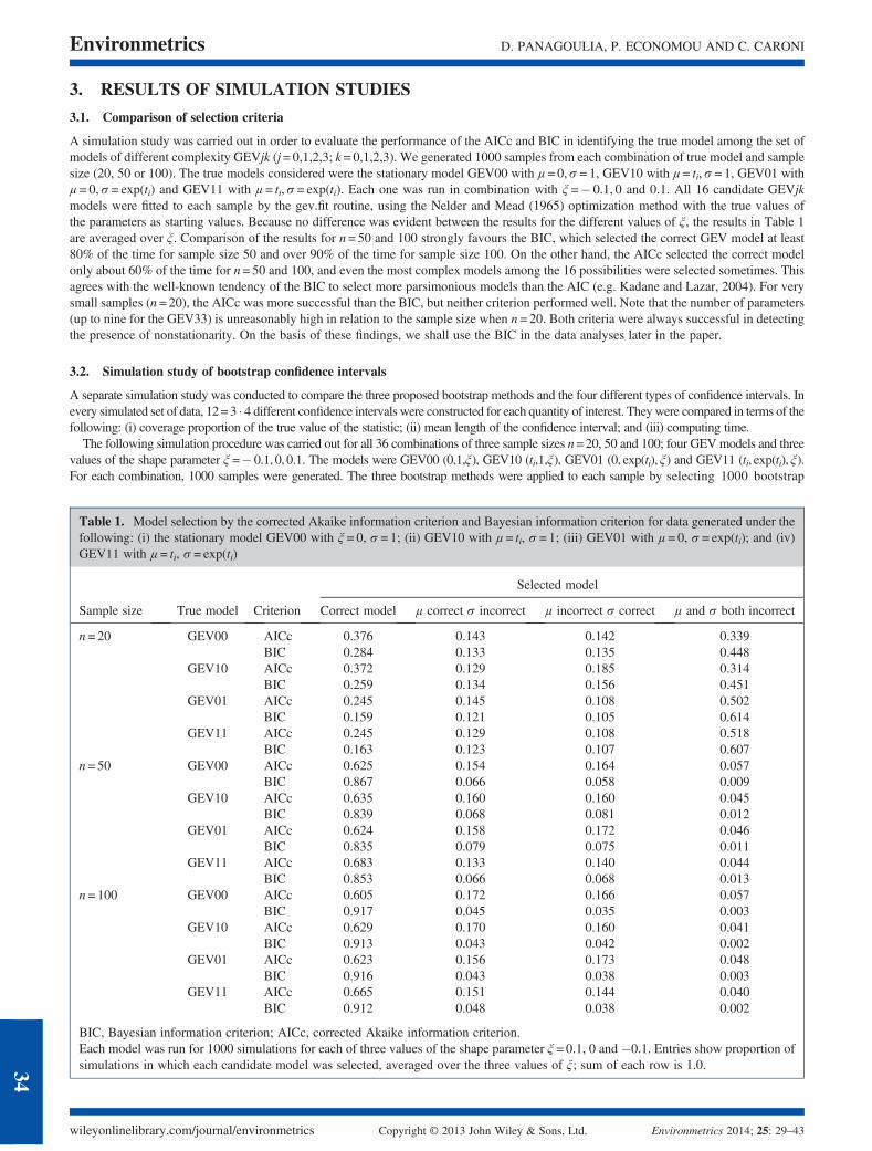
A simulation study was carried out in order to evaluate the performance of the AICc and BIC in identifying the true model among the set ofmodels of different complexity GEVjk (j= 0,1,2,3; k= 0,1,2,3). We generated 1000 samples from each combination of true model and samplesize (20, 50 or 100). The true models considered were the stationary model GEV00 with μ= 0,σ= 1, GEV10 with μ= ti,σ= 1, GEV01 withμ= 0,σ= exp(ti) and GEV11 with μ = ti,σ= exp(ti). Each one was run in combination with ξ =� 0.1, 0 and 0.1. All 16 candidate GEVjkmodels were fitted to each sample by the gev.fit routine, using the Nelder and Mead (1965) optimization method with the true values ofthe parameters as starting values. Because no difference was evident between the results for the different values of ξ, the results in Table 1are averaged over ξ. Comparison of the results for n= 50 and 100 strongly favours the BIC, which selected the correct GEV model at least80% of the time for sample size 50 and over 90% of the time for sample size 100. On the other hand, the AICc selected the correct modelonly about 60% of the time for n= 50 and 100, and even the most complex models among the 16 possibilities were selected sometimes. Thisagrees with the well-known tendency of the BIC to select more parsimonious models than the AIC (e.g. Kadane and Lazar, 2004). For verysmall samples (n= 20), the AICc was more successful than the BIC, but neither criterion performed well. Note that the number of parameters(up to nine for the GEV33) is unreasonably high in relation to the sample size when n= 20. Both criteria were always successful in detectingthe presence of nonstationarity. On the basis of these findings, we shall use the BIC in the data analyses later in the paper.

3.2. Simulation study of bootstrap confidence intervals

A separate simulation study was conducted to compare the three proposed bootstrap methods and the four different types of confidence intervals. Inevery simulated set of data, 12=3 � 4 different confidence intervals were constructed for each quantity of interest. Theywere compared in terms of thefollowing: (i) coverage proportion of the true value of the statistic; (ii) mean length of the confidence interval; and (iii) computing time.

The following simulation procedure was carried out for all 36 combinations of three sample sizes n=20, 50 and 100; four GEVmodels and threevalues of the shape parameter ξ =� 0.1, 0, 0.1. The models were GEV00 (0,1,ξ), GEV10 (ti,1,ξ), GEV01 (0, exp(ti), ξ) and GEV11 (ti, exp(ti), ξ).For each combination, 1000 samples were generated. The three bootstrap methods were applied to each sample by selecting 1000 bootstrap

Table 1. Model selection by the corrected Akaike information criterion and Bayesian information criterion for data generated under thefollowing: (i) the stationary model GEV00 with ξ = 0, σ= 1; (ii) GEV10 with μ = ti, σ= 1; (iii) GEV01 with μ = 0, σ= exp(ti); and (iv)GEV11 with μ = ti, σ= exp(ti)

Selected model

Sample size True model Criterion Correct model μ correct σ incorrect μ incorrect σ correct μ and σ both incorrect

n= 20 GEV00 AICc 0.376 0.143 0.142 0.339BIC 0.284 0.133 0.135 0.448

GEV10 AICc 0.372 0.129 0.185 0.314BIC 0.259 0.134 0.156 0.451

GEV01 AICc 0.245 0.145 0.108 0.502BIC 0.159 0.121 0.105 0.614

GEV11 AICc 0.245 0.129 0.108 0.518BIC 0.163 0.123 0.107 0.607

n= 50 GEV00 AICc 0.625 0.154 0.164 0.057BIC 0.867 0.066 0.058 0.009

GEV10 AICc 0.635 0.160 0.160 0.045BIC 0.839 0.068 0.081 0.012

GEV01 AICc 0.624 0.158 0.172 0.046BIC 0.835 0.079 0.075 0.011

GEV11 AICc 0.683 0.133 0.140 0.044BIC 0.853 0.066 0.068 0.013

n= 100 GEV00 AICc 0.605 0.172 0.166 0.057BIC 0.917 0.045 0.035 0.003

GEV10 AICc 0.629 0.170 0.160 0.041BIC 0.913 0.043 0.042 0.002

GEV01 AICc 0.623 0.156 0.173 0.048BIC 0.916 0.043 0.038 0.003

GEV11 AICc 0.665 0.151 0.144 0.040BIC 0.912 0.048 0.038 0.002

BIC, Bayesian information criterion; AICc, corrected Akaike information criterion.Each model was run for 1000 simulations for each of three values of the shape parameter ξ = 0.1, 0 and �0.1. Entries show proportion ofsimulations in which each candidate model was selected, averaged over the three values of ξ; sum of each row is 1.0.



34

samples each of size n, and for each bootstrap method, the four different bootstrap confidence intervals were computed for theparameters of the model and the quantiles corresponding to 2, 5, 10, 20, 50, 100 and 1000-year return levels (10 items in total).

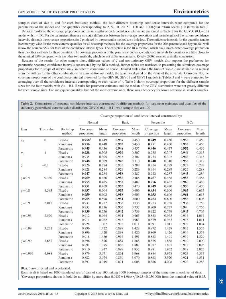
Detailed results on the coverage proportions and mean lengths of each confidence interval are presented in Table 2 for the GEV00 (0,1,�0.1)model with n=100. For the parameters, there are no major differences between the coverage proportions and mean lengths of the various confidenceintervals, although the coverage proportions for ξ produced by the percentile method are a little low. The confidence intervals for the quantiles tend tobecome very wide for the more extreme quantiles for all bootstrap methods, but the coverage proportions for the 90th percentile and beyond fall wellbelow the nominal 95% for three of the confidence interval types. The exception is the BCa method, which has a much better coverage proportionthan the other methods for these quantiles. The coverage proportion of the parametric bootstrap confidence intervals for quantiles is a little closer tothe nominal 95% compared with the other two methods, which do not differ substantially. Kysely (2008) reached a similar conclusion.

Because of the results for other sample sizes, different values of ξ and nonstationary GEV models also support the preference forparametric bootstrap confidence intervals constructed by the BCa method, further tables are restricted to presenting the simulated coverageproportions for this type of interval only, in order to economize on space. Detailed tables along the lines of Table 2 are available on requestfrom the authors for the other combinations. In a nonstationary model, the quantiles depend on the value of the covariate. Consequently, thecoverage proportions of the confidence interval presented for the GEV10, GEV01 and GEV11 models in Tables 3 and 4 were computed byaveraging over all the confidence intervals corresponding to each value of ti. Table 3 shows coverage proportions for the different samplesizes for the four models, with ξ =� 0.1. Results for parameter estimates and the median of the GEV distribution were not greatly differentbetween sample sizes. For subsequent quantiles, but not the most extreme ones, there was a tendency for lower coverage in smaller samples.

Table 2. Comparison of bootstrap confidence intervals constructed by different methods for parameter estimates and quantiles of thestationary generalized extreme value distribution GEV00 (0,1,�0.1), with sample size n= 100

Coverage proportion of confidence interval constructed by:

Normal Basic Percentile BCa

Item True value Bootstrapmethod

Coverageproportion

Meanlength

Coverageproportion

Meanlength

Coverageproportion

Meanlength

Coverageproportion

Meanlength

μ0 0 Fixed-t 0.9581 0.449 0.957 0.450 0.949 0.450 0.958 0.450Random-t 0.956 0.448 0.952 0.450 0.951 0.450 0.955 0.450Parametric 0.945 0.436 0.948 0.437 0.946 0.437 0.952 0.436

σ0 1 Fixed-t 0.938 0.305 0.939 0.307 0.935 0.307 0.944 0.313Random-t 0.935 0.305 0.935 0.307 0.934 0.307 0.946 0.313Parametric 0.948 0.309 0.945 0.310 0.940 0.310 0.955 0.312

ξ �0.1 Fixed-t 0.926 0.284 0.935 0.289 0.914 0.289 0.923 0.289Random-t 0.928 0.284 0.929 0.289 0.914 0.289 0.926 0.288Parametric 0.947 0.284 0.958 0.287 0.922 0.287 0.945 0.286

q= 0.5 0.360 Fixed-t 0.959 0.486 0.956 0.488 0.957 0.488 0.953 0.488Random-t 0.955 0.485 0.952 0.487 0.956 0.487 0.960 0.488Parametric 0.951 0.469 0.955 0.470 0.949 0.470 0.950 0.470







BCa, bias-corrected and accelerated.Each result is based on 1000 simulated sets of data of size 100, taking 1000 bootstrap samples of the same size in each set of data.1Coverage proportions shown in bold do not differ by more than 0.0135 = 1.96 ×√(0.95 × 0.05/1000) from the nominal value of 0.95.



35

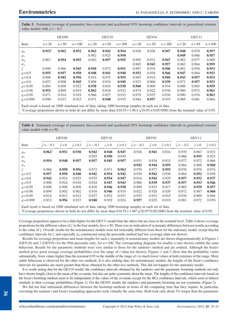
Coverage proportions appear to be a little higher for the GEV11 model than the others but are close to the nominal level. Table 4 shows coverageproportions for the different values of ξ in the four models, for n=50. There was no indication of systematic differences between results accordingto the value of ξ. Overall, results for the nonstationary models were not noticeably different from those for the stationary model, except that theconfidence intervals for ξ and especially σ0 constructed using the percentile method had low coverage (data not shown).

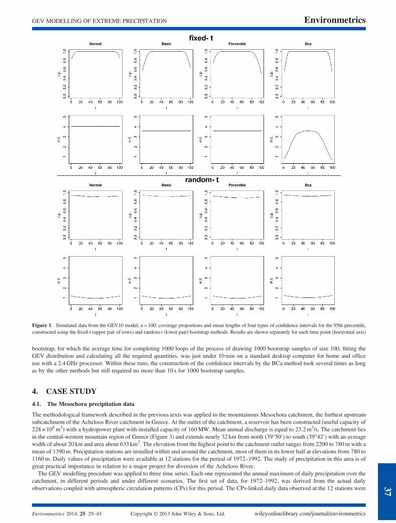
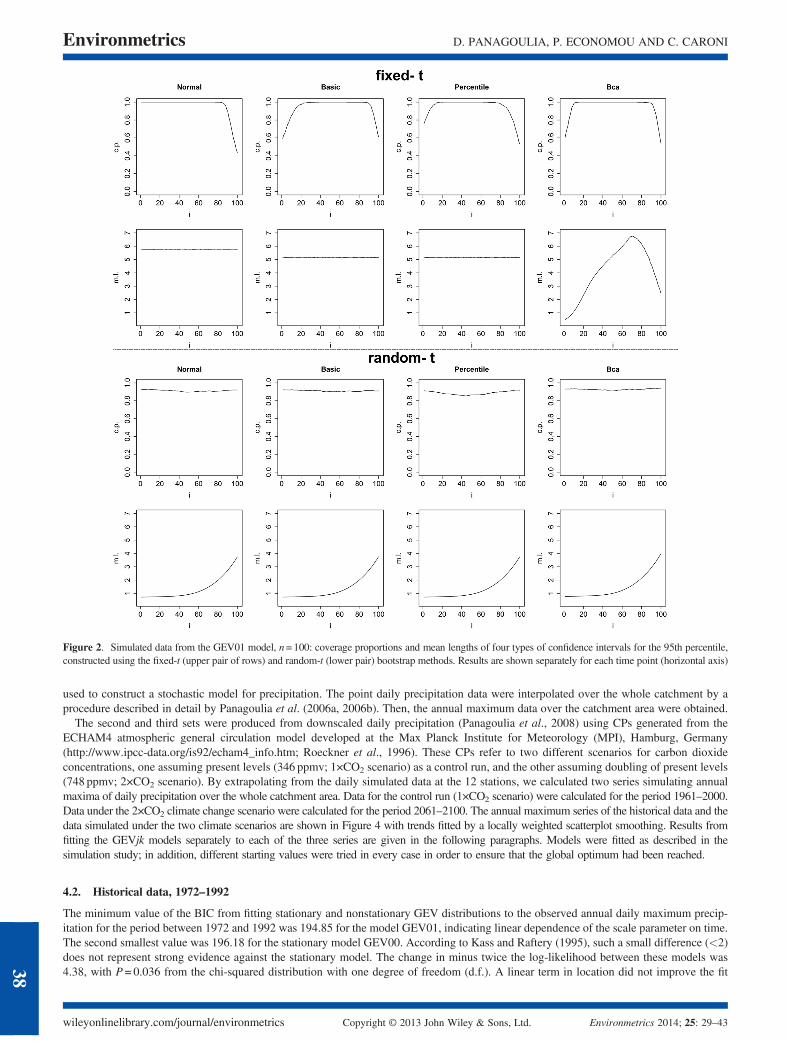
Results for coverage proportions and mean lengths for each ti separately in nonstationary models are shown diagrammatically in Figures 1(GEV10) and 2 (GEV01) for the 95th percentile only, for n= 100. The corresponding diagrams for smaller n (not shown) exhibit the samebehaviour. Results for the parametric methods were very similar to those for the random-t method and are omitted. Although the fixed-tmethod gives good average coverage probabilities over the range of t (data not shown), Figures 1 and 2 show that the probability variessubstantially, from values higher than the nominal 0.95 in the middle of the range of t to much lower values at both extremes of the range. Morestable behaviour is observed for the other two methods. It is also striking that, for nonstationary models, the lengths of the fixed-t confidenceintervals for quantiles are much greater than those obtained by the other two methods. This did not happen for the stationary model.

It is worth noting that for the GEV10 model, the confidence intervals obtained by the random-t and the parametric bootstrap methods not onlyhave shorter length, close to the mean of the covariate, but also are quite symmetric about the mean. The lengths of the confidence intervals based onthe fixed-t bootstrap method seem to be independent of the values of the covariate except for the BCa confidence intervals, which seem to behavesimilarly to their coverage probabilities (Figure 1). For the GEV01 model, the random-t and parametric bootstrap are not symmetric (Figure 2).

We did not find substantial differences between the bootstrap methods in terms of the computing time that they require. In particular,executing the random-t and fixed-t resampling approaches took virtually the same time. Both took only about 3% longer than the parametric

Table 3. Estimated coverage of parametric bias-corrected and accelerated 95% bootstrap confidence intervals in generalized extremevalue models with ξ =� 0.1

GEV00 GEV10 GEV01 GEV11

Item n= 20 n= 50 n= 100 n= 20 n= 50 n= 100 n= 20 n= 50 n= 100 n= 20 n= 50 n= 100

μ0 0.9531 0.962 0.952 0.962 0.942 0.954 0.936 0.926 0.947 0.948 0.970 0.957μ1 0.902 0.925 0.950 0.949 0.966 0.957σ0 0.967 0.954 0.955 0.982 0.957 0.955 0.995 0.931 0.947 0.982 0.977 0.969σ1 0.965 0.943 0.957 0.983 0.964 0.959ξ 0.998 0.966 0.945 0.958 0.972 0.951 0.987 0.976 0.946 0.981 0.976 0.953q= 0.5 0.955 0.957 0.950 0.948 0.941 0.948 0.952 0.930 0.946 0.947 0.964 0.953q= 0.8 0.906 0.942 0.956 0.916 0.935 0.955 0.905 0.914 0.944 0.943 0.957 0.953q= 0.9 0.857 0.908 0.945 0.898 0.924 0.949 0.923 0.906 0.939 0.972 0.957 0.953q= 0.95 0.884 0.898 0.922 0.938 0.916 0.938 0.960 0.909 0.934 0.986 0.965 0.959q= 0.98 0.952 0.899 0.919 0.962 0.918 0.932 0.974 0.922 0.930 0.990 0.972 0.961q= 0.99 0.971 0.914 0.918 0.966 0.927 0.932 0.979 0.935 0.930 0.990 0.976 0.963q= 0.999 0.990 0.933 0.923 0.971 0.948 0.935 0.984 0.957 0.935 0.989 0.981 0.964

Each result is based on 1000 simulated sets of data, taking 1000 bootstrap samples in each set of data.1Coverage proportions shown in bold do not differ by more than 0.0135 = 1.96 ×√(0.95 × 0.05/1000) from the nominal value of 0.95.

Table 4. Estimated coverage of parametric bias-corrected and accelerated 95% bootstrap confidence intervals in generalized extremevalue models with n= 50

GEV00 GEV10 GEV01 GEV11

Item ξ =� 0.1 ξ = 0 ξ = 0.1 ξ =� 0.1 ξ = 0 ξ = 0.1 ξ =� 0.1 ξ = 0 ξ = 0.1 ξ =� 0.1 ξ = 0 ξ = 0.1

μ0 0.9621 0.951 0.938 0.942 0.948 0.947 0.926 0.941 0.924 0.970 0.967 0.932μ1 0.925 0.950 0.930 0.966 0.955 0.925σ0 0.954 0.948 0.957 0.957 0.945 0.957 0.931 0.934 0.933 0.977 0.972 0.964σ1 0.943 0.944 0.959 0.964 0.968 0.960ξ 0.966 0.958 0.956 0.972 0.971 0.963 0.976 0.977 0.955 0.976 0.976 0.974q= 0.5 0.957 0.950 0.940 0.941 0.954 0.942 0.930 0.942 0.930 0.964 0.952 0.930q= 0.8 0.942 0.924 0.925 0.935 0.954 0.947 0.914 0.942 0.929 0.957 0.952 0.937q= 0.9 0.908 0.924 0.910 0.924 0.947 0.943 0.906 0.939 0.937 0.957 0.953 0.946q= 0.95 0.898 0.908 0.899 0.916 0.946 0.938 0.909 0.935 0.917 0.965 0.959 0.957q= 0.98 0.899 0.902 0.902 0.918 0.946 0.935 0.922 0.928 0.929 0.972 0.967 0.960q= 0.99 0.914 0.913 0.912 0.927 0.932 0.931 0.935 0.933 0.915 0.976 0.969 0.964q= 0.999 0.933 0.956 0.933 0.948 0.929 0.924 0.957 0.925 0.919 0.981 0.972 0.970

Each result is based on 1000 simulated sets of data, taking 1000 bootstrap samples in each set of data.1Coverage proportions shown in bold do not differ by more than 0.0135 = 1.96*√(0.95*0.05/1000) from the nominal value of 0.95.



36

bootstrap, for which the average time for completing 1000 loops of the process of drawing 1000 bootstrap samples of size 100, fitting theGEV distribution and calculating all the required quantities, was just under 10min on a standard desktop computer for home and officeuse with a 2.4GHz processor. Within these runs, the construction of the confidence intervals by the BCa method took several times as longas by the other methods but still required no more than 10 s for 1000 bootstrap samples.

4. CASE STUDY

4.1. The Mesochora precipitation data

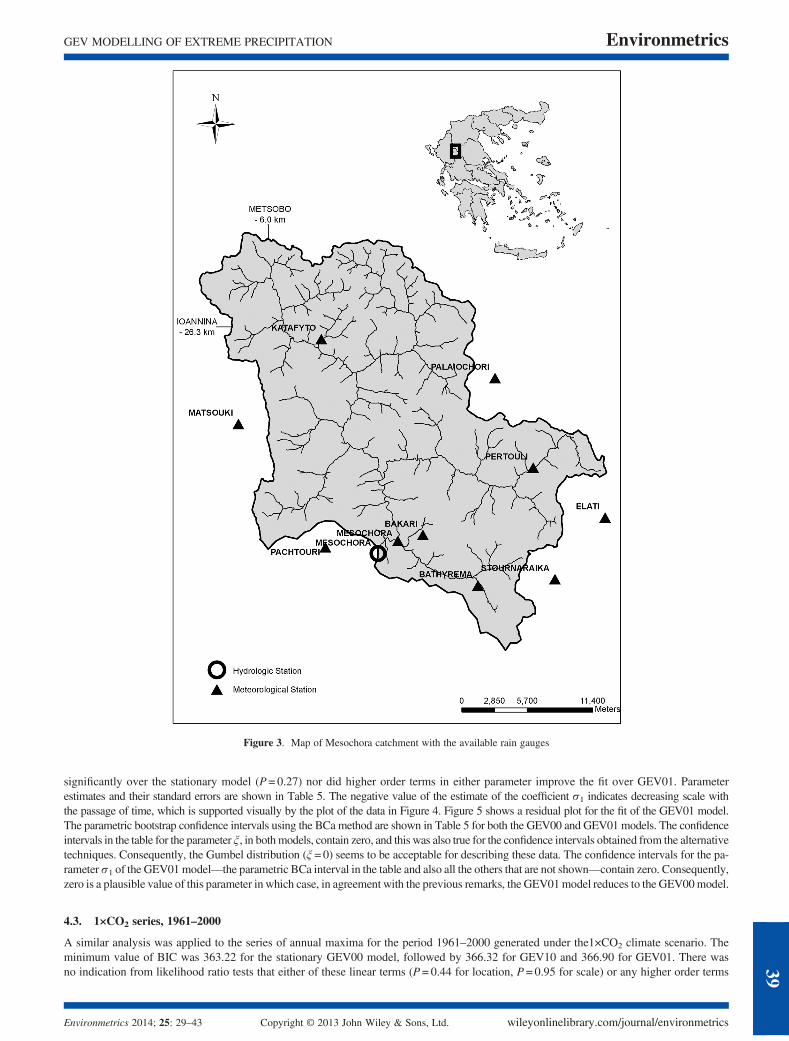
The methodological framework described in the previous texts was applied to the mountainous Mesochora catchment, the furthest upstreamsubcatchment of the Acheloos River catchment in Greece. At the outlet of the catchment, a reservoir has been constructed (useful capacity of228 × 106m3) with a hydropower plant with installed capacity of 160MW. Mean annual discharge is equal to 23.2m3/s. The catchment liesin the central-western mountain region of Greece (Figure 3) and extends nearly 32 km from north (39°50′) to south (39°42′) with an averagewidth of about 20 km and area about 633 km2. The elevation from the highest point to the catchment outlet ranges from 2200 to 780m with amean of 1390m. Precipitation stations are installed within and around the catchment, most of them in its lower half at elevations from 780 to1160m. Daily values of precipitation were available at 12 stations for the period of 1972–1992. The study of precipitation in this area is ofgreat practical importance in relation to a major project for diversion of the Acheloos River.

The GEV modelling procedure was applied to three time series. Each one represented the annual maximum of daily precipitation over thecatchment, in different periods and under different scenarios. The first set of data, for 1972–1992, was derived from the actual dailyobservations coupled with atmospheric circulation patterns (CPs) for this period. The CPs-linked daily data observed at the 12 stations were

Figure 1. Simulated data from the GEV10 model, n=100: coverage proportions and mean lengths of four types of confidence intervals for the 95th percentile,constructed using the fixed-t (upper pair of rows) and random-t (lower pair) bootstrap methods. Results are shown separately for each time point (horizontal axis)



37

used to construct a stochastic model for precipitation. The point daily precipitation data were interpolated over the whole catchment by aprocedure described in detail by Panagoulia et al. (2006a, 2006b). Then, the annual maximum data over the catchment area were obtained.

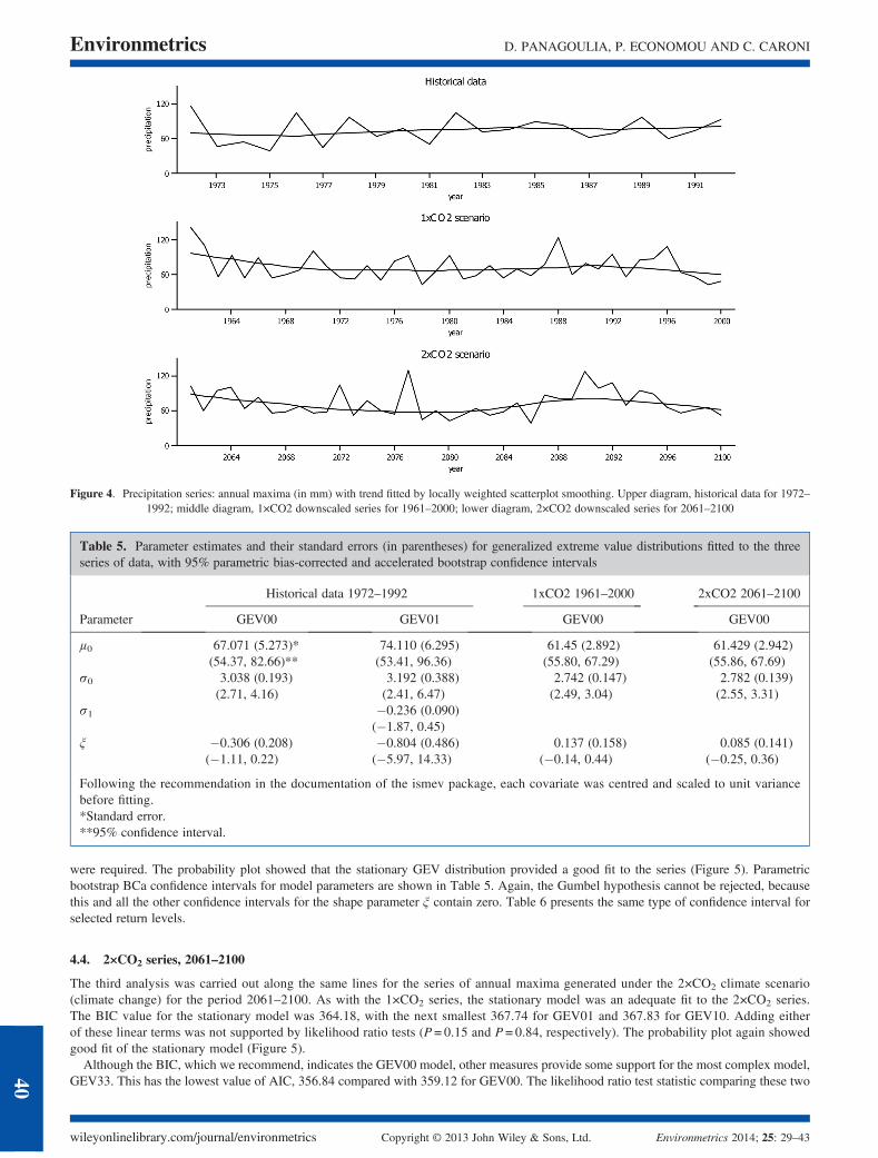
The second and third sets were produced from downscaled daily precipitation (Panagoulia et al., 2008) using CPs generated from theECHAM4 atmospheric general circulation model developed at the Max Planck Institute for Meteorology (MPI), Hamburg, Germany(http://www.ipcc-data.org/is92/echam4_info.htm; Roeckner et al., 1996). These CPs refer to two different scenarios for carbon dioxideconcentrations, one assuming present levels (346 ppmv; 1×CO2 scenario) as a control run, and the other assuming doubling of present levels(748 ppmv; 2×CO2 scenario). By extrapolating from the daily simulated data at the 12 stations, we calculated two series simulating annualmaxima of daily precipitation over the whole catchment area. Data for the control run (1×CO2 scenario) were calculated for the period 1961–2000.Data under the 2×CO2 climate change scenario were calculated for the period 2061–2100. The annual maximum series of the historical data and thedata simulated under the two climate scenarios are shown in Figure 4 with trends fitted by a locally weighted scatterplot smoothing. Results fromfitting the GEVjk models separately to each of the three series are given in the following paragraphs. Models were fitted as described in thesimulation study; in addition, different starting values were tried in every case in order to ensure that the global optimum had been reached.

4.2. Historical data, 1972–1992

The minimum value of the BIC from fitting stationary and nonstationary GEV distributions to the observed annual daily maximum precip-itation for the period between 1972 and 1992 was 194.85 for the model GEV01, indicating linear dependence of the scale parameter on time.The second smallest value was 196.18 for the stationary model GEV00. According to Kass and Raftery (1995), such a small difference (<2)does not represent strong evidence against the stationary model. The change in minus twice the log-likelihood between these models was4.38, with P= 0.036 from the chi-squared distribution with one degree of freedom (d.f.). A linear term in location did not improve the fit

Figure 2. Simulated data from the GEV01 model, n=100: coverage proportions and mean lengths of four types of confidence intervals for the 95th percentile,constructed using the fixed-t (upper pair of rows) and random-t (lower pair) bootstrap methods. Results are shown separately for each time point (horizontal axis)



38

http://www.ipcc-data.org/is92/echam4_info.htm

significantly over the stationary model (P= 0.27) nor did higher order terms in either parameter improve the fit over GEV01. Parameterestimates and their standard errors are shown in Table 5. The negative value of the estimate of the coefficient σ1 indicates decreasing scale withthe passage of time, which is supported visually by the plot of the data in Figure 4. Figure 5 shows a residual plot for the fit of the GEV01 model.The parametric bootstrap confidence intervals using the BCa method are shown in Table 5 for both the GEV00 and GEV01 models. The confidenceintervals in the table for the parameter ξ, in bothmodels, contain zero, and this was also true for the confidence intervals obtained from the alternativetechniques. Consequently, the Gumbel distribution (ξ =0) seems to be acceptable for describing these data. The confidence intervals for the pa-rameter σ1 of the GEV01model—the parametric BCa interval in the table and also all the others that are not shown—contain zero. Consequently,zero is a plausible value of this parameter in which case, in agreement with the previous remarks, the GEV01model reduces to the GEV00model.

4.3. 1×CO2 series, 1961–2000

A similar analysis was applied to the series of annual maxima for the period 1961–2000 generated under the1×CO2 climate scenario. Theminimum value of BIC was 363.22 for the stationary GEV00 model, followed by 366.32 for GEV10 and 366.90 for GEV01. There wasno indication from likelihood ratio tests that either of these linear terms (P= 0.44 for location, P = 0.95 for scale) or any higher order terms

Figure 3. Map of Mesochora catchment with the available rain gauges



39

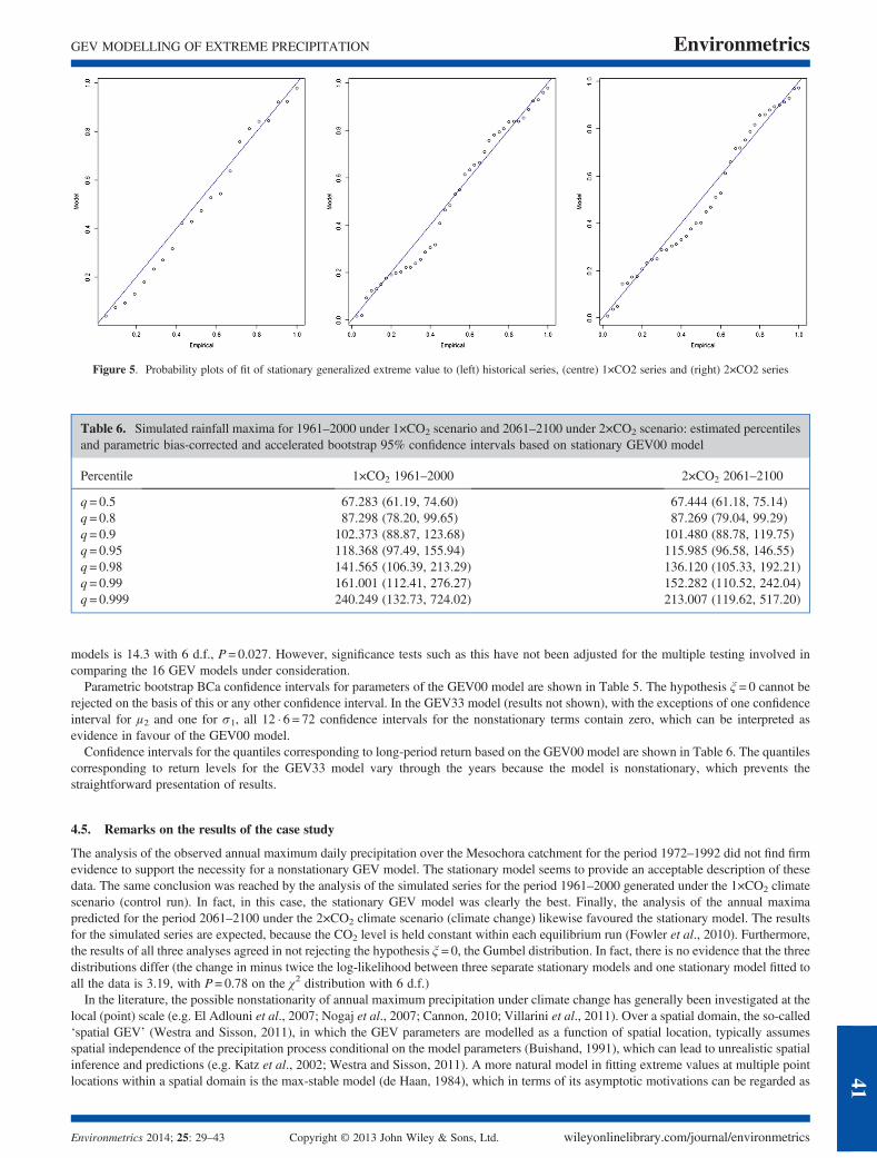
were required. The probability plot showed that the stationary GEV distribution provided a good fit to the series (Figure 5). Parametricbootstrap BCa confidence intervals for model parameters are shown in Table 5. Again, the Gumbel hypothesis cannot be rejected, becausethis and all the other confidence intervals for the shape parameter ξ contain zero. Table 6 presents the same type of confidence interval forselected return levels.

4.4. 2×CO2 series, 2061–2100

The third analysis was carried out along the same lines for the series of annual maxima generated under the 2×CO2 climate scenario(climate change) for the period 2061–2100. As with the 1×CO2 series, the stationary model was an adequate fit to the 2×CO2 series.The BIC value for the stationary model was 364.18, with the next smallest 367.74 for GEV01 and 367.83 for GEV10. Adding eitherof these linear terms was not supported by likelihood ratio tests (P = 0.15 and P = 0.84, respectively). The probability plot again showedgood fit of the stationary model (Figure 5).

Although the BIC, which we recommend, indicates the GEV00 model, other measures provide some support for the most complex model,GEV33. This has the lowest value of AIC, 356.84 compared with 359.12 for GEV00. The likelihood ratio test statistic comparing these two

Table 5. Parameter estimates and their standard errors (in parentheses) for generalized extreme value distributions fitted to the threeseries of data, with 95% parametric bias-corrected and accelerated bootstrap confidence intervals

Historical data 1972–1992 1xCO2 1961–2000 2xCO2 2061–2100

Parameter GEV00 GEV01 GEV00 GEV00

μ0 67.071 (5.273)* 74.110 (6.295) 61.45 (2.892) 61.429 (2.942)(54.37, 82.66)** (53.41, 96.36) (55.80, 67.29) (55.86, 67.69)

σ0 3.038 (0.193) 3.192 (0.388) 2.742 (0.147) 2.782 (0.139)(2.71, 4.16) (2.41, 6.47) (2.49, 3.04) (2.55, 3.31)

σ1 �0.236 (0.090)(�1.87, 0.45)

ξ �0.306 (0.208) �0.804 (0.486) 0.137 (0.158) 0.085 (0.141)(�1.11, 0.22) (�5.97, 14.33) (�0.14, 0.44) (�0.25, 0.36)

Following the recommendation in the documentation of the ismev package, each covariate was centred and scaled to unit variancebefore fitting.*Standard error.**95% confidence interval.

Figure 4. Precipitation series: annual maxima (in mm) with trend fitted by locally weighted scatterplot smoothing. Upper diagram, historical data for 1972–1992; middle diagram, 1×CO2 downscaled series for 1961–2000; lower diagram, 2×CO2 downscaled series for 2061–2100



40

models is 14.3 with 6 d.f., P= 0.027. However, significance tests such as this have not been adjusted for the multiple testing involved incomparing the 16 GEV models under consideration.

Parametric bootstrap BCa confidence intervals for parameters of the GEV00 model are shown in Table 5. The hypothesis ξ = 0 cannot berejected on the basis of this or any other confidence interval. In the GEV33 model (results not shown), with the exceptions of one confidenceinterval for μ2 and one for σ1, all 12 � 6 = 72 confidence intervals for the nonstationary terms contain zero, which can be interpreted asevidence in favour of the GEV00 model.

Confidence intervals for the quantiles corresponding to long-period return based on the GEV00 model are shown in Table 6. The quantilescorresponding to return levels for the GEV33 model vary through the years because the model is nonstationary, which prevents thestraightforward presentation of results.

4.5. Remarks on the results of the case study

The analysis of the observed annual maximum daily precipitation over the Mesochora catchment for the period 1972–1992 did not find firmevidence to support the necessity for a nonstationary GEV model. The stationary model seems to provide an acceptable description of thesedata. The same conclusion was reached by the analysis of the simulated series for the period 1961–2000 generated under the 1×CO2 climatescenario (control run). In fact, in this case, the stationary GEV model was clearly the best. Finally, the analysis of the annual maximapredicted for the period 2061–2100 under the 2×CO2 climate scenario (climate change) likewise favoured the stationary model. The resultsfor the simulated series are expected, because the CO2 level is held constant within each equilibrium run (Fowler et al., 2010). Furthermore,the results of all three analyses agreed in not rejecting the hypothesis ξ = 0, the Gumbel distribution. In fact, there is no evidence that the threedistributions differ (the change in minus twice the log-likelihood between three separate stationary models and one stationary model fitted toall the data is 3.19, with P= 0.78 on the χ2 distribution with 6 d.f.)

In the literature, the possible nonstationarity of annual maximum precipitation under climate change has generally been investigated at thelocal (point) scale (e.g. El Adlouni et al., 2007; Nogaj et al., 2007; Cannon, 2010; Villarini et al., 2011). Over a spatial domain, the so-called‘spatial GEV’ (Westra and Sisson, 2011), in which the GEV parameters are modelled as a function of spatial location, typically assumesspatial independence of the precipitation process conditional on the model parameters (Buishand, 1991), which can lead to unrealistic spatialinference and predictions (e.g. Katz et al., 2002; Westra and Sisson, 2011). A more natural model in fitting extreme values at multiple pointlocations within a spatial domain is the max-stable model (de Haan, 1984), which in terms of its asymptotic motivations can be regarded as

Table 6. Simulated rainfall maxima for 1961–2000 under 1×CO2 scenario and 2061–2100 under 2×CO2 scenario: estimated percentilesand parametric bias-corrected and accelerated bootstrap 95% confidence intervals based on stationary GEV00 model

Percentile 1×CO2 1961–2000 2×CO2 2061–2100

q= 0.5 67.283 (61.19, 74.60) 67.444 (61.18, 75.14)q= 0.8 87.298 (78.20, 99.65) 87.269 (79.04, 99.29)q= 0.9 102.373 (88.87, 123.68) 101.480 (88.78, 119.75)q= 0.95 118.368 (97.49, 155.94) 115.985 (96.58, 146.55)q= 0.98 141.565 (106.39, 213.29) 136.120 (105.33, 192.21)q= 0.99 161.001 (112.41, 276.27) 152.282 (110.52, 242.04)q= 0.999 240.249 (132.73, 724.02) 213.007 (119.62, 517.20)

Figure 5. Probability plots of fit of stationary generalized extreme value to (left) historical series, (centre) 1×CO2 series and (right) 2×CO2 series



41

the spatial analogue of the univariate GEV distribution (Westra and Sisson, 2011). The technique of pooling data from multiple locationsacross a spatial domain (e.g. Alexander et al., 2006; Fowler and Wilby, 2010) presents difficulties in terms of standardizing the data beforeaveraging and in developing the correct inferential method, particularly in the presence of spatial correlation between the original gaugeddata. Furthermore, local scale information is lost by pooling the data in this manner. In our case, we obtained the annual maximum precip-itation data over the area of the Mesochora catchment from point daily precipitation conditioned on atmospheric circulation by interpolation.This process may result in a smoothing effect on the extremes of precipitation. This is one possible reason for the finding of stationarity ratherthan nonstationarity in all three series. A second reason may be associated with the consideration of both wet and dry types of CPs indownscaled precipitation (Panagoulia et al., 2006a). In reality, only the wet types, usually occurring in winter, can cause the more extremevalues in precipitation (Mamassis and Koutsoyiannis, 1996). In conclusion, approaching climate change by examining the stationarity ornonstationarity of extreme precipitation (the latter supporting no climate change) comes up against the question, does the finding ofstationarity or nonstationarity of climate depend on the method employed? Many work towards answering this has been carried out by Linsand Cohn (2011), Koutsoyiannis (e.g. 2004, 2006, 2011) and Koutsoyiannis and Montanari (2007), who support the stationarity of climate.However, the true answer may be given in the future. Very long time series of extremes obtained from either gauged data or by more robustsimulation techniques at the appropriate spatial scale are required.

5. CONCLUSIONS

The possible nonstationarity of the GEV distribution fitted to annual maximum precipitation under climate change is a topic of activeinvestigation. It is important to have appropriate methods for selecting the best models. We investigated model selection within theGEVjk ( j = 0,1,2,3; k = 0,1,2,3) class of models with a time dependence of order j in the scale parameter and order k in the locationparameter, which is widely used for introducing nonstationarity. Our simulation results were based on fitting these models to data generated fromthe stationary GEV00 model and three nonstationary models: GEV10 (linear trend in location), GEV01 (log-linear trend in scale) and GEV11(linear trend in location and log-linear trend in scale). Our results clearly support the BIC for model selection, and we recommend its use. Oursecond aim in this study was to study how best to construct confidence intervals for items of interest arising from these GEV models. We exam-ined three bootstrapping approaches to constructing confidence intervals for parameters and quantiles: random-t resampling, fixed-t resamplingand the parametric bootstrap. Each approach was used in combination with the normal approximation method, percentile method, basic bootstrapmethod and BCa method for constructing confidence intervals. We found that all the confidence intervals for the stationary model parametershave similar coverage and mean length. For extreme quantiles, the BCa method produced confidence intervals with the best coverage. Thiswas also true for the nonstationary GEV10 and GEV01 models. Overall, our preferred type of confidence intervals is that produced by theparametric bootstrap method in combination with the BCa method.

REFERENCES

Akaike H. 1974. A new look at the statistical model identification. IEEE Transactions on Automatic Control 19: 716–723.Alexander LV, Zhang X, Peterson TC, Caesar J, Gleason B, Klein Tank A, Haylock M, Collins D, Trewin B, Rahimzadeh F, Tagipour A, Ambenje P,Rupa Kumar K, Revadekar J, Griffiths G, Vincent L, Stephenson DB, Burn J, Aguliar E, Brunet M, Taylor M, New M, Zhai P, Rusticucci M,Vazquez-Aguirre JL. 2006. Global observed changes in daily climate extremes of temperature and precipitation. Journal of Geophysical Research111: D05109. DOI: 10.1029/2005JD006290

Buishand AT. 1991. Extreme rainfall estimation by combining data from several sites. Hydrological Sciences Journal 36: 345–365.Burnham KP, Anderson DR. 2002. Model Selection andMultimodel Inference: A Practical Information-theoretic Approach (2nd ed.), Springer-Verlag: NewYork.Cannon AJ. 2010. A flexible nonlinear modelling framework for nonstationary generalized extreme value analysis in hydroclimatology. HydrologicalProcesses 24: 673–685.

Chavez-Demoulin V, Davison AC. 2005. Generalized additive modelling of sample extremes. Applied Statistics 54: 207–222.Claeskens G, Hjort NL. 2008. Model Selection and Model Averaging. Cambridge University Press: Cambridge.Coles GS. 2001. An Introduction to Statistical Modeling of Extreme Values. Springer: New York.Coles GS, Casson E. 1999. Extreme value modelling of hurricane wind speeds, Structural Safety 20: 283–296.Coles S, Stephenson A. 2010. ismev: an introduction to statistical modelling of extreme values. R package version 1.35. http://CRAN.R-project.org/package=ismev.

De Haan L. 1984. A spectral representation for max-stable processes. Annals of Probability 12: 1194–1204.DiCiccio TJ, Efron B. 1996. Bootstrap confidence intervals (with discussion). Statistical Science 11: 189–228.Efron B. 1979. Bootstrap methods: another look at the jackknife. Annals of Statistics 7: 1–26.Efron B. 1987. Better bootstrap confidence intervals (with discussion). Journal of the American Statistical Association 82: 171–200.Efron B, Tibshirani R. 1993. An Introduction to the Bootstrap. Chapman and Hall/CRC: Boca Raton, FL.El Adlouni S, Ouarda T, Zhang X, Roy R, Bobee B. 2007. Generalized maximum likelihood estimators for the non-stationary generalized extreme valuemodel. Water Resources Research 43: W03410. DOI: 10.1029/2005WR004545

Fisher RA, Tippett LHC. 1928. Limiting forms of the frequency distributions of the largest or smallest member of a sample. Proceedings of the CambridgePhilosophical Society 24: 180–190.

Fowler HJ, Wilby RL. 2010. Detecting changes in seasonal precipitation extremes using regional climate model projections: implications for managing fluvialflood risk. Water Resources Research 46: W03525. DOI: 10.1029/2008WR007636

Fowler HJ, Cooley D, Sain SR, Thurston M. 2010. Detecting change in UK extreme precipitation using results from the climateprediction.net BBC ClimateChange Experiment. Extremes 13: 241–267.

Freedman DA. 1981. Bootstrapping regression models. Annals of Statistics 9: 1218–1228.Gellens D. 2002. Combining regional approach and data extension procedure for assessing GEV distribution of extreme precipitation in Belgium. Journal ofHydrology 268: 113–126.

Hosking J. 1990. L-moments: analysis and estimation of distributions using linear combinations of order statistics. Journal of the Royal Statistical Society,Series B 52: 105–124.

Jain S, Lall U. 2001. Floods in a changing climate: does the past represent the future? Water Resources Research 37: 3193–3205.



42

http://CRAN.R-project.org/package=ismev

http://CRAN.R-project.org/package=ismev

Jenkinson AF. 1955. The frequency distribution of the annual maximum (or minimum) values of meteorological elements. Quarterly Journal of the RoyalMeteorological Society 81: 158–171.

Kadane JB, Lazar NA. 2004. Methods and criteria for model selection. Journal of the American Statistical Association 99: 279–290.Kass R, Raftery A. 1995. Bayes factors. Journal of the American Statistical Association 90: 773–795.Katz RW, Parlange MB, Naveau P. 2002. Statistics of extremes in hydrology. Advances in Water Resources 25: 1287–1304.Koutsoyiannis D. 2004. Statistics of extremes and estimation of extreme rainfall, 1. Theoretical investigation. Hydrological Sciences Journal 49: 575–690.Koutsoyiannis D. 2006. Non-stationarity versus scaling in hydrology. Journal of Hydrology 324: 239–354.Koutsoyiannis D. 2011. Hurst–Kolmogorov dynamics and uncertainty. Journal of the American Water Resources Association 47: 481–495.Koutsoyiannis D, Montanari A. 2007. Statistical analysis of hydroclimatic time series. Uncertainty and insights. Water Resources Research 43: W05429. DOI:

10.1029/2006WR005592.Kysely J. 2008. A cautionary note on the use of nonparametric bootstrap for estimating uncertainties in extreme-value models. Journal of Applied Meteorology

and Climatology 47: 3236–3251.Leclerc M, Ouarda T. 2007. Non-stationary regional flood frequency analysis at ungauged sites. Journal of Hydrology 343: 254–265.Lins HF, Cohn TA. 2011. Stationarity: wanted dead or alive? Journal of the American Water Resources Association 47: 475–480.Maidment DR. 1993. Handbook of Hydrology. McGraw-Hill: New York.Mamassis N, Koutsoyiannis D. 1996. Influence of atmospheric circulation types on space-time distribution of intense rainfall. Journal of Geophysical Research

101(D21): 26,267–26,276.Martins ES, Stedinger JR. 2000. Generalized maximum-likelihood generalized extreme-value quantile estimators for hydrologic data. Water Resources

Research 36: 737–744.Milly PCD, Betancourt J, Falkenmark M, Hirsch M, Kundzewicz ZW, Lettenmaier DP, Stouffer RJ. 2008. Stationarity is dead: whither water management?

Science 319: 573–574.Mudelsee M, Börngen M, Tetzlaff G, Grünewald U. 2003. No upward trends in the occurrence of extreme floods in central Europe. Nature 425: 166–169.Nelder JA, Mead R. 1965. A simplex algorithm for function minimization. Computer Journal 7: 308–313.Nogaj M, Parey S, Dacunha-Castelle D. 2007. Non-stationary extreme models and a climatic application. Nonlinear Processes in Geophysics 14: 305–316.Panagoulia D, Grammatikogiannis A, Bárdossy A. 2006a. An automated classification method of daily circulation patterns for surface climate data downscal-

ing based on optimised fuzzy rules. Global Nest Journal 8: 218–223.Panagoulia D, Bárdossy A, Lourmas G. 2006b. Diagnostic statistics of daily rainfall variability in an evolving climate. Advances in Geosciences 7: 349–354.Panagoulia D, Bárdossy A, Lourmas G. 2008. Multivariate stochastic downscaling model for generating precipitation and temperature of climate change based

on atmospheric circulation atmospheric circulation. Global Nest Journal 10: 263–272.Prudhomme C, Jakob D, Svensson C. 2003. Uncertainty and climate change impact on the flood regime of small UK catchments. Journal of Hydrology 277: 1–23.Qi Y. 2008. Bootstrap and empirical likelihood methods in extremes. Extremes 11: 81–97.R Development Core Team. 2011. R: a language and environment for statistical computing. R Foundation for Statistical Computing, Vienna, Austria. URL

http://www.R-project.org/Reiss RD, Thomas M. 2007. Statistical Analysis of Extreme Values with Applications to Insurance, Finance, Hydrology and Other Fields (3rd ed.),

Birkhauser: Basel.Roeckner E, Arpe K, Bengtsson L, Christoph M, Claussen M, Dümenil L, Esch M, Giorgetta M, Schlese U, Schulzweida U. 1996. The atmospheric general

circulation model ECHAM-4: model description and simulation of present-day climate. Report No. 218. Max-Planck Institute for Meteorology, Hamburg,Germany, 90pp.

Royston P, Altman D. 1994. Regression using fractional polynomials of continuous covariates: parsimonious parametric modelling (with discussion). AppliedStatistics 43: 429–467.

Sahinler S, Topuz D. 2007. Bootstrap and jackknife resampling algorithms for estimation of regression parameters. Journal of Applied Quantitative Methods 2:188–199.

Schwarz GE. 1978. Estimating the dimension of a model. Annals of Statistics 6: 461–464.Shao J. 1996. Bootstrap model selection. Journal of the American Statistical Association 91: 655–665.Stine R. 1985. Bootstrap prediction intervals for regression. Journal of the American Statistical Association 80: 1026–1031.Villarini G, Smith J, Baeck ML, Vitolo R, Stephenson D, Krajewski W. 2011. On the frequency of heavy rainfall for the Midwest of the United States. Journal

of Hydrology 400: 103–120.Walshaw D. 2000. Modelling extreme wind speeds in regions prone to hurricanes. Applied Statistics 49: 51–62.Westra S, Sisson S. 2011. Detection of non-stationarity in precipitation extremes using max-stable process model. Journal of Hydrology 406: 119–128.



43

http://www.R-project.org/

Documents

Stationary and nonstationary generalized extreme value ...users.itia.ntua.gr/dpanag/B19.pdf · maxima in precipitation and discharge series, is fundamental for the design of engineering