Embed Size (px)
Citation preview

COMPLEX – State of the Art Review of Climate-Energy-Economic Modeling Approaches
COMPLEX Report D5.1 i
STATE OF THE ART REVIEW OF CLIMATE-ENERGY-ECONOMIC MODELING APPROACHES
Date Report Number
15.09.2013 D5.1
VERSION NUMBER: Main Authors:
0_1 Overview of Climate Impact Assesmnt Modeling: Iñigo Capellán-Pérez, BC3 Iñaki Arto, BC3 Anil Markandya, BC3 Mikel González-Eguinob, BC3 Overview of Agent-based modeling: Tatiana Flatova, UoT Felix Pinouche, UoT Overview of CGE modeling: Mohammed Chahim Overview of System Dynamics modeling: Dmitry V. Kovalevsky, NIERSC Klaus Hasselmann, MPG
DIFFUSION LEVEL – RU PU
PU PUBLIC
RIP RESTRICTED INTERNAL AND PARTNERS
RI RESTRICTED INTERNAL
CO CONFIDENTIAL
Coordinator: Saeed Moghayer, TNO

COMPLEX – State of the Art Review of Climate-Energy-Economic Modeling Approaches
COMPLEX Report D5.1 ii
INFORMATION ON THE DOCUMENT
Title State of the Art Review of Climate-Energy-Economic Modeling
Approaches
Authors
Overview of Climate Impact Assesmnt Modeling:
Iñigo Capellán-Pérez, BC3
Iñaki Arto, BC3
Anil Markandya, BC3
Mikel González-Eguinob, BC3
Overview of Agent-based modeling:
Tatiana Filatova, UoT
Felix Pinouche, UoT
Overview of CGE modeling:
Mohammed Chahim
Overview of System Dynamics modeling:
Dmitry V. Kovalevsky, NIERSC
Klaus Hasselmann, MPG
Co-author Saeed Moghayer, TNO
DEVELOPMENT OF THE DOCUMENT
Date Version Prepared by Institution Approved by Note
15.09.13 0.1

COMPLEX – State of the Art Review of Climate-Energy-Economic Modeling Approaches
COMPLEX Report D5.1 iii
INDEX
1. Introduction ...................................................................................................................... 4
2. Overview of Climate Integrated Assessment Modeling ................................................... 5 2.1 Introduction ......................................................................................................... 5 2.2 IAM review.......................................................................................................... 6
2.2.1 General review aspects ........................................................................... 7 2.2.2 Specific review: the discount rate and quality concerns ...................... 19
2.3 Classification of climate IA models .................................................................. 20 2.4 Discussion on the state of the art of IAM .......................................................... 23 Appendix A: Climate IA models .................................................................................... 25
3. Overview of Environmental Computational General Equilibrium Models .................... 27 3.1 Introduction ....................................................................................................... 27 3.2 Classification of CGE models ........................................................................... 28 3.3 Environmental CGE review ............................................................................... 29
3.3.1 General review aspects ......................................................................... 29 3.3.2 Specific review of a number of existing environmental CGE models . 32
3.4 Discussion .......................................................................................................... 41 Appendix B: Environnemental CGE models ................................................................. 42
4. Overview of Climate-Energy-Economic Agent-Base Modeling.................................... 43 4.1 Introduction ....................................................................................................... 43 4.2 Climate-Energy-Economic ABM review .......................................................... 44
4.2.1 General review aspects ......................................................................... 45 4.2.2 ABM specific review aspects ............................................................... 54
4.3 Summary of reviewed ABMs characteristics .................................................... 56
5. Overview of Climate-Energy-Economic System Dynamic Modeling ........................... 73 5.1 Introduction ....................................................................................................... 73 5.2 Climate-Energy-Economic SD review .............................................................. 73
5.2.1 Review of general criteria as applied to SD modeling ......................... 73 5.2.2 Review of approach-specific criteria as applied to SD modeling ........ 75
5.3 Discussion .......................................................................................................... 75
6. Summary ........................................................................................................................ 76
References ................................................................................................................................... 79

COMPLEX – State of the Art Review of Climate-Energy-Economic Modeling Approaches
4
1. Introduction
Climate-energy-economy models are a fundamental tool to evaluate mitigation strategies and assess their
economic costs. These models include a representation of socio-economic processes, such as economic
growth and the dynamics of consumption and investment. Energy is usually regarded as a production factor,
alongside capital and labor. Energy, in turn, is generated through conversion processes from primary energy
sources, such as fossil fuels, uranium, wind, solar radiation, hydropower, or biomass. To link energy use to
climate impacts, carbon emissions from the combustion of fossil fuels are computed and their effects on
atmospheric concentrations and temperatures are assessed using a coupled climate module. To account for the
fact that climate change is a global and long-term challenge, climate-energy-economy models are required to
represent the entire world economy and carry out simulations over the period of a century.
Different models may generate very different sets of scenarios, depending on the view of the world they
represent regarding e. g. assumptions on future technological developments in the energy sector, inertia in the
deployment of new technologies, and how economic agents form expectations. Some models surprisingly
conclude – in direct contradiction of the urgency expressed in the scientific literature – that rapid,
comprehensive emissions abatement is both economically unsound and unnecessary. And some models seem
to ignore (and implicitly endorse the continuation of) gross regional imbalances of both emissions and
income.
In case of most of the existing climate-energy-economy models, their results are driven by conjectures and
assumptions that do not rest on empirical data and often cannot be tested against data until after the fact.
Better-informed climate policy decisions might be possible if the effects of controversial economic
assumptions and judgments were visible, and were subjected to sensitivity analyses and validation.
Existing climate-energy-economy models fully rely on the neoclassical abstractions of narrowly rational
individuals, fully optimizing firms, and perfectly functioning markets have attractive mathematical properties,
but as scientific hypotheses they do not withstand decisive tests against the evidence. It should come as no
surprise that the forecasts derived from such inadequate models are uncertain and unreliable.
Successful modeling “must reflect what people and organizations actually do” (Laitner et al., 2000).
Unfortunately, the majority of models appear to mischaracterize the behavior of economic agents with
“unsubstantiated assumptions about the characteristics of consumers and firms” (ibid., p. 1). Among other
things, the models depict the behavior of all consumers and businesses as a group, distilling the literally
millions of decisions made by millions of individuals into a few “representative agents” that do not interact
with each other, except very indirectly and only in response to price signals.
The models have improved over the years, including expanded treatment of externalities, technological
innovation, and regional disaggregation. But there is still tremendous scope for further improvement,
including the difficulty to represent pervasive technological developments, the difficulty to represent non-
linearities, thresholds and irreversibility, and the insufficiently developed representation of economic sectors
with a significant potential for mitigation and resource efficiency. COMPLEX aims to improve the present
state-of-the-art in Climate-Energy-Economy impact assessment modeling by tackling these relevant
limitations.
In order to that Working Package 5 of COMPLEX project develops a system of integrated complex models
combining insights from different field of research and modeling approaches: integrated assessment modeling
(IAM), System Dynamic (SD) models, Computational General Equilibrium (CGE) modeling and agent-base
modeling (ABM). The main emphasizes are on utilizing the non-linear climate responses and regime-shifts of
economic-ecological systems, modeling non-linear processes of diffusion and pervasive technical change and
its implication, and representation of economic sectors with a significant potential for mitigation and resource
efficiency.

COMPLEX – State of the Art Review of Climate-Energy-Economic Modeling Approaches
5
This report identifies a set of modeling tools that have been applied to relevant socio-economic aspects of the
assessments of the impact of climate change and relevant energy and environmental measures and policies.
The focus here is on the modeling approaches that will be utilized in the WP5 system of economic-energy-
environmental models: the review covers both more traditional modeling techniques such as Computational
General Equilibrium (CGE) model and Integrated Impact Assessment model (IAM) as well as more recent
innovative approaches to model complex systems including agent-based modeling (ABM) and system
dynamics SD) modeling.
The review is conducted based on some general and modeling approach specific criteria. The general review
criteria are designed in a broad sense, however, emphasizes more on the relevant aspects of COMPLEX
project and specifically WP5 objectives, which were discussed above.
2. Overview of Climate Integrated Assessment Modeling
2.1 Introduction
Integrated Assessment Modeling (IAM) is an interdisciplinary process which combines, explains, and
communicates knowledge from a range of disciplines in order to weigh up an entire chain of causes and
effects. Integrated Assessment (IA) is neither a new concept nor an activity restricted to Climate Change,
although the proliferation of models in the last two decades is due mainly to its application to climatic
research (Tol, 2006). The central element in IAM of climate change is the climate cantered economy-energy-
environment (E3) IA model, although the whole IAM process should not be reduced to the model, since IAM
includes problem definition, formulation of the policy questions, and interpretation and communication of the
results (IPCC SRES, 2000; Kriegler et al., 2012; MEA, 2005; Schwartz, 2003; Tol, 2006; Weyant et al.,
1995).
The development of IA models consists of the construction of dynamic models that integrate multiple
disciplines (economy, natural sciences, engineering, etc.), trying to capture interactions between human and
natural systems, and with the aim of providing useful information for policy making. The relationships
analysed by IA models tend to be very complex, dynamic and often highly nonlinear. Nevertheless, IA models
should not be identified as an oracle: the results they provide depend on the assumptions and methods
considered for their construction, and are subject to high scientific and social-response uncertainties. One
approach for dealing with uncertainty is through developing scenarios that provide plausible descriptions of
how the future might unfold in different socioeconomic, technological and environmental conditions. In this
sense, the interpretation of the results is in tight relation with the set of hypothesis and conditions considered.
The combination of the multidisciplinary and the scenario approaches allows IA models to offer a strategic
and comprehensive view of the whole phenomenon studied and its uncertainties.
IAM applied to climate change is typically oriented to inform policy-makers on the feasibility and costs of
meeting alternative climate stabilization targets under a range of salient long-term uncertainties. Since climate
change is an anthropogenic phenomenon characterised by complex feedbacks between socioeconomic an
ecological systems, IA models attempt to integrate the human (economic, behavioural, institutional, lifestyle,
etc.) and biophysical (land-use, climate, ecosystems, etc.) spheres. Different climate mitigation pathways are
then explored assuming that the climate problem will be internalized by the economy in the future. IA models
are generally focused on “insights about the nature and structure of the climate problem, about what matters,
and about what we still need to learn” (Morgan and Dowlatabadi, 1996, p. 337) and face questions such as:
Which set of policies and technologies would be able to mitigate the adverse effects of climate
change at a minimum cost?”
“What are the costs of non-action as well as mitigation/adaptation opportunities?”
“What are the links and feedbacks between the different human sectors (socioeconomic,
agriculture, forestry, energy, etc.) and between them and the natural subsystems (climate,
ecosystems, coastal zones, etc.)?”

COMPLEX – State of the Art Review of Climate-Energy-Economic Modeling Approaches
6
Etc.
Dozens of climatic E3 currently exist: a review in 1995 already identified more than 30 models (Weyant et al.,
1995); nowadays most of them continue to be developed and many more have been created (e.g. (Stanton et
al., 2009; Tol, 2006)). Appendix A includes a selection of 26 representative IA models currently used in
climate assessment, sorted by chronologically order of creation. Model diversity is directly related with
critical uncertainties in climate science and analysis methodologies. Thus a multi-model approach is usually
adopted at the policy level (e.g. IPCC assessments).
Formally, modern IA models sink their roots in the global models developed in the 1970s by the pioneer The
Club of Rome’s reports (Meadows et al., 1972; Mesarović and Pestel, 1974), which studied the world
evolution of human societies focusing on resources availability, biosphere limits and sustainability. In spite of
the avalanche of criticism received, a new discipline was born, and before the end of that decade the first IAM
integrating energy conversion, emissions and atmospheric CO2 concentration appeared (Nordhaus, 1979).
In the 80s, the capacity of human societies to create ecological problems at regional and global scale became
obvious (e.g. ozone depletion, chemical pollution, acid rain, etc.), stimulating concerns of people,
governments and therefore research1. In fact, the first IA model to extend fully from emissions to impacts did
not address climate change but the more analytically tractable issue of acid rain. The RAINS (Regional Air
Pollution INformation and Simulation) model of acidification in Europe was developed at IIASA (Alcamo et
al., 1990) and the project also pioneered a close relationship between the modeling team and policymakers.
The first model to attempt a fully integrated representation of climate from sources to impacts was IMAGE
1.0 (Rotmans, 1990), which subsequently became the basis for the integrated European model ESCAPE
(Hulme and Raper, 1995). In those years, the number of projects in IA modeling of global climate change
expanded rapidly altogether with the recognition of Climate Change as a Humankind problem at the Río
Declaration of United Nations in 19922. The Intergovernmental Panel on Climate Change (IPCC) was also
created within the UN framework in 1988,3 with the role of leading the assessment “on a comprehensive,
objective, open and transparent basis the scientific, of the technical and socio-economic information relevant
to understanding the scientific basis of risk of human-induced climate change, its potential impacts and
options for adaptation and mitigation”4. The IPCC published its first report in 1990 (IPCC, 1990) and since
then, three other reports have been published (IPCC, 2007a, 2001a, 1995); the 5th is intended to be published
in 2014. The IPCC adopted the “multi-model approach” in order to capture uncertainties related to model
structure. For example, the 6 reference models for building Special Report on Emissions Scenarios (SRES)
were AIM, ASF, IMAGE 2.1, MARIA, MESSAGE and MiniCAM (see Annex IV in IPCC SRES, 2000). In
fact, climate science and therefore climate IA models have evolved closely with the IPCC process in the last 2
decades due to the adoption of the “consensus approach” by the IPCC as the strategy to deal with scientific
uncertainties in interfacing science and policy (Tol, 2011; van der Sluijs et al., 2010).5
2.2 IAM review
In the last 25 years a great number of IA models have been established, many of which are currently being
developed. In addition, these models have been built following a diversity of approaches. Both circumstances
make it difficult to make a comprehensive and comparative review of the literature. However, in the last
decades different authors have attempted to survey the field. (Weyant et al., 1995) review the early steps in the
discipline of IAMs, when it was a novel and thus still inexperienced scientific approach (in fact, some of those
1 e.g. the development of IIASA energy project (IIASA, 1981) and the precursor of current GCAM (Edmonds and Reilly, 1985). 2 Full text: <http://www.un.org/documents/ga/conf151/aconf15126-1annex1.htm> 3 History of IPCC < http://www.ipcc.ch/organization/organization_history.shtml#.UQ-a1fJ_6Ag > 4 < http://www.ipcc.ch/organization/organization_procedures.shtml#.UQ_lR_J_6Ah >

COMPLEX – State of the Art Review of Climate-Energy-Economic Modeling Approaches
7
models were one the pillars of the IPCC 2nd
Assessment (IPCC, 1996b)). (Tol, 2006) reviews the field 10
years later, assessing its evolution and development in different methodologies and models. By then, IAM
“has become an accepted tool in many circles” (Tol, 2006). (Schneider and Lane, 2005) present a history of
IAM of climate change, discussing many relevant modeling studies produced over the last few decades. The
paper then pinpoints challenges and initiatives in IAM, both in terms of the models themselves (focusing into
uncertainty analysis) and in terms of communicating model results to policy makers and the general public.
Finally, (Stanton et al., 2009) assess 30 existing climatic IA models focusing on four key areas: i) the
connection between model structure and the type of results produced; ii) uncertainty in climate outcomes and
projection of future damages; iii) equity across time and space; and iv) abatement costs and the endogeneity of
technological change.”
In this survey, Section 2.2.1 examines 8 general review aspects and Section 2.2.2 discusses the specific topic
of the discount rate and equity concerns in IAM. Finally, Appendix A includes a selection of 26 representative
IA models currently used in climate assessment, sorted by chronologically order of creation.
2.2.1 General review aspects
As noted there is a great diversity of climatic IA models due to the different approaches used by the modeling
teams to capture the complex interactions and high uncertainties involved in the climatic-economic-social
interface. IA models vary in many different dimensions such as the level of integration among subsystems, the
mitigation policies available, the geographic level, the economic and technological representation, the
sophistication of the climate sector and the GHG gases considered, the economic assumptions, the
consideration of equity across time and space, the degree of foresight, the treatment of uncertainty, the
responsiveness of agents within the model to climate change policies, etc. The reason behind this variety is
simple: the complexity of the socioeconomic-climatic system makes it impossible to specify the criteria for
the “best” modeling approach. In fact, climatic IA models are in general based upon a combination of
(different) frameworks and a set of unavoidable judgment calls in the extrapolation of the future. The result is
a rich diversity of models most of which provide useful information about selected aspects of the problem. In
essence, each model structure asks a different question and that question sets the context for the results it
produces. Given the characteristics of the problem and the diversity of associated policy dilemmas, it is
difficult to conceive any one IA model able to provide the best answers to all the questions, which have been
colloquially referred to as the “Holy Grail”. The different types of model structures provide results that inform
climate and development policy in very different ways, and each has strengths and weaknesses that are vital to
know when applying them (Hourcade et al., 2006; Latif, 2011; Stanton et al., 2009; Sterman, 1991; Toth,
2005).
This section overviews the climate IA models in 8 different significant dimensions.
1) Links between Energy-Climate-Economy
The core of the IAM process is the fully-integrated IA model. The climatic IA model represents the linkages
and feedbacks between a series of different sub-models: human activities impact on the climate, atmosphere
and ecosystems, which in turn are impacted by the disturbance of natural cycles and ecosystem services
degradation. Also, humans have the capacity to adapt to these changes in the environment.

COMPLEX – State of the Art Review of Climate-Energy-Economic Modeling Approaches
8
a)
b)
Figure 1: a) Full-scale Integrated Assessment Model as an element of IA Modeling process; b) Sequential characterization of IAMs. However, in reality, until now the sequential approach has been extensively used instead of the full-scale
integration models. Different causes leading to this simplification are indicated in the literature: climate
science knowledge gaps, technical and methodological difficulties in the practical integration, uncertainties on
the dynamics climate change impacts (e.g. high uncertainty of the damage functions in IA models (Arigoni
and Markandya, 2009)), delays between the IA model calculations and the impact and adaptation assessments,
dominant perceptions (e.g. idealized assumptions about the resilience of ecosystems (Cumming et al., 2005)),
etc. (Hibbard et al., 2010; Moss et al., 2010; Schneider and Lane, 2005; Stanton et al., 2009; Tol, 2006).
In practice, IA models usually focus on the interactions between processes and systems within the “Human
Activities” box of Figure 1 (b), including the energy system, the agriculture, livestock and forestry system, the
coastal system, and the other human systems, interactions that would not have been available through a purely
discipline-based approach. Then, the effects of human activities on the atmospheric composition are analysed
and the subsequent repercussions on climate and sea levels.6 Finally, the impacts of the climatic change on
human and ecological system and the different adaptation strategies as well as climate feedbacks are assessed.
A crucial problem with climate IA models is that our present-day knowledge and understanding of the
modelled system of cause–effect chains and the feedbacks between them is incomplete and is characterised by
6 (Vuuren et al., 2011c) survey how well IA models simulate climate change, concluding that although in most cases the outcomes of IAMs are within the range of the outcomes of complex models, differences are large enough to matter for policy advice.

COMPLEX – State of the Art Review of Climate-Energy-Economic Modeling Approaches
9
large uncertainties, knowledge gaps, unresolved scientific puzzles and limits to predictability. In each stage of
the causal chain there are both potentially reducible and probably irreducible uncertainties affecting the
estimates of future states of key variables and the future behaviour of system constituents. The potentially
reducible parts stem from incomplete information, incomplete understanding, and low quality of input data
and parameter estimates, weakly underpinned or artificial model assumptions, and disagreement between
experts. The probably irreducible parts stem from ignorance, epistemological limits of science, in
deterministic system elements, practical unpredictability of chaotic system components, limits to our ability to
know and understand, limits to our ability to handle complexity, the ‘unmodellability’ of surprise, non-smooth
phenomena, and from intransitive system components due to multiple equilibrium (van der Sluijs, 2002).
Thus, the uncertainties in climate science and impacts translate into uncertainties in the modeling exercise.
On-going research is being directed towards constraining climate models, in terms of carbon cycle feedbacks
(Frank et al., 2010; Knorr, 2009; Mahecha et al., 2010), climate sensitivity (Annan and Hargreaves, 2011;
Schmittner et al., 2011; Zickfeld et al., 2010), and appropriate model selection/ rejection (Kiem and Verdon-
Kidd, 2011; Knutti, 2010).
Climate -> Economy feedbacks
Most IA models have two avenues of communication between their climate and economic sub-models: a
damage function and an abatement function. The damage function translates the climate model’s output of
temperature – and sometimes other climate characteristics, such as sea-level rise – into positive or negative
impacts to the economy.
(Arigoni and Markandya, 2009) reviewed the literature on the damage functions currently used in IA models
concluding that their uncertainty is inevitably high. They also observed that the estimation of damages was
based on a small number of studies.7 Damage functions are mostly based on damage estimates related to
doubling the CO2 concentration from the pre-industrial level that are usually below the 2% of global GDP.
Some models distinguish between economic impacts and non-economic impacts; only the former are included
directly in GDP (e.g. FUND, PAGE-09). However, many valuable goods and services (e.g. human health
effects, losses of ecosystems and species) are then not included in conventional national income, which
suggests that usual damage functions may underestimate the damage costs of climate change. In fact, a similar
review carried out a decade before (Tol R.S.J. and Fankhauser S., 1998) reached similar conclusions.
Other recent reviews of IAM (Ackerman et al., 2009a; Stanton et al., 2009) have highlighted additional
concerns regarding damage functions such as: i) the degree of arbitrariness in the choice of parameters; ii) the
functional form used in damage functions, which can limit models´ ability to portray discontinuities (the
threshold temperature at which damages are potentially catastrophic); and iii) the fact that damages are
represented in terms of losses of income and not capital. As an example, DICE, and a majority of its
descendants, assumes that the exponent in the damage function is 2 –that is, damages are a quadratic function
of temperature change: no damages exist at 0 ºC temperature increase, and damages equal to 1.8% of gross
world output at 2.5 ºC (Nordhaus and Boyer, 2000; Nordhaus, 2008). On the contrary, (Stanton et al., 2009)
review of the literature uncovered no rationale, whether empirical or theoretical, for adopting a quadratic form
for the damage function. However, this practice is endemic in IA models, especially in those that optimize
welfare (e.g. DICE-family, MERGE, WITCH but also from other disciplines such as System Dynamics:
ANEMI)8. This is a key issue in IAM, since the results are significantly sensitive to this parameter (Dietz et
al., 2007; Roughgarden and Schneider, 1999).
FUND (Anthoff and Tol, 2012) is unusual among welfare optimizing IAMs in that it models damages as one-
time reductions to both consumption and investment, where damages have lingering ‘memory’ effects
determined by the rate of change of temperature increase.
7 Of course, modelers are aware of these limitations: e.g. MERGE: “We stress the rudimentary nature of the state of the
art of damage assessment” (Manne and Richels, 2004). 8 PAGE2009 (Hope, 2011) uses a damage function calibrated to match DICE, but makes the exponent an uncertain (Monte Carlo) parameter.

COMPLEX – State of the Art Review of Climate-Energy-Economic Modeling Approaches
10
(Schneider and Lane, 2005) recalls a study that could help to understand the origin of this bias. In order to
face the critics of the DICE model that claimed that its damage function underestimated the impacts of climate
change on non-market entities, Nordhaus conducted a survey of conventional economists, environmental
economists, atmospheric scientists, and ecologists to assess expert opinion on estimated climate damages
(Nordhaus, 1994). Interestingly, the survey revealed a striking cultural divide between natural and social
scientists, the latter believing that even extreme climate change would not impose severe economic losses and
hence considered it cheaper to emit more in the near term and worry about cutting back later, using the extra
wealth generated from delayed abatement to adapt later on. On the other hand, natural scientists estimated the
economic impact of extreme climate change to be 20 to 30 times higher than conventional economists did and
often advocated immediate actions to abate emissions.
Climate -> Ecosystem feedbacks
Very few models assess the relationship between climate and ecosystem services explicitly, although
modellers and policy makers have recognized that climate change problems have to be solved in harmony
with other policy objectives such as economic development or environmental conservation. Among the most
prominent models, we highlight IMAGE and AIM, which display a great spatial resolution in their ecosystem
modules and have participated in all the IPCC Assessments and in the Millennium Ecosystem Assessment
(MEA, 2005). In the case of IMAGE 2.4 (Bouwman et al., 2006), it includes the Nitrogen cycle and a
Biodiversity module as well as changes in climate (precipitation and temperature) impacting crop and grass
yields. Also, the Carbon cycle model includes different climate feedback processes that modify Net Primary
Productivity (NPP) and soil decomposition (and thus NEP) in each grid cell (0.5 by 0.5 degree resolution).9
However, even in these models climate feedbacks to ecosystem services have a partial scope since they do not
consider explicitly fundamental impact feedbacks related with the albedo-effect, the increase in climate
extremes or sea-rise impact in coastal zones, for example.
Climate -> socioeconomic feedbacks
Despite considerable efforts in the integrated assessment modeling community to link socioeconomic and
biogeochemical dynamics with each other, coupling is weak and simplified at best, and the demographic
components rarely interact bi-directionally with the rest of the model (Ruth et al., 2011). For example,
population evolution is usually exogenously projected through demographic transitions to equilibrium.
Adaptation, too, is rarely studied (exceptions are AD-RICE, PAGE-09 or AD-WITCH).
2) Potential to represent non-linearities, thresholds and irreversibilities
Since the climate is a complex system, characterized by non-linear behaviour and feedback processes (Rial et
al., 2004), the effects of climate change are likely to be non-marginal displacements. There is a risk of large-
scale discontinuities, such as the Greenland ice sheet melting and other slow feedbacks (Hansen et al., 2008),
that might put us outside the realm of historical human experience. We know that the Earth’s climate is a
strongly nonlinear system that may be characterized by tipping points and chaotic dynamics (Barnosky et al.,
2012). Under such conditions, forecasts are necessarily indeterminate.
IA models, for the most part, do not incorporate this approach to uncertainty, but instead adopt best guesses
about likely outcomes (Ackerman et al., 2009a; Kelly and Kolstad, 1998; Lomborg, 2010; Nordhaus, 2007;
Tol, 2002; Webster et al., 2012). IPCC focus in this issue has also being decisive: a review of the history of
the treatment of uncertainty by the IPCC assessed that most visibly attention has been given to the
communication of uncertainties by the natural scientists in the areas of climate science and impacts, and to a
lesser extent, or at least very differently, by social scientists in the assessment of vulnerability, sources of
greenhouse gas emissions, and adaptation and mitigation options (Swart et al., 2009). The Stern Review
(Stern, 2006) using the model PAGE-02 represents a step forward over the standard practice in this respect,
employing a Monte Carlo analysis to estimate the effects of uncertainty in many climate parameters. As a
9 Also, the IIASA Integrated Assessment Modeling Framework (including MESSAGE-MACRO model) includes some feedbacks in terms of changes in agricultural production (Tubiello and Fischer, 2007) or in the corresponding changing water needs for agricultural production (Fischer et al., 2007).

COMPLEX – State of the Art Review of Climate-Energy-Economic Modeling Approaches
11
result, the Stern Review finds a substantially greater benefit from mitigation than if it had simply used “best
guesses”.10
A Monte Carlo simulation applied to the MIT-IGSM model (Sokolov et al., 2005) illustrated three
insights not obtainable from deterministic11
analyses: i) that the reduction of extreme temperature changes
under emissions constraints is greater than the median reduction; ii) that the incremental gain from tighter
constraints is not linear and depends on the target to be avoided; iii) comparing median results across models
can greatly understate the uncertainty in any single model (Webster et al., 2012). However, (Stanton et al.,
2009) review did not identify any model assuming fat-tailed distributions that reliably samples the low
probability tails, thus failing into providing an adequate representation of worst case extreme outcomes.
(Stanton et al., 2009) finds that in only a few IA models damages are treated as discontinuous, with
temperature thresholds at which damages turn to be catastrophic. For example, DICE-2007 (Nordhaus, 2008)
models catastrophe in the form of a specified (moderately large) loss of income, which is multiplied by a
probability of occurrence (an increasing function of temperature), to produce an expected value of
catastrophic losses. This expected value is combined with estimates of non-catastrophic losses to create the
DICE damage function (i.e. it is included in the quadratic damage function discussed above).12
In the PAGE-2009 model (Hope, 2011), the probability of a catastrophe increases as temperature rises above a
specified temperature threshold (3 ºC above pre-industrial levels). For every 1°C rise in temperature beyond
this, the chance of a large-scale discontinuity occurring rises by 20%, so that with modal values it is 20% if
the temperature is 4°C above pre-industrial levels, 40% at 5°C, and so on. The upper ends of the ranges imply
that a discontinuity will certainly occur if the temperature rises by about 6 °C. The threshold at which
catastrophe first becomes possible, the rate at which the probability increases as temperature rises above the
threshold, and the magnitude of the catastrophe when it occurs, are all Monte Carlo parameters with ranges of
possible values. PAGE-2009 assumes that only one discontinuity occurs, and if it occurs it is permanent,
aggregating long-term discontinuities as ice-sheets loss with short-term ones such as monsoon disruption and
thermohaline circulation. In fact, Nicholas Stern selected this model (PAGE-2002 version) for his Review
“guided by our desire to analyse risks explicitly - this is one of the very few models that would allow that
exercise” (Stern, 2006). However, still, climate feedbacks are poorly represented in this model in particular13
an in climate IA models in general (Whiteman et al., 2013).
(Mastrandrea and Schneider, 2001) coupled DICE to come up with a model capable of one type of abrupt
change confirming the potential significance of abrupt climate change to economically optimal IAM policies
.14
Finally, in welfare optimization models, the inclusion of non-linearities is in close relationship with the
discount rate used (see footnote 24).
10 Stern Review found that “without action, the overall costs of climate change will be equivalent to losing at least 5%
of global gross domestic product (GDP) each year, now and forever.” Including a wider range of risks and impacts
could increase this to 20% of GDP or more, also indefinitely. 11 Although the use of deterministic models and the (only) consideration of likely outputs (i.e. taking the central
values of the probabilistic distribution) is not the same, both approaches lead to the same results and thus to the
same considerations. 12 MERGE (Manne and Richels, 2004) assumes all incomes fall to zero when the change in temperature reaches 17.7 ºC – which is the implication of the quadratic damage function in MERGE, fit to its assumption that rich countries would be willing to give up 2% of output to avoid 2.5 ºC of temperature rise. This formulation deduces an implicit level of catastrophic temperature increase, but maintains the damage function’s continuity. 13 Better models are needed to incorporate feedbacks that are not included in PAGE09, such as linking the extent of
Arctic ice to increases in Arctic mean temperature, global sea-level rise and ocean acidification,” (Whiteman et al.,
2013) 14 One of the most controversial conclusions to emerge from many of the first generation of climate IA models was the perceived economic optimality of negligible near-term abatement of greenhouse gases. Typically, such studies were conducted using smoothly varying climate change scenarios or impact responses. Abrupt changes observed in the climatic record and documented in current models could substantially alter the stringency of economically optimal IAM policies. Such abrupt climatic changes—

COMPLEX – State of the Art Review of Climate-Energy-Economic Modeling Approaches
12
Damages are usually modelled in IA models as losses to economic output, or GDP, and therefore losses to
income (GDP per capita) or consumption, leaving the productive capacity of the economy (the capital stock)
and the level of productivity undiminished for future use. When damages are subtracted from output, the
underlying unrealistic assumption is that these are one-time costs that are taken from current consumption and
investment, with no effects on capital, production or consumption in the next period (Stanton et al., 2009).
FUND is unusual among welfare optimizing IA models in that it models damages as one-time reductions to
both consumption and investment, where damages have lingering ‘memory’ effects determined by the rate of
change of temperature increase. ICAM (Dowlatabadi, 1998) also presents the characteristic of allowing for
damages that last longer than the period in which they were caused.
Among IA models, those modelled in System Dynamics (SD) constitute an exception to the dominant
sequential structure. SD has a methodological advantage due to its ability to explicitly represent rich
feedbacks between subsystems since they are not rigidly determined in their structure by mathematical
limitations as optimization models often are (Sterman, 1991).15
Moreover, SD gives support to the view that in
fact, it is the interaction between human activities and natural feedbacks which causes climate change.
Essentially, causes lead to effects, which then become causes in turn: the world system is thus characterized
by feedback-loops (Davies and Simonovic, 2010; Meadows et al., 2004, 1972). This recognition entails a
profound shift in the modeling paradigm from a one-way to a circular causality: “In effect, it is a shift from
viewing the world as a set of static, stimulus-response relations to viewing it as an on-going, interdependent,
self-sustaining, dynamic process” (Richmond, 1993). On the other hand, while most of climate IA models are
quite varied in scope, most share a common core of economic optimization and equilibrium assumptions. By
contrast, climatic SD IA models focus on disequilibrium dynamics and consider the potential of non-
linearities, thresholds and irreversibilities in the system.
Thus, SD IA models such as FREE (Fiddaman, 2002), ANEMI (Akhtar et al., 2013; Davies and Simonovic,
2010)16
and Threshold-21 (Bassi and Shilling, 2010) study climate issues (together with other sustainability
concerns) following this systemic approach; the majority of their structure is endogenous. These models
inherit from the pioneer WORLD3 model (Meadows et al., 2004, 1972), which although does not focus
specifically into the climate issue, it also models damages related to pollution as losses in stocks (capital)
rather than into flows (GDP).
Summarizing, the ability of current climate IA models to represent potential non-linearities, thresholds and
irreversibilities is very limited. The dominant sequential construction in IA modeling strongly restricts the
modeling of non-linearities, since these are often the result of the complex integration of different variables.
3) Representation of pervasive technological developments Technological change, especially in the energy system, is a key issue in climate scenarios and, consequently in
climatic IA models. As stated in (Nakicenovic and Riahi, 2001), technological change in energy scenarios is
of two kinds, one in which technologies change incrementally over the time horizon (cost reductions,
efficiency improvements, etc.) and the other is the more radical introduction of completely new technologies
at some points in the future. Both types of technological change usually co-exist in energy systems as well as
in IA models. However the models differ with respect to the type of representation of technological change.
There are basically two major ways in which technological change is treated in the energy system of IA
models:
1. The first is a so-called ‘static’ approach that treats the costs and technological parameters of a given
technology (or technologies) as constant, i.e., it does not include any improvements in cost or performance.
or consequent impacts—would be less foreseeable and provide less time to adapt, and thus would have far greater economic or environmental impacts than gradual warming (Mastrandrea and Schneider, 2001). 15 Weak points of the SD approach are common to the policy-evaluation models (see Section 2.3 “IAM Classification” for further information). 16 Interestingly, FREE and ANEMI models combine neoclassical growth modules with the SD approach.

COMPLEX – State of the Art Review of Climate-Energy-Economic Modeling Approaches
13
No climate IA model follows this approach due to its inflexibility with regard to switching between
technologies which is at odds with both historical and current experience in the energy sector.
2. The second represents technological change ‘exogenously’, whereby costs declines and technical
performance improvements are exogenously predefined over time. The rates of improvement of the
technology are usually determined depending on the basis of the scenario being analysed and the state of the
future world in such a scenario. Thus, different sectoral efficiency improvements (typically Autonomous
Energy Efficiency Improvements, AEEI) and different exogenous learning-curves of specific technologies are
set. This is the most common treatment of technical change in IA models in which the energy systems is
defined from a bottom-up approach (e.g. POLES, GCAM, MESSAGE, MARKAL, IMAGE). The main
critique of such an approach (see for example (Grübler and Messner, 1998)) is that it ignores the fact that
early investments in expensive technologies are necessary in the first place in order to enable the system to
adopt these technologies (i.e. cost declines do not happen automatically but depend on the accumulated
investments in previous periods).
3. The third approach is the most sophisticated and involves an explicit treatment of elements of ‘endogenous’
technological change models. However, the rate of technological change responds to policy initiatives.
Climate change policies, in particular, by raising the prices of conventional, carbon-based fuels, can create
economic incentives to engage in more extensive Research and Development (R&D) oriented towards the
discovery of new production techniques that involve a reduced reliance on conventional fuels. In addition,
such policies may lead to increased R&D aimed at discovering new ways to produce alternative, non-carbon-
based fuels. Thus, climate policies, R&D, and technological progress are connected: there is an induced
component to technological change (Goulder and Schneider, 1999). For instance, the link between
technological change and investments is explored via a learning curve approach in which technological
improvement rates are modelled as a function of accumulated experience. This is the commonly referred to
‘learning by doing’ approach. This method has successfully been applied and tested in many types of models.
In energy systems models, the cumulative capacity of a technology is usually taken as an explanatory variable
of experience and cost reductions (e.g. (Messner, 1997)). Compared to the case of exogenous technological
progress, endogenous technological progress typically leads to earlier investments in energy technologies, a
different mix of technologies and a lower level of overall discounted investments (Messner, 1997; van der
Zwaan et al., 2002).
ICAM (Dowlatabadi and Morgan, 1993; Dowlatabadi, 1998) is an example of an early model including
simple representation of endogenous and induced technical change. This model has been used to explore the
sensitivity of mitigation cost estimates to how technical change is represented in energy economics models.
There have been rapid advances in recent years in this area. The review by (Kahouli-Brahmi, 2008) offers a
thorough description of the most recent attempts to model endogeneity and induced technological innovation
(e.g. MESSAGE-MACRO, ENTICE-BR, FREE, WIAGEM). We highlight the E3MG model (Barker et al.,
2006) where, in addition to the application of global carbon prices, a major driver of the mitigation strategy is
the recycling of revenues raised from the full auctioning of carbon permits to the energy sector and applying
carbon taxes for non-energy activities. Key assumptions are that 40% of the revenues collected are recycled
and used for R&D investments in renewables as well as for investments in energy savings and conversion of
energy intensive sectors towards low-carbon production methods. The increase in investment induced by
climate policy can even achieve net GDP gains (Edenhofer et al., 2010). In addition, more stringent actions
can lead to higher benefits (Barker and Scrieciu, 2010).
4) Positive feedbacks
The review of the climatic IA models reveals that positive feedbacks between different energy sources driven
by climatic variables are not implemented in most models, excepting the ones that model climate-agriculture
feedbacks affecting the land productivity, precipitation, etc. such as AIM, MESSAGE and IMAGE.
5) Representation of economic sectors
The traditional classification of Energy-Economy models differentiates between bottom-up (BU) energy
detailed models and top-down (TD) models of the broader economy. These models coexist with the so-called
hybrid models, which can be considered as in-between BU and TD approaches. TD models evaluate the
system from aggregate economic variables, whereas BU models consider technological options or project-
COMPLEX – State of the Art Review of Climate-Energy-Economic Modeling Approaches
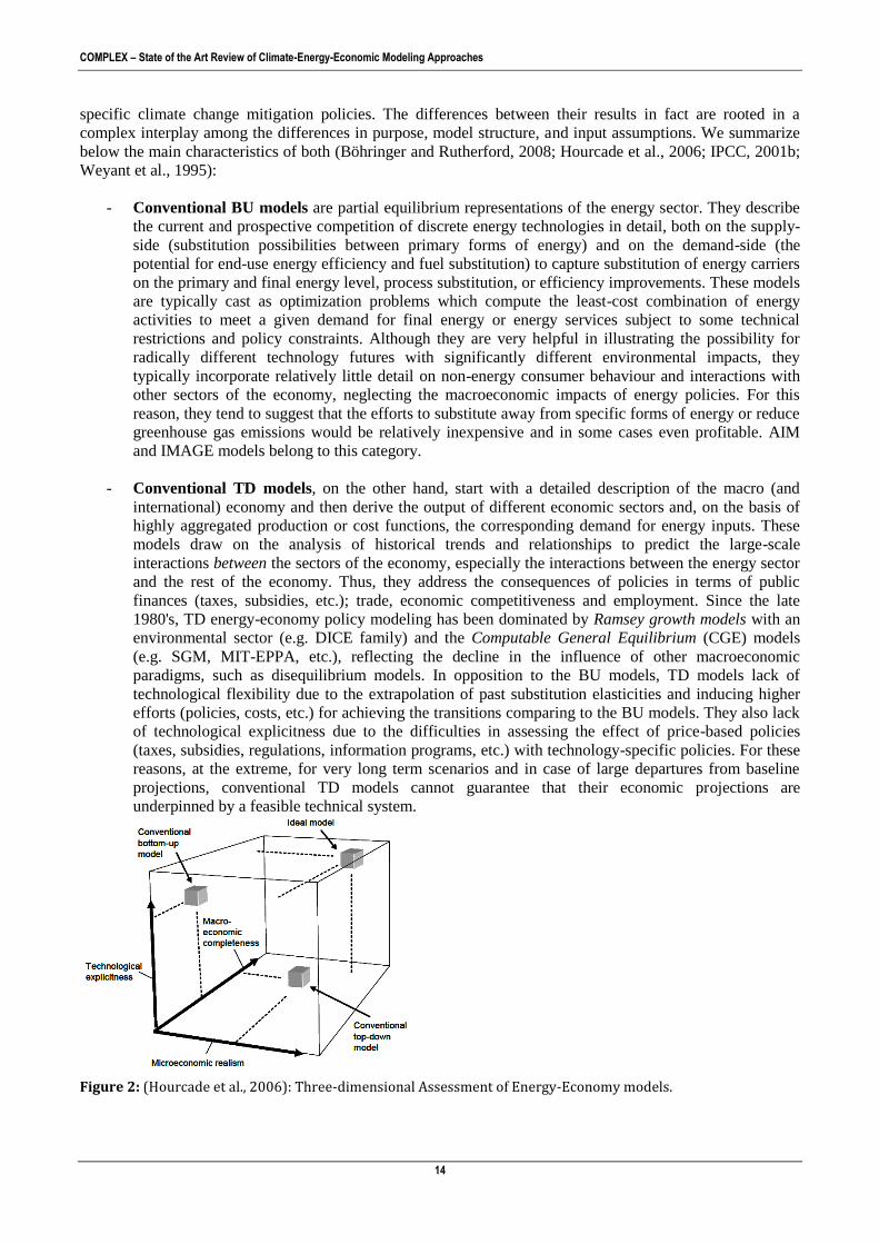
14
specific climate change mitigation policies. The differences between their results in fact are rooted in a
complex interplay among the differences in purpose, model structure, and input assumptions. We summarize
below the main characteristics of both (Böhringer and Rutherford, 2008; Hourcade et al., 2006; IPCC, 2001b;
Weyant et al., 1995):
- Conventional BU models are partial equilibrium representations of the energy sector. They describe
the current and prospective competition of discrete energy technologies in detail, both on the supply-
side (substitution possibilities between primary forms of energy) and on the demand-side (the
potential for end-use energy efficiency and fuel substitution) to capture substitution of energy carriers
on the primary and final energy level, process substitution, or efficiency improvements. These models
are typically cast as optimization problems which compute the least-cost combination of energy
activities to meet a given demand for final energy or energy services subject to some technical
restrictions and policy constraints. Although they are very helpful in illustrating the possibility for
radically different technology futures with significantly different environmental impacts, they
typically incorporate relatively little detail on non-energy consumer behaviour and interactions with
other sectors of the economy, neglecting the macroeconomic impacts of energy policies. For this
reason, they tend to suggest that the efforts to substitute away from specific forms of energy or reduce
greenhouse gas emissions would be relatively inexpensive and in some cases even profitable. AIM
and IMAGE models belong to this category.
- Conventional TD models, on the other hand, start with a detailed description of the macro (and
international) economy and then derive the output of different economic sectors and, on the basis of
highly aggregated production or cost functions, the corresponding demand for energy inputs. These
models draw on the analysis of historical trends and relationships to predict the large-scale
interactions between the sectors of the economy, especially the interactions between the energy sector
and the rest of the economy. Thus, they address the consequences of policies in terms of public
finances (taxes, subsidies, etc.); trade, economic competitiveness and employment. Since the late
1980's, TD energy-economy policy modeling has been dominated by Ramsey growth models with an
environmental sector (e.g. DICE family) and the Computable General Equilibrium (CGE) models
(e.g. SGM, MIT-EPPA, etc.), reflecting the decline in the influence of other macroeconomic
paradigms, such as disequilibrium models. In opposition to the BU models, TD models lack of
technological flexibility due to the extrapolation of past substitution elasticities and inducing higher
efforts (policies, costs, etc.) for achieving the transitions comparing to the BU models. They also lack
of technological explicitness due to the difficulties in assessing the effect of price-based policies
(taxes, subsidies, regulations, information programs, etc.) with technology-specific policies. For these
reasons, at the extreme, for very long term scenarios and in case of large departures from baseline
projections, conventional TD models cannot guarantee that their economic projections are
underpinned by a feasible technical system.
Figure 2: (Hourcade et al., 2006): Three-dimensional Assessment of Energy-Economy models.

COMPLEX – State of the Art Review of Climate-Energy-Economic Modeling Approaches
15
A number of modeling teams are developing hybrid models seeking to incorporate the advantages and
compensate for the limitations of both approaches. Different methodologies exist, such as linking
independently developed bottom-up and top-down (e.g. BU MARKAL and TD MIT-EPPA or BU
MESSAGE and TD MACRO) or directly building original hybrid models (e.g. IMACLIM models17
, WITCH
(Bosetti et al., 2006), E3MG (Barker et al., 2006)) (Böhringer and Rutherford, 2008; Hourcade et al., 2006).
Finally, another methodology is to modify former conventional BU or TD models in order to “hybridize”
them i) coupling a BU macroeconomic model with an energy model (e.g. MIT-EPPA, MERGE), ii) coupling
an energy model with a partial representation of the economy (e.g. MiniCAM/GCAM, POLES).
6) Energy sources considered As stated before, conventional TD models tend to describe the energy system as highly aggregated, while
conventional BU models tend to describe the current and prospective competition of discrete energy
technologies in detail, both on the supply and on the demand-side. Thus, in the latter, energy sources are often
highly disaggregated considering individually all current and potential important sources of energy: fossil
fuels (oil, gas and coal, including conventional and non-conventional), uranium, and renewable (hydro, solar,
wind, geothermal, oceanic, etc.).
Greenhouse gas emissions scenarios most commonly used in climate projections are derived from the Special
Report on Emissions Scenarios (IPCC SRES, 2000), published by the Intergovernmental Panel on Climate
Change. The original 40 scenarios reported in SRES have recently been rationalized into 4 Representative
Concentration Pathways (RCPs) (Moss et al., 2010; Vuuren et al., 2011a) which are fundamentally driven by
similar socio-economic models and cover a similarly wide range of future fossil fuel consumption scenarios as
those in the SRES (IPCC SRES, 2000). Energy resources estimations in most climatic IA models are based on
(IPCC SRES, 2000), which main sources were (Gregory and Rogner, 1998; Rogner, 1997) assessments.
However, recent historical data and analysis suggest that this estimations might be out of date (for a review
see for example (Höök and Tang, 2013; Ward et al., 2012)).
Uranium resources are usually estimated not to limit the expansion of nuclear power (e.g. GCAM (Calvin et
al., 2009)), although in some models such as MERGE and REMIND nuclear expansion can be constrained by
the depletion of uranium after the middle of this century (Edenhofer et al., 2010).
Renewable energies are also assumed to have large potentials. As reviewed in the “Special Report on
Renewable Energy Sources and Climate Change Mitigation” (IPCC, 2011): “all scenarios assessed confirm
that technical potentials will not be the limiting factors for the expansion of RE [renewable energies] at a
global scale”.
In general, models try to predict which technologies will dominate in a carbon-constrained future (and which
ones will stay negligible), and the reasons and speed for it. In power sector, capital and M&O costs (through
learning curves estimations), fuel use, lifetime, capacity factors, etc. are considered for each technology, as
well as specific characteristics such as penalties to renewable due to their intermittent generation.
Due to the long-term scope of the analysis (100 years and more) IA models consider technologies that are
currently in R&D stages and that might be developed over some decades or, on the contrary they also might
never deploy at significant level. Costs, efficiencies and appearance date of them are thus highly speculative.
Examples are Carbon Storage and Sequestration (CCS), further bioenergy technologies (e.g. cellulosic crops,
algae), nuclear IV generation (e.g. fast breeder), hydrogen, etc. These technology options can even be
combined as for example bioenergy and CCS (also known as BECCS) enabling the removal of CO2 from the
atmosphere (e.g. (Edmonds et al., 2013)). In order to dealing with uncertainties related with these technology
developments, different methodologies are applied. One approach is to combine their effects aggregating them
as generic technology improvements. Another approach is to analyse the sensitivity of each model to different
technology availability scenarios (e.g. (Edenhofer et al., 2010; Edmonds et al., 2013)).
7) Mitigation strategies/policies considered
17 Description of IMACLIM models < http://www.imaclim.centre-cired.fr/spip.php?rubrique1&lang=en >

COMPLEX – State of the Art Review of Climate-Energy-Economic Modeling Approaches
16
Policy-makers widely agree at the international annual Climate Change Conferences on the need of stabilizing
climate “at a level that would prevent dangerous anthropogenic interference with the climate system”
(UNFCCC, 1992). According to (IPCC, 2007b), “an upper limit beyond which the risks of grave damage to
ecosystems, and of nonlinear responses, are expected to increase rapidly” would be a 2ºC global mean
temperature increase above pre-industrial levels at equilibrium, i.e. 450 ppm CO2-equivalent.18
This level has
recently been related with a radiative forcing of 2.6 W/m2 in the new RCP process (Vuuren et al., 2011a).
All mitigation strategies in IA models require setting a price on carbon (explicitly through a carbon tax or
implicitly through a carbon cap applying inverse methods). Without it, the required structural shifts and
technological developments of current R&D technologies would never happen at a significant level.
Moreover, climate stabilization feasibility depends critically on the early and full participation of all countries
(e.g. (Clarke et al., 2009; Luderer et al., 2009)).
In the IPCC 4th Assessment Report (IPCC, 2007b), only three models containing 6 out of a total of the 177
mitigation scenarios presented results for the lowest category of a radiative forcing (2.5 – 3.0 W/m²). Since
costs generally increase non-linearly (exponentially) with the stringency of the concentration target, low
concentration targets are challenging. However, exploring low stabilization targets has become increasingly
relevant in the last years due to the increasing awareness of potential large impacts(Barnosky et al., 2012;
Edenhofer et al., 2010; Hansen et al., 2007; Lenton et al., 2008; Smith et al., 2009; Stern, 2006). This has
stimulated the interest in the most challenging scenarios and how to achieve them in the short-term.
The “EMF 22 International Scenarios” (Clarke et al., 2009) focused into low targets feasibility comparing the
results of 14 model: roughly half of them achieved 450 CO2-equivalent targets with full and immediate
participation due to the large and rapid changes required in energy and related systems to meet this ambitious
target (only 2 models, ETSAP-TIAM and MiniCAM-Base solved for the delayed scenario).
Figure 3: (Clarke et al., 2009): The scenarios submitted by the participating modeling teams. The “+” means that the team was able to produce the scenario; darkened cells with an “X” mean that the team was not able to produce the scenario. “N/A” means that the scenario was not attempted with the given model or model version.
18 However, others studies have reached conclusions that point that global warming of more than 1°C relative to
2000, will constitute “dangerous” climate change as judged from likely effects on sea level and extermination of
species’ (Hansen et al., 2006). (Hansen et al., 2008) concluded that CO2 concentrations should not trespass 350 ppm
in order to avoid slow climate feedbacks. Probabilistic assessments have also been made that demonstrate how
scientific uncertainties and different normative judgments on acceptable risks determine these assessments
(Mastrandrea and Schneider, 2004).

COMPLEX – State of the Art Review of Climate-Energy-Economic Modeling Approaches
17
More recently, numerous studies using a wide range of models such as AIM, IMAGE, MESSAGE, GCAM,
GET, MERGE, REMIND, POLES, TIMER (Azar et al., 2010; Calvin et al., 2009; Edenhofer et al., 2010;
Luderer et al., 2012; Masui et al., 2011; Rao et al., 2008; Riahi et al., 2011; Thomson et al., 2011; Vuuren et
al., 2011b, 2007) have shown that it is technically possible and economically viable to limit radiative forcing
(RF) to 2.6 W/m², if the full suite of technologies is available, all regions participate in emission reduction and
effective policy instruments are applied. A comprehensive review of these studies, however, shows that a
“magic bullet” does not exist: the mitigation strategies consist of a portfolio of measures. Although, different
models project many different pathways for evolving to a low-carbon energy system, all follow overshoot
mitigation trajectories, i.e. scenarios where the concentration is allowed to temporally increase over the final
target attained at the end of the simulation period.19
Also, land-use is found to be an important player and
modern bioenergy could contribute substantially to the mitigation targets. For an illustrative example of the
different mitigation strategies and carbon reduction paths. Therefore, these studies regularly conclude that
creating the right socio-economic and institutional conditions for stabilization (i.e. conditions for full and
immediate participation) will represent the most important step in any strategy towards GHG concentration
stabilization.
a)
b) Figure 4 : (a) (IPCC, 2007b) Cumulative emissions reductions for alternative mitigation measures for 2000-2030 (left-hand panel) and for 2000-2100 (right-hand panel). The figure shows illustrative scenarios from four models (AIM, IMAGE, IPAC and MESSAGE) aiming at the stabilization at low (490 to 540ppm CO2-eq) and intermediate levels (650ppm CO2-eq) respectively. Dark bars denote reductions for a target of 650ppm CO2-eq and light bars
19 This overshoot trajectory might be a problem in models considering non-linearities and climate thresholds.

COMPLEX – State of the Art Review of Climate-Energy-Economic Modeling Approaches
18
denote the additional reductions to achieve 490 to 540ppm CO2-eq. Note that some models do not consider mitigation through forest sink enhancement (AIM and IPAC) or CCS (AIM) and that the share of low-carbon energy options in total energy supply is also determined by inclusion of these options in the baseline. CCS includes CO2 capture and storage from biomass. Forest sinks include reducing emissions from deforestation. The figure shows emissions reductions from baseline scenarios with cumulative emissions between 6000 to 7000 GtCO2-eq (2000-2100). {WGIII Figure SPM.9}; (b) (Clarke et al., 2009) Global CO2 emissions and CO2-e concentrations in the overshoot 450 CO2-e scenarios with full participation. Model comparison analysis can help identify a range of pathways to a low carbon economy and shed light on the robustness of the associated cost estimates and technology options; for an overview of this literature see (Edenhofer et al., 2010, 2006). Thus, model results comparison enlighten some critical features (Clarke et al., 2009; Edenhofer et al., 2010):
- Without the availability of Carbon Capture and Storage (CCS) or the considerable extension of
renewables, the most ambitious mitigation pathway is not feasible.
- Bioenergy with CCS (BEECS) plays a crucial role due to its capacity to concur for negative emissions
(compulsory in overshoot scenarios): generally, models that consider it allow for low stabilization
scenarios while the ones that do not, are not able to reach the target (e.g. FUND (Tol, 2009)). In order
for BEECS to be a significant mitigation technology, bioenergy must deploy at large scale (150–
350EJ/yr primary energy toward the end of the century). Also, the assumed biomass potential
determines to a large extent the mitigation costs.
- Without any CCS, low stabilization is not possible and with a level of CCS that is low but sufficient
(120 GtC) to meet the low stabilization target, costs are still very high.
- (Edenhofer et al., 2010) found that nuclear power does not play an important additional role in
mitigation scenarios in most of the models compared. However, other models consider that this
energy source could become crucial in some scenarios (e.g. GCAM (Calvin et al., 2009)).
Despite the different mitigation portfolios in the models, model comparisons have commonly estimated
relatively modest mitigation costs in a range of 1.5 - 5.5% decrease of global GDP for 2050 (Edenhofer et al.,
2010; IPCC, 2007b) and 4 – 4.5 % to 2100 (Riahi et al., 2007).20
Unlike the other models, E3MG (Barker et
al., 2006) reports clearly different results concerning the mitigation costs, showing gains due to mitigation of
up to 2.1% for stabilization pathways (Edenhofer et al., 2010).
Although the sign of mitigation costs or benefices is not clear, in fact, a 5.5% reduction of world GDP to 2050
means less than 0.12% decrease in annual GDP. Losses of 4.5% to 2100 GDP translate into a loss of just
about two years of economic output or, in other words, the stabilization scenarios would achieve similar levels
of GDP as their corresponding baselines by 2102 instead of 2100. As argued by (Rosen and Guenther, 2013)
“Yet given all the uncertainties and variability in the economic results of the IAMs, […], the claimed high
degree of accuracy in GDP loss projections seems highly implausible. After all, economists cannot usually
forecast the GDP of a single country for one year into the future with such a high accuracy, never mind for the
entire world for 10 years, or more.”21
Summarizing, the projected macroeconomic costs of climate mitigation reported by the different IA models
are relatively modest, particularly compared to the scenario's underlying economic growth assumptions.
8) Temporal and spatial scales
Most of climate IA models have long and very long temporal scales because climate change is by nature a
long-term issue due to the huge inertia of global climate (Hansen et al., 2008). The time scale for climate
20 Other studies have reported higher costs in the order of 11% of 2100 GDP with PAGE model (Ackerman et al., 2009b). 21 Some simulation models recognize this shortcoming focusing into uncertainty and risk analysis (e.g. PAGE, ICAM, FUND).

COMPLEX – State of the Art Review of Climate-Energy-Economic Modeling Approaches
19
policy analysis is usually 100 years (IPCC, 2007a, 1990), although models can even go further in order to
reach climate stabilization conditions (e.g. MERGE and PAGE-09 (2200), MIND (2300) or FUND (3000)).
The temporal scale of a model defines the viewpoint of the represented system determining the relationships
between the variables considered. When doing short-term projections, variables as technology, population
evolution and capital stocks are roughly constant, although at medium and longer term demographic
transitions and innovations could induce changes in the economic structure and technological choices.
The study of the gas concentrations in the atmosphere usually requires a global spatial scope in IAM models,
although some national or regional levels are also used to analyse the efficacy and economic impacts of local
mitigation policies (for example, although AIM is a world model, it focus in the Asia-Pacific region). In
relation to the aggregation level, a high diversity exists from global-aggregated to regional-rich models,
although the majority of IA models consist on between 5 and 20 regions:
- Global-aggregated models (1 world region): e.g. DICE, ENTICE-BR, MIND, ANEMI.
- Medium-disaggregation (5-20 regions): e.g. MERGE, MESSAGE-MACRO, WITCH, GCAM,
ICAM, PAGE-09, FUND, MIT-EPPA, REMIND.
- High-disaggregation (>20 regions): e.g. POLES, WIAGEM, IM22
.
In fact, modeling trade-offs always exist between simplicity (aggregation) and complexity (disaggregation).
Thus, although highly regional disaggregated models would be in theory able to face more specific issues at
regional level, they also face an increasing number of assumptions and uncertainties. On the other hand,
global-aggregated models might face inconsistencies when considering that the world system evolves as a
homogenous unique entity. Also, models with high regional disaggregation are constrained to have lower
projection horizon (e.g. POLES and WIAGEM to 2050). The correct approach is to select the model which
assumptions are the most acceptable depending on the problem to study.
2.2.2 Specific review: the discount rate and quality concerns
Controversies involving the discount rate have been central to global welfare optimization climate models and
policy for many years (e.g. (Nordhaus, 2008)); a detailed overview of these issues can be found in Chapter 9
of the Stern Review (Stern, 2006).
Welfare23
optimization models maximize the discounted present value of welfare (which grows with
consumption, although at an ever diminishing rate) across all time periods simultaneously (as if decisions
could be made with perfect foresight) by choosing how many emissions to abate in each time period, where
abatement costs reduce economic output. Discounting is a method used in economic models to aggregate costs
and benefits over a long time horizon by summing net costs (or benefits), which have been subjected to a
discount rate typically greater than zero, across future time periods. This process also requires imputing
speculative values to non-market ‘goods’ like ecosystems or human lives. If the discount rate equals zero, then
each time period is valued equally (case of infinite patience). If the discount rate is infinite, then only the
current period is valued (case of extreme myopia). The discount rate chosen in IA models is critical, since
abatement costs will typically be incurred in the relatively near term, but the brunt of climate damages will be
realized primarily in the long term. Thus, if the future is sufficiently discounted, present abatement costs, by
construction, will outweigh discounted future climate damages, as discounting will eventually reduce future
damage costs to negligible present values (e.g. (Nordhaus, 2008; Schneider and Lane, 2005; Stanton et al.,
2009)). Considering a climate impact that would cost 1 billion dollars 200 years from now, a discount rate of
5% per year (a conventional value, e.g. DICE-07 (Nordhaus, 2008)) would make the present value of that
future cost equal to $58,000. And at a discount rate of 10% per year, the present value would only be $5.
22 Models are continuously in evolution. For example, IMAGE 1.0 model that was developed in the 80s, was a global (single-region) model to capture major cause–effect relationships making up the complex greenhouse problem (Bouwman et al., 2006). 23 “Welfare”, or ‘utility’, which is treated as a synonym for welfare in most models.
COMPLEX – State of the Art Review of Climate-Energy-Economic Modeling Approaches
20
Thus, in cost-benefit analysis models, mitigation decisions in the near-term to reduce future damages are
critically dependent on the discount rate. In models where non-linearities are considered, the discount rate is
even the parameter that most influences the 22nd century behaviour of the modelled climate (Schneider and
Lane, 2005).24
Thus, together with the common assumption that the world will grow richer over time, discounting gives
greater weight to earlier, poorer generations relative to later, wealthier generations. In their review, (Stanton et
al., 2009) conclude that equity between regions of the world at any time (thus at inter and intra-generational
level) is excluded from most IA models, even from those which explicitly treat the regional distribution of
impacts (that are projected to be worse in developing countries). In fact, in regionally disaggregated models,
any simple, unconstrained attempt to maximize human welfare would generate solutions that include large
transfers from rich to poor regions. To prevent this “problem” from dominating their results, IA models
employ “Negishi welfare weights” (based on theoretical analysis in (Negishi, 1972), which constrain possible
solutions to those which are consistent with the existing distribution of income. In effect, the Negishi
procedure imposes an assumption that human welfare is more valuable in richer parts of the world (Stanton et
al., 2009).
Few exceptions exist to these trends. For example, the FREE model (Fiddaman, 2002) uses a discount rate set
to 0 (so that the welfare of all generations is weighted equally) and the inequality aversion rate to 2.5 (instead
of lower common values of “1”), so that the needs of current (poorer) generations are of greater urgency. The
Stern Review (Stern, 2006) uses almost zero, hyperbolic discounting (0.001 yr-1
) and explore diverse
assumptions about the equity weighting attached to the valuation of impacts in poor countries.
Summarizing, current welfare optimization IA models typically discount future impacts from climate change
at relatively high rates. This practice may be appropriate for short-term financial decisions but its extension to
intergenerational environmental issues rests on several empirically and philosophically controversial
hypotheses.
2.3 Classification of climate IA models
Different classifications for IA models have been proposed in the literature depending on the focused
characteristics in the categorization. Also, after more than 20 years of development, there is a trend of model
hybridization that make that most classifications of IA models found in the literature allow for some overlap
between sub-groups of IA models (Arigoni and Markandya, 2009; Hourcade et al., 2006; Stanton et al., 2009).
In Section 2.2 we already presented an overview of the climatic IA models following the traditional BU vs.
TD classification of Energy-Economy models (Böhringer and Rutherford, 2008; Hourcade et al., 2006; IPCC,
2001b; Weyant et al., 1995). The economics module of IA models can also be used to distinguish between
Computable General Equilibrium models (CGE), Optimization models or Simulation models (Dowlatabadi,
1998).
The III Working Group of the IPCC (Weyant et al., 1995) used a two-dimensional classification for climate
IA models between policy-optimization and policy-evaluation models which has been extensively followed
thereafter in the literature (e.g. (Kelly and Kolstad, 1998; Tol, 2006; Toth, 2005)).25
24 For example, in the E-DICE model, a modified version of Nordhaus’ DICE which contains an enhanced damage function that reflects the likely higher damages that would result when abrupt climate changes occur, (Mastrandrea and Schneider, 2001) find that, for low discount rates, the present value of future damages creates a carbon tax large enough to keep emissions below the trigger level for the abrupt non-linear collapse of the THC a century later. A higher discount rate sufficiently reduces the present value of even catastrophic long-term damages so that abrupt non-linear THC collapse becomes an emergent property of the coupled socio-natural system. 25
In fact this classification is generic to computer models and thus prior to climate IA models (Sterman, 1991).

COMPLEX – State of the Art Review of Climate-Energy-Economic Modeling Approaches
21
- Policy-evaluation models take a small set of policies and policy proposals, and the consequences of
these policies are evaluated in a “what-if” exercise. Consequences are assessed with a more or less
formalized set of indicators of environmental quality and economic welfare, representing usually
impacts in great detail. There are many different simulation techniques, including stochastic
modeling, system dynamics, discrete simulation, and role-playing games. Classical representatives of
this family are AIM and IMAGE. Policy-evaluation models tend to be developed by natural scientists;
the models tend to be large, with considerable spatial and temporal details, and use to picture the
world as a strongly non-linear system with potential catastrophes. In fact, they can easily incorporate
feedback effects, non-linearities and dynamics since they are not rigidly determined in their structure
by mathematical limitations as optimization models often are.
- Policy-optimization models include a strictly formal, uni-dimensional assessment of “better” and
“worse” outcomes, and use this to select the “optimal” policy. Analytically, they optimise key policy
control variables such as carbon emission control rates or carbon taxes, given formulated policy goals
(e.g. maximising welfare or minimising the costs of meeting a carbon emissions or concentration
target). However, impacts are generally estimated in a more aggregated way. Different approaches are
used, such as cost-benefit analysis and cost-efficiency analysis. Examples of this category are: the
DICE family (RICE, SLICE, etc.), MiniCAM/GCAM, MERGE, MIT-EPPA, GTAP, etc. For a more
detailed discussion about these models see (Tol, 2006; Toth, 2005). Policy-optimization models tend
to be developed by economists, who often tend to normative solutions to policy problems
(optimization models are prescriptive, but simulation models are descriptive). These models are
usually small, with little spatial or temporal resolution, and depict the world as smooth and robust.
Different issues need different approaches to be faced. Optimization techniques should be always considered
whenever the meaning of best is well defined, and if the system to be optimized is relatively static and free of
feedback. Unfortunately, these conditions are rarely true for the social, economic, and ecological systems.
Thus, limitations of these models are: (i) difficulties with the specification of the objective function, (ii)
unrealistic linearity, (iii) lack of feedback and (iv) lack of dynamics (Sterman, 1991). Indeed, one of the main
uses of simulation models is to identify how feedback, nonlinearity, and delays interact to produce troubling
dynamics that persistently resist solution. (For examples see (Forrester, 1969; Sterman, 1985)). These models
do not calculate what should be done to reach a particular goal, but clarifies what would happen in a given
situation. The purpose of simulations may be foresight or policy design. Simulation models do have their
weak points, however. Most problems occur in the description of the decision rules, the quantification of soft
variables, and the choice of the model boundary (Sterman, 1991).
Tabel 1 classifies some of the most used IA models following the categories described before: BU vs. TD and
policy-optimization vs. policy-evaluation. In order to represent the hybrid characteristics of many models we
have avoided the representation in boxes, sorting them qualitatively along the axe BU vs. TD.
Finally, we briefly mention the classification proposed by (Stanton et al., 2009) who reviewed 30 significant
climate-economics models classifying them into 5 categories with some overlap: welfare maximization (e.g.
DICE family, AIM, MERGE, MIND, FUND), general equilibrium (e.g. MIT-EPPA, AIM, SGM, IMACLIM,
WIAGEM), partial equilibrium (e.g. MiniCAM), simulation (e.g. PAGE) and cost minimization (e.g. MIND,
MESSAGE). For a classification in relation to the level of integration, (Schneider and Lane, 2005) distinguish
between different “IAM generations”.

COMPLEX – State of the Art Review of Climate-Energy-Economic Modeling Approaches
22
Top-Down
(Macroeconomic model coupled
with an energy model)
Hybrid
(Energy model coupled with a
partial depiction of the economy)
Bottom-Up
Policy-
evaluation
AIM/Dynamic global
(Masui et al., 2006)
GTEM (Pant, 2007)
ANEMI (Akhtar et al.,
2013)
FREE (Fiddaman, 2002)
AIM/Emission- Linkage
(Morita et al., 2003)
E3MG (Barker et al., 2006)
AIM/Enduse (Kainuma,
2003)
IMAGE (Bouwman et
al., 2006)
PAGEc (Hope, 2011)
ICAMc (Dowlatabadi,
1998)
Policy-
optimization
DICE familya
GEM-E3 (Capros et al.,
2010)
GTAP-E (Burniaux and
Truong, 2002)
SGM (Edmonds et al.,
2004)
Phoenix (Fisher-Vanden
et al., 2012)
WIAGEM (Kemfert,
2005)
MERGE (Manne and Richels,
2004)
MIT-EPPA 4 (Paltsev et al.,
2005)
REMIND-R (Leimbach et
al., 2010)
IMACLIM-R (Sassi et al.,
2010)
MIND (Edenhofer et al.,
2005)
MARKAL-MACRO
(Loulou et al., 2004)
MESSAGE-MACRO (Rao
et al., 2006)
WITCH (Bosetti et al.,
2006)
GCAM/MiniCAM (Clarke et al.,
2007)
POLES (JCR EC, 2010)
MARKAL (Seebregts et
al., 2002)
MESSAGE (Messner and
Strubegger, 1995)
FUNDb (Anthoff and Tol, 2012)
Tabel 1: Representative Climatic IAM model classification following the axes policy-optimization vs. policy evaluation and bottom-up vs. top-down. aDICE family includes: DICE (Nordhaus, 2008), RICE (Nordhaus, 2010), ENTICE (Popp, 2006), AD-RICE among others; bFUND can run different optimization modes, among them: top-down vs. bottom-up; c Stochastical evaluation models PAGE and ICAM does not focus into energy neither economy, but on risk and uncertainties. Thus, it cannot be classified following the conventional axes for Energy-Economy models BU vs. TD.

COMPLEX – State of the Art Review of Climate-Energy-Economic Modeling Approaches
23
2.4 Discussion on the state of the art of IAM
After 25 years of development, climatic IAM now represents a fundamental tool when assessing mitigation
strategies, estimating the costs and informing decision makers in order to prevent anthropogenic climate
change. It is even beginning to be used to evaluate the mitigation-adaptation trade-offs. Significant
improvements have been done since early 90s, when IAM was inexpert and subject to severe and pertinent
critics (e.g. (Risbey et al., 1996; Weyant et al., 1995)). In the words of (Tol, 2006): “IAM is now an
accepted way of doing research and advising policy, in climate change, in acidification, and increasingly in
other areas. IA models have developed from crude and clumsy tools to sophisticated frameworks that can
answer many of the questions that stakeholders may have.”
The overview of the development of IAM shows that the field has evolved in close relation with the IPCC
process and Assessments due to the adoption of the “consensus approach” as the strategy to deal with
scientific uncertainties in the interface between science and policy (e.g. (van der Sluijs et al., 2010)).
However, IA models still face different challenges. IA models are limited by the weaknesses in their
underlying knowledge and by the simplifications required for efficient modeling and simulation. Critics
point out that many models suffer from a lack of transparency in terms of both policy relevance and
credibility, since building these models inevitably involves numerous judgment calls, debatable arguments
and untestable hypothesis that turn out to be of great importance in determining the policy
recommendations of these models. Some controversial characteristics include: the dominant sequential
approach, the difficulty to represent pervasive technological developments and non-linearities, thresholds
and irreversibilities, the treatment of climate change damages, the omission of other human-disturbances,
the discount rate values, the consideration of equity across time and space, structural shifts in socio-
economic systems, etc.
Although since 90s climate IA models have improved their policy-relevance26
(the assessment part), the
coupling of natural and social science models (the integration part) has largely stalled. The sequential
approach has been used extensively in spite of really integrated structures as the full-integrated scheme
showed in the Figure 4 (a). Also, climate IA models generally omit other human-disturbances such as the
biodiversity loss, the alteration of other natural cycles (e.g. nitrogen, phosphorus, water), etc. that are in
reality tightly coupled between them and with the climate system (e.g. (MEA, 2005; Rockström et al.,
2009)).
Models that traditionally include rich couplings among the natural subsystems are known as Earth System
Models (ESM). Although their focus was originally on the physical climate system, more recently the
carbon cycle and dynamic vegetation have been added. On the other hand, the IAM approach comes largely
from a tradition of modeling the interaction of human activities, decision making and the environment,
focusing on economic production and consumption, energy systems, emissions and climate change.27
Thus,
although there is a significant overlap in the systems modelled, there are also components that are unique to
each group (Hibbard et al., 2010; Tol, 2006; Vuuren et al., 2011c). As (Tol, 2006; Vuuren et al., 2012,
2011c) argue, one of the main challenges to future IAM developments is the full-coupling with the Earth
System Models (ESM): “[…] if ESM want to truly describe and predict the earth system, they would need
to include the major agent of global change, namely homo sapiens sapiens” (Tol, 2006) pointing out the
difficulties of mapping from natural to economic space and back (down-scaling and up-scaling in a
mismatch of scales28
), and relating mental models of the economic agents (generally operating in the short-
term) with the natural agents “reactions” (characterized by big inertias of decades and centuries).
26 Indeed, the IPCC has reached a great level of reputation, trust, and network for both the scientists and policy-makers, which culminated with the award of the 2007 Peace Nobel Price. 27 (Tol, 2006) indicates that integrated assessment models “may be classified as simple earth system models”. 28 For example, how to downscale climate change from grids that are usually in the order of hundreds of kilometers when studying the impacts in biodiversity in the mosaic of “small” ecosystems of the planet? How can a climate modeler scale up knowledge of evapotranspiration through the sub-millimeter-sized stomata of forest leaves into the hydrological cycle of the climate model, resolved in this hundreds of kilometers grids?

COMPLEX – State of the Art Review of Climate-Energy-Economic Modeling Approaches
24
Because this interplay between natural and socio-economic systems determines the entire system’s
evolution, the representation of the corresponding feedbacks is critical to the development of appropriate
climate change adaptation and mitigation strategies, the potential to represent non-linearities, thresholds,
irreversibilities and positive feedbacks. That is why the latest developments focus on these issues:
- Heightened collaboration between impacts, adaptation and vulnerability research, and climate and
integrated assessment modeling (Calvin et al., 2013; Hibbard et al., 2010; Moss et al., 2010).
- Coupling of IAMs with models that include rich couplings among the natural subsystems as Earth
System Models (ESM) (Tol, 2006; Vuuren et al., 2011c), e.g. GCAM with CESM (Jones et al.,
2011), MIT-EPPA as a module of MIT-IGSM (Sokolov et al., 2005), GISMO project (PBL, 2008).
Feedbacks between the subsystems remain as a scarce, partial and constrained by critical uncertainties
characteristic of the current development of IA models, as revealed by the survey of damage functions
(Arigoni and Markandya, 2009). Although some evolution exists, recent surveys conclude that it has been
significantly slow in the last decade.
The choice of the discount rate in welfare optimization models has a very large effect on policy
recommendations, because most impacts of climate change occur in the future while mitigation takes place
in the near term. Higher discount rates lead to lower present values of future damages. The choice of the
discount rate was one of the main controversies in the (Stern, 2006) Report. This is an issue inherent to the
economics of climate change and not just to IAM, though the longer time horizons in these models make
this issue more important. Another sensitive assumption is the way to weight impacts in different regions,
when aggregating global values
Uncertainty and risk aversion analysis (when considered by the model) is crucial in IAM, and related to
this, whether best guess / central values are used or not. A key issue here regards to climate sensitivity, i.e.
the equilibrium warming expected with a doubling of CO2 concentrations, and the risk of low probability-
high consequence events29
.
There have been rapid advances in recent years in the area of including endogenous technological change;
the review by (Kahouli-Brahmi, 2008) offers a thorough description of the most recent attempts to model
endogeneity and induced technological innovation.
A review of the recent literature on IAM shows that most models agree that low climate stabilization (below
2ºC) is technically and economically viable if the full suite of technologies is available, all regions
participate in emission reduction and effective policy instruments are applied. However, comparing the
results of the different models we find that there is not one single mitigation strategy. On the contrary, there
are different mitigation strategies consisting of a portfolio of measures, which may vary depending on the
specific model used. However, without the availability of CCS or the considerable extension of renewable
energies, the most ambitious mitigation pathways are not feasible. Thus, the conditions of global
participation in climate policy in the near-term and shift technology transfer across regions remain as the
greatest challenge for low stabilization targets.
The utility of the climate IAM based on Cost-Benefit Analysis has been greatly disputed since its start due
to the number of “empirically and philosophically controversial hypotheses”, as discussed in the text.
Several authors argue that climate change policy should be reframed as “buying insurance against
catastrophic, low-probability events”, i.e. assuming the critical uncertainties and plaid to adopt the
Precautionary Principle for policy decisions (e.g. (Ackerman et al., 2009a; Rosen and Guenther, 2013;
Weitzman, 2009)), arguing that “the appropriate role for economists would then be to determine the least-
cost global strategy to achieve the stabilization target” (Ackerman et al., 2009a). Finally, Climatic IAM
must be seen as a science in continuous evolution, in which new dimensions of the problem have to be
incorporated by using new methodologies and scopes, and models have to integrate continuously new
scientific knowledge and deepen and diversify the assessments.
29 This is especially relevant due to the limited ability of current climate IA models to represent potential non-linearities, thresholds and irreversibilities.
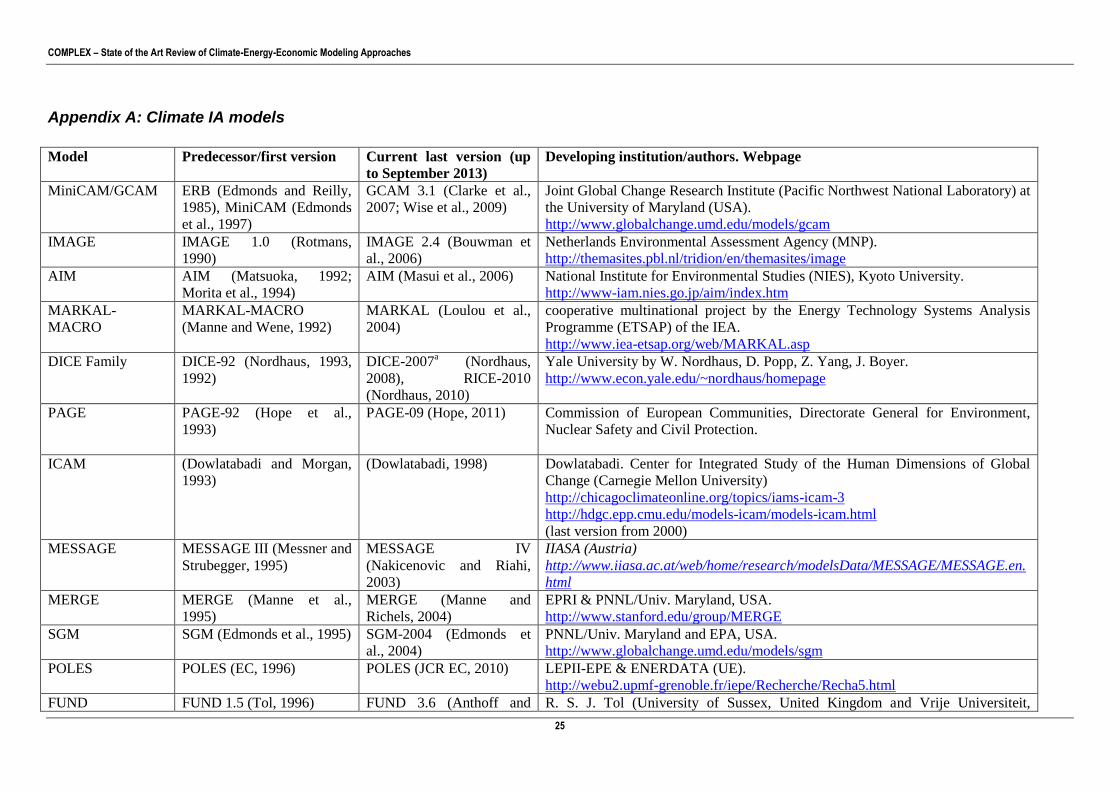
COMPLEX – State of the Art Review of Climate-Energy-Economic Modeling Approaches
25
Appendix A: Climate IA models
Model
Predecessor/first version Current last version (up
to September 2013)
Developing institution/authors. Webpage
MiniCAM/GCAM
ERB (Edmonds and Reilly,
1985), MiniCAM (Edmonds
et al., 1997)
GCAM 3.1 (Clarke et al.,
2007; Wise et al., 2009)
Joint Global Change Research Institute (Pacific Northwest National Laboratory) at
the University of Maryland (USA).
http://www.globalchange.umd.edu/models/gcam
IMAGE
IMAGE 1.0 (Rotmans,
1990)
IMAGE 2.4 (Bouwman et
al., 2006)
Netherlands Environmental Assessment Agency (MNP).
http://themasites.pbl.nl/tridion/en/themasites/image
AIM AIM (Matsuoka, 1992;
Morita et al., 1994)
AIM (Masui et al., 2006) National Institute for Environmental Studies (NIES), Kyoto University.
http://www-iam.nies.go.jp/aim/index.htm
MARKAL-
MACRO
MARKAL-MACRO
(Manne and Wene, 1992)
MARKAL (Loulou et al.,
2004)
cooperative multinational project by the Energy Technology Systems Analysis
Programme (ETSAP) of the IEA.
http://www.iea-etsap.org/web/MARKAL.asp
DICE Family DICE-92 (Nordhaus, 1993,
1992)
DICE-2007a (Nordhaus,
2008), RICE-2010
(Nordhaus, 2010)
Yale University by W. Nordhaus, D. Popp, Z. Yang, J. Boyer.
http://www.econ.yale.edu/~nordhaus/homepage
PAGE
PAGE-92 (Hope et al.,
1993)
PAGE-09 (Hope, 2011) Commission of European Communities, Directorate General for Environment,
Nuclear Safety and Civil Protection.
ICAM (Dowlatabadi and Morgan,
1993)
(Dowlatabadi, 1998) Dowlatabadi. Center for Integrated Study of the Human Dimensions of Global
Change (Carnegie Mellon University)
http://chicagoclimateonline.org/topics/iams-icam-3
http://hdgc.epp.cmu.edu/models-icam/models-icam.html
(last version from 2000)
MESSAGE MESSAGE III (Messner and
Strubegger, 1995)
MESSAGE IV
(Nakicenovic and Riahi,
2003)
IIASA (Austria)
http://www.iiasa.ac.at/web/home/research/modelsData/MESSAGE/MESSAGE.en.
html
MERGE MERGE (Manne et al.,
1995)
MERGE (Manne and
Richels, 2004)
EPRI & PNNL/Univ. Maryland, USA.
http://www.stanford.edu/group/MERGE
SGM SGM (Edmonds et al., 1995) SGM-2004 (Edmonds et
al., 2004)
PNNL/Univ. Maryland and EPA, USA.
http://www.globalchange.umd.edu/models/sgm
POLES POLES (EC, 1996) POLES (JCR EC, 2010) LEPII-EPE & ENERDATA (UE).
http://webu2.upmf-grenoble.fr/iepe/Recherche/Recha5.html
FUND FUND 1.5 (Tol, 1996) FUND 3.6 (Anthoff and R. S. J. Tol (University of Sussex, United Kingdom and Vrije Universiteit,

COMPLEX – State of the Art Review of Climate-Energy-Economic Modeling Approaches
26
Tol, 2012) Netherlands) and D. Anthoff (University of Michigan, USA).
http://www.fund-model.org
GTEM MEGABARE (Hinchy and
Hanslow, 1996)
GTEM (Pant, 2007) Australian Bureau of Agricultural and Resource Economics and Science
(ABARES).
http://www.daff.gov.au/abares/models
GEM-E3 GEM-E3 (Capros et al.,
1998)
GEM-E3 (Capros et al.,
2010)
http://ipts.jrc.ec.europa.eu/activities/energy-and-transport/gem-e3
WIAGEM WIAGEM (Kemfert, 2002) WIAGEM (Kemfert, 2005) Humboldt University and DIW Berlin, Germany.
GTAP-E GTAP-E (Burniaux and
Truong, 2002)
GTAP-E (McDougall and
Golub, 2007)
Global network administered by the Center for Global Trade Analysis in Purdue
University (USA).
https://www.gtap.agecon.purdue.edu/models/energy/default.asp
FREE FREE (Fiddaman, 2002) Thomas Fiddaman.
http://www.metasd.com/models/#Climate
MIND MIND (Edenhofer et al.,
2005)
MIND (Held et al., 2009) Esto parece que lo lleva edenhofer et al del PIK.
http://www.pik-potsdam.de/research/sustainable-solutions/models/
WITCH WITCH (Bosetti et al., 2006) Fondazione Eni Enrico Mattei (FEEM) Italy.
http://www.witchmodel.org/
E3MG E3MG (Barker et al., 2006) E3MG (Barker et al., 2006) UK Tyndall Centre for Climate Change Research
http://www.4cmr.group.cam.ac.uk/e3mg
REMIND REMIND (Leimbach et al.,
2010)
REMIND 1.5 (Luderer et
al., 2013)
PIK, Germany.
http://www.pik-potsdam.de/research/sustainable-solutions/models/remind/remind-
code
IMCALIM-R IMACLIM-R (Sassi et al., 2010) Centre International de Recherche sur l’Environnement et le Développement
(CIRED), France.
http://www.imaclim.centre-cired.fr
ANEMI ANEMI_1 (Davies and
Simonovic, 2010)
ANEMI_2 (Akhtar et al.,
2013)
University of Western Ontario, Canada.
MIT-EPPA MIT-EPPA 1.6 (Yang et al.,
1996)
MIT-EPPA 4.1 (Paltsev et
al., 2005)
MIT, USA.
http://globalchange.mit.edu/research/IGSM/eppadl
Phoenixb Phoenix (Fisher-Vanden et al., 2012) PNNL/Univ. Maryland and EPA, USA.
www.globalchange.umd.edu/models/phoenix/
Tabel 2: The majority of IAM projects are independent efforts; however, there is much collaboration within the IAM field. For example, model developers frequently meet at conferences and workshops to discuss their results and share information (e.g. EMF). aDICE-2013 is in beta-version (http://www.econ.yale.edu/~nordhaus/homepage/Web-DICE-2013-April.htm). bIn fact, the Phoenix model replaces the Second Generation Model (SGM) that was formerly used for general equilibrium analysis at JGCR

COMPLEX – State of the Art Review of Climate-Energy-Economic Modeling Approaches
27
3. Overview of Environmental Computational General Equilibrium Models
3.1 Introduction
CGE models are based on Walrasian general equilibrium theory. This theory prevails when supply and
demand are equalized across all of the interconnected markets in the economy. These models are
simulations that combine the general equilibrium structure with realistic economic data to solve numerically
for the levels of supply, demand and price that support equilibrium across a specified set of markets. CGE
have become increasingly popular over the last couple of decades and are now the dominating model type
for economic policy analysis. Main CGE applications are in fiscal reform and development planning,
environmental analysis and, international trade. However, as discussed above CGEs, like other traditional
models, suffer from some strong (even wrong) assumptions, which can lead to unwarranted conclusions for
policy making.
In the literature a clear definition of CGE models is missing, i.e. there is still much discussion about a
definition. In the literature also different names can be found for CGE models, such as Transaction Value
models, Applied General Equilibrium models and SAM-based general equilibrium, see e.g. Thissen (1998).
Borges (1986) defines CGE-models as models that “describe the allocation of resources in a market
economy as the result of the interaction of supply and demand, leading to equilibrium prices. The building
blocks of these models are equations representing the behavior of the relevant economic agents- consumers,
producers, the government, etc. Each of these agents’ demands or supplies goods, services and factors of
production, as a function of their prices.” This definition does not exclude models that are generally not
seen as CGE models.
Thissen (1998), following Bergman (1990), tries to solve this by narrowing the definition of CGE models
by describing their common and distinct characteristics, such as aggregation of households and the
modeling of all links within the economy that represent a transaction of money or goods, opposite to partial
equilibrium models that analyze the different sectors separately under ceteris paribus assumptions. The idea
of CGE models is to compare the base equilibrium with the new equilibrium that arises after t exogenous
shocks or the policy measures arise. Bergman and Henrekson (2003) also state that a precise definition of a
CGE model does not exist. Whenever the CGE model “label” is used “the model in question tends to have
certain specific features”, they state. One of these (very basic) features is that the model should be “a multi-
sector model based on real world data of one or several national economies.” For a thorough discussion on
the definition of CGE models we refer to the mentioned papers above.
A standard CGE model is characterized by flexible disaggregation and pre-programmed alternative rules for
clearing factor markets and macro accounts. Fig. 3 provides a simplified picture of building blocks of a
standard CGE and the links between the major them. The disaggregation of activities, (representative)
households, factors, and commodities – the blocks on the left side of the figure – is determined by the
disaggregation of the SAM. The arrows represent payment flows. With the exception of taxes, transfers and
savings, the model also includes “real” flows (for a factor service or a commodity) that go in the opposite
direction. The activities (which carry out production) allocate their income, earned from output sales, to
intermediate inputs and factors.
Since the beginning of the 1990´s CGE modeling has also become a widely used tool for analysis of
environmental policy and natural resource management issues. The main purpose of this chapter is to
review this branch of CGE modeling.

COMPLEX – State of the Art Review of Climate-Energy-Economic Modeling Approaches
28
Figure 5: (Strzepek et al 2008) Links between building blocks of a standard CGE
3.2 Classification of CGE models
In spite of these basic similarities or characteristics that are used to define CGE models, there are also
significant differences between individual CGE models, and a number of categories of CGE models can be
distinguished. In the literature there are several ways to classify CGE models. Thissen (1998) describes
three different ways to classify CGE models. The first classification is based on historical development,
where two types can be distinguished. The first type of this historical classification is evolved from macro
models (or multisector models) in the 1970s, commonly used for policy analysis in developing countries.
The second type of this historical classification, Walrasian CGE models, are develop from the general
equilibrium framework of Walras and the numerical solution of these systems by Scarf (1967). The second
classification by Thissen (1998) deals with the choice of so called “closure rules”, here the distinction is
between Walrasian CGE models, that are considered a subgroup of all CGE models with a neoclassical
closure and other CGE models that have other “closures” (e.g. Johansen closure, Keynes closure etc.). The
third classification of CGE models is based on the techniques used to determine the parameter values. Here
we have to different types, the first based on calibration techniques also knows and SAM-based and second
models with parameters based on econometric estimation.
An alternative classification is static and dynamic CGE models. Several static CGE models have been used
for multi-period analyses in which prices are set in each time period and then this solution is used as the
initial point for the next period. In a dynamic economic model, forward looking behavior on the part of
households and firms is assumed and stock accumulation relations are explicitly included, however, CGE’s
assuming no foresight at all. Therefore dynamic CGE models are better described as ‘quasi dynamic’ or
‘recursive dynamic’ models. This brings us also to the downside of these models as no transaction takes
place in dis-equilibrium that is all economic agents have to wait until equilibrium is found before they make
any decision.
In addition to the static-dynamic dimension it is useful to distinguish between single-country, multi-country
and global models. Single-country models tend to be more detailed in terms of sectors and household types,
and they are in general used for analyses of country-specific policy issues and proposals. Multi-country and
global models, on the other hand, tend to have less sector detail and to be designed for analysis of proposed
multi-lateral policies such as free-trade agreements. In the case of environmental CGE models the multi-
country and global models in most cases are designed for analysis of trans-boundary pollution problems.
Finally CGE can also differ in number of production sectors, number of primary factors and specification of
international trade relations.
The specification of international trade relations is an important aspect of all open-economy CGE models,
but seems particularly important in environmental CGE models. The most widely used approach is to adopt
the “Armington assumption”, which implies that goods with the same statistical classification but different
countries of origin are treated as non-perfect substitutes. This is done to overcome extreme patterns of

COMPLEX – State of the Art Review of Climate-Energy-Economic Modeling Approaches
29
specialization that occurs since in most CGE models there are more sectors than factors. Another way to
overcome overspecialization in CGE models is to retain the assumption about exogenously given terms of
trade, while relative-price dependent export supply functions are added. These functions usually are derived
from constant elasticity of transformation (CET) functions defining the output of a given sector as a
revenue-maximizing aggregate of goods for the domestic market and goods for foreign markets.
3.3 Environmental CGE review
Using a CGE model for policy analysis is conditional on whether the proposed policy measures are likely to
have general equilibrium effects. Some environmental problems may be quite costly for some firms and
households, the repercussions to the rest of the economy often are small or close to zero. However, there are
indeed major environmental problems with a much wider geographic and economic scope. A prime
example is “climate change”, which is related to emissions of carbon dioxide and other greenhouse gases.
Many CGE models are widely used for evaluation of climate related policies. The CGE models analyzed
may be all classified as energy–economy–environment models since they are all concerned with linkages
between economic activities, energy transformation, and associated environmental impacts. We find that
operational versions of E3–CGE models have a good coverage of central economic indicators.
Environmental indicators such as energy related emissions with simple direct links to economic activities
are widely covered, whereas indicators with complex natural science background such as water stress or
biodiversity loss are hardly represented. Social indicators stand out for very weak coverage, mainly because
they are vaguely defined or incommensurable.
Despite this heavy usage of CGE models in policy analysis, these models are often criticized as being
insufficiently validated. Key parameters are often not econometrically estimated, and the performance of
the model as a whole is rarely checked against historical outcomes. As a consequence, questions frequently
arise as to how much faith one can put in CGE results. In the literature there exist several ways to validate
CGE models. One way to validate a policy model is to test it against historical data, and examine how well
the model explains past events. By doing so, any deficiencies in the model can be better understood, and
work can be done to improve them. If CGE models are capable of capturing the impact of important policy
events, then confidence would be built in applying a model with the same theoretical structure to later
experiments. Special attention goes to (energy-related) elasticities, most CGE models derived the value of
these elasticities based on the literature, however some use econometric estimation.
Within the class of environmental CGE models two other classification can be found. The first one is
externality CGE Models, i.e. CGE models focused on climate change which deal with externalities and
policies aimed at internalizing externalities. And the second deals with resource management CGE Models,
i.e. climate change or environmental problems which reflect any kind of market failure leading to poor
management of natural resources and losses of environmental amenities. Thus in economies highly
dependent on natural resources like forests, fisheries, agricultural land or grazing land changes in the natural
resource management regime may have economy-wide effects, and CGE models may be able to quantify
these effects.
3.3.1 General review aspects
There are several criteria that can be used to review environmental CGE model, such as the level of dis-
aggregation (both sectorial and geographical), modeling of technological progress, modeling of
environmental damages, the abatement measures.
1) CGE and environmental damages
Most environmental CGE models are designed to elucidate various aspects of climate change or, in some
cases, acid rain policies. To a large extent climate change and acid rain problems are caused by emissions
from the combustion of fossil fuels. In both cases the environmental damage depends on the accumulated
stock rather than the current flow of pollutants. Moreover, the stocks of the pollutants in question
accumulate slowly so there is a considerable time lag, particularly in the case of climate change, between
the emission of pollutants and the resulting impact on the environment. These observations have several
implications for the design of CGE models intended for policy analysis.

COMPLEX – State of the Art Review of Climate-Energy-Economic Modeling Approaches
30
Another implication of the nature of the environmental problems in question is that the model should take
stock accumulation over very long periods of time into account. However, in the models reviewed here,
none of the CGE models considers the stock of the pollutants, only the physical flow of pollutants in taken
into consideration.
Another implication for CGE modeling is related to the fact that the benefits of environmental policy
measures are “non-economic”, i.e. that they come in the form of better environmental quality. Quantifying
benefits or losses of environmental policy measures is not modeled within CGE environmental models. This
is typically a topic within Impact Assessment models, such as DICE (and related models), MERGE, PAGE
and FUND, where physical damage function are defined that convert emissions and other environmental
effect of production and consumption. The focus is on how impacts are translated into monetary damages
and how these damages can be reduced via adaptation, for a good overview we refer to Döll (2009).
Many environmental CGE models lack a module for environmental benefit calculation, or have an
environmental module that is based on shaky data and/or very bold assumptions. Basically two types of
approaches have been adopted. One is to focus on feedback effects. Examples of CGE models with explicit
feedback effects are EPPA, where environmental feedbacks on the economy arise, through changes in the
productivity of crops and forests and impact on the human capital. This is mediated through the impact on
physical systems. Something similar holds for EXIOMOD, GEMINI-E3 and GTEM. Another approach is
to assume that politically determined environmental goals, or international agreements on emission
reductions, represent an efficient trade-off between the relevant costs and benefits. Given this assumption
the parameters of an environmental benefit function can be determined.
2) Elaborated treatment of the supply and demand for energy
One obvious implication is that the model should have an elaborated treatment of the supply and demand
for energy. In particular it should have an elaborated treatment of the possibilities to substitute other forms
of energy, or other factors of production, for fossil fuels. It should also have an explicit treatment of the
relation between the use of fossil fuels and the emission of various pollutants. In the EPPA, EXIOMOD,
GEM-E3 and WORLDSCAN model an elaborated treatment of supply and demand for energy exists. All
environmental CGE models that include emission, link the use of fossil fuels and the emissions of various
pollutants (both Green House Gasses (GHGs) as non GHGs).
3) Time Horizon
Typically environmental CGE models have a time horizon of 2030 of 2050, but other such as the EPPA,
EXIOMOD and AMIGA have a time horizon of 2100. To capture effect of the policy change within the
model, the CGE models should incorporate several decades. Thus the development and implementation of
new technologies might affect emissions and other impacts on the environment much more than substitution
between currently existing technologies, more on this in section 3.6.
4) Coverage of appropriate production (economic) sectors + production function structure
Most Environmetal CGE model make use of either GTAP classification. These classifactions includes
production sectors for electricity, transportation, metals, pulp and paper, and chemicals etc. Also sectors
that are effected by climate change, such as forestry, agriculture and fishery are present. The EXIOMOD
model includes a very detailed level of sectors including for instance 12 types of electricity.
The sectoral production functions basically define substitution possibilities between explicitly defined input
factors. In CGE models focused on environmental policies related to climate change it is important to
distinguish not only between capital, labor, non-energy intermediate inputs and energy, but also between
fossil and non-fossil energy. Often it is also convenient to distinguish between fuels and electricity.
In some CGE models the production function is assumed to have a so called flexible form and the
parameters are econometrically estimated. The use of flexible functional forms is a way to circumvent the
strong assumptions about the elasticities of substitution between different pairs of inputs implied by the
standard production functions. To some extent these functional forms were developed in order to properly
deal with the substitutability of energy and other factors of production in econometric general equilibrium
models. However, lack of data often prevents econometric estimation of the sector cost functions. Instead
the elasticities of substitution between different inputs generally are “guesstimated”. This means that both

COMPLEX – State of the Art Review of Climate-Energy-Economic Modeling Approaches
31
the nesting structure of the production functions and the adopted numerical values are based on literature
surveys of relevant econometric studies.
5) Capturing abatement measures
If emission data are directly associated with the volume of output, that is abatement activities are not
endogenously modeled, then the only way to reduce emissions is by reducing output. This is a rather
unpleasant conclusion for countries troubled with unemployment as well as for developing countries.
However, for an analysis of the impact of environmental regulation on international competitiveness and on
growth, the inclusion of the operating costs of pollution control is of importance. Polluting firms can react
to standards and/or emission taxes either by factor substitution or by abatement activities or by both. They
have abatement cost functions and determine the level of the abatement activity by equating marginal cost
of abatement to the uniform tax rate on emissions. Abatement activities also imply demand for intermediate
goods, for capital and for labor. Depending on the objective of the study, several approaches to impose
pollution control regulations on the technology can be found in the literature. The easiest way to deal with
the problem of how to model abatement technologies is to study the economic impact of reducing carbon
dioxide emissions. Since there are no carbon abatement technologies available at reasonable economic
costs, this explains the popularity of modeling CO2 reduction policies. Substitution and output effects are
the only measures to reduce CO2 emissions.
There are also direct abatement possibilities. In order to capture abatement measures some environmental
CGE models incorporate abatement cost functions, usually estimated on the basis of generic rather than
site-specific engineering data. In representative CGE models the abatement activity is assumed to depend
on economic incentives so that abatement takes place whenever the marginal cost of abatement is less than
or equal to the cost to the firm, or household, of marginal emissions.
6) Treatment of the impact of implementation of new technologies on the environment
It is well-known that the outcome from an environmental policy measure in response to mitigate global
climate change is very sensitive to the assumption made on the rate of energy efficiency improvement.
However, technical progress is in general considered to be a noneconomic, exogenous variable in economic
policy models. This is not very satisfactory because the neglect of induced technological progress may lead
to an overestimation of the costs of greenhouse gas reduction or of the contribution of traffic to air
pollution. An inadequate representation of policy driven technical change in the models will also result in
an understatement of the advantages of market-based instruments.
The technological change process is usually initiated by public or private R&D and diffuses by “learning by
using”, “learning by doing” and by networking. These processes are not easy to capture in a neoclassical
framework because they have evolutionary elements. In most models technological parameters,
representing e.g. efficiency or emission reduction potentials, are treated as inputs and not as results of the
technological change process. The impact of technological change on processes, products and on emissions
cannot be modeled with only a few equations. Emission reduction of air pollutants can be achieved by fuel
substitution (non-energy for energy or within energy inputs), by efficiency improvement in power
generation, and by the energy user. The potential for emission reduction can focus on energy use per unit of
production or on emissions per kWh.
Stages of the techno-economic development have to model incentives and costs of R&D, implementation
costs (information and operating costs), commercialization, and wide-scale diffusion, barriers to market
penetration, the technological infrastructure and the scope for future efficiency improvement of established
versus novel products. For reducing greenhouse gas emissions, e.g., there are many technologies or means
which could be introduced in a model: fuel substitution to less carbon-intensive fuels, renewable energy,
advanced power generation cycles, transmission improvements, end user efficiency improvement or carbon
sequestration (e.g. by biomass greening). It is obvious that it is not possible to model all those measures
within a CGE framework. Until recently, the following four main approaches were used to incorporate
technical progress in CGE models:
a partially endogenous treatment of technical progress initiated by Jorgenson and Wilcoxen
autonomous energy efficiency improvement (input saving technical change)
the vintage composition of the capital stock
the transition to backstop technologies

COMPLEX – State of the Art Review of Climate-Energy-Economic Modeling Approaches
32
In Jorgenson and Wilcoxen (1990), and later in the G-Cubed model of Wilcoxen and McKibbin (1992),
technological development is partly endogenized by the specification of productivity growth as a function
of the prices of all inputs of an industry. In this approach, substitution away from polluting inputs can affect
the rate of productivity growth. A decrease in an industry’s productivity level will raise the price of its
output relative to its input prices, i.e. the industry will become less competitive. If the bias of technical
change is input of type i using and the price of such a pollution intensive input increases (e.g. by a tax), then
cost reduction due to productivity growth will be reduced. EPPA models technical change in three ways.
First, there is an exogenous augmentation of the supplies of labor and natural resources. Second, energy use
per unit output decreases exogenously through time (the so-called autonomous energy efficiency
improvement index, or AEEI). The AEEI is a heuristic representation of non-price driven changes in energy
use over time. For developed countries there has been an observed improvement in energy intensity of the
economy that is not easily explained by fuel prices. While this improvement is sometimes considered due to
technical change, it can also result from changes in the structure of the economy. And third, included in
EPPA are energy technologies that are currently unused (or only at very small scale), but which come into
play as supplies of conventional energy resources deplete causing their prices to rise or as policies penalize
the GHG emissions of conventional fossil technologies. Their time of entry in a simulation depends on their
costs relative to those of current fuels, as they endogenously change in a forward simulation of EPPA.
An alternative approach to incorporate technical change is the use of capital vintages involving different
technologies. The differentiation of technologies can have effects on the form of the production function, on
the input structure, or on flexibility (different elasticities of substitution for the vintages). With new vintages
substitution possibilities among production factors are higher than with old vintages. In EPPA's dynamic
structure, two kinds of capital goods coexist in each period, "old" capital installed in previous periods, and
"new" capital resulting from current-period investment. This putty/semi-putty technology also implies
different substitution possibilities by age of capital.
3.3.2 Specific review of a number of existing environmental CGE models
In this section a number of environmental CGE models are reviewed that are frequently used for the impact
assessment of environmental and energy relates policies. The main characteristics of these models are
discussed following the discussion on general review criteria in the previous section.
AMIGA
The AMIGA (All Modular Integrated Growth Assessment Modeling System) model is a recursive dynamic,
computable general equilibrium model of the U.S. and world economies. The model runs to year 2050, with
a special capability to extent to 2100 for climate assessment analysis.
The full set of modules that make up the AMIGA system provide a comprehensive representation of more
than 200 production sectors and the absorption of goods and services within the U.S. economy. The
modules include additional detail on technology,
Employment and trade. For other world regions, the accounting framework is provided by the Global Trade
Analysis Project (GTAP) database.
For production sectors, a constant elasticity of substitution (CES) aggregator function is
Used to combine labor in efficiency units with capital services from producer durable equipment and
structures, creating value added as the output. Capital stocks accumulate over time, with the model tracking
vintage, energy intensity, and other characteristics. Long-run price elasticities of electricity and fuel
demands are much greater than short-run elasticities.
Regarding international trade, some goods, such as crude oil, are considered perfect substitutes whether
they are produced domestically or abroad. However, AMIGA uses the Armington assumption that most
final and semi-finished goods are differentiated, i.e., that these imports are close but not perfect substitutes
for domestically produced goods. The model also uses elasticity of substitution values based on the MIT
Emission Prediction and Policy Analysis (EPPA) model. Then demand for a sector’s product is interpreted
as a demand for the aggregated combination of the domestic and imported goods. Again, the CES function

COMPLEX – State of the Art Review of Climate-Energy-Economic Modeling Approaches
33
is used as the aggregator for the imported and the domestic goods. Technology improvements are
represented over time, and advanced technologies are included.
DART
DART stands for "Dynamic Applied Regional Trade". DART is a multi-regional, multi-sectoral computable
general equilibrium model of the world economy. It is based on the GTAP5-E (energy) data set of the
Global Trade Projects. The economic structure of DART is fully specified for each region and covers
production, investment and final demand. Primary factors are labor, capital and land.
Producer behavior is characterized by cost minimization for a given output. All industry sectors are
assumed to operate at constant returns to scale. For the non-fossil fuel industries, a multi-level nested
separable constant elasticity of substitution (CES) function describes the technological possibilities in
domestic production between intermediate inputs on the one side and a capital-labor-energy (KLE)
aggregate on the other side. The KLE-aggregate is a CES function of energy aggregate and the primary
factors that are linked by a Cobb-Douglas function. Inside the energy aggregate, substitution is possible
between electricity and fossil fuels. The fossil fuels gas, coal and crude oil are each produced of specific,
fixed resources and a macro aggregate of all other intermediate inputs and primary factors. Furthermore, an
investment good is produced in each region using fixed shares of the different intermediate inputs.
Investment is not sector specific and does not use primary factors. Primary factors are labor and capital.
Both are intersectorally mobile within a region, but cannot move between regions
Environmental damages are defined via politically determined environmental goals/international
agreements on emission reductions. The model makes use of an abatement (cost) curve, where annex
countries B (EU, USA, Japan, New Zealand, Australia, and Canada) start abatement in 2005, the year where
the European emission trading is scheduled to start. In the following years emissions are reduced by the
same absolute amount each year, until the target is reached in 2010.
EDGE
EDGE (Dynamic General Equilibrium Model) is a dynamic, multi-sectoral global general equilibrium
model designed for climate policy analysis. Conceptually, the EDGE model consists of eight regional
general equilibrium models linked by consistent interregional flows of goods and services. There is one
model for each region, and as all markets clear simultaneously, all agents in the model correctly anticipate
changes in all relative prices. Each regional model consists of seven production sectors and a representative
agent, and that similar agents solve similar problems.
Within a region, all goods are produced using intermediate inputs and primary factors capital and labor. All
markets for goods and factors are perfectly competitive.
The production processes are represented with nested constant elasticity of substitution (CES) functions,
and it is assumed that all firms behave competitively and select output levels such that marginal costs equals
the given market price.
Only one good, crude oil is perfectly homogenous across all regions. All other goods are differentiated
products according to the region in which they have been produced. Specifically, the Armington assumption
is adopted for both imports and exports of the differentiated goods, and nested CES functions are used to
characterize the choices between, first, the region-specific imports and, second, between the composite
import good and the domestically produced good.
The capital stock evolves via a constant depreciation rate and via new investments. New investments30
are
allocated to equalize the rate of return in all sectors and regions but once installed; the new investments
become sector-specific capital stock.
Environmental damages are defined via politically determined environmental goals/international
agreements on emission reductions. The model makes use of an abatement (cost) curve. The cost function
30 It is assumed that it takes two years before new investments begin to provide capital services.
COMPLEX – State of the Art Review of Climate-Energy-Economic Modeling Approaches
34
is defined such that the same percentage reduction in emissions has the same marginal costs in all Annex B
countries, except the United States.
EPPA
The Emissions Prediction and Policy Analysis (EPPA) model is the part of the MIT Integrated Global
Systems Model (IGSM) that represents the human systems. EPPA is a recursive-dynamic multi-regional
general equilibrium model of the world economy, which is built on the GTAP dataset and additional data
for the greenhouse gas and urban gas emissions.
It provides long simulation horizon (through the year 2100), Comprehensive treatment of emissions of
major greenhouse gases—carbon dioxide (CO2), methane (CH4), nitrous oxide (N2O), hydrofluorocarbons
(HFCs), per fluorocarbons (PFCs) and sulphur hexafluoride (SF6), Projections of emissions of substances
with direct climatic impact such as aerosols from sulfates (SOx), black carbon (BC), and organic carbon
(OC), Similar treatment of other substances—nitrogen oxides (NOx), carbon monoxide (CO), ammonia
(NH3), and non-methane volatile organic compounds (NMVOCs) that are important for the atmospheric
chemistry of greenhouse gases. Furthermore it is able to spatial disaggregation for those gases that are not
rapidly mixed in the atmosphere; and sectoral disaggregation sufficient to identify activities that emit
GHGs.
EPPA keeps track through time of the physical flows of carbon-based fuels and resources in the economy,
their different calorific values, and also their greenhouse gas emissions in order to identify the specific
sectors that are most affected as a result of policies. Production functions for each sector describe the ways
in which capital; labor, energy and intermediate inputs can be used to produce output. Consumption is
modeled as if there were a representative consumer maximizing utility by the choice among goods. A
fundamental feature of EPPA’s modeling is its representation of the ability of individuals to make tradeoffs
among the inputs to both production and consumption. For producers this reflects the underlying
technology—the extent to which labor, capital and energy can be substituted for each other.
EPPA models technical change in three ways. First, there is an exogenous augmentation of the supplies of
labor and natural resources. Second, energy use per unit output decreases exogenously through time (the so-
called autonomous energy efficiency improvement index, or AEEI). The AEEI is a heuristic representation
of non-price driven changes in energy use over time. For developed countries there has been an observed
improvement in energy intensity of the economy that is not easily explained by fuel prices. While this
improvement is sometimes considered due to technical change, it can also result from changes in the
structure of the economy. And third, included in EPPA are energy technologies that are currently unused (or
only at very small scale), but which come into play as supplies of conventional energy resources deplete
causing their prices to rise or as policies penalize the GHG emissions of conventional fossil technologies.
Their time of entry in a simulation depends on their costs relative to those of current fuels, as they
endogenously change in a forward simulation of EPPA.
Environmental damages are defined via politically determined environmental goals/international
agreements on emission reductions. Environmental feedbacks on the economy, through changes in the
productivity of crops and forests and impacts on the human population, will be mediated through impacts
on physical systems. The model makes use of an abatement (cost) curve. Within EPPA abatement cost for
non-CO2 gases are estimated endogenously. Furthermore, there exists the possibility to substitute other
energy form for fossil fuels. EPPA has an elaborated treatment of supply and demand for energy.
EXIOMOD
The CGE model EXIOMOD is a dynamic, recursive over time, model, involving dynamics of capital
accumulation and technology progress, stock and flow relationships and adaptive expectations. The model
incorporates the representation of 43 main countries of the world including an individual representation of
all EU27 countries and candidate member states and the largest emitters such as US, Japan, Russia, Brazil,
India and China. The rest of the world is represented by 6 rest-of-the-world regions.
EXIOMOD combines economic, environmental and social domains in an efficient and flexible way.
Economic effects: are captured by the model by both direct and indirect (wide-economic and rebound)
effects of policy measures. EXIOMOD allows for calculation of detailed sector-level impacts at the level of
163 economic sectors and 200 types of commodities.

COMPLEX – State of the Art Review of Climate-Energy-Economic Modeling Approaches
35
The production functions are nested CES functions and the Armington assumption is adopted for trade. The
model further includes semi-endogenous technological progress and proper treatment of unemployment and
under-utilization of capital stock. Also it includes dynamic analysis with endogenous investment decisions
and development of capital stock, human capital and RTD stock as well as uncertainty and irrationality
incorporated into the behavior of economic agents via adaptive expectations.
The model includes representation of environmental effects through all GHG and non-GHG emissions (28
types), 9 different types of waste, land use, use of material resources and recycling of 14 types of material.
The environmental quality is incorporated in the household utility function. Social effects are includes as
well by the representation of three education levels, ten occupation types and households grouped into five
income classes. Also the model allows for efficient incorporation of all main resource constraints.
GEM-E3
GEM-E3 stands for General Equilibrium Model for Energy-Economy-Environment interactions. The GEM-
E3 (World and Europe versions) model is an applied general equilibrium model, simultaneously
representing 37 World regions/24 European countries, which provides details on the macro-economy and its
interaction with the environment and the energy system. It covers all production sectors (aggregated to 26)
and institutional agents of the economy. It is an empirical, large-scale model, written entirely in structural
form. The model computes the equilibrium prices of goods, services, labor and capital that simultaneously
clear all markets under the Walras law and determines the optimum balance for energy demand/supply and
emission/abatement. Therefore, the model follows a computable general equilibrium approach.
It scope is general in two terms: it includes all simultaneously interrelated markets and represents the
system at the appropriate level with respect to geography, the sub-system (energy, environment, economy)
and the dynamic mechanisms of agent’s behavior. It formulates separately the supply or demand behavior
of the economic agents which are considered to optimize individually their objective while market derived
prices guarantee global equilibrium, allowing the consistent evaluation of distributional effects of policies.
It considers explicitly the market clearing mechanism and the related price formation in the energy,
environment and economy markets: prices are computed by the model as a result of supply and demand
interactions in the markets and different market clearing mechanisms, in addition to perfect competition, are
allowed.
The model is dynamic, recursive over time, driven by accumulation of capital and equipment. Technology
progress is explicitly represented in the production function, either exogenous or endogenous, depending on
R&D expenditure by private and public sector and taking into account spillovers effects. Moreover it is
based on the backward looking expectations of the participant agents.
The model formulates pollution permits for atmospheric pollutants and flexibility instruments allowing for a
variety options, including: allocation (grandfathering, auctioneering, etc.), user-defined bubbles for traders,
various systems of exemptions, various systems for revenue recycling, etc.
The model formulates production technologies in an endogenous manner allowing for price-driven
derivation of all intermediate consumption and the services from capital and labor. In the electricity sector,
the choice of production factors can be based on the explicit modeling of technologies.
Environmental damages are defined via politically determined environmental goals/international
agreements on emission reductions. The model makes use of an abatement (cost) curve. There exists an
elaborated treatment of supply and demand for energy
GEMINI-E3
GEMINI-E3 (General Equilibrium Model of International-National Interactions between Economy, Energy
and the Environment) simulates all relevant markets, domestic and international, considered as perfectly
competitive. It contains 28 countries/regions and 18 sectors. Time periods are linked in the model through
endogenous real rates of interest determined through the balancing of savings and investment. National and
regional models are linked by endogenous real exchange rates resulting from constraints on foreign trade
deficits or surpluses. There is one notable -and usual- exception to this general assumption of perfect
competition, which concerns foreign trade. Goods of the same sector produced by the different countries are
not supposed to be perfectly competitive. They are considered as economically different goods, more or less

COMPLEX – State of the Art Review of Climate-Energy-Economic Modeling Approaches
36
substitutable according to an elasticity of substitution (Armington's assumption). A high value means a high
degree of competition in the world market, a low value a small degree of competition. Compared to other
CGE models, GEMINI-E3 has two main specificities. First, a comprehensive and detailed representation of
indirect taxation. Second, the focus put on the measurement of the welfare cost of policies, and its analysis
by main components, either domestic or international ("imported").
The main outputs of the GEMINI-E3 model are by country and annually: carbon taxes, marginal abatement
costs and prices of tradable permits (when relevant), effective abatement of CO2 emissions, net sales of
tradable permits (when relevant), total net welfare loss and components (net loss from terms of trade, pure
deadweight loss of taxation, net purchases of tradable permits when relevant), macro-economic aggregates
(e.g. production, imports and final demand), real exchange rates and real interest rates, and data at the
industry-level (e.g. change in production and in factors of production, prices of goods). The nomenclature
that has been chosen allows to individualize the main economic countries/regions and GHG emitters.
The economic cost of energy and environment policies is measured comprehensively by changes in
households' welfare since final demand of other institutional sectors is supposed unchanged in scenarios.
The model makes use of abatement (cost) curves.
G-CUBED
G-Cubed is a multi-country, multi-sector, intertemporal general equilibrium model that has been used to
study a variety of policies in the areas of environmental regulation, tax reform, monetary and fiscal policy,
and international trade. It is designed to bridge the gaps between three areas of research: econometric
general equilibrium modeling, international trade theory, and modern macroeconomics.
From the trade literature, G-Cubed takes the approach of modeling the world economy as a set of 8
autonomous regions interacting through bilateral trade flows. Following the Armington approach, goods
produced in different regions are treated as imperfect substitutes.3 unlike most trade models, however, G-
Cubed distinguishes between financial and physical capital. Financial capital is perfectly mobile between
sectors and from one region to another, and is driven by forward-looking investors who respond to arbitrage
opportunities. Physical capital, in contrast, is perfectly immobile once it has been installed: it cannot be
moved from one sector to another or from one region to another. In addition, intertemporal budget
constraints are imposed on each region: all trade deficits must eventually be repaid by future trade
surpluses.
Drawing on the general equilibrium literature, G-Cubed represents each region by its own multi-sector
econometric general equilibrium model. Production is broken down into 12 industries and each is
represented by an econometrically-estimated cost function. Unlike many general equilibrium models,
however, G-Cubed draws on macroeconomic theory by representing saving and investment as the result of
forward-looking intertemporal optimization. Households maximize an intertemporal utility function subject
to a lifetime budget constraint, which determines the level of saving, and firms choose investment to
maximize the stock market value of their equity.
Finally, G-Cubed also draws on the macroeconomic literature by representing international capital flows as
the result of intertemporal optimization, and by including liquidity-constrained agents, a transactions-based
money demand equation and slow nominal wage adjustment. Unlike typical macro models, however, G-
Cubed has substantial sector detail and is its parameters are determined by estimation rather than
calibration.
GTEM
The global trade and environment dynamic general equilibrium model (GTEM) consists of three modules:
the economic module, the population module and the environment module. These modules can be
interlinked or decoupled as desired by the model user. As a default they are connected. There is two-way
feedback between the population and economic module. Economic growth affects fertility and mortality
patterns and thus brings changes in population structure and labor supply, which, in turn, affect economic
growth. The economic module and the environment module have only a one way relationship. Economic
growth consumes more fossil fuels, which release more combustion emissions and need increased
production of commodities that release more non combustion emissions.

COMPLEX – State of the Art Review of Climate-Energy-Economic Modeling Approaches
37
GTEM divides the world into r regions, and international waters. Each region could be a
Country or a group of countries aggregated. The size of r depends on the database aggregation and is
normally limited to the number and aggregation of countries covered by the GTAP database at the time of
model application. ‘International waters’ are a hypothetical region where global traders operate and use
international shipping services to ship goods from one region to the other. It also houses an international
finance ‘clearing house’ that pools global savings and allocates the fund to investors located in every
region.
World regions in GTEM are connected by trade and investment. Changes in economic activities and
incentives in one region affect the economic fortune of other regions as their demand for imports and supply
of exports and the terms of trade will change. Therefore, in GTEM, the impacts of policy changes initiated
in a region may not be limited to the boundaries of that nation alone.
As a default, technological change is exogenous in GTEM. At the time of model application a model user
will have to decide what sort of technological change is to be assumed and apply that accordingly. There
are two areas in the economic core of GTEM in which technological changes are endogenous. The first is
infant electric power generation technologies, such as solar, are assumed to have a ‘learning by doing’
mechanism that lowers the primary factor input requirement per unit of output as cumulative experience
with the technologies grows. The second area is in the natural resource extraction (mining) sector, where
factor productivity declines with increases in the cumulative level of resource extraction.
There is no damage function in GTEM linking emissions growth to economic output through climate
change or otherwise. Even if there is no direct feedback from the environment module to the economic
module, emission restriction policies will have impacts on the economic module and hence, in this sense,
there is a strong link between the economic module and the environment module. It is not possible to reduce
emissions without altering a combination of production and consumption patterns and technologies. Ad hoc
rules have been specified to describe the trajectories of these emissions, following current international
modeling practice (abatement curves)
WORLDSCAN
WorldScan is a recursively dynamic general equilibrium model for the world economy, developed for the
analysis of long-term issues in international economics. The model is used both as a tool to construct long-
term scenarios and as an instrument for policy impact assessments, e.g. in the fields of climate change,
economic integration and trade. In general, with each application WorldScan is also adapted.
In order to address the economic effects of climate change policies, the WorldScan model covers several
greenhouse gases: carbon dioxide, methane and nitrous oxide. Energy use, besides being an important
aspect of the economy on its own, is also the main source of carbon dioxide emissions. Instruments for
emission abatement policies are also available in the model. The WorldScan model distinguishes six energy
carriers: coal, petroleum products, gas (including gas distribution), electricity, modern biomass and non-
fossil-fuels (nuclear, geothermal, and solar and wind energy). The demand for these energy carriers derives
foremost from the production sectors (70-85%), which use energy as an intermediate input, but also from
the households, who consume energy directly.
Two developments in energy technology are important: more efficient use of energy due to technological
developments and increasing availability of new, economically viable energy carriers, the so-called
backstop technologies. Abatement cost functions (abatement curves) are used. Technological emissions
reduction introduces the possibility of decreasing the cost of emissions for firms. However, this emissions
reduction stemming from induced technological change does not come for free. Total Factor Productivity
(TFP) of sectors emitting non-CO2 greenhouse gases will be lowered as a result of diverting part of the
production resources to emissions abatement. The firm thus needs to decide how many resources to use on
abatement. Generally, it will be optimal to abate part of the emissions, paying the emissions tax over the
remainder. Marginal abatement costs differentials make it efficient to trade emission rights; regions with
higher marginal costs will purchase emission rights, while regions with lower marginal costs will sell them.
The following table summarizes the characteristics of the reviewed CGE models based on the general
review aspects.

COMPLEX – State of the Art Review of Climate-Energy-Economic Modeling Approaches
38
Model
name
Regions Sec
-
tor
s
Time
horizo
n
Production
function and trade
Technical progress and
capital.
Environment and other
model characteristics
Data Source
AMIG
A
3 (US and
world
economies)
200 2100 Constant elasticity
of substitution
(CES) aggregator
function is used for
production and
Armington
assumption for
trade.
Technology improvements
are represented over time,
and advanced technologies
are included. Capital
accumulation over time.
Global Trade
Analysis
Project
(GTAP)
database
Hanson et
al (2004)
DART 113 57 2030 Nested CES
function for non-
fossil fuel. CES and
Cobb-Douglas for
other production
factors.
None Environmental damage is
exogenous to the model
based on politically
detemined goals of
international agreements.
The model uses an abatement
(cost) curve.
GTAP5-
E(nergy)
database
Klepper
et al
(2003)
EDGE 8 7 100
years
Nested CES
function and
Armington
assumption for
trade.
None The model makes use of an
abatement (cost) curve.
Jensen
and
Thelle
(2001)
EXIO
MOD
49 (43
countries and
6 rest of the
world regions)
200 2100 Nested CES
function and
Armington
assumption for
trade.
Technical progress is semi-
endegenous in the model
through innovations,
knowledge spillovers and
technology adoption.
All GHG and non GHG are
included related to different
types of energy use (and
other types of economic
activities). Also land use,
waste and recyling are
modeled. Environmental
quality included in utilty
function.
EXIOBASE
database (200
commodities
by 163 sectors
and social en
environmental
data)
including
physical flows
TNO

COMPLEX – State of the Art Review of Climate-Energy-Economic Modeling Approaches
39
GEM-
E3
24/37 (Europe
or World
version)
26 2050 Endogenous or exogenous
techical progress. Backstop
technology.
Environmental damages are
exogenous and abatement
curves are used by the model.
There is an elaborate
treatment of supply and
demand of energy. Pollution
permits and related
instruments are included,
such as systems of
exemptions, types of revenue
recyling etc.
Capros et
al. (1998)
GEMI
NI-E3
28 18 2050 Armington
assumption is used
for trade.
None GHG emissions, carbon
taxes, and tradeable permits
are modelled. There is also
welfare loss. The model uses
abatement curves.
Bernard
et al.
(2004)
G-
Cubed
8 12 Armington
assumption is used
for trade.
Technical progress is partial
endegenous. Distinction
between physical
(immobile) and financial
capital (mobile).
International capital flows
are subject to intertemporal
optimization. Saving and
investment as the result of
forward-looking
intertemporal optimization.
Econometric general
equilibrium model, meaning
parameters are estimated
rather than calibrated. The
model combines CGE,
econometrics and macro-
economics.
Wilcoxen
and
McKibbin
(1999)
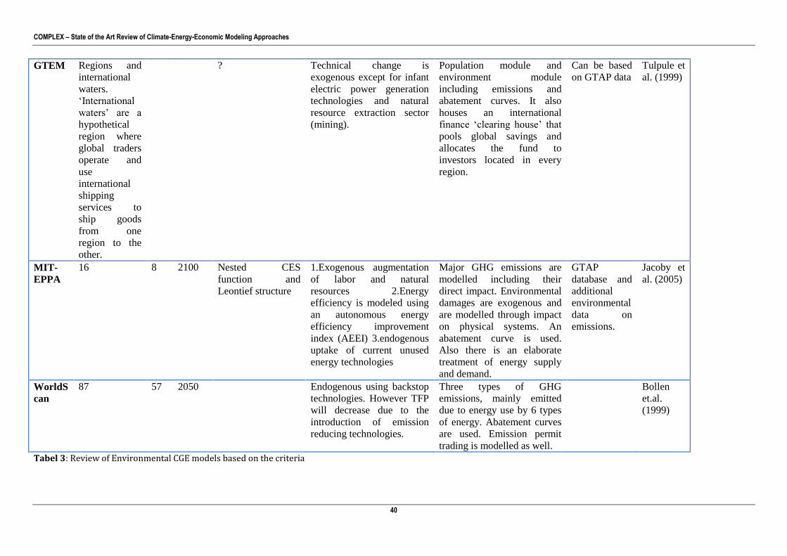
COMPLEX – State of the Art Review of Climate-Energy-Economic Modeling Approaches
40
GTEM Regions and
international
waters.
‘International
waters’ are a
hypothetical
region where
global traders
operate and
use
international
shipping
services to
ship goods
from one
region to the
other.
? Technical change is
exogenous except for infant
electric power generation
technologies and natural
resource extraction sector
(mining).
Population module and
environment module
including emissions and
abatement curves. It also
houses an international
finance ‘clearing house’ that
pools global savings and
allocates the fund to
investors located in every
region.
Can be based
on GTAP data
Tulpule et
al. (1999)
MIT-
EPPA
16 8 2100 Nested CES
function and
Leontief structure
1.Exogenous augmentation
of labor and natural
resources 2.Energy
efficiency is modeled using
an autonomous energy
efficiency improvement
index (AEEI) 3.endogenous
uptake of current unused
energy technologies
Major GHG emissions are
modelled including their
direct impact. Environmental
damages are exogenous and
are modelled through impact
on physical systems. An
abatement curve is used.
Also there is an elaborate
treatment of energy supply
and demand.
GTAP
database and
additional
environmental
data on
emissions.
Jacoby et
al. (2005)
WorldS
can
87 57 2050 Endogenous using backstop
technologies. However TFP
will decrease due to the
introduction of emission
reducing technologies.
Three types of GHG
emissions, mainly emitted
due to energy use by 6 types
of energy. Abatement curves
are used. Emission permit
trading is modelled as well.
Bollen
et.al.
(1999)
Tabel 3: Review of Environmental CGE models based on the criteria

COMPLEX – State of the Art Review of Climate-Energy-Economic Modeling Approaches
41
3.4 Discussion
There exist a vast number of CGE models dealing with environmental policy analysis. The models
reviewed here give a good overview of the existing environmental CGE models. The presented models in
this chapter have in common those they all are (recursive) dynamic and treat international trade such that
goods with the same statistical classification but different countries of origin are treated as non-perfect
substitutes. These presented models have been used in the literature for much policy analysis. The
disaggregation level differs a lot between the models reviewed in this chapter. The number of regions used
is between 8 and 113 and the number of production sectors goes from 7 to 200. In this review we looked at
one single-country model (AMIGA) and nine multi-country/global CGE models. Single-country models
tend to be more detailed in terms of sectors and household types, and they are in general used for analyses
of country-specific policy issues and proposals. Multi-country and global models, on the other hand, tend to
have less sector detail and to be designed for analysis of proposed multi-lateral policies such as free-trade
agreements. In the case of environmental CGE models the multi-country and global models in most cases
are designed for analysis of trans-boundary pollution problems.
Typically environmental CGE models have a time horizon of 2030 of 2050, but other such as the EPPA,
EXIOMOD and AMIGA have a time horizon of 2100. To capture effect of the policy change within the
model, the CGE models should incorporate several decades. Thus the development and implementation of
new technologies might affect emissions and other impacts on the environment much more than substitution
between currently existing technologies. There exists several ways to deal with deal with technological
changes in environmental CGE models. In AMIGA technology improvements are represented over time
(exogenously), and advanced technologies are included. EPPA models technical change in three ways. First,
there is an exogenous augmentation of the supplies of labor and natural resources. Second, energy use per
unit output decreases exogenously through time (the so-called autonomous energy efficiency improvement
index, or AEEI). The AEEI is a heuristic representation of non-price driven changes in energy use over
time. For developed countries there has been an observed improvement in energy intensity of the economy
that is not easily explained by fuel prices. While this improvement is sometimes considered due to technical
change, it can also result from changes in the structure of the economy. And third, included in EPPA are
energy technologies that are currently unused (or only at very small scale), but which come into play as
supplies of conventional energy resources deplete causing their prices to rise or as policies penalize the
GHG emissions of conventional fossil technologies. Their time of entry in a simulation depends on their
costs relative to those of current fuels, as they endogenously change in a forward simulation of EPPA.
GEM-E3 formulates production technologies in an endogenous manner allowing for price-driven derivation
of all intermediate consumption and the services from capital and labor.
In the electricity sector, the choice of production factors can be based on the explicit modeling of
technologies. In GTEM technological change is exogenous in GTEM. At the time of model application a
model user will have to decide what sort of technological change is to be assumed and apply that
accordingly. There are two areas in the economic core of GTEM in which technological changes are
endogenous. The first is infant electric power generation technologies, such as solar, are assumed to have a
‘learning by doing’ mechanism that lowers the primary factor input requirement per unit of output as
cumulative experience with the technologies grows. The second area is in the natural resource extraction
(mining) sector, where factor productivity declines with increases in the cumulative level of resource
extraction. Finally in WorldScan two developments in energy technology are important: more efficient use
of energy due to technological developments and increasing availability of new, economically viable energy
carriers, the so-called backstop technologies (also exists in GEM-E3 and EPPA).
Most reviewed models presented here make use of abatement cost functions (abatement curves) are used.
These can be seen as ad hoc rules to describe the trajectories of these emissions, following current
international modeling practice. There is no damage function in environmental CGE models that links
emissions growth to economic output through climate change or otherwise. Even if there is no direct
feedback from the environment module to the economic module, emission restriction policies will have
impacts on the economic module and hence, there is a strong link between the economic module and the
environment module.

COMPLEX – State of the Art Review of Climate-Energy-Economic Modeling Approaches
42
Appendix B: Environnemental CGE models
Model Institution Reference
AMIGA
(All-ModularIntegrated
GrowthAssessment Modeling
System)
Argonne National Laboratory, US;
Environmental ProtectionAgency
(EPA), US
Hanson and Laitner
(2004)
DART
(Dynamic Applied Regional Trade
Model)
Kiel Institute of WorldEconomics
(IfW), GermanyKlepper etal. (2003)
Klepper et al. (2003)
EPPA
(EmissionsProjection and Policy
Analysis Model)
Massachusetts Institute of Technology
(MIT), US
Jacoby et al. (2004)
EXIOMOD (Environmentally
eXtended Input-Output MODel)
TNO – Dutch Research Organization
for Applied Science
TNO
GEM-E3
(General Equilibrium Model fo
rEnergy– Economy–Environmen
tInteractions)
Catholic University of Leuven,
Belgium; NationalTechnical
University ofAthens, Greece; Center
for European Economic Research
(ZEW), Germany
Capros et al. (1998)
GEMINI–E3
(GeneralEquilibrium Model of
International National Interaction
for Economy– Energy–
Environment)
Ministry of Equipment, France;
Atomic Energy Agency, France;
University of Geneva, Switzerland
Bernard et al. (in
press)
G-Cubed
(Global General Eq. Growth
Model)
Australian Nationa lUniversity,
Australia; Syracuse University, US
Wilcoxen and
McKibbin (1999)
GTEM
(Global Trade andEnvironment
Model)
Australian Bureau of Agriculture and
Resources Economics (ABARE),
Australia
Tulpule et al. (1999)
WORLDSCAN Central Planning Bureau (CPB),
Netherlands
Bollen et al. (1999)
MIT-EPPA
(EmissionsProjection and Policy
Analysis Model)
Massachusetts Institute of Technology
(MIT), US
Jacoby et al. (2004)
Tabel 4: Reviewed Environmental CGE models
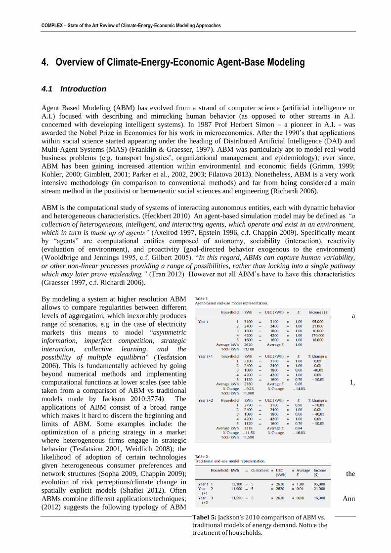
COMPLEX – State of the Art Review of Climate-Energy-Economic Modeling Approaches
43
4. Overview of Climate-Energy-Economic Agent-Base Modeling
4.1 Introduction
Agent Based Modeling (ABM) has evolved from a strand of computer science (artificial intelligence or
A.I.) focused with describing and mimicking human behavior (as opposed to other streams in A.I.
concerned with developing intelligent systems). In 1987 Prof Herbert Simon – a pioneer in A.I. - was
awarded the Nobel Prize in Economics for his work in microeconomics. After the 1990’s that applications
within social science started appearing under the heading of Distributed Artificial Intelligence (DAI) and
Multi-Agent Systems (MAS) (Franklin & Graesser, 1997). ABM was particularly apt to model real-world
business problems (e.g. transport logistics’, organizational management and epidemiology); ever since,
ABM has been gaining increased attention within environmental and economic fields (Grimm, 1999;
Kohler, 2000; Gimblett, 2001; Parker et al., 2002, 2003; Filatova 2013). Nonetheless, ABM is a very work
intensive methodology (in comparison to conventional methods) and far from being considered a main
stream method in the positivist or hermeneutic social sciences and engineering (Richardi 2006).
ABM is the computational study of systems of interacting autonomous entities, each with dynamic behavior
and heterogeneous characteristics. (Heckbert 2010) An agent-based simulation model may be defined as “a
collection of heterogeneous, intelligent, and interacting agents, which operate and exist in an environment,
which in turn is made up of agents” (Axelrod 1997, Epstein 1996, c.f. Chappin 2009). Specifically meant
by “agents” are computational entities composed of autonomy, sociability (interaction), reactivity
(evaluation of environment), and proactivity (goal-directed behavior exogenous to the environment)
(Wooldbrige and Jennings 1995, c.f. Gilbert 2005). “In this regard, ABMs can capture human variability,
or other non-linear processes providing a range of possibilities, rather than locking into a single pathway
which may later prove misleading.” (Tran 2012) However not all ABM’s have to have this characteristics
(Graesser 1997, c.f. Richardi 2006).
By modeling a system at higher resolution ABM
allows to compare regularities between different
levels of aggregation; which inexorably produces a
range of scenarios, e.g. in the case of electricity
markets this means to model “asymmetric
information, imperfect competition, strategic
interaction, collective learning, and the
possibility of multiple equilibria” (Tesfatsion
2006). This is fundamentally achieved by going
beyond numerical methods and implementing
computational functions at lower scales (see table 1,
taken from a comparison of ABM vs traditional
models made by Jackson 2010:3774) The
applications of ABM consist of a broad range
which makes it hard to discern the beginning and
limits of ABM. Some examples include: the
optimization of a pricing strategy in a market
where heterogeneous firms engage in strategic
behavior (Tesfatsion 2001, Weidlich 2008); the
likelihood of adoption of certain technologies
given heterogeneous consumer preferences and
network structures (Sopha 2009, Chappin 2009); the
evolution of risk perceptions/climate change in
spatially explicit models (Shafiei 2012). Often
ABMs combine different applications/techniques; Ann
(2012) suggests the following typology of ABM
Tabel 5: Jackson’s 2010 comparison of ABM vs. traditional models of energy demand. Notice the treatment of households.

COMPLEX – State of the Art Review of Climate-Energy-Economic Modeling Approaches
44
types based on their application and methodological approach:
1) Microeconomic models (e.g. ACE)
2) Space theory based models (e.g., GIS)
3) Psychosocial and cognitive models (e.g. TSi agents)
A. Actor-centered structuration theory (ST)
B. Integrative agent-centered (IAC) framework
C. Fuzzy cognitive maps (FCM)
D. Computational organization theory (networks)
4) Institution-based models
5) Experience- or preference-based decision models (rules of thumb)
6) Participatory agent-based modeling
7) Empirical- or heuristic rules (e.g. cluster analysis, econometric estimation)
8) Evolutionary programming
9) Assumption and/or calibration-based rules
4.2 Climate-Energy-Economic ABM review
UNESCO’s World Social Science Report of 2010 ( Kaldor 2010:11) makes a clear case, that research as
usual will not suffice to deal with the complexity of problems we face: “Global environmental change is a
challenge to traditional disciplinary research practices. The scale, rate, magnitude and significance of
changes to the global environment have made it clear that ‘research as usual’ will not suffice to help
individuals and groups understand and respond to the multiple, interacting changes that are now
occurring.” In the context of resource depletion, climate change and biological extinctions, ABM’s fills in a
very salient task: developing the capacity to realistically disaggregate highly abstract forecast scenarios
produced by other methods (e.g. what does global warming of 2 degree mean for Amsterdam, given
positive and negative social and environmental feedbacks?). In addition, to do this to a point where the
science can inform discrete and adaptive management strategies at the level where policies are
implemented. E.g. Balbi 2012.
Therefore, the application of ABM in this context promises to fill the gap between what is required and
what is possible for heterogeneous stakeholders in emergent contexts, e.g. between emission targets of the
EU and policy implementation details. (See Natarajan 2010, e.g. Balbi 2012) For example Jackson 2010
notes: “It is increasingly difficult to separate electricity use impacts of individual utility programs from the
impacts of increasingly stringent appliance and building efficiency standards, increasing electricity prices,
appliance manufacturer efficiency improvements, energy program interactions and other factors…Without
careful scrutiny, utility programs are prone to the same kinds of inefficiencies often found in other
programs designed to elicit certain consumer and firm responses”. We see the consequences of this failure
already in the analyses of existing climate change policies that for example do not analyze any
implementation details of particular policy instruments. Furthermore, there is a consistent and growing
‘emissions gap’ between the GHG reductions targets and the level scientifically correlated to stabilization
of the global climate. (den Elzen et al., 2011; Höhne et al., 2012; Kartha and Erickson, 2011; Rogelj et al.,
2011; UNEP, 2010b, 2011; c.f. Wiseman 2013) ABM therefore forwards the ultimate goal of
science/policy: which is to have the capacity to analyze strategies being forwarded (see Wiseman 2013 for a
meta-analysis) at a higher resolution; to do it within relevant time-frames; and to elaborate the specific
tactics of specific agents which will achieve specific targets. This requires a scalable and high fidelity
analysis of the non-linear transitions caused by purposive behavior of social agent/specific contexts vis-à-
vis the stochastic feedbacks of natural systems.
A case in point is the incapacity of current methods to study the effects of information provision, or of
exemplary reward and punishment. (Nannen 2010) Furthemore, Tol 2013 is the only one to do a cost
benefit analysis per EU country for the EU 20/20/2020 package, however the abatement cost might be
better informed if non-linearities in the climate, energy and economic system where included. ABM in this
context therefore means solving a complex strategic problem, without reducing it to a simple problem with
a single solution. It is not yet clear if ABM is the only method capable of doing this, but is one of with no

COMPLEX – State of the Art Review of Climate-Energy-Economic Modeling Approaches
45
intrinsic limitations to the task. Natarajan 2011 argues: “that a radically different, integrated, approach is
required to tackle these challenges and ensure that the modeling remains robust and able to meet future
demands. We suggest that Agent Based Modeling (ABM) is a suitable candidate modeling paradigm to
achieve an integrated modeling framework.”
In this review, it is clear that while there much advancement in the field there is only one application (Balbi
2013) that actually modeled emergent responses to climate change. However, this was done for Alpine
Tourism, which is only a small part of one of many sectors, which are of relevance. Other models that deal
with feedbacks across systems do so in very stylized way (Gerst 2012), e.g. homogenous demand, of
homogenous goods and stylized electricity types. ABM’s that deal with MBI such a emissions trading
(Chappin 2012, Weidlich 2013, Sun 2007, Bunn 2007), focus on the supply side and on markets
specifically, which means they do not treat climate or energy demand in a dynamic and adaptive way. In
fact no model reviewed here treats climate as a complex adaptive system or even dynamically. Furthermore
there is a lot of ambiguity in terms of both validation and treatment of the model outputs. In both regards,
there are also specific attempts to fix these issues (Muller 2013 and Gerst 2012 respectively). It is also
evident that the development of a model which can address all these issues vis-à-vis be formulated and
applied in a way which is of relevance to the stakeholders is not an easy task.
4.2.1 General review aspects
The application of ABM models to climate-economy-energy systems reviewed here consisted mostly of
microeconomic, empirical- or heuristic rules, evolutionary programming and assumption and/or calibration-
based rules. Most cases at most consist of one link with descriptive reference to another system, e.g.
Economy-to-energy: economic cost of stylized energy types based on their GHG emission profiles.
Indigenizing energy economy and environment feedbacks with robust representations of each respective
system (integrative modeling of EEC systems) is clearly yet to achieved within ABM, e.g. modeling
(micro) economy-to-energy-to-climate-to-economy. There is also a general ambiguity in terms of justifying
the numbers of agents, integration step, time period, validation technique and treatment of simulation
outputs; all these apparent flaws or lack of methodological rigor are however often justified in terms of the
ABM’s purpose, and i.e. the quality of an ABM depends on the application or formulation of the problem.
In general terms however it is clear that much of the promise or potential of ABM’s to address the scientific
gaps in energy-economy-climate systems has yet to be realized. Only one ABM (Balbi 2013) actually
modeled emergent responses to climate change. However this was done for Alpine Tourism, which is only a
small part of one of many sectors which are of relevance.
MICROECONOMIC ABM
GER
ST 2
01
2
WEI
DLI
CH
20
08
KEM
PEN
ER 2
00
9
SOP
HA
20
13
NA
NN
EN 2
01
2
SUN
20
07
NIC
OLA
ISEN
20
01
CH
AP
PIN
20
09
CH
AP
PIN
20
12
TRA
N 2
01
2
WIT
TMA
NN
20
06
BU
NN
20
01
LI 2
01
2
SHA
FIEI
20
12
DEI
SSEN
BER
G 2
00
8
BA
LBI 2
01
3
NA
TAR
AJ
20
11
ZHA
NG
20
13
MA
TSU
MO
TO 2
00
8
JAC
KSO
N 2
01
0
ABM TYPE
SPACE THEORY BASED ABM
EVOLUTIONARY PROGRAMMING ABM
EMPIRICAL OR HEURISTIC RULE ABM
ASSUMPTION AND/OR CALIBRATION-BASED ABM
PSYCHOSOCIAL OR COGNITIVE ABM
PARTICIPATORY ABM
INSTITUTION BASED ABM
Tabel 6: Overview of ABM models over ABM types . * = strong level of correlation, =correlation

COMPLEX – State of the Art Review of Climate-Energy-Economic Modeling Approaches
46
1) Link between climate and energy
The application of the ABM is often nested in a larger system. This larger system is often treated
differently; therefore it is crucial to understand the link and order between subject-to-subject (energy,
climate, economy). This is necessary as in ABM, often one part of the model is treated as a complex
adaptive system and the part(s) of the model are simplified (treated the same as in GE, SD, e.g. single
representative agents or stocks). Furthermore it is necessary to understand what type of link or feedback
there is between the two (see 1.4.5.A Feedback Type). The order of integration (or hierarchy, within one
step), the treatment of subsystems and the type of link (signal passing or passing of a complex data
structure31
) have non-marginal implications in the outputs of the model. There are no comparative
sensibility studies done in this regard, so it is hard to draw conclusions or discern clear patterns. None of the
ABM’s reviewed here, expects for Balbi 2013, went beyond representing two links (see Figure 6 ). A
majority focuses on economic and/or energy and none model climate-to-climate links (e.g. fluctuation in
ecosystem services as a result of climate change).
Economy-to-
climate
E
C E €
C
€
Energy-to- climate
E
C E €
C
€
Climate-to-
climate
E
C E €
C
€
Economy-to-
energy
E
C E €
C
€
Energy-to-energy
E
C E €
C
€
Climate-to-
energy
E
C E €
C
€
Economy-to-
economy
E
C E €
C
€
Energy-to-
economy
E
C E €
C
€
Climate-to-
economy
E
C E €
C
€
Tabel 7: matrix of link types between systems per run step
GER
ST 2
01
2
WEI
DLI
CH
20
08
KEM
PEN
ER 2
00
9
SOP
HA
20
13
NA
NN
EN 2
01
2
SUN
20
07
NIC
OLA
ISEN
20
01
CH
AP
PIN
20
09
CH
AP
PIN
20
12
TRA
N 2
01
2
WIT
TMA
NN
20
06
BU
NN
20
01
LI 2
01
2
SHA
FIEI
20
12
DEI
SSEN
BER
G 2
00
8
BA
LBI 2
01
3
NA
TAR
AJ
20
11
ZHA
NG
20
13
MA
TSU
MO
TO 2
00
8
JAC
KSO
N 2
01
0
ABM TYPE
ECONOMY-TO-ENERGY
ECONOMY-TO-CLIMATE
ECONOMY-TO-ECONOMY
ENERGY-TO-CLIMATE
ENERGY-TO-ENERGY
ENERGY-TO-ECONOMY
CLIMATE-TO-CLIMATE
CLIMATE-TO-ENERGY
CLIMATE-TO-ECONOMY
LINK
Figure 6: Overview of ABM models over LINK TYPES. * = strong level of correlation, =correlation
31 Signal passing is the passing of a variable state, there can also be a interaction where a complex data structure is passed which would consist of a series of structured variable states (i.e. a structured composition of letters or numbers).

COMPLEX – State of the Art Review of Climate-Energy-Economic Modeling Approaches
47
2) Mitigation Strategies
There are two type of mitigation strategies, the ABM models reviewed here did not focus on command and
control instruments (e.g. 1987 Montreal Protocol) but instead focus on the following market-based
instruments (MBI): cap and trade (CT); public research and development expenditures; and taxes. MBI that
were not modeled include: voluntary green power programs; renewable portfolio standards and quotas;
tendering; net metering; system benefits charges, and; tradable certificates and guarantees of origin (all
which are policy instruments often considered, by the European Energy Agency (see McEency 2013)).
There are also a broad range of theoretical mitigation strategies that could be considered but where not.
3) Non-linear or emergent responses to climate change The only ABM explicitly model a non-linear response to climate change, meaning was able to model
emergent behavior in response to climate change was Balbi 2013. It should be said however that here are
many definitions of non-linearities, often the terms is equivalent to emergent phenomena. “Emergent
phenomena result from the interactions of individual entities. By definition, they cannot be reduced to the
system's parts: the whole is more than the sum of its parts because of the interactions between the
parts.”(Bonabeau 2000). Non-linearities are often manifest when a model has thresholds, irreversibility and
non-linearities (non-linear inputs and/or implementation, resulting in non-linear outputs) which we describe
in the table per ABM. However that an ABM may have all three qualities doesn’t not necessarily mean that
it captures emergent behavior; since it is fundamentally a question to which degree are these features
affecting the model outputs. All ABM reviewed here have non-linearity and irreversibilities but none had
thresholds in the output (clear bifurcations into stable states).
As Tabel 8 shows, having these qualities will not necessarily produce any non-linear response at any level
(see Tabel 8 for an explanation on these relationships), i.e. a model can have non-linear inputs and non-
linear implantation and still produce no emergent or non-linear response. In the end it is a matter of to
which degree and which part of the model is non-linear; to this effect however we see that very few ABM’s
run sensibility analysis on the adaptive traits of the agents (some exception being: Weidlich 2008, Chappin
2012, Sopha 2013). Furthermore it should be noted that there is a tradeoff between models capacity to
represent emergent behavior and that models capacity to be validated empirically. In this regard ABM
provides a way to mitigate but not solve the practical problem that is a lack of good data and limits of
individual researchers. In the context of non-linear responses to climate change, we see of course very few
sources of good data, which result in either an ad-hoc or experimental parameterization of such responses.
It should also be noted that while ABM is the best method to model non-linearities or emergent behavior,
the fact remains that unless there is a high level multi-threading interface32
or event based hierarchy in the
end, an ABM -as complex as it may be- will effectively run like a linear program, e.g. System Dynamics or
Spatial Econometrics. From the ABM’s reviewed here, we see that the models are sensitive to prices more
than to implementations of bounded rationality or expectation formations.
32 Multi-threading is a widespread programming and execution model that allows multiple threads (functions) to exist within the context of a single process (time step). These threads share the process' resources, but are able to execute independently.
Tabel 8: relationship between data, ABM implementation, outputs and emergent behavior
Non-linear Inputs + Non-linear Implementation +
Non-linear Outputs = Emergent behaviour?
x x x x x x x
x x
Threshold(s) in Inputs+
Threshold(s) in Implementation+
Threshold(s) in Outputs=
x x x

COMPLEX – State of the Art Review of Climate-Energy-Economic Modeling Approaches
48
4) Nonlinearity, threshold and irreversibility
All of the ABM’s reviewed here are non-linear in their implementation, but only Balbi 2012 models a non-
linear or emergent response to climate change. None of the ABM models reviewed here had explicit
thresholds (at a global level, i.e. outside of the agent). However most learning algorithms function by using
a updating a threshold/function related to the mix, max or average of previous state variables; but this
should not be considered, as it is fundamentally a technique to model memory or strategic behavior of
agents, more than a technique to model a non-linearity or power law.
All ABMs are allow for irreversibility, in that the model has at least two elements (agents) whose parameter
space or behavior is locked-in, path dependent and process specific. Therefore the sequence of previous
states constraint future states.
5) Technological development
No ABM reviewed here included endogenous technological development. Meaning that no ABM reviewed
here has modeled an explicit mechanism and/or dynamics for technological innovation. However, some
ABM model investment and divestment into stylized electricity production technologies, e.g. Gerst,
Chappin 2012. Other ABM’s model transitions in terms of market share of theoretical technologies such as
Clean Coal, e.g. Chappin 2009. Other ABM’s model technological end-use and market-share forecasts, e.g.
Sopha 2013, Shafiei 2012, and Nannen 2010.
6) Feedback mechanisms
Subsystem
reference or
link / Step
System-to-
system link /
Step
Two-System-to-
system link / Step
n-order Feedback /
Step
Exempel:
Economy-to-
economy
Economy-to-
climate
Economy-to-
economy-to-climate
Economy-to-
economy-to-energy-
to-energy
Figure 7: feedback types
x x x x
x x
Irreversibility in Inputs +
Irreversibility in Implementation +
Irreversibility in Outputs =
x x x x x x x
x x

COMPLEX – State of the Art Review of Climate-Energy-Economic Modeling Approaches
49
Most ABMs reviewed here consist of a subsystem reference (e.g., economy-to-economy or energy-to-
energy and none had explicit 2nd
order feedbacks33
(while sometimes the aggregated distributions show
evidence that it is in all a second order system, e.g. Balbi 2013). Only one ABM reviewed here had
feedbacks consisting of more than signal passing. Deissenber (2008) was the only ABM in which the
feedback is a complex data structure or string. None of the ABM’s reviewed endogenized all three systems
(energy, economy and climate) as complex adaptive systems. In most cases climate systems where treated
only in terms of reference or heterogeneity within the economic and energy sector, e.g. preferences for
carbon heavy, carbon light, carbon free. No ABM modeled the climate as an agent -in the ABM tradition-
or even modeled different scenarios based on climate change scenarios (again except for Balbi 2013). No
ABM modeled positive feedbacks in climate change.
GER
ST 2
01
2
WEI
DLI
CH
20
08
KEM
PEN
ER 2
00
9
SOP
HA
20
13
NA
NN
EN 2
01
2
SUN
20
07
NIC
OLA
ISEN
20
01
CH
AP
PIN
20
09
CH
AP
PIN
20
12
TRA
N 2
01
2
WIT
TMA
NN
20
06
BU
NN
20
01
LI 2
01
2
SHA
FIEI
20
12
DEI
SSEN
BER
G 2
00
8
BA
LBI 2
01
3
NA
TAR
AJ
20
11
ZHA
NG
20
13
MA
TSU
MO
TO 2
00
8
JAC
KSO
N 2
01
0
LINK OR FEEDBACK TYPE
SYSTEM- TO- SYSTEM LINK
SUBSYSTEM REFERENCE OR LINK
TWO SYSTEM-TO-SYSTEM LINKS
N-ORDER FEEDBACK
Figure 8: Summary per ABM of link or feedback type
7) Representation of the key economic sectors
The majority of the ABMs reviewed here deal with either the electricity, technology or end use of
electricity and technology from an economic Perspective (Gerst 2012, Weidlich 2008, Sopha 2013,
Kempener 2009, Nannen 2012, Sun 2007, Nicolaisen 2011, Chappin 2009, 2012, Tran 2012, Wittmann,
Brunn 2001, Zhang 2011, Matsumoto 2008, Jackson 2010, Natarajan 2011). Tran 2012 and Shafei 2012
deal with wholesale and retail of motor vehicles. One model deals with tourism (Balbi 2012) and a couple
are macroeconomic (representing more than one sector at a national or EU level) (Deissenberg 2008 and
Gerst 2012). Deissenberg 2008 while claiming to have model the whole economy, only presents results
from employment dynamics (searching for and hiring of employees). Natarajan 2011 models energy
consumption and emission based on construction of households.
8) Representation of energy sources
There is a difference between energy and electricity. For example the energy consumption of a household
could include food and electricity consumption could not. The majority of the ABMs reviewed here given
that ABMs often deal with future events, focus on electricity production and do so in a stylized manner. For
example Gerst 2012 treats electricity as ‘carbon-heavy’, ‘carbon-light’, and ‘carbon-free’, each with a
respective cost and for which agents will have specific utility and welfare functions. This is the case as there
is no data on what new technologies could produce and at what cost. However, some models endogenize the
theoretical parameters of non-existent technologies and parameterize them with projections, e.g. clean coal /
Chappin 2012. Some authors who do not produce forecasts, use vintage data to represent the energy
generation of for example wind mills, which is highly variable (Li 2012). From which they make inferences
about the market structure / MBI’s. Tran 2012 and Shafei 2012, given that they are doing technology
market share forecasting of motor vehicles parameterize their models at a higher resolution and use
multicriterion optimization. ABM’s concerned with end-use of appliances such as Sopha 2012 also
parameterizes their models with higher resolution.
33 A feedback of a feedback or second order derivative, e.g. a state triggers a signal from the economic system to the energy system, which in turns triggers a response in climate system.

COMPLEX – State of the Art Review of Climate-Energy-Economic Modeling Approaches
50
9) Spatial Scales
19
8 1 10
4 4 -6 3 7
MESO LEVEL
MICRO
LEVEL
MACRO LEVEL
Figure 9: Scale resolution. This distinction is valuable as ignoring the variance of a variable especially in discrete systems could result in erroneous estimations. Therefore it is most desirable to model a system from the lowest (micro) to the highest (macro) level of aggregation.
Micro-meso-macro Meso-
macro
Micro-meso Macro-micro Macro
The utility of ABM is often in disaggregating a particular spatial or temporal scale. For example taking
available data on electricity production, market structure and transaction prices and developing an ABM to
model the microeconomic behavior of the firms involved (Weidlich 2008). This is valuable as ignoring the
variance of a variable especially in discrete systems could result in erroneous estimations. This point was
made in economics by Anscombe (1973) and well understood in mathematics and natural science’s
concerned with modeling. However many ABM reviewed here does not have this variance in scale, but
model a particular instance. Below you see Anscombe’s Quartet (cf. Tabel 9 and Figure 10: Anscombe’s
Quartet (1973) , there is a graphical description of possible spatial domains. The actual borders of the model
domain or environment (mix, max, and sector) are specific to the author, i.e. what is macro or micro is
determined by the author or rather is not general but ABM case specific. Notice in Tabel 9 and Figure 10,
the disaggregation of the patterns from macro to micro.

COMPLEX – State of the Art Review of Climate-Energy-Economic Modeling Approaches
51
y = 0.5001x + 3.0001 R² = 0.6665
0
2
4
6
8
10
12
0 5 10 15
y = 0.5x + 3.0009 R² = 0.6662
0
2
4
6
8
10
12
0 5 10 15
y = 0.4997x + 3.0025 R² = 0.6663
0
5
10
15
0 5 10 15
y = 0.4999x + 3.0017 R² = 0.6667
0
2
4
6
8
10
12
14
0 5 10 15 20
SET A: X1=[10 8 13 9 11 14 6
4 12 7 5];
SET B: X2=[10 8 13 9 11 14 6
4 12 7 5];
SET C: X3=[10 8 13 9 11 14 6
4 12 7 5];
SET D: X4=[8 8 8 8 8 8 8 19 8
8 8];
Y1=[8.04 6.95 7.58 8.81 8.33 9.96 7.24 4.26 10.84
4.82 5.68];
Y2=[9.14 8.14 8.74 8.77 9.26 8.1 6.13 3.1 9.13 7.26
4.74];
Y3=[7.46 6.77 12.74 7.11 7.81 8.84 6.08 5.39 8.15
6.42 5.73];
Y4=[6.58 5.76 7.71 8.84 8.47 7.04 5.25 12.5 5.56 7.91
6.89]; Tabel 9: Anscombe’s Quartet (1973) dataset
All the mean of the x values = 9.0
All the mean of the y values = 7.5
All the least-squared regressions are: y =
0.5 x + 3
All the sums of squared errors (about the
mean) = 110.0
All regression sums of squared errors
(variance accounted for by x) = 27.5
All residual sums of squared errors
(about the regression line) = 13.75
All the correlaten coefficient = 0.82
All coefficient of determination = 0.67
In Anscombe’s Quartet (1973) we see that different
data sets result in the same correlation, error, and
linear trajectory, yet clearly they are differences, i.e.,
statistical methods have intrinsic limitations as a
proxy for estimating the validity of even linear
systems. This means that there could be hundreds of
parameter variations of a model derived solely from
statistical rigor/metrics; and that deciding the
validity of model would base solely on this would
not be enough. This means that it is impossible to
validate or falsify a discrete and dynamic system
with statistical methods/vintage data set
(quantitative empiricism) alone. Conversely it is
rather simple to statistically fit a model to any data
set. This explains why the capacity for flexibility
and micro level foundations of ABM is of particular
interest for integrated EEC models. Table 5 in the
next page summarized the spatial domains per
article. Ideally an ABM capable of modeling micro-
meso-macro would be preferred.
Figure 10: Anscombe’s Quartet (1973)

COMPLEX – State of the Art Review of Climate-Energy-Economic Modeling Approaches
52
Tabel 10: Summary of ABM spatial scales
Micro-meso-
macro
Meso-macro Micro-meso Macro-micro Micro
Author
Gerst 2012 x
Weidlich 2008 x
Sopha 2013 x
Kempener 2009 x
Nannen 2012 x
Sun 2007 x
Nicolaisen 2001 x
Chappin 2009 x
Chappin 2012 x
Tran 2012 x
Wittmann 2006 x
Bunn 2001 x
Li 2012 x
Shafei 2012 x
Deissenberg 2008 x
Balbi 2013 x
Nataraj 2011 x
Zhang 2013 x
Matsumoto 2008 x
Jackson 2010 x
10) Time scales
There is a huge amount of variance in the ABM applications, ranging from hourly to yearly, from 31 steps
to 4000. The time range is often an ad-hoc choice which no author so far has cared to justify. Therefore,
there is no discernible rigor or patterns in this regard. There is also no sensibility analysis applied to the
integration sequence-order. Unlike regression models, the quality of an ABM model will not necessarily
dependent on the amount of data used. Furthermore, for both ABM and regression models having too many
integration steps, will result in a loss of numerical precision given the computational limitations of current
computers (16-64 bits). This is perhaps why no authors care to justify the integration step or scale; in that it
is may well be a more complex problem to formulate and solve that the problem at hand. For example it
would require that the model be implemented in different computers and software’s. Such level of
replication is basically non-existent in either conventional or ABM. One possible pattern in the literature is
that microeconomic models and specifically those of the ACE tradition might limit the time domain and
scale to the availability of data from electricity production and transaction prices. They do this in order to
estimate the effect of strategic behavior and market structure. For the rest of ABM’s there is no clear
relationship between the time scale and quality or application domain.
12) Representation of Market
ABM which follow the Agent-Based Computational Economics (ACE) tradition (Weidlich 2008 Nicolaisen
et al. 2000, 2001, Lane et al. 2000, Bunn and Oliveira 2001, 2003, Bower and Bunn 200, 2001, Bower et al.
2001, Bunn and Oliveira 2006, Visudhiphan and Llie 2002, Sun and Tesfatsion 2007, Ruperes, Michola et.
Al 2004, Cincotti et. Al 2006, Weidlich and Veit 2006, Krause et al 2005,Naghibi-Sistani et al. 2006, Xiong
et al. 2004, Bakirtzis and Tellidou 2006,) model electricity market as a complex adaptive system. Most

COMPLEX – State of the Art Review of Climate-Energy-Economic Modeling Approaches
53
other ABM’s who do not, if the market is modeled at all will have one side of the supply or demand drive
the other without any clearing mechanism or transaction control or constraints.
11) Representation of demand and supply in energy market
Most ABM’s reviewed here are focused in the representation of electricity production, in which demand or
actual transaction data is used as a static or empirical variable. However we also see in Gerst 2012 a
representation of demand which is endogenously driven by socioeconomic conditions. However, in Gerst
2012 demand is not represented as heterogeneous agents but as homogenous function of employment (Total
Household Normalized Energy Expenditure Division (‘thneed’) (Geisel, 1971). Other ABM which model
energy demand do so in a narrow sense, e.g. modeling the end use of energy based on office management
and technology (Zhang 2013); or end use of heating appliances in Norway (Sopha 2013). While current
ABM forward the capacity toward modeling energy consumption behavior. There is a clear gap of the
ABMs in their modeling systems (non-linear negative feedbacks in response to climate change) at any rate
that might be relevant for environmental public policy. For example: what kind of system flip can we
expect from changes in a sector which is less 4.5%-9% of total energy consumption/GHG (household
electricity use); of which appliances are less than 15% of household energy consumption; and whose
efficiencies with green appliances might at best be at best 20%-80% in the next 40 years. Clearly less than
one percent aggregate change in the best scenario. Fisher and Irvine 2010 empirically document the level
of reductions in electricity, gas, water and waste achieved at the household level by different groups (British
and Dutch ECO teams, Grag’s and Green Streets). In order to model emergent or non-linear responses to
climate change it is clear that an ABM would have to be applied in a nature similar to the work of Fisher
and Irvine 2010 in a way that is relevant to policies being proposed (Wiseman 2013).
The supply of energy is presented in various ways, Weidlich 2008, present the most robust model however
it is still for an analysis of a specific process. Weidlich 2008 as well as Bunn and Oliveira 2006, Li 2012,
and Sun and Tesfatsion 2007 all focus on the strategic behavior of liberalized energy markets. Gerst 2012
and Chapin 2009 model investment and divestment in electricity generation technologies. No ABM has
modeled the electricity technologies with dynamic values over time, this would be relevant as most ABM
deal with forecasting future trends. Therefore there would be value in informing the Energy Invested on
Energy Returned (EIOER) ratios vis-à-vis projection in terms of end-use efficiency in the representation of
electricity supply.
12) Validation
Amid clear attempt to standardize ABM model verification (“ODD Protocol for Describing Three Agent-
Based Social Simulation Models”34
, Volker Grimm et al. 2006, and “Describing human decisions in agent-
based models – ODD + D, an extension of the ODD protocol”35
Muller 2013). In the ABM reviewed here
there is absolute ambiguity in terms how to treat the outputs of the models, e.g. should the outputs of a
specific scenario be averaged, or picked, or should cluster analysis be implemented to discover scenarios
(Gerst 2012), or should there some kind of process listener-control at run time, etc. There is also ambiguity
in terms of what “sensitivity analysis” means, e.g. random seed variation, or temporal model variation, or
variation in the level of data aggregation, or variation of sample size, or variation in the decision processes
and capabilities of the agents, etc. (Richardi 2006). There is also no standard in terms of the integration
period, sequence, range, etc. which has severe implications given the finite precision of computers
(McCullough 2009:53). So it is often a series of ad hoc choices with non-marginal results that constrain the
complexity/application of ABMs. It is for this reasons that most ABMs often do not stray too far from the
minimalism problem formulation /application of conventional models, e.g. Nannen 2010. However this
limitations are a sign of the relative novelty of ABM and not precluding factor of ABMs capacity.
Most ABM’s have at least one subsystem parameters derived from empirical data. Some had several parts
of the ABM informed by a combination of survey data, empirical data, secondary data, panel data, or
experimental data. Given the large domain that ABMs cover, it is almost impossible to expect that every
parameter and function in a ABM is derived from empirically validated data; ABM is an exploratory not
descriptive technique. In fact ABM that constrain the functions and parameters of the agents exclusively to
empirical data, often results in very static models (e.g., Sopha 2013).
34 http://www.sciencedirect.com/science/article/pii/S030438001000414X 35 http://www.sciencedirect.com/science/article/pii/S1364815213001394

COMPLEX – State of the Art Review of Climate-Energy-Economic Modeling Approaches
54
4.2.2 ABM specific review aspects
1) Theoretical framework for agents behavior
ABM in itself presents a theoretical and epistemological paradigm, which fundamentally aims to represent a
complex system in as much detail as possible. This is not always the case for other methodologies applied
in the same context. Beyond this, there is a huge variance in terms of which specific theories the author’s
use to justify the epistemological and methodological choices. For example Gerst 2012 bases his ABM on
the work of the DRF model by Dosi, Fagiolo et al. (2010). This model is then based on Schumpeter’s
business cycles, and adds a simplified energy system (3 types of energy based on their emission profiles) .
Other ABM’s use more general theoretical frameworks such as Wittmann 2006 who uses Social Miliues
(SINUS-Milieu-Typology ) and rationality types. Sopha 2013 uses Theory of Planned Behavior, Diffusion
of Innovation Theory, Meta-Theory of Planned Behavior, Utility Theory. Most other authors do not frame
their ABM within a theoretical framework but simply disclose the interaction structure and sequence, which
in itself is a theory.
2) Heterogeneity
Most ABM’s have heterogeneity in terms of the initial and run time state parameters of at least one class of
agents. However, this is not true for all ABM’s; in Diessenberg 2008, all agents consist of two states and
only two agent classes. However, the Authors do not describe what the transition functions are so it is hard
to draw conclusion about their ABM. Most ABM’s will have more than one type of agents treated within
the ABM tradition, however it is also the case that ABM’s will sometimes use representative agents to
model climate, ISO, Demand or governments.
3) Bounded Rationality Bounded rationality is a hypothesis: “rational agents experience limits in formulating and solving complex
problems and in processing (receiving, storing, retrieving, transmitting) information". (Simon 1957) These
include: limiting the types of utility functions, recognizing the costs of gathering and processing
information, and possibility of having a "vector" or "multi-valued" utility function.
All ABM’s implement bounded rationality through an internal maximization function, the rest use of both
behavior satisfaction and maximization (Wittmann 2006). The later means that the internal maximization is
activated by a response to another agent or environment. That is to say that bounded rationality is limited by
the heterogeneous characteristic/functions of the agents. It would be very hard to call a ABM an ABM
without a clear implementation of bounded rationality. In the case of Agent-Based Computational
Economics (ACE) tradition or microeconomic ABM’s (Weidlich 2008 Nicolaisen et al. 2000, 2001, Lane et
al. 2000, Bunn and Oliveira 2001, 2003, Bower and Bunn 200, 2001, Bower et al. 2001, Bunn and Oliveira
2006, Visudhiphan and Llie 2002, Sun and Tesfatsion 2007, Ruperes, Michola et. Al 2004, Cincotti et. Al
2006, Weidlich and Veit 2006, Krause et al 2005,Naghibi-Sistani et al. 2006, Xiong et al. 2004, Bakirtzis
and Tellidou 2006,) we see the rationality of the agents is constrained internally, and further by the ISO
which clears the market. Only one ABM consisted of only purely behavior satisfaction (Diessenberg 2008).
4) Adaptive expectation formation
Adaptive expectation formation is commonly implemented through a learning algorithm. For example this
will be implemented in a way that each agent is assigned one out of a number strategies for setting their
response (e.g. bidding or buying). Specifically: These can be set equal to (i) the maximum, (ii) the mean, or
(iii) the minimum of historic prices, to (iv) the sum of weighted historic prices, (v) the last bid price plus the
difference between the last market price and the last bid price, weighted by a constant β, or to (vi) a target
price plus the absolute value of the difference between the last market price and this target price, weighted
by a constant β; the value of β depends on the success in the previous round.“ (Weidlich 2008)
Weilich 2008 and Sopha 2008 are the only ABM’s reviewed here to have sensibility analysis or a
comparison of different types of adaptive expectation formations. Specifically Weidlich 2008 compares
reinforced learning: Erev & Roth and Q-learning algorithms. Sopha 2008 compares small world networks
and random networks. Evolutionary algorithm’s is another technique used to represent and agents adaptive
response to and environment as well as mutation, e.g. Nannen 2010. Chappin 2012, implements what he
calls a memetic function as well as network influence.

COMPLEX – State of the Art Review of Climate-Energy-Economic Modeling Approaches
55
5) Interaction
Wittmann 2002006 is the only ABM to have a variation of interaction hierarchies. His ABM is
implemented in an operational, structural and scenario hierarchy. Diessenberg 2008 is the only ABM to
have a purely event driven interaction hierarchy. For the rest of the ABM the interaction is fundamentally
linear, i.e. arranged by the order of computation between the agents and the state variables, e.g. Chappin
2009: update exogenous scenario parameters electricity trading emission trading fuel trading
investment and divestment. It is also important to understand the ABM’s output will be sensitive to the
interaction sequence/implementation. However, no ABM has so far done sensitivity analysis by variation of
the interaction structure, which would clear value to the discipline.
6) Macro Metric Output
There is a huge range in terms of the metrics used, however the one discernible pattern is that none of the
ABMs reviewed here treated emissions from economic activity or energy consumption beyond stylized
ways, i.e. no ABM here had methane + CO2 + particles, etc. The lack of such metrics for which there is
ample data elucidates the fact that he feedbacks between economic/energy systems and climate systems are
very weak. It could also be said that perhaps the representation of climate at a higher fidelity would add no
analytical value to the comparison of MBI’s. However no author justifies this point.
1.4.10.C) Structural Validation? (ABM specific criterion)
Very few ABMs perform some kind of Structural validation. When it is performed, it is only for one aspect
of the model (e.g. energy generation, in an energy market). ABMs are in theory capable of having a 1:1
ratio of data granularity, e.g. each survey or data point, can be represented fully as an aspect on an agent’s
heterogeneity. However it is often the case that ABM’s actually go beyond that and produce experimental
data which cannot be validated in any rigorous way.
7) Statistical Test
There is a broad range of statistical test perform as well as a large number of ABM’s which do not perform
any at all. Chappin 2009, 2012 is the only author to perform test in reference to the complexity science
literature. However the results are not explicit in the paper. Some authors apply Monte Carlo methods and
others (Gest 2012) suggest cluster analysis as a scenario discovery tool. There is allot of variance in terms
of what tests are necessary to validate the model and further where in the ABM should this test be
implemented. For example Sopha 2012 validated the input parameters, others restrict the run state constants
to empirical data (Weidlich 2008), and other compare the outputs of the ABM with the empirical data
(structural validation).
8) Sensitivity analysis
Almost all ABM that are developed with high level programing languages (e.g., Net Logo, Anylogic,
Repast) will be developed vis-à-vis a graphic user interface that allows for the variation of initial
parameters. However there is absolute ambiguity as established by Richardi (2006) in terms of how and
where in the ABM to perform sensibility analysis. Richardi 2006 elaborates: “”…the term is currently used
as a general catch all for diverse techniques: there is no precise definition and no special methodology
currently associated with this term. We define sensitivity analysis as a collection of tools and methods used
for investigating how sensitive the output values of a model are to changes in the input values (see Chattoe
et a. 2000). A "good" simulation model (or a "significant" result) is believed to occur when the output
values of interest remain within an interval (which has to be defined ), despite "significant" changes in the
input values (which also have to be defined).”
9) United Modeling Language Diagram (UML)
Most ABM come with some sort of descriptive diagram. Weidlich 2012, Chappin 2012, Balbi 2013, Shafiei
2012, Deissenberg 2008, Zhang 2013 had a UML diagram. In the next page there are two types of UML
(class and sequence) from Weidlich 2008. The UML diagrams when done properly can easily explain
complex interaction and class structures.
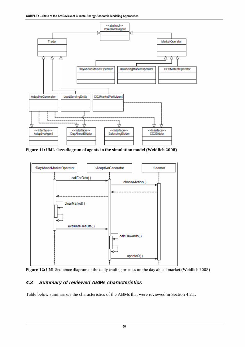
COMPLEX – State of the Art Review of Climate-Energy-Economic Modeling Approaches
56
Figure 11: UML class diagram of agents in the simulation model (Weidlich 2008)
Figure 12: UML Sequence diagram of the daily trading process on the day ahead market (Weidlich 2008)
4.3 Summary of reviewed ABMs characteristics
Table below summarizes the characteristics of the ABMs that were reviewed in Section 4.2.1.

COMPLEX – State of the Art Review of Climate-Energy-Economic Modeling Approaches
57
Author, year
1. A) Issues?
2. A) Links Between Climate And Energy? B) MBI?
3. A) Non-Linearity? 3. B) Thresholds, 3.C) Irreversibility?
4. A) Endogenous Tech Development?
5. A) Feedback or link Type?
6. A) Econ Sectors? B) Energy Sources?
7. A.) Spatial Scales? 10. B) Time Scales?
8.Representation of A) Demand B) Supply C) Market
9. Agent Design A)Theory B)Heterogeneity C)Bounded Rationality D)Expectation Formation E)Interaction
10. A) Empirical Parameterization? B)Macro Metric Output C) Structural Validation? D) Statistical Test? E) Sensitivity analysis? f) UML?
Gerst 2012
Proof of concept, ABM for scenario discovery and discovery of enhancing or retarding factors of policy. Microeconomic models
E
C E €
C
€
A)Stylized energy types B) NO C) BAU, Tax, R&D, Tax+R&D and R&D Shift
3. no emergent response to climate change A) yes B) no C) yes
A) No ECONO
MYENERGY PRODUCTION ENERGY CONSUMPTION. Signal passing.
A) Energy B) three stylized energy technologies: ‘carbon-heavy’, ‘carbon-light’, and ‘carbon-free’
A)MICRO (level 1),MACRO/ Based on Putnam (1988) two-level game. For spatial domain reference to Nordhous (2008) and Sissine (2011) B) 50 simulations 1 step per year: 2000 to 2300
A)Static/ Total Household Normalized Energy Expenditure Division (‘thneed’) (Geisel, 1971). demand of homogenous capital goods, consumer goods, laborers-consumers B) different investment rules based on energy carbon heavy, carbon light and carbon free C) No market clearing mechanism, income from
A) Schumpeter: business cycles, + adding a simplified energy system and energy as an input and cost factor in the production and use of goods and machines to the DRF model Dosi, Fagiolo et al. (2010) B) 250,000 Households, 50 capital good firms, 200 consumer good firms, 1 energy production firms, 3 energy technology firms. Prices, wages, energy use, and technological change are determined endogenously. . C) maximization problem D) households, firms (capital good, consumer, energy production and energy technology) no learning: static parameters + stochastic /
A) Thaler (1985), Heath and Soll (1996), and Gigerenzer and Brighton (2009) for consumers, Dosi, Fagiolo et al. (2010) for firms, and Lai and Sycara (2009) for negotiators).WHAT IT IS B) Co2 emission per household, market share, Normalized cumulative emissions, % GDP per household average, % Energy use per household average, % Labor productivity average, Renewable R&D efficiency C)No D) Cluster analysis as mean to discover scenarios. Dosi (2010) do Monte-Carlo analysis on the average of 100 simulations. E)No
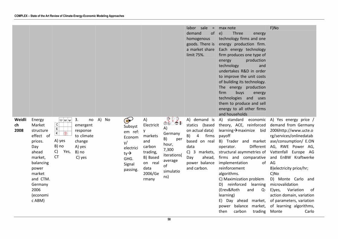
COMPLEX – State of the Art Review of Climate-Energy-Economic Modeling Approaches
58
labor sale = demand of homogenous goods. There is a market share limit 75%.
max note e) Three energy technology firms and one energy production firm. Each energy technology firm produces one type of energy production technology and undertakes R&D in order to improve the unit costs of building its technology. The energy production firm buys energy technologies and uses them to produce and sell energy to all other firms and households
F)No
Weidlich 2008
Energy Market structure effect of prices. Day ahead market, balancing power market and CTM. Germany 2006 (economic ABM)
E
C E €
C
€
A) yes B) no C) Yes, CT
3. no emergent response to climate change A) yes B) no C) yes
A) No Subsyst
em ref: Economy/ electricity GHG. Signal passing.
A) Electricity markets and carbon trading, B) Based on real data 2006/Germany
A) Germany B) per hour, 7,300 iterations(average of simulations)
A) demand is statics (based on actual data) B) 4 firms based on real data C) 3 markets, Day ahead, power balance and carbon.
A) standard economic theory, ACE, reinforced learningmaximize bid payoff B) Trader and market operator. Different structural asymmetries of firms and comparative implementation of reinforcement algorithms. C) Maximization problem D) reinforced learning (Erev&Roth and Q-learning) E) Day ahead market, power balance market, then carbon trading
A) Yes energy price / demand from Germany 2006http://www.ucte.org/services/onlinedatabase/consumption/ E.ON AG, RWE Power AG, Vattenfall Europe AG and EnBW Kraftwerke AG B)electricity price/hr; C)No D) Monte Carlo and microvalidation E)yes, Variation of action domain, variation of parameters, variation of learning algorithms, Monte Carlo

COMPLEX – State of the Art Review of Climate-Energy-Economic Modeling Approaches
59
market. per hour, 7,300 iteration (average of simulations)
distribution for each test. F) yes
Sopha 2013
Adoption of clean heating systems in Norway /policy (Empirical- rules + computational organization ABM)
EC E €
C
€
A) No (evolution of market under 3 value systems) B) NO C) NO
3. no emergent response to climate change A) yes B) no C) yes
A) No subsyst
em reference: One way household decision making, economyGHG
A)Household heating B) No energy types
A) Micro level based on survey in Norway 5/year 2001-2009 B)30 simulations, 3 month step 2000-2020 (20 years)
A) Probabilistic choice based on 3 types of value system + network effects. B) STATIC
A) Not modeled
a) Theory Of Planned Behavior, Diffusion Of Innovation Theory, Meta-Theory Of Planned Behavior, Utility Theory. b) 3 types of household with 4 decision strategies and 5 value systems for probability of adoption. (+ comparison with implementations of small world network, random network and spatial network ) c) behavior satisfaction (3 rule/probabilistic model + network influence) d) Network interaction (spatial, small world and random), strategy selection, selection of energy type, installation of heating system.
A) All parameters are based on survey. B) fractions of adoption / time C) Distributional equivalence with data, but it doesn’t fit fully. D) Yes (but), boundary adequacy, 3rd party programmer validation, sensitivity to @ 0 parameterization E) distributional equivalence with benchmark, goodness of fit F) No UML, but conceptual diagram with parameters
Kempener 2009
Personal carbon trading UK / evolution of CM (Microeco
E
C E €
C
€
No (evolution of
3. no emergent response to climate change A) yes B) no
a)No One
way, economy energy
A) Electricity, carbon trading, B) Stylized
A)UK (ONS 2008 The FES 2005-2006) B)10
A) demand in terms of adoption rates (relaxation of utilitarian rationality) B) static
A)general economic theory B) quintiles based on income profiles C) maximization (only for the firms who have different investment
A) Static decision rules/multi-criterion optimization. B) Carbon Price, Ton Co2, allocations and emissions, fuel poverty, average technology

COMPLEX – State of the Art Review of Climate-Energy-Economic Modeling Approaches
60
nomic + empirical-rules ABM)
market under 3 behavioral rules) B)NO C) Yes, CT
C) yes consumption
based on GHG profile
years C) perfect market/neoclassical theory
criterion, demand is homogenous, goods are homogenous, D) Probabilistic rules E) ~10/year for 10 years
uptake C)No D)No E)No F)No
Nannen, Veb Den Berg 2010
Comparison of tax on fossil fuels, prize policy and advertisement policy in terms of the evolution of energy market shares. (microeconomic ABM)
E
C E €
C
€
A)Climate change (emission/energy type) as part of utility function B) at Int and comparatively but no interaction of MBI during run time.
3. no emergent response to climate change A) yes B) no C) yes
A) (Tech Dev) Only In Terms Of Market Share
One way, PUBLIC POLICYenergy type as constrain in economic maximization
A) electricity B) Stylized Electricity production: Fossil energy and renewable
A)No spatial domain B) 400 time steps, simulating 400 quarters or 100 years
A) demand is exogenous B) Investment and divestment based of C) Not fully modeled
A) Evolutionary economics, network theory, general economic theory (Each agent’s controls internal supply and production, via standard economic growth and production functions. Some allocations receive higher yield and the agent optimizes such strategy. There is mutation and crossover (neighborhood effect). B) maximization problem (heterogeneous strategies determined by welfare maximization and network influence (small world). 400(int)200(end) agents, heterogeneous in terms of the intimal parameters(3d vector in Boolean matrix) C) Random mutation and neighborhood imitation
A) No B) GROWTH EFFECT, INCOME , TEMP (NOT QUANTITATIVE METRICS BUT RATE OF CHANGE?) Income , Growth Rate And Temperature As Functions Of Taxes C) No D) No E) No
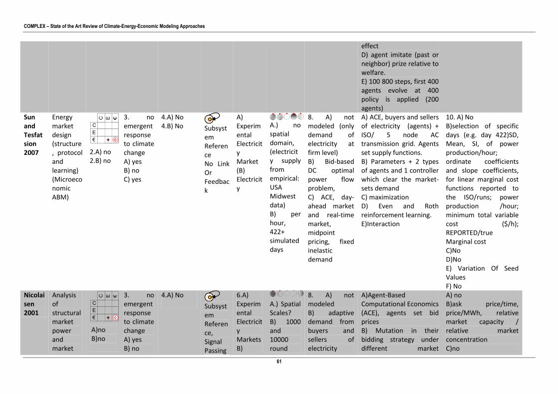
COMPLEX – State of the Art Review of Climate-Energy-Economic Modeling Approaches
61
effect D) agent imitate (past or neighbor) prize relative to welfare. E) 100 800 steps, first 400 agents evolve at 400 policy is applied (200 agents)
Sun and Tesfatsion 2007
Energy market design (structure, protocol and learning) (Microeconomic ABM)
E
C E €
C
€
2.A) no 2.B) no
3. no emergent response to climate change A) yes B) no C) yes
4.A) No 4.B) No Subsyst
em Reference No Link Or Feedback
A) Experimental Electricity Market (B) Electricity
A.) no spatial domain, (electricity supply from empirical: USA Midwest data) B) per hour, 422+ simulated days
8. A) not modeled (only demand of electricity at firm level) B) Bid-based DC optimal power flow problem, C) ACE, day-ahead market and real-time market, midpoint pricing, fixed inelastic demand
A) ACE, buyers and sellers of electricity (agents) + ISO/ 5 node AC transmission grid. Agents set supply functions. B) Parameters + 2 types of agents and 1 controller which clear the market-sets demand C) maximization D) Even and Roth reinforcement learning. E)Interaction
10. A) No B)selection of specific days (e.g. day 422)SD, Mean, SI, of power production/hour; ordinate coefficients and slope coefficients, for linear marginal cost functions reported to the ISO/runs; power production /hour; minimum total variable cost ($/h); REPORTED/true Marginal cost C)No D)No E) Variation Of Seed Values F) No
Nicolaisen 2001
Analysis of structural market power and market
E
C E €
C
€
A)no B)no
3. no emergent response to climate change A) yes B) no
4.A) No Subsyst
em Reference, Signal Passing
6.A) Experimental Electricity Markets B)
A.) Spatial Scales? B) 1000 and 10000 round
8. A) not modeled B) adaptive demand from buyers and sellers of electricity
A)Agent-Based Computational Economics (ACE), agents set bid prices B) Mutation in their bidding strategy under different market
A) no B)ask price/time, price/MWh, relative market capacity / relative market concentration C)no

COMPLEX – State of the Art Review of Climate-Energy-Economic Modeling Approaches
62
power due to agent strategy (learning)(microeconomic ABM)
C) yes Electricity
cases.
C) BILATERAL, DOUBLE DIB/CLEARING HOUSE
concentration and capacities C) maximization (set bidding price, if its cleared reinforced the probability of setting the same price again subject to constraints D) MRE algorithm with Softmax modified Roth-Erev individual reinforcement learning algorithm to determine their price and quantity offers in each auction round. For the 10 000 auction rounds per run case, possible price offers were randomly selected within each feasible price offer range, implying that each trader could in principle sample each price 100 times during the course of each run E)Interaction
D)no E) no, (or if variation and comparison of variation in the environmental variables can be it?) f) no
Chappin 2009
effect of CET on the decisions of power companies in an oligopolis
E
C E €
C
€
A)effect of carbon trading
3. no emergent response to climate change A) yes B) no C) yes
4.A) Depends, See Note:
Link, MbiEnergy Tech, Signal Passing
6.A) Electricity Production B) Nuclear, Natural Gas
7.A.) Netherlands 10.B) 75 years, 1 year step
8.Representation of A) static B) Supply is driven by demand and constraint by evolution of model
9. A) 7 electricity firms, 1 markets for electricity, 1 CO2 emission rights, 1 government, 1 market for fuels and electricity import, 1 aggregate consumer agent and 1 environment agent.
10. A) Data used collected by Chappin 2006 B) market share / 3 electricity producers; emission reductions by energy type/time; market share / time

COMPLEX – State of the Art Review of Climate-Energy-Economic Modeling Approaches
63
tic market.(microeconomic ABM)
on electricity production firms decisions B)CET
(Ccgt), Coal(Cfstp), Wind, Clean Coal, Biomass
C) ACE, Spot market
long term behavior: •investment •divestment •choice of technology short term behavior: •selling of electricity •acquisition of fuel •acquisition of co2 rights E) energy providers in the short-term they adjust their operation, long-term they decide on (dis)investment in power generation facilities and technology selection. B) Short-term they adjust their operation, long-term they decide on (dis)investment in power generation facilities and technology selection. C)Behavior satisfaction/maximization D) At each step: •update exogenous scenario parameters• electricity trading• emission trading •fuel trading •investment and divestment
step; C)no D)Yes but not explicit: reference to SD verification test Qudrat-Ullah (2005) and Barlas (1996) (source empirical structure and parameters, direct extreme conditions, boundary adequacy of structure, dimension analysis, face validation, extreme conditions, qualitative future analysis, comparison with accepted theory and an extensive sensitivity analysis E) Parameter variation and 900 simulations, no cluster analysis or discussion on how scenarios where chosen or averaged. Model was sensitive to fuel prices not management decisions. f) conceptual diagram not UML

COMPLEX – State of the Art Review of Climate-Energy-Economic Modeling Approaches
64
Chappin 2012
Adoption of renewable appliance(light bulbs) (microeconomic, empirical-based rules, computational organization ABM)
E
C E €
C
€
A)yes B)Yes, ban of incandescent bulbs, subsidy of LED and tax on incandescent bulbs
3. no emergent response to climate change A) yes B) no C) yes
A)Tech Adoption Not Development
LINK, MBI Energy Tech, Signal Passing
A)Light Bulbs/ Appliances Not Energy B)Source Is Exogenous To Model
A)survey data in Netherlands/EU policy B)40 years
A)yes B) static from survey data c) simple market: max muticriterion of demand / available supply
A) agents check if they need a lamp, then multi criterion max/ reinforced learning and network influence B)50-250 agents C) Multicriterion maximization problem + behavior satisfaction: Households check whether they need to replace lamps that failed. If so, they use information on the lamps for sale, their criteria, their memory and perceptions to choose the best lamps that can replace the broken lamp D) Development of preferences depends on memory and perceptions, as well as interaction in a social network structure: memetic function pj,memory*=0.5×(pj,memory+pj,experience) for failed lamps, and network min of 15 other agents if > 50% of the friend has a certain type pother*=0.5×(pother+pme) E)
A) secondary sources for the agents, but the lamps where primary in Netherlands B)Market share / scenarios (baseline, ban, subsidy, tax) ;money spent/time; electricity intensity/time; perceptions/utility type; C)no D)no, only variation of weight factor for the purchase decisions per simulation scenario. “fit for purpose” (e.g., Holling, 1978, Barlas and Carpenter, 1990 and Qudrat-Ullah, 2005), direct empirical validation of the model's outcomes is not possible as some policies have not and will not be implemented in reality. A number of verification and validation checks were done as a proxy of such a validation. These included a range of structure–behavior tests that focused on the outcomes of purchase decisions by

COMPLEX – State of the Art Review of Climate-Energy-Economic Modeling Approaches
65
consumer agents. E)Activity UML + conceptual diagrams
Tran 2012
Adoption Of Technology: Gas, Diesel, Full Battery Electric (Bev) , Hybrid Electric Vehicle ( Hev ), Plug-In Hybrid Vehicle (Phv) And H2 Fuel Cell (Fc) (empirical rules ABM)
E
C E €
C
€
A)technology adoption based on environmental criterion B)No C)no
3. no emergent response to climate change A) yes B) no C) yes
A) No Link
ConsumptionTech Diffusion, Signal Passing
A)Transport B)Only In Reference To(E.G. Gas Car)
A) No Focus, Use Of Secondary Sources From DE, UK, USA, Etc. B) 30 Steps
A) Dynamic, Network, Probability Constrained By Preferences B)Exogenous C)Not Modeled
A) combining individual choice behavior and network influence. ( DETAILS ) B)100 agents, heterogeneity simulated by variation of parameters (β|θ)) C)behavior satisfaction D)probabilistic + small world network influence, E) mathematical estimation of individual choice preferences (Pij) for BEVs used to derive index, then applied to ABM framework: Prob(t)=1−(1−[1R∗∑Rr=1Lij(βr)])∗(1−[nk/n])∧(∑wijyi/∑wi)
A) secondary sources, journals and company info: Although we parameterize the model with empirical data where possible, the analysis is mostly based on synthetic output data from the model. B)Cumulative adoption patterns/time; probability of adoption/time ; sensitivity analysis and cluster analysis of P, K and Q. C) agent choice uses Monte Carlo, cluster analysis of adoption curves under different scenarios, validation of inputs, for probabilities and 3 agent types (secondary sources) D) sensibility analysis of constants (P, K, Q) E)No
Wittmann 2006
Energy investment and market
E
C E €
C
€
3. no emergent response to climate
A) No
Tech Investment In
A)Residential Building Owner
A) no spatial domain /
A) bounded rationality (typology of agents with
A) Social Miliues (SINUS-Milieu-Typology ) and rationality types. 4 objective functions
A)Ad-Hoc, social milieu typology taken from private company SINUS-Sociovision

COMPLEX – State of the Art Review of Climate-Energy-Economic Modeling Approaches
66
structure (evolutionary, heuristic, microeconomics ABM)
A)yes, energy tech diffusion with link to CO2 B)No C)No
change a)quantitative: search rules/matrix and only one scenario B)no C)no
Specific Domain, Signal Passing
Investment In Electricity, Hot Water, And Room Heating B) Gas, Micro Cogeneration, Solar- Thermal, Oil, Pellets
building owner investment B)
constraints/rules/preferences) (3 stylized types). B) 1step
(find_all, find_by_aspects, find_common, find_next) and 3 search strategies over 27 options in a decision matrix B) 9 agents; variation in search domain, rules, cost, strategy and budget. C)behavior satisfaction D)Ex goals / search rules /environment E) three different hierarchic timeframes, the operational timeframe, the structural timeframe and the scenario timeframe.
www.sociovision.com , decision matrix based on (see note B)Decisions Outcome And Parameters Table C)Not in paper: “Compared to empirical analysis using regression models, the outcomes of the different actor models seem to be reasonable (Lutzenhiser 1993, Schuler 2000).” D)No E)No F)No
Bunn and Oliveira 2001
Assessment of liberization policy New Electricity Trading Arrangements (NETs) of England and Wales (microeconomic ABM)
E
C E €
C
€
A)no B)no
3. no emergent response to climate change A) yes B) no C) yes
4.A) No Subsyst
em Reference No Link Or Feedback
A) Experimental Electricity Market (B) Electricity
A.) no spatial domain, (electricity supply from empirical: England and Wales) B) per hour, 422+ simulated days
8. A) Active demand B) Bid-based DC optimal power flow problem, C) ACE, bilateral forward market + balancing mechanism + imbalance settlement process
A) ACE, buyers and sellers of electricity (agents) + ISO/ 5 node AC transmission grid. Agents set supply functions. B) Parameters + 2 types of agents and 1 controller which clear the market-sets demand C) maximization D) Even and Roth reinforcement learning. E)Interaction
10. A) no B)selection of specific days (e.g. day 422)SD, Mean, SI, of power production/hour; ordinate coefficients and slope coefficients, for linear marginal cost functions reported to the ISO/runs; power production /hour; minimum total variable cost ($/h); REPORTED/true Marginal cost C)no

COMPLEX – State of the Art Review of Climate-Energy-Economic Modeling Approaches
67
D)no E) variation of seed values F) no
* 36 Bakam 2012
Cost effectiveness analysis with transaction cost of MBI/GHG mitigation in agriculture (individual based model / not ABM)
EC E €
C
€
A)no B)Emission tax, N tax, permit trading
3. no emergent response to climate change A) no B) no C) yes
A)No
MBIFarm Signal Passing
A)Agriculture B)
A)MICRO, farm level B) 40 years, from 100-60% reduction in emission permits
A) Static, from aggregated second source data B)Static, from aggregated second source data C) WTP/WTA + % premium (transaction cost)
The market sets the permit price as the Nash equilibrium value between willingness to pay (WTP) and willingness to accept (WTA), weighted by supplies and demands. The price per unit permit (p) is calculated as: A)
B)no heterogeneity C)Maximization D)static + premium for transaction cost E) S/D, Each Year Emission Permit Is Decreases By 1%. Agent Have To Pick From
A) Aggregation of secondary sources: Scottish executive 2003, IPCC 2006, Radov et al. (2007) and Moran et al. (2008) B)average emission reductions; abatement cost/farm; average abetment cost on farm per unit; cost effectiveness for a tax rate C) NO D) NO E) NO F) NO
Li 2012
investigate the bidding optimization of a wind generation company in the
E
C E €
C
€
A)no B)no
3. no emergent response to climate change A) yes B) no C) yes
4.A)No
5.A)
Electricity GenerationMarket. Signal Passing
6.A) Renewable Energy Production B) Wind
7.A.) Based on the USA WSCC 10.B) 24h / 31 days
A)Static demand B) Supply and demand (static) in energy C) Single sided Auction, Day Ahead / Iso
A)ACE, MATPOWER 4.0 (9-bus 3-Generator Power System) B) Buyers And Sellers Have Different Preferences, Cost And Learning Parameters C) Maximization D) Variant Roth–Erev reinforcement learning
A) Empirical Parameterization? B)forecasting errirs/time;energy gen & sold /time; Average LMPs/time C)Structural Validation? D)no E)no f) No, but circuit
36
* On the margin of being considered an ABM, so it was not used for the summary.

COMPLEX – State of the Art Review of Climate-Energy-Economic Modeling Approaches
68
deregulated day-ahead electricity wholesale market (microeconomic ABM)
(VRE-RL) (Sun 2007) E) Earn Money, Clear Market, Set Bid, Accept Bids, Iso Match Bids,
diagram and conceptual diagram.
Shafiei 2012
Evolution of market shares of electric vehicles (heuristic rules, microecnomic ABM)
E
C E €
C
€
A)renewable transport technology forecasting B)vehicle tax, economic feedbacks (future price of fuel and EV)
3. no emergent response to climate change A) yes B) no C) yes
4.A) No Tech Development But Evolution Of Technology Based On Projected Changes
5.A) SocioeconomicTechnologyEnergy Use, Signal Passing
6.A) Electric Vehicles B) Electricity And Gasoline
7.A.) Iceland car demand 10.B) 2012–2030
8. A) Demand vehicles is discrete (activated and not constant) and then multinomial logit (MNL) B) Supply of EV is based on explicit scenarios C) Simple market, no clearing or auction mechanism
9. A)Consumer choice probability based on the heterogeneous preferences and market share conditions of the EV B)sico-demographic attributes, preferences, and decisions C) Yes, behavior satisfaction and heuristic optimization based on multinomial logit (MNL) D) adaptive expectation formation base don the response and decay of social exposure E)Interaction
10. A) yes, primary for car attributes and Icelandic socio-economic variables and secondary for consumer choice preferences B)Share of EV / time; gasoline consumption /time C) no D)Statistical Test? E)yes, consumer preferences f) yes, action UML

COMPLEX – State of the Art Review of Climate-Energy-Economic Modeling Approaches
69
Deissenberg 2008
Modeling of the EU labor market (NUTS-2) www.eurace.org (Assumption or calibration based ABM)
E
C E €
C
€
A)no B)no
3.no emergent response to climate change A) yes B) no C) yes
4.A) No
5.A) EconomyEconomy, Complex Data Structure (String)
6.A) Labor Market B) None
7.A.) EU 10.B) 4000 days (step)
8. A) demand only in terms of jobs and employees B) Supply of labor and jobs C) No market
A)State-Transition system (x-machine. households (up to 107), firms (up to 105 producing consumption goods, and up to 102 producing investment goods), and banks (102). Other agents, that is, national governments and the single central bank, follow simple, predefined decision rules, B) types of agents and initial conditions (not clear how) C)behavior satisfaction D) the functions are not described. ”reading of messages”(application and job offers) E)event based, message activatedresponse
A) No B)Unemployment rate/time ; % change in wage/time C)no D)no E)no f) yes
Balbi 2012
Assessment of 3 climate and economic adaptation strategies to climate change in alpine
E
C E €
C
€
A)no B)no
3 yes, emergent response to climate change .A) Yes 3.B) No 3.C) Yes
4.A)No 5.A)
Multiple Feedbacks
6.A) EU Tourism And Restaurant In Alpine Region B) Only Energy Consumption,
7.A.) winter tourism socio-ecosystem of Auronzo di Cadore, located in the
8. A) Demand of tourism/services B) energy supply not modeled C) simple, but there is competition between firms
9. A)stakeholder participatory B) socio-economic background and activity targets C)yes, maximization and behavior satisfaction D)Expectation Formation E) Multiple levels of interaction
10.A) Yes, record from 1985-2000 B) Macro Metric Output C) yes, data fitting/calibration with record from 1985-2000 D) Yes E) Yes F) Yes, Static Class UML

COMPLEX – State of the Art Review of Climate-Energy-Economic Modeling Approaches
70
tourism, (participatory, space theory, microeconomic ABM)
Cost / Efficiency
Dolomites (Italy), B) 1day/step, 364 steps
Natarajan 2011
Comparative assessment of DECarb model and historical data agaist DECarb-ABM (assumption or calibration ABM)
E
C E €
C
€
A) B)
3.not explicitly and not in regards to climate change A) yes B) no C) yes
4.A) No
5.A) human building interaction on energy use (energy use/construction)
6.A) construction, activities of households B) electricity
7.A.) UK 10.B) 20 steps, 30 years, 1965-1995
8. A) The demand of energy is modeled but it is not explicit what function or variables are used. B) no supply of energy and not explicit how supply of housing is modeled C) no market
9. A) Theoratical Behavior To Test The Capability Of ABM. Agenst As Marionetes (Gulyas 2005) B)200 Households, One Building Contractor: Household Income; Installation By Neighbors And; Government Policy. C) No D) No E)Interaction
10. A) Comparison With Decarb-EBM Which Was Validated Using Back Casting From 1996-1970 Using Data From Digest Of UK Energy Statistics, DUKES) B) Deviation From Decarb-EBM And DUKES. C) Against Decarb-EBM And DUKES. D) Mean Percentage Deviation / 5 Years E) No F) No
Zhang 2011
Office energy consumption (institution based ABM)
E
C E €
C
€
A)no B)no
3. No non-liner response to climate change A) yes B) no, C) yes
4.A) no
5.A) Sub system signal
6.A) academia (office) B) electricity
7.A.) School of computer science 10.B) 24 days at hr/step
8.Representation of A) Demand B) Supply C) Market
9. A)Based on previous studies on electricity consumption (Firth 2008) and stereotypes based from survey and state machines to represent the computer and light appliances B)3, 4 types of stereotypes C) no
10. A) School wise empirical survey of staff and PhD students B)electricity consumption/time C)no D)no E)n o f) Yes, state chart

COMPLEX – State of the Art Review of Climate-Energy-Economic Modeling Approaches
71
D)no E) activation of lights or computers states.
Matsumoto 2008
GHG ET comparison between ABM and conventional regression model (assumption and/or calibration based ABM)
EC E €
C
€
A)no B)ET
3. No non-liner response to climate change A) yes B) no, C) yes
4.A) no
5.A) subsystem reference (energy market)
6.A) electricity markets B) generic electricity production
7.A.) Chicago Climate Exchange (CCX) 10.B) dec 2003,2004, per week, 52 weeks total. 200 simulations.
8.Representation of A) Demand B) Supply C) Complex system
9. A)ACE tradition B) perception, prediction, strategy, determination, learning parameters. C) yes, 100 agents, 3 strategies/constrains D)yes adaptive: perception, prediction, strategy, determination, learning steps. E)Interaction
10. A) Chicago Climate Exchange (CCX) B)Macro Metric Output C)comparison with linear multiple regression model, D)ME, MAE, RMSE E)no f) no but descriptive diagram.
Jackson 2010
End-use forecast model to evaluate energy efficiency and smartgrid program targets over a fifteen-year horizon. (microeconomic and
E
C E €
C
€
A)Links Between Climate And Energy B)yes, individual utility programs, building efficiency
3. No non-liner response to climate change A) yes B) no, C) yes
4.A) no
5.A) subsystem reference (energy market)
6.A) electricity consumption at the household level B) electricity
7.A.) US Midwest 10.B) 15 years, 2010-2025
8. A) 1000 agents dynamic demand B) change in parameters based on projections C) simple demand drives supply
9. A)Adjustment of End use model: Electricity use is Represented as the product of the number of single family air conditioning customers(CUST),average base year single family/ Central air conditioner kWhuse(UEC) and factors that, overtime, reflect changes in equipment utilization(U), efficiency(E) and dwelling unit thermal efficiency(TE).
10. A) sample of 1350 Duke Indiana residential customers including the electricity use, hourly loads, income, demographics. US Census data for the utility service area(US Census Bureau, 2009). 2001 and 2005 Residential Energy Consumption Databases(US Department of Energy,2009c). B)% Sg end-use potential/annual

COMPLEX – State of the Art Review of Climate-Energy-Economic Modeling Approaches
72
assumption and/or calibration based ABM)
standards, increasing electricity prices,
B) 1000 agents: income, energy demand, efficiency of infrastructure, C) no D) no E) electricity demand driven
income;GWh/year;MW/year C)yes D)no E)no f) no

COMPLEX – State of the Art Review of Climate-Energy-Economic Modeling Approaches
73
5. Overview of Climate-Energy-Economic System Dynamic Modeling
5.1 Introduction
Originally created in 1957 by Jay W. Forrester at MIT, system dynamics is a computer simulation paradigm
aimed at analysis of complex nonlinear dynamic systems and their performance (Forrester, 1971; Sterman,
2000). System dynamics describes various social, economic, technological and environmental systems as
structures consisting of stocks and flows, positive and negative feedbacks, and limiting factors (Radzicki,
2009). While initially system dynamics models were essentially the models of corporations that did not
perform properly, and the ultimate goal of modeling was to design policies to improve their operation,
rather soon the methodology was applied at macro- and global level, particularly to produce projections of
global economic dynamics under natural resource constraints and finite capacity of pollution sinks (the
seminal studies are “World Dynamics” (Forrester, 1971) and “Limits to Growth” (Meadows et al. 1972,
1992, 2002)). System dynamics modeling has particularly long track record in energy economics (see e.g
the recent reviews by Kiani et al. (2010) and Ford (2011)). Applications to economics of climate change
include e.g. the model FREE (Fiddaman, 2002) that is currently being advanced further into the model En-
ROADS (Sterman et al., 2013), and other models some of them are reviewed below.
The mathematical core of any system dynamic model is an (almost always) nonlinear dynamic system
consisting of first-order ordinary differential equations (ODEs). It is well known that only a limited number
of nonlinear ODEs (and even more limited number of systems of nonlinear ODEs) has exact analytical
solutions. Therefore from the very beginning the system dynamics models were implemented through
numeric integration of systems of ODEs. The complexity of system dynamics model varies substantially:
the number of variables may be from the order of tens (as in simplest models) and up to tens of millions (as
e.g. in the ASTRA transport assessment model (Fiorello et al., 2010)).
5.2 Climate-Energy-Economic SD review
5.2.1 Review of general criteria as applied to SD modeling
1) Links between climate, energy and economy
In many system dynamics models the links between climate, energy and economy are realized more or less
along the same lines as in the Integrated Assessment models and CGE models (e.g. through introduction of
emission intensities, climate damage functions etc.). However we provide below some examples of notable
exceptions and ramifications.
Robert U. Ayres, a strong proponent of matching the methodology of energy and resource economics with
basic concepts of thermodynamics, developed the REXS system dynamics model (Resource – EXergy
Service) in which “useful work” enters the production function instead of “raw energy” (a conventional
approach). This led to model better fitting the historical data on growth of the US economy (Ayres and
Warr, 2005).
In an endogenous business cycle climate-economy model NEDyM (Non-Equilibrium Dynamic Model)
(Dumas et al., forthcoming; Hallegatte and Ghil, 2008; Hallegatte et al., 2007; Hallegatte et al., 2008) which
can be regarded as a system dynamics model, the economic impacts of natural disasters (including extreme
weather and climate events) are modeled as instant, discontinuous shocks (instead of using a
climate/environmental damage function of climate/environmental variables smoothly varying in time).
Among important finings obtained with NEDyM are the revealed sensitivity of magnitude of economic
impacts of extremes to their timing relative to the phase of the business cycle (in case of a stand-alone
extreme event) or to their distribution function (in case of a random sequence of extreme events).
In a simulation of possible western US and Canada power industry response to a carbon market (the WSU
model) (Ford, 2008; Ford, 2011) a challenge of representing the power flows across transmission grids and
COMPLEX – State of the Art Review of Climate-Energy-Economic Modeling Approaches
74
electricity prices in each model area – the task for which the traditional system dynamics paradigm of
stocks and flows would not be the best choice as the model developers argue – was overcome by
augmenting the climate-energy-economy system-dynamics model by a supplementary module developed by
other programming tools than the model itself and based on traditional power system methods (a reduced
version of a direct-current optimal power flow calculation ) (Ford, 2011).
2) Potential to represent non-linearities, thresholds and irreversibility
As system dynamic models may be perceived as real-world applications of formal mathematical theory of
nonlinear dynamic systems, it is quite obvious that they are perfectly suited to represent nonlinearities (by
definition) and threshold effects. With respect to applications to economics of climate change, nonlinearities
and thresholds can be observed both in economic modules (e.g. economic crises, bubbles on asset markets
etc.) and climate modules (e.g. abrupt climate change) of coupled climate–socioeconomic system dynamics
models.
As an example of a threshold effect, we would refer to bifurcation of GDP losses caused by extreme
weather and climate events as observed in NEDyM (Hallegatte et al., 2007): GDP losses increase sharply
beyond certain threshold value of the intensity and frequency of extremes.
A question of addressing irreversibilities is slightly more subtle. Formally, dynamic systems are reversible
by definition, as they can be run in inverse time. However the systems converging to attractors are often
practically irreversible as the transient motion cannot be reconstructed with satisfactory accuracy by
starting from the vicinity of the attractor and inverting the time (Lorenz, 1993).
3) Pervasive technological developments
Pervasive technological developments, such as spillovers, can be rather straightforwardly incorporated in
system dynamics models.
4) Positive feedbacks
Positive feedbacks (as well as negative feedbacks) are, by definition, at the very core of system dynamics
modeling paradigm. For a detailed description of positive feedbacks (e.g. related to methane emissions) in a
system dynamics climate model C-ROADS (Climate Rapid Overview And Decision Support) which is
currently being incorporated in a climate-energy-economy model En-ROADS, see Sterman et al. (2013).
5) Representation of economic sectors
Detailed sectoral disaggregation is a rare feature of system dynamics models, with a notable exception of
energy sector (e.g. as in the climate-energy-economy model FREE (Fiddaman, 2002) and in the US energy
supply and demand model FOSSIL2 (Naill, 1992) applied in an early assessment of US national climate
mitigation policies (Naill et al., 1992)). An outstanding example of a very detailed representation of a
particular economic sector in a system dynamics model with environmental applications is the transport
sector in ASTRA model (Fiorello et al., 2010) that was applied to assessment of EU climate mitigation
policies.
6) Energy sources As mentioned before, in many system dynamics models the energy sector is represented in a fairly detailed
manner, therefore many energy sources are considered. E.g. FOSSIL2 (Naill, 1992) includes the following
energy sources: conventional oil (onshore/offshore), enhanced oil, shale oil, conventional gas
(onshore/offshore), unconventional gas, LNG, underground coal, surface coal. The WSU model (Ford,
2008) includes various energy sources for electricity generation: oil, gas, coal, hydropower, nuclear energy,
wind, biomass etc.
7) Mitigation strategies/policies
As all climate-economy models, system dynamics models consider certain mitigation options. The WSU
model (Ford, 2008) has been designed to assess the response of regional electricity sector to introduction of
carbon price (regardless of whether it would have been induced by carbon taxes or tradable permits). The
FREE model (Fiddaman, 2002) distinguishes between carbon taxes and tradable permits and suggests that
taxes would be a more efficient mitigation instrument. Simulations with the FOSSIL2 model (Naill et al.,
1992) acknowledge reforestation as a promising mitigation alternative to carbon taxes or energy efficiency
standards.

COMPLEX – State of the Art Review of Climate-Energy-Economic Modeling Approaches
75
8) Temporal and spatial scales
Usually temporal scales adopted in system dynamics models under review are typical to all climate-energy-
economy models: decades to centuries. Spatial scales differ: while some models are global, as e.g. FREE
(Fiddaman, 2002), others are national or regional, as FOSSIL2 (Naill, 1992), ASTRA (Fiorello et al., 2010),
DEEPS (Assuring…, 2011) and the WSU model (Ford, 2008).
5.2.2 Review of approach-specific criteria as applied to SD modeling
As mentioned before, system dynamics can be regarded as “applied theory of nonlinear dynamic systems”.
Therefore we believe that the two following approach-specific criteria emerging from “basic theory of
nonlinear dynamic systems” can add value to a list of general criteria reviewed in Sec. 5.2.1:
1) Regular vs. chaotic dynamics
While climate dynamics is generally believed to be regular, it has been argued that real-world economic
dynamics might be chaotic (in a sense of deterministic chaos). Lorenz (1993) and Rosser (1997) provide,
among others, reviews of macroeconomic models that are characterized by chaotic dynamics, as well as of
the empirical studies revealing chaotic footprints in real-world economic data series. So is the dynamics of
coupled climate-socioeconomic system regular or chaotic? We are unaware of any applied climate-energy-
economy model that demonstrates chaotic dynamics, however we would like to drive attention of the reader
to a fruitful theoretical work by Chen (1997) demonstrating (within the optimization paradigm, not within
system dynamics approach) that coupled climate-economic model in which both climate and economic
module exert regular dynamics in stand-alone mode, can nevertheless manifest the chaotic behavior when
mutual feedbacks between the two modules are switched on.
2) Continuous vs. discrete time
Although in “basic theory of nonlinear dynamic systems” and its theoretical economic applications both
discrete-time and continuous-time models seem to be equally important (Lorenz, 1992), the applied system
dynamics paradigm normally implies integration of model equations in continuous time. As a notable
exception, we would refer to the E3MG model (Energy–Environment–Economy Model at the Global level)
(Barker, Scrieciu, 2010) which can be regarded as a non-conventional discrete-time system dynamics model
of high complexity.
5.3 Discussion
In an urgent need for innovative approaches to climate-energy-economy modeling (Giupponi et al., 2013)
traditional system-dynamics models, as well as some recent advances to the approach, can certainly play a
role in improving the assessment of climate mitigation policies. Particularly, we believe that the recently
proposed actor-based system dynamics approach (Weber et al., 2005; Hasselmann and Kovalevsky, 2013)
has some added value to traditional system dynamics paradigm. Actor-based system-dynamics approach
borrows from traditional system dynamics its mathematical foundations (treatment of the climate-
socioeconomic system as a complex nonlinear dynamic system with stocks and flows, positive and negative
feedbacks) but interprets the system under study as a system of few powerful aggregated economic actors
interacting and evolving under a conflict of interests. The economic behavior of actors is determined by
actor control strategies responding to the changing state of economic system. Actor-based system-dynamics
approach (also known as multi-actor modeling) has also certain common points with agent-based modeling
(agent-base modeling) reviewed in Chapter 4 the main differences being in a number of actors/agents (few
actors in multi-actor models vs. a multitude of agents in agent-base models) and in their character
(aggregated actors in multi-actor models vs. “true” individual agents in agent-base modeling).

COMPLEX – State of the Art Review of Climate-Energy-Economic Modeling Approaches
76
6. Summary
This report aimed to review the main characteristics of the existing Energy-Climate-Economic models that
are used for the socio-economic and environmental impact assessment of climate and energy related
policies and support decision making in this arena. The focus here was on the modeling approaches that will
be utilized in the COMPLEX WP5 system of economic-energy-environmental models covering both more
traditional modeling techniques such as Computational General Equilibrium (CGE) model and Integrated
Impact Assessment model (IAM) as well as more recent innovative approaches to model complex systems
including agent-based modeling (ABM) and system dynamics (SD) modeling. In addition, it aimed to shed
more light on the mode including the difficulty to represent pervasive technological developments, the
difficulty to represent non-linearities, thresholds and irreversibility, and the insufficiently developed
representation of economic sectors with a significant potential for mitigation and resource efficiency.
In Chapter 2 Climatic IA modeling is reviewed. Climate IA models are fundamental tools when assessing
mitigation strategies, estimating the costs and informing decision makers in order to prevent anthropogenic
climate change. It is even beginning to be used to evaluate the mitigation-adaptation trade-offs. However,
IA models are limited by the weaknesses in their underlying knowledge and by the simplifications required
for efficient modeling and simulation. Many IA models suffer from a lack of transparency in terms of both
policy relevance and credibility. Some other controversial characteristics include: the dominant sequential
approach, the difficulty to represent pervasive technological developments and non-linearities, thresholds
and irreversibilities, the treatment of climate change damages, the omission of other human-disturbances,
the discount rate values, the consideration of equity across time and space, structural shifts in socio-
economic systems, etc. The utility of the climate IAM based on Cost-Benefit Analysis has been greatly
disputed since its start due to the number of “empirically and philosophically controversial hypotheses”, as
discussed in Chapter 2.
As (Tol, 2006; Vuuren et al., 2012, 2011c) argue, one of the main challenges to future IAM developments is
the full-coupling with the Earth System Models (ESM) having difficulties of mapping from natural to
economic space and back (Tol, 2006), and relating mental models of the economic agents with the natural
agents “reactions”.
As discussed in Chapter 2, the choice of the discount rate is an issue inherent to the economics of climate
change and not just to IAM, though the longer time horizons in these models make this issue more
important (cf. (Stern, 2006) Report)
There have been rapid advances in recent years in the area of including endogenous technological change;
the review by (Kahouli-Brahmi, 2008) offers a thorough description of the most recent attempts to model
endogeneity and induced technological innovation.
Climatic IAM must be seen as a science in continuous evolution, in which new dimensions of the problem
have to be incorporated by using new methodologies and scopes, and models have to integrate continuously
new scientific knowledge and deepen and diversify the assessments.
The Environmental CGE models which are frequently used to assess impact of environmental and energy
relate d policies are reviewed in Chapter 3. These models are all (recursive) dynamic and treat international
trade such that goods with the same statistical classification but different countries of origin are treated as
non-perfect substitutes. Single-country models tend to be more detailed in terms of sectors and household
types, and they are in general used for analyses of country-specific policy issues and proposals. Multi-
country and global models, on the other hand, tend to have less sector detail and to be designed for analysis
of proposed multi-lateral policies such as free-trade agreements. In the case of environmental CGE models
the multi-country and global models in most cases are designed for analysis of trans-boundary pollution
problems.
In these environmental CGE models Technological changes are modeled utilizing different approaches. In
some models technology improvements are represented over time (exogenously), and advanced

COMPLEX – State of the Art Review of Climate-Energy-Economic Modeling Approaches
77
technologies are included. Some models formulates production technologies in an endogenous manner
allowing for price-driven derivation of all intermediate consumption and the services from capital and labor.
Most of the models reviewed here make use of abatement cost functions (abatement curves) are used. These
can be seen as ad hoc rules to describe the trajectories of these emissions, following current international
modeling practice. There is no damage function in environmental CGE models, that links emissions growth
to economic output through climate change or otherwise. Even if there is no direct feedback from the
environment module to the economic module, emission restriction policies will have impacts on the
economic module and hence, there is a strong link between the economic module and the environment
module.
Chapter 4 reviews the climate-energy-economy agent-based modeling. The application of ABMs to climate-
economy-energy systems reviewed in this chapter consisted mostly of microeconomic, empirical- or
heuristic rules, evolutionary programming and assumption and/or calibration-based rules. Most cases at
most consist of one link with descriptive reference to another system, e.g. Economy-to-energy: economic
cost of stylized energy types based on their GHG emission profiles. Endogenizing energy economy and
environment feedbacks with robust representations of each respective systems (integrative modeling of
EEC systems) is clearly yet to achieved within ABM, e.g. modeling (micro) economy-to-energy-to-climate-
to-economy. There is also a general ambiguity in terms of justifying the numbers of agents, integration step,
time period, validation technique and treatment of simulation outputs; all these apparent flaws or lack of
methodological rigor are however often justified in terms of the ABM’s purpose, i.e. the quality of a ABM
depends on the application or formulation of the problem. In general terms however it is clear that much of
the promise or potential of ABM’s to address the scientific gaps in energy-economy-climate systems has yet
to be realized.
ABMs treat mitigation strategies in two ways: either by focusing on command and control instruments (e.g.
1987 Montreal Protocol) or focusing on the following market-based instruments (MBI): cap and trade (CT);
public research and development expenditures; and taxes.
There are a few ABMs that explicitly model a non-linear response to climate change. However, All ABM
reviewed have non-linearity and irreversibilities but none had thresholds in the output (clear bifurcations
into stable states). It should also be noted that while ABM is the best method to model non-linearities or
emergent behavior, the fact remains that unless there is a high level multi-threading interface37 or event
based hierarchy in the end, an ABM -as complex as it may be- will effectively run like a linear program,
e.g. System Dynamics or Spatial Econometrics. From the ABM’s reviewed here, we see that the models are
sensitive to prices more than to implementations of bounded rationality or expectation formations.
None of the ABMs reviewed here included endogenous technological development. Meaning that no ABM
reviewed here have modeled an explicit mechanism and/or dynamics for technological innovation.
However, some ABM model investment and divestment into stylized electricity production technologies.
Other ABM’s model transitions in terms of market share of theoretical technologies such as Clean Coal.
Other ABM’s technological end-use and market-share forecasts.
Given the large domain that ABMs cover, it is almost impossible to expect that every parameter and
function in a ABM is derived from empirically validated data; ABM is an exploratory not descriptive
technique. In fact ABM that constrain the functions and parameters of the agents exclusively to empirical
data, often results in very static models (e.g., Sopha 2013). Very few ABMs perform some kind of
Structural validation. When it is performed, it is only for one aspect of the model (e.g. energy generation,
in an energy market). ABMs are in theory capable of having a 1:1 ratio of data granularity, e.g. each survey
or data point, can be represented fully as an aspect on an agent’s heterogeneity. However it is often the case
that ABM’s actually go beyond that and produce experimental data which cannot be validated in any
rigorous way.
37 Multi-threading is a widespread programming and execution model that allows multiple threads (functions) to exist within the context of a single process (time step). These threads share the process' resources, but are able to execute independently.

COMPLEX – State of the Art Review of Climate-Energy-Economic Modeling Approaches
78
Finally, in Chapter 5, the System Dynamics Modeling tool was reviewed and discussed. It was argued that,
traditional system-dynamics models can certainly play a role in improving the assessment of climate
mitigation policies. Particularly, the recently proposed actor-based system dynamics approach (Weber et al.,
2005; Hasselmann and Kovalevsky, 2013) has some added value to traditional system dynamics paradigm.
Actor-based system-dynamics approach borrows from traditional system dynamics its mathematical
foundations, however, interprets the system under study as a system of few powerful aggregated economic
actors interacting and evolving under a conflict of interests. The economic behavior of actors is determined
by actor control strategies responding to the changing state of economic system.

COMPLEX – State of the Art Review of Climate-Energy-Economic Modeling Approaches
79
References
A.B., 2012. Approaching a state shift in Earth/’s biosphere. Nature 486, 52–58.
Ackerman, F., DeCanio, S.J., Howarth, R.B., Sheeran, K., 2009a. Limitations of integrated assessment
models of climate change. Climatic Change 95, 297–315.
Ackerman, F., Stanton, E.A., Hope, C., Alberth, S., 2009b. Did the Stern Review underestimate US and
global climate damages? Energy Policy 37, 2717–2721.
ADB, 2009. The economics of climate change in Southeast Asia: a regional review. Asian Development
Bank, Manila (Philippines).
Akhtar, M.K., Wibe, J., Simonovic, S.P., MacGee, J., 2013. Integrated assessment model of society-
biosphere-climate-economy-energy system. Environmental Modeling & Software 49, 1–21.
Alcamo, J., Shaw, R., Hordijk, L. (Eds.), 1990. The RAINS Model of Acidification: Science and Strategies
in Europe, 1990th ed. Springer.
Annan, J.D., Hargreaves, J.C., 2011. On the generation and interpretation of probabilistic estimates of
climate sensitivity. Climatic Change 104, 423–436.
Anscombe, F. J. (1973). "Graphs in Statistical Analysis". American Statistician 27 (1): 17–21. JSTOR
2682899.
Anthoff, D., Tol, R.S.J., 2012. The climate Framework for Uncertainty, Negotiation and Distribution
(FUND), Technical description, version 3.6.
Arigoni, R., Markandya, A., 2009. Integrated Impact Assessment Models of Climate Change with an
Emphasis on Damage Functions: a Literature Review.
Assuring Ohio’s Competitiveness in a Carbon-Constrained World: A Collaboration between Ohio
University and The Ohio State University, 2011
Axelrod R., R. Conte, R. Hegselmann, P. Terna (Eds.). 1997. Advancing the Art of Simulation in the Social
Sciences in Simulating Social Phenomena, Springer, Berlin (1997), pp. 21–40
Ayres R.U., Warr B., 2005. Accounting for growth: the role of physical work. Structural Change and
Economic Dynamics 16, 181-209.
Azar, C., Lindgren, K., Obersteiner, M., Riahi, K., Vuuren, D.P. van, Elzen, K.M.G.J. den, Möllersten, K.,
Larson, E.D., 2010. The feasibility of low CO2 concentration targets and the role of bio-energy with carbon
capture and storage (BECCS). Climatic Change 100, 195–202.
B. D. McCullough and H. D. Vinod. 1999. The Numerical Reliability of Econometric Software. Journal of
Economic Literature , Vol. 37, No. 2 (Jun., 1999), pp. 633-665 Published by: American Economic
Association
Bakam Innocent, Bedru Babulo Balana, Robin Matthews. 2012. Cost-effectiveness analysis of policy
instruments for greenhouse gas emission mitigation in the agricultural sector. Journal of Environmental
Management, Volume 112, 15 December 2012, Pages 33-44, ISSN 0301-4797,
COMPLEX – State of the Art Review of Climate-Energy-Economic Modeling Approaches
80
Balbi Stefano, Carlo Giupponi, Pascal Perez, Marco Alberti. 2012. A spatial agent-based model for
assessing strategies of adaptation to climate and tourism demand changes in an alpine tourism destination,
Environmental. Modeling & Software, Volume 45, July 2013, Pages 29-51, ISSN 1364-8152
Barker T., Scrieciu S.S., 2010. Modeling low climate stabilization with E3MG: Towards a ‘New
Economics’ approach to simulating energy-environment-economy system dynamics. The Energy Journal
31, 137-164.
Barker, T., Pan, H., Köhler, J.H., Warren, R., Winne, S., 2006. Decarbonizing the global economy with
induced technological changes : scenarios to 2100 using EMG. The energy journal. - Boston, Mass. [u.a.] :
Oelgeschlager, Gunn & Hain, , ZDB-ID 8643192. - 2006, special issue 241–258.
Barker, T., Scrieciu, S., 2010. Modeling Low Climate Stabilization with E3MG: Towards a “New
Economics” Approach to Simulating Energy-Environment-Economy System Dynamics. The Energy
Journal 31.
Barnosky, A.D., Hadly, E.A., Bascompte, J., Berlow, E.L., Brown, J.H., Fortelius, M., Getz, W.M., Harte,
J., Hastings, A., Marquet, P.A., Martinez, N.D., Mooers, A., Roopnarine, P., Vermeij, G., Williams, J.W.,
Gillespie, R., Kitzes, J., Marshall, C., Matzke, N., Mindell, D.P., Revilla, E., Smith,
Bassi, A.M., Shilling, J.D., 2010. Informing the US Energy Policy Debate with Threshold 21.
Technological Forecasting and Social Change 77, 396–410.
Bergman, L. (1990), The Development of Computable General Equilibrium Modeling, in Bergman, L.,
D.W. Jorgenson and E. Zalai (1990), General Equilibrium Modeling and Economic Policy Analysis.
Cambridge and Oxford: Basil Blackwell.
Bergman, L., and Henrekson, M., CGE modeling of environmental policy and resource
management, Handbook of environmental economics 3 (2005): 1273-1306.
Bernard, A., Vielle, M., Viguier, L., 2006. Burden Sharing Within a Multi-Gas Strategy. Energy Journal,
Special Issue 3, 289-304
Böhringer, C., Rutherford, T.F., 2008. Combining bottom-up and top-down. Energy Economics 30, 574–
596.
Bollen, J., Gielen, A., Timmer, H., 1999. Clubs, ceilings and CDM:
Bonabeau, E., Dorigo, M., Theraulaz, G. 2000. Inspiration for optimization from social insect behavior.
Nature. Macmillian Magazines Ltd. 2000/07/06/print 406: 6791: 39-42.1038/35017500. 10.1038/35017500
Borges, A. M., Applied General Equilibrium Models, OECD Economic Studies 7 (1986): 7-43.
Bosetti, V., Carraro, C., Galeotti, M., Massetti, E., Tavoni, M., 2006. WITCH - A World Induced Technical
Change Hybrid Model (SSRN Scholarly Paper No. ID 948382). Social Science Research Network,
Rochester, NY.
Bouwman, A.., Kram, T., Goldewijk, K.K., 2006. Integrated modeling of global environmental change: an
overview of IMAGE 2.4. Netherlands Environmental Assessment Agency, Bilthoven.
Burniaux, J.-M., Truong, T.P., 2002. GTAP-E: an energy-environmental version of the GTAP model.
GTAP Technical Papers 18.
Calvin, K., Edmonds, J., Bond-Lamberty, B., Clarke, L., Kim, S.H., Kyle, P., Smith, S.J., Thomson, A.,
Wise, M., 2009. 2.6: Limiting climate change to 450 ppm CO2 equivalent in the 21st century. Energy
Economics 31, Supplement 2, S107–S120.
Calvin, K., Wise, M., Clarke, L., Edmonds, J., Kyle, P., Luckow, P., Thomson, A., 2013. Implications of
simultaneously mitigating and adapting to climate change: initial experiments using GCAM. Climatic
Change 117, 545–560.

COMPLEX – State of the Art Review of Climate-Energy-Economic Modeling Approaches
81
Capros, P., Georgakopoulos, T., Filippoupolitis, A., Kotsomiti, S., Atsaves, G., Proost, S., van Regemorter,
D., Conrad, K., Schmidt, T.F.N., 1998. The GEM-E3 Model Reference Manual. National Technical
University, Athens
Capros, P., Kouvaritakis, N., Karkatsoulis, P., Fragkiadakis, K., Van Regemorter, D., Zaporozhets, V.,
Capros, P., Proost, S., van Regemorter, D., Conrad, K., Schmidt, T., 1998. The GEM-E3 Model: Reference
Manual, European Commission, Programme JOULE. DG-XII.
Chappin E.J.L., G.P.J. Dijkema. 2009. On the impact of CO2 emission-trading on power generation
emissions, Technological Forecasting and Social Change, Volume 76, Issue 3, March 2009, Pages 358-370,
ISSN 0040-1625, http://dx.doi.org/10.1016/j.techfore.2008.08.004.
Chen Z., 1997. Can economic activities lead to climate chaos? An economic analysis of global warming.
The Canadian Journal of Economics 30, 349-366.
Clarke, L., Edmonds, J., Jacoby, H., Pitcher, H., Reilly, J., Richels, R., 2007. Scenarios of Greenhouse
Gas Emissions and Atmospheric Concentrations. US Department of Energy Publications.
Clarke, L., Edmonds, J., Krey, V., Richels, R., Rose, S., Tavoni, M., 2009. International climate policy
architectures: Overview of the EMF 22 International Scenarios. Energy Economics 31, Supplement 2, S64–
S81.
Contributions to Management Science. ISBN 978-3-7908-2067-6, Physica Verlag Heidelberg (Book)
Cumming, G.S., Alcamo, J., Sala, O., Swart, R., Bennett, E.M., Zurek, M., 2005. Are Existing Global
Scenarios Consistent with Ecological Feedbacks? Ecosystems 8, 143–152.
Davies, E.G.R., Simonovic, S.P., 2010. ANEMI: a new model for integrated assessment of global change.
Interdisciplinary Environmental Review 11, 127–161.
Deissenberg Christophe, Sander van der Hoog, Herbert Dawid. 2008. EURACE: A massively parallel
agent-based model of the European economy. Applied Mathematics and Computation, Volume 204, Issue
2, 15 October 2008, Pages 541-552, ISSN 0096-3003,
Dietz, S., Hope, C., Patmore, N., 2007. Some economics of “dangerous” climate change: Reflections on the
Stern Review. Global Environmental Change 17, 311–325.
Döll, S., 2009. Climate change impacts in computable general equilibrium models: An overview, HWWI
Research Paper, No. 1-26
Dowlatabadi, H., 1998. Sensitivity of climate change mitigation estimates to assumptions about technical
change. Energy Economics 20, 473–493.
Dowlatabadi, H., Morgan, M.G., 1993. A model framework for integrated studies of the climate problem.
Energy Policy 21, 209–221.
Dumas P., Ghil M., Groth A., Hallegatte S., forthcoming. Dynamic coupling of the climate and
macroeconomic systems. Mathematical Social Sciences.
EC, 1996. POLES 2.2. European commission DG XII, EUR 17358.
Edenhofer, O., Knopf, B., Barker, T., Baumstark, L., Bellevrat, E., Chateau, B., Criqui, P., Isaac, M.,
Kitous, A., Kypreos, S., Leimbach, M., Lessmann, K., Magne, B., Scrieciu, S., Turton, H., Vuuren, D.P.
van, 2010. The Economics of Low Stabilization: Model Comparison of Mitigation Strategies and Costs.
The Energy Journal 31.

COMPLEX – State of the Art Review of Climate-Energy-Economic Modeling Approaches
82
Edenhofer, O., Lessmann, K., Bauer, N., 2005. Mitigation Strategies and Costs of Climate Protection: The
Effects of ETC in the Hybrid Model MIND (SSRN Scholarly Paper No. ID 871447). Social Science
Research Network, Rochester, NY.
Edenhofer, O., Lessmann, K., Kemfert, C., Grubb, M., Köhler, J., 2006. Induced technological change:
Exploring its implications for the economics of atmospheric stabilization: Synthesis report from the
innovation modeling comparison project. The Energy Journal 27, 57–107.
Edmonds, J., Luckow, P., Calvin, K., Wise, M., Dooley, J., Kyle, P., Kim, S.H., Patel, P., Clarke, L., 2013.
Can radiative forcing be limited to 2.6 Wm−2 without negative emissions from bioenergy AND CO2
capture and storage? Climatic Change 118, 29–43.
Edmonds, J., Pitcher, H., Sands, R., 2004. Second Generation Model: an Overview.
Edmonds, J., Reilly, J., 1985. Global Energy-Assessing the Future. Oxford University Press, New York.
Edmonds, J., Wise, M., Pitcher, H., Richels, R., Wigley, T., Maccracken, C., 1997. An integrated
assessment of climate change and the accelerated introduction of advanced energy technologies. Mitig
Adapt Strat Glob Change 1, 311–339.
Edmonds, J.A., Pitcher, H.M., Barns, D., Baron, R., Wise, M.A., 1995. Modeling future greenhouse gas
emissions: the second generation model description. Modeling Global Change 295–340.
Emile J.L. Chappin, Maarten R. Afman. 2012. An agent-based model of transitions in consumer lighting:
Policy impacts from the E.U. phase-out of incandescents, Environmental Innovation and Societal
Transitions, Volume 7, June 2013, Pages 16-36, ISSN 2210-4224,
Epstein J.M., R. Axtell. 1996. Growing artificial societies: social science from the bottom up. Washington,
D.C., Brookings Institution Press; MIT Press, (1996).
Fiddaman T.S., 2002. Exploring policy options with a behavioral climate–economy model. System
Dynamics Review 18, 243-267.
Fiddaman, T.S., 2002. Exploring policy options with a behavioral climate–economy model. System
Dynamics Review 18, 243–267.
Fiorello D., Fermi F., Bielanska D., 2010. The ASTRA model for strategic assessment of transport policies.
System Dynamics Review 26, 283-290.
Fischer, G., Tubiello, F.N., van Velthuizen, H., Wiberg, D.A., 2007. Climate change impacts on irrigation
water requirements: Effects of mitigation, 1990–2080. Technological Forecasting and Social Change 74,
1083–1107.
Fisher-Vanden, K., Schu, K., Sue Wing, I., Calvin, K., 2012. Decomposing the impact of alternative
technology sets on future carbon emissions growth. Energy Economics 34, Supplement 3, S359–S365.
Ford A., 2008. Simulation scenarios for rapid reduction in carbon dioxide emissions in the western
electricity system. Energy Policy 36, 443–455.
Ford A., 2011. System dynamics models of environment, energy and climate change. In: Extreme
Environmental Events. Complexity in Forecasting and Early Warning. Meyers R.A. (Ed.). Springer, New
York, pp. 908-927.
Forrester, J., 1971. World Dynamics. Pegasus Communications, Inc., Waltham, Massachussetts.
Forrester, J.W., 1969. Urban dynamics.

COMPLEX – State of the Art Review of Climate-Energy-Economic Modeling Approaches
83
Frank, D.C., Esper, J., Raible, C.C., Büntgen, U., Trouet, V., Stocker, B., Joos, F., 2010. Ensemble
reconstruction constraints on the global carbon cycle sensitivity to climate. Nature 463, 527–530.
Gerst, M.D., P. Wang, A. Roventini, G. Fagiolo, G. Dosi, R.B. Howarth, M.E. Borsuk. 2013. Agent-based
modeling of climate policy: An introduction to the ENGAGE multi-level model framework. Environmental
Modeling & Software, Volume 44, June 2013, Pages 62-75, ISSN 1364-8152,
Gharbi, Q., Le Mouel, P., Delkis, K., 2010. MODELS: MOdel Development for the Evaluation of Lisbon
Strategies. Description of GEM-E2 model improvements.
Giupponi C., Borsuk M.E., de Vries B.J.M., Hasselmann K., 2013. Innovative approaches to integrated
global change modeling. Environmental Modeling & Software 44, 1-9.
Goulder, L.H., Schneider, S.H., 1999. Induced technological change and the attractiveness of CO2
abatement policies. Resource and Energy Economics 21, 211–253.
Gregory, K., Rogner, H.-H., 1998. Energy Resources and Conversion Technologies for the 21st Century.
Mitigation and Adaptation Strategies for Global Change 3, 171–230.
Grimm Volker, Uta Berger, Donald L. DeAngelis, J. Gary Polhill, Jarl Giske, Steven F. Railsback, The
ODD protocol: A review and first update, Ecological Modeling, Volume 221, Issue 23, 24 November 2010,
Pages 2760-2768, ISSN 0304-3800
Grübler, A., Messner, S., 1998. Technological change and the timing of mitigation measures. Energy
Economics 20, 495–512.
Hallegatte S., Ghil M., 2008. Natural disasters impacting a macroeconomic model with endogenous
dynamics. Ecological Economics 68, 582-592.
Hallegatte S., Ghil M., Dumas P., Hourcade J.-C., 2008. Business cycles, bifurcations and chaos in a neo-
classical model with investment dynamics. Journal of Economic Behavior & Organization 67, 57–77.
Hallegatte S., Hourcade J.-C., Dumas P., 2007. Why economic dynamics matter in assessing climate change
damages: Illustration on extreme events. Ecological Economics 62, 330-340.
Hansen, J., Sato, M., Kharecha, P., Beerling, D., Berner, R., Masson-Delmotte, V., Pagani, M., Raymo, M.,
Royer, D.L., Zachos, J.C., 2008. Target Atmospheric CO2: Where Should Humanity Aim? The Open
Atmospheric Science Journal 2, 217–231.
Hansen, J., Sato, M., Ruedy, R., Kharecha, P., Lacis, A., Miller, R., Nazarenko, L., Lo, K., Schmidt, G.A.,
Russell, G., Aleinov, I., Bauer, S., Baum, E., Cairns, B., Canuto, V., Chandler, M., Cheng, Y., Cohen, A.,
Del Genio, A., Faluvegi, G., Fleming, E., Friend, A., Hall, T., Jackman, C., Jonas, J., Kelley, M., Kiang,
N.Y., Koch, D., Labow, G., Lerner, J., Menon, S., Novakov, T., Oinas, V., Perlwitz, Ja., Perlwitz, Ju., Rind,
D., Romanou, A., Schmunk, R., Shindell, D., Stone, P., Sun, S., Streets, D., Tausnev, N., Thresher, D.,
Unger, N., Yao, M., Zhang, S., 2007. Dangerous human-made interference with climate: a GISS modelE
study. Atmos. Chem. Phys. 7, 2287–2312.
Hansen, J., Sato, M., Ruedy, R., Lo, K., Lea, D.W., Medina-Elizade, M., 2006. Global temperature change.
PNAS 103, 14288–14293.
Hanson, D., Laitner, J.A., 2004. An integrated analysis of policies that increase investments in advanced
energyefficient/low-carbon technologies. Energy Economics 26, 739–755.
Hasselmann K., Kovalevsky D.V., 2013. Simulating animal spirits in actor-based environmental models.
Environmental Modeling & Software 44, 10-24.
Held, H., Kriegler, E., Lessmann, K., Edenhofer, O., 2009. Efficient climate policies under technology and
climate uncertainty. Energy Economics 31, Supplement 1, S50–S61.

COMPLEX – State of the Art Review of Climate-Energy-Economic Modeling Approaches
84
Herbert , Simon. 1957. "A Behavioral Model of Rational Choice", in Models of Man, Social and Rational:
Mathematical Essays on Rational Human Behavior in a Social Setting. New York: Wiley.
Hibbard, K., Janetos, A., van Vuuren, D.P., Pongratz, J., Rose, S.K., Betts, R., Herold, M., Feddema, J.J.,
2010. Research priorities in land use and land-cover change for the Earth system and integrated assessment
modeling. International Journal of Climatology 30, 2118–2128.
Hinchy, M., Hanslow, K., 1996. The MEGABARE model: interim documentation. ABARE.
Höök, M., Tang, X., 2013. Depletion of fossil fuels and anthropogenic climate change—A review. Energy
Policy 52, 797–809.
Hope, C., 2011. The Social Cost of Co2 from the Page09 Model (SSRN Scholarly Paper No. ID 1973863).
Social Science Research Network, Rochester, NY.
Hope, C., Anderson, J., Wenman, P., 1993. Policy analysis of the greenhouse effect: An application of the
PAGE model. Energy Policy 21, 327–338.
Hourcade, J.C., Jaccard, M., Bataille, C., Ghersi, F., 2006. Hybrid Modeling: New Answers to Old
Challenges. The Energy Journal 2, 1–12.
Hulme, M., Raper, S.C., 1995. An integrated framework to address climate change (ESCAPE) and further
developments of the global and regional climate modules (MAGICC). Energy Policy 23, 347–355.
IIASA, 1981. Energy in a finite world: report. Ballinger Pub. Co, Cambridge, Mass.
in the day-ahead wholesale electricity markets of single-sided auctions. Applied Energy 99 (2012) 13–22
IPCC SRES, 2000. Special Report on Emissions Scenarios.
IPCC, 1990. IPCC First Assessment Report.
IPCC, 1995. IPCC Second Assessment Climate Change 1995.
IPCC, 2001a. Climate Change 2001: Synthesis Report. A Contribution of Working Groups I, II, and III to
the Third Assessment Report of theIntegovernmental Panel on Climate Change.
IPCC, 2001b. Climate Change 2001. Working Group III: Mitigation.
IPCC, 2007a. Climate Change 2007: Synthesis Report. Cambridge University Press, Cambridge.
IPCC, 2007b. Mitigation of Climate Change - Contribution of Working Group III. Cambridge University
Press.
IPCC, 2011. Special Report on Renewable Energy Sources and Climate Change Mitigation. Cambridge
University Press, United Kingdom and New York, NY, USA.
Jacoby, H. D., Reilly, J. M. , McFarland, J. R., and Paltsev, S., 2005. Technology and Technical Change in
the MIT EPPA Model . MIT Joint Program on the Science and Policy of Global Change. . Report, vol. 125.
Massachusetts Institute of Technology, Cambridge, MA
JCR EC, 2010. Prospective Outlook on Long-term Energy Systems. POLES Manual version 6.1.
Jensen, J., Thelle, M.H., 2001. What are the Gains from Multi-Gas Strategy? Fondazione Eni Enrico Mattei
(FEEM), Nota di Lavoro 23.2002, Milano
Jerry Jackson, Improving energy efficiency and smart grid program analysis with agent-based end-use
forecasting models, Energy Policy, Volume 38, Issue 7, July 2010, Pages 3771-3780, ISSN 0301-4215

COMPLEX – State of the Art Review of Climate-Energy-Economic Modeling Approaches
85
Jones, A.D., Chini, L.P., Collins, W., Janetos, A.C., Mao, J., Shi, X., Thomson, A.M., Torn, M.S., 2011.
Regional-Scale Forcing and Feedbacks from Alternative Scenarios of Global-Scale Land Use Change. AGU
Fall Meeting Abstracts 22, 06.
Kahouli-Brahmi, S., 2008. Technological learning in energy–environment–economy modeling: A survey.
Energy Policy 36, 138–162.
Kainuma, M., 2003. Climate policy assessment: Asia-Pacific integrated modeling [...] [...]. Springer, Tokyo
[u.a.
Kelly, D.L., Kolstad, C.D., 1998. Integrated Assessment Models for Climate Change Control.
Kemfert, C., 2002. An Integrated Assessment Model of Economy-Energy-Climate - The Model Wiagem.
Integrated Assessment 3, 281–298.
Kemfert, C., 2005. Induced technological change in a multi-regional, multi-sectoral, integrated assessment
model (WIAGEM): Impact assessment of climate policy strategies. Ecological Economics 54, 293–305.
Kempener, Ruud. 2009. Simulating Personal Carbon Trading; An Agent-Based Model. SPRU Electronic
Working Paper Series. Environment & Energy Programme, SPRU, University of Sussex. May 2009.
Kiani B., Mirzamohammadi S., Hosseini S.H., 2010. A survey on the role of system dynamics methodology
on fossil fuel resources analysis. International Business Research 3, 84-93.
Kiem, A.S., Verdon-Kidd, D.C., 2011. Steps toward “useful” hydroclimatic scenarios for water resource
management in the Murray-Darling Basin. Water Resources Research 47, n/a–n/a.
Klepper, G., Peterson, S., Springer, K., 2003. DART 97. Kiel Working Papers, vol. 1149. Kiel Institute of
World Economics (IfW), Kiel.
Knorr, W., 2009. Is the airborne fraction of anthropogenic CO2 emissions increasing? Geophysical
Research Letters 36, n/a–n/a.
Knutti, R., 2010. The end of model democracy? Climatic Change 102, 395–404.
Kriegler, E., O’Neill, B.C., Hallegatte, S., Kram, T., Lempert, R.J., Moss, R.H., Wilbanks, T., 2012. The
need for and use of socio-economic scenarios for climate change analysis: A new approach based on shared
socio-economic pathways. Global Environmental Change 22, 807–822.
L., Bertram, C., others, 2013. Description of the REMIND model (Version 1.5).
Latif, M., 2011. Uncertainty in climate change projections. Journal of Geochemical Exploration 110, 1–7.
Leimbach, M., Bauer, N., Baumstark, L., Edenhofer, O., 2010. Mitigation costs in a globalized world:
climate policy analysis with REMIND-R. Environmental modeling & assessment 15, 155–173.
Lenton, T.M., Held, H., Kriegler, E., Hall, J.W., Lucht, W., Rahmstorf, S., Schellnhuber, H.J., 2008.
Tipping elements in the Earth’s climate system. PNAS 105, 1786–1793.
Li Gong, Jing Shi. 2013. Agent-based modeling for trading wind power with uncertainty
Lomborg, B., 2010. Global crises, global solutions. Cambridge University Press, Cambridge.
Lorenz H.-W., 1993. Nonlinear Dynamical Economics and Chaotic Motion. Springer-Verlag, Berlin.
Loulou, R., Goldstein, G., Noble, K., others, 2004. Documentation for the MARKAL Family of Models.
IEA Energy Technology Systems Analysis Programme. Paris.

COMPLEX – State of the Art Review of Climate-Energy-Economic Modeling Approaches
86
Luderer, G., Bosetti, V., Steckel, J., Waisman, H., 2009. The Economics of Decarbonization – Results from
the RECIPE model intercomparison, RECIPE Background Paper, available online at http://www.pik-
potsdam.de/recip.
Luderer, G., Leimbach, M., Bauer, N., Kriegler, E., Aboumahboub, T., Arroyo Curras, T., Baumstark,
Luderer, G., Pietzcker, R.C., Kriegler, E., Haller, M., Bauer, N., 2012. Asia’s role in mitigating climate
change: A technology and sector specific analysis with ReMIND-R. Energy Economics 34, Supplement 3,
S378–S390.
macroeconomics of compliance with the Kyoto Protocol. Energy Journal, Special Issue: The Costs of the
Kyoto Protocol: A Multi-Model Evaluation, pp. 177–206.
Mahecha, M.D., Reichstein, M., Carvalhais, N., Lasslop, G., Lange, H., Seneviratne, S.I., Vargas, R.,
Ammann, C., Arain, M.A., Cescatti, A., Janssens, I.A., Migliavacca, M., Montagnani, L., Richardson, A.D.,
2010. Global Convergence in the Temperature Sensitivity of Respiration at Ecosystem Level. Science 329,
838–840.
Manne, A., Mendelsohn, R., Richels, R., 1995. MERGE: A model for evaluating regional and global effects
of GHG reduction policies. Energy Policy 23, 17–34.
Manne, A.S., Richels, R.G., 2004. MERGE: an integrated assessment model for global climate change, in:
Energy and Environment. pp. 175–189.
Manne, A.S., Wene, C.O., 1992. MARKAL-MACRO: A linked model for energy-economy analysis.
Mastrandrea, M.D., Schneider, S.H., 2001. Integrated assessment of abrupt climatic changes. Climate
Policy 1, 433–449.
Mastrandrea, M.D., Schneider, S.H., 2004. Probabilistic Integrated Assessment of “Dangerous” Climate
Change. Science 304, 571–575.
Masui, T., Hanaoka, T., Hikita, S., Kainuma, M., 2006. Assessment of CO2 reductions and economic
impacts considering energy-saving investments. The Energy Journal 175–190.
Masui, T., Matsumoto, K., Hijioka, Y., Kinoshita, T., Nozawa, T., Ishiwatari, S., Kato, E., Shukla, P.R.,
Yamagata, Y., Kainuma, M., 2011. An emission pathway for stabilization at 6 Wm−2 radiative forcing.
Climatic Change 109, 59–76.
Matsumoto Ken’ichi. 2008. Evaluation of an artificial market approach for GHG emissions trading analysis,
Simulation Modeling Practice and Theory, Volume 16, Issue 9, October 2008, Pages 1312-1322, ISSN
1569-190X
Matsuoka, Y., 1992. Projections of global climate change under carbon taxation using a comprehensive
global environmental model. Global Warming and Economic Growth CGER-1001-92, Center for Global
Environmental Research, Tsukuba, Japan.
McDougall, R., Golub, A., 2007. GTAP-E: A Revised Energy Environmental Version of the GTAP Model.
MEA, 2005. Millennium Ecosystem Assessment. Ecosystems and Human Well-being: Scenarios, Global
Assessment Reports. Island Press.
Meadows D., Meadows D., Randers J., 1992. Beyond the Limits: Confronting Global Collapse, Envisioning
a Sustainable Future. Chelsea Green Publishing, White River Junction, VT.
Meadows D., Meadows D., Randers J., 2002. Limits to Growth: The 30-Year Update. Chelsea Green
Publishing, White River Junction, VT

COMPLEX – State of the Art Review of Climate-Energy-Economic Modeling Approaches
87
Meadows D., Meadows D., Randers J., Behrens W. III, 1972. The Limits to Growth: A Report for the Club
of Rome’s Project on the Predicament of Mankind. Universe Books, New York.
Meadows, D.H., Meadows, D.L., Randers, J., Behrens III, W.W., 1972. The Limits to Growth. Universe
Books.
Meadows, D.H., Randers, J., Meadows, D.L., 2004. The limits to growth: the 30-year update. Chelsea
Green Publishing Company, White River Junction, Vt.
Mesarović, M.D., Pestel, E., 1974. Mankind at the turning point: the second report to the Club of Rome.
Dutton.
Messner, S., 1997. Endogenized technological learning in an energy systems model. J Evol Econ 7, 291–
313.
Messner, S., Strubegger, M., 1995. User’s Guide for MESSAGE III. Rep. WP-95-69, International Institute
for Applied Systems Analysis, Laxenburg, Austria.
Model, in: Kainuma, M., Matsuoka, Y., Morita, T. (Eds.), Climate Policy Assessment. Springer Japan, pp.
17–36.
Morgan, M.G., Dowlatabadi, H., 1996. Learning from integrated assessment of climate change. Climatic
Change 34, 337–368.
Morita, T., Jiang, K., Masui, T., Matsuoka, Y., Rana, A., 2003. Long-term Scenarios based on AIM
Morita, T., Matsuoka, Y., Kainuma, M., Harasawa, H., Kai, K., 1994. AIM-Asian Pacific integrated model
for evaluating policy options to reduce GHG emissions and global warming impacts. Global Warming
Issues in Asia 254–273.
Moss, R.H., Edmonds, J.A., Hibbard, K.A., Manning, M.R., Rose, S.K., Vuuren, D.P. van, Carter, T.R.,
Emori, S., Kainuma, M., Kram, T., Meehl, G.A., Mitchell, J.F.B., Nakicenovic, N., Riahi, K., Smith, S.J.,
Stouffer, R.J., Thomson, A.M., Weyant, J.P., Wilbanks, T.J., 2010. The next generation of scenarios for
climate change research and assessment. Nature 463, 747–756.
Müller Birgit, Friedrich Bohn, Gunnar Dreßler, Jürgen Groeneveld, Christian Klassert, Romina Martin,
Maja Schlüter, Jule Schulze, Hanna Weise, Nina Schwarz, Describing human decisions in agent-based
models – ODD + D, an extension of the ODD protocol, Environmental Modeling & Software, Volume 48,
October 2013, Pages 37-48, ISSN 1364-8152
Naill R.F. A system dynamics model for national energy policy planning. System Dynamics Review 8, 1-
19.
Naill R.F., Belanger S., Klinger A., Petersen E., 1992. An analysis of the cost effectiveness of U.S. energy
policies to mitigate global warming. System Dynamics Review 8, 111-128.
Nakicenovic, N., Riahi, K., 2001. An assessment of technological change across selected energy scenarios.
International Institute for Applied Systems Analysis, Laxenburg.
Nakicenovic, N., Riahi, K., 2003. Model runs with MESSAGE in the context of the further development of
the Kyoto-Protocol, WBGU—German Advisory Council on Global Change. WBGU website.
Natarajan Sukumar, Julian Padget, Liam Elliott. 2011. Modeling UK domestic energy and carbon
emissions: an agent-based approach. Energy and Buildings, Volume 43, Issue 10, October 2011, Pages
2602-2612, ISSN 0378-7788
Negishi, T., 1972. General equilibrium theory and international trade. North-Holland Amsterdam.

COMPLEX – State of the Art Review of Climate-Energy-Economic Modeling Approaches
88
Nicolaisen, J.; Petrov, V.; Tesfatsion, L.. 2001. Market power and efficiency in a computational electricity
market with discriminatory double-auction pricin. Evolutionary Computation, IEEE Transactions on , vol.5,
no.5, pp.504,523, Oct 2001. doi: 10.1109/4235.956714
Nigel Gilbert, Klaus Troitzsch. 2005. Simulation for the Social Scientist. Open University Press. Pub Date:
FEB-05. Pages: 312 ISBN: 9780335216000
Nordhaus, W.D., 1979. The efficient use of energy resources, Monograph (Yale University. Cowles
Foundation for Research in Economics) ; 26. Yale University Press, New Haven :
Nordhaus, W.D., 1992. The “DICE” Model: Background and Structure of a Dynamic Integrated Climate-
Economy Model of the Economics of Global Warming (Cowles Foundation Discussion Paper No. 1009).
Cowles Foundation for Research in Economics, Yale University.
Nordhaus, W.D., 1993. Optimal Greenhouse-Gas Reductions and Tax Policy in the “DICE” Model. The
American Economic Review 83, 313–317.
Nordhaus, W.D., 1994. Expert opinion on climatic-change. American Scientist 82 1, 45–51.
Nordhaus, W.D., 2007. A Review of the“ Stern Review on the Economics of Climate Change”. Journal of
Economic Literature 686–702.
Nordhaus, W.D., 2008. A question of balance: weighing the options on global warming policies. Yale
University Press, New Haven.
Nordhaus, W.D., 2010. Economic aspects of global warming in a post-Copenhagen environment. PNAS
107, 11721–11726.
Nordhaus, W.D., Boyer, J., 2000. Warming the world: economic models of global warming. MIT Press,
Cambridge, Mass.
Paltsev, S., Reilly, J.M., Jacoby, H.D., Eckaus, R.S., McFarland, J.R., Sarofim, M.C., Asadoorian, M.O.,
Babiker, M.H.M., 2005. The MIT Emissions Prediction and Policy Analysis (EPPA) Model: Version 4
(Technical Report). MIT Joint Program on the Science and Policy of Global Change.
Pant, H., 2007. GTEM: global trade and environment model. ABARE Technical Report. www.
abareconomics. com/interactive/GTEM/, accessed 4 October.
PBL, 2008. Towards a Global Integrated Sustainability Model. GISMO 1.0 status report. ( No. PBL Report
550025002). Netherlands Environmental Assessment Agenc, Netherlands.
Popp, D., 2006. Comparison of Climate Policies in the ENTICE-BR Model. The Energy Journal
Endogenous Technological Change, 163–174.
Radzicki M.J., 2009. System dynamics and its contribution to economics and economic modeling. In:
Encyclopedia of Complexity and Systems Science. Meyers R.A. (Ed.). Springer, New York, pp. 8990-9000.
Rao, S., Keppo, I., Riahi, K., 2006. Importance of technological change and spillovers in long-term climate
policy. The Energy Journal 27, 123–139.
Rao, S., Riahi, K., Stehfest, E., van Vuuren, D., Cheolhung, C., den Elzen, M., Isaac, M., van Vliet, J.,
2008. IMAGE and MESSAGE scenarios limiting GHG concentration to low levels. IIASA, Laxenbourg.
Riahi, K., Grübler, A., Nakicenovic, N., 2007. Scenarios of long-term socio-economic and environmental
development under climate stabilization. Technological Forecasting and Social Change 74, 887–935.
Riahi, K., Rao, S., Krey, V., Cho, C., Chirkov, V., Fischer, G., Kindermann, G., Nakicenovic, N., Rafaj, P.,
2011. RCP 8.5—A scenario of comparatively high greenhouse gas emissions. Climatic Change 109, 33–57.

COMPLEX – State of the Art Review of Climate-Energy-Economic Modeling Approaches
89
Rial, J.A., Sr, R.A.P., Beniston, M., Claussen, M., Canadell, J., Cox, P., Held, H., Noblet-Ducoudré, N. de,
Prinn, R., Reynolds, J.F., Salas, J.D., 2004. Nonlinearities, Feedbacks and Critical Thresholds within the
Earth’s Climate System. Climatic Change 65, 11–38.
Richmond, B., 1993. Systems thinking: Critical thinking skills for the 1990s and beyond. System Dynamics
Review 9, 113–133.
Risbey, J., Kandlikar, M., Patwardhan, A., 1996. Assessing integrated assessments. Climatic Change 34,
369–395.
Rockström, J., Steffen, W., Noone, K., Persson, Å., Chapin, F.S., Lambin, E.F., Lenton, T.M., Scheffer, M.,
Folke, C., Schellnhuber, H.J., Nykvist, B., Wit, C.A. de, Hughes, T., Leeuw, S. van der, Rodhe, H., Sörlin,
S., Snyder, P.K., Costanza, R., Svedin, U., Falkenmark, M., Karlberg, L., Corell, R.W., Fabry, V.J.,
Hansen, J., Walker, B., Liverman, D., Richardson, K., Crutzen, P., Foley, J.A., 2009. A safe operating space
for humanity. Nature 461, 472–475.
Rogner, H.H., 1997. An Assessment of World Hydrocarbon Resources. SSRN eLibrary.
Rosen, R.A., Guenther, E., 2013. The economics of mitigating climate change: whant can we know?
Rosser J. B. Jr., 1999. On the complexities of complex economic dynamics. The Journal of Economic
Perspectives 13, 169-192.
Rotmans, J., 1990. IMAGE: An Integrated Model to Assess the Greenhouse Effect. Springer.
Roughgarden, T., Schneider, S.H., 1999. Climate change policy: quantifying uncertainties for damages and
optimal carbon taxes. Energy Policy 27, 415–429.
Ruth, M., Kalnay, E., Zeng, N., Franklin, R.S., Rivas, J., Miralles-Wilhelm, F., 2011. Sustainable prosperity
and societal transitions: Long-term modeling for anticipatory management. Environmental Innovation and
Societal Transitions 1, 160–165.
Sassi, O., Crassous, R., Hourcade, J.-C., Gitz, V., Waisman, H., Guivarch, C., 2010. IMACLIM-R: a
modeling framework to simulate sustainable development pathways. International Journal of Global
Environmental Issues 10, 5–24.
Scarf, H.E. (1967), On the Computation of Equilibrium Prices, in Feliner, W.J. (ed), Ten Economic Studies
in the Tradition of Irving Fisher. New York: John Wiley & Sons
Schmittner, A., Urban, N.M., Shakun, J.D., Mahowald, N.M., Clark, P.U., Bartlein, P.J., Mix, A.C., Rosell-
Melé, A., 2011. Climate Sensitivity Estimated from Temperature Reconstructions of the Last Glacial
Maximum. Science 334, 1385–1388.
Schneider, S., Lane, J., 2005. Integrated Assessment Modeling of Global Climate Change: Much Has Been
Learned—Still a Long and Bumpy Road Ahead. Integrated Assessment 5.
Schwartz, P., 2003. The Art of the Long View: Planning for the Future in an Uncertain World. Richmond.
Seebregts, A.J., Goldstein, G.A., Smekens, K., 2002. Energy/environmental modeling with the MARKAL
family of models.
Shafiei Ehsan, Hedinn Thorkelsson, Eyjólfur Ingi Ásgeirsson, Brynhildur Davidsdottir, Marco Raberto,
Hlynur Stefansson. 2012. An agent-based modeling approach to predict the evolution of market share of
electric vehicles: A case study from Iceland, Technological Forecasting and Social Change, Volume 79,
Issue 9, November 2012, Pages 1638-1653, ISSN 0040-1625,
Smith, J.B., Schneider, S.H., Oppenheimer, M., Yohe, G.W., Hare, W., Mastrandrea, M.D., Patwardhan, A.,
Burton, I., Corfee-Morlot, J., Magadza, C.H.D., Füssel, H.-M., Pittock, A.B., Rahman, A., Suarez, A.,

COMPLEX – State of the Art Review of Climate-Energy-Economic Modeling Approaches
90
Ypersele, J.-P. van, 2009. Assessing dangerous climate change through an update of the Intergovernmental
Panel on Climate Change (IPCC) “reasons for concern”. PNAS 106, 4133–4137.
Sokolov, A.P., Schlosser, C.A., Dutkiewicz, S., Paltsev, S., Kicklighter, D.W., Jacoby, H.D., Prinn, R.G.,
Forest, C.E., Reilly, J.M., Wang, C., others, 2005. MIT integrated global system model (IGSM) version 2:
model description and baseline evaluation. MIT Joint Program on the Science and Policy of Global Change.
Sopha, Bertha Maya, Christian A. Klöckner, Edgar G. Hertwich. 2013. Adoption and diffusion of heating
systems in Norway: Coupling agent-based modeling with empirical research. Environmental Innovation and
Societal Transitions, Available online 12 July 2013, ISSN 2210-4224,
http://dx.doi.org/10.1016/j.eist.2013.06.001.
Stan Franklin, Art Graesser. 1997. Is It an agent, or just a program?: A taxonomy for autonomous agents.
Intelligent Agents III Agent Theories, Architectures, and Languages. Lecture Notes in Computer Science
Volume 1193, 1997, pp 21-35
Stanton, E.A., Ackerman, F., Kartha, S., 2009. Inside the integrated assessment models: Four issues in
climate economics. Climate and Development 1, 166–184.
Sterman J., 2000. Business Dynamics. Irwin McGraw Hill, Boston, MA.
Sterman J.D., Fiddaman T., Franck T., Jones A., McCauley S., Rice P., Sawin E., Siegel L., 2013.
Management flight simulators to support climate negotiations. Environmental Modeling & Software 44,
122-135.
Sterman, J.D., 1985. A behavioral model of the economic long wave. Journal of Economic Behavior &
Organization 6, 17–53.
Sterman, J.D., 1991. A skeptic’s guide to computer models. Managing a nation: The microcomputer
software catalog 2, 209–229.
Stern, N., 2006. The Stern review on the economics of climate change, Great Britain Treasury. ed.
Cambridge University Press, [Cambridge, UK].
Sun Junjie & Leigh Tesfatsion. 2007. Dynamic Testing of Wholesale Power Market Designs: An Open-
Source Agent-Based Framework. Computational Economics, Society for Computational Economics, vol.
30(3), pages 291-327, October.
Swart, R., Bernstein, L., Ha-Duong, M., Petersen, A., 2009. Agreeing to disagree: uncertainty management
in assessing climate change, impacts and responses by the IPCC. Climatic Change 92, 1–29.
Tatiana Filatova, Peter H. Verburg, Dawn Cassandra Parker, Carol Ann Stannar. 2013. Spatial agent-based
models for socio-ecological systems: Challenges and prospects, Environmental Modeling & Software,
Volume 45, July 2013, Pages 1-7, ISSN 1364-8152
Thissen, M. , 1998. A classification of empirical CGE modeling, Research Report 99C01, University of
Groningen, Research Institute SOM (Systems, Organizations and Management).
Thomson, A.M., Calvin, K.V., Smith, S.J., Kyle, G.P., Volke, A., Patel, P., Delgado-Arias, S., Bond-
Lamberty, B., Wise, M.A., Clarke, L.E., Edmonds, J.A., 2011. RCP4.5: a pathway for stabilization of
radiative forcing by 2100. Climatic Change 109, 77–94.
Tol R.S.J., Fankhauser S., 1998. On the representation of impact in integrated assessment models of climate
change. Environmental Modeling and Assessment 3, 63–74.
Tol, R., 1996. The Climate Framework for Uncertainty, Negotiation and Distribution (FUND), Version 1.5.
Institute for Environmental Studies, Vrije Universiteit, Amsterdam.

COMPLEX – State of the Art Review of Climate-Energy-Economic Modeling Approaches
91
Tol, R.S.J., 2002. Estimates of the Damage Costs of Climate Change. Part 1: Benchmark Estimates.
Environmental and Resource Economics 21, 47–73.
Tol, R.S.J., 2006. Integrated Assessment Modeling.
Tol, R.S.J., 2009. The feasibility of low concentration targets: An application of FUND. Energy Economics
31, Supplement 2, S121–S130.
Tol, R.S.J., 2011. Regulating knowledge monopolies: the case of the IPCC. Climatic Change 108, 827–839.
Tol, S.J. Richard. 2013. A cost–benefit analysis of the EU 20/20/2020 package. Energy Policy, Volume 49,
October 2012, Pages 288-295, ISSN 0301-4215
Toth, F., 2005. Coupling Climate and Economic Dynamics: recent achievements and unresolved problems,
in: The Coupling of Climate and Economic Dynamics, Advances in Global Change Research. Springer, pp.
35–68.
Tran Martino. 2012. Agent-behaviour and network influence on energy innovation diffusion.
Communications in Nonlinear Science and Numerical Simulation, Volume 17, Issue 9, September 2012,
Pages 3682-3695, ISSN 1007-5704
Tubiello, F.N., Fischer, G., 2007. Reducing climate change impacts on agriculture: Global and regional
effects of mitigation, 2000–2080. Technological Forecasting and Social Change 74, 1030–1056.
Tulpule, V., Brown, S., Lim, J., Polidano, C., Pant, H., Fisher, B.S., 1999. The Kyoto Protocol: an
economic analysis using GTEM. Energy Journal, Special Issue: The Costs of the Kyoto Protocol: A Multi-
Model Evaluation, pp. 257–286
UNFCCC, 1992. United Nations Framework Convention on Climate Change. New York 9.
Van der Sluijs, J.P., 2002. A way out of the credibility crisis of models used in integrated environmental
assessment. Futures 34, 133–146.
Van der Sluijs, J.P., van Est, R., Riphagen, M., 2010. Beyond consensus: reflections from a democratic
perspective on the interaction between climate politics and science. Current Opinion in Environmental
Sustainability 2, 409–415.
Van der Zwaan, B.C.., Gerlagh, R., G, Klaassen, Schrattenholzer, L., 2002. Endogenous technological
change in climate change modeling. Energy Economics 24, 1–19.
Vuuren, D.P. van, Bayer, L.B., Chuwah, C., Ganzeveld, L., Hazeleger, W., Hurk, B. van den, van Noije, T.,
O’Neill, B., Strengers, B.J., 2012. A comprehensive view on climate change: coupling of earth system and
integrated assessment models. Environ. Res. Lett. 7, 024012.
Vuuren, D.P. van, Edmonds, J., Kainuma, M., Riahi, K., Thomson, A., Hibbard, K., Hurtt, G.C., Kram, T.,
Krey, V., Lamarque, J.-F., Masui, T., Meinshausen, M., Nakicenovic, N., Smith, S.J., Rose, S.K., 2011a.
The representative concentration pathways: an overview. Climatic Change 109, 5–31.
Vuuren, D.P. van, Edmonds, J.A., Kainuma, M., Riahi, K., Weyant, J., 2011b. A special issue on the RCPs.
Climatic Change 109, 1–4.
Vuuren, D.P. van, Elzen, M.G.J. den, Lucas, P.L., Eickhout, B., Strengers, B.J., Ruijven, B. van, Wonink,
S., Houdt, R. van, 2007. Stabilizing greenhouse gas concentrations at low levels: an assessment of reduction
strategies and costs. Climatic Change 81, 119–159.
Vuuren, D.P. van, Lowe, J., Stehfest, E., Gohar, L., Hof, A.F., Hope, C., Warren, R., Meinshausen, M.,
Plattner, G.-K., 2011c. How well do integrated assessment models simulate climate change? Climatic
Change 104, 255–285.

COMPLEX – State of the Art Review of Climate-Energy-Economic Modeling Approaches
92
Ward, J.D., Mohr, S.H., Myers, B.R., Nel, W.P., 2012. High estimates of supply constrained emissions
scenarios for long-term climate risk assessment. Energy Policy 51, 598–604.
Weber M., Barth V., Hasselmann K., 2005. A multi-actor dynamic integrated assessment model
(MADIAM) of induced technological change and sustainable economic growth. Ecological Economics 54,
306-327.
Webster, M., Sokolov, A.P., Reilly, J.M., Forest, C.E., Paltsev, S., Schlosser, A., Wang, C., Kicklighter, D.,
Sarofim, M., Melillo, J., Prinn, R.G., Jacoby, H.D., 2012. Analysis of climate policy targets under
uncertainty. Climatic Change 112, 569–583.
Weidlich, A. 2008. Engineering Interrelated Electricity Markets - An Agent-Based Computational
Approach.
Weitzman, M.L., 2009. On Modeling and Interpreting the Economics of Catastrophic Climate Change.
Review of Economics and Statistics 91, 1–19.
Weyant, J.P., Davidson, O., Dowlatabadi, H., Edmonds, J.A., Grubb, M., Parson, E.A., Richels, R.,
Rotmans, J., Shukla, P.R., Tol, R.S.J., 1995. Integrated Assessment of Climate Change: An Overview and
Comparison of Approaches and Results, in: Climate Change 1995. Economic and Social Dimensions of
Climate Change. Contributions of Working Group III to the Second Assessment Report of the
Intergovernmental Panel on Climate Change. Cambridge University Press.
Whiteman, G., Hope, C., Wadhams, P., 2013. Climate science: Vast costs of Arctic change. Nature 499,
401–403.
Wilcoxen, P.J., McKibbin, W.J., 1999. The theoretical and empirical structure of the GCubed Model.
Economic Modeling 16, 123–148
Wise, M., Calvin, K., Thomson, A., Clarke, L., Bond-Lamberty, B., Sands, R., Smith, S.J., Janetos, A.,
Edmonds, J., 2009. The implications of Limiting CO2 Concentrations for Land Use and Energy. Science
324, 1183–1186.
Wiseman John, Taegen Edwards, Kate Luckins. 2013. Post carbon pathways: A meta-analysis of 18 large-
scale post carbon economy transition strategies, Environmental Innovation and Societal Transitions,
Volume 8, September 2013, Pages 76-93, ISSN 2210-4224
Wittmann T, R Morrison, J Richter. 2006. A bounded rationality model of private energy investment
decisions. Institute for Energy Engineering Technische Universität Berlin. (Bunn, D.W.; Oliveira, F.S.,
"Agent-based simulation-an application to the new electricity trading arrangements of England and
Wales," Evolutionary Computation, IEEE Transactions on , vol.5, no.5, pp.493,503, Oct 2001
doi: 10.1109/4235.956713
Yang, Z., Eckaus, R., Ellerman, A., Jacoby, H., 1996. The MIT emissions prediction and policy assessment
(EPPA) model. Joint Program on the Science and Policy of Global Change, Report.
Zhang Tao, Peer-Olaf Siebers, Uwe Aickelin. 2013. Modeling Electricity Consumption in Office Buildings:
An Agent Based Approach. Cornell University Library : Computational Engineering, Finance, and Science
(cs.CE); Artificial Intelligence (cs.AI)
Zickfeld, K., Morgan, M.G., Frame, D.J., Keith, D.W., 2010. Expert judgments about transient
climate response to alternative future trajectories of radiative forcing. PNAS 107, 12451–12456.

COMPLEX – State of the Art Review of Climate-Energy-Economic Modeling Approaches
93

COMPLEX – State of the Art Review of Climate-Energy-Economic Modeling Approaches
1