Embed Size (px)
Citation preview

Geotechnical Engineering
4/12/2017
FE REVIEW COURSE – SPRING 2017

2
This image cannot currently be displayed.
Geotechnical Knowledge
• 9-14 problems ▫ Geology ▫ Index properties and soil classifications ▫ Phase relations (air-water-solid) ▫ Laboratory and field tests ▫ Effective stress (buoyancy) ▫ Stability of retaining walls (e.g., active pressure/passive pressure) ▫ Shear strength ▫ Bearing capacity (cohesive and noncohesive) ▫ Foundation types (e.g., spread footings, deep foundations, wall footings,
mats) ▫ Consolidation and differential settlement ▫ Seepage/flow nets ▫ Slope stability (e.g., fills, embankments, cuts, dams) ▫ Soil stabilization (e.g., chemical additives, geosynthetics)

3
This image cannot currently be displayed.
Classification of Rocks

4
This image cannot currently be displayed.
Characterizing Rock Mass Quality

5
This image cannot currently be displayed.
Sieve Analysis

6
This image cannot currently be displayed.
Sieve Sizes

7
This image cannot currently be displayed.
Sieve Analysis
Tests: Mechanical and Hydrometer (< No. 200 sieve)
0.075 mm or #200 sieve

8
This image cannot currently be displayed.
Sieve Analysis • Uniformity Coefficient
𝐶𝐶𝑢𝑢 = 𝐷𝐷60𝐷𝐷10
Smaller Cu, more uniform, steeper curve
• Coefficient of Curvature
𝐶𝐶𝑐𝑐 = 𝐷𝐷30 2
𝐷𝐷10 𝐷𝐷60
Cc between 1 and 3 is well graded so long as Cu > 4 (gravels) and Cu > 6 (sands)

9
This image cannot currently be displayed.
Example Problem

10
This image cannot currently be displayed.
Example Problem

11
This image cannot currently be displayed.
Atterberg Limit Test
Commonly Used as an Indicator of: • Potential Shrink/Swell Problems • Potential Constructability Problems (i.e. wet pumping soils, dry-
heave prone soils, etc.)

12
This image cannot currently be displayed.
Soil Classification Systems
AASHTO and Unified are the two primary soil classification systems to be familiar with. Both are based on the following factors.
1. Sieve analysis. The sample’s particle size distribution.
2. Atterberg Limits
A. Liquid limit (LL). The water content corresponding to the transition between the plastic and liquid state. A liquid limit of 100 means that the moisture weighs as much as the dry soil.
B. Plastic limit (PL). The range of moisture content over which the soil is between a semisolid and plastic state.
C. Plasticity index (PI). The range of moisture content over which the soil is plastic.
CERC13

13
This image cannot currently be displayed.
AASHTO Classification System
7-13 CERC13
200 sieve = 0.075 mm

14
This image cannot currently be displayed.
Example Problem

15
This image cannot currently be displayed.
Example Problem

16
This image cannot currently be displayed.
Unified Soil Classification
7-16 CERC13
The USCS groups are designated by a group symbol and a corresponding group name. Group symbols contain two letters, the first representing the most significant particle size fraction, the second a descriptive modifier.

17
This image cannot currently be displayed.
Unified Soil Classification

18
This image cannot currently be displayed.
Example Problem

19
This image cannot currently be displayed.
Example Problem

20
This image cannot currently be displayed.
Soil Phases
The components of soils can be expressed by weight or by volume. Note that ρsat = ρd (1 + wsat). For U.S. calculations, γ (unit weight) can be substituted for ρ.
7-20 CERC13
Void ratio (e) = VV / VS
Porosity (n) = VV / VT
e = n / (1 – n) Saturation (S) = VW / VV
Specific Gravity (SG) = Ɣs / Ɣw 𝜌𝜌𝑡𝑡 = 𝑀𝑀𝑡𝑡𝑉𝑉𝑡𝑡
=𝑀𝑀𝑠𝑠+𝑀𝑀𝑤𝑤𝑉𝑉𝑡𝑡
𝜌𝜌𝑠𝑠 = 𝑀𝑀𝑠𝑠𝑉𝑉𝑠𝑠
𝜌𝜌𝑑𝑑 = 𝜌𝜌1+𝑤𝑤
=𝑀𝑀𝑠𝑠𝑉𝑉𝑡𝑡

21
This image cannot currently be displayed.
Mass-Volume Relationships
7-21 CERC13

22
This image cannot currently be displayed.
Mass-Volume Relationships
CERC13 7-22

23
This image cannot currently be displayed.
Example Problem

24
This image cannot currently be displayed.
Example Problem

25
This image cannot currently be displayed.
Example Problem
26
This image cannot currently be displayed.
Example Problem

27
This image cannot currently be displayed.
Effective Stress • Effective Stress, σ ′ is in units of pressure and is given by this equation: σ ′ =σ−u • Total stress, σ , total amount of stress due to soil at depth you are considering: σ=ρ g z
ρ soil density g acceleration of gravity (e.g. 32.2 ft/s^2) z distance of surface, or beginning of the soil section, to the point you are considering
• Pore water pressure, u , upward pressure due to buoyant force of water in water table. It is
subtracted so that effective stress is less than total stress due to buoyant force counteracting it.
u=ρw g zw ρw water density, 62.4 lb/ft^3 zw depth from water table elevation
• Pore water pressure is ZERO above the water table and starts to have a value only BELOW the
water table line. • It is important to understand that the total stress and effective stress are EQUAL above the
water table and that the effective stress is less than the effective stress below the water table.
28
This image cannot currently be displayed.
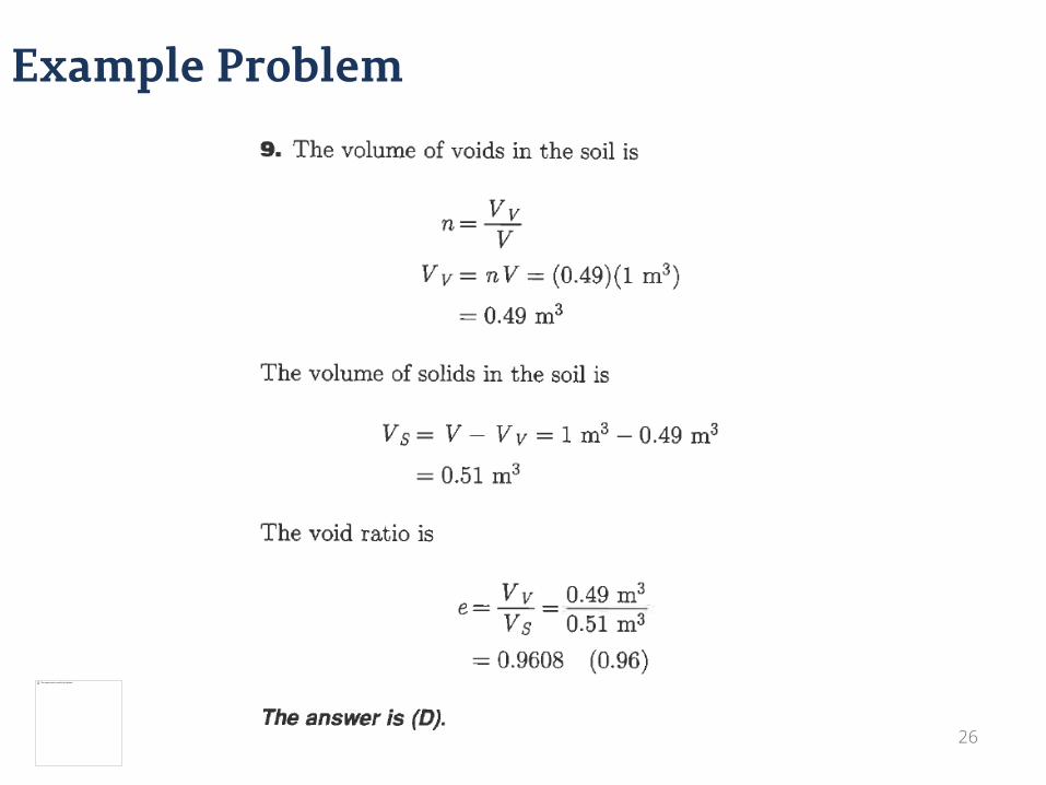
Example Problem

29
This image cannot currently be displayed.
Example Problem

30
This image cannot currently be displayed.
Proctor Test
31
This image cannot currently be displayed.
Proctor Test-Soil Compaction • Compaction
▫ densification of soil by removal of air and rearrangement of soil particles through addition of mechanical energy.
• Energy exerted by compaction forces soil to fill available, and additional frictional forces between the soil particles improves mechanical properties the soil.
• Degree of compaction of a soil ▫ measured by its dry unit weight, γd. ▫ dry unit weight after compaction increases as moisture
content (ω) increases, ▫ after optimum moisture content (ωopt) percentage is
exceeded, any added water will result in a reduction in dry unit weight because pore water pressure (pressure of water in-between each soil particle) will be pushing soil particles apart.

32
This image cannot currently be displayed.
Permeability Tests
Permeability Permeability (hydraulic conductivity) has the same units as velocity Coefficient of permeability is dependent on void ratio, grain-size distribution, pore-size distribution, roughness of mineral particles, fluid viscosity, and degree of saturation. Constant Head Test Difference of head between inlet and outlet remains constant Water collected in a flask is measured in quantity over a time period. More suitable for coarse-grained soils that have a higher coefficient of permeability. Falling Head Test Falling head test uses a similar procedure to the constant head test, but the head is not kept constant. Permeability is measured by decrease in head over a specified time. This test is more appropriate for fine-grained soils.

33
This image cannot currently be displayed.
Permeability or Flow of Water Through Porous Media
K (in in/sec) is the main parameter for flow through soils. There are separate lab tests and equations for sands and clays. • For sands, use the constant head permeameter test with • For clays, use the falling head permeameter test with V is the volume of water used in the test t is the time period over which the test was conducted
7-33 CERC13

Geotechnical Engineering
4/12/2017
FE REVIEW COURSE – SPRING 2017

35
This image cannot currently be displayed.
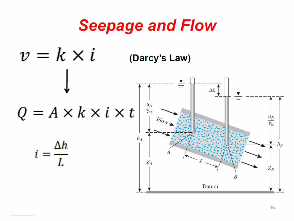
P145 FE Reference Handbook V9.4
36
This image cannot currently be displayed.

37
This image cannot currently be displayed.
Seepage loss through the sandy silt below earth dam (K=3.66 cm/hr)
After B. Muhunthan Washington State University

38
This image cannot currently be displayed.
38

39
This image cannot currently be displayed.
Falling Head Permeability
After Dr. Jerry Vandevelde

40
This image cannot currently be displayed.
After Dr. Jerry Vandevelde

41
This image cannot currently be displayed.
41

42
This image cannot currently be displayed.
Flow Net

43
This image cannot currently be displayed.
Flow Net Components

44
This image cannot currently be displayed.
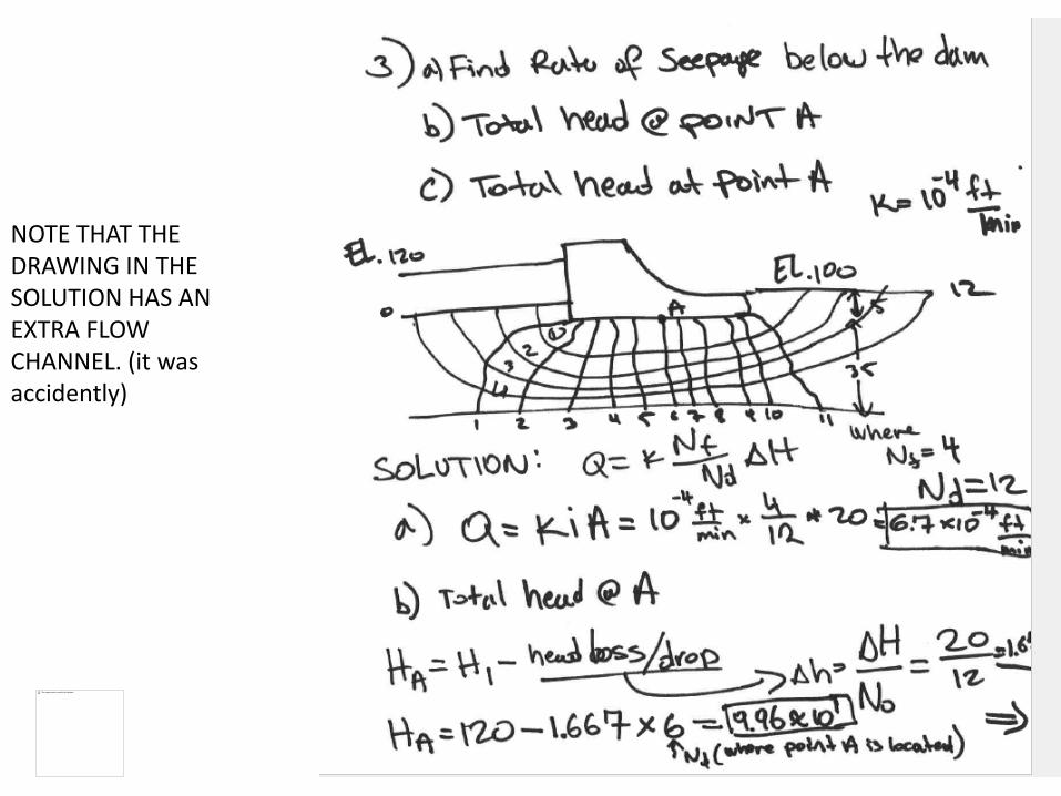
a) What is the rate of seepage (per foot of length) below the dam?
b) What is the total head at Point A?
c) What is the uplift pressure at the bottom of the dam at point A?
A concrete dam is constructed on a fine sand layer, as shown on the figure below. The sand is underlain by impervious bedrock. The sand is 40 feet thick and has a coefficient of permeability of 10-4 ff/min and a saturated unit weight of 122 pounds per cubic foot. The bottom of the dame is 5 feet below the top of the sand layer. The tail water is at the ground surface, elevation 100, and the level of the head water is 120.
After ANUJ CHOUDHARI
45
This image cannot currently be displayed.
45
NOTE THAT THE DRAWING IN THE SOLUTION HAS AN EXTRA FLOW CHANNEL. (it was accidently)

46
This image cannot currently be displayed.
46
47
This image cannot currently be displayed.
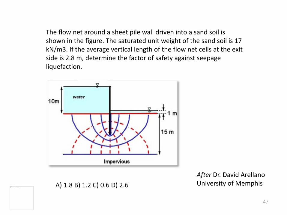
The flow net around a sheet pile wall driven into a sand soil is shown in the figure. The saturated unit weight of the sand soil is 17 kN/m3. If the average vertical length of the flow net cells at the exit side is 2.8 m, determine the factor of safety against seepage liquefaction.
A) 1.8 B) 1.2 C) 0.6 D) 2.6 After Dr. David Arellano University of Memphis

48
This image cannot currently be displayed.
48
P145 FE Reference Handbook V9.4

Geotechnical Engineering
4/12/2017
FE REVIEW COURSE – SPRING 2017

50
This image cannot currently be displayed.
Shear Strength Page 149 in FE Handbook
(psf)
(psf)
is the shear strength

51
This image cannot currently be displayed.
ɸ = 𝒕𝒕𝒕𝒕𝒕𝒕−𝟏𝟏 ( 𝜟𝜟 𝑺𝑺𝑺𝑺𝑺𝑺𝒕𝒕𝑺𝑺 𝑺𝑺𝒕𝒕𝑺𝑺𝑺𝑺𝑺𝑺𝑺𝑺𝜟𝜟 𝑵𝑵𝑵𝑵𝑺𝑺𝑵𝑵𝒕𝒕𝑵𝑵 𝑺𝑺𝒕𝒕𝑺𝑺𝑺𝑺𝑺𝑺𝑺𝑺
)
Reference: Publication No. FHWA NHI-06-088 SOILS AND FOUNDATIONS Reference Manual – Volume I

52
This image cannot currently be displayed.
Direct Shear Test • In the direct shear test, a shear load is applied to a box sample.
7-52 CERC13

53
This image cannot currently be displayed.
Direct Shear Test Example Problem
Hint 1: cohesion = 0
1 1 2 2
Hint 2: solve for ɸ

54
This image cannot currently be displayed.
Solution:

55
This image cannot currently be displayed.
Triaxial Test

56
This image cannot currently be displayed.
Triaxial Test

57
This image cannot currently be displayed.
Triaxial Test Example Problem
effective minor stress, σ3 = 200 kPa
effective major stress,
Lets plot it!
σ1 = 200 kPa + 468 kPa = 668 kPa
σ3 = 200 kPa σ1 = 668 kPa
ɸ= ?
What is the cohesion value (y-intercept?
0 434 kPa
sin ɸ= 234/434
ɸ = 32.6

58
This image cannot currently be displayed.
Unconfined Compressive Strength Test
The unconfined compressive strength test is a triaxial test without the lateral load on the sample. It cannot be used on cohesionless soils.
7-58 CERC13

59
This image cannot currently be displayed.
Unconfined Compressive Strength Example Problem
Hint: The overall volume doesn’t change. Solve for the diameter at failure
See Solutions Set

60
This image cannot currently be displayed.
Solution:

61
This image cannot currently be displayed.
Bearing Capacity Page 149 in FE Handbook
CLAYS (undrained) cohesion > 0 ɸ= 0
SANDS (drained) cohesion = 0 ɸ > = 0
C- ɸ soil cohesion = 500 psf ɸ = 20 deg
Nγ =0
Nq =1.0

62
This image cannot currently be displayed.
Bearing Capacity

63
This image cannot currently be displayed.
Bearing Capacity Page 149 in FE Handbook
One thing to look out for is the ground water elevation
γ’ = γT - γwater
Example Problem: Find the Ultimate Bearing Capacity

64
This image cannot currently be displayed.
Example Problem: Find the Ultimate Bearing Capacity

65
This image cannot currently be displayed.
cohesion = 500 psf
ɸ = 20 deg

66
This image cannot currently be displayed.
Example Problem: Find the Ultimate Bearing Capacity
γ’ = ?
γ’ = γT - γwater
γ’ = 120 pcf – 62.4 pcf = 57.6 pcf
qult = (500 psf * 17.7) + (57.6 pcf * 5’ * 7.4) + (1/2 * 57.6 pcf * 6’ * 5.0)
qult = 11,845.2 psf

67
This image cannot currently be displayed.
Effective Footing Area –Eccentric Loads
Reference: Reference: AASHTO LRFD 2012 Bridge Design Specifications 6th Ed (US)

68
This image cannot currently be displayed.
Shallow Foundations – Example Problem • A shallow rectangular foundation (B= 8 ft, L = 4 ft) transmits an eccentric
load of 95 kips to the soil. What is the Factor of Safety if the ultimate bearing capacity of the soil is 8530 psf? eB = 0.50 ft
eL= 0.25 ft A) 2.9 B) 1.5 C) 2.2 D) 2.5
FOS = Ultimate Bearing Capacity Applied Pressure
Find the Applied Pressure = Force / Effective Area
Effective Area = (B- 2eB ) * (L- 2eL ) = (8’- 2(0.5)) * (4’ - 2(0.25)) = 24.5 ft2
95,000 lbs
Applied Pressure = 95,000 lbs 24.5 ft2 = 3878 psf
FOS = Ultimate Bearing Capacity Applied Pressure
= 8530psf 3878 psf
= 2.2

69
This image cannot currently be displayed.
Consolidation and Settlement Page 147-148 in FE Handbook
Reference: Michael R. Lindeburg, FE Civil Review Manual, 3rd Edition, Professional Publications, Inc.,

70
This image cannot currently be displayed.
Consolidation Tests

71
This image cannot currently be displayed.
Consolidation
Reference: Das, Braja- Principles of Foundation Engineering, 6th Edition

72
This image cannot currently be displayed.
Page 148 in FE Handbook
73
This image cannot currently be displayed.
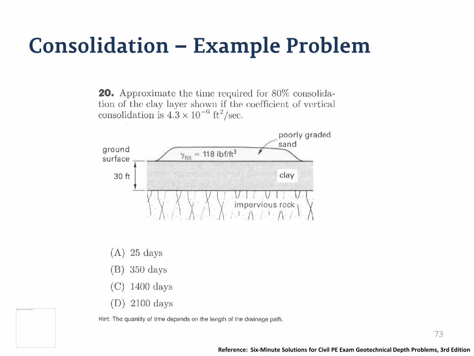
Consolidation – Example Problem
Reference: Six-Minute Solutions for Civil PE Exam Geotechnical Depth Problems, 3rd Edition

74
This image cannot currently be displayed.
Solution:

75
This image cannot currently be displayed.
Consolidation Page 147 in FE Handbook
Calculate the consolidation settlement following the newly constructed embankment. The embankment causes a stress increase of 800 psf at the midpoint of the clay layer
BEDROCK (IMPERVIOUS)
Normally consolidated clay: Unit weight = 120 pcf
Gravel: Unit Weight = 130 pcf
CC=0.4 e0 =0.75
Embankment

76
This image cannot currently be displayed.
Solution:

77
This image cannot currently be displayed.
Pressure at Depth A concentrated vertical load of 6000 lbf is applied at the ground surface. What is the increase in vertical pressure 3.5 ft below the surface and 4 ft from the line of action of the force?
Reference: Civil Engineering Reference Manual for the PE Exam, 15th Edition, Lindeberg
3.5’
4’

78
This image cannot currently be displayed.
Pressure from Applied Loads: Area of Influence
Reference: SOIL MECHANICS (version Fall 2008) Presented by: Jerry Vandevelde, P.E. Chief Engineer GEM Engineering, Inc. 1762 Watterson Trail Louisville, Kentucky
∆σz = 20,000 lbs (8’ + 7’)*(5’+7’)
∆σz = 111.1 psf
79
This image cannot currently be displayed.
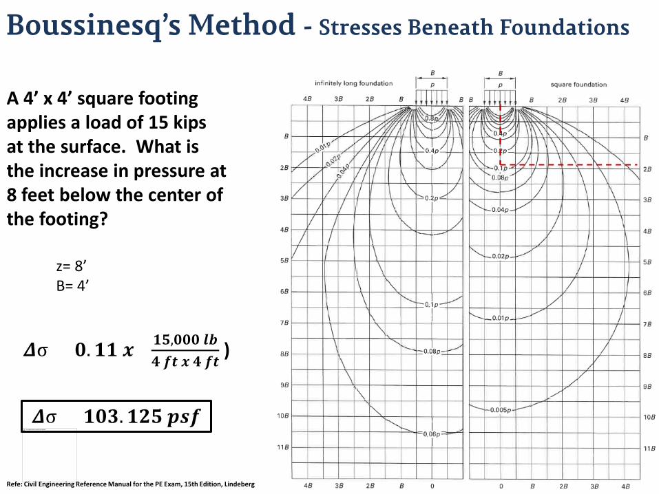
Boussinesq’s Method - Stresses Beneath Foundations
A 4’ x 4’ square footing applies a load of 15 kips at the surface. What is the increase in pressure at 8 feet below the center of the footing?
z= 8’ B= 4’ 𝜟𝜟σ = 𝟎𝟎.𝟏𝟏𝟏𝟏 𝒙𝒙 ( 𝟏𝟏𝟏𝟏,𝟎𝟎𝟎𝟎𝟎𝟎 𝑵𝑵𝒍𝒍
𝟒𝟒 𝒇𝒇𝒕𝒕 𝒙𝒙 𝟒𝟒 𝒇𝒇𝒕𝒕 )
𝜟𝜟σ = 𝟏𝟏𝟎𝟎𝟏𝟏.𝟏𝟏𝟏𝟏𝟏𝟏 𝒑𝒑𝑺𝑺𝒇𝒇
Refe: Civil Engineering Reference Manual for the PE Exam, 15th Edition, Lindeberg

Geotechnical Engineering
4/12/2017
FE REVIEW COURSE – SPRING 2017

81
This image cannot currently be displayed.
Types of Retaining Wall Structures
• There are many different types of walls, but two distinct types:
▫ Fill Retaining Walls ▫ Cut Retaining Walls

82
This image cannot currently be displayed.
Fill Retaining Wall Structures
• For the Exam you will likely see a gravity, semi-gravity, a cantilever, and/or an mechanically stabilized earth (MSE) wall.

83
This image cannot currently be displayed.
Cut Retaining Wall Structures
• Cut wall for the exam would mostly be a soldier pile or anchor wall.

84
This image cannot currently be displayed.
Consideration of Retained Soil
• The two main classifications are cohesive and granular soils.
• Key Concepts:
▫ Cohesive Soils – Clay Type Soils, must account for cohesion in calculations
– C is usually given ,but may have to calculate the cohesion based on the undrained shear strength. In which C=Su=(Undrained Shear Strength (qu)/2)
– Slow Draining ▫ Granular Soils (noncohesive soils or cohensionless soils) – Sand and gravel
type soils, c=0 typically no cohesion or cohesion is negligible.
– Free Draining
• The nature of the backfilled or retained soil greatly affects the design of retaining walls.

85
This image cannot currently be displayed.
Earth Pressure
• Force per unit area exerted by soil on the retaining wall.
• Primarily understood to mean “ Horizontal Earth Pressure” ▫ Active Earth Pressure ▫ Passive Earth Pressure ▫ At-Rest Earth Pressure
• Two Main Theories
▫ Rankine Earth Pressure
– Disregards friction between the soil and the wall. ▫ Coulomb
– Accounts for friction between the soil and the wall.

86
This image cannot currently be displayed.
Rankine’s Earth Pressure
• Civil Engineering (Page 149) • Know how to use this
information given by the FE handbook and be able to determine the horizontal active and passive earth pressure.
• Note that this is for a smooth wall with cohesion-less soil C=0 and a level backfill.

87
This image cannot currently be displayed.
Effective Stress in Retaining Walls
• Above the water table ▫ σv=ɣ(H1) ▫ Where:
– σ is vertical stress, psf (Pa) – ɣ is unit weight of the soil, pcf
(N/m^3) – H is the thickness of the layer, ft.
(m)
• Below the water table ▫ σ’v= σ- μ =(ɣ1(H1))+(ɣ2(H2))- (ɣw(H2)) Or Simplified : ▫ σ’v=ɣ1(H1)+ɣb(H2) ▫ Where:
Ɣb=ɣ-ɣw
Ɣw = 62.4 lbf/ft^3 (9.8 N/m^3)
• Civil Engineering (Page 149) • Must Account for Water Table!

88
This image cannot currently be displayed.
Surcharge in Retaining Walls
• Any additional loading applied externally to the soil is known as surcharge.
• Types of Surcharges: ▫ Point ▫ Line ▫ Uniform (Referenced in NCESS
Handbook) • Unsurcharged pressure plus the
surcharge .
• Does not increase the pore water pressure.
• Civil Engineering (Page 149) • Must Account for Surcharge!

89
This image cannot currently be displayed.
Retaining Wall - Example 1

90
This image cannot currently be displayed.
Retaining Wall - Example 1
• Since the soil is being compressed, the passive earth pressure coefficient is required.
• The passive earth pressure coefficient is
▫ Kp=tan2(45˚+ Φ/2)
▫ Kp=tan2(45˚+ 28˚/2)= 2.77
– Answer: (D) 2.8
• If you got the answer to be (A) you calculated the active earth pressure, which would be correct if there was no force acting on the front of the wall.

91
This image cannot currently be displayed.
Retaining Wall – Example 2
• The Cantilever Retaining Wall shown is under design.
• What is most nearly the active resultant per unit length of the wall? ▫ (A) 280 lbf/ft. ▫ (B) 1900 lbf/ft. ▫ (C) 4300 lbf/ft. ▫ (D) 8500 lbf/ft.

92
This image cannot currently be displayed.
Retaining Wall – Example 2

93
This image cannot currently be displayed.
Retaining Wall – Example 2 (Extended)

94
This image cannot currently be displayed.
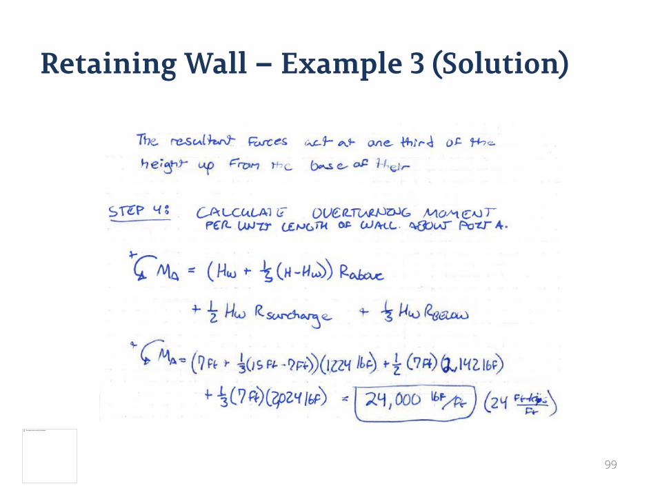
Retaining Wall - Example 3
• After several years of service the drains of the retaining wall from example 2 plugged resulting in a water table 7 foot above the footing level as shown below. Calculate the resulting overturning moment, per unit length of wall, about point A.

95
This image cannot currently be displayed.
Retaining Wall – Example 3 (Solution)

96
This image cannot currently be displayed.
Retaining Wall – Example 3 (Solution)

97
This image cannot currently be displayed.
Retaining Wall – Example 3 (Solution)

98
This image cannot currently be displayed.
Retaining Wall – Example 3 (Solution)
99
This image cannot currently be displayed.
Retaining Wall – Example 3 (Solution)

100
This image cannot currently be displayed.
Slope Failure Resistance

101
This image cannot currently be displayed.
Slope Failure Example
• An excavated slope in uniform soil is shown. The soil has a cohesion of 28.2 kPa and an internal friction angle of 20 degrees, The weight of the soil above the trial failure plane is 5000 kN/m.
• What is most nearly the factor of safety against sliding? ▫ (A) 1.6 ▫ (B) 2.4 ▫ (C) 3.0 ▫ (D) 3.4

102
This image cannot currently be displayed.
Slope Failure Example

103
This image cannot currently be displayed.
Slope Failure Example

Geotechnical Engineering
4/12/2017
FE REVIEW COURSE – SPRING 2017