Embed Size (px)
Citation preview

STATE OF NEW YORKPUBLIC SERVICE COMMISSION
_________________________________________
Case 07-E-0088 - In the Matter of the Adoption )Of an Installed Reserve Margin for the New York )Control Area. )__________________________________________
COMMENTS OF THE NEW YORK STATE RELIABILITY COUNCIL
ON THE INSTALLED RESERVE MARGIN
FOR THE 2013-2014 CAPABILITY YEAR
Michael MagerChairmanNYSRC Executive CommitteeNew York State Reliability CouncilCouch White, LLP540 BroadwayP.O. Box 22222Albany, NY 12201-2222
Dated: January 10, 2013

STATE OF NEW YORKPUBLIC SERVICE COMMISSION
_________________________________________
Case 07-E-0088 - In the Matter of the Adoption )Of an Installed Reserve Margin for the New York )Control Area. )__________________________________________
COMMENTS OF THE NEW YORK STATE RELIABILITY COUNCIL
New York State Reliability Council, LLC (“NYSRC”), through the Chairman of
its Executive Committee, respectfully submits these Comments in Case 07-E-0088. On
December 26, 2012 the New York State Public Service Commission (“Commission”) solicited
comments on whether the Commission should adopt the NYSRC’s Installed Reserve Margin
(“IRM”) of 17.0% for the New York Control Area (“NYCA”) for the Capability Year beginning
on May 1, 2013 and ending on April 30, 2014. The NYSRC respectfully requests that the
Commission consider these comments in support of the NYSRC’s IRM determination for the
2013-2014 Capability Year.
I. SUMMARY
On December 7, 2012, the NYSRC Executive Committee adopted an IRM of
17.0% for the NYCA for the Capability Year beginning on May 1, 2013 and ending April 30,
2014. The Executive Committee’s decision was based on a technical study, the New York
Control Area Installed Capacity Requirements for the Period May 2013 through April 2014,
Technical Study Report (“2013 IRM Study” or “the Study”) and other relevant factors. The
2013 IRM Study is attached to these comments as Exhibit 1. The NYSRC requests that the 2013
IRM Study be made part of the record in this proceeding. Since the 17.0% IRM for the 2013-
2014 Capability Year adopted by the NYSRC represents a change from the 2012-2013 IRM of
16.0%, the NYSRC is required to make an appropriate filing with the Federal Energy Regulatory

2
Commission (“FERC”) under Section 3.03 of the NYSRC Agreement. The NYSRC submitted
its filing to FERC on December 18, 2012 and requested that FERC accept and approve the filing
effective no later than February 15, 2013 so that the revised IRM may be in place for the
installed capacity auction to be conducted by the NYISO on March 28, 2013.1
II. BACKGROUND
Formation and Responsibilities of the NYSRC
The NYSRC was approved by FERC in 1998 as part of the comprehensive
restructuring of the competitive wholesale electricity market in New York State.2 Under the
restructuring, the New York Power Pool (“NYPP”) was replaced by the New York System
Independent System Operator (“NYISO”) as the entity with the primary responsibility for the
reliable operation of the State’s bulk power system. The NYISO also assumed responsibility for
administration of the newly established competitive wholesale electricity markets.
The NYSRC was established to promote and preserve the reliability of the New
York State power system by developing, maintaining and, from time to time, updating the
reliability rules (“Reliability Rules”) that govern the NYISO’s operation of the State’s bulk
power system. The NYSRC develops Reliability Rules in accordance with standards, criteria
and regulations of NERC, NPCC, FERC, the Commission, and the Nuclear Regulatory
Commission.3 The NYISO/NYSRC Agreement provides that the NYISO and all entities
engaged in transactions on the New York State power system must comply with the Reliability
Rules adopted by the NYSRC.4 Compliance with NYSRC Reliability Rules, which are
incorporated into the NYISO’s procedures, are made binding on market participants through the
1 New York State Reliability Council, Docket No. ER 13-572-000 (December 18, 2012).
2 Central Hudson Gas & Electric Corp., et al., 83 FERC ¶ 61,352 (1998).
3 NYISO/NYSRC Agreement, Section 4.1.
4 NYISO/NYSRC Agreement, Section 2.1, 3.1.

3
NYISO’s tariff.5 The NYISO/NYSRC Agreement also assigns to the NYSRC the responsibility
to monitor the NYISO’s compliance with the Reliability Rules and requires the NYISO to
provide the NYSRC the data necessary for it to effectively perform its compliance monitoring
responsibility.6 Each member of the NYSRC Executive Committee is required to have
substantial knowledge and/or expertise in the reliable operation of bulk power electric systems.7
At its inception, the NYSRC adopted the pre-existing NYPP reliability rules.
These planning and operating rules had been developed by the NYPP and the Commission based
on decades of experience in the operation of the New York bulk power system. Revisions to the
Reliability Rules are developed by the NYSRC in an open process with direct participation by
the NYISO and Department of Public Service staff. If the NYSRC and the NYISO should
disagree with respect to a new or modified Reliability Rule, and cannot resolve their differences,
the matter is referred to the Commission for resolution, unless the dispute affects not only
reliability but also matters subject to FERC’s jurisdiction that must be resolved directly by
FERC.8
In addition to incorporating NERC and NPCC reliability criteria, the NYSRC
Reliability Rules include criteria that are more specific or more stringent than NERC and NPCC
criteria that are necessary to meet the special requirements of the NYCA. These special
requirements include the specific electric system characteristics and demographics of New York
State, the complexities related to the maintenance of reliable transmission in New York State
given the configuration of the State’s bulk power system, and the severe consequences that result
from power interruptions in New York State and, in particular, New York City and Long Island.
5 NYISO Market Services Tariff, Sections 5.1, 5.6.
6 NYISO/NYSRC Agreement, Section 3.6.
7 NYSRC Agreement, Section 4.03.
8 NYISO/NYSRC Agreement, Article 5.

4
PSC Support for NYSRC
As noted, the NYSRC was formed as an integral part of the restructuring of the
electricity industry in New York State. It was formed, with the active support of the
Commission, to ensure that the more stringent and mandatory reliability standards in New York
State would be retained under the new competitive wholesale market structure. In its
Supplemental Comments in the FERC proceeding in which the NYSRC Agreement and the
NYISO/NYSRC Agreement were approved, the Commission stated:
PSCNY conditioned its support for the State Reliability Councilupon amendments that would broaden the governance of the[NY]SRC to include more non-utility board members, and tonarrow the responsibilities of the [NY]SRC. The SupplementalFiling appropriately circumscribes the authority of the SRC. Asstated by the utilities, the [NY]SRC would be limited toestablishing reliability rules that tailor the national North AmericanReliability Electric Reliability Council (“NERC”) and regionalNortheast Power Coordinating Council (“NPCC”) standards toNew York State. Consistent with NERC, NPCC, NYPP andNYPSC standards, the [NY]SRC would establish a state-widereserve margin to ensure that adequate generation is available toserve load during normal conditions and system emergencies.
* * *
As proposed, the ISO would implement and enforce the reliabilityrules, not the [NY]SRC. Moreover, the ISO alone would apply thestate-wide resource requirement to set the actual generationresource levels suppliers must meet on different parts of the stategrid. 9
9 Supplemental Comments, State of New York Department of Public Service, Docket Nos. ER 97-1523, et al,(filed May 23, 1997), at 2.

5
NYSRC Establishment of Statewide IRM
One of the most important responsibilities assigned to the NYSRC is the
establishment of the annual statewide installed capacity for the NYCA.10 Section 3.03 of the
NYSRC Agreement reads as follows:
The NYSRC shall establish the state-wide annual installed capacityrequirements for New York State consistent with NERC andNPCC standards. The NYSRC will initially adopt the installedcapacity requirement as set forth in the current NYPP Agreementand currently filed with FERC. Any changes to this requirementwill require an appropriate filing and FERC approval. Inestablishing the state-wide annual installed capacity requirements,consideration will be given to the configuration of the system,generation outage rates, assistance from neighboring systems andLocal Reliability Rules.
The installed capacity requirement is described generally in terms of an installed
reserve margin or IRM.11 The NYISO was assigned the responsibility to determine the installed
capacity obligations of load serving entities (“LSEs”) and to establish locational capacity
requirements needed to ensure that the statewide IRM is met.12 The responsibilities assigned by
the NYSRC Agreement and the NYISO/NYSRC Agreement are implemented in the NYSRC’s
Reliability Rules, the NYSRC’s Policy No. 5-6 and the NYISO’s Market Administration and
Control Area Services Tariff (“Market Services Tariff”). The following is a brief description of
the relevant portions of those documents.
NYSRC Resource Adequacy Criteria
The Introduction to Section A, Resource Adequacy, of the NYSRC Reliability
Rules provides that among the factors to be considered by the NYSRC in setting the annual
10 NYSRC Agreement, § 3.03; NYISO/NYSRC Agreement, § 4.5.
11 The annual statewide ICR is established by implementing Reliability Rules for providing the correspondingstatewide installed reserve margin (“IRM”) requirements. The IRM requirements relates to ICR through thefollowing equation: ICR = (1+ IRM Requirement) x Forecasted NYCA Peak Load (NYSRC Reliability Rules,A. Resource Adequacy, Introduction).
12 NYISO/NYSRC Agreement, § 3.4; NYISO Market Services Tariff, §§ 5.10 and 5.11.4.

6
statewide IRM are the characteristics of the loads, uncertainty in the load forecast, outages and
deratings of generating units, the effects of interconnections to other control areas, and transfer
capabilities within the NYCA.
Reliability Rule A-R1, NYCA Installed Reserve Margin Requirement, provides asfollows:
The NYSRC shall establish the IRM requirement for the NYCAsuch that the probability (or risk) of disconnecting any firm loaddue to resource deficiencies shall be, on average, not more thanonce in ten years. Compliance with this criterion shall beevaluated probabilistically, such that the loss of load expectation(LOLE) of disconnecting firm load due to resource deficienciesshall be on average, no more than 0.1 day per year. Thisevaluation shall make due allowance for demand uncertainty,scheduled outages and deratings, forced outages and deratings,assistance over interconnections with neighboring control areas,NYS Transmission System emergency transfer capability andcapacity and/or load relief from available operating procedures.
Reliability Rule A-R2, Load Serving Entity Installed Capacity, provides that:
LSEs shall be required to procure sufficient resource capacity forthe entire NYISO defined obligation procurement period so as tomeet the statewide IRM requirement determined from A-R1.Further, this LSE capacity obligation shall be distributed so as tomeet locational ICAP requirements, considering the availabilityand capability of the NYS Transmission System to maintain A-R1reliability requirements.
NYSRC Policy No. 5-6, Procedure for Establishing New York Control Area InstalledCapacity Requirements
The last paragraph of Section 1.0, Introduction, of NYSRC Policy No. 5-6
provides that:
The final NYCA IRM requirement, as approved by the NYSRCExecutive Committee, is the basis for various installed capacityanalyses conducted by the NYISO. These NYISO analysesinclude the determination of the capacity obligation of each LoadServing Entity (LSE) on a Transmission District basis, as well asLocational Installed Capacity Requirements, for the followingcapability year. These NYISO analyses are conducted inaccordance with NYSRC Reliability Rules and Procedures.

7
Section 2.2 of NYSRC Policy No. 5-6 provides a timeline for establishing the
statewide IRM. This timeline is based on the NYSRC’s providing the NYISO with the following
year’s NYCA IRM requirement by December 5, when the NYISO, under its installed capacity
and procurement process, is required to begin its studies for determining the following summer’s
LSE capacity obligations.
Section 4.4 of NYSRC Policy No. 5-6 sets forth the process for approval of the
annual statewide IRM by the NYSRC Executive Committee.
4.4 NYSRC Executive Committee
The NYSRC Executive Committee has the responsibility ofapproving the final IRM requirements for the next capability year.
● Review and approve data and modeling assumptions for use in IRM Study; review preliminary base case results.
● Approve sensitivity studies to be run and their results.
● Review and approve final IRM Study prepared by ICS [Installed Capacity Subcommittee].
● Establish and approve the final NYCA IRM requirement for the next capability year (See Section 5).
● To the extent practicable, ensure that the schedule for the above approvals allows that the timeline requirements inSection 2.2 are met.
● Notify the NYISO of the NYCA IRM requirements and meet with NYISO management as required to review IRMStudy results.
● Make IRM requirement study results available to state and federal regulatory agencies and to the general public.
NYISO Market Services Tariff
Relevant portions of Section 5.10 of the NYISO’s Market Services Tariff, NYCA
Minimum Installed Capacity Requirement, read as follows:
The NYCA Minimum Installed Capacity Requirement is derivedfrom the NYCA Installed Reserve Margin, which is establishedeach year by the NYSRC. The NYCA Minimum InstalledCapacity Requirement for the Capability Year beginning each May1 will be established by multiplying the NYCA peak Load

8
forecasted by the ISO by the quantity of one plus the NYCAInstalled Reserve Margin. The ISO shall translate the NYCAInstalled Reserve Margin, and thus the NYCA Minimum InstalledCapacity Requirement, into a NYCA Minimum Unforced CapacityRequirement.
* * *
The NYCA Minimum Unforced Capacity Requirement representsa minimum level of Unforced Capacity that must be secured byLSEs in NYCA for each Obligation Procurement Period. Underthe provisions of this Services Tariff and the ISO Procedures, eachLSE will be obligated to procure its LSE Unforced CapacityObligation.
The first paragraph of Section 5.11.4 of the Market Services Tariff, LSE
Locational Minimum Installed Capacity Requirements, reads as follows:
The ISO will determine the Locational Minimum InstalledCapacity Requirements, stated as a percentage of the Locality’sforecasted Capability Year peak Load and expressed in UnforcedCapacity terms, that shall be uniformly applicable to each LSEserving Load within a Locality. In establishing LocationalMinimum Installed Capacity Requirements, the ISO will take intoaccount all relevant considerations, including the total NYCAMinimum Installed Capacity Requirement, the NYS Power Systemtransmission Interface Transfer Capability, the election by theholder of rights to UDRs that can provide Capacity from anExternal Control Area with a capability year start date that isdifferent from the corresponding ISO Capability Year start date(“dissimilar capability year”), the Reliability Rules and any otherFERC-approved Locational Minimum Installed CapacityRequirements.
III. Adoption of the IRM For 2013-2014 Capability Year
2013 IRM Study
The 2013 IRM Study was conducted by the NYSRC to determine the statewide
IRM necessary to meet NYSRC and NPCC criteria within the NYCA during the period from
May 1, 2013 through April 30, 2014. Computer runs for the 2013 IRM Study were performed by
NYISO staff at the request and under the guidance of the NYSRC. The 2013 IRM Study uses a

9
state-of-the art computer model called the General Electric Multi-Area Reliability Simulation
Program (“GE-MARS”). The GE-MARS model includes a detailed load, generation and
transmission representation of the 11 NYCA zones as well as the four external control areas
(“Outside World Areas”) interconnected to the NYCA. The GE-MARS model calculates the
probability of outages of generating units, coupled with a model of daily peak-hour loads, thus
determining the number of days per year of expected capacity shortages. The resulting measure,
termed the “loss-of-load expectation” (“LOLE”) index, provides a measure of generation system
reliability. This technique is commonly used in the electric power industry for determining
installed reserve requirements.
This 2013 IRM Study employs two study methodologies, the Unified and the IRM
Anchoring Methodologies. These methodologies are discussed in the Study under IRM Study
Procedures, at pages 5 and 6. In addition to calculating NYCA IRM requirement, these
methodologies identify corresponding locational capacity requirements (“LCRs”). In its role of
setting the appropriate LCRs, the NYISO considers the LCR’s identified in the IRM Study. The
2013 IRM Study uses the NYISO’s preliminary peak load forecast for the following summer
period based on the most recent actual summer load conditions. Use of this forecast allows the
NYSRC IRM and NYISO LCR studies to use comparable data.
The 2013 IRM Study also evaluated IRM requirement impacts caused by the
updating of key study assumptions and various sensitivity cases.13 The results of the comparison
with the 2012-2013 IRM are depicted in Table 6-1 at page 20 of the Study. The results of the
sensitivity cases are depicted in Table 7-1 at page 22 of the Study, and Table B-1 at page 73 of
13 The NYSRC Executive Committee approved the assumptions used in the 2013 IRM Study base case on July 13,2012, and approved revised assumptions on November 16, 2012. The sensitivity cases for the 2013 IRM Studywere approved by the NYSRC Executive Committee at its meeting on August 10, 2012. The assumptions usedin the Study are set forth in Appendix A, Table A-3on page 36, Table A-6 on page 40, Table A-8 on page 54,Table A-10 on page 62, and Table A-12 on page 63.

10
the Study. The base case results, the sensitivity cases, and other relevant factors provide the basis
for the NYSRC Executive Committee’s determination to adopt a 17.0% NYCA IRM
requirement for the 2013-2014 Capability Year. Definitions of certain terms in the 2013 IRM
Study can be found in the NYSRC Glossary in Appendix D at page 103 of the Study.
2013 IRM Study Base Case Results
The base case for 2013 IRM Study calculated the NYCA IRM requirement for the
period May 1, 2013 through April 30, 2014 to be 17.1%.14 For the base case, the 2013 IRM
Study also determined LCRs of 83.7% and 102% for New York City and Long Island,
respectively.
The 2013 base case result is 1.0% higher than the 16.1% base case IRM
requirement determined by the 2012 IRM Study. The principal reasons for the increase in the
required IRM are a Special Case Resource (“SCR”) model change, an updated load uncertainty
model, and an updated Outside World Areas model, which together resulted in an increase from
the 2012 base case IRM of 1.6%. The principle driver that decreased the 2013 base case IRM
from the 2012 base case is the new EFORd model, which resulted in a decrease of 0.8%. Table
6-1 of the IRM Study, set forth below, compares the estimated IRM impacts of changing certain
key study assumptions from the 2012 IRM Study.
14 There is a 95% probability that the base case result is within a range of 16.8% to 17.4% based on a standarderror of 0.025 per unit. See Appendix A of the Study, A-1.1 Error Analysis, at 33.

11
Table 0-1 Parametric IRM Impact Comparison (2012 vs. 2013 IRM Study)
ParameterEstimated
IRM Change(%)
IRM (%) Reasons for IRM Changes
2012 IRM Study – Final Base Case 16.12013 Parameters that Increase the IRM
SCR Modeling Change +0.7Model changed from a percent of load
to a fixed value representation.
Updated Load ForecastUncertainty Model
+0.5MWs in the higher bands for Zone J &ROS increased, which increased load
forecast uncertainty.
Updated Outside World Model +0.5 Less emergency assistance from PJM.
Updated Cable Outage Rates +0.4 EFORs for cables increased recently.
Updated Generating UnitEFORd’s
+0.3 Higher fleet EFORd in 2011.
Updated Non-SCR/EDRPEOPs +0.2 83 MW EOP reduction in Downstate.
Updated EDRP Capacity +0.1 Reduced EDRP capacity.
Total IRM Increase +2.72013 Parameters that decrease the IRM
New EFORd Model -0.8Conversion from EFOR to EFORd
lowers IRM.
Hudson Transmission Project -0.4Permits additional assistance from
PJM.
Updated Load Forecast -0.3 Load growth mostly in Upstate.
New Generating Unit andWind Capacity -0.1
Wind capacity is 64 MW less thanassumed in 2012 IRM Study.
Updated SCR Capacity -0.1Reduced SCR capacity outweighs
impact of decreased SCR availability.
Total IRM Decrease -1.72013 Parameters that do not change the IRM
Updated Maintenance 0
Updated Existing GeneratingUnit Capacities
0
Updated Purchases & Sales 0
Retirements 0
Net Change from 2012 Study +1.0
2013 IRM Study Base CaseIRM
17.1

12
After considering the 2013 IRM Study results, the modeling and assumption
changes made to simulate actual operating conditions and system performances, the numerous
sensitivities evaluated, and based on its experience and expertise, on December 7, 2012 the
NYSRC Executive Committee adopted a 17.0% IRM for the 2013-2014 Capability Year. The
NYSRC resolution adopting the IRM is attached to these comments as Exhibit 2.
IV. CONCLUSION
Each year since its inception, the NYSRC has established a statewide annual IRM
requirement that has been implemented by the NYISO. The IRM established by the NYSRC is
used by the NYISO to establish installed capacity requirements for load serving entities in the
NYCA, including LCRs. The IRM is a necessary component of the NYISO’s installed capacity
auctions. The NYISO installed capacity auction for the summer Capability Period is scheduled
for March 28, 2013. The IRM also is used to establish installed capacity prices under the
NYISO installed capacity demand curves. Given the importance of the IRM to the NYISO, load
serving entities, and other NYISO market participants, it is crucial that there be no ambiguity
concerning its level and effectiveness. The 2013 IRM Study is a very thorough and professional
analysis and provides a very sound basis for the IRM adopted by the NYSRC for the 2013-2014
Capability Year.
In its order issued in the proceeding concerning the IRM for the 2012-2013
Capability Year, the Commission stated that “Given its experience and expertise in developing
the IRM, the Commission gives considerable weight to the NYSRC’s findings, conclusions and
recommendations.” 15 It is respectfully submitted that the NYSRC’s IRM policies and
15 Commission Order Adopting Installed Reserve Margin for the New York Control Area for the 2012-2013Capability Year, Case 07-E-0088, Case 05-E-1180, February 17, 2012, at page 9.

13
procedures and the 2013 IRM Study warrant the Commission’s continued confidence and
support.
The NYSRC respectfully recommends, therefore, that the Commission adopt the
NYSRC’s determination that a 17.0% IRM is the appropriate IRM for the New York Control
Area for the Capability Year of May 1, 2013 to April 30, 2014.

EXHIBIT 1
2013 IRM REPORT
New York Control Area Installed Capacity Requirements
For the period May 2013 to April 2014
New York State Reliability Council, LLC
Installed Capacity Subcommittee
Technical Study Report
December 7, 2012

NYSRCNYCA Installed Capacity Requirement for the Period May 2013 through April 2014 Page i
Table of Contents
Executive Summary ....................................................................................................................................... 1
1. Introduction .......................................................................................................................................... 3
2. NYSRC Resource Adequacy Reliability Criterion ................................................................................... 4
3. IRM Study Procedures ........................................................................................................................... 5
4. Study Results – Base Case ..................................................................................................................... 8
5. Models and Key Input Assumptions ..................................................................................................... 8
5.1 Load Model ......................................................................................................................................... 8
5.1.1 Peak Load Forecast ...................................................................................................................... 8
5.1.2 Load Shape Model ....................................................................................................................... 9
5.1.3 Load Forecast Uncertainty (LFU) ................................................................................................ 10
5.2 Capacity Model ................................................................................................................................. 10
5.2.1 Planned Non‐Wind Facilities, Retirements and Reratings ......................................................... 10
5.2.2 Wind Generation ........................................................................................................................ 10
5.2.3 Generating Unit Availability ....................................................................................................... 11
5.2.4 Capacity Availability of Firm Purchases and Sales ..................................................................... 12
5.2.5 Emergency Operating Procedures (EOPs) .................................................................................. 12
5.2.6 Unforced Capacity Deliverability Rights (UDRs) ......................................................................... 14
5.3 Transmission Model .......................................................................................................................... 14
5.3.1 Internal Transmission Model ..................................................................................................... 14
5.4 External Control Area Model ............................................................................................................ 16
5.5 Environmental Initiatives .................................................................................................................. 17
5.6 Database Quality Assurance Reviews ............................................................................................... 18
6. Comparison with 2012 IRM Study Results .......................................................................................... 18
7. Sensitivity Case Study Results ............................................................................................................. 20
8. NYISO Implementation of the NYCA Capacity Requirement .............................................................. 22
8.1 Translation of NYCA ICAP Requirements to UCAP Requirements .................................................... 22
A. Reliability Calculation Models and Assumptions ................................................................................ 29
A.1 GE MARS ........................................................................................................................................... 31
A.2 Methodology .................................................................................................................................... 35

NYSRCNYCA Installed Capacity Requirement for the Period May 2013 through April 2014 Page ii
A.3 Base Case Modeling Assumptions .................................................................................................... 36
A.4 MARS Data Scrub .............................................................................................................................. 66
B. Details for Study Results ..................................................................................................................... 73
B.1 Sensitivity Results ............................................................................................................................. 73
B.2 Environmental Impacts ..................................................................................................................... 76
B.3 Frequency of Implementing Emergency Operating Procedures ...................................................... 82
C. ICAP to UCAP Translation .................................................................................................................... 87
C.1 NYCA and NYC and LI Locational Translations .................................................................................. 88
C.2 Transmission Districts ICAP to UCAP Translation ............................................................................. 92
C.3 Wind Resource Impact on the NYCA IRM and UCAP Markets ........................................................ 100
D. Glossary ............................................................................................................................................. 105
E. Development of Generator Transition Rate Matrices for MARS That Are Consistent with the EFORd Reliability Index ......................................................................................................................................... 111

NYSRCNYCA Installed Capacity Requirement for the Period May 2013 through April 2014 Page iii
Table of Tables & Figures Figure 3‐1 NYCA Load Zones ......................................................................................................................... 5 Figure 3‐2 NYCA Locational Requirements vs. Statewide Requirements ..................................................... 7 Table 6‐1 Parametric IRM Impact Comparison (2012 vs. 2013 IRM Study) ................................................ 20 Table 7‐1 Sensitivity Cases .......................................................................................................................... 22 Figure 8‐1 NYCA Reserve Margins............................................................................................................... 23 Figure A‐1 NYCA ICAP Modeling ................................................................................................................. 29 Table A‐1 Modeling Details ......................................................................................................................... 30 Equation A‐1 ............................................................................................................................................... 32 Equation A‐2 ............................................................................................................................................... 32 Table A‐2 State Transition Rate Example .................................................................................................... 33 Table A‐3 Load Model ................................................................................................................................. 36 Table A‐4 2013 Load Forecast Uncertainty ................................................................................................. 37 Figure A‐2 2013 LFU Distributions .............................................................................................................. 38 Table A‐5 NYCA Peak Load Forecast ........................................................................................................... 39 Table A‐6 Capacity Resources ..................................................................................................................... 40 Table A‐7 Wind Generation ........................................................................................................................ 42 Figure A‐3 NYCA Annual Zonal EFORds ....................................................................................................... 45 Figure A‐4 Five‐Year Zonal EFORds ............................................................................................................. 46 Figure A‐5 NYCA Annual Availability by Fuel ............................................................................................... 47 Figure A‐6 NYCA Five‐Year Availability by Fuel ........................................................................................... 48 Figure A‐7 NERC Annual Availability by Fuel ............................................................................................... 49 Figure A‐8 NERC Five‐Year Availability by Fuel ........................................................................................... 50 Figure A‐9 Planned and Maintenance Outage Rates .................................................................................. 52 Figure A‐10 Scheduled Maintenance .......................................................................................................... 53 Table A‐8 Transmission System Model ....................................................................................................... 54 Table A‐9 Interface Limits Updates ............................................................................................................. 55 Figure A‐11 2013 Transmission Representation ......................................................................................... 58 Figure A‐12 PJM – NY Interface Model ....................................................................................................... 59 Figure A‐13 Full New England Representation ........................................................................................... 60 Table A‐10 External Area Representations ................................................................................................. 62 Table A‐11 Outside World Reserve Margins ............................................................................................... 62 Table A‐12 Assumptions for Emergency Operating Procedures ................................................................. 63 Table A‐13 Emergency Operating Procedures Values ................................................................................ 64 Table A‐14 SCR Performance ...................................................................................................................... 65 Table A‐15 GE MARS Data Scrub ................................................................................................................. 66 Table A‐16 NYISO MARS Data Scrub ........................................................................................................... 69 Table A‐17 Transmission Owner Data Scrub ............................................................................................... 69 Table B‐1 Sensitivity Case Results ............................................................................................................... 73 Table B‐2 Summary of Environmental Programs ........................................................................................ 82

NYSRCNYCA Installed Capacity Requirement for the Period May 2013 through April 2014 Page iv
Table B‐3 Implementation of EOP steps ..................................................................................................... 83 Table C‐1 Historical NYCA Capacity Parameters ......................................................................................... 87 Table C‐2 NYCA ICAP to UCAP Translation .................................................................................................. 89 Table C‐3 New York City ICAP to UCAP Translation .................................................................................... 90 Table C‐4 Long Island ICAP to UCAP Translation ........................................................................................ 91 Table C‐5 Central Hudson Gas & Electric ICAP to UCAP Translation .......................................................... 92 Table C‐6 Con Ed ICAP to UCAP Translation ............................................................................................... 93 Table C‐7 LIPA ICAP to UCAP Translation .................................................................................................... 94 Table C‐8 NGRID ICAP to UCAP Translation ................................................................................................ 95 Table C‐9 NYPA ICAP to UCAP Translation .................................................................................................. 96 Table C‐10 NYSEG ICAP to UCAP Translation .............................................................................................. 97 Table C‐11 O & R ICAP to UCAP Translation ............................................................................................... 98 Table C‐12 RGE ICAP to UCAP Translation .................................................................................................. 99

NYSRCNYCA Installed Capacity Requirement for the Period May 2013 through April 2014 Page 1
Executive Summary A New York Control Area (NYCA) Installed Reserve Margin (IRM) Study is conducted annually by the New York State Reliability Council (NYSRC) Installed Capacity Subcommittee to provide parameters for establishing NYCA IRM requirements for the following capability year. This year’s report covers the period May 2013 to April 2014 (2013 Capability Year).
Results of the NYSRC technical study show that the required NYCA IRM for the 2013 Capability Year is 17.1% under base case conditions.
This study also determined Minimum Locational Capacity Requirements (MLCRs) of 83.7% and 102% for New York City (NYC) and Long Island (LI), respectively. In its role of setting the appropriate locational capacity requirements (LCRs), the New York Independent System Operator (NYISO) will consider these MLCRs.
These study results satisfy and are consistent with NYSRC Reliability Rules, Northeast Power Coordinating Council (NPCC) reliability criteria, and North American Electric Reliability Corporation (NERC) reliability standards.
The 17.1% IRM base case for 2013 represents a 1.0% increase from the 2012 base case IRM of 16.1%. Table 6‐1 shows the IRM impacts of individual study parameters that result in this change. The principle drivers that increased the required IRM are:
A Special Case Resource (SCR) model change An updated load forecast uncertainty model An updated Outside World model
The above IRM drivers together accounted for an IRM increase of 1.7% from the 2012 base case value. Several other updated parameters contributed to an additional 1.0% IRM increase.
In addition, the principle driver that reduced the IRM is a new model that better represents generator performance in reliability analyses. This method calculates an Equivalent Forced Outage Rate during demand (EFORd) that is consistent with the model presently used by the NYISO market. The new EFORd model reduced the IRM by 0.8%. Several other updated parameters contributed to an additional 0.9% IRM decrease.
There are presently five environmental initiatives driven by the State and/or Federal regulators, either in place or are pending, that will affect the operation of most thermal generators in the NYCA, and have the potential to impact future IRM requirements. Compliance with these initiatives could lead to multiple unplanned plant retirements. However, these regulations are

NYSRCNYCA Installed Capacity Requirement for the Period May 2013 through April 2014 Page 2
not expected by themselves to result in retirements that would impact IRM requirements in 2013.
This study also evaluated IRM impacts of 15 sensitivity cases. These results are summarized in Table 7‐1 and in greater detail in Appendix B, Table B‐1. In addition, a confidence interval analysis was conducted to demonstrate that there is a high confidence that the base case 17.1% IRM will fully meet NYSRC and the NPCC resource adequacy criteria.
The base case and sensitivity case IRM results, along with other relevant factors, will be considered in a separate NYSRC Executive Committee process in which the Final NYCA IRM requirement for the 2013 Capability Year is adopted. The 2013 IRM Study also evaluated Unforced Capacity (UCAP) trends. This analysis shows that UCAP margins have steadily decreased over the past six years despite variations in IRM requirements and increases in low capacity factor wind generation.

NYSRCNYCA Installed Capacity Requirement for the Period May 2013 through April 2014 Page 3
1. Introduction This report describes a technical study, conducted by the NYSRC Installed Capacity Subcommittee (ICS), for establishing the NYCA IRM for the period of May 1, 2013 through April 30, 2014 (2013 Capability Year). This study is conducted each year in compliance with Section 3.03 of the NYSRC Agreement which states that the NYSRC shall establish the annual statewide Installed Capacity Requirement (ICR) for the NYCA. The ICR relates to the IRM through the following equation.
1IRM Requirement %
100 1
The base case and sensitivity case study results, along with other relevant factors, will be considered by the NYSRC Executive Committee for its adoption of the Final NYCA IRM requirement for the 2013 Capability Year.
The NYISO will implement the final NYCA IRM as determined by the NYSRC, in accordance with the NYSRC Reliability Rules2 and the NYISO Installed Capacity (ICAP) Manual.3 The NYISO translates the required IRM to an Unforced Capacity (UCAP) basis. These values are also used in a Spot Market Auction based on FERC‐approved Demand Curves. The schedule for conducting the 2013 IRM Study was based on meeting the NYISO’s timetable for these actions.
The study criteria, procedures, and types of assumptions used for this 2013 IRM Study are in accordance with NYSRC Policy 5‐64, Procedure for Establishing New York Control Area Installed Capacity Requirement. The primary reliability criterion used in the IRM study requires a Loss of Load Expectation (LOLE) of no greater than 0.1 days/year for the NYCA. This NYSRC resource adequacy criterion is consistent with NPCC reliability criteria and NERC reliability standards. IRM study procedures include the use of two study methodologies, the Unified and the IRM Anchoring Methodologies. The above reliability criterion and methodologies are discussed in more detail later in the report. In addition to calculating the NYCA IRM requirement, these methodologies identify corresponding MLCRs for NYC and LI. In its role of setting the appropriate LCRs, the NYISO will utilize the same study methodologies and procedures as in the 2013 IRM Study, and will consider the MLCR values determined in this study.
1 For example if the IRM was 17% and the Forecasted NYCA Peak Load was 35,000 then the ICR would equal 40,950. (1+17%/100)*35,000 or 1.17*35000 2 http://www.nysrc.org/NYSRCReliabilityRulesComplianceMonitoring.asp 3 http://www.nyiso.com/public/markets_operations/market_data/icap/index.jsp 4 http://www.nysrc.org/policies.asp

NYSRCNYCA Installed Capacity Requirement for the Period May 2013 through April 2014 Page 4
During 2011 and 2012, a major modeling change for representing generator outage rates was developed and implemented in the 2013 IRM Study. This model calculates an “EFORd,” which is a better measure of generator performance for reliability studies than previously represented. This study improvement is described in the report.
Previous NYCA 2000 to 2012 IRM Study reports can be found on the NYSRC website.5 Table C‐1 in Appendix C provides a comparison of previous NYCA base case and final IRMs for the 2000 through 2012 Capability Years. This table and Figure 8‐1 shows UCAP reserve margin trends over previous years. Definitions of certain terms in this report can be found in the Glossary (Appendix D).
2. NYSRC Resource Adequacy Reliability Criterion The acceptable LOLE reliability level used for establishing NYCA IRM Requirements is dictated by the NYSRC Reliability Rule A‐R1, Statewide Installed Reserve Margin Requirements, which states:
The NYSRC shall establish the IRM requirement for the NYCA such that the probability (or risk) of disconnecting any firm load due to resource deficiencies shall be, on average, not more than once in ten years. Compliance with this criterion shall be evaluated probabilistically, such that the loss of load expectation (LOLE) of disconnecting firm load due to resource deficiencies shall be, on average, no more than 0.1 day per year. This evaluation shall make due allowance for demand uncertainty, scheduled outages and deratings, forced outages and deratings, assistance over interconnections with neighboring control areas, NYS Transmission System emergency transfer capability, and capacity and/or load relief from available operating procedures.
This NYSRC Reliability Rule is consistent with NPCC Resource Adequacy Design Criteria in Section 5.2 of NPCC Directory 1, Design and Operation of the Bulk Power System.
In accordance with NYSRC Rule A‐R2, Load Serving Entity (LSE) Installed Capacity Requirements, the NYISO is required to establish LSE installed capacity requirements, including locational capacity requirements, in order to meet the statewide IRM Requirements established by the NYSRC for maintaining NYSRC Rule A‐R1 above.
5 http://www.nysrc.org/reports3.asp

NYSRCNYCA Installed Capacity Requirement for the Period May 2013 through April 2014 Page 5
3. IRM Study Procedures The study procedures used for the 2013 IRM Study are described in detail in NYSRC Policy 5‐6, Procedure for Establishing New York Control Area Installed Capacity Requirements. Policy 5‐6 also describes the computer program used for reliability calculations and the types of input data and models used for the IRM Study.
This study utilizes a probabilistic approach for determining NYCA IRM requirements. This technique calculates the probabilities of generator unit outages, in conjunction with load and transmission representations, to determine the days per year of expected resource capacity shortages.
General Electric’s Multi‐Area Reliability Simulation (GE‐MARS) is the primary computer program used for this probabilistic analysis. This program includes detailed load, generation, and transmission representation for eleven NYCA zones — plus four external Control Areas (Outside World Areas) directly interconnected to the NYCA. The external Control Areas are: Ontario, New England, Quebec, and the PJM Interconnection. The eleven NYCA zones are depicted in Figure 3‐1 below. GE‐MARS calculates LOLE, expressed in days per year, to provide a consistent measure of system reliability. The GE‐MARS program is described in detail in Appendix A.
Figure 3‐1 NYCA Load Zones
ALBANY
ALLEGANY
BRONX
BROOME
CATTARAUGUS
CAYUGA
CHAUTAUQUA
CHEMUNG
CHENANGO
CLINTON
DELAW ARE
DUTCHESS
ERIE
ESSEX
FRANKLIN
FULTON
GENESEE
GREENE
HERKIMER
JEFFERSON
KINGS
LEW IS
MADISONMONROE
MONTGOMERY
NASSAUNEW YORK
NIAGARA
ONEIDA
ONONDAGA
ONTARIO
ORANGE
ORLEANS
OSW EGO
OTSEGO
PUTNAM
QUEENSRICHMOND
ROCKLAND
ST LAWRENCE
SARATOGA
SCHUYLER
STEUBEN
SUFFOLK
SULLIVAN
TIOGA
TOMPKINS
ULSTER
WARREN
W AYNE
W YOMINGYATES
W EST-
CHES-TER
COLUM-BIA
SCHO-HARIE
W ASH-
ING-
TON
SEN-ECA
HAMILTON
SELAERRENS-
SCHE-NEC-
TADY
CORT-LAND
LIVING-STON
DysingerEast
WestCentral
VolneyEast
MosesSouth
TotalEast
CentralEast
UPNY/SENY
UPNY/CE
MillwoodSouth
DunwoodieSouth
CE-LIPA
A
B
B
C
E
D
F
G
HI
JK
NEW YORK CONTROL AREA
LOAD ZONES

NYSRCNYCA Installed Capacity Requirement for the Period May 2013 through April 2014 Page 6
Using the GE‐MARS program, a procedure is utilized for establishing NYCA IRM requirements (termed the Unified Methodology) which establishes a graphical relationship between NYCA IRM and MLCRs, as illustrated in Figure 3‐2. All points on these curves meet the NYSRC 0.1 days/year LOLE reliability criterion described above. Note that the area above the curve is more reliable than criteria, and vice versa. This methodology develops a pair of curves, one for NYC (Zone J) and one for LI (Zone K). Appendix A of Policy 5‐6 provides a more detailed description of the Unified Methodology.
Base case NYCA IRM requirements and related MLCRs are established by a supplemental procedure (termed the IRM Anchoring Methodology) which is used to define an inflection point on each of these curves. These inflection points are selected by applying a tangent of 45 degrees (Tan 45) analysis at the bend (or “knee”) of each curve. Mathematically, each curve is fitted using a second order polynomial regression analysis. Setting the derivative of the resulting set of equations to minus one yields the points at which the curves achieve the Tan 45 degree inflection point. Appendix B of Policy 5‐6 provides a more detailed description of the methodology for computing the Tan 45 inflection point.

NYSRCNYCA Installed Capacity Requirement for the Period May 2013 through April 2014 Page 7
Figure 3‐2 NYCA Locational Requirements vs. Statewide Requirements
81
82
83
84
85
86
87
88
15 16 17 18 19 20 21
Loca
tiona
l Cap
acity
Req
uire
men
t (%
)
Reserve Margin (%)
New York City
y = 0.2220x2 - 8.5536x + 165.0648 R² = 0.9996
Per Policy 5‐6Calculated IRM =17.1%J LCR = 83.7%
99
100
101
102
103
104
105
106
15 16 17 18 19 20 21
Loca
tiona
l Cap
acity
Req
uire
men
t (%
)
Reserve Margin (%)
Long Island
y = 0.3500x2 - 13.0352x + 222.5125 R² = 0.9999
Per Policy 5‐6Calculated IRM =17.1%K LCR = 102.0%

NYSRCNYCA Installed Capacity Requirement for the Period May 2013 through April 2014 Page 8
4. Study Results – Base Case Results of the NYSRC technical study show that the required NYCA IRM is 17.1% for the 2013 Capability Year under base case conditions. As described above, Figure 3‐2 depicts the relationship between NYCA IRM requirements and resource capacity in NYC and LI.
The tangent points on these curves were evaluated using the Tan 45 analysis. Accordingly, it can be concluded that maintaining a NYCA installed reserve of 17.1% for the 2013 Capability Year, together with MLCRs of 83.7% and 102% for NYC and LI, respectively, will achieve applicable NYSRC and NPCC reliability criteria for the base case study assumptions shown in Appendix A.
Comparing the 2013 MLCR study results to the 2012 IRM Study results (NYC MLCR = 83.9%, LI MLCR = 99.2%), the NYC MLCR decreased by 0.2%, while the LI MLCR increased by 2.8%. The NYISO will consider the various MLCR results when developing the final NYC and LI LCR values for the 2013 Capability Year.
A Monte Carlo simulation error analysis shows that there is a 95% probability that the above base case result is within a range of 16.8% and 17.4% (see Appendix A) when targeting a standard error of 0.025 per unit. This analysis demonstrates that there is a high level of confidence that the base case IRM value of 17.1% is in full compliance with NYSRC and NPCC reliability rules and criteria.
5. Models and Key Input Assumptions This section describes the models and related input assumptions for the 2013 IRM Study. The models represented in the GE‐MARS analysis include a Load Model, Capacity Model, Transmission System Model, and Outside World Model. Potential IRM impacts of pending environmental initiatives are also addressed. The input assumptions for the base case were based on information available prior to October 2012. Appendix A provides more details of these models and assumptions. Table A‐4 compares key assumptions with those used for the 2012 IRM Study.
5.1 Load Model 5.1.1 Peak Load Forecast
A 2013 NYCA summer peak load forecast of 33,278 MW was assumed in the study, a decrease of 57 MW from the 2012 summer peak forecast used in the 2012 IRM Study. The 2013 load forecast, completed by the NYISO staff in collaboration with the NYISO Load Forecasting Task Force, was presented to ICS on October 3, 2012, and considers actual 2012 summer load conditions.

NYSRCNYCA Installed Capacity Requirement for the Period May 2013 through April 2014 Page 9
Use of this 2013 peak load forecast in the 2013 IRM study decreased the IRM by 0.3% compared to the 2012 Study (Table 6‐1). The NYISO will prepare a final 2013 summer forecast in early 2013 for use in the NYISO 2013 Locational Capacity Requirement Study. It is expected that the NYISO’s October 2012 summer peak load forecast for 2013 and the final 2013 forecast will be similar.
5.1.2 Load Shape Model
The 2013 IRM Study was performed using a load shape based on 2002 actual values. This same load shape was used in the six previous IRM studies and is consistent with the load shape assumption used by adjacent NPCC Control Areas. The 2002 load shape has a comparatively larger number of daily peak hours that are close to or nearly equal to the summer peak demand than for other years during the 1999‐2011 period. As a result, there are a higher number of LOLE events using the 2002 load shape than if the load shape based on an average or typical load shape was instead represented. As a result, all else being equal, the resulting IRM will tend to be higher using the 2002 load shape, and therefore represents a conservative IRM load shape representation. To demonstrate this, a sensitivity case was run which replaces the 2002 load shape with a load shape which represents a load shape that is typical of actual load shapes during the 1999‐2011 period (determined to be 2007). This case shows that use of a typical load shape instead of a 2002 load shape would lower the IRM by 2.7% (Table 7‐1).
Because of the conservative nature of the 2002 load shape model, the NYSRC is exploring alternate load shape methodologies for consideration in future IRM studies. One methodology under consideration assigns load shapes to load uncertainty bins. The method develops an index for each year of the available hourly load data for the period 1999 to 2011. The index is developed by taking the 30 highest daily peaks for each year and dividing by the weather adjusted or normalized peak that year to create a per unit value. These 30 per unit values are averaged together to create a single index for each year. The higher the index the more daily peak days there were generally above or closer to the weather adjusted or normalized peak load that year. The index is used to rank order the years and determine their probability of occurrence.

NYSRCNYCA Installed Capacity Requirement for the Period May 2013 through April 2014 Page 10
5.1.3 Load Forecast Uncertainty (LFU)
It is recognized that some uncertainty exists relative to forecasting NYCA loads for any given year. This uncertainty is incorporated in the base case model by using a load forecast probability distribution that is sensitive to different weather conditions. Recognizing the unique LFU of individual NYCA areas, separate LFU models are prepared for four areas: New York City (Zone J), Long Island (Zone K), Westchester (Zones H and I), and the rest of New York State (Zones A‐G).
The load forecast uncertainty models and data used for the 2013 IRM Study were updated by Consolidated Edison for Zones H, I, and J; Long Island Power Authority (LIPA) for Zone K; and the NYISO. Appendix Section A‐3.1 describes these models in more detail. Recognition of load forecast uncertainty in the 2013 IRM Study has an effect of increasing IRM requirements by 9.3% (Table 7‐1). Use of updated LFU models for the 2013 IRM Study increased IRM requirements by 0.5% from the 2012 IRM Study (Table 6‐1).
5.2 Capacity Model 5.2.1 Planned NonWind Facilities, Retirements and Reratings
Planned non‐wind facilities and retirements that are represented in the 2012 IRM Study are shown in Appendix A. The rating for each existing and planned resource facility in the capacity model is based on its Dependable Maximum Net Capability (DMNC). In circumstances where the ability to deliver power to the grid is restricted, the value of the resource is limited to it Capacity Resource Interconnection Service (CRIS) value. The source of DMNC ratings for existing facilities is seasonal tests required by procedures in the NYISO Installed Capacity Manual. Planned non‐wind facilities, retirements, and reratings had no impact on IRM compared to the 2012 IRM Study. Appendix A shows the ratings of all resource facilities that are included in the 2013 IRM Study capacity model.
5.2.2 Wind Generation
It is projected that by the end of the 2013 summer period there will be a total wind capacity of 1,584 MW participating in the capacity market in New York State. All wind farms are located in upstate New York, in Zones A‐E. See Appendix A for details. The 2013 summer period wind capacity projection is

NYSRCNYCA Installed Capacity Requirement for the Period May 2013 through April 2014 Page 11
64 MW lower than the forecast 2012 wind capacity assumed for the 2012 IRM Study.
The 2013 IRM Study base case assumes that the projected 1,584 MW of wind capacity will operate at an 11.0% capacity factor during the summer peak period. This assumed capacity factor is based on an analysis of actual hourly wind generation data collected for wind facilities in New York State during the June through August period, between the hours of 2:00 p.m. and 5:00 p.m. This test period was chosen because it covers the time during which virtually all of the annual NYCA LOLE occurrences are distributed.
The decrease in projected wind capacity from the value of 1,648 MW used in the 2012 IRM Study, to 1,584 MW forecast used for this study, results in a 0.1% IRM decrease (Table 6‐1).
Overall, inclusion of the projected 1,584 MW of wind capacity in the 2013 Study accounts for 4.4% of the 2013 IRM requirement (Table 7‐1). This relatively high IRM impact is a direct result of the very low capacity factor of wind facilities during the summer peak period. The impact of wind capacity on unforced capacity is discussed in Appendix C, Section C.3, “Wind Resource Impact on the NYCA IRM and UCAP Markets.” A detailed summary of existing and planned wind resources is shown in Figure A‐6 of the Appendix.
5.2.3 Generating Unit Availability
Generating unit forced and partial outages are modeled in GE‐MARS by inputting a multi‐state outage model that represents an equivalent forced outage rate during demand periods (EFORd) for each unit represented. Outage data used to determine the EFORd is received by the NYISO from generator owners based on outage data reporting requirements established by the NYISO. Capacity unavailability is modeled by considering the average forced and partial outages for each generating unit that have occurred over the most recent five‐year time period – the time span considered for the 2013 IRM Study covered the 2007‐2011 period. The five‐year EFORd calculated for this period slightly exceeded the 2006‐2010 average value used for the 2012 IRM Study, causing the IRM to increase by 0.3% (Table 6‐1). Figure A‐3 depicts NYCA 2002 to 2011 EFORd trends.
In past NYSRC IRM studies, the model used for calculating loss‐of‐load‐expectation (LOLE) simulated the random outage of generating using

NYSRCNYCA Installed Capacity Requirement for the Period May 2013 through April 2014 Page 12
transition rates developed from the generating availability data system or GADS. GADS is the system that generators use to report their performance. The transition rates calculated from the GADS data have been consistent with NERC’s EFORd definition. The EFORd in practice determines the probability of a generating unit being in a forced outage state during periods of demand. The NYISO capacity market uses the EFORd to determine a generating unit unforced capacity value or UCAP, which determines its overall capacity. The better a generating unit performs, the higher its UCAP.
During 2010, ICS concluded that an improved EFORd model would provide a more accurate measure of generator performance, as well as provide a metric that was aligned with what is used in the capacity markets. An independent consulting firm, Associated Power Analysts (APA), was retained in 2011 by the NYISO to help develop this method. APA proposed and developed two alternative methodologies which would provide transition rate matrices that were consistent with EFORd or probabilities conditioned on demand. After review, ICS selected one of these methodologies to implement for IRM studies. The APA/EFORd methodology was fully developed and successfully validated following extensive testing. ICS then concluded that the new methodology should be implemented for the 2013 IRM Study.
The IRM impact of implementing the APA/EFORd methodology is shown in Table 6‐1 – use of the new model results in a 0.8% lower IRM than use of the previous EFOR model used to represent generator outage rates.
5.2.4 Capacity Availability of Firm Purchases and Sales
The availability of the resources participating in the New York market changes as firm sales and purchases change. Highly available resources acquired through capacity purchases reduce IRM requirements. Similarly, firm external ICAP sales from highly available resources increase the IRM. There is no IRM change from the 2012 Study using updated purchase and sale capacity projections.
5.2.5 Emergency Operating Procedures (EOPs)
(1) Special Case Resources (SCRs)
SCRs are ICAP resources that include loads that are capable of being interrupted on demand and distributed generators that may be activated on demand. This study assumes a SCR base case value of 1,767 MW in July

NYSRCNYCA Installed Capacity Requirement for the Period May 2013 through April 2014 Page 13
2013 with varying amounts during other months based on historical experience.
The SCR performance model is based on an analysis of historical SCR load reduction performance which is described in Section A‐3.7 of Appendix A. Due to the possibility that some of the potential SCR program capacity may not be available during peak periods, projections are discounted for the base case based on previous experience with these programs, as well as any operating limitations. The updated SCR values and performance used for the 2013 IRM Study resulted in a 0.1% IRM decrease from the 2012 IRM Study (Table 6‐1).
The SCR model was changed for the 2013 IRM Study. Previously, the effective value of the program was tied to the individual zonal peaks. To the extent that these peaks were increased to account for load forecast uncertainty, the available amount of SCRs was amplified. SCRs are represented in the 2013 Study by a fixed MW value and are not subject to the model’s amplification for load forecast uncertainty. This model change resulted in an increase of 0.6% from the 2012 IRM study (Table 6‐1).
(2) Emergency Demand Response Programs (EDRP)
EDRP allows registered interruptible loads and standby generators to participate on a voluntary basis – and be paid for their ability to restore operating reserves. The 2013 Study assumes 144 MW of EDRP capacity resources will be registered in 2013, a reduction from 2012. This EDRP capacity was discounted to a base case value of 14 MW reflecting past performance, and is implemented in the study in July and August (differing amounts during other months), while being limited to a maximum of five EDRP calls per month. Both SCRs and EDRP are included in the Emergency Operating Procedure (EOP) model. Unlike SCRs, EDRP are not ICAP suppliers and therefore are not required to respond when called upon to operate. The updated EDRP model used for the 2013 IRM Study resulted in an IRM increase of 0.1% from the 2012 IRM Study (Table 6‐1).
(3) Other Emergency Operating Procedures
In accordance with NYSRC criteria, the NYISO will implement EOPs as required to minimize customer disconnections. Projected 2013 EOP capacity values are based on recent actual data and NYISO forecasts.

NYSRCNYCA Installed Capacity Requirement for the Period May 2013 through April 2014 Page 14
(Refer to Appendix B, Table B‐3, for the expected use of SCRs, EDRP, voltage reductions, and other types of EOPs during 2013.). The updated EOP model, excluding the SCR impact noted above, increased the IRM from the 2012 IRM study by 0.2% (Table 6‐1).
5.2.6 Unforced Capacity Deliverability Rights (UDRs)
The capacity model includes UDRs which are capacity rights that allow the owner of an incremental controllable transmission project to extract the locational capacity benefit derived by the NYCA from the project. Non‐locational capacity, when coupled with a UDR, can be used to satisfy locational capacity requirements. The owner of UDR facility rights designates how they will be treated by the NYSRC and NYISO for resource adequacy studies. The NYISO calculates the actual UDR award based on the performance characteristics of the facility and other data. LIPA’s 330 MW High Voltage Direct Current (HVDC) Cross Sound Cable, 660 MW HVDC Neptune Cable, and the 300 MW Linden Variable Frequency Transformer (VFT) are facilities that are represented in the 2013 IRM Study as having UDR capacity rights. The owners of these facilities have the option, on an annual basis, of selecting the MW quantity of UDRs (ICAP) it plans on utilizing for capacity contracts over these facilities. Any remaining capability on the cable can be used to support emergency assistance which may reduce locational and IRM requirements. The 2013 IRM Study incorporates the elections that these facility owners made for the 2013 Capability Year.
5.3 Transmission Model 5.3.1 Internal Transmission Model
A detailed transmission system model is represented in the GE‐MARS topology. The transmission system topology, which includes eleven NYCA zones and four Outside World Areas, along with transfer limits, is shown in Appendix Figures A‐11, 12, and 13. The transfer limits employed for the 2013 IRM Study were developed from emergency transfer limit analysis included in various studies performed by the NYISO, and from input from Transmission Owners and neighboring regions. The transfer limits are further refined by additional assessments conducted specifically for this cycle of the development of the topology. The assumptions for the transmission model included in the 2013 IRM study are listed in the Appendix in Table A‐7.

NYSRCNYCA Installed Capacity Requirement for the Period May 2013 through April 2014 Page 15
Forced transmission outages are included in the GE‐MARS model for the underground cables that connect New York City and Long Island to surrounding zones. The GE‐MARS model uses transition rates between operating states for each interface, which are calculated based on the probability of occurrence from the failure rate and the time to repair. Transition rates into the different operating states for each interface are calculated based on the circuits comprising each interface, which includes failure rates and repair times for the individual cables, and for any transformer and/or phase angle regulator associated with that particular cable. Updated cable outage rates increased the IRM from the 2012 IRM Study by 0.4% (Table 6‐1).
The interface transfer limits were updated for the 2013 IRM Study based on transfer limit analysis performed for the NYISO 2012 Comprehensive System Planning Process. Transmission Owners and the NYISO performed several analyzes to update several transfer limits. These analyzes are described in detail in Section A.3.3 of Appendix A.
The impact of transmission constraints on NYCA IRM requirements depends on the level of resource capacity in NYC and LI. In accordance with NYSRC Reliability Rule A‐R2, Load Serving Entity ICAP Requirements, the NYISO is required to calculate and establish appropriate LCRs. The most recent NYISO study6 determined that for the 2012 Capability Year, the required LCRs for NYC and LI were 83% and 99%, respectively. A LCR Study for the 2013 Capability Year is scheduled to be completed by the NYISO in January 2013.
Results from 2013 IRM Study were used to illustrate the impact on the IRM requirement for changes of the base case NYC and LI LCR levels of 84% and 102%, respectively. Observations from these results include:
1) Unconstrained NYCA Case
If internal transmission constraints were entirely eliminated the NYCA IRM requirement could be reduced to 15.2%, 1.9% less than the base case IRM requirement (Table 7‐1.) As a result, relieving NYCA transmission constraints would make it possible to reduce the 2013 NYCA installed capacity requirement by approximately 630 MW.
6 Locational Installed Capacity Requirements Study, http://www.nyiso.com/public/markets_operations/services/planning/planning_studies
NYSRCNYCA Installed Capacity Requirement for the Period May 2013 through April 2014 Page 16
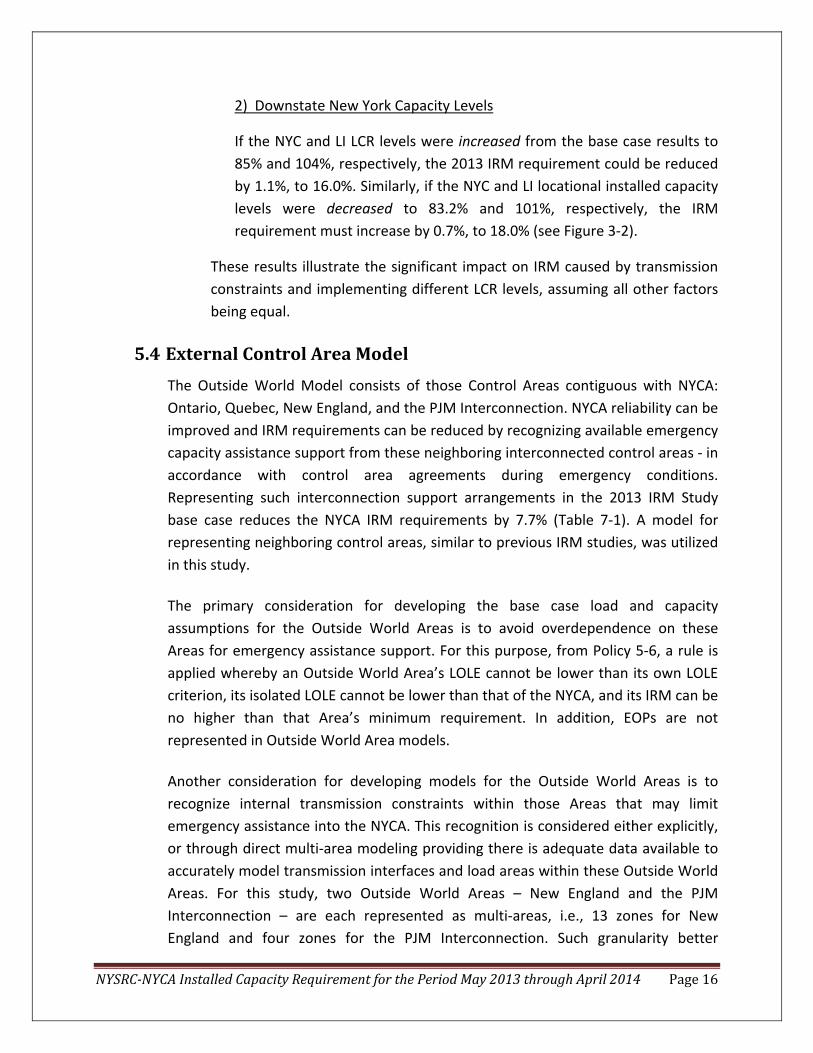
2) Downstate New York Capacity Levels
If the NYC and LI LCR levels were increased from the base case results to 85% and 104%, respectively, the 2013 IRM requirement could be reduced by 1.1%, to 16.0%. Similarly, if the NYC and LI locational installed capacity levels were decreased to 83.2% and 101%, respectively, the IRM requirement must increase by 0.7%, to 18.0% (see Figure 3‐2).
These results illustrate the significant impact on IRM caused by transmission constraints and implementing different LCR levels, assuming all other factors being equal.
5.4 External Control Area Model The Outside World Model consists of those Control Areas contiguous with NYCA: Ontario, Quebec, New England, and the PJM Interconnection. NYCA reliability can be improved and IRM requirements can be reduced by recognizing available emergency capacity assistance support from these neighboring interconnected control areas ‐ in accordance with control area agreements during emergency conditions. Representing such interconnection support arrangements in the 2013 IRM Study base case reduces the NYCA IRM requirements by 7.7% (Table 7‐1). A model for representing neighboring control areas, similar to previous IRM studies, was utilized in this study.
The primary consideration for developing the base case load and capacity assumptions for the Outside World Areas is to avoid overdependence on these Areas for emergency assistance support. For this purpose, from Policy 5‐6, a rule is applied whereby an Outside World Area’s LOLE cannot be lower than its own LOLE criterion, its isolated LOLE cannot be lower than that of the NYCA, and its IRM can be no higher than that Area’s minimum requirement. In addition, EOPs are not represented in Outside World Area models.
Another consideration for developing models for the Outside World Areas is to recognize internal transmission constraints within those Areas that may limit emergency assistance into the NYCA. This recognition is considered either explicitly, or through direct multi‐area modeling providing there is adequate data available to accurately model transmission interfaces and load areas within these Outside World Areas. For this study, two Outside World Areas – New England and the PJM Interconnection – are each represented as multi‐areas, i.e., 13 zones for New England and four zones for the PJM Interconnection. Such granularity better

NYSRCNYCA Installed Capacity Requirement for the Period May 2013 through April 2014 Page 17
captures the impacts of transmission constraints within these areas, particularly on their ability to provide emergency assistance to the NYCA.
The major changes to the NYCA 2013 IRM Study topology from the 2012 Study are:
Volney East up 800 MW to 5675 MW UPNY/CE fixed at 5150 MW, a 450 MW drop from the previous top dynamic rating of 5600 MW
Ontario to NY increasing by 100 MW A drop in the UPNY/SENY interface of 100 MW to a limit of 5150 MW The Central East interface group increase by 250 MW to a limit of 4800 MW Dunwoodie South interface decreasing by 80 MW to a limit of 5210 MW
These changes and other lesser changes are summarized in the Appendix in Table A‐8.
Base case assumptions considered the full capacity of transfer capability from external Control Areas (adjusted for grandfathered contracts) in determining the level of external emergency assistance.
Updated Outside World Area load, capacity, and transmission representations in the 2013 IRM Study results in an IRM increase from the 2012 IRM Study by 0.5% (Table 6‐1).
5.5 Environmental Initiatives Various environmental initiatives driven by the State and/or Federal regulators are either in place or are pending that will affect the operation of the existing fleet. The United States Environmental Protection Agency (USEPA) has promulgated several regulations that will affect most of the thermal generation fleet of generators in NYCA. Similarly, the New York State Department of Environmental Conservation (NYSDEC) has undertaken the development of several regulations that will apply to most of the thermal fleet in New York.
The control technology retrofit requirements of five environmental initiatives are sufficiently broad in application that certain generator owners may need to address the retirement versus retrofit question. These environmental initiatives are: (i) NYSDEC’s Reasonably Available Control Technology for Oxides of Nitrogen (NOx RACT); (ii) Best Available Retrofit Technology (BART) to address regional haze; (iii) Best Technology Available (BTA) for cooling water intake structures; (iv) the USEPA’s

NYSRCNYCA Installed Capacity Requirement for the Period May 2013 through April 2014 Page 18
Mercury and Air Toxics Standards (MATS); and (v) either the Cross State Air Pollution Rule (CSAPR) or its predecessor the Clean Air Interstate Rule (CAIR) addressing interstate transport of criteria air pollutants. Although all but CSAPR are currently in effect, these environmental regulations are not expected by themselves to result in retirements and impact IRM requirements in 2013.
Beyond 2013 as many as 34,000 MW in the existing NYCA generator fleet will have some level of exposure to the new regulations, as further discussed in Appendix B. The magnitude of the combined investments required to comply with the five initiatives could lead to multiple unplanned plant retirements.
5.6 Database Quality Assurance Reviews It is critical that the data base used for IRM studies undergo sufficient review in order to verify its accuracy.
The NYISO, General Electric (GE), and the New York Transmission Owners (TOs) conducted independent data quality assurance reviews after the base case assumptions were developed and prior to preparation of the final base case. Masked and encrypted input data was provided by the NYISO to the transmission owners for their reviews. The NYISO, GE, and TO reviews found several minor data errors, none of which affected IRM requirements in the preliminary base case. The data found to be in error by these reviews were corrected before being used in the final base case studies. A summary of these quality assurance reviews is shown in Appendix A.
6. Comparison with 2012 IRM Study Results The results of this 2013 IRM Study show that the base case IRM result represents a 1.0% increase from the 2012 IRM Study base case value. Table 6‐1 compares the estimated IRM impacts of updating several key study assumptions and revising models from those used in the 2012 Study. The estimated percent IRM change for each parameter in was calculated from the results of a parametric analysis in which a series of IRM studies were conducted to test the IRM impact of individual parameters. The results of this analysis were normalized such that the net sum of the ‐/+ % parameter changes totals the 1.0 % IRM increase from the 2012 Study. Table 6‐1 also provides the reason for the IRM change for each study parameter from the 2012 Study.
The principal drivers shown in Table 6‐1 that increased the required IRM from the 2012 IRM base case are: a SCR model change, an updated load forecast uncertainty model, and an updated Outside World Model, which together, increased the 2012 IRM by 1.6%. The

NYSRCNYCA Installed Capacity Requirement for the Period May 2013 through April 2014 Page 19
principle driver that decreased the required IRM from the 2012 IRM base case is the new EFORd model, which decreased the 2012 IRM by 0.8%.
The parameters in Table 6‐1 are discussed under Models and Key Input Assumptions. A more detailed description of these changes and their IRM impacts can be found in Appendix A.

NYSRCNYCA Installed Capacity Requirement for the Period May 2013 through April 2014 Page 20
Table 6‐1 Parametric IRM Impact Comparison (2012 vs. 2013 IRM Study)
Parameter Estimated IRM Change (%)
IRM (%) Reasons for IRM Changes
2012 IRM Study – Final Base Case 16.1
2013 Parameters that Increase the IRM
SCR Modeling Change +0.7 Model changed from a percent of load
to a fixed value representation.
Updated Load Forecast Uncertainty Model
+0.5 MWs in the higher bands for Zone J & ROS increased, which increased load
forecast uncertainty. Updated Outside World
Model +0.5 Less emergency assistance from PJM.
Updated Cable Outage Rates +0.4 EFORs for cables increased recently.
Updated Generating Unit EFORd’s
+0.3 Higher fleet EFORd in 2011.
Updated Non‐SCR/EDRP EOPs +0.2 83 MW EOP reduction in Downstate.
Updated EDRP Capacity +0.1 Reduced EDRP capacity.
Total IRM Increase +2.7 2013 Parameters that decrease the IRM
New EFORd Model ‐0.8 Conversion from EFOR to EFORd
lowers IRM.
Hudson Transmission Project ‐0.4 Permits additional assistance from
PJM. Updated Load Forecast ‐0.3 Load growth mostly in Upstate. New Generating Unit and
Wind Capacity ‐0.1
Wind capacity is 64 MW less than assumed in 2012 IRM Study.
Updated SCR Capacity ‐0.1 Reduced SCR capacity outweighs
impact of decreased SCR availability. Total IRM Decrease ‐1.7
2013 Parameters that do not change the IRMUpdated Maintenance 0
Updated Existing Generating Unit Capacities
0
Updated Purchases & Sales 0
Retirements 0
Net Change from 2012 Study +1.0
2013 IRM Study Base Case IRM
17.1
7. Sensitivity Case Study Results Determining the appropriate IRM requirement to meet NYSRC reliability criteria depends upon many factors. Variations from the base case will, of course, yield different results.

NYSRCNYCA Installed Capacity Requirement for the Period May 2013 through April 2014 Page 21
Table 7‐1 shows IRM requirement results and related NYC and LI locational capacities for three groups of selected sensitivity cases. Many of these sensitivity case results are important considerations when the NYSRC Executive Committee develops the Final NYCA IRM for 2013. A complete summary of the 15 sensitivity case results shown in Table 7‐1 is depicted in Appendix B, Table B‐2. Table B‐2 also includes a description and explanation of each sensitivity case. Because of the lengthy computer run time needed to utilize the Tan 45 method in IRM studies (see Section 3), this method was not applied for the sensitivity studies in Table 7‐1, except for Case 10. This case, which replaces the 2002 load shape with a 2007 load shape model, utilizes the Tan 45 method because of the interest in this alternate modeling approach. The basis for the 2007 load shape model is described in Appendix Section 5.1.2.

NYSRCNYCA Installed Capacity Requirement for the Period May 2013 through April 2014 Page 22
Table 7‐1 Sensitivity Cases
Case Description IRM (%) % Change from Base
Case NYC LCR (%) LI LCR (%)
0 Base Case 17.1 84 102 Impacts of Major MARS Parameters
1 NYCA isolated 24.8% +7.7 91 107
2 No internal NYCA transmission constraints7
15.2% ‐1.9 0 0
3 No load forecast uncertainty 7.8% ‐9.3 79 94 4 No wind capacity (1,585 MW) 12.7% ‐4.4 85 101 5 No SCRs and EDRPs 16.6% ‐0.5 85 103
Impacts of Base Case Assumption and Model Changes
6 Higher Outside World reserve margins
10.9% ‐6.2 81 96
7 Lower Outside World reserve margins
23.2% +6.1 90 106
8 Higher EFORds 18.6% +1.5 87 102 9 Lower EFORds 16.4% ‐0.7 85 100 10 2007 Load Shape8 14.4% ‐2.7 80 96
11 Retire Indian Point Units 2 and 3
22.1% +5.0 93 110
12 300 MW wheel from Quebec to New England
17.5% +0.4 86 101
13 Limit SCRs to five calls per month per zone
20.2% +3.1 88 104
14 Coal unit retirement scenario9 17.8% +0.7 85 101
15 Unit retirements after the base case assumptions were finalized10
16.7% ‐0.4 85 101
8. NYISO Implementation of the NYCA Capacity Requirement 8.1 Translation of NYCA ICAP Requirements to UCAP Requirements
The NYISO values capacity sold and purchased in the market in a manner that considers the forced outage ratings (UCAP) of individual units. To maintain consistency between the DMNC rating of a unit translated to UCAP and the statewide ICR, the ICR must also be translated to an unforced capacity basis. In the
7 There would be no need to establish locational capacity requirements if there were no internal NYCA transmission constraints. 8 The IRM anchoring (Tan 45) methodology was used for this case. 9 This case assumes the retirement of all coal units (as in the NYISO RNA) due to economic and environmental impacts. 10 These are units that have been actually retired (i.e., Dunkirk), or have announced retirement (i.e., Cayuga) since the 2013 IRM study base case assumptions were approved.

NYSRCNYCA Installed Capacity Requirement for the Period May 2013 through April 2014 Page 23
NYCA, these translations occur twice during the course of each capability year, prior to the start of the summer and winter capability periods.
Additionally, any LCRs in place are also translated to equivalent UCAP values during these periods. The conversion to UCAP essentially translates from one index to another; it is not a reduction of actual installed resources. Therefore, no degradation in reliability is expected. The NYISO employs a translation methodology that converts ICAP requirements to UCAP in a manner that ensures compliance with NYSRC Resource Adequacy Rule A‐R1. The conversion to UCAP provides financial incentives to decrease the forced outage rates while improving reliability.
The increase in wind resources increases the IRM because wind capacity has a much lower peak period capacity factor than traditional resources. On the other hand, there is a negligible impact on the need for UCAP. Figure 8‐1 below illustrates that UCAP reserve margins have steadily decreased over the 2006‐2011 period, despite variations of UCAP requirements. This indicates a lower burden on New York loads over time. Appendix C offers a more detailed explanation.
Figure 8‐1 NYCA Reserve Margins
104.0%
106.0%
108.0%
110.0%
112.0%
114.0%
116.0%
118.0%
120.0%
2006 2007 2008 2009 2010 2011 2012
Res
erve
Mar
gin
Year
New York Control Area Reserve MarginsICAP versus UCAP Margins
Covering the years 2006-2012
ICAP margin (IRM) UCAP margin


NYSRCNYCA Installed Capacity Requirement for the Period May 2013 through April 2014 Page 25
Appendices

NYSRCNYCA Installed Capacity Requirement for the Period May 2013 through April 2014 Page 26

NYSRCNYCA Installed Capacity Requirement for the Period May 2013 through April 2014 Page 27
Appendix A
NYCA Installed Capacity Requirement
Reliability Calculation Models and Assumptions
Description of the GE MARS Program: Load, Capacity, Transmission, Outside World Model, and Assumptions

NYSRCNYCA Installed Capacity Requirement for the Period May 2013 through April 2014 Page 28

NYSRCNYCA Installed Capacity Requirement for the Period May 2013 through April 2014 Page 29
A. Reliability Calculation Models and Assumptions The reliability calculation process for determining the NYCA IRM requirement utilizes a probabilistic approach. This technique calculates the probabilities of outages of generating units, in conjunction with load and transmission models, to determine the number of days per year of expected capacity shortages. The General Electric Multi‐Area Reliability Simulation (GE‐MARS) is the primary computer program used for this probabilistic analysis. The result of the calculation for “Loss of Load Expectation” (LOLE) provides a consistent measure of system reliability. The various models used in the NYCA IRM calculation process are depicted in Figure A‐1 below.
Table A‐1 lists the study parameters in the Figure A‐1 models, the source for the study assumptions, and where in Appendix A the assumptions are described. Finally, section A‐3 compares the assumptions used in the 2012 and 2013 IRM reports.
Figure A‐1 NYCA ICAP Modeling
NYISO Parameters – 11 Zones
GE‐MARS
Ontario, Quebec, New England, PJM Area Parameters
2
Zonal Capacity Models
3
Transmission Capacity Models
6
Zonal Load Uncertainty Models 5
Zonal Load Models
4
Area Capacity Models
8
Interconnection Capacity Models
11
Load Uncertainty Models
10
Area Load Models
9

NYSRCNYCA Installed Capacity Requirement for the Period May 2013 through April 2014 Page 30
Table A‐1 Modeling Details
# Parameter Description Source Reference
Internal NYCA Modeling
1 GE MARS General Electric Multi‐Area
Reliability Simulation Program
Section A‐1
2 11 Zones Load Areas Fig A‐1 NYISO Accounting & Billing Manual
3a Zone Capacity Models
Generator models for each generating in zone
Generator availability Unit ratings
GADS data 2012Gold Book11
Section A‐3.2
3b Emergency Operating
Procedures
Reduces load during emergency conditions to
maintain operating reserves NYISO Section A‐3.5
4 Zone Load Models Hourly loads NYCA load shape
and peak forecasts
Section A‐3.1
5 Load Uncertainty
Model
Account for forecast uncertainty due to weather conditions
Historical data Section A‐3.1
6 Transmission Capacity Model
Emergency transfer limits of transmission interfaces
between zones
NYISO Transmission
Studies Section A‐3.3
External Control Area Modeling
7 Ontario, Quebec, ISONE, PJM Control Area Parameters
See 8‐11 Supplied by External
Control Area
8 External Control Area
Capacity models Generator models in
neighboring Control Areas
Supplied by External
Control Area Section A‐3.4
9 External Control Area
Load Models Hourly loads
Supplied by External
Control Area Section A‐3.4
10 External Control Area Load Uncertainty
Models
Account for forecast uncertainty due to economic conditions
Supplied by External
Control Area Section A‐3.4
11 Interconnection Capacity Models
Emergency transfer limits of transmission interfaces between control areas.
Supplied by External
Control Area Section A‐3.3
11 2012 Load and Capacity Data Report, http://www.nyiso.com/public/markets_operations/services/planning/documents/index.jsp

NYSRCNYCA Installed Capacity Requirement for the Period May 2013 through April 2014 Page 31
A.1 GE MARS As the primary probabilistic analysis tool used for establishing NYCA IRM requirements, the GE‐MARS program includes a detailed load, generation, and transmission representation for 11 NYCA Zones, as well as the four external Control Areas (Outside World Areas) interconnected to the NYCA (see Sections A‐3 and A‐5.6 for a description of these Zones and Outside World Areas).
A sequential Monte Carlo simulation forms the basis for GE‐MARS. The Monte Carlo method provides a fast, versatile, and easily expandable program that can be used to fully model many different types of generation, transmission, and demand‐side options. GE‐MARS calculates the standard reliability indices of daily and hourly LOLE (days/year and hours/year) and Loss of Energy Expectation (LOEE in MWh/year). The use of sequential Monte Carlo simulation allows for the calculation of time‐correlated measures such as frequency (outages/year) and duration (hours/outage). The program also calculates the need for initiating Emergency Operating Procedures (EOPs), expressed in days/year (see Section A‐3.5).
In addition to calculating the expected values for the reliability indices, GE‐MARS also produces probability distributions that show the actual yearly variations in reliability that the NYCA could be expected to experience. In determining NYCA reliability, there are several types of randomly occurring events that must be taken into consideration. Among these are the forced outages of generating units and transmission capacity. Monte Carlo simulation models the effects of such random events. Deviations from the forecasted loads are captured by the use of a load forecast uncertainty model.
Monte Carlo simulation approaches can be categorized as “non‐sequential” and “sequential”. A non‐sequential simulation process does not move through time chronologically or sequentially, but rather considers each hour independent of every other hour. Because of this, non‐sequential simulation cannot accurately model issues that involve time correlations, such as maintenance outages, and cannot be used to calculate time‐related indices such as frequency and duration.
Sequential Monte Carlo simulation (used by GE‐MARS) steps through the year chronologically, recognizing the status of equipment is not independent of its status in adjacent hours. Equipment forced outages are modeled by taking the equipment out of service for contiguous hours, with the length of the outage period being determined from the equipment’s mean time to repair. Sequential simulation can

NYSRCNYCA Installed Capacity Requirement for the Period May 2013 through April 2014 Page 32
model issues of concern that involve time correlations, and can be used to calculate indices such as frequency and duration. It also models transfer limitations between individual areas.
Because the GE‐MARS Program is based on a sequential Monte Carlo simulation, it uses state transition rates, rather than state probabilities, to describe the random forced outages of the thermal units. State probabilities give the probability of a unit being in a given capacity state at any particular time, and can be used if one assumes that the unit’s capacity state for a given hour is independent of its state at any other hour. Sequential Monte Carlo simulation recognizes the fact that a unit’s capacity state in any given hour is dependent on a given state in previous hours and influences its state in future hours. It thus requires additional information that is contained in the transition rate data.
For each unit, a transition rate matrix is input that shows the transition rates to go from each capacity state to each other capacity state. The transition rate from state A to state B is defined as the number of transitions from A to B per unit of time in state A (Equation A‐1).
Equation A‐1
Table A‐2 shows the calculation of the state transition rates from historic data for one year. The Time‐in‐State Data shows the amount of time that the unit spent in each of the available capacity states during the year; the unit was on planned outage for the remaining 760 hours. The Transition Data shows the number of times that the unit transitioned from each state to each other state during the year. The State Transition Rates can be calculated from this data. For example, the transition rate from state 1 to state 2 equals the number of transitions from 1 to 2 divided by the total time spent in state 1 (Equation A‐2).
Equation A‐2
1 210 5,000
0.002

NYSRCNYCA Installed Capacity Requirement for the Period May 2013 through April 2014 Page 33
Table A‐2 State Transition Rate Example
Time in State Data Transition Data
State MW Hours From State
To State 1
To State 2
To State 3
1 200 5000 1 0 10 5 2 100 2000 2 6 0 12 3 0 1000 3 9 8 0
State Transition Rates
From State To State 1 To State 2 To State 3 1 0.000 0.002 0.001 2 0.003 0.000 0.006 3 0.009 0.008 0.000
From the state transition rates for a unit, the program calculates the two important quantities that are needed to model the random forced outages on the unit: the average time that the unit resides in each capacity state, and the probability of the unit transitioning from each state to each other state.
Whenever a unit changes capacity states, two random numbers are generated. The first is used to calculate the amount of time that the unit will spend in the current state; it is assumed that the time in a state is exponentially distributed, with a mean as computed from the transition rates. This time in state is added to the current simulation time to calculate when the next random state change will occur. The second random number is combined with the state transition probabilities to determine the state to which the unit will transition when it leaves its current state. The program thus knows for every unit on the system, its current state, when it will be leaving that state, and the state to which it will go next.
Each time a unit changes state, because of random state changes, the beginning or ending of planned outages, or mid‐year installations or retirements, the total capacity available in the unit's area is updated to reflect the change in the unit's available capacity. This total capacity is then used in computing the area margins each hour.
A.1.1 Error Analysis
An important issue in using Monte Carlo simulation programs such as GE‐MARS is the number of years of artificial history (or replications) that must be created to achieve an acceptable level of statistical convergence in the
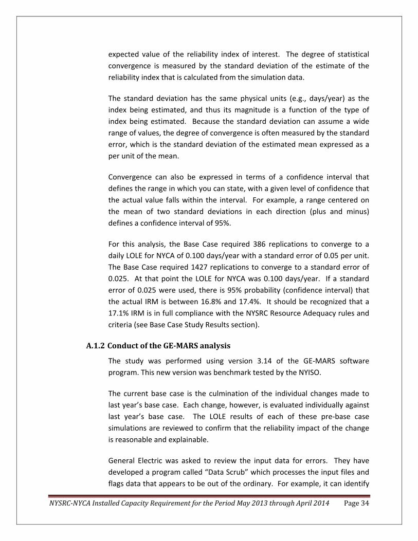
NYSRCNYCA Installed Capacity Requirement for the Period May 2013 through April 2014 Page 34
expected value of the reliability index of interest. The degree of statistical convergence is measured by the standard deviation of the estimate of the reliability index that is calculated from the simulation data.
The standard deviation has the same physical units (e.g., days/year) as the index being estimated, and thus its magnitude is a function of the type of index being estimated. Because the standard deviation can assume a wide range of values, the degree of convergence is often measured by the standard error, which is the standard deviation of the estimated mean expressed as a per unit of the mean.
Convergence can also be expressed in terms of a confidence interval that defines the range in which you can state, with a given level of confidence that the actual value falls within the interval. For example, a range centered on the mean of two standard deviations in each direction (plus and minus) defines a confidence interval of 95%.
For this analysis, the Base Case required 386 replications to converge to a daily LOLE for NYCA of 0.100 days/year with a standard error of 0.05 per unit. The Base Case required 1427 replications to converge to a standard error of 0.025. At that point the LOLE for NYCA was 0.100 days/year. If a standard error of 0.025 were used, there is 95% probability (confidence interval) that the actual IRM is between 16.8% and 17.4%. It should be recognized that a 17.1% IRM is in full compliance with the NYSRC Resource Adequacy rules and criteria (see Base Case Study Results section).
A.1.2 Conduct of the GEMARS analysis
The study was performed using version 3.14 of the GE‐MARS software program. This new version was benchmark tested by the NYISO.
The current base case is the culmination of the individual changes made to last year’s base case. Each change, however, is evaluated individually against last year’s base case. The LOLE results of each of these pre‐base case simulations are reviewed to confirm that the reliability impact of the change is reasonable and explainable.
General Electric was asked to review the input data for errors. They have developed a program called “Data Scrub” which processes the input files and flags data that appears to be out of the ordinary. For example, it can identify

NYSRCNYCA Installed Capacity Requirement for the Period May 2013 through April 2014 Page 35
a unit with a forced outage rate significantly higher than all the others in that size and type category. If something is found, the ISO reviews the data and either confirms that it is correct as is, or institutes a correction. The results of this data scrub are shown in Tables A‐9 through A‐11.
The top three summer peak loads of all Areas external to NYCA are aligned to be on the same days as that of NYCA, even though they may have historically occurred at different times. This is a conservative approach, using the assumption that peak conditions could be the result of a wide spread heat wave. This would result in reducing the amount of assistance that NYCA could receive from the other Areas.
A.2 Methodology The 2013 IRM study continues to use the Unified Methodology that simultaneously provides a basis for the NYCA installed reserve requirements and locational installed capacity requirements. The IRM/LCR characteristic consists of two constituents: 1) a curve function (“the knee of the curve”, and 2) the straight line segments at the asymptotes. The curve function is represented by a quadratic (second order) curve which is the basis for the Tangent 45 inflection point calculation. Consideration of IRM/LCR point pairs remote to the “knee of the curve” may impact the calculation of the quadratic curve function used for the Tangent 45 calculation. The procedure for determining the best fit curve function used for the calculation of the Tangent 45 inflection point to define the base case requirement is based on the following criteria summarized below:
Start with all points on the IRM/LCR curve Develop regression curve equations for all different point to point segments consisting of at least four points
Rank all the regression curve equations based on the R2 value Eliminate those points where the calculated IRM is outside the selected curve point range
Use the highest R2 equation that meets criteria to calculate values for IRM and LCR
Verify that the calculated IRM and corresponding LCR values do not violate the 0.1 LOLE criterion
This approach produces a quadratic curve function with R2 correlation approaching 1.000 as the basis for the Tangent 45 calculation. First derivatives are calculated for

NYSRCNYCA Installed Capacity Requirement for the Period May 2013 through April 2014 Page 36
the NYC and Long Island zones for each of the equations and solved for the 45 degree slope resulting in an average value of 17.1%. The above methodology was adopted by the NYSRC Executive Committee and is incorporated into Policy 5‐6.
A.3 Base Case Modeling Assumptions A.3.1 Load Model
Table A‐3 Load Model
Parameter 2012 Study Assumption
2013 Study Assumption
Explanation
Peak Load
October Forecast: NYCA – 33,335 MW Zone J – 11,607 MW Zone K – 5,521 MW
October Forecast: NYCA – 33,278 MW Zone J – 11,532 MW Zone K – 5,553 MW
Forecast based on examination of 2012
weather normalized peaks. Top three external Area peak days aligned with
NYCA
Load Shape Model 2002 Load Shape 2002 Load Shape The 2002 load shape is still
appropriate
Load Uncertainty Model
Statewide and zonal model updated to reflect current data
Statewide and zonal model updated to reflect
current data
Based on collected data and input from LIPA, Con
Ed, and NYISO. Method and values accepted by LFTF
(1) Peak Load Forecast Methodology
The procedure for preparing the IRM forecast is very similar to that detailed in the NYISO Load Forecasting Manual for the ICAP forecast. The NYISO's Load Forecasting Task Force had three meetings in September 2012 to review analyses prepared by the NYISO of the weather response during the summer. Regional load growth factors (RLGFs) for 2013 were updated by each Transmission Owner based on projections provided to the LFTF in August 2013 by Moody's Analytics. The 2013 forecast was produced by applying the RLGFs to each TO's weather‐normalized peak for the summer of 2012.
The results of the analysis are shown in Table A‐3‐1. The 2012 peak forecast was 33,295 MW (col. 12). The actual peak of 32,457 MW (col. 2) occurred on Tuesday, July 17, 2012. The NYISO activated Special Case Resources (SCRs) in Zone B on that day to curtail load. It is estimated that the impact due to SCRs was 79 MW (col. 3). After accounting for the impacts of weather and the demand response, the weather‐adjusted peak

NYSRCNYCA Installed Capacity Requirement for the Period May 2013 through April 2014 Page 37
load was determined to be 33,118 MW (col. 6), 177 MW (‐0.5%) below the forecast. The Regional Load Growth Factors are shown in column 10. The 2013 forecast for the NYCA is 32,872 MW (col. 11).
The LFTF recommends this forecast to the NYSRC for its use in the 2013 IRM study.
(2) Zonal Load Forecast Uncertainty
For 2013, an updated models were provided by Con‐Ed and LIPA for Zones H&I, J and K. The NYISO developed models for Zones A through G and reviewed the models for the other zones. The results of these models are presented in Table A‐4. Each row represents the probability that a given range of load levels will occur, on a per‐unit basis, by zone. These results are presented graphically in Figure A‐4.
Table A‐4 2013 Load Forecast Uncertainty
Bin No. Probability A ‐ G H & I Zone J Zone K1 0.62% 84.75% 78.93% 84.49% 86.13%2 6.06% 89.67% 85.00% 89.29% 89.96%3 24.17% 94.80% 91.23% 93.97% 94.98%4 38.30% 100.00% 97.41% 98.31% 100.00%5 24.17% 105.14% 103.29% 102.02% 105.02%6 6.06% 110.09% 108.56% 104.81% 110.04%7 0.62% 114.73% 112.89% 106.35% 114.20%
Low ‐ Med 15.3% 18.5% 13.8% 13.9%Hi‐Med 14.7% 15.5% 8.0% 14.2%Delta 30.0% 34.0% 21.9% 28.1%
2013 Load Forecast Uncertainty Models

NYSRCNYCA Installed Capacity Requirement for the Period May 2013 through April 2014 Page 38
Figure A‐2 2013 LFU Distributions
The Consolidated Edison models for Zones H, I & J are based on a peak demand with a 1‐in‐3 probability of occurrence (67th percentile). All other zones are designed at a 1‐in‐2 probability of occurrence of the peak demand (50th percentile). The methodology for determining the LFU models has been reviewed by the NYISO Load Forecasting Task Force.
0%
5%
10%
15%
20%
25%
30%
35%
40%
45%
75% 80% 85% 90% 95% 100% 105% 110% 115% 120%
2013 LFU Distributions
A - G Zone J Zone K H & I

NYSRCNYCA Installed Capacity Requirement for the Period May 2013 through April 2014 Page 39
Table A‐5 NYCA Peak Load Forecast
(1) (2) (3) (4) (5) (6) (7) (8) (10) (11) (12)
Transmission District
2012 Actual MW
2012 Estimated SCR &
Muni Self‐Gen
SCR/EDRP Estimate MW
Weather Adjustment
MW
2012 Weather
Normalized MW
Loss Reallocation
MW
2012 WN MW, Adj for
Losses
Regional Load
Growth Factors
2013 IRM Forecast
2012 ICAP Forecast
Central Hudson 1,121 0 0 12 1,133 ‐8 1,125 1.0040 1,130 1,133.3Con Ed 12,429 75 0 605 13,109 150 13,259 1.0080 13,365 13,430.5LIPA 5,110 30 0 304 5,444 26 5,470 0.9982 5,460 5,508.3NGrid 7,276 50 0 ‐312 7,014 ‐194 6,820 1.0040 6,847 6,749.1NYPA 591 0 0 ‐5 586 8 594 1.0000 594 576.1NYSEG 3,197 0 0 ‐152 3,045 5 3,050 1.0060 3,069 3,126.7O&R 1,056 0 0 77 1,133 5 1,138 1.0060 1,145 1,158.3RG&E 1,677 0 79 ‐103 1,653 8 1,661 1.0040 1,668 1,612.3Grand Total 32,457 155 79 427 33,118 0 33,118 1.0048 33,278 33,294.6
(1) (2) (3) (4) (5) (6) (7) (8) (10) (11) (12)
Locality2012 Actual MW
2012 Estimated SCR &
Muni Self‐Gen
SCR/EDRP Estimate MW
Weather Adjustment
MW
2012 Weather
Normalized MW
Loss Reallocation
MW
2012 WN MW, Adj for
Losses
Regional Load
Growth Factors
2013 IRM Forecast
2012 ICAP Forecast
Zone J ‐ NYC 11,112 0 380 ‐52 11,440 0 11,440 1.0080 11,532 11,500.0Zone K ‐ LI 5,505 30 85 ‐57 5,563 0 5,563 0.9982 5,553 5,525.6
Zone K Non‐Coincident Peak Demand occurred on 6/21/2012, from 4 pm to 5 pm EDT.
NYCA Coincident Peak Demand occurred on 7/17/2012, from 4 pm to 5 pm EDT.Regional Load Growth Factors were provided by Transmission Owners.
Zone J Non‐Coincident Peak Demand occurred on 7/18/2012, from 2 pm to 3 pm EDT.

NYSRCNYCA Installed Capacity Requirement for the Period May 2013 through April 2014 Page 40
A.3.2 Capacity Model
The capacity model includes all NYCA generating units, including new and planned units, as well as units that are physically outside New York State, that have met specific criteria to offer capacity in the New York Control Area. The 2012 Load and Capacity Data Report is the primary data source for these resources. Table A‐6 provides a summary of the capacity resource assumptions in the 2013 IRM study.
Table A‐6 Capacity Resources
Parameter 2012 Study Assumption 2013 Study Assumption Explanation
Generating Unit Capacities
Updated DMNC values per 2011 Gold Book. Use the
minimum of CRIS or DMNC value.
Updated DMNC values per 2012 Gold Book. Use the minimum of CRIS or
DMNC value.
Annual update of the Load & Capacity Data Report
Planned Generator Units
Astoria Energy II ‐ Zone J 576 MW (5/2011)
Bayonne Energy Center Zone J 500 MW (5/2012)
EnXco Solar ‐ Zone K, 13.1 MW (12/12) FIT – Solar ‐ Zone K,
17 MW (6/13)
Based on information in the Load and Capacity Report and from the NYISO RNA Project Tracking Group
Wind Modeling
(1648 MW) Derived from hourly wind data with average Summer Peak
Hour availability factor of approximately 11%
(1,584 MW) Derived from hourly wind data
resulting in an average Summer Peak Hour
availability of approximately 11%
Based on collected hourly wind data. Summer Peak Hour capacity factor based on June 1‐Aug 31, hours
beginning 14‐18
Solar Modeling 38.5 MW of total solar
capacity
Existing 31.5 MW plus forecast 30.1 MW of new units. Output checked against actual hourly
solar data.
Based on collected hourly solar data during summer Peak Hours June 1‐Aug 31, hours beginning 14‐18
Retirements 351 MW of Retirements after publication of the
2011 Gold Book
747 MW of Retirements after publication of the
2012 Gold Book
Forced Outage Rates
5‐year (2006‐10) GADS data. (Those units with less than five years data
could use available representative data.)
5‐year (2007‐11) GADS data. (Those units with less than five years data
could use available representative data.)
Most recent 5‐year period.Includes proxy data for unit(s) that are deemed suspect as part of the
GADS screening process.
Planned Outages Based on schedules
received by NYISO and adjusted for history
Based on schedules received by NYISO and adjusted for history
Updated schedules.

NYSRCNYCA Installed Capacity Requirement for the Period May 2013 through April 2014 Page 41
Parameter 2012 Study Assumption 2013 Study Assumption Explanation
Summer Maintenance
Nominal 50 MW Nominal 50 MW Value based on review of prior year’s data with
adjustment for unit history
Gas Turbine Ambient Derate
Derate based on provided temperature correction
curves.
Derate based on provided temperature correction curves.
Operational history indicates derates in line with manufacturer’s
curves Small Hydro
Derate 45% derate 45% derate No Change
(1) Generating Unit Capacities
The capacity rating for each thermal generating unit is based on its Dependable Maximum Net Capability (DMNC). The source of DMNC ratings are seasonal tests required by procedures in the NYISO Installed Capacity Manual. Additionally, each generating resource has an associated capacity CRIS (Capacity Resource Interconnection Service) value. When the associated CRIS value is less than the DMNC rating, the CRIS value is modeled.
Wind units are rated at their nameplate, or full rated value, in the model. The 2012 NYCA Load and Capacity Report, issued by the NYISO, is the source of those generating units and their ratings included on the capacity model.
(2) Planned Generator Units
Generating units not included the Load and Capacity Data Report but that have met specific criteria for inclusion in the IRM study were also modeled. These include units that went into service after the data report was published or that plan to be in service for the summer 2013 capability period, based upon a signed interconnection agreement (by August 1, 2012). Two new units are included in the 2013 IRM Study:
EnXco Solar ‐ 13.1 MW in zone K.
FIT (Feed‐in‐tariff) Solar ‐ 17 MW in zone K.
(3) Wind Modeling
Wind generators are modeled as hourly load modifiers. The output of each unit varies between 0 and the nameplate value based on wind data

NYSRCNYCA Installed Capacity Requirement for the Period May 2013 through April 2014 Page 42
collected near the plant sites during 2002. The 2002 hourly wind data corresponds to the 2002 hourly load shape also used in the model. Characteristics of this data indicate an overall 30% capacity factor with a capacity factor of approximately 11% during the summer peak hours. A total of 1584 MW of installed capacity associated with wind generators is included in this study. New wind units (215 MW) for the 2013 IRM study include the Marble River Wind Farm ‐215 MW in zone D.
Table A‐7 Wind Generation
(4) Solar Modeling
Solar generators are modeled as hourly load modifiers. The output of each unit varies between 0 MW and the nameplate MW value based on solar data collected near the plant sites. Characteristics of this data indicate an overall 65% capacity factor during the summer peak hours. A total of 61.6 MW of solar capacity was modeled in Zone K that includes:
Facility Name ZoneConnecting
Transmission Owner
NYISO Interconnection
Study Queue Project Number
Projected/ Actual In-
Service Date
New Wind Capacity for
2013 IRM (MW)
Total Wind Capacity for
2013 IRM (MW)
Existing UnitsSteel Wind A National Grid 2007 Jan 20.0Bliss Wind Power A Village of Arcade 173 2008 May 100.5Canandaigua Wind Power C NYSEG 135&199 2008 Jun 125.0Hardscrabble Wind E National Grid 156 2011 Sept 74.0Howard Wind C NYSEG 182 2011 Dec 57.4Wethersfield Wind Power C NYSEG 177 2008 Dec 126.0High Sheldon Wind Farm C NYSEG 144 2009 Feb 112.5Altona Wind Power D NYPA 174 2008 Sept 97.5Chateaugay Wind Power D NYPA 214 2008 Sept 106.5Clinton Wind Power D NYPA 172 & 211 2008 May 100.5Ellenburg Windpark D NYPA 175 2008 May 81.0Munnsville E NYSEG 127A 2007 Aug 34.5Maple Ridge 1 E National Grid 171 2006 Feb 231.0Maple Ridge 2 E National Grid 171 2006 Feb 90.7Madison Wind Power E NYSEG N/A 2000 Sept 11.5Proposed UnitsMarble River Wind Farm 1 and 2 D NYPA 161 & 171 2012 Oct 215.0 215.0
TOTAL CAPACITY - ALL CATEGORIES 215.0 1,583.6

NYSRCNYCA Installed Capacity Requirement for the Period May 2013 through April 2014 Page 43
Existing:
Long Island Solar Farm 31.5 MW
Proposed:
EnXco –Solar 13.1 MW
Feed‐in‐Tariff 17 MW
(5) Retirements
There were seven unit retirements or units mothballed as compared to the 2012 Load and Capacity Data Report. The units include:
Far Rockaway ST4 – 107 MW in Zone K
Glenwood ST4 – 115 MW in Zone K
Glenwood ST5 – 109 MW in Zone K
Montauk Diesel – 6 MW in zone K
Astoria GT 10 – 18 MW in zone J
Astoria GT 11 – 16 MW in zone J
Astoria 4 ‐ 376 MW in zone J
(6) Forced Outages
Performance data for thermal generating units in the model includes forced and partial outages, which are modeled by inputting a multi‐state outage model that is representative of the “equivalent demand forced outage rate” (EFORd) for each unit represented. Generation owners provide outage data to the NYISO using Generating Availability Data System (GADS) data in accordance with the NYISO Installed Capacity Manual. The NYSRC is continuing to use a five‐year historical period for the 2013 IRM Study. Figure A‐3 shows the trend of EFORd for various regions within NYCA. Figure A‐4 shows a rolling 5 year average of the same data.
Figures A‐5 and A‐6 show the availability trends of the NYCA broken out by fuel type.

NYSRCNYCA Installed Capacity Requirement for the Period May 2013 through April 2014 Page 44
The multi‐state model for each unit is derived from five years of historic events if it is available. For units with less than five years of historic events, the available years of event data for the unit is used if it appears to be reasonable. For the remaining years, the unit NERC class‐average data is used.
The unit forced outage states for the majority of the NYCA units were obtained from the five‐year NERC‐GADS outage data collected by the NYISO for the years 2007 through 2011. This hourly data represents the availability of the units for all hours. From this, full and partial outage states and the frequency of occurrence were calculated and put in the required format for input to the GE‐MARS program. Where the NYISO had suspect data for a unit that could not be resolved prior to this study, NERC class average data was substituted for the year(s) of suspect data. Figures A‐7 and A‐8 show the unit availabilities of the entire NERC fleet on an annual and 5‐year historical basis.
The actual method of calculation of the EFORd has been improved as a result of a study done by Associated Power Analysts, Inc. in conjunction with the NYISO and the Installed Capacity Subcommittee. For details on how the calculations are done, refer to a report attached as appendix E, titled “Development of Generator Transition Rate Matrices for MARS That Are Consistent with the EFORd Reliability Index” Dated June 2012.

NYSRCNYCA Installed Capacity Requirement for the Period May 2013 through April 2014 Page 45
Figure A‐3 NYCA Annual Zonal EFORds
0.00%
2.00%
4.00%
6.00%
8.00%
10.00%
12.00%
14.00%
16.00%
2003 2004 2005 2006 2007 2008 2009 2010 2011
Weighted Values for Thermal and Large Hydro Units
K
J
NYCA
A‐E
F‐I

NYSRCNYCA Installed Capacity Requirement for the Period May 2013 through April 2014 Page 46
Figure A‐4 Five‐Year Zonal EFORds
0%
2%
4%
6%
8%
10%
12%
2003‐07 2004‐08 2005‐09 2006‐10 2007‐11
Equivalent Forced Outage Rate
YEAR
Weighted Values for Thermal and Large Hydro Units
K
J
NYCA
A‐E
F‐I

NYSRCNYCA Installed Capacity Requirement for the Period May 2013 through April 2014 Page 47
Figure A‐5 NYCA Annual Availability by Fuel
NYCA EQUIVALENT AVAILABILITYBASED ON NERC-GADS DATA FROM 1999 – 2011
ANNUAL WEIGHTED AVERAGES FOR NUCLEAR, COAL, OIL & GAS, AND COMBUSTION TURBINES
70
75
80
85
90
95
100
PERC
ENT
YEARS
COAL NUCLEAR OIL & GAS COMBUSTION TURBINES

NYSRCNYCA Installed Capacity Requirement for the Period May 2013 through April 2014 Page 48
Figure A‐6 NYCA Five‐Year Availability by Fuel
NYCA EQUIVALENT AVAILABILITYBASED ON NERC-GADS DATA FROM 1999 – 2011
FIVE YEAR WEIGHTED AVERAGE
70
75
80
85
90
95
100
PERC
ENT
YEAR ENDING
COAL NUCLEAR OIL & GAS COMBUSTION TURBINES

NYSRCNYCA Installed Capacity Requirement for the Period May 2013 through April 2014 Page 49
Figure A‐7 NERC Annual Availability by Fuel
NERC EQUIVALENT AVAILABILITYBASED ON NERC-GADS DATA FROM 1999 – 2010
ANNUAL WEIGHTED AVERAGES FOR NUCLEAR, COAL, OIL, GAS, AND COMBUSTION TURBINES
70
75
80
85
90
95
100
PERC
ENT
YEARS
COAL NUCLEAR OIL GAS COMBUSTION TURBINES

NYSRCNYCA Installed Capacity Requirement for the Period May 2013 through April 2014 Page 50
Figure A‐8 NERC Five‐Year Availability by Fuel
NERC EQUIVALENT AVAILABILITYBASED ON NERC-GADS DATA FROM 1999 – 2010
FIVE YEAR WEIGHTED AVERAGE
70
75
80
85
90
95
100
PER
CEN
T
YEAR ENDING
COAL NUCLEAR OIL GAS COMBUSTION TURBINES

NYSRCNYCA Installed Capacity Requirement for the Period May 2013 through April 2014 Page 51
(7) Planned Outages and Summer Maintenance
A second performance parameter to be modeled for each unit is scheduled maintenance. This parameter includes both planned and maintenance outage components. The planned outage component is obtained from the generator owners, and where necessary, extended so that the scheduled maintenance period equals the historic average using the same five year period used to determine EFORd averages. Figure A‐9 provides a graph of scheduled outage trends over the 1992 through 2011 period for the NYCA generators.
Typically, generator owners do not schedule maintenance during the summer peak period. However, it is highly probable that some units will need to schedule maintenance during this period. Each year, the previous five year period is reviewed to determine the scheduled maintenance MW during the previous peak periods. An assumption is determined as to how much to model in the current study. For the 2013 IRM study, a nominal 50 MW of summer maintenance is modeled. The amount is equally divided between upstate and downstate. Figure A‐10 shows the weekly scheduled maintenance for the 2012 IRM study compared to this study.
(8) Gas Turbine Ambient Derate
Operation of combustion turbine units at temperatures above DMNC test temperature results in reduction in output. These reductions in gas turbine and combined cycle capacity output are captured in the GE‐MARS model using deratings based on ambient temperature correction curves. Based on its review of historical 2006 and 2007 data, the NYISO staff has concluded that the existing combined cycle temperature correction curves are still valid and appropriate. These temperature corrections curves, provided by the Market Monitoring Unit of the NYISO, show unit output versus ambient temperature conditions over a range starting at 60 degrees F to over 100 degrees F. Because generating units are required to report their DMNC output at peak or “design” conditions (an average of temperatures obtained at the time of the transmission district previous four like capability period load peaks), the temperature correction for the combustion turbine units is derived for and applied to temperatures above transmission district peak loads.
Review of the simple cycle combustion turbine data, however, has led the NYISO to introduce to the model what is termed a bias. The NYISO plans

NYSRCNYCA Installed Capacity Requirement for the Period May 2013 through April 2014 Page 52
to extend this analysis in the future to include other capacity limited resources. A NYISO report on this analysis, Adjusting for the Overstatement of the Availability of the Combustion Turbine Capacity in Resource Adequacy Studies, dated October 22, 2007, can be found on the NYISO web site.
The derate does not affect all units because many of the new units are capable of generating up to 88 or 94 MW but are limited by permit to 79.9 MW, so they are not impacted by the temperature derating in obtaining an output of 79.9 MW. About one quarter of the existing 3,700 MW of simple cycle Combustion Turbines fall into this category. The accuracy of temperature corrections for all combustion turbines will continue to be evaluated as operational data becomes available.
(9) Hydro derates
The Niagara, St. Lawrence, and Gilboa hydroelectric projects are modeled with a probability capacity model based on historic water flows and unit performance. The remaining approximately 1,000 MW of run of river hydro facilities are simulated in GE‐MARS with availability reduced using a monthly derate with the highest derated values of 45% occurring during the summer months of July and August. These monthly derates are derived using recent historic hydro water conditions.
Figure A‐9 Planned and Maintenance Outage Rates
0%
5%
10%
15%
20%
25%
30%
Perc
ent O
utag
e
Year
New York Control AreaPlanned and Maintenance Outage Rates
(Over the period 1992-2011)
MO PO Total

NYSRCNYCA Installed Capacity Requirement for the Period May 2013 through April 2014 Page 53
Figure A‐10 Scheduled Maintenance
A.3.3 Transmission System Model
A detailed transmission system model is represented in the GE‐MARS topology. The transmission system topology, which includes eleven NYCA zones and four Outside World Areas, along with transfer limits, is shown in Figure A‐11. The transfer limits employed for the 2013 IRM Study were developed from emergency transfer limit analysis included in various studies performed by the NYISO, and from input from Transmission Owners and neighboring regions. The transfer limits are further refined by additional assessments conducted specifically for this cycle of the development of the topology. The assumptions for the transmission model included in the 2013 IRM study are listed in Table A‐8.
Forced transmission outages are included in the GE‐MARS model for the underground cables that connect New York City and Long Island to surrounding zones. The GE‐MARS model uses transition rates between operating states for each interface, which are calculated based on the probability of occurrence from the failure rate and the time to repair.
01,0002,0003,0004,0005,0006,0007,0008,0009,000
10,00011,000
1 3 5 7 9 11 13 15 17 19 21 23 25 27 29 31 33 35 37 39 41 43 45 47 49 51 53
MW
Week
Scheduled MaintenanceFor NYCA Generation
(IRM Studies)
2012 Study Year 2013 Study Year

NYSRCNYCA Installed Capacity Requirement for the Period May 2013 through April 2014 Page 54
Transition rates into the different operating states for each interface are calculated based on the circuits comprising each interface, which includes failure rates and repair times for the individual cables, and for any transformer and/or phase angle regulator associated with that particular cable.
The TOs provided updated transition rates.
The interface transfer limits were updated for the 2013 IRM Study model based on transfer limit analysis performed for the 2012 Comprehensive System Planning Process. LIPA performed analysis to update the dynamic limits associated with the LIPA to Con Ed limits and the Long Island Group interface, which included the LIPA ties to Zone I and Zone J. The analysis was reviewed by NYISO staff and incorporated into the model. The model for the Cross‐Sound Cable was changed for 2013 based on the latest CP‐8 topology. That change was made to more accurately reflect the source of the capacity rights. A model for HTP was developed based on the existing assumptions for a controllable interface with UDRs and associated capacity rights.
Table A‐8 Transmission System Model
Parameter 2012 Study Assumption 2013 Study Assumption Explanation
Interface Limits
Based on 2011 Operating Study, NYISO Voltage
Studies, 2011 Comprehensive Planning Process analysis, ATR, and additional analysis including
interregional planning initiatives
Based on 2012 Operating Study, NYISO Voltage
Studies, 2012 Comprehensive Planning Process analysis, ATR, and additional analysis including
interregional planning initiatives
Changes in transfer limits are reviewed and commented on
by TPAS.
New Transmission Capability
None identified HTP DC controlled tie‐line
and LI upgrades Model updated to reflect new transmission facility.
Transmission Cable Forced Outage
Rate
All Existing Cable EFORs updated on LI and NYC to reflect 5 year history
All existing Cable EFORs updated on LI and NYC to reflect 5 year history
Based on TO analysis
Unforced Capacity Deliverability Rights (UDRs)
No new projected UDRs HTP line used for
emergency assistance.
UDRs awarded to Hudson Transmission Project (HTP). HTP elected to use the line for emergency assistance.
Figure A‐11 shows the system transmission representation for this year’s study. Figure A‐11.1 shows a more detailed representation of the

NYSRCNYCA Installed Capacity Requirement for the Period May 2013 through April 2014 Page 55
interconnections surrounding the PJM/NYCA downstate interface. Finally, Figure A‐11.2 shows the 13 zone New England Representation in more detail.
As can be seen from the figures, the changes made to interface limits are as follows:
Table A‐9 Interface Limits Updates
2012 2013 Delta Interface Forward Reverse Forward Reverse Forward ReverseWest Central 1770/1550/1350 1770/1500/1350 0/‐50/0 Volney East 4875 5675 800 F to G 3450 3475 25 UPNY/CE 5600/5360/5000 5150 ‐450 CE‐LIPA 175 430 175 510 0 80D to HQ 1200 1000 ‐200 D to Cedars 1 167 1 190 0 23A to IESO 1200 1600 1300 1700 100 100D to VT 150 0 0 0 ‐150 UPNY/SENY 5250 5150 ‐100 CE Group 4550 4800 250 LI Sum 1465 285 1465 344 0 59
The increase in the Volney East interface is due to the selection of a limiting facility that is more closely associated with the Volney East interface, as opposed to the Total East interface. The Total East interface limitation is accounted for in the simulation, because the Total East interface is also part of the MARS topology. The highest UPNY/CE interface limit was decreased by 450 MW. The reduction in the voltage limit was the result of increased load in the area, and a reduction of capacity near the interface. Resources located farther away were utilized to increase flow on the interface. Increases in Long Island interface limits were due to the installation of transmission upgrades associated with local generation retirements. In addition, the three dynamic ratings were removed and this single limit is active for all system conditions. The UPNY/SENY interface limit was reduced because a more conservative assumption was adopted regarding the amount of power transfers through NE that loop through the NYCA system. The CE Group (Central East Group) interface was increased by 250 MW due to a change in the assumption of the simultaneous flow pattern across that part of the NYCA system. The higher limit indicates a more balanced power flow split between the Central East interface and the Marcy South transmission corridor, which was confirmed by

NYSRCNYCA Installed Capacity Requirement for the Period May 2013 through April 2014 Page 56
the thermal transfer limit analysis performed for the 2012 RNA, and other studies.

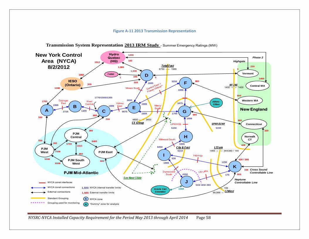
NYSRCNYCA Installed Capacity Requirement for the Period May 2013 through April 2014 Page 58
Figure A‐11 2013 Transmission Representation
DIESO
(Ontario)
PJM West
Connecticut
Vermont
Western MADysinger East
AB
CE
PJM Central
PJM East
Astoria East Generation
2725
1999
1300
1770/1500/1350
800
200 5700
300
200
2650
1600
West Central
1999
5675
Volney East
Hydro Quebec
(HQ)
300
1850
1,0001,500
F
G
H
I
J
Moses South
1600
3250
1999Marcy South
CE Group← 34004800→
1700
3475
1999
Total East0
0
800
800
600
New England
NorwalkCT
330
428 / 388
UPNY/CE
1999
Millwood South
8450
1290530
1999
Neptune Controllable Line
660
660
LI Sum
LI West
510/ 403/ 283
175
428
NY / NE
Cross Sound Controllable Line
330K
Dunwoodie South
External transfer limits1,500
1,500
Grouping used for monitoring
NYCA zonal connections
Standard Grouping
NYCA zonal interfaces
External connections
A NYCA zone
NYCA internal transfer limits
A “Dummy” zone for analysis
Athens-Gilboa
8400
1344
1999
800
Cedars190
1912
UPNY/SENY 5150
1
Central MA
City & East
PJM South West
7500
1015
5500
6500
Highgate
250
Phase 2
1400
PJM Mid-Atlantic
550
550
1300
1700
300
← 19996750 →
← 14001400 →
Transmission System Representation 2013 IRM Study - Summer Emergency Ratings (MW)
New York Control Area (NYCA)
8/2/2012
← 199
99,999 →
5210
4350
1465 → ← 344/260 / 144850
100
1200
5150
See Next Slide

NYSRCNYCA Installed Capacity Requirement for the Period May 2013 through April 2014 Page 59
Figure A‐12 PJM – NY Interface Model
JDummy Zone (J2)
G
PJMEast
Dummy Zone (J3) K
1000/600/500/400
800/320/200
1000
0
1000
1000
660
400
800
660
RECO
500
500
1000
0
1000
Neptune Controllable Line
Joint interface to monitor flow
PJM NYCA
(PJM East to RECO) + (J2 to J) + (PJM East to J3) + (PJM East to J4) = 2000 MWWith the retirement of Hudson 1 and other changes in 2011 PJM RTEP, it was determined that this total interface can be supported to a flow of 2000 MW. This interface grouping contains those interfaces with the Bold hash mark. MARS will distribute this flow accordingly. This will change when additional transmission and generation comes into service in 2014 and 2015 up to 2340.
H
I
1000
A Line + VFT
2012 PJM-SENY MARS Model Draft for discussion only – 5/24/2012
Transmission System Representation 2013 IRM Study - Summer Emergency Ratings (MW)
Dummy Zone (J4)
HTP 660
660

NYSRCNYCA Installed Capacity Requirement for the Period May 2013 through April 2014 Page 60
Figure A‐13 Full New England Representation
Orrington South
Surowiec South
ME - NH
North – South2,700
CSC is not part of this open interface grouping
Norwalk - Stamford1,650 In
RI
Southeast MA
Central MA Northeast MA
226
1,200 S0 W
1,400
0
800800
800
1,2001,150
1,600
0
600
428/388
100
330 (CSC)
Vermont
Rhode Island
Connecticut
Maine
Southern ME
Western MA
Bangor Hydro
Electric
Boston
Southwest CTNorwalk
CTK
G
F
D
Northern District via Phase II
East – West2,800
New Hampshire
Montreal via Highgate
SEMA Export9,999
SWCT Import3,200 In
Connecticut2,500 In
1,400 S1,400 W
1,400 S1875 W
Boston Import4,900
SEMA- RI Export3,000
Total NY- NE(Excludes CSC)
NYCA Zones
Figure A-11.2NEPOOLSystem
Transmission System Representation 2013 IRM Study - Summer Emergency Ratings (MW) – August 1, 2012
K1

NYSRCNYCA Installed Capacity Requirement for the Period May 2013 through April 2014 Page 61
A.3.4 External Area Representations
NYCA reliability largely depends on emergency assistance from its interconnected Control Areas in NPCC and PJM, based on reserve sharing agreements with the Outside World Areas. Load and capacity models of the Outside World Areas are therefore represented in the GE‐MARS analyses. The load and capacity models for New England, Ontario, PJM, and Quebec are based on data received from the Outside World Areas, as well as NPCC sources.
The primary consideration for developing the final load and capacity models for the Outside World Areas is to avoid over‐dependence on the Outside World Areas for emergency capacity support. For this purpose, a rule is applied whereby either an Outside World Area’s LOLE cannot be lower than 0.100 days/year LOLE, or its isolated LOLE cannot be lower than that of the NYCA. In other words, the neighboring Areas are assumed to be equally or less reliable than NYCA. Another consideration for developing models for the Outside World Areas is to recognize internal transmission constraints within the Outside World Areas that may limit emergency assistance to the NYCA. This recognition is considered implicitly for those Areas that have not supplied internal transmission constraint data.
The year 2002 is used in this study for both the NYCA and the Outside World Area load shapes. In order to avoid over‐dependence from emergency assistance, the three highest summer load peak days of the Outside World Areas’ are modeled to match the same load sequence as NYCA.
For this study, both New England and PJM continue to be represented as multi‐area models, based on data provided by these Control Areas.
The EOPs were removed from the Outside World Areas to avoid the difficulty in modeling the sequence and coordination of implementing them. This is a conservative measure.
The assistance from Reliability First Corporation (RFC), with the exception of PJM Mid Atlantic, and the Maritime Provinces was not considered, therefore, limiting the emergency assistance to the NYCA from the immediate neighboring control areas. This consideration is another measure of conservatism added to the analyses.

NYSRCNYCA Installed Capacity Requirement for the Period May 2013 through April 2014 Page 62
The load forecast uncertainty model for the outside world model was supplied from the external Control Areas.
Modeling of the neighboring Control Areas in the base case in accordance with Policy 5‐6 is as follows:
Table A‐10 External Area Representations
Parameter 2012 Study Assumption 2013 Study Assumption Explanation
Capacity Purchases
Grandfathered amounts of 50 MW from NE, 1080 MW from PJM and 1,090 MW from Quebec. All contracts modeled as equivalent
contracts
Grandfathered amounts: ISONE – 50 MW (through
12/2013) PJM – 1080 MW HQ – 1090 MW
All contracts modeled as equivalent contracts
Grandfathered Rights, ETCNL, and other FERC identified
rights.
Capacity Sales Long term firm sales of 279
MW) Long term firm sales of 283
MW (nominal value) These are long term federally
monitored contracts.
Capacity Wheels None modeled. A sensitivity
case may be run None modeled. A sensitivity
case will be run
The ISO tariff is silent about capacity wheels through
NYCA
External Area Modeling
Single Area representations for Ontario and Quebec.
Four zones modeled for PJM. Thirteen zones modeled for
New England
Single Area representations for Ontario and Quebec. Four zones modeled for PJM. Thirteen zones
modeled for New England
The load and capacity data is provided by the neighboring Areas. This updated data may then be adjusted as described in Policy 5
Reserve Sharing All NPCC Control Areas have indicated that they will share reserves equally among all
All NPCC Control Areas have indicated that they will share reserves equally
among all
Per NPCC CP‐8 working group assumption
Table A‐11 Outside World Reserve Margins
Area 2012 Study
Reserve Margin 2013 Study Reserve
Margin 2012 Study LOLE (Days/Year)
2013 Study LOLE (Days/Year)
Quebec 21.8% 24.1%* 0.101 0.100
Ontario 8.4% 13.1% 0.102 0.103
PJM‐Mid‐Atlantic 19.2% 11.2% 0.330 0.425
New England 8.3% 12.3% 0.158 0.104
*This is the summer margin; the winter margin is 0.6%
Table A‐10, above, shows the final reserve margins and LOLEs for the Control Areas external to NYCA.
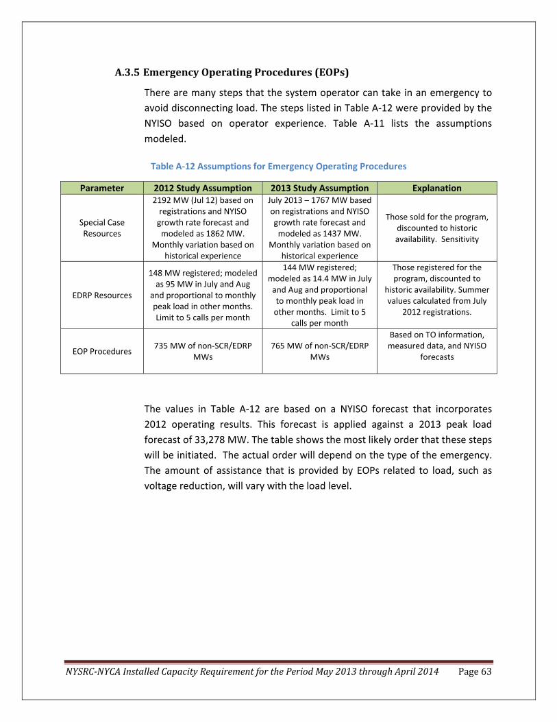
NYSRCNYCA Installed Capacity Requirement for the Period May 2013 through April 2014 Page 63
A.3.5 Emergency Operating Procedures (EOPs)
There are many steps that the system operator can take in an emergency to avoid disconnecting load. The steps listed in Table A‐12 were provided by the NYISO based on operator experience. Table A‐11 lists the assumptions modeled.
Table A‐12 Assumptions for Emergency Operating Procedures
Parameter 2012 Study Assumption 2013 Study Assumption Explanation
Special Case Resources
2192 MW (Jul 12) based on registrations and NYISO growth rate forecast and modeled as 1862 MW.
Monthly variation based on historical experience
July 2013 – 1767 MW based on registrations and NYISO growth rate forecast and modeled as 1437 MW.
Monthly variation based on historical experience
Those sold for the program, discounted to historic availability. Sensitivity
EDRP Resources
148 MW registered; modeled as 95 MW in July and Aug
and proportional to monthly peak load in other months. Limit to 5 calls per month
144 MW registered; modeled as 14.4 MW in July and Aug and proportional to monthly peak load in other months. Limit to 5
calls per month
Those registered for the program, discounted to
historic availability. Summer values calculated from July
2012 registrations.
EOP Procedures 735 MW of non‐SCR/EDRP
MWs 765 MW of non‐SCR/EDRP
MWs
Based on TO information, measured data, and NYISO
forecasts
The values in Table A‐12 are based on a NYISO forecast that incorporates 2012 operating results. This forecast is applied against a 2013 peak load forecast of 33,278 MW. The table shows the most likely order that these steps will be initiated. The actual order will depend on the type of the emergency. The amount of assistance that is provided by EOPs related to load, such as voltage reduction, will vary with the load level.

NYSRCNYCA Installed Capacity Requirement for the Period May 2013 through April 2014 Page 64
Table A‐13 Emergency Operating Procedures Values
Parameter 2012 Study Assumption 2013 Study Assumption Explanation
1
Special Case Resources (SCRs)
Load relief 1767 MW* (based
on sales)
2
Emergency Demand Response
Programs (EDRPs).
Load relief
144/14 MW**
3
5% manual voltage Reduction Load relief 65 MW
4
Thirty‐minute reserve to zero Allow operating reserve to decrease to largest unit capacity (10‐minute reserve)
655 MW
5
5% remote voltage Reduction Load relief 479 MW***
6
Voluntary industrial
curtailment
Load relief
125 MW***
7
General public appeals Load relief 88 MW
8
Emergency Purchases Load relief Varies
9
Ten‐minute reserve to zero Allow 10‐minute reserve to decrease to
zero
1310 MW
10
Customer disconnections Load relief As needed
* The SCR’s are modeled as monthly values. The value for July is 1767 MW. ** The EDRPs are modeled as 144 MW discounted to 14 MW in July and August and further discounted in other
months. They are limited to 5 calls a month. *** These EOPs are modeled in the program as a percentage of the hourly peak. The associated MW value is based
on a forecast 2012 peak load of 33,278 MW.
A.3.6 Location Capacity Requirements
The GE‐MARS model used in the IRM study provides an assessment of the adequacy of the NYCA transmission system to deliver assistance from one Zone to another for meeting load requirements. Previous studies have identified transmission constraints into certain Zones that could impact the LOLE of these Zones, as well as the statewide LOLE. To minimize these potential LOLE impacts, these Zones require a minimum portion of their NYCA ICAP requirement, i.e., locational ICAP, which shall be electrically located within the Zone in order to ensure that sufficient energy and capacity are available in that Zone and that NYSRC Reliability Rules are met. Locational ICAP requirements are currently applicable to two transmission‐constrained Zones, New York City and Long Island, and are normally expressed as a percentage of each Zone’s annual peak load.
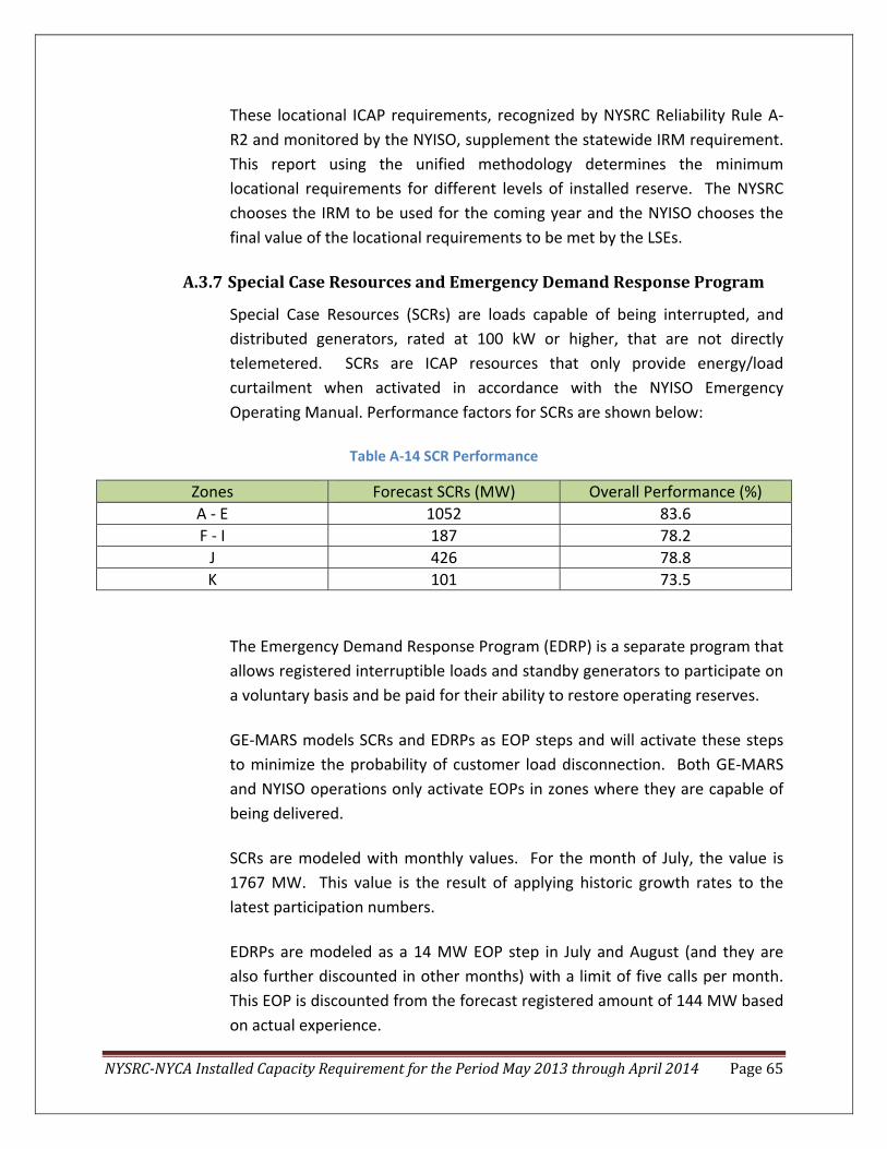
NYSRCNYCA Installed Capacity Requirement for the Period May 2013 through April 2014 Page 65
These locational ICAP requirements, recognized by NYSRC Reliability Rule A‐R2 and monitored by the NYISO, supplement the statewide IRM requirement. This report using the unified methodology determines the minimum locational requirements for different levels of installed reserve. The NYSRC chooses the IRM to be used for the coming year and the NYISO chooses the final value of the locational requirements to be met by the LSEs.
A.3.7 Special Case Resources and Emergency Demand Response Program
Special Case Resources (SCRs) are loads capable of being interrupted, and distributed generators, rated at 100 kW or higher, that are not directly telemetered. SCRs are ICAP resources that only provide energy/load curtailment when activated in accordance with the NYISO Emergency Operating Manual. Performance factors for SCRs are shown below:
Table A‐14 SCR Performance
Zones Forecast SCRs (MW) Overall Performance (%) A ‐ E 1052 83.6 F ‐ I 187 78.2 J 426 78.8 K 101 73.5
The Emergency Demand Response Program (EDRP) is a separate program that allows registered interruptible loads and standby generators to participate on a voluntary basis and be paid for their ability to restore operating reserves.
GE‐MARS models SCRs and EDRPs as EOP steps and will activate these steps to minimize the probability of customer load disconnection. Both GE‐MARS and NYISO operations only activate EOPs in zones where they are capable of being delivered.
SCRs are modeled with monthly values. For the month of July, the value is 1767 MW. This value is the result of applying historic growth rates to the latest participation numbers.
EDRPs are modeled as a 14 MW EOP step in July and August (and they are also further discounted in other months) with a limit of five calls per month. This EOP is discounted from the forecast registered amount of 144 MW based on actual experience.

NYSRCNYCA Installed Capacity Requirement for the Period May 2013 through April 2014 Page 66
A.4 MARS Data Scrub A.4.1 GE Data Scrub
General Electric was asked to review the input data for errors. GE has developed a program called “Data Scrub” which processes the input files and flags data that appears to be out of the ordinary. For example, it can identify a unit with a forced outage rate significantly higher than all the others in that size and type category. If something is found, the ISO reviews the data and either confirms that it is correct as is, or institutes a correction. The results of this data scrub are shown in Table A‐14.
Table A‐15 GE MARS Data Scrub
Item Description Disposition Model Change
Effect on IRM
1
Load data: The assumption matrix says NYCA’s load for 2013 should be 33,696 MW while the data has 33,927 MW modeled.
The NYCA peak load is now 33,278 MW, which is consistent with the October forecast, as specified by assumption matrix v5.3. NYC and LI’s peak loads are 11,532 MW and 5,553 MW, respectively.
No No
2
Non‐wind units: EnXco Solar is modeled as 11.35 MW, but the assumption matrix calls for 13.1 MW. FIT (Feed‐in‐tariff) is modeled as 14.73 MW, but the assumption matrix calls for 17 MW.
Solar units peak in August. Total solar equals 61.6 MW
No No
3
The assumption matrix called for 50 MW of scheduled maintenance during the summer period. The actual scheduled maintenance modeled during the peak week was 63.5 MW
The maintenance value is a nominal 50 MW. We select units that will approximate the 50 MW on summer maintenance.
No No
4 New Wind: Marble River was modeled with 215 MW during July, while the assumption matrix called for 216.3 MW.
Marble River – we used the Gold Book value of 215. Assumptions Matrix (AM) has been updated.
No No
5
Existing Wind: 1351 MW of wind was modeled during July, while the assumption matrix called for 1368.6 MW.
Not all the wind farms peak in July. Thus there is a nominal 18 MW difference in the MWs output. Our spreadsheet calculation accounts for the difference in the reserve margin calculation.
No No
6 Wind: 1566 MW of wind in total is being modeled during July, while the assumption matrix calls for 1585 MW.
Not all the wind farms peak in July. Thus there is a nominal 20 MW difference in the MWs output. Our spreadsheet calculation accounts for the difference in the reserve margin calculation.
No No
7 Existing Solar: 27.3 MW of solar is being modeled during July, while the assumption matrix calls for 31.5 MW.
Solar peaks in August, which shows the correct value of 31.5MW
No No

NYSRCNYCA Installed Capacity Requirement for the Period May 2013 through April 2014 Page 67
Item Description Disposition Model Change
Effect on IRM
8 New Solar: 26.08 MW of solar is being modeled during July, while the assumption matrix calls for 30.1 MW.
Solar peaks in August and shows the correct total value of 61.6MW
No No
9 Capacity Sales: We were unable to identify the capacity sales being modeled.
Resolved through discussions. No impact.
No No
10
Interface Limits: In the assumption matrix, West Central lists 1770 MW as a positive direction limit. We were unable to identify any way to make this rating apply based on the input data.
The model has been changed to allow this low load transfer limit. A subsequent run found no impact on the IRM.
Yes No
11
Interface Limits: In the assumption matrix, Volney East lists 4857 MW as the limit in the positive direction. This interface is modeled with a limit of 5675 MW in that direction.
Volney East is modeled as 5675 in the Model. The drawing has been updated.
No No
12
Interface Limits: In the assumption matrix, Zone D to Cedars is listed as a 1 MW limit leaving NYCA. This interface is modeled with a limit of 100 MW in that direction.
The rating has been corrected. A subsequent run found no impact on the IRM.
Yes No
13
Interface Limits: In the assumption matrix, Capital Hudson Valley is listed as a 3450 MW limit in the positive direction. This interface is modeled with a limit of 3475 MW in that direction.
Capital Hudson Valley is modeled as 3475 in the model. The drawing has been updated.
No No
14
Interface Limits: In the assumption matrix, Y49/Y50 is listed as a 530 MW limit in the negative direction. This interface is modeled with a limit of 344 MW in that direction.
The issue of this rating has been resolved. The limit remains unchanged at 530 MW.
No No
15 Interface Limits: The interface PJM to G + PJM to J is modeled, but is not described in the input assumptions.
The description is shown on Attachment E1 of the assumptions matrix.
No No
16
Special Case Resources: In the assumption matrix, the July 2013 SCR MWs should be 1437. In the model, the July SCRs are 1716 MW. (The June SCRs are 1437 MW, and the amounts by zone shown for June are consistent with the amounts shown in Attachment F).
July values should be 1437. Correction in database made.
Yes Yes
17
EDRP Resources: The assumption matrix states that both July and August will have a total of 14.4 MWs of EDRPs modeled. The August value in the model is actually 14.8 MW.
Forecast Registrations grow in August. The Assumptions Matrix has been changed to reflect this.
No No

NYSRCNYCA Installed Capacity Requirement for the Period May 2013 through April 2014 Page 68
Item Description Disposition Model Change
Effect on IRM
18
Other EOPs: Step 3, 5% manual voltage reduction, is listed as 66 MW in the input assumptions, but is modeled as 65 MW.
The Assumptions Matrix has been changed to reflect this.
No No
19
Other EOPs: Step 4, thirty minute reserve to zero, is listed as 600 MW in the input assumptions, but is modeled as 765 MW.
The AM has been updated to include the increase in reserves due to the Nine Mile 2 uprate. The 30 minute reserves were increased to 655 MW, while the 10 minute reserves were increased to 1310 MW.
Yes No
20
Other EOPs: Step 5, 5% remote voltage reduction, is listed as 486 MW in the input assumptions, but is modeled as 479 MW.
The Assumptions Matrix has been changed to reflect this.
No No
21
Interface Limits: In the assumption matrix, Zone D to Hydro Quebec is listed as a 1,500 MW limit entering NYCA. This interface is modeled with a limit of 410 MW in that direction.
The reduction in the limit to 410 MW reflects the 1090 MW of grandfathered contracts. The assumptions matrix shows the full emergency ratings of the ties.
No No
22
Interface Limits: In the assumption matrix, Hydro Quebec to Central MA is listed as a 1,400 MW limit flowing into New England. This interface is modeled with a summer limit of 900 MW and a winter limit of 1,400 MW flowing into New England.
The reduction in the limit to 900 MW reflects the 500 MW of firm contracts. The assumptions matrix shows the full emergency ratings of the ties.
No No
23
In the preliminary review, the contract definition for CON_CSC was highlighted as potentially being a source of errors in the future, due to its length in the MIF.
The mif was corrected to the 132 character limit with no impact.
Yes No
24
Since the preliminary review, the transition rate definitions for the DUNWOODI interface have been updated. These eight lines also exceed the maximum length of a MIF line in MARS, and some data is not being parsed by MARS for this interface
The mif was corrected to the 132 character limit with no impact.
Yes No
A.4.2 NYISO Data Scrub
The NYISO also performs a review of the MARS data independently from GE. Table A‐15 shows the results of this review.

NYSRCNYCA Installed Capacity Requirement for the Period May 2013 through April 2014 Page 69
Table A‐16 NYISO MARS Data Scrub
Item Description Disposition Model Change
Effect on IRM
1 Cedars tie has historically been 167 MW
Quebec has facilitated an increase of this tie to 190 MW
Yes No
2 Hillburn GT transition rates resulted in a incorrect EFOR
Rates corrected Yes No
3 Initial West Central interface ratings difference
Correction made without affecting results. Yes No
4 HTP line was not part of PJM output grouping
Model was updated to put HTP into this grouping
Yes No
A.4.3 Transmission Owner Data Scrub
In addition to the above reviews, two transmission owners scrub the data and assumptions from a masked database provided. Table A‐16 shows these results.
Table A‐17 Transmission Owner Data Scrub
Item Description Disposition Model Change
Effect on IRM
1 Why is HTP_PJME 1320?
When the potential resource is not needed by the NYISO, it can run to provide energy for PJM. In addition, the line would be available to deliver up to 660 MW of assistance to PJM from NY if NY has extra. The rating on the line into PJM accommodates this level. The model was developed several years ago by GE
No No
2 West Central (W_CENTRAL) should be 1770?
For times when the load is low, the initial limit of this dynamic rating is 1770 MW.
No No
3 Why is D_CEDARS derated 23 MW in May?
The rating should be 190 MW for the summer. The MARS results do not change because of this increase.
Yes No
5 Briefly describe why A_PJMW, C_PJMW, and C_PJMC are derated?
These interfaces are derated to accommodate the grandfathered (ETCNL) 1080 MW of which NYSEG owns the option. Note that their nominations are not made until the March following the IRM study completion.
No No
6 Why is UPNYSENY 1999? Ties may have higher ratings but load flow analysis never exceeds 2,000 MW
No No
7 Why is DSY49Y50 at 1999? Ties may have higher ratings but load flow analysis never exceeds 2,000 MW
No No

NYSRCNYCA Installed Capacity Requirement for the Period May 2013 through April 2014 Page 70
Item Description Disposition Model Change
Effect on IRM
8 Missing NEPOOL system bubble diagram in the assumption matrix.
We will include this in the IRM study report No No
9
The NYISO should provide bubble diagram for K2, K1A so QA can be done on the connections to other bubbles.
We will provide a diagram with confidential values redacted.
No No
10 Why is BEAUHA23 an EL1? This is a Quebec Unit. No No
11
For New England, ID‐360 (J. Cockwell unit 2) NYISO has a lower value than listed in the CELT report. Other than this unit, the rest of the NE units look fine.
Have resolved this with NE representative. No No

NYSRCNYCA Installed Capacity Requirement for the Period May 2013 through April 2014 Page 71
Appendix B
Details of Study Results

NYSRCNYCA Installed Capacity Requirement for the Period May 2013 through April 2014 Page 72

NYSRCNYCA Installed Capacity Requirement for the Period May 2013 through April 2014 Page 73
B. Details for Study Results B.1 Sensitivity Results
Table B‐1 summarizes the 2013 Capability Year IRM requirements under a range of assumption changes from those used for the base case. The base case utilized the computer simulation, reliability model, and assumptions described in Appendix A. The sensitivity cases determined the extent of how the base case required IRM would change for assumption modifications, either one at a time, or in combination. The methodology used to conduct the sensitivity cases was to start with the preliminary base case 17.2% IRM results then add or remove capacity from all zones in NYCA until the NYCA LOLE approached criteria. The values in Table B‐1 are the sensitivity results adjusted to the 17.1% final base.
Table B‐1 Sensitivity Case Results
Item Description IRM (%)
NYC (%) LI (%)
Transmission Sensitivities
2 No Internal NYCA Transmission Constraints (Free Flow System)
15.2 NA NA
This case represents the “Free‐Flow” NYCA case where internal transmission constraints are eliminated and measures the impact of transmission constraints on statewide IRM requirements. See the “Base Case – NYCA Transmission Constraints” section of the report.
12 Model 300 MW Wheel from HQ to NE through NYCA 17.5 86 101
A 300 MW wheel from Quebec to NE was modeled as an equivalent contract (derate Chateauquay tie by 300 MW and also derate ties from zones F and G to New England by an aggregate 300 MW).
Assistance from Outside World Modeling
1 NYCA Isolated 24.8 91 107
This case examines a scenario where the NYCA system is isolated and receives no emergency assistance from neighboring control areas (New England, Ontario, Quebec, and PJM). UDRs are allowed. See the “Base Case Results – Interconnection Support during Emergencies” section of the report.

NYSRCNYCA Installed Capacity Requirement for the Period May 2013 through April 2014 Page 74
6 Higher Outside World Margins 10.9 81 96
Increases each external Control Area’s Reserve Margin by lowering their load by 10%. Examines the NYCA IRM under the conditions where external Control Area’s have additional capacity which could help NYCA in emergencies.
7 Lower Outside World Margins 23.2 90 106
Decreases each external Control Area’s Reserve Margin by increasing their load by 10%. Examines the NYCA IRM under conditions where external Control Areas have less capacity available to help NYCA in emergencies.
Generation Sensitivities
8 Increase EFORs from Base Case 18.6 87 102
This shows the impact of the NYCA units having higher EFORds than the base case. Higher EFORds indicate less capacity available to meet the criterion. The case is accomplished by increasing thermal unit EFORs by 1.0 percentage point.
9 Decrease EFORs from Base Case 16.4 85 100
This shows the impact of the NYCA units having lower EFORs than the base case. Lower EFORds indicate more capacity available to meet the criterion. The case is accomplished by reducing thermal unit EFORs by 1.0 percentage point (Units already better than 1.0% EFOR were left alone).
11 Retirement of Indian Point 2 and 3 22.1 93 110
Removes the Indian Point plant and returns capacity (as per the sensitivity procedure) to all NY zones. This case did not evaluate the impact of the retirement on transfer capability and kept all interface ratings unchanged.
4 Remove all wind generation 12.7 85 101
Freeze J & K at base levels and adjust capacity in the upstate zones. This shows the impact that the wind generation has on the IRM requirement.

NYSRCNYCA Installed Capacity Requirement for the Period May 2013 through April 2014 Page 75
15 Add units that were retired after the Base Case was run. 16.7 85 101
Show impact of additional retirements. Capacity was added to zones A‐I.
Load Sensitivities
3 No Load Forecast Uncertainty 7.8 79 94
This scenario represents “perfect vision” for 2013 peak loads, assuming that the forecast peak loads for NYCA have a 100% probability of occurring. The results of this evaluation help to quantify the effects of weather on IRM requirements.
10 Run study with 2007 load shape 14.4 80 96
Using the 2007 shape, which is more typical than the 2002 load shape. (results are from knee of curve)
Emergency Operating Procedures
5 No SCRs or EDRPs 16.6 85 103
Shows the impact of SCRs and EDRPs on IRM.
13 Limit SCRs 5 calls per month. 20.2 88 104
Shows the impact on the IRM of limited help from SCRs.
Environmental Initiative Effecting IRM
14 Coal Unit Retirements (as in the RNA) 17.8 85 101
Retire all coal units and replace with capacity in zones A‐I. Shows possible future year impact due to economic and environmental initiatives.

NYSRCNYCA Installed Capacity Requirement for the Period May 2013 through April 2014 Page 76
B.2 Environmental Impacts Various environmental initiatives driven by the State and/or Federal regulators are either in place or are pending that will affect the operation of the existing fleet. The United States Environmental Protection Agency (USEPA) has promulgated several regulations that will affect most of the thermal fleet of generators in NYCA. Similarly, the New York State Department of Environmental Conservation (NYSDEC) has undertaken the development of several regulations that will apply to most of the thermal fleet in New York.
The control technology retrofit requirements of five environmental initiatives are sufficiently broad in application that certain generator owners may need to address the retirement versus retrofit question. These environmental initiatives are: (i) NYSDEC’s Reasonably Available Control Technology for Oxides of Nitrogen (NOx RACT); (ii) Best Available Retrofit Technology (BART) to address regional haze; (iii) Best Technology Available (BTA) for cooling water intake structures; (iv) the USEPA’s Mercury and Air Toxics Standards (MATS); and (v) either the Cross State Air Pollution Rule (CSAPR) or its predecessor the Clean Air Interstate Rule (CAIR) addressing interstate transport of criteria air pollutants.
The NYISO has determined that as many as 33,963 MW in the existing fleet will have some level of exposure to the new regulations as detailed in the 2012 Reliability Needs Assessment (RNA) and further discussed in this review. The magnitude of the combined investments required to comply with the five initiatives could lead to multiple unplanned plant retirements.
B.2.1 Reasonably Available Control Technology for Oxides of Nitrogen (NOx RACT)
NYS DEC finalized new regulations for the control of emissions of nitrogen oxides (NOx) from fossil fueled power plants (Part 227‐2). The regulations establish presumptive emission limits for each type of fossil fueled generator and each fuel used in an electric generator in New York that has a capacity greater than 25 MW. Compliance options include averaging emissions with lower emitting units, fuel switching, and installing emission reduction equipment such as low NOx burners or combustors, selective catalytic reduction units, or retirement. Generators were required to file permit applications and a RACT analysis with NYSDEC by January 1, 2012. Compliance with approved plans is required by July 1, 2014.

NYSRCNYCA Installed Capacity Requirement for the Period May 2013 through April 2014 Page 77
(1) NOx RACT Impact Assessment
NOx RACT compliance plans and permit applications were required to be filed by the end of 2011. Reviewing the plans that are public, approximately 25,800 MW of capacity are subject to this rule, of which approximately 6,000 MW of capacity are involved in emission reduction projects. Some of these projects are underway, and the balance should be accomplished prior to the July 2014 compliance date.
B.2.2 Best Available Retrofit Technology (BART)
The NYSDEC has promulgated Part 249, Requirements for the Applicability, Analysis, and Installation of Best Available Retrofit Technology (BART) Controls. The regulation applies to fossil fueled electric generating units built between August 7, 1962 and August 7, 1977 and is necessary for New York State to comply with provisions of the federal Clean Air Act that are designed to improve visibility in National Parks. The regulation requires an analysis to determine the impact of an affected unit’s emissions on visibility in national parks. If the impacts are greater than a prescribed minimum, then emission reductions must be made at the affected unit. Emissions controls for sulfur dioxide (SO2), nitrogen oxides (NOx) and particulate matter (PM) may be necessary. Each affected generator was required to submit an analysis to the NYSDEC in October 2010. The compliance deadline is January 2014.
(1) BART Impact Assessment
The results of the visibility analysis are used to determine the emission reductions that may be necessary for SO2, NOx, and PM. USEPA has established a presumptive set of emission limits for 8,600 MW of affected units. The majority of these units are large oil fired units that have gas as an alternate fuel. Many of these units do not have state of the art emission control systems.
The NOx control measures for BART generally were consistent with the results of the NOx RACT study. The NYSDEC has established a reasonableness test of $5,500/ton reduced. Capital expenditures for this program would be of the same order of magnitude as the NOx RACT program.
The NYSDEC has reviewed these plans and is in the process of issuing amended Title V stationary source permits. USEPA announced final approval of compliance plans for most of the generators, while several of

NYSRCNYCA Installed Capacity Requirement for the Period May 2013 through April 2014 Page 78
the proposed plans will need to be revised based on alternative limits that EPA has proposed as being more appropriate.
In order to gauge the impact of these regulations, historic emissions and inventories of installed emission control equipment have been reviewed to estimate the level of additional emission reductions required. Most of the affected capacity can comply with the emission limits with optimum operation of existing environmental control equipment and/or fuel switching. Several small units have chosen to retire, which represents a capacity loss of less than 50 MW. Other plants will achieve the required emission reductions through the use of cleaner fuels, while others are undertaking retrofit projects. Approximately 1,800 MW of capacity may be required to undertake a major emissions reduction project or switch to cleaner fuels. Five units, Northport 1, 2, 3, & 4 and Danskammer 4, may be required to retrofit environmental control technology.
B.2.3 Mercury Air Toxics Standard (MATS)
The USEPA announced the final MATs rule in December, 2011. The proposed rule previously had been known as the Maximum Achievable Control Technology (MACT) Rule for Hazardous Air Pollutants (HAPS). The rule establishes limits for acid gases, Hydrogen Chloride (HCl), Hydrogen Fluoride (HF), Mercury (Hg), and Particulate Matter (PM). Alternative limits were also established. MATS limits will apply to coal and/or oil‐fired generators. The compliance date is March 2015. The NYSDEC may provide an additional year to comply if necessary. Further, reliability critical units can qualify for another year to achieve compliance if the additional year is necessary to complete the retrofitting of emissions control technology or to allow for the alternate reliability improvement project to be completed.
In addition, the NYSDEC has promulgated Part 246: Mercury Reduction Program for Coal‐Fired Electric Utility Steam Generating Units, which establishes emission limitations that are currently in effect in New York to reduce mercury emissions. Phase II of this regulation requires additional reductions for coal fired boilers in 2015. The Phase II emission limitations are more stringent than the USEPA MATS limits.
(1) MATS Impact Assessment
The USEPA announced the final rule for MATS for fossil fired electric generators in December. The regulations apply to coal and oil fueled

NYSRCNYCA Installed Capacity Requirement for the Period May 2013 through April 2014 Page 79
electric generators greater than 25 MW. Units with 10,300 MW of capacity in New York will be affected by this regulation.
The USEPA established a subcategory for limited use oil‐fired generators. Units that maintain a capacity factor on oil that is less than 8% will be more lightly regulated. No oil‐fired EGUs exceeded the 8% Capacity Factor while firing oil in 2009‐2011. Although these units will remain subject to MATS, mandatory significant emission control retrofit projects are not expected at these units.
The coal fired generators subject to MATS are also subject to the NYSDEC Part 246 Phase 2 regulations for limitations on mercury emissions. These regulations are more stringent than the USEPA MATS regulations. The review of potential impacts for coal units focused on emissions of PM and acid gases in the form of HCl. Alternative emission limits are also provided for Non‐Hg Metals and SO2. Historic emissions and inventories of installed emission control equipment have been reviewed to estimate the level of additional emission reductions required. With optimum operation of existing environmental control equipment and/or fuel switching, most of the affected coal capacity can comply with the emission limits.
B.2.4 Best Technology Available (BTA)
USEPA has proposed Section 316 b rules that set standards for the design and operation of open cycle cooling systems. This rule will be implemented by NYSDEC, which has finalized a policy for the implementation of this rule known as “Best Technology Available (BTA) for Cooling Water Intake Structures”. The policy applies to plants with design intake capacity greater than 20 million gallons/day and prescribes reductions in fish mortality. The proposed policy establishes performance goals for new and existing cooling water intake structures. The performance goals call for the use of wet, closed‐cycle cooling systems at existing generating facilities. Limited relief is available for sites that cannot physically accommodate cooling towers, generators with historical capacity factors below 15%, and where the expense of a closed cooling water system is “wholly disproportionate” compared to the environmental benefits to be gained. The policy is applied at the time that a plant’s State Pollution Discharge Elimination System permit is renewed, which is theoretically every five years.

NYSRCNYCA Installed Capacity Requirement for the Period May 2013 through April 2014 Page 80
(1) BTA Impact Assessment
The NYSDEC has made twelve BTA determinations of which two determinations required the use of closed cycle cooling systems. Although the number of impacted MWs is unknown, for study purposes the NYISO shows a range from 4,000 MW to 7,000 MW. This program will require capital investments that are one to two orders of magnitude greater than the cumulative costs for the other environmental initiatives examined. Consequently, the BTA program has the greatest potential to lead to previously unplanned retirements.
B.2.5 Cross State Air Pollution Rule (CSAPR)12
The USEPA finalized the CASPR rule in December 2011. The rule is designed to reduce emissions of SO2, Annual NOx and Ozone Season NOx from fossil fueled power plants in 28 central and eastern states. The regulation is implemented through the use of emission allowances and limited emissions trading programs. The regulation establishes emission budgets for each affected state. The emission budget is then divided on a pro‐rata basis determined by historic heat input for existing facilities. There are ‘set asides’ to provide allowances to new fossil generators. The use of emission allowances is expected to increase offering prices for generation from affected facilities. The final rule was placed under a stay by a federal District Court. But for the action of the courts, the rule would be in effect currently with another reduction in the SO2 cap scheduled for 2014. While this rule is currently the subject of litigation, it is included it in our analysis because additional cross state emissions controls are likely to be implemented in some form.
CSAPR is USEPA’s revision of the Clean Air Interstate Rule (CAIR) which was vacated by the U.S. Supreme Court. In doing so, the Court ordered that CAIR remain in effect until such time as replacement rule is implemented. In December 2011, when the District Court stayed the CSAPR rule, it ordered that CAIR be reinstated. CAIR as promulgated requires significant reductions
12 A three‐judge panel of the United States Court of Appeals for the District of Columbia Circuit vacated, in an order issued August 21, 2012, the final Transport Rule (CSAPR), and the Transport Rule Federal Implementation Plans. The Court remanded the proceeding to the Environmental Protection Agency and ordered it to continue to administer CAIR pending a valid replacement.

NYSRCNYCA Installed Capacity Requirement for the Period May 2013 through April 2014 Page 81
in allowable emissions scheduled for 2015. Because the federal Clean Air Act provides for reductions in interstate air pollutant transport, it is reasonable to assume that a national interstate program will be in effect for limiting emissions of SO2 and NOx via a cap and trade program in the early part of the ten‐year planning horizon evaluated in the RNA. Therefore, the CSAPR rule will be used to evaluate the potential impacts of that program.
(1) CSAPR Impact Assessment
The CSAPR rule applies to most of the fossil fueled fleet with nameplate capacity greater than 25 MW. The rule will require the use of allowances in numbers equivalent to actual emissions for SO2, Annual NOx, and for Ozone Season NOx. The budget for each of the states in the program has been established by the USEPA through the use of long range transport models to identify sources and sinks for impact of emissions on areas in other states. The budget of allowances for each of the three categories is distributed on a pro‐rata basis developed on historic heat input at affected units. A small set‐aside is established for new units and recently retired units to continue to receive allowances for a limited time period. The rule calls for a two phase reduction of SO2, while the limits for Annual NOx and Ozone Season NOx are fixed. The program limits the amount of allowances that can be obtained through trading with generator owners in other states. The total of the budget plus traded allowances is known as the “Assurance Level.” Should a state’s emissions exceed the Assurance Level, two additional allowances would need to be surrendered for the excess emissions. This penalty would be prorated across all emitters.
Historic emissions and inventories of installed emission control equipment have been reviewed to estimate the level of additional emission reductions required. With optimum operation of existing environmental control equipment and/or fuel switching, New York State should be able to operate within the Assurance Level.
B.2.6 Summary of Environmental Programs
The table below summarizes the new environmental requirements that were known to come into effect in the near term and the amounts of capacity that would be affected by each of these regulations. In addition, the quantities of capacity and number of units that have announced or are expected to undertake environmental control projects to achieve compliance are also

NYSRCNYCA Installed Capacity Requirement for the Period May 2013 through April 2014 Page 82
tabulated. Of the environmental programs examined, only the BTA program could have effective compliance dates in 2013. Two small coal burning units have announced retirements to comply with BART. While environmental compliance options and related costs are a consideration in planning for a going concern in the post 2013 timeframe, these environmental regulations will not by themselves require retirements in 2013.
Table B‐2 Summary of Environmental Programs
Program Status Compliance Deadline Approximate Capacity affected
Potential Retrofits
NOx RACT In Effect July 1, 2014 28,700 MW (294 Units)
6,000 MW (23 Units)
BART In Effect January 1, 2014 8,600 MW (19 Units)
1,800 MW (5 Units)
MATS In Effect April 16, 2015,6,or 7 11,000 MW (32 Units)
400 MW (2 Units)
BTA In Effect Upon Permit Renewal 17,400 MW (42 Units)
4,400 to 7,300 MW
CSAPR Implementation is
stayed while the rule is in litigation
January 1, 2012 and January 1, 2014 26,800 MW (162 Units)
2,400 MW (11 Units)
B.3 Frequency of Implementing Emergency Operating Procedures In all cases, it was assumed that the EOPs are implemented as required to meet the 0.1 days/year criterion. For the base case, the study shows that approximately 9.0 remote voltage reductions per year would be implemented to meet the once in 10 years disconnection criterion. The expected frequency for each of the EOPs for the base case is provided in Table B‐3.

NYSRCNYCA Installed Capacity Requirement for the Period May 2013 through April 2014 Page 83
Table B‐3 Implementation of EOP steps
Step EOP Expected Implementation
(Days/Year) 1 Require SCRs 17.8 2 Require EDRPs 10.1 3 5% manual voltage reduction 9.3 4 30 minute reserve to zero 9.2 5 5% remote control voltage reduction 9.0 6 Voluntary load curtailment 5.5 7 Public appeals 4.1 8 Emergency purchases 3.7 9 10 minute reserve to zero 3.5 10 Customer disconnections 0.1

NYSRCNYCA Installed Capacity Requirement for the Period May 2013 through April 2014 Page 84

NYSRCNYCA Installed Capacity Requirement for the Period May 2013 through April 2014 Page 85
Appendix C
ICAP to UCAP Translations

NYSRCNYCA Installed Capacity Requirement for the Period May 2013 through April 2014 Page 86

NYSRCNYCA Installed Capacity Requirement for the Period May 2013 through April 2014 Page 87
C. ICAP to UCAP Translation The NYISO administers the capacity requirements to all loads in the NYCA. In 2002, the NYISO adopted the Unforced Capacity (UCAP) methodology for determining system requirements, unit ratings and market settlements. The UCAP methodology uses individual generating unit data for output and availability to determine an expected level of resources that can be considered for system planning, operation and marketing purposes. EFORd is developed from this process for each generating unit and applied to the units Dependable Maximum Net Capability (DMNC) test value to determine the resulting level of UCAP.
Individual unit EFORd factors are taken in aggregate on both a Statewide and Locational basis and used to effectively “translate” the IRM and LCRs previously determined in the GE‐MARS Analysis in terms of ICAP, into an equivalent UCAP basis.
Table C‐1 summarizes historical values (since 2000) for NYCA capacity parameters including Base Case IRMs, approved IRMs, UCAP requirements, and NYISO Approved LCRs (for NYC and LI).
Table C‐1 Historical NYCA Capacity Parameters
Capability Year Base Case IRM (%)
EC‐Approved IRM (%)
NYCA Equivalent UCAP
Requirement (%)
NYISO ‐ Approved NYC LCR (%)
NYISO – Approved LI LCR (%)
2000 15.5 18.0 80 107 2001 17.1 18.0 80 98 2002 18.0 18.0 80 93 2003 17.5 18.0 80 95 2004 17.1 18.0 11.9 80 99 2005 17.6 18.0 12.0 80 99 2006 18.0 18.0 11.6 80 99 2007 16.0 16.5 11.3 80 99 2008 15.0 15.0 8.4 80 94 2009 16.2 16.5 7.2 80 97.5 2010 17.9 18.0 6.1 80 104.5 2011 15.5 15.5 8.2 81 101.5 2012 16.1 16.0 5.4 83 99

NYSRCNYCA Installed Capacity Requirement for the Period May 2013 through April 2014 Page 88
C.1 NYCA and NYC and LI Locational Translations In the “Installed Capacity” section of the NYISO Web site, the NYISO Staff regularly posts ICAP and UCAP calculations for both the summer and winter Capability Periods. This publicly available information can be found on the NYISO web site.13
Information has been compiled by the NYISO on this site since 2006 and includes complete information through 2011. This information is provided for Locational Areas and for the Transmission District Loads.
The Locational Areas include NYC, LI and the entire NYCA. Exhibits C‐1(a) through C‐1(c) summarizes translation of ICAP requirements to UCAP requirements for these Locational Areas. The charts and tables included in these exhibits utilize data from the 2006‐2011 capability periods (and limited to “summer” only, for purposes of simplicity).
Importantly, this data reflects the interaction and relationships between the capacity parameters used this study, including Forecast Peak Load, ICAP Requirements, Derating Factors, UCAP Requirements, IRM and LCRs. Since these parameters are so inextricably linked to each other, the graphical representation also helps one more easily visualize the annual changes in capacity requirements.
Several interesting observations can be made from these results. For example, in the NYCA chart (Figure C‐2), the IRMs generally stayed the same or increased from 2007 on while the UCAP MWs fell from 37,228 MW to 35,076 MW.
These charts also use approved LCR which depicts the dynamics of the LCRs upon the NYC and LI locational areas. For example, in the New York City chart (Figure C‐3), the ICAP and UCAP values remained relatively constant despite a rapid increase in the LCRs levels from 80% to 83%.
For Long Island (Figure C‐4), LCRs produced ICAP and UCAP curves of similar shape; it is easy to see how LCR influences these parameters. Over the period shown, the LCRs for LI both increased and decreased with the ICAP and UCAP requirements generally following suit.
13 http://icap.nyiso.com/ucap/public/ldf_view_icap_calc_selection.do

NYSRCNYCA Installed Capacity Requirement for the Period May 2013 through April 2014 Page 89
C.1.1 New York Control Area ICAP to UCAP Translation
Table C‐2 NYCA ICAP to UCAP Translation
114
115
116
117
118
119
120
32,000
33,000
34,000
35,000
36,000
37,000
38,000
39,000
40,000
2006 2007 2008 2009 2010 2011 2012
Statewide % ICAP Requirement
Megawatts (M
W)
NYCA TotalCapacity Parameters: Forecast Peak Load, ICAP, UCAP, IRM ‐ Summer 2006‐2012
FC Peak Load Required ICAP Required UCAP % ICAP Required
YearForecast Peak Load (MW)
ICAP Requirement
(%)
Derate Factor (%)
ICAP Requirement
(MW)
UCAP Requirement
(MW)
Effective UCAP (%)
2006 33,295 118.0 0.0543 39,288 37,154 111.62007 33,447 116.5 0.0446 38,966 37,228 111.32008 33,809 115.0 0.0578 38,880 36,633 108.42009 33,930 116.5 0.0801 39,529 36,362 107.22010 33,025 118.0 0.1007 38,970 35,045 106.12011 32,714 115.5 0.0820 37,920 34,987 106.02012 33,295 116.0 0.0918 38,622 35,076 105.4

NYSRCNYCA Installed Capacity Requirement for the Period May 2013 through April 2014 Page 90
C.1.2 New York City ICAP to UCAP Translation
Table C‐3 New York City ICAP to UCAP Translation
YearForecast Peak Load (MW)
ICAP Requirement
(%)
Derate Factor (%)
ICAP Requirement
(MW)
UCAP Requirement
(MW)
Effective UCAP (%)
2006 11,628 80.0 0.0542 9,302 8,798 75.72007 11,780 80.0 0.0388 9,424 9,058 76.92008 11,964 80.0 0.0690 9,571 8,911 74.52009 12,050 80.0 0.0814 9,640 8,855 73.52010 11,725 80.0 0.1113 9,380 8,336 71.12011 11,514 81.0 0.0530 9,326 8,832 76.72012 11,500 83.0 0.0679 9,545 8,897 77.4
78
79
80
81
82
83
84
8,000
8,500
9,000
9,500
10,000
10,500
11,000
11,500
12,000
12,500
2006 2007 2008 2009 2010 2011 2012
Locational Capacity Requirement (LCR) %
Megawatts (M
W)
New York City (NYC) ‐ Zone JCapacity Parameters: Forecast Peak Load, ICAP, UCAP, LCRs ‐ Summer 2006‐2012
Peak Load Forecast Required ICAP Required UCAP LCR %
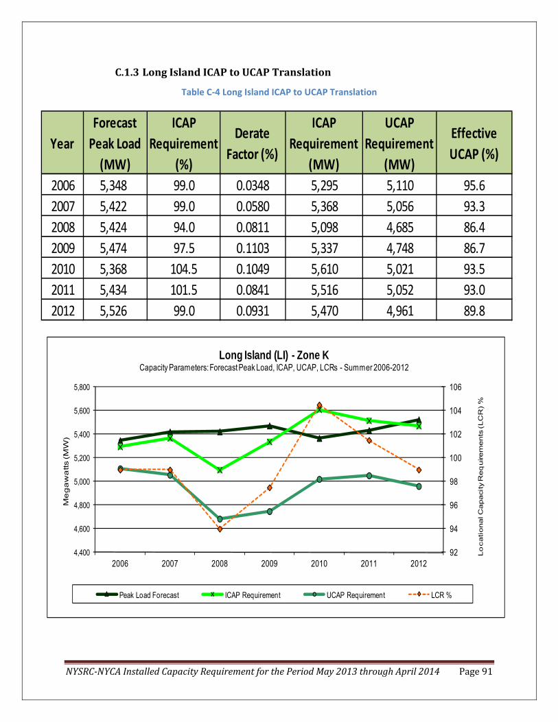
NYSRCNYCA Installed Capacity Requirement for the Period May 2013 through April 2014 Page 91
C.1.3 Long Island ICAP to UCAP Translation
Table C‐4 Long Island ICAP to UCAP Translation
YearForecast Peak Load (MW)
ICAP Requirement
(%)
Derate Factor (%)
ICAP Requirement
(MW)
UCAP Requirement
(MW)
Effective UCAP (%)
2006 5,348 99.0 0.0348 5,295 5,110 95.62007 5,422 99.0 0.0580 5,368 5,056 93.32008 5,424 94.0 0.0811 5,098 4,685 86.42009 5,474 97.5 0.1103 5,337 4,748 86.72010 5,368 104.5 0.1049 5,610 5,021 93.52011 5,434 101.5 0.0841 5,516 5,052 93.02012 5,526 99.0 0.0931 5,470 4,961 89.8
92
94
96
98
100
102
104
106
4,400
4,600
4,800
5,000
5,200
5,400
5,600
5,800
2006 2007 2008 2009 2010 2011 2012
Lo
cational C
apaci
ty R
eq
uire
ments
(LC
R) %
Me
ga
wa
tts (M
W)
Long Island (LI) - Zone KCapacity Parameters: Forecast Peak Load, ICAP, UCAP, LCRs - Summer 2006-2012
Peak Load Forecast ICAP Requirement UCAP Requirement LCR %

NYSRCNYCA Installed Capacity Requirement for the Period May 2013 through April 2014 Page 92
C.2 Transmission Districts ICAP to UCAP Translation C.2.1 Central Hudson Gas & Electric
Table C‐5 Central Hudson Gas & Electric ICAP to UCAP Translation
114%
115%
116%
117%
118%
119%
120%
1,100
1,150
1,200
1,250
1,300
1,350
1,400
1,450
2006 2007 2008 2009 2010 2011 2012
Sta
tew
ide %
ICA
P R
eq
uir
em
ent
Me
ga
wa
tts (M
W)
Central Hudson Gas & Electric (CHGE)Capacity Parameters: Forecast Peak Load, ICAP, UCAP, IRM - Summer 2006-2012
Forecast Peak Load Required ICAP Required UCAP % ICAP Requirement
Year Forecast
Peak Load (MW)
ICAP Requirement
(MW)
UCAP Requirement
(MW)
% ICAP of Forecast
Peak
% UCAP of Forecast Peak
2006 1163 1372 1297 118.0 111.6 2007 1205 1404 1341 116.5 111.3 2008 1214 1396 1316 115.0 108.4 2009 1196 1394 1282 116.5 107.2 2010 1172 1383 1244 118.0 106.1 2011 1177 1359 1248 115.5 106.0 2012 1133 1315 1194 115.5 106.0

NYSRCNYCA Installed Capacity Requirement for the Period May 2013 through April 2014 Page 93
C.2.2 Consolidated Edison (Con Ed)
Table C‐6 Con Ed ICAP to UCAP Translation
114%
115%
116%
117%
118%
119%
120%
12,500
13,000
13,500
14,000
14,500
15,000
15,500
16,000
16,500
17,000
2006 2007 2008 2009 2010 2011 2012
Stat
ewid
e %
ICAP
Req
uire
men
t
Meg
awat
ts (M
W)
Consolidated Edison (Con Ed)Capacity Parameters: Forecast Peak Load, ICAP, UCAP, IRM - Summer 2006-2012
Forecast Peak Load Required ICAP Required UCAP % ICAP Required
Year Forecast
Peak Load (MW)
ICAP Requirement
(MW)
UCAP Requirement
(MW)
% ICAP of Forecast
Peak
% UCAP of Forecast Peak
2006 13,400 15,812 14,953 118.0 111.6 2007 13,634 15,883 15,175 116.5 111.3 2008 13,911 15,998 15,073 115.0 108.4 2009 14,043 16,360 15,050 116.5 107.2 2010 13,655 16,113 14,490 118.0 106.1 2011 13,451 15,535 14,261 115.5 106.0 2012 13,431 15,579 14,149 116.0% 105.4%

NYSRCNYCA Installed Capacity Requirement for the Period May 2013 through April 2014 Page 94
C.2.3 Long Island Power Authority (LIPA)
Table C‐7 LIPA ICAP to UCAP Translation
114%
115%
116%
117%
118%
119%
120%
5,000
5,200
5,400
5,600
5,800
6,000
6,200
6,400
6,600
2006 2007 2008 2009 2010 2011 2012
Sta
tew
ide %
ICA
P R
eq
uir
em
ent
Me
ga
wa
tts (M
W)
Long Island Power Authority (LIPA)Capacity Parameters: Forecast Peak Load, ICAP, UCAP, IRM - Summer 2006-2012
FC Peak Load Req. ICAP Req. UCAP % Required ICAP
Year Forecast
Peak Load (MW)
ICAP Requirement
(MW)
UCAP Requirement
(MW)
% ICAP of Forecast
Peak
% UCAP of Forecast Peak
2006 5406 6379 6033 118.0 111.6 2007 5322 6200 5923 116.5 111.3 2008 5359 6163 5807 115.0 108.4 2009 5432 6328 5821 116.5 107.2 2010 5286 6238 5609 118.0 106.1 2011 5404 6242 5370 115.5 106.0 2012 5508 6390 5803 116.0 105.4

NYSRCNYCA Installed Capacity Requirement for the Period May 2013 through April 2014 Page 95
C.2.4 National Grid (NGRID)
Table C‐8 NGRID ICAP to UCAP Translation
114%
115%
116%
117%
118%
119%
120%
6,000
6,500
7,000
7,500
8,000
8,500
2006 2007 2008 2009 2010 2011 2012
Sta
tew
ide
% IC
AP
Req
uire
men
t
Me
ga
wa
tts (M
W)
National Grid (NGrid)Capacity Parameters: Forecast Peak Load, ICAP, UCAP, IRM - Summer 2006-2012
FC Peak Load Req. ICAP Req. UCAP % Required ICAP
Year Forecast
Peak Load (MW)
ICAP Requirement
(MW)
UCAP Requirement
(MW)
% ICAP of Forecast
Peak
% UCAP of Forecast Peak
2006 7052 8321 7869 118.0 111.6 2007 6719 7827 7478 116.5 111.3 2008 6763 7777 7327 115.0 108.4 2009 6728 7839 7211 116.5 107.2 2010 6732 7944 7144 118.0 106.1 2011 6575 7594 6971 115.5 106.0 2012 6749 7829 7110 116.0 105.4

NYSRCNYCA Installed Capacity Requirement for the Period May 2013 through April 2014 Page 96
C.2.5 New York Power Authority (NYPA)
Table C‐9 NYPA ICAP to UCAP Translation
114%
115%
116%
117%
118%
119%
120%
300
350
400
450
500
550
600
650
700
750
2006 2007 2008 2009 2010 2011 2012
Sta
tew
ide %
ICA
P R
eq
uir
em
ent
Meg
aw
atts (M
W)
New York Power Authority (NYPA)Capacity Parameters: Forecast Peak Load, ICAP, UCAP, IRM - Summer 2006-2012
Forecast Peak Load Required ICAP Required UCAP % ICAP Required
Year Forecast
Peak Load (MW)
ICAP Requirement
(MW)
UCAP Requirement
(MW)
% ICAP of Forecast
Peak
% UCAP of Forecast Peak
2006 584 689 652 118.0 111.6 2007 588 685 655 116.5 111.3 2008 579 666 628 115.0 108.4 2009 587 684 629 116.5 107.2 2010 318 375 337 118.0 106.1 2011 320 369 339 115.5 106.0 2012 576 668 607 116.0 105.3

NYSRCNYCA Installed Capacity Requirement for the Period May 2013 through April 2014 Page 97
C.2.6 New York State Electric & Gas (NYSEG)
Table C‐10 NYSEG ICAP to UCAP Translation
114%
115%
116%
117%
118%
119%
120%
2,700
2,900
3,100
3,300
3,500
3,700
3,900
2006 2007 2008 2009 2010 2011 2012S
tate
wid
e %
ICA
P R
eq
uir
em
ent
Me
ga
wa
tts (M
W)
New York State Electric & Gas (NYSEG)Capacity Parameters: Forecast Peak Load, ICAP, UCAP, IRM - Summer 2006-2012
Forecast Peak Load Required ICAP Required UCAP % ICAP Required
Year Forecast
Peak Load (MW)
ICAP Requirement
(MW)
UCAP Requirement
(MW)
% ICAP of Forecast
Peak
% UCAP of Forecast Peak
2006 2932 3459 3271 118.0 111.6 2007 3217 3748 3581 116.5 111.3 2008 3141 3612 3404 115.0 108.4 2009 3112 3625 3335 116.5 107.2 2010 3075 3629 3263 118.0 106.1 2011 3037 3508 3220 115.5 106.0 2012 3127 3627 3294 116.0 105.4

NYSRCNYCA Installed Capacity Requirement for the Period May 2013 through April 2014 Page 98
C.2.7 Orange & Rockland (O & R)
Table C‐11 O & R ICAP to UCAP Translation
114%
115%
116%
117%
118%
119%
120%
1,050
1,100
1,150
1,200
1,250
1,300
1,350
1,400
1,450
2006 2007 2008 2009 2010 2011 2012
Sta
tew
ide %
ICA
P R
eq
uir
em
ent
Meg
aw
atts (M
W)
Orange & Rockland (O&R)Capacity Parameters: Forecast Peak Load, ICAP, UCAP, IRM - Summer 2006-2012
Forecast Peak Load Required ICAP Required UCAP % ICAP Required
Year Forecast
Peak Load (MW)
ICAP Requirement
(MW)
UCAP Requirement
(MW)
% ICAP of Forecast
Peak
% UCAP of Forecast Peak
2006 1130 1333 1261 118.0 111.6 2007 1132 1318 1259 116.5 111.3 2008 1192 1371 1292 115.0 108.4 2009 1180 1374 1264 116.5 107.2 2010 1157 1366 1228 118.0 106.1 2011 1173 1355 1243 115.5 106.0 2012 1158 1344 1220 116.0 105.4

NYSRCNYCA Installed Capacity Requirement for the Period May 2013 through April 2014 Page 99
C.2.8 Rochester Gas & Electric (RGE)
Table C‐12 RGE ICAP to UCAP Translation
114%
115%
116%
117%
118%
119%
120%
1,500
1,550
1,600
1,650
1,700
1,750
1,800
1,850
1,900
1,950
2,000
2006 2007 2008 2009 2010 2011 2012
Sta
tew
ide %
ICA
P R
eq
uir
em
ent
Meg
aw
atts (M
W)
Rochester Gas & Electric (RGE)Capacity Parameters: Forecast Peak Load, ICAP, UCAP, IRM - Summer 2006-2012
Forecast Peak Load Required ICAP Required UCAP % ICAP Required
Year Forecast
Peak Load (MW)
ICAP Requirement
(MW)
UCAP Requirement
(MW)
% ICAP of Forecast
Peak
% UCAP of Forecast Peak
2006 1629 1922 1817 118.0 111.6 2007 1632 1901 1816 116.5 111.3 2008 1649 1897 1787 115.0 108.4 2009 1652 1925 1771 116.5 107.2 2010 1630 1923 1729 118.0 106.1 2011 1576 1821 1671 115.5 106.0 2012 1612 1870 1699 116.0 105.4

NYSRCNYCA Installed Capacity Requirement for the Period May 2013 through April 2014 Page 100
C.3 Wind Resource Impact on the NYCA IRM and UCAP Markets Wind generation is generally classified as an “intermittent" or "variable generation" resource with a limited ability to be dispatched. The effective capacity of wind generation can be quantified and modeled using the GE‐MARS program similar to conventional fossil‐fired power plants. There are various modeling techniques to model wind generation in GE‐MARS; the method that ICS has adopted uses historical hourly wind farm generation outputs. This data can be scaled to the nameplate capacity and assigned geographically to new and existing wind generation units.
Several new wind generation resources have been added to the NYCA. However due to the intermittent nature of the wind, these resources cannot always be counted on to be available when the NYCA needs them.
For a wind farm or turbine, the nameplate capacity is the ICAP while the effective capacity is equal to the UCAP value. Seasonal variability and geographic location are factors that also affect wind resource availability. The effective capacity of wind generation can be either calculated statistically directly from historical hourly wind generation outputs, and/or by using the following information:
Generation site hourly wind data. This data is translated to power output by using power curves that relate wind speed to the generator’s power output for each of the turbines in the wind farm
Maintenance cycle and duration EFOR (not related to fuel)
In general, effective wind capacity depends primarily on the availability of the wind (fuel); it is usually less than 40% of the wind turbine’s nameplate capacity rating. During the winter, the average effective capacity of wind turbines is higher than during the summer, and in both seasons, it is significantly lower than conventional fossil‐fired power plants.
C.3.1 GE MARS Modeling of Wind Generation
The IRM calculation using GE‐MARS is primarily based on the adequacy of resources during the summer peak days when the average wind speeds are the lowest, therefore the summer effective capacity of the wind farms is of significant importance in estimating their contribution to reliability.
NYSRCNYCA Installed Capacity Requirement for the Period May 2013 through April 2014 Page 101
Based on the NYISO’s hourly data information obtained from different New York State sites used in the study, a wind farm located in Upstate has a 10%‐11% effective capacity; whereas Downstate and off‐shore wind facilities exhibit 30% and 38% effective capacity, respectively. For example, a 100‐MW off‐shore wind farm is equivalent to a 38‐MW conventional fossil‐fired power plant with a zero EFORd.
Therefore, based on best current information, the NYISO has adopted the following availability factors:
Land‐base wind generators, upstate (10%) Land‐base wind generators, downstate (30%) Off‐shore wind generators (38%)
Because of its much higher unavailability compared to fossil generation, adding wind generation to the resource portfolio helps increase Statewide and Locational ICAP‐based capacity requirements in the NYCA. GE‐MARS models wind on the same basis as conventional fossil‐fired generation using ICAP with availability and performance considerations. All generating resources within NYCA (including wind) have an expected level of availability – or conversely, expected unavailability which is considered when solving for LOLE using the GE‐MARS program.
It should be noted that, although low‐capacity factor resources increase the IRM on an ICAP basis, it has a negligible impact on a UCAP basis. Consider the following example:
A system that requires a specific level of UCAP to meet its LOLE requirement when resources with higher unavailability are added to the resource mix will need to increase the installed capacity resource base to maintain the same level of UCAP or resource adequacy.
System ICAP = 10,000 MW with 10% EFORd System UCAP = (ICAP*(1‐EFOR)) (10,000 * (1 ‐ 0.1)) = 9,000 MW
Add 1,000 MW of wind (low capacity factor resource) with summer EFORd @ 90% (1000 * (1 ‐ 0.9)) = 100 MW
Because the load carrying capability of this resource is only 100 MW during the summer peak, the ICAP requirement would go up

NYSRCNYCA Installed Capacity Requirement for the Period May 2013 through April 2014 Page 102
by roughly the non‐load carrying component 1000 ‐100 = 900 MW
New ICAP requirement 10,000 + 900 = 10,900 MW ICAP Weighted average EFORd for new system
((10,000 * 0.1) + (1,000 * 0.9)) / (10,000 + 1,000) = 17.3%.
UCAP requirement (10,900 * (1 – 0.173)) = 9,014 MW
Given that 1000 MW of ICAP were added to this system, this 9014 MW result is relatively close to the initial 9,000 MW UCAP requirement.

NYSRCNYCA Installed Capacity Requirement for the Period May 2013 through April 2014 Page 103
Appendix D
Glossary of Terms

NYSRCNYCA Installed Capacity Requirement for the Period May 2013 through April 2014 Page 104

NYSRCNYCA Installed Capacity Requirement for the Period May 2013 through April 2014 Page 105
D. Glossary Term Definition
Availability
A measure of time a generating unit, transmission line, or other facility is capable of providing service, whether or not it actually is in service. Typically, this measure is expressed as a percent available for the period under consideration.
Capability Period
Six (6) month periods which are established as follows: (1) from May 1 through October 31 of each year ("Summer Capability Period"); and (2) from November 1 of each year through April 30 of the following year ("Winter Capability Period"); or such other periods as may be determined by the Operating Committee of the NYISO. A summer capability period followed by a winter capability period shall be referred to as a "Capability Year." Each capability period shall consist of on‐peak and off‐peak periods.
Capacity The rated continuous load‐carrying ability, expressed in megawatts (“MW”) or megavolt‐amperes (“MVA”) of generation, transmission or other electrical equipment.
Contingency
An actual or potential unexpected failure or outage of a system component, such as a generator, transmission line, circuit breaker, switch, or other electrical element. A contingency also may include multiple components, which are related by situations leading to simultaneous component outages.
Control Area (CA)
An electric system or systems, bounded by interconnection metering and telemetry, capable of controlling generation to maintain its interchange schedule with other control areas and contributing to frequency regulation of the interconnection.
Demand The rate at which energy must be generated or otherwise provided to supply an electric power system.
Emergency Any abnormal system condition that requires automatic or immediate, manual action to prevent or limit loss of transmission facilities or generation resources that could adversely affect the reliability of an electric system.
External Installed Capacity (External ICAP)
Installed capacity from resources located in control areas outside the NYCA that must meet certain NYISO requirements and criteria in order to qualify to supply New York LSEs.
Firm Load The load of a market participant that is not contractually interruptible. Interruptible Load – The load of a market participant that is contractually interruptible.
Generation The process of producing electrical energy from other forms of energy; also, the amount of electric energy produced, usually expressed in kilowatt‐hours (kWh) or megawatt‐hours (MWh).
Installed Capacity (ICAP)
Capacity of a facility accessible to the NYS Bulk Power System, that is capable of supplying and/or reducing the demand for energy in the NYCA for the purpose of ensuring that sufficient energy and capacity is available to meet the reliability rules.
Installed Capacity Requirement (ICR)
The annual statewide requirement established by the NYSRC in order to ensure resource adequacy in the NYCA.

NYSRCNYCA Installed Capacity Requirement for the Period May 2013 through April 2014 Page 106
Term Definition Installed Reserve Margin (IRM)
That capacity above firm system demand required to provide for equipment forced and scheduled outages and transmission capability limitations.
Interface The specific set of transmission elements between two areas or between two areas comprising one or more electrical systems.
Load The electric power used by devices connected to an electrical generating system. (IEEE Power Engineering)
Load Relief Load reduction accomplished by voltage reduction or load shedding or both. Voltage reduction and load shedding, as defined in this document, are measures by order of the NYISO.
Load Shedding
The process of disconnecting (either manually or automatically) pre‐selected customers’ load from a power system in response to an abnormal condition to maintain the integrity of the system and minimize overall customer outages. Load shedding is a measure undertaken by order of the NYISO. If ordered to shed load, transmission owner system dispatchers shall immediately comply with that order. Load shall normally all be shed within 5 minutes of the order.
Load Serving Entity (LSE)
In a wholesale competitive market, Central Hudson Gas & Electric Corporation, Consolidated Edison Company of New York, Inc., Long Island Power Authority (“LIPA”), New York State Electric & Gas Corporation, Niagara Mohawk Power Corporation, Orange & Rockland Utilities, Inc., and Rochester Gas and Electric Corporation, the current forty‐six (46) members of the Municipal Electric Utilities Association of New York State, the City of Jamestown, Rural Electric Cooperatives, the New York Power Authority (“NYPA”), any of their successors, or any entity through regulatory requirement, tariff, or contractual obligation that is responsible for supplying energy, capacity and/or ancillary services to retail customers within New York State.
Locational Capacity Requirement (LCR)
Due to transmission constraints, that portion of the NYCA ICAP requirement that must be electrically located within a zone, in order to ensure that sufficient energy and capacity are available in that zone and that NYSRC Reliability Rules are met. Locational ICAP requirements are currently applicable to two transmission constrained zones, New York City and Long Island, and are normally expressed as a percentage of each zone's annual peak load.
New York Control Area (NYCA)
The control area located within New York State which is under the control of the NYISO. See Control Area.
New York Independent System Operator (NYISO)
The NYISO is a not‐for‐profit organization formed in 1998 as part of the restructuring of New York State's electric power industry. Its mission is to ensure the reliable, safe and efficient operation of the State's major transmission system and to administer an open, competitive and nondiscriminatory wholesale market for electricity in New York State.
New York State Bulk Power System (NYS Bulk Power System or BPS)
The portion of the bulk power system within the New York control area, generally comprising generating units 300 MW and larger, and generally comprising transmission facilities 230 kV and above. However, smaller generating units and lower voltage transmission facilities on which faults and disturbances can have a significant adverse impact outside of the local area are also part of the NYS Bulk Power System.

NYSRCNYCA Installed Capacity Requirement for the Period May 2013 through April 2014 Page 107
Term Definition
New York State Reliability Council, LLC (NYSRC)
An organization established by agreement (the “NYSRC Agreement”) by and among Central Hudson Gas & Electric Corporation, Consolidated Edison Company of New York, Inc., LIPA, New York State Electric & Gas Corporation, Niagara Mohawk Power Corporation, Orange & Rockland Utilities, Inc., Rochester Gas and Electric Corporation, and the New York Power Authority, to promote and maintain the reliability of the Bulk Power System, and which provides for participation by Representatives of Transmission Owners, sellers in the wholesale electric market, large commercial and industrial consumers of electricity in the NYCA, and municipal systems or cooperatively‐owned systems in the NYCA, and by unaffiliated individuals.
New York State (NYS) Transmission System
The entire New York State electric transmission system, which includes: (1) the transmission facilities under NYISO operational control; (2) the transmission facilities requiring NYISO notification, and; (3) all remaining facilities within the NYCA.
Operating Limit
The maximum value of the most critical system operation parameter(s) which meet(s): (a) pre‐contingency criteria as determined by equipment loading capability and acceptable voltage conditions; (b) stability criteria; (c) post‐contingency loading and voltage criteria.
Operating Procedures
A set of policies, practices, or system adjustments that may be automatically or manually implemented by the system operator within a specified time frame to maintain the operational integrity of the interconnected electric systems.
Operating Reserves
Resource capacity that is available to supply energy, or curtailable load that is willing to stop using energy, in the event of emergency conditions or increased system load, and can do so within a specified time period.
Reserves In normal usage, reserve is the amount of capacity available in excess of the demand.
Resource The total contributions provided by supply‐side and demand‐side facilities and/or actions.
Stability The ability of an electric system to maintain a state of equilibrium during normal and abnormal system conditions or disturbances.
Thermal Limit The maximum power flow through a particular transmission element or interface, considering the application of thermal assessment criteria.
Transfer Capability
The measure of the ability of interconnected electrical systems to reliably move or transfer power from one area to another over all transmission lines (or paths) between those areas under specified system conditions.
Transmission District
The geographic area served by the NYCA investor‐owned transmission owners and LIPA, as well as customers directly interconnected with the transmission facilities of NYPA.
Transmission Owner
Those parties who own, control and operate facilities in New York State used for the transmission of electric energy in interstate commerce. Transmission owners are those who own, individually or jointly, at least 100 circuit miles of 115 kV or above in New York State and have become a signatory to the TO/ISO Agreement.
Voltage Limit The maximum power flow through some particular point in the system considering the application of voltage assessment criteria.

NYSRCNYCA Installed Capacity Requirement for the Period May 2013 through April 2014 Page 108
Term Definition
Voltage Reduction
A means of achieving load reduction by reducing customer supply voltage, usually by 3, 5, or 8 percent. If ordered by the NYISO to go into voltage reduction, transmission owner system dispatchers shall immediately comply with that order. Quick response voltage reduction shall normally be accomplished within ten (10) minutes of the order.
Zone
A defined portion of the NYCA area that encompasses a set of load and generation buses. Each zone has an associated zonal price that is calculated as a weighted average price based on generator LBMPs and generator bus load distribution factors. A "zone" outside the NY control area is referred to as an external zone. Currently New York State is divided into eleven zones, corresponding to ten major transmission interfaces that can become congested.

NYSRCNYCA Installed Capacity Requirement for the Period May 2013 through April 2014 Page 109
Appendix E
Development of Generator Transition Rate Matrices for MARS
That Are Consistent with the EFORd Reliability Index
June 2012
Chanan Singh, PhD, DSc, PE
Associated Power Analysts, Inc.
College Station, TX 77840

NYSRCNYCA Installed Capacity Requirement for the Period May 2013 through April 2014 Page 110

NYSRCNYCA Installed Capacity Requirement for the Period May 2013 through April 2014 Page 111
E. Development of Generator Transition Rate Matrices for MARS That Are Consistent with the EFORd Reliability Index
PART I
Conceptual Development

NYSRCNYCA Installed Capacity Requirement for the Period May 2013 through April 2014 Page 112

NYSRCNYCA Installed Capacity Requirement for the Period May 2013 through April 2014 Page 113
Introduction
This investigation was conducted by the Associated Power Analysts Inc to find a suitable method for extracting the transition rates from the NERC GAD data to use with the GE MARS program. The transition rates should also yield EFORDs of the units that are consistent with the formulae used by NYISO. The main difficulty in this process lies in the fact that programs like MARS assume that the units are running all the time and there are no mechanisms in these programs to start the units during the period of need and put them on reserve shutdown when not needed. On the other hand the EFORDs are computed based on the derated and forced outage states given the period of demand.
Background
In generating capacity reliability studies, the simplest model is that of a base load 2‐state generating unit which has the up state (full capacity) and forced outage state with zero capacity. The transition rate from the up state to the down state is called failure rate, typically denoted by λ and the transition rate from the forced out state to up state is called repair rate and typically denoted by μ. For base load units, the probability of being in the forced out state is called FOR and used as probability of failure. This FOR can be estimated [9] using equation (1),
Forced Outage Rate (FOR) = FOH/ (FOH+SH) (1)
where
FOH = Forced Outage Hours
SH = Service hours
The FOR calculated by using equation (1) works well for the base load units which are running continuously until forced out or taken out for planned maintenance. When a unit is used for peaking or cycling duty with reserve shut down periods followed by in service periods, the forced outage rate calculated by the conventional definitions is found too high. To deal with this situation the concept of FOR given the demand period was introduced [1],
FORd = FOHdemand /(SH + FOHdemand) (2)
where
FORd = FOR on demand
SH = Service hours
FOHdemand = Forced outage hours on demand or during the period of service
It should be noted that FORd is really a conditional probability of failure given the period of need. Similarly conditional probability of any derated state can be calculated. These derated states are many

NYSRCNYCA Installed Capacity Requirement for the Period May 2013 through April 2014 Page 114
times converted to equivalent forced outage states and then Equivalent Forced Outage Rate given the demand can be calculated. The NYISO formula for estimation of EFORD is given in Appendix A [2]. A report prepared by ConEd [3] provides a very good review of the considerations for the development of the formulae for FORd and EFORd.
A few points are emphasized here to keep things in perspective:
1. The concepts of FORd and EFORd were originally developed for making LOLE calculations for single area studies using analytical methods. In the analytical methods used, there is no mechanism to start the units in response to need and then shut down when not needed. So in the conventional generating capacity reliability studies, units are assumed to run (in service) all the time, unless they are on planned or forced outage. For this reason, it is important to use the probabilities of unit failure given the demand. These conditional probabilities are represented by FORd and EFORd .
2. The peaking or cycling models assume an average duty cycle with duration of reserve shut down time T and demand period D.
3. In reality, the unit duty cycle does change based on its commitment order and change in the load shape. So this assumption of average duty is fine only so long as the nature of the duty cycle does not change significantly. It is, however, the standard practice to use these average duty cycles. References [4, 5] introduced methods, analytical as well as Monte Carlo, for calculating duty cycle based on the commitment order of the unit and load shape and also included other issues like the start up delays and outage postponability. The commercially available programs, however, use an average duty cycle to compute conditional probabilities and then assume these conditional models to run all the time.
Comments on the Approaches Suggested in NYISO and ConEd Reports
The ConEd report [3] recommends an approach using a separate reserve shut down state. The suggested model is reproduced from their document and shown as Figure 1. If this model or a similar one is used, as shown in the report it will give good estimates of FOR and EFORd. This is because as explained in Appendix 4 [3] conditional probabilities are used for estimating the EFORd and this is the way it should be. However, this model will not give correct results when used in multi‐area simulation using the transition rate approach used in MARS or any similar program. The reason for this is that MARS and similar programs do not have the capability to put units on reserve and start when needed. In other words these programs do not have the capability to realize this model. The ConEd report tries to overcome this issue by assigning full capacity to the reserve state 0 with the argument that in this state the unit is available for service. It should be remembered, however, that the unit is not in service during reserve and is thus assumed not to fail. So the problem is that the unit is being given the credit for full capacity without the corresponding exposure to failure. Thus it can be intuited that this will result in underestimation of failure rate. It should be mentioned that it was to avoid this very problem that the

NYSRCNYCA Installed Capacity Requirement for the Period May 2013 through April 2014 Page 115
idea of using conditional probabilities was first introduced. This can also be illustrated mathematically as follows. If we assume P(0) to be fully available state, the equivalent failure rate [7, 8] of the unit will become:
λeq = P(2)λ/(P(0)+P(2)) (3)
which will underestimate the failure rate. In a similar fashion it can be seen that the equivalent transition rates to the derated states will be underestimated. The net effect will be to overestimate the availability of the unit. It should be emphasized again that it is to avoid such problems that the notion of using conditional probabilities or FORd was introduced in the first place.
References 5 and 8 implemented similar but more complex models with the important difference that they used mechanisms to shutdown the units when not needed and start when needed. Currently available commercial grade programs unfortunately do not have such capability. Without this capability, the units are essentially assumed to run all the time and in this situation the model conditional on demand is more appropriate to be used.
Figure 1. Proposed ConEd model
The NYISO report [2] suggests an approach based on adjusting the first row of the transition rate matrix by changing the time in the full capacity state. This does give the required value of EFORd but as pointed out in ConEd report [3], it arbitrarily changes the state probabilities which may affect the calculated indices. Also in the NYISO approach the reserve shut down state is assumed full capacity state and so the hours spent in this state plus the service hours are used in the denominator for computing the transition rates from the up state to lower capacity states. As stated above the unit is not exposed to failures during reserve shut down and so it is not appropriate to use this time in the denominator [9].

NYSRCNYCA Installed Capacity Requirement for the Period May 2013 through April 2014 Page 116
Analysis and Suggestions
For the ease of discussion, we will consider a unit with two derated states [10], later the conclusions will extend easily to any number of derated states. The model in Figure 2 is a representation of the state space of this unit with two derated capacity levels and one full outage level. The states during the reserve shut down and demand are shown separately at all capacity levels. For example if the unit is in state 5 with full capacity, and it is determined that it is not needed any more, it moves to reserve shutdown state 1. Similarly, if the unit is in derated state 6, and it is not needed any more, it moves to state 2 where it is still in the derated capacity but is not needed. While in state 2, the repair may be completed and the unit moves to state 1 with full capacity but not needed. The service hours SH are then the hours spent in states 5, 6 and 7.
The hours spent in state i are denoted by Hi .Some of the terminology used is the same as described in Attachment J of NYISO document [2]. We assume that the total time in a derated capacity state is known but its components during demand and reserve shutdown are not known separately. For example, we may know the sum (H6 + H2 ) but not H2 and H6 individually. Consistent with the approach used for the EFORd calculation, the hours in the various derated states and down state during demand can be estimated as:
H6 = (H6 + H2)fp (4)
H7 = (H7 + H3)fp (5)
H8 = (H8 + H4) ff (6)
Knowing the components of derated times during demand,
H5 = SH – H6 – H7 (7)
The f factors used in these equations are defined in Appendix A along with the equations for their calculations. Of course if the data kept allows the knowledge of H6 , H7 and/or H8 individually, then there is no need to use the f factors. From a conceptual perspective it can be stated that it should be possible to keep such data for derated states as they are similar to the full capacity state except with reduced capacity. However, for the forced outage state it may be hard to assign when the transition to reserve shut down happens. This is because when the unit is forced out, one can only calculate when the duty cycle would have ended.

NYSRCNYCA Installed Capacity Requirement for the Period May 2013 through April 2014 Page 117
Reserve shutdown On demand Availability Per Unit Derating
Full 0
Partial or derated ri
Zero (Full Outage) 1.0
1 5
2 6
3 7
4 8
Figure 2. States of a unit with two derated capacity levels
The conditional probabilities of states, 5 to 8, given demand can be estimated as
P5d = H5 / Sum (8)
P6d = H6 /Sum (9)
P7d = H7 /Sum (10)
P8d = H8 /Sum (11)
Where Sum = H5 + H6 + H7 + H8
The additional subscript d is used to indicate that these are probabilities given demand.
The EFORd can be calculated from these probabilities as,
EFORd = r1 P6d + r2 P7d + P8d (12)
This EFORd is basically the same as would be calculated using Appendix A [2].
It is reasonable to assume that in the absence of the programs to start and shut down units, the use of conditional probabilities given demand (equations (8)‐(11)) for the states of the system is the appropriate approach. Since the available multi‐area programs do not have capability to start and stop units in response to demand, they basically assume the units to be running all the time, except for periods of forced and planned outages. So we need to create a unit with the conditional states with their probabilities equal to P5d, P6d, P7d, and P8d. These probabilities add up to one, so we end up using a

NYSRCNYCA Installed Capacity Requirement for the Period May 2013 through April 2014 Page 118
conditional state space for these units. In this example, the new unit with conditional states will have four states with probabilities:
P’1 = P5d (13)
P’2 = P6d (14)
P’3 = P7d (15)
P’4 = P8d (16)
Here the prime indicates the probabilities of unit states in the conditional model.
If the multi‐area reliability program was based on using the probabilities instead of transition rates, as some are, then the conditional probabilities P’i , i=1,2,3,4 can be simply used to sample states in multi‐area studies and the results obtained would be consistent with the concepts for calculation of the EFORd . However, MARS uses transition rates to generate the history of the states of the units and it does not have mechanism to start and shut down units, so we need to have transition rates for this conditional unit but probabilities of states must remain the same as given by equations (8)‐(11).
Some Thoughts on Adjustment of Transition Rates
First let us consider if we can find a unique mathematical solution for transition rates if we want to keep the conditional probabilities unchanged to be consistent with the EFORd calculations. If there are n states of the new unit, then the maximum number of frequency balance equations[6, 7, 11] is n‐1 but the number of possible transition rates is n(n‐1). Thus in the case of 4 states unit, there will be four known probabilities P’i , i=1,2,3,4 but a max of 12 transition rates to be determined. It should be kept in mind that we should not change these conditional probabilities as these are calculated consistent with the data used. So to find the transition rates that will yield the same probabilities, there can be more than one solution if the number of transition rates to be determined is more than 4, i.e., the number of equations. However, it should be noted that the probability based indices like LOLE and EUE will not be affected by the choice of the solution for transition rates as long as they reproduce P’i , i=1,2,3,4 , defined by equations (13) to (16) as state probabilities. Any frequency based index will, however, be affected by the choice of transition rates. The basic problem with the adjustment approach suggested by NYISO is that it changes the conditional probabilities of states.
So what we need to do is what is done in most optimization problems: use the known constraints. To limit the choice of transition rates to reasonable values, i.e. , to find a good solution, the following ideas are suggested.
If we define an nxn matrix N such that its ijth element Nij is the number of times the unit changes from state i to state j, then the transition rate from i to j is given by
λij = Nij / Hi (17)

NYSRCNYCA Installed Capacity Requirement for the Period May 2013 through April 2014 Page 119
where Hi is the time spent in state i.
Now the matrix N needs satisfy the following property:
∑∑≠≠
=iii
ijijj
ij NN,, (18)
This equation ensures that the frequency of entering a state is the same as frequency of exiting from the state [6, 7]. Since in practice, the data may not be collected over long enough time, equation (18) may only be approximately satisfied for every state. It should be noted that the column sum of N is the frequency of entering the state and the row sum is the frequency of exiting the state. So to ensure the frequency balance the column sum for every state should be equal to its row sum.
Now since Hi should not be changed as we want to keep the conditional probabilities unchanged, we should focus on finding an appropriate N matrix that is a reasonable representation of the data.
It should be pointed out that this approach is equivalent to adjusting the transition rates but keeping the conditional probabilities unchanged. In some cases it is simple to make this adjustment. Take the example of 4‐state model of peaking unit and its equivalent 2‐state conditional model (see Figure 3).
µ
λ’
Figure 3. 4‐state peaking and its equivalent 2 state model
Differentiating the probabilities in the equivalent model from the original 4‐state model by prime,
P’1 = P(2)/(P(2)+P(3))
P’2 = P(3)/(P(2)+P(3))
P’1
P’2

NYSRCNYCA Installed Capacity Requirement for the Period May 2013 through April 2014 Page 120
Since the failure process is assumed to occur during the period of need, we can set
λ’ = λ
Then to keep frequency balance between states,
μ’ = λ’ x P’1/ P’2
Now if these new failure and repair rates are used, the conditional probabilities will stay unchanged. This kind of approach may be difficult to use for more than two states. Therefore, two simpler approaches are suggested below. The difference in these two approaches is based on how to deal with the availability of data on the derated states. The first approach assumes, as has been done so far in the report that the time spent in a derated state consists of two parts, one attributed to the demand period and the other to the reserve shut down period. Further, these two parts exist in concept but their separate values are not known. The second approach assumes that the derated hours during demand are known but when the unit goes into the reserve shut down the identity of separate derated states is not maintained in data reporting.
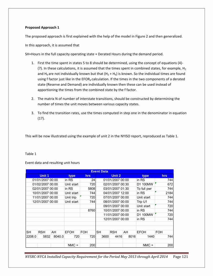
NYSRCNYCA Installed Capacity Requirement for the Period May 2013 through April 2014 Page 121
Proposed Approach 1
The proposed approach is first explained with the help of the model in Figure 2 and then generalized.
In this approach, it is assumed that
SH=Hours in the full capacity operating state + Derated Hours during the demand period.
1. First the time spent in states 5 to 8 should be determined, using the concept of equations (4)‐(7). In these calculations, it is assumed that the times spent in combined states, for example, H2 and H6 are not individually known but that (H2 + H6) is known. So the individual times are found using f factor just like in the EFORd calculation. If the times in the two components of a derated state (Reserve and Demand) are individually known then these can be used instead of apportioning the times from the combined state by the f factor.
2. The matrix N of number of interstate transitions, should be constructed by determining the number of times the unit moves between various capacity states.
3. To find the transition rates, use the times computed in step one in the denominator in equation (17).
This will be now illustrated using the example of unit 2 in the NYISO report, reproduced as Table 1.
Table 1
Event data and resulting unit hours
Event DataUnit 1 type hrs Unit 2 type hrs
in RS 24 in RS 744Unit start 720 D1 100MW 672in RS 5808 To full pwr 744Unit start 744 in RS 2184Unit trip 720 Unit start 744Unit start 744 Trip U1 744
Unit start 7208760 in RS 744
D1 100MW 720in RS 744
SH RSH AH EFOH FOH SH RSH AH EFOH FOH2208.0 5832 8040.0 720 720 3600 4416 8016 1440 744
NMC = 200 NMC = 200
01/01/2007 00:00 01/01/2007 00:0001/02/2007 00:00 02/01/2007 00:3002/01/2007 00:00 03/01/2007 01:3010/01/2007 00:00 04/01/2007 12:0011/01/2007 00:00 07/01/2007 00:0012/01/2007 00:00 08/01/2007 00:00
09/01/2007 00:0010/01/2007 00:0011/01/2007 00:0012/01/2007 00:00

NYSRCNYCA Installed Capacity Requirement for the Period May 2013 through April 2014 Page 122
The computed values of f factors from the appendix B [2] are
ff = 0.70829
fp = 0.44910
Using the concepts of equations (4)‐(7), the time spent in various states are as follows
State 1: Cap=1.0
Time= SH ‐ Derated hours x fp = 3600 ‐ 1392 x 0.44910 =2975
State 2: Cap =0.5
Time= Derated hours x fp = 1392 x 0.4491=625
State 3= Cap=0
Time = FOH x ff = 744 x 0.70829 = 527
So transition rates are
1‐2 = 2/2975 = 0.00067227
1‐3 = 1/2975 = 0.00033613
2‐1 = 2/625 = 0.0032
3‐1 = 1/527 = 0.001898
Using these transition rates, state probabilities are,
P1 = 0 .721
P2 = 0.151
P3 = 0.128
And so,
EFORd = 0.151 x 0.5 + 0.128 = 0.2035
This is about the same as calculated by NYISO formula.
Now the approach can be generalized as follows:
1. Let there be n capacity states of the unit, state 1 with capacity of 1 pu, state n with 0 pu and states 2 to n‐1 as derated states.
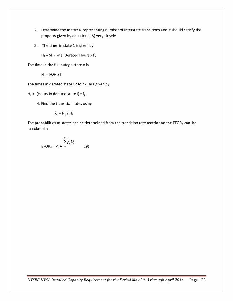
NYSRCNYCA Installed Capacity Requirement for the Period May 2013 through April 2014 Page 123
2. Determine the matrix N representing number of interstate transitions and it should satisfy the property given by equation (18) very closely.
3. The time in state 1 is given by
H1 = SH‐Total Derated Hours x fp
The time in the full outage state n is
Hn = FOH x ff
The times in derated states 2 to n‐1 are given by
Hi = (Hours in derated state i) x fp
4. Find the transition rates using
λij = Nij / Hi
The probabilities of states can be determined from the transition rate matrix and the EFORd can be calculated as
EFORd = Pn +
1
2
n
i iirP
−
=∑
(19)

NYSRCNYCA Installed Capacity Requirement for the Period May 2013 through April 2014 Page 124
Proposed Approach 2
According to the NERC data collection,
SH= Hours in full operating state + Derated Hours
Here the derated hours represent the hours during demand but during the reserve shutdown, distinction between various derated states and full capacity is not reported. In this case the approach can be slightly modified as follows.
1. Let there be n capacity states of the unit, state 1 with capacity of 1 pu, state n with 0 pu and states 2 to n‐1 as derated states.
2. Determine the matrix N representing number of interstate transitions and it should satisfy the property given by equation (18) very closely.
3. The time in state 1 is given by
H1 = SH‐Total Derated Hours
The time in the full outage state n is
Hn = FOH x ff
The time in derated states 2 to n‐1 are given by
Hi = Hours in derated state i
4. Find the transition rates using
λij = Nij / Hi
The probabilities of states can be determined from the transition rate matrix and the EFORd can be calculated as
EFORd = Pn +
1
2
n
i ipi
fr P−
=∑
(20)
Note: It should be observed that these approaches have the following effect. The time used in the denominator of the transition rates from a given state to lower capacity states is actually the service time in that state. For example for state 1, the time used is the time of service in the full capacity state. The time for the repair process is the repair time during the demand period. This will make the conditional repair times shorter than the full repair times or conditional repair rates higher. This is reasonable since only part of the repair may be done during the demand period and remaining repair may be accomplished during reserve shut down.
Calculation Examples of Approach 2

NYSRCNYCA Installed Capacity Requirement for the Period May 2013 through April 2014 Page 125
Two examples are used here to illustrate this approach, one from the NYISO report [2] and the other from the ConEdison report [3].
NYISO Example
Again we use the example of unit 2 in NYISO report [2] but assume that the derated hours are on demand only.
ff = 0.70829
fp = 0.44910
Using the concepts of equations (4)‐(7), the time spent in various states will be as follows.
State 1: Cap=1.0
Time= SH ‐ Derated hours = 3600 ‐ 1392 = 2208
State 2: Cap =0.5
Time= Derated hours = 1392
State 3= Cap=0
Time = FOH x ff = 744 x 0.70829 = 527
So transition rates are
1‐2 = 2/2208 = 0.0009058
1‐3 = 1/2208 = 0.0004529
2‐1 = 2/1392 = 0.00143678
3‐1 = 1/527 = 0.00189753
Using these transition rates, state probabilities are
P1 = 0 .53501
P2 = 0 .33729
P3 = 0 .12770
And so using equation (20)
EFORd = 0.33729 x 0.5 x 0.44910 + 0.12770 = 0.2034
which is exactly the same as using NYISO formula.
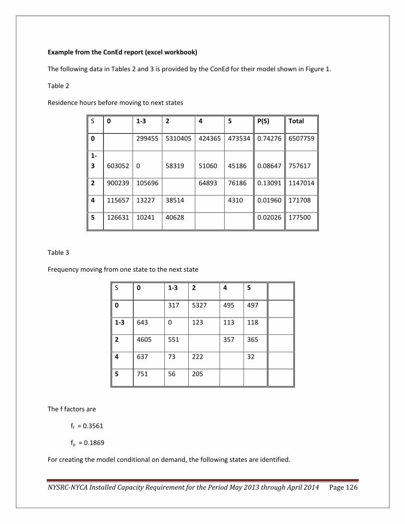
NYSRCNYCA Installed Capacity Requirement for the Period May 2013 through April 2014 Page 126
Example from the ConEd report (excel workbook)
The following data in Tables 2 and 3 is provided by the ConEd for their model shown in Figure 1.
Table 2
Residence hours before moving to next states
S 0 1‐3 2 4 5 P(S) Total
0 299455 5310405 424365 473534 0.74276 6507759
1‐3 603052 0 58319 51060 45186 0.08647 757617
2 900239 105696 64893 76186 0.13091 1147014
4 115657 13227 38514 4310 0.01960 171708
5 126631 10241 40628 0.02026 177500
Table 3
Frequency moving from one state to the next state
S 0 1‐3 2 4 5
0 317 5327 495 497
1‐3 643 0 123 113 118
2 4605 551 357 365
4 637 73 222 32
5 751 56 205
The f factors are
ff = 0.3561
fp = 0.1869
For creating the model conditional on demand, the following states are identified.

NYSRCNYCA Installed Capacity Requirement for the Period May 2013 through April 2014 Page 127
State in the conditional model Original state in Figure 1
State 1 : Cap = 1.0 pu State 2 in Figure 1
State 2 : Cap = 0.8 pu State 4 in Figure 1
State 3 : Cap = 0.65 pu State 5 in Figure 1
State 4 : Cap = 0 pu State 3 in Figure 1
The matrix N of transition frequencies and state times for the conditional model can be created as shown in Table 4. The number of transitions from the new state 1 to other new states represents the transitions from the old states 2 and 0 to the respective states. Similarly number of transitions from new state 4 to other new states represents the transitions from old states 1 and 3 to the respective states. The column sum in the N matrix gives the frequency of entering the state and the row sum gives the frequency of exiting from the state. In Table 4, the frequency balance is very closely maintained. The time spent in the new state 1 is the time in old state 2 and the time in new state 4 is the time in old state 3.
So for new states
H1 = Time in old State 2
= 1147014
H2 = Time in old state 4
= 171708
H3= Time in old state 5
=177500
H4 = (Time in old state 1‐3 ) x ff
=757617 x 0.3561
= 269787

NYSRCNYCA Installed Capacity Requirement for the Period May 2013 through April 2014 Page 128
Table 4
Transition frequency matrix N and state times Hi for the conditional model
State 1 2 3 4 Row Sum Hi Pi
1 0 852 862 868 2582 1147014 0.649495
2 859 0 32 73 964 171708 0.097229
3 956 0 0 56 1012 177500 0.100509
4 766 113 118 0 997 269787 0.152766
Column Sum 2581 965 1012 997 1766009
The transition rates can now be calculated using
λij = Nij / Hi
and are shown in Table 5
Table 5
Transition rate matrix and state probabilities:
State 1 2 3 4 Pi
1 ‐0.002251 0.000743 0.000752 0.000757 0.6494
2 0.0005003 ‐0.005614 0.000186 0.000425 0.0973
3 0.005386 0 ‐0.005701 0.000315 0.1005
4 0.002839 0.000419 0.000437 ‐0.003696 0.1528
It can be seen that the state probabilities obtained in Table 5 using the transition rate matrix are the same as those obtained in Table 4 using the fraction of time spent in the state.
Also using equation (20),
EFORd = P4 + P2 x fp x r2 +P3 x fp x r3

NYSRCNYCA Installed Capacity Requirement for the Period May 2013 through April 2014 Page 129
= 0.1528 + 0.0973 x 0.1869 x (1‐0.8) + 0.1005 x 0.1869 x (1‐0.65)
= 0.1630
Using NYISO formula,
FOH = 757617
EFOH = 171708 x 0.2 + 177500 x 0.35 + 757617
= 854083.6
EFORd = (757617 x 0.3561 + 0.1869 x (854083.6‐757617)) / (1496222 + 757617 x 0.3561)
= 0.1630
So the EFORd calculated from the transition rate matrix and the NYISO formula are the same.
Concluding Remarks
1. Embedded in the EFORd calculation are the following three steps:
‐ Finding times spent in various states during demand
‐ Converting these times into conditional probabilities
‐ Adjusting the times in derated states to equivalent times in the full forced outage state
2. Under the present state of data collection, it is appropriate to assume that the conditional probabilities calculated for EFORd procedure are the bench mark. This is not because EFORd calculation is the ‘absolute truth’ but because that is the practice.
3. For the LOLE calculations using MARS or a similar program to be consistent with the EFORd calculations, transition rate matrix should maintain the conditional state probabilities used in the EFORd calculation.
4. It should be kept in mind that MARS and similar programs do not have mechanisms for starting units in response to demand or shutting down when not needed. Therefore, these programs essentially assume the units running or in service or in demand all the time.
5. To be consistent with this assumption of the units running all the time, models conditional on the demand should to be used.
6. The EFORd calculation formula is based on the conditional probabilities of the states and these conditional probabilities should be assumed as a good estimate of the performance. So the transition rate matrix should be constructed to maintain these conditional probabilities. The

NYSRCNYCA Installed Capacity Requirement for the Period May 2013 through April 2014 Page 130
conditional approach used in the 4‐state model that forms the basis of EFORd calculations was in fact proposed to deal with the assumption of units running all the time.
7. The NYISO true‐up approach may give correct EFORd , but it does not allow the conditional probabilities of the individual states to stay consistent with those required for EFORd and assumed as benchmark. Therefore, while it may give correct EFORD, the LOLE calculation using MARS may be distorted. The amount of distortion will depend on the system characteristics and will vary from one study to the other.
8. The ConEd approach assumes a reserve shut down state which is assumed to be full capacity but without any exposure to failure. To correctly use this model, the program needs to have unit start and shut down capability. As explained in the text, just assigning full capacity to the reserve state will over estimate the unit availability when used in MARS or similar programs.
9. Two approaches have been proposed in this report to generate the transition rate matrix that will yield conditional probabilities of individual states to be consistent with the EFORd formula. Further they have been illustrated using examples from the NYISO and ConEd reports. The underlying philosophy of these approaches is the same but they differ on the nature of data availability for the derated states. Since in these approaches, the conditional probabilities stay consistent with the conditional approach used for EFORd these approaches are suitable for use with MARS.
References
1. IEEE Committee, “A four state model for estimation of outage risk for units in peaking service”, IEEE Task Group on Model for Peaking Units of the Application of Probability Methods Subcommittee, IEEE Transactions, PAS‐91 (1972), pp. 618‐27.
2. Adjustment of Event‐Generated EFORs to Mach EFORds in Resource Adequacy Studies, ISO New York, Nov 2, 2010.
3. Chi‐Hung Kelvin Chu, Carlos Villalba, Developing generating Unit State Transition Rates from Historical Events, ConEdison, Inc.
4. A.D. Patton, C. Singh, M. Sahinoglu, Operating Considerations in Generation Reliability Modeling ‐ An Analytical Approach, IEEE Transactions, PAS‐100, May 1981.
5. A.D. Patton, C. Singh, et al, Modeling of Unit Operating Considerations in Generating Capacity Reliability Evaluation, Vol. 1: Mathematical Models, Computing Methods, and Results, Electric Power Research Institute Report EPRI EL‐2519, Vol. 1, Project 1534‐1, July 1982.
6. C. Singh, Reliability Calculations of Large Systems, Proceedings 1975 Reliability and Maintainability Symposium, 1975.

NYSRCNYCA Installed Capacity Requirement for the Period May 2013 through April 2014 Page 131
7. C. Singh & R. Billinton, Frequency and Duration Concepts in System Reliability Evaluation, IEEE Transactions on Reliability, Vol. R‐24, Bo 1, April 1975.
8. A.D. Patton, C. Singh, et al, Reliability Modeling of Interconnected Systems Recognizing Operating Considerations, EPRI Report EL‐4603, Vol. 1, Project RP 1534‐2, Dec. 1985.
9. IEEE Std 762, IEEE Standard Definitions for Use in Reporting Electric Generating Unit Reliability, Availability, and Productivity, 2008
10. M. P. Bhavaraju,J.A. Hynds, G.A. Nunan,”A method for estimating equivalent forced outage rates of multistae peaking units”, IEEE Transactions on Power Apparatus and Systems, Vol. PAS‐97, No. 6, Nov/Dec 1978
11. C. Singh, Course Notes: Electrical Power System Reliability, Available on URL: http://www.ee.tamu.edu/People/bios/singh/index.htm

NYSRCNYCA Installed Capacity Requirement for the Period May 2013 through April 2014 Page 132
PART II
Implementation and Testing

NYSRCNYCA Installed Capacity Requirement for the Period May 2013 through April 2014 Page 133
Introduction
NYISO gave the implementation of the methodology proposed in Part I to GADS OS. They also gave data on two units to APA to hand calculate so that the results between the software implementation and hand calculation can be compared. This effort can be explained in three parts:
1. Interpretation of the data provided
2. Calculation of the transition rate matrix, and
3. Comparison between the results obtained by computer program and hand calculation implemented using excel workbook.
Data Interpretation
In order to correctly calculate the transition rates of a unit using its historic events‐data, its state durations need to be in a strictly seamless sequence without any overlapping. There will be little difficulty in calculations if the raw data events are in an ideal sequence, i.e., the beginning time of any event is equal to or later than the ending time of its previous event. However, we find that in the raw data there are quite a few records indicating existence of overlapping events. In addition, some records even show discrepancies in the sequence of events, e.g., an event started and ended before the beginning time of its previous event. All these discrepancies in raw data will frustrate the standard programming algorithms and can cause erroneous calculation results. Therefore, suitable pretreatment of the raw data events is necessary. In addition, the specified statistical data after the calculations also need to benchmark those in the performance data. These are actually the principles of the method proposed here. The general flowchart of Data Handling Method is illustrated in Figure 4.

NYSRCNYCA Installed Capacity Requirement for the Period May 2013 through April 2014 Page 134
Figure 4. General flow chart of data handling.
The details of each sub‐level algorithm are illustrated in the following.
Algorithm for Pretreatment Procedure 1: Handling Mistaken Sequence of Events
When events in mistaken sequence are found, their places in the overall event sequence list should be reordered. Unless all mistaken sequence records of a unit are corrected, the next Pretreatment Procedure 2 should not begin. The general flowchart of the algorithm of Pretreatment Procedure 1 is illustrated in Figure 5.
Begin
End
Pretreatment Procedure 1: Handling mistaken sequence of events
Pretreatment Procedure 2: Handling overlapping events
Main Procedure: Calculating transition rates

NYSRCNYCA Installed Capacity Requirement for the Period May 2013 through April 2014 Page 135
Figure 5. Flowchart of Pretreatment Procedure 1
Algorithm for Pretreatment Procedure 2: Handling Overlapping Events
After Pretreatment Procedure 1, we are guaranteed to have a set of sequential events without mistaken orders. Nevertheless, overlapping events could still exist and need to be properly handled. In order to benchmark statistics in the performance data, we need to follow some rules to appropriately handle the overlapping events.
Firstly, we classify all events into the following priority levels:
1st priority events: Forced outages (Ux, SF)
2nd priority events: Reserve shutdown (RS)
3rd priority events: Deratings (Dx, PD)
4th priority events: Maintenance (PO, PE, MO)
Begin
End
Initialization of Pretreatment Procedure 1: Set event sequence order index i = 1
Other necessary initializations
i = i + 1
Event (i) started before the beginning time
of Event (i-1) ?
Switch the sequence orderof Event (i) and Event (i-1)
i = i − 1
Yes
No
Event (i) = last event
Yes
No

NYSRCNYCA Installed Capacity Requirement for the Period May 2013 through April 2014 Page 136
5th priority events: Full capacity (NC, full capacity being gaps between adjacent events)
The different kinds of events in the same priority level are observed not to be overlapping data records. For any two adjacent overlapping events from different priority levels, four rules for appropriate handling are summarized as follows.
(1) If the lower priority event started before the beginning time of the higher priority event, and the lower priority event ended before or at the same time as the ending time of the higher priority event, adjust the ending time of the lower priority event benchmarking the beginning time of the higher priority event. This rule is illustrated as in Figure 6.
Figure 6. Rule 1
(2) If the lower priority event started before the beginning time of the higher priority event, and the lower priority event ended after the ending time of the higher priority event, replace the original lower priority event by two new separate events. For the first new event, inherit the beginning time of the original lower priority event as its beginning time, and adopt the beginning time of the higher priority event as its ending time. For the second new event, inherit the ending time of the original lower priority event as its ending time, and adopt the ending time of the higher priority event as its beginning time. This rule is illustrated as in Figure 7.
Lower Priority
Lower Priority
Higher Priority (Event 2)
Higher Priority (Event 2)
Beginning Time
Ending Time
Beginning Time
Ending Time
Beginning Time
Beginning Time
Lower Priority
Higher Priority (Event 2)
Ending Time
Ending Time

NYSRCNYCA Installed Capacity Requirement for the Period May 2013 through April 2014 Page 137
Figure 7. Rule 2
(3) If the lower priority event started at the same time as or after the beginning time of the higher priority event, and the lower priority event ended before or at the same time as the ending time of the higher priority event, invalidate the lower priority event for transition rate calculation. This rule is illustrated as in Figure 8.
Lower Priority (Event 2)
Higher Priority (Event 1)
Beginning Time
Beginning Time
Ending Time
Ending Time
Lower Priority (Event 2)
Higher Priority (Event 1)
Lower Priority (Event 2)
Higher Priority (Event 1)
Lower Priority (Event 2)
Higher Priority (Event 1)
Higher Priority (Event 1)
Beginning Time
Ending Time
Lower Priority (Event 1)
Higher Priority (Event 2)
Beginning Time
Ending Time 1-1
Beginning Time
Ending Time
Beginning Time 1-1
Beginning Time
Lower Priority (Event 1-1)
Higher Priority (Event 2)
Ending Time
Ending Time
Lower Priority (Event 1-2)
Beginning Time 1-2
Ending Time 1-2

NYSRCNYCA Installed Capacity Requirement for the Period May 2013 through April 2014 Page 138
Figure 8. Rule 3
(4) If the lower priority event started at the same time as or after the beginning time of the higher priority event, and the lower priority event ended after the ending time of the higher priority event, adjust the beginning time of the lower priority event benchmarking the ending time of the higher priority event. This rule is illustrated as in Figure 9.
Figure 9. Rule 4
The general flowchart of the algorithm of Pretreatment Procedure 2 is illustrated as in Figure 10.
Lower Priority (Event 2)
Higher Priority (Event 1)
Beginning Time
Beginning Time
Ending Time
Ending Time
Lower Priority (Event 2)
Higher Priority (Event 1)
Beginning Time
Ending Time
Beginning Time
Ending Time
Lower Priority (Event 2)
Higher Priority (Event 1)

NYSRCNYCA Installed Capacity Requirement for the Period May 2013 through April 2014 Page 139
Figure 10. General flow chart of Pretreatment Procedure 2
Algorithm of Main Procedure: Calculating Transition Rates
After Pretreatment Procedure 2, we are guaranteed to have an ideal set of sequential events, i.e., a strict sequence without any overlapping. Now there should be hardly any difficulty in counting the duration of each state and calculating the transition rates of a unit.
One point that needs to be paid attention to is that the majority of the full‐capacity states exist in the form of time gaps between adjacent events rather than an explicit full‐capacity event in the sequential event list. In addition, we do find in the raw data a few cases that the time gap between two adjacent events is very small (1 minute). This could possibly be due to human errors. Thus, we add an additional rule besides the standard procedure to calculate transition rates as follows.
Rule of Seamlessness:
After Pretreatment Procedure 2, if the time gap between any two adjacent events is no greater than 1 minute or any other specified duration, it will be ignored and the two events are considered as
Begin
End
Initialization of Pretreatment Procedure 2: Set event sequence order index i = 1
Other necessary initializations
i = i + 1
Event (i+1) started before the ending time
of Event (i) ?
Adjust Event (i) or Event (i+1) using the four rules of
handling overlapping events
Yes
No
Event (i) = last event
Yes
No

NYSRCNYCA Installed Capacity Requirement for the Period May 2013 through April 2014 Page 140
neighboring events. Otherwise, the time gap will be regarded as an event of full‐capacity state existing between the two adjacent events.
Another point that also needs to be paid attention to is that all the derating states remaining in the sequential event list after Pretreatment Procedure 2 are already separate from reserve shutdown states. Hence, these remaining derating states are now regarded in demand. When counting the total durations of these derating states for calculating transition rates, the fp factor is no longer necessary. However, the ff factor is still needed since there is no good way to distinguish in‐demand or not‐in‐demand states when a unit is actually in a forced outage status.
The general flowchart of the algorithm of the Main Procedure is illustrated as in Figure 11.
Begin
End
Initialization of Main Procedure: Set event sequence order index i = 1
Other necessary initializations
i = i + 1
Is this gap greater than 1 minute ?
Set the gap as Event (i+1) of full-capacity state
Standard procedure for counting transition numbers and state durations
Yes
No
Event (i) = last event
Yes
No
Is a gap between the ending time of Event (i) and
the beginning time of Event (i+1) ?
Yes
No
Standard procedure for calculating transition rates

NYSRCNYCA Installed Capacity Requirement for the Period May 2013 through April 2014 Page 141
Figure 11. Summary of Data Handling Method
If all the rules and algorithms of Data Handling Method are appropriately followed, the transition rates of a unit can be obtained correctly in addition to a set of statistical data capable of benchmarking those in the performance data.
Calculation of Transition Rate Matrix
In calculating the transition rate matrix, the first step is to define derated states in addition to the full capacity and forced out states. In the two units analyzed two derated capacity states were introduced. For this first the time‐weighted mean capacity of derated states was computed. Then the states with capacity greater than this value were put into the first derated state and those with capacity less than this were included in the second derated state. Then the mean capacities of these two states were calculated.
The two pieces of information needed for transition rate matrix are the times spent in four states during demand and the number of transitions between these states. The calculation of times once the data has been pretreated is relatively straightforward. For calculating the interstate transitions, the simple rule is that starting in a demand state, determine the next demand state to find the transition. The interstate transitions are given in column W of the spreadsheet. First the number of interstate transitions is given and then it is converted to transition rate matrices for approach 1 and 2. The number of transitions into and out a state need to be balanced as explained in the Part 1 on the basic theory. If the ending state is the same as the beginning state, then these numbers will be balanced, otherwise a transition at the end may be added to balance.
The calculations are given in the spread sheets along with notes and formulae.
Verification of GADS OS Code
The transition rate matrices produced by the computer program were compared with those produced by the spreadsheets and in the two units analyzed, match was obtained.

EXHIBIT 2
NYSRC RESOLUTION ADOPTINGTHE IRM FOR THE 2013-2014 CAPACITY YEAR

NEW YORK STATE RELIABILITY COUNCIL, L.L.C.APPROVAL OF NEW YORK CONTROL AREA
INSTALLED CAPACITY REQUIREMENT FOR THE PERIODMAY 1, 2013 THROUGH APRIL 30, 2014
1. WHEREAS, reliable electric service is critical to the economic and social welfare ofthe millions of residents and businesses in the State of New York; and
2. WHEREAS, the reliable and efficient operation of the New York State PowerSystem is fundamental to achieving and maintaining reliability of power supply; and
3. WHEREAS, The New York State Reliability Council, L.L.C.’s (NYSRC) principalmission is to establish Reliability Rules for use by the New York IndependentSystem Operator (NYISO) to maintain the integrity and reliability of the NYS PowerSystem; and
4. WHEREAS, the NYSRC is responsible for determining the New York Control Area(NYCA) annual Installed Capacity Requirement (ICR); and
5. WHEREAS, the New York Control Area Installed Capacity Requirements for thePeriod May 2013 through April 2014, Technical Study Report (Technical StudyReport) dated December 7, 2012, prepared by the NYSRC Installed CapacitySubcommittee, concludes that, under base case conditions, the required NYCAinstalled reserve margin (IRM) for the May1, 2013 through April 30, 2014Capability Year is 17.1%; and
6. WHEREAS, in light of the Technical Study Report results, the modeling andassumption changes made to simulate actual operating conditions and systemperformance as set forth in Table 6-1 of the Technical Study Report, the numeroussensitivity studies evaluated, and other relevant factors;
7. NOW, THEREFORE BE IT RESOLVED, that in consideration of the factorsdescribed above, the NYSRC finds that an IRM requirement at 17.0%, whichequates to an ICR of 1.17 times the forecasted NYCA 2013 peak load, will satisfythe criteria for resource adequacy set forth in the NYSRC’s Reliability Rule A-R1and hereby sets the NYCA IRM requirement for the May 1, 2013 to April 30, 2014Capability Year at 17.0%.