Embed Size (px)
Citation preview
Chapter 6
State Feedback
Intuitively, the state may be regarded as a kind of information storage or
memory or accumulation of past causes. We must, of course, demand that
the set of internal states Σ be sufficiently rich to carry all information about
the past history of Σ to predict the effect of the past upon the future. We do
not insist, however, that the state is the least such information although this
is often a convenient assumption.
R. E. Kalman, P. L. Falb and M. A. Arbib, 1969 [KFA69].
This chapter describes how feedback of a system’s state can be usedshape the local behavior of a system. The concept of reachability is intro-duced and used to investigate how to “design” the dynamics of a systemthrough assignment of its eigenvalues. In particular, it will be shown thatunder certain conditions it is possible to assign the system eigenvalues toarbitrary values by appropriate feedback of the system state.
6.1 Reachability
One of the fundamental properties of a control system is what set of points inthe state space can be reached through the choice of a control input. It turnsout that the property of “reachability” is also fundamental in understandingthe extent to which feedback can be used to design the dynamics of a system.
Definition
We begin by disregarding the output measurements of the system and fo-cusing on the evolution of the state, given by
dx
dt= Ax + Bu, (6.1)
187
188 CHAPTER 6. STATE FEEDBACK
x0
x(T )
R(x0,≤ T )
(a) (b)
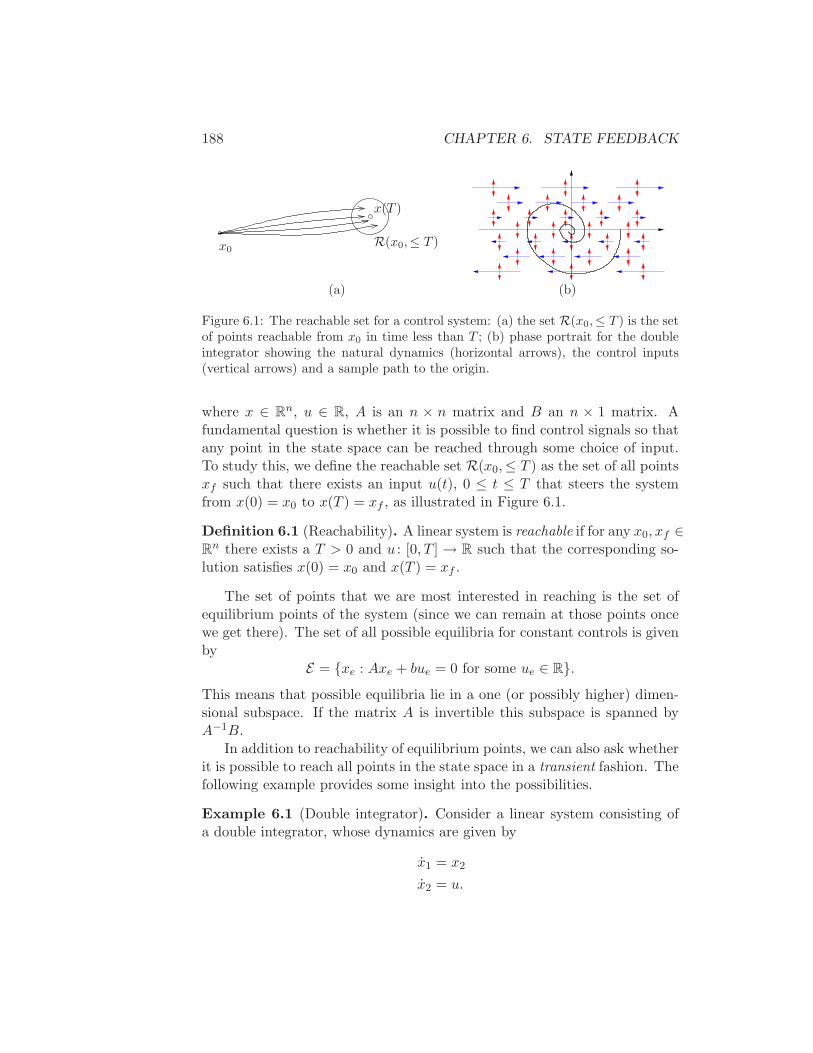
Figure 6.1: The reachable set for a control system: (a) the set R(x0,≤ T ) is the setof points reachable from x0 in time less than T ; (b) phase portrait for the doubleintegrator showing the natural dynamics (horizontal arrows), the control inputs(vertical arrows) and a sample path to the origin.
where x ∈ Rn, u ∈ R, A is an n × n matrix and B an n × 1 matrix. A
fundamental question is whether it is possible to find control signals so thatany point in the state space can be reached through some choice of input.To study this, we define the reachable set R(x0,≤ T ) as the set of all pointsxf such that there exists an input u(t), 0 ≤ t ≤ T that steers the systemfrom x(0) = x0 to x(T ) = xf , as illustrated in Figure 6.1.
Definition 6.1 (Reachability). A linear system is reachable if for any x0, xf ∈R
n there exists a T > 0 and u : [0, T ] → R such that the corresponding so-lution satisfies x(0) = x0 and x(T ) = xf .
The set of points that we are most interested in reaching is the set ofequilibrium points of the system (since we can remain at those points oncewe get there). The set of all possible equilibria for constant controls is givenby
E = {xe : Axe + bue = 0 for some ue ∈ R}.This means that possible equilibria lie in a one (or possibly higher) dimen-sional subspace. If the matrix A is invertible this subspace is spanned byA−1B.
In addition to reachability of equilibrium points, we can also ask whetherit is possible to reach all points in the state space in a transient fashion. Thefollowing example provides some insight into the possibilities.
Example 6.1 (Double integrator). Consider a linear system consisting ofa double integrator, whose dynamics are given by
x1 = x2
x2 = u.
6.1. REACHABILITY 189
Figure 6.1b shows a phase portrait of the system. The open loop dynamics(u = 0) are shown as horizontal arrows pointed to the right for x2 > 0 andthe the left for x2 < 0. The control input is represented by a double arrowin the vertical direction, corresponding to our ability to set the value of x2.The set of equilibrium points E corresponds to the x1 axis, with ue = 0.
Suppose first that we wish to reach the origin from an initial condition(a, 0). We can directly move the state up and down in the phase plane, butwe must rely on the natural dynamics to control the motion to the left andright. If a > 0, we can move the origin by first setting u < 0, which will casex2 to become negative. Once x2 < 0, the value of x1 will begin to decreaseand we will move to the left. After a while, we can set u2 to be positive,moving x2 back toward zero and slowing the motion in the x1 direction. Ifwe bring x2 > 0, we can move the system state in the opposite direction.
Figure 6.1b shows a sample trajectory bringing the system to the origin.Note that if we steer the system to an equilibrium point, it is possible toremain there indefinitely (since x1 = 0 when x2 = 0), but if we go to anyother point in the state space, we can only pass through the point in atransient fashion. ∇
To find general conditions under which a linear system is reachable, wewill first give a heuristic argument based on formal calculations with impulsefunctions. We note that if we can reach all points in the state space throughsome choice of input, then we can also reach all equilibrium points. Hencereachability of the entire state space implies reachability of all equilibriumpoints.
Testing for Reachability
When the initial state is zero, the response of the state to a unit step in theinput is given by
x(t) =
∫ t
0eA(t−τ)Bdτ = A−1(eAt − I)B (6.2)
The derivative of a unit step function is the impulse function, δ(t), defined inSection 5.2. Since derivatives are linear operations, it follows (see Exercise 7)that the response of the system to an impulse function is thus the derivativeof equation (6.2) (i.e., the impulse response),
dx
dt= eAtB.
190 CHAPTER 6. STATE FEEDBACK
Similarly we find that the response to the derivative of a impulse functionis
d2x
dt2= AeAtB.
Continuing this process and using the linearity of the system, the input
u(t) = α1δ(t) + α2δ(t) + αδ(t) + · · · + αnδ(n−1)(t)
gives the state
x(t) = α1eAtB + α2AeAtB + α3A
2eAtB + · · · + αnAn−1eAtB.
Hence, right after the initial time t = 0, denoted t = 0+, we have
x(0+) = α1B + α2AB + α3A2B + · · · + αnAn−1B.
The right hand is a linear combination of the columns of the matrix
Wr =
B AB · · · An−1B
. (6.3)
To reach an arbitrary point in the state space we thus require that there aren linear independent columns of the matrix Wr. The matrix is called thereachability matrix.
An input consisting of a sum of impulse functions and their derivativesis a very violent signal. To see that an arbitrary point can be reached withsmoother signals we can also argue as follows. Assuming that the initialcondition is zero, the state of a linear system is given by
x(t) =
∫ t
0eA(t−τ)Bu(τ)dτ =
∫ t
0eAτBu(t − τ)dτ.
It follows from the theory of matrix functions, specifically the Cayley-Hamiltontheorem [Str88] that
eAτ = Iα0(τ) + Aα1(τ) + · · · + An−1αn−1(τ),
where αi(τ) are scalar functions, and we find that
x(t) = B
∫ t
0α0(τ)u(t − τ) dτ + AB
∫ t
0α1(τ)u(t − τ) dτ+
· · · + An−1B
∫ t
0αn−1(τ)u(t − τ) dτ.
Again we observe that the right hand side is a linear combination of thecolumns of the reachability matrix Wr given by equation (6.3). This basicapproach leads to the following theorem.
6.1. REACHABILITY 191
l
MF
p
θm
(a) (b)
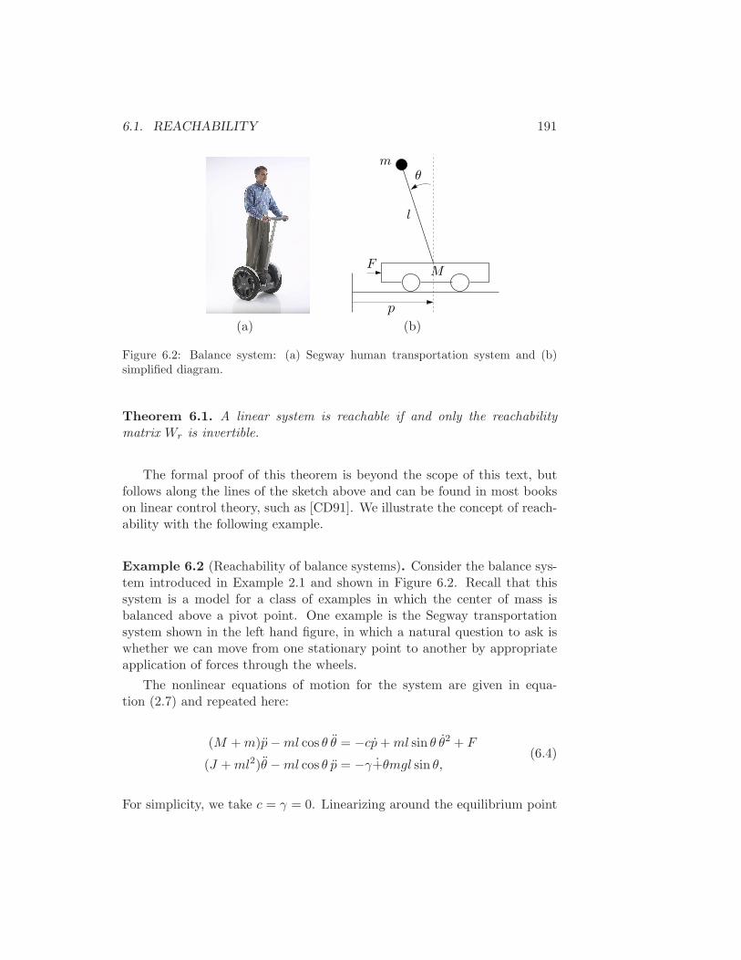
Figure 6.2: Balance system: (a) Segway human transportation system and (b)simplified diagram.
Theorem 6.1. A linear system is reachable if and only the reachability
matrix Wr is invertible.
The formal proof of this theorem is beyond the scope of this text, butfollows along the lines of the sketch above and can be found in most bookson linear control theory, such as [CD91]. We illustrate the concept of reach-ability with the following example.
Example 6.2 (Reachability of balance systems). Consider the balance sys-tem introduced in Example 2.1 and shown in Figure 6.2. Recall that thissystem is a model for a class of examples in which the center of mass isbalanced above a pivot point. One example is the Segway transportationsystem shown in the left hand figure, in which a natural question to ask iswhether we can move from one stationary point to another by appropriateapplication of forces through the wheels.
The nonlinear equations of motion for the system are given in equa-tion (2.7) and repeated here:
(M + m)p − ml cos θ θ = −cp + ml sin θ θ2 + F
(J + ml2)θ − ml cos θ p = −γ+θmgl sin θ,(6.4)
For simplicity, we take c = γ = 0. Linearizing around the equilibrium point
192 CHAPTER 6. STATE FEEDBACK
S
S
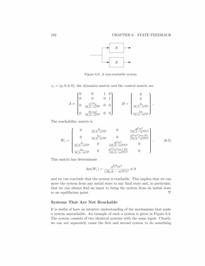
Figure 6.3: A non-reachable system.
xe = (p, 0, 0, 0), the dynamics matrix and the control matrix are
A =
0 0 1 00 0 0 1
0 m2l2gMtJt−m2l2
0 0
0 MtmglMtJt−m2l2
0 0
B =
00
Jt
MtJt−m2l2
lmMtJt−m2l2
,
The reachability matrix is
Wr =
0 Jt
MtJt−m2l20 gl3m3
(MtJt−m2l2)2
0 lmMtJt−m2l2
0 gl2m2(m+M)(MtJt−m2l2)2
Jt
MtJt−m2l20 gl3m3
(MtJt−m2l2)20
lmMtJt−m2l2
0 g2l2m2(m+M)(MtJt−m2l2)2
0
. (6.5)
This matrix has determinant
det(Wr) =g2l4m4
(MtJt − m2l2)46= 0
and we can conclude that the system is reachable. This implies that we canmove the system from any initial state to any final state and, in particular,that we can always find an input to bring the system from an initial stateto an equilibrium point. ∇
Systems That Are Not Reachable
It is useful of have an intuitive understanding of the mechanisms that makea system unreachable. An example of such a system is given in Figure 6.3.The system consists of two identical systems with the same input. Clearly,we can not separately cause the first and second system to do something
6.1. REACHABILITY 193
different since they have the same input. Hence we cannot reach arbitrarystates and so the system is not reachable (Exercise 1).
More subtle mechanisms for non-reachability can also occur. For exam-ple, if there is a linear combination of states that always remains constant,then the system is not reachable. To see this, suppose that there exists arow vector H such that
0 =d
dtHx = H(Ax + Bu) for all u.
Then H is in the left null space of both A and B and it follows that
HWr = H
BAB · · ·An−1B
= 0.
Hence the reachability matrix is not full rank. In this case, if we have aninitial condition x0 and we wish to reach a state xf for which Hx0 6= Hxf ,then since Hx(t) is constant, no input u can move from x0 to xf .
Reachable Canonical Form
As we have already seen in previous chapters, it is often convenient to changecoordinates and write the dynamics of the system in the transformed coor-dinates z = Tx. One application of a change of coordinates is to convert asystem into a canonical form in which it is easy to perform certain types ofanalysis. Once such canonical form is called reachable canonical form.
Definition 6.2 (Reachable canonical form). A linear state space system isin reachable canonical form if its dynamics are given by
dz
dt=
−a1 −a2 −a3 . . . −an
1 0 0 . . . 00 1 0 . . . 0...
. . .. . .
...0 1 0
z +
100...0
u
y =
b1 b2 b3 . . . bn
z.
(6.6)
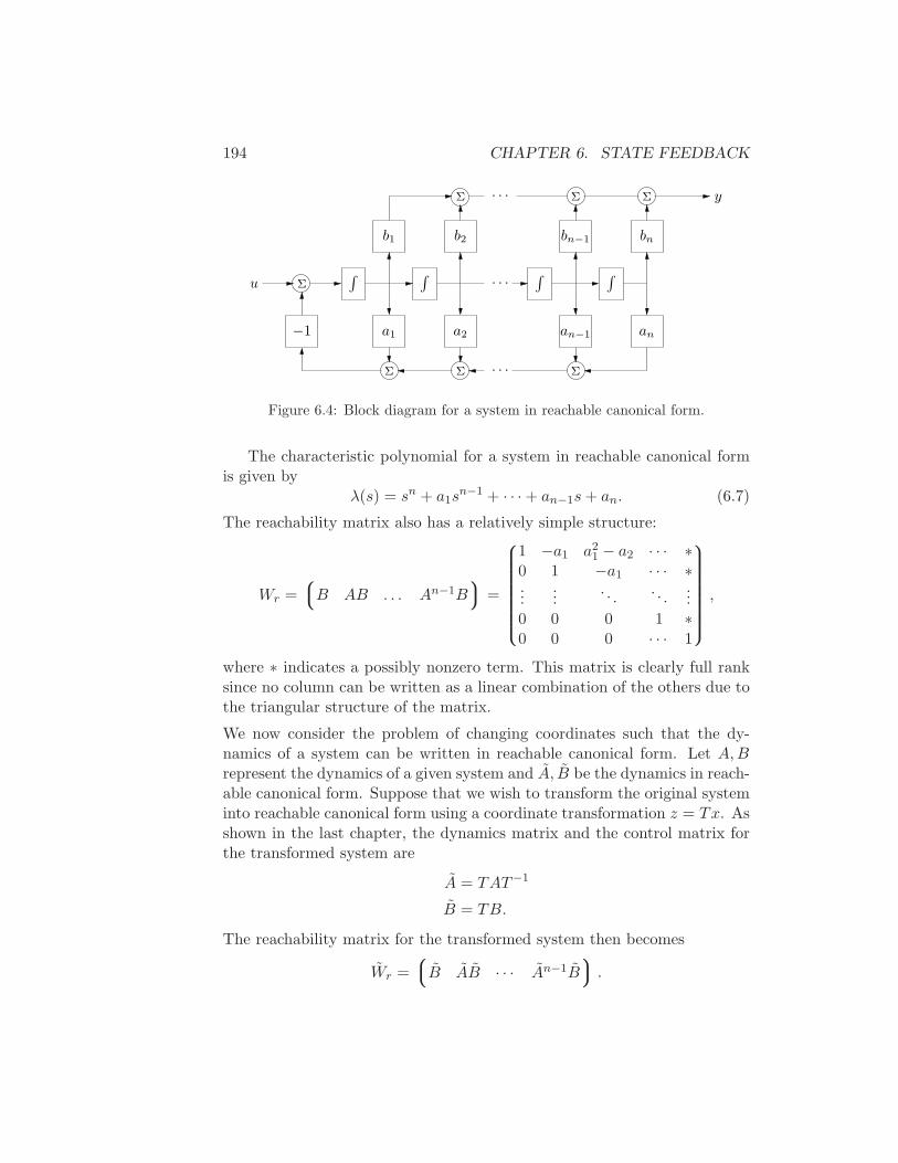
A block diagram for a system in reachable canonical form is shown inFigure 6.4. We see that the coefficients that appear in the A and B matricesshow up directly in the block diagram. Furthermore, the output of thesystem is a simple linear combination of the outputs of the integration blocks.
194 CHAPTER 6. STATE FEEDBACK
Σ
∫
a1
Σ
Σ
b1
−1
∫
u
Σ
a2
Σ
. . .
. . .
. . .
b2
∫
Σ
Σ
an−1 an
bnbn−1
∫
y
Figure 6.4: Block diagram for a system in reachable canonical form.
The characteristic polynomial for a system in reachable canonical formis given by
λ(s) = sn + a1sn−1 + · · · + an−1s + an. (6.7)
The reachability matrix also has a relatively simple structure:
Wr =
B AB . . . An−1B
=
1 −a1 a21 − a2 · · · ∗
0 1 −a1 · · · ∗...
.... . .
. . ....
0 0 0 1 ∗0 0 0 · · · 1
,
where ∗ indicates a possibly nonzero term. This matrix is clearly full ranksince no column can be written as a linear combination of the others due tothe triangular structure of the matrix.
We now consider the problem of changing coordinates such that the dy-namics of a system can be written in reachable canonical form. Let A, Brepresent the dynamics of a given system and A, B be the dynamics in reach-able canonical form. Suppose that we wish to transform the original systeminto reachable canonical form using a coordinate transformation z = Tx. Asshown in the last chapter, the dynamics matrix and the control matrix forthe transformed system are
A = TAT−1
B = TB.
The reachability matrix for the transformed system then becomes
Wr =
B AB · · · An−1B
.
6.1. REACHABILITY 195
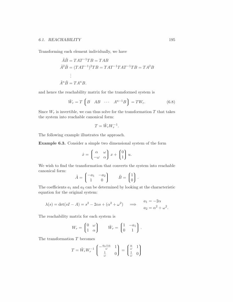
Transforming each element individually, we have
AB = TAT−1TB = TAB
A2B = (TAT−1)2TB = TAT−1TAT−1TB = TA2B
...
AnB = TAnB.
and hence the reachability matrix for the transformed system is
Wr = T
B AB · · · An−1B
= TWr. (6.8)
Since Wr is invertible, we can thus solve for the transformation T that takesthe system into reachable canonical form:
T = WrW−1r .
The following example illustrates the approach.
Example 6.3. Consider a simple two dimensional system of the form
x =
α ω−ω α
x +
01
u.
We wish to find the transformation that converts the system into reachablecanonical form:
A =
−a1 −a2
1 0
B =
10
.
The coefficients a1 and a2 can be determined by looking at the characteristicequation for the original system:
λ(s) = det(sI − A) = s2 − 2αs + (α2 + ω2) =⇒a1 = −2α
a2 = α2 + ω2.
The reachability matrix for each system is
Wr =
0 ω1 α
Wr =
1 −a1
0 1
.
The transformation T becomes
T = WrW−1r
−a1+αω 1
1ω 0
=
αω 1
1ω 0
196 CHAPTER 6. STATE FEEDBACK
and hence the coordinates
z1
z2
= Tx =
αωx1 + x2
x2
put the system in reachable canonical form. ∇
We summarize the results of this section in the following theorem.
Theorem 6.2. Let (A, B) be the dynamics and control matrices for a reach-
able system. Then there exists a transformation z = Tx such that in the
transformed coordinates the dynamics and control matrices are in reachable
canonical form (6.6) and the characteristic polynomial for A is given by
det(sI − A) = sn + a1sn−1 + · · · + an−1s + an.
One important implication of this theorem is that for any reachablesystem, we can always assume without loss of generality that the coordinatesare chosen such that the system is in reachable canonical form. This isparticularly useful for proofs, as we shall see later in this chapter.
6.2 Stabilization by State Feedback
The state of a dynamical system is a collection of variables that permitsprediction of the future development of a system. We now explore the ideaof designing the dynamics a system through feedback of the state. Wewill assume that the system to be controlled is described by a linear statemodel and has a single input (for simplicity). The feedback control will bedeveloped step by step using one single idea: the positioning of closed loopeigenvalues in desired locations.
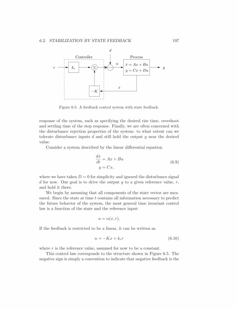
Figure 6.5 shows a diagram of a typical control system using state feed-back. The full system consists of the process dynamics, which we take tobe linear, the controller elements, K and kr, the reference input, r, andprocesses disturbances, d. The goal of the feedback controller is to regulatethe output of the system, y, such that it tracks the reference input in thepresence of disturbances and also uncertainty in the process dynamics.
An important element of the control design is the performance specifi-cation. The simplest performance specification is that of stability: in theabsence of any disturbances, we would like the equilibrium point of thesystem to be asymptotically stable. More sophisticated performance speci-fications typically involve giving desired properties of the step or frequency
6.2. STABILIZATION BY STATE FEEDBACK 197
Process
y
x
uΣ
x = Ax + Bu
y = Cx + Du
d
Σ
−K
krr
Controller
Figure 6.5: A feedback control system with state feedback.
response of the system, such as specifying the desired rise time, overshootand settling time of the step response. Finally, we are often concerned withthe disturbance rejection properties of the system: to what extent can wetolerate disturbance inputs d and still hold the output y near the desiredvalue.
Consider a system described by the linear differential equation
dx
dt= Ax + Bu
y = Cx,(6.9)
where we have taken D = 0 for simplicity and ignored the disturbance signald for now. Our goal is to drive the output y to a given reference value, r,and hold it there.
We begin by assuming that all components of the state vector are mea-sured. Since the state at time t contains all information necessary to predictthe future behavior of the system, the most general time invariant controllaw is a function of the state and the reference input:
u = α(x, r).
If the feedback is restricted to be a linear, it can be written as
u = −Kx + krr (6.10)
where r is the reference value, assumed for now to be a constant.
This control law corresponds to the structure shown in Figure 6.5. Thenegative sign is simply a convention to indicate that negative feedback is the
198 CHAPTER 6. STATE FEEDBACK
normal situation. The closed loop system obtained when the feedback (6.9)is applied to the system (6.10) is given by
dx
dt= (A − BK)x + Bkrr (6.11)
We attempt to determine the feedback gain K so that the closed loop systemhas the characteristic polynomial
p(s) = sn + p1sn−1 + · · · + pn−1s + pn (6.12)
This control problem is called the eigenvalue assignment problem or “poleplacement” problem (we will define “poles” more formally in a later chapter).
Note that the kr does not affect the stability of the system (which isdetermined by the eigenvalues of A−BK), but does affect the steady statesolution. In particular, the equilibrium point and steady state output forthe closed loop system are given by
xe = −(A − BK)−1Bkrr ye = Cxe,
hence kr should be chosen such that ye = r (the desired output value). Sincekr is a scalar, we can easily solve to show
kr = −1/(
C(A − BK)−1B)
. (6.13)
Notice that kr is exactly the inverse of the zero frequency gain of the closedloop system.
Using the gains K and kr, we are thus able to design the dynamics of theclosed loop system to satisfy our goal. To illustrate how to such construct astate feedback control law, we begin with a few examples that provide somebasic intuition and insights.
Examples
Example 6.4 (Vehicle steering). In Example 5.12 we derived a normal-ized linear model for vehicle steering. The dynamics describing the lateraldeviation where given by
A =
0 10 0
B =
α1
C =
1 0
D = 0.
6.2. STABILIZATION BY STATE FEEDBACK 199
The reachability matrix for the system is thus
Wr =
B AB
=
α 11 0
.
The system is reachable since det Wr = −1 6= 0.We now want to design a controller that stabilizes the dynamics and
tracks a given reference value r of the lateral position of the vehicle. To dothis we introduce the feedback
u = −Kx + krr = −k1x1 − k2x2 + krr,
and the closed loop system becomes
dx
dt= (A − BK)x + Bkrr =
−αk1 1 − αk2
−k1 −k2
x +
αkr
kr
r
y = Cx + Du =
1 0
x.
(6.14)
The closed loop system has the characteristic polynomial
det (sI − A + BK) = det
s + αk1 αk2 − 1k1 s + k2
= s2 + (αk1 + k2)s + k1.
Suppose that we would like to use feedback to design the dynamics of thesystem to have a characteristic polynomial
p(s) = s2 + 2ζcωcs + ω2c .
Comparing this with the characteristic polynomial of the closed loop systemwe see that the feedback gains should be chosen as
k1 = ω2c , k2 = 2ζcωc − αω2
c .
To have x1 = r in the steady state it must be required that the parameterkr equal to k1 = ω2
c . The control law can thus be written as
u = k1(r − x1) − k2x2 = ω2c (r − x1) − (2ζcωc − αω2
c )x2.
∇
The example of the vehicle steering system illustrates how state feedbackcan be used to set the eigenvalues of the closed loop system to arbitraryvalues. The next example demonstrates that this is not always possible.
200 CHAPTER 6. STATE FEEDBACK
Example 6.5 (An unreachable system). Consider the system
dx
dt=
0 10 0
x +
10
u
y =
1 0
x
with the control lawu = −k1x1 − k2x2 + krr.
The closed loop system is
dx
dt=
−k1 1 − k2
0 0
x +
kr
0
r.
This system has the characteristic polynomial
det
s + k1 −1 + k2
0 s
= s2 + k1s = s(s + k1),
which has zeros at s = 0 and s = −k1. Since one closed loop eigenvalue isalways equal to s = 0, independently of our choice of gains, it is not possibleto obtain an arbitrary characteristic polynomial.
A visual inspection of the equations of motion shows that this systemalso has the property that it is not reachable. In particular, since x2 = 0,we can never steer x2 between one value and another. Computation of thereachability matrix Wr verifies that the system is not reachable. ∇
The reachable canonical form has the property that the parameters ofthe system are the coefficients of the characteristic equation. It is thereforenatural to consider systems on this form when solving the eigenvalue assign-ment problem. In the next example we investigate the case when the systemis in reachable canonical form.
Example 6.6 (System in reachable canonical form). Consider a system inreachable canonical form, i.e,
dz
dt= Az + Bu =
−a1 −a2 −a3 . . . −an
1 0 0 . . . 00 1 0 . . . 0...
. . .. . .
...0 1 0
z +
10...00
u
y = Cz =
b1 b2 · · · bn
z.
(6.15)
6.2. STABILIZATION BY STATE FEEDBACK 201
The open loop system has the characteristic polynomial
det(sI − A) = sn + a1sn−1 + · · · + an−1s + an,
as we saw in Example 6.6.Before making a formal analysis we will investigate the block diagram
of the system shown in Figure 6.4. The characteristic polynomial is givenby the parameters ak in the figure. Notice that the parameter ak can bechanged by feedback from state xk to the input u. It is thus straight forwardto change the coefficients of the characteristic polynomial by state feedback.
Having developed some intuition we will now proceed formally. Intro-ducing the control law
u = −Kz + krr = −k1z1 − k2z2 − · · · − knzn + krr, (6.16)
the closed loop system becomes
dz
dt=
−a1 − k1 −a2 − k2 −a3 − k3 . . . −an − kn
1 0 0 . . . 00 1 0 . . . 0...
. . .. . .
...0 1 0
z +
kr
00...0
r
y =
bn · · · b2 b1
z.
(6.17)The feedback changes the elements of the first row of the A matrix, whichcorresponds to the parameters of the characteristic equation. The closedloop system thus has the characteristic polynomial
sn + (al + k1)sn−1 + (a2 + k2)s
n−2 + · · · + (an−1 + kn−1)s + an + kn.
Requiring this polynomial to be equal to the desired closed loop polyno-mial (6.12) we find that the controller gains should be chosen as
k1 = p1 − a1
k2 = p2 − a2
...
kn = pn − an.
This feedback simply replaces the parameters ai in the system (6.17) by pi.The feedback gain for a system in reachable canonical form is thus
K =
p1 − a1 p2 − a2 · · · pn − an
. (6.18)
202 CHAPTER 6. STATE FEEDBACK
To have zero frequency gain equal to unity, the parameter kr should bechosen as
kr =an + kn
bn=
pn
bn. (6.19)
Notice that it is essential to know the precise values of parameters an and bn
in order to obtain the correct zero frequency gain. The zero frequency gainis thus obtained by precise calibration. This is very different from obtainingthe correct steady state value by integral action, which we shall see in latersections. We thus find that it is easy to solve the eigenvalue assignmentproblem when the system has the structure given by equation (6.15). ∇
The General Case
We have seen through the examples how feedback can be used to designthe dynamics of a system through assignment of its eigenvalues. To solvethe problem in the general case, we simply change coordinates so that thesystem is in reachable canonical form. Consider the system (6.9). Changethe coordinates by a linear transformation
z = Tx
so that the transformed system is in reachable canonical form (6.15). Forsuch a system the feedback is given by equation (6.16), where the coefficientsare given by equation (6.18). Transforming back to the original coordinatesgives the feedback
u = −Kz + krr = −KTx + krr.
The results obtained can be summarized as follows.
Theorem 6.3 (Eigenvalue assignment by state feedback). Consider the
system given by equation (6.9),
dx
dt= Ax + Bu
y = Cx,
with one input and one output. Let λ(s) = sn + d1sn−1 + · · · + an−1s + an
be the characteristic polynomial of A. If the system is reachable then there
exists a feedback
u = −Kx + krr
6.2. STABILIZATION BY STATE FEEDBACK 203
that gives a closed loop system with the characteristic polynomial
p(s) = sn + p1sn−1 + · · · + pn−1s + pn
and unity zero frequency gain between r and y. The feedback gain is given
by
K = KT =
p1 − a1 p2 − a2 · · · pn − an
WrW−1r (6.20)
kr =pn
an, (6.21)
where ai are the coefficients of the characteristic polynomial of the matrix
A and the matrices Wr and Wr are given by
Wr =
B AB · · · An−1B
Wr =
1 a1 a2 · · · an−1
0 1 a1 · · · an−2...
. . .. . .
...
0 0 · · · 1 a1
0 0 0 · · · 1
−1
.
We have thus obtained a solution to the problem and the feedback hasbeen described by a closed form solution.
For simple problems, the eigenvalue assignment problem can be solvedby introducing the elements ki of K as unknown variables. We then computethe characteristic polynomial
λ(s) = det(sI − A + BK)
and equate coefficients of equal powers of s to the coefficients of the desiredcharacteristic polynomial
p(s) = sn + p1sn−1 + · · · + pn−1 + pn.
This gives a system of linear equations to determine ki. The equations canalways be solved if the system is observable, exactly as we did in Exam-ple 6.4.
For systems of higher order it is more convenient to use equation (6.21),which can also be used for numeric computations. However, for large sys-tems this is not numerically sound, because it involves computation of thecharacteristic polynomial of a matrix and computations of high powers ofmatrices. Both operations lead to loss of numerical accuracy. For this rea-son there are other methods that are better numerically. In MATLAB thestate feedback can be computed by the procedure place or acker.
204 CHAPTER 6. STATE FEEDBACK
Example 6.7 (Predator prey). To illustrate how state feedback might beapplied, consider the problem of regulating the population of an ecosystemby modulating the food supply. We use the predator prey model introducedin Section 3.7. The dynamics for the system are given by
dH
dt= (rh + u)H
(
1 − H
K
)
− aHL
1 + aHThH ≥ 0
dL
dt= rlL
(
1 − L
kH
)
L ≥ 0
We choose the following nominal parameters for the system, which corre-spond to the values used in previous simulations:
rh = 0.02 K = 500 a = 0.03
rl = 0.01 k = 0.2 Th = 5
We take the parameter rh, corresponding to the growth rate for hares, asthe input to the system, which we might modulate by controlling a foodsource for the hares. This is reflected in our model by the term (rh + u) inthe first equation.
To control this system, we first linearize the system around the equilib-rium point of the system, (He, Le), which can be determined numerically tobe H ≈ (6.5, 1.3). This yields a linear dynamical system
dd
ddt
z1
z2
=
0.001 −0.010.002 −0.01
z1
z2
+
6.40
v
where z1 = L − Le, z2 = H − He and v = u. It is easy to check that thesystem is reachable around the equilibrium (z, v) = (0, 0) and hence we canassign the eigenvalues of the system using state feedback.
Determining the eigenvalues of the closed loop system requires balancingthe ability to modulate the input against the natural dynamics of the system.This can be done by the process of trial and error or by using some of themore systematic techniques discussed in the remainder of the text. For now,we simply choose the desired closed loop poles to be at λ = {−0.01,−0.02}.We can then solve for the feedback gains using the techniques describedearlier, which results in
K =
0.005 −0.15
.
Finally, we choose the reference number of hares to be r = 20 and solve forthe reference gain, kr, using equation 6.13 to obtain kr = 0.003.
6.3. STATE FEEDBACK DESIGN ISSUES 205
0 5 10 150
5
10
15
20
25
30
Time (years)
Pop
ulat
ion
HareLynx
(a)
0 50 1000
2
4
6
8
10
Hares
Lynx
es
(b)
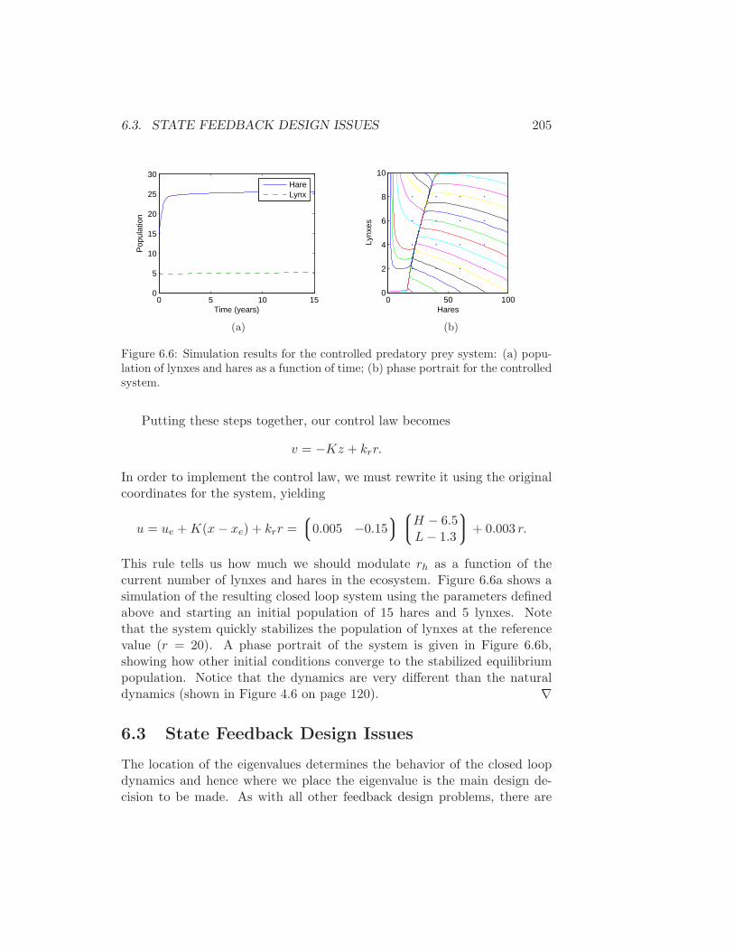
Figure 6.6: Simulation results for the controlled predatory prey system: (a) popu-lation of lynxes and hares as a function of time; (b) phase portrait for the controlledsystem.
Putting these steps together, our control law becomes
v = −Kz + krr.
In order to implement the control law, we must rewrite it using the originalcoordinates for the system, yielding
u = ue + K(x − xe) + krr =
0.005 −0.15
H − 6.5L − 1.3
+ 0.003 r.
This rule tells us how much we should modulate rh as a function of thecurrent number of lynxes and hares in the ecosystem. Figure 6.6a shows asimulation of the resulting closed loop system using the parameters definedabove and starting an initial population of 15 hares and 5 lynxes. Notethat the system quickly stabilizes the population of lynxes at the referencevalue (r = 20). A phase portrait of the system is given in Figure 6.6b,showing how other initial conditions converge to the stabilized equilibriumpopulation. Notice that the dynamics are very different than the naturaldynamics (shown in Figure 4.6 on page 120). ∇
6.3 State Feedback Design Issues
The location of the eigenvalues determines the behavior of the closed loopdynamics and hence where we place the eigenvalue is the main design de-cision to be made. As with all other feedback design problems, there are
206 CHAPTER 6. STATE FEEDBACK
tradeoffs between the magnitude of the control inputs, the robustness ofthe system to perturbations and the closed loop performance of the system,including step response, disturbance attenuation and noise injection. Forsimple systems, there are some basic guidelines that can be used and webriefly summarize them in this section.
We start by focusing on the case of second order systems, for which theclosed loop dynamics have a characteristic polynomial of the form
λ(s) = s2 + 2ζω0s + ω20. (6.22)
Since we can solve for the step and frequency response of such a systemanalytically, we can compute the various metrics described in Sections 5.3and 5.3 in closed form and write the formulas for these metrics in terms ofζ and ω0.
As an example, consider the step response for a control system withcharacteristic polynomial (6.22). This was derived in Section 5.4 and hasthe form
y(t) =k
ω20
(
1 − e−ζω0t cos ωdt +ζ
√
1 − ζ2e−ζω0t sinωdt
)
ζ < 1
y(t) =k
ω20
(
1 − eω0t − ω0t)
ζ = 1
y(t) =k
ω20
(
1 − e−ω0t − 1
2(1 + ζ)eω0(1−2ζ)t
)
ζ ≥ 1.
We focus on the case of 0 < ζ < 1 and leave the other cases as an exercisefor the reader.
To compute the maximum overshoot, we rewrite the output as
y(t) =k
ω20
(
1 − 1√
1 − ζ2e−ζω0t sin(ωdt + ϕ)
)
(6.23)
where ϕ = arccos ζ. The maximum overshoot will occur at the first time inwhich the derivative of y is zero, and hence we look for the time tp at which
0 =k
ω20
(
ζω0√
1 − ζ2e−ζω0t sin(ωdt + ϕ) − ωd
√
1 − ζ2e−ζω0t cos(ωdt + ϕ)
)
.
(6.24)Eliminating the common factors, we are left with
tan(ωdtp + ϕ) =
√
1 − ζ2
ζ.
6.3. STATE FEEDBACK DESIGN ISSUES 207
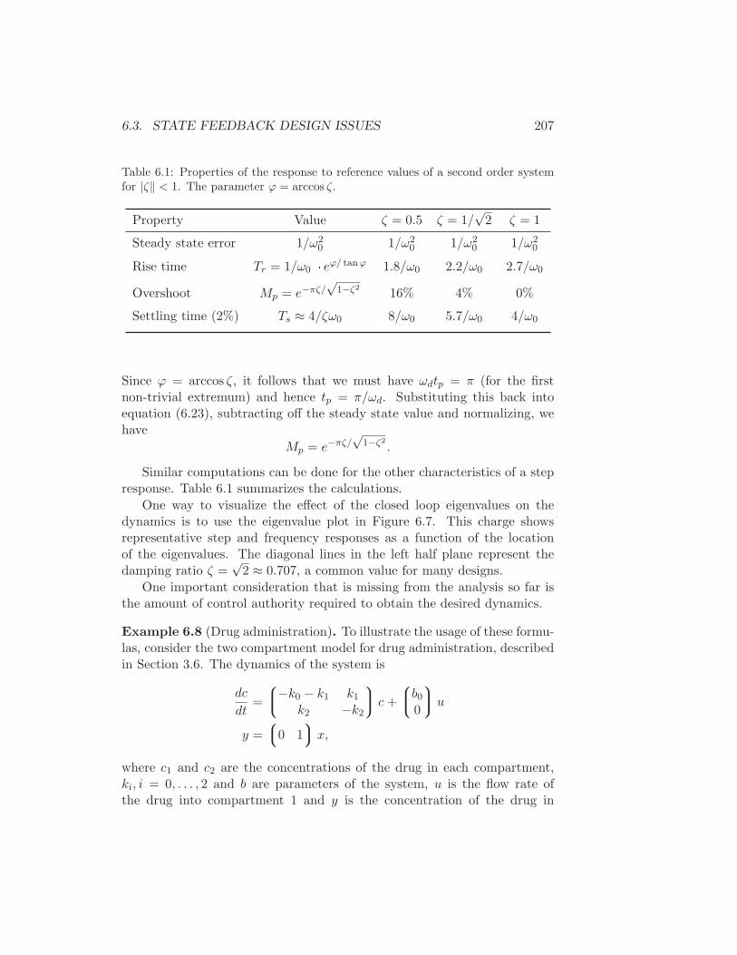
Table 6.1: Properties of the response to reference values of a second order systemfor |ζ‖ < 1. The parameter ϕ = arccos ζ.
Property Value ζ = 0.5 ζ = 1/√
2 ζ = 1
Steady state error 1/ω20 1/ω2
0 1/ω20 1/ω2
0
Rise time Tr = 1/ω0 · eϕ/ tan ϕ 1.8/ω0 2.2/ω0 2.7/ω0
Overshoot Mp = e−πζ/√
1−ζ2
16% 4% 0%
Settling time (2%) Ts ≈ 4/ζω0 8/ω0 5.7/ω0 4/ω0
Since ϕ = arccos ζ, it follows that we must have ωdtp = π (for the firstnon-trivial extremum) and hence tp = π/ωd. Substituting this back intoequation (6.23), subtracting off the steady state value and normalizing, wehave
Mp = e−πζ/√
1−ζ2
.
Similar computations can be done for the other characteristics of a stepresponse. Table 6.1 summarizes the calculations.
One way to visualize the effect of the closed loop eigenvalues on thedynamics is to use the eigenvalue plot in Figure 6.7. This charge showsrepresentative step and frequency responses as a function of the locationof the eigenvalues. The diagonal lines in the left half plane represent thedamping ratio ζ =
√2 ≈ 0.707, a common value for many designs.
One important consideration that is missing from the analysis so far isthe amount of control authority required to obtain the desired dynamics.
Example 6.8 (Drug administration). To illustrate the usage of these formu-las, consider the two compartment model for drug administration, describedin Section 3.6. The dynamics of the system is
dc
dt=
−k0 − k1 k1
k2 −k2
c +
b0
0
u
y =
0 1
x,
where c1 and c2 are the concentrations of the drug in each compartment,ki, i = 0, . . . , 2 and b are parameters of the system, u is the flow rate ofthe drug into compartment 1 and y is the concentration of the drug in
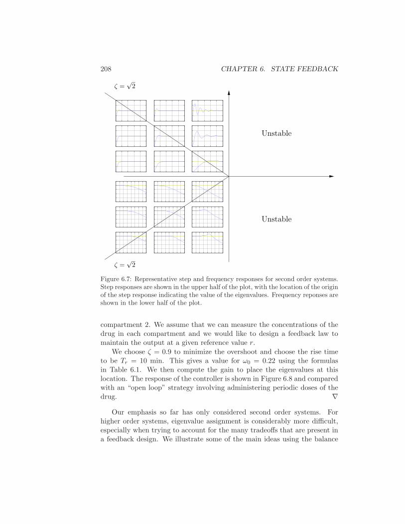
208 CHAPTER 6. STATE FEEDBACK
Unstable
Unstable
ζ =√
2
ζ =√
2
Figure 6.7: Representative step and frequency responses for second order systems.Step responses are shown in the upper half of the plot, with the location of the originof the step response indicating the value of the eigenvalues. Frequency reponses areshown in the lower half of the plot.
compartment 2. We assume that we can measure the concentrations of thedrug in each compartment and we would like to design a feedback law tomaintain the output at a given reference value r.
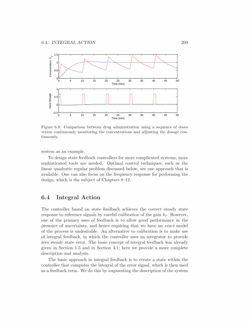
We choose ζ = 0.9 to minimize the overshoot and choose the rise timeto be Tr = 10 min. This gives a value for ω0 = 0.22 using the formulasin Table 6.1. We then compute the gain to place the eigenvalues at thislocation. The response of the controller is shown in Figure 6.8 and comparedwith an “open loop” strategy involving administering periodic doses of thedrug. ∇
Our emphasis so far has only considered second order systems. Forhigher order systems, eigenvalue assignment is considerably more difficult,especially when trying to account for the many tradeoffs that are present ina feedback design. We illustrate some of the main ideas using the balance
6.4. INTEGRAL ACTION 209
0 5 10 15 20 25 30 35 40 45 500
0.5
1
1.5
Time (min)
Con
cent
ratio
n, C
2
0 5 10 15 20 25 30 35 40 45 50−0.5
0
0.5
1
Time (min)
Inpu
t dos
age
Figure 6.8: Comparison between drug administration using a sequence of dosesversus continuously monitoring the concentrations and adjusting the dosage con-tinuously.
system as an example.
To design state feedback controllers for more complicated systems, moresophisticated tools are needed. Optimal control techniques, such as thelinear quadratic regular problem discussed below, are one approach that isavailable. One can also focus on the frequency response for performing thedesign, which is the subject of Chapters 8–12.
6.4 Integral Action
The controller based on state feedback achieves the correct steady stateresponse to reference signals by careful calibration of the gain kr. However,one of the primary uses of feedback is to allow good performance in thepresence of uncertainty, and hence requiring that we have an exact modelof the process is undesirable. An alternative to calibration is to make useof integral feedback, in which the controller uses an integrator to providezero steady state error. The basic concept of integral feedback was alreadygiven in Section 1.5 and in Section 3.1; here we provide a more completedescription and analysis.
The basic approach in integral feedback is to create a state within thecontroller that computes the integral of the error signal, which is then usedas a feedback term. We do this by augmenting the description of the system
210 CHAPTER 6. STATE FEEDBACK
with a new state z:
d
dt
xz
=
Ax + Buy − r
=
Ax + BuCx − r
The state z is seen to be the integral of the error between the desired out-put, r, and the actual output, y. Note that if we find a compensator thatstabilizes the system then necessarily we will have z = 0 in steady state andhence y = r in steady state.
Given the augmented system, we design a state space controller in theusual fashion, with a control law of the form
u = −Kx − kiz + krr
where K is the usual state feedback term, ki is the integral term and kr isused to set the nominal input for the desired steady state. The resultingequilibrium point for the system is given as
xe = −(A − BK)−1B(krr − kize)
Note that the value of ze is not specified, but rather will automatically settleto the value that makes z = y − r = 0, which implies that at equilibriumthe output will equal the reference value. This holds independently of thespecific values of A, B and K, as long as the system is stable (which can bedone through appropriate choice of K and ki).
The final compensator is given by
u = −Kx − kiz + krr
z = y − r,
where we have now included the dynamics of the integrator as part of thespecification of the controller. This type of compensator is known as adynamic compensator since it has its own internal dynamics. The followingexample illustrates the basic approach.
Example 6.9 (Cruise control). Consider the speed control example intro-duced in Section 3.1 and considered further in Example 5.10.
The linearized dynamics of the process around an equilibrium point ve,ue are given by
˙v = av − bggθ + bu
y = v = v + ve,
6.4. INTEGRAL ACTION 211
where v = v − ve, u = u− ue, m is the mass of the car and θ is the angle ofthe road. The constant a depends on the throttle characteristic and is givenin Example 5.10.
If we augment the system with an integrator, the process dynamics be-come
˙v = av − gθ + bu
z = r − y = (r − ve) − v,
or, in state space form,
d
dt
vz
=
a 0−1 0
vz
+
b0
u +
−g0
θ +
0r − ve
.
Note that when the system is at equilibrium we have that z = 0 whichimplies that the vehicle speed, v = ve + v, should be equal to the desiredreference speed, r. Our controller will be of the form
z = r − y
u = −kpv − kiz + krr
and the gains kp, ki and kr will be chosen to stabilize the system and providethe correct input for the reference speed.
Assume that we wish to design the closed loop system to have charac-teristic polynomial
λ(s) = s2 + a1s + a2.
Setting the disturbance θ = 0, the characteristic polynomial of the closedloop system is given by
det(
sI − (A − BK))
= s2 + (bK − a)s − bki
and hence we set
K =a1 + a
bki = −a2
b.
The resulting controller stabilizes the system and hence brings z = y − r tozero, resulting in perfect tracking. Notice that even if we have a small errorin the values of the parameters defining the system, as long as the closedloop poles are still stable then the tracking error will approach zero. Thusthe exact calibration required in our previous approach (using kr) is notrequired. Indeed, we can even choose kr = 0 and let the feedback controllerdo all of the work (Exercise 5).
Integral feedback can also be used to compensate for constant distur-bances. Suppose that we choose θ 6= 0, corresponding to climbing a (lin-earized) hill. The stability of the system is not affected by this external
212 CHAPTER 6. STATE FEEDBACK
disturbance and so we once again see that the car’s velocity converges tothe reference speed.
This ability to handle constant disturbances is a general property ofcontrollers with integral feedback and is explored in more detail in Exercise 6.
∇
6.5 Linear Quadratic Regulators�
In addition to selecting the closed loop eigenvalue locations to accomplish acertain objective, another way that the gains for a state feedback controllercan be chosen is by attempting to optimize a cost function.
The infinite horizon, linear quadratic regulator (LQR) problem is oneof the most common optimal control problems. Given a multi-input linearsystem
x = Ax + Bu x ∈ Rn, u ∈ R
m,
we attempt to minimize the quadratic cost function
J =
∫
∞
0
(
xT Qxx + uT Quu)
dt
where Qx ≥ 0 and Qu > 0 are symmetric, positive (semi-) definite matricesof the appropriate dimension. This cost function represents a tradeoff be-tween the distance of the state from the origin and the cost of the controlinput. By choosing the matrices Qx and Qu, described in more detail below,we can balance the rate of convergence of the solutions with the cost of thecontrol.
The solution to the LQR problem is given by a linear control law of theform
u = −Q−1u BT Px
where P ∈ Rn×n is a positive definite, symmetric matrix that satisfies the
equationPA + AT P − PBQ−1
u BT P + Qx = 0. (6.25)
Equation (6.25) is called the algebraic Riccati equation and can be solvednumerically (for example, using the lqr command in MATLAB).
One of the key questions in LQR design is how to choose the weights Qx
and Qu. In order to guarantee that a solution exists, we must have Qx ≥ 0and Qu > 0. In addition, there are certain “observability” conditions on Qx
that limit its choice. We assume here Qx > 0 to insure that solutions to thealgebraic Riccati equation always exists.
6.6. FURTHER READING 213
To choose specific values for the cost function weights Qx and Qu, wemust use our knowledge of the system we are trying to control. A particu-larly simple choice of weights is to use diagonal weights
Qx =
q1 0 · · ·. . .
0 · · · qn
Qu = ρ
r1 0 · · ·. . .
· · · 0 rn
.
For this choice of Qx and Qu, the individual diagonal elements describe howmuch each state and input (squared) should contribute to the overall cost.Hence, we can take states that should remain very small and attach higherweight values to them. Similarly, we can penalize an input versus the statesand other inputs through choice of the corresponding input weight.
6.6 Further Reading
The importance of state models and state feedback was discussed in theseminal paper by Kalman [Kal60] where the state feedback gain was obtainedby solving an optimization problem that minimized a quadratic loss function.The notions of reachability and observability (next chapter) are also due toKalman [Kal61b];see also [Gil63, KHN63]. We note that in most textbooksthe term “controllability” is used instead of “reachability”, but we preferthe latter term because it is more descriptive of the fundamental propertyof being able to reach arbitrary states.
Most undergraduate textbooks on control will contain material on statespace systems, including, for example, Franklin, Powell and Emami-Naeini [FPEN05]and Ogata [Oga01]. Friedland’s textbook [Fri04] covers the material in theprevious, current and next chapter in considerable detail, including the topicof optimal control.
6.7 Exercises
1. Consider the system shown in Figure 6.3. Write the dynamics of thetwo systems as
dx
dt= Ax + Bu
dz
dt= Az + Bu.
214 CHAPTER 6. STATE FEEDBACK
Observe that if x and z have the same initial condition, they willalways have the same state, regardless of the input that is applied.Show that this violates the definition of reachability and further showthat the reachability matrix Wr is not full rank.
2. Show that the characteristic polynomial for a system in reachablecanonical form is given by equation (6.7).
3. Consider a system on reachable canonical form. Show that the inverseof the reachability matrix is given by
W−1r =
1 a1 a2 · · · an
0 1 a1 · · · an−1...0 0 0 · · · 1
(6.26)
4. Extend the argument in Section 6.1 to show that if a system is reach-able from an initial state of zero, it is reachable from a non-zero initialstate.
5. Build a simulation for the speed controller designed in Example 6.9and show that with kr = 0, the system still achieves zero steady stateerror.
6. Show that integral feedback can be used to compensate for a constantdisturbance by giving zero steady state error even when d 6= 0.
7. Show that if y(t) is the output of a linear system corresponding toinput u(t), then the output corresponding to an input u(t) is given byy(t). (Hint: use the definition of the derivative: y(t) = limǫ→0
(
y(t +ǫ) − y(t)
)
/ǫ.)