Feedback Systems

An Introduction for Scientists and Engineers

SECOND EDITION

Karl Johan AstromRichard M. Murray

Version v3.0h (4 Sep 2016)

This is the electronic edition of Feedback Systems and is availablefrom http://www.cds.caltech.edu/∼murray/FBS. Hardcover editionsmay be purchased from Princeton University Press,http://press.princeton.edu/titles/8701.html.

This manuscript is for personal use only and may not bereproduced, in whole or in part, without written consent from thepublisher (see http://press.princeton.edu/permissions.html).

PRINCETON UNIVERSITY PRESS

PRINCETON AND OXFORD

Chapter OneIntroduction

Feedback is a central feature of life. The process of feedback governs how we grow, respond

to stress and challenge, and regulate factors such as body temperature, blood pressure and

cholesterol level. The mechanisms operate at every level, from the interaction of proteins in

cells to the interaction of organisms in complex ecologies.

M. B. Hoagland and B. Dodson, The Way Life Works, 1995 [HD95].

In this chapter we provide an introduction to the basic concept of feedbackand the related engineering discipline of control. We focus on both historical andcurrent examples, with the intention of providing the context for current tools infeedback and control.

1.1 What Is Feedback?

A dynamical system is a system whose behavior changes over time, often in re-sponse to external stimulation or forcing. The term feedback refers to a situationin which two (or more) dynamical systems are connected together such that eachsystem influences the other and their dynamics are thus strongly coupled. Simplecausal reasoning about a feedback system is difficult because the first system in-fluences the second and the second system influences the first, leading to a circularargument. A consequence of this is that the behavior of feedback systems is of-ten counter-intuitive, and it is therefore necessary to resort to formal methods tounderstand them.

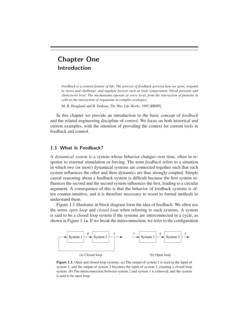
Figure 1.1 illustrates in block diagram form the idea of feedback. We often usethe terms open loop and closed loop when referring to such systems. A systemis said to be a closed loop system if the systems are interconnected in a cycle, asshown in Figure 1.1a. If we break the interconnection, we refer to the configuration

uSystem 2System 1

y

(a) Closed loop

ySystem 2System 1

ur

(b) Open loop

Figure 1.1: Open and closed loop systems. (a) The output of system 1 is used as the input ofsystem 2, and the output of system 2 becomes the input of system 1, creating a closed loopsystem. (b) The interconnection between system 2 and system 1 is removed, and the systemis said to be open loop.

1-2 CHAPTER 1. INTRODUCTION

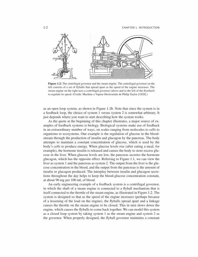
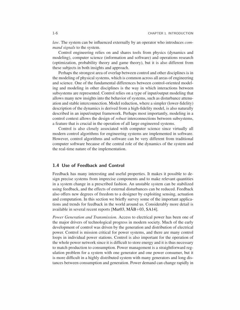
Figure 1.2: The centrifugal governor and the steam engine. The centrifugal governor on theleft consists of a set of flyballs that spread apart as the speed of the engine increases. Thesteam engine on the right uses a centrifugal governor (above and to the left of the flywheel)to regulate its speed. (Credit: Machine a Vapeur Horizontale de Philip Taylor [1828].)

as an open loop system, as shown in Figure 1.1b. Note that since the system is ina feedback loop, the choice of system 1 versus system 2 is somewhat arbitrary. Itjust depends where you want to start describing how the system works.

As the quote at the beginning of this chapter illustrates, a major source of ex-amples of feedback systems is biology. Biological systems make use of feedbackin an extraordinary number of ways, on scales ranging from molecules to cells toorganisms to ecosystems. One example is the regulation of glucose in the blood-stream through the production of insulin and glucagon by the pancreas. The bodyattempts to maintain a constant concentration of glucose, which is used by thebody’s cells to produce energy. When glucose levels rise (after eating a meal, forexample), the hormone insulin is released and causes the body to store excess glu-cose in the liver. When glucose levels are low, the pancreas secretes the hormoneglucagon, which has the opposite effect. Referring to Figure 1.1, we can view theliver as system 1 and the pancreas as system 2. The output from the liver is the glu-cose concentration in the blood, and the output from the pancreas is the amount ofinsulin or glucagon produced. The interplay between insulin and glucagon secre-tions throughout the day helps to keep the blood-glucose concentration constant,at about 90 mg per 100 mL of blood.

An early engineering example of a feedback system is a centrifugal governor,in which the shaft of a steam engine is connected to a flyball mechanism that isitself connected to the throttle of the steam engine, as illustrated in Figure 1.2. Thesystem is designed so that as the speed of the engine increases (perhaps becauseof a lessening of the load on the engine), the flyballs spread apart and a linkagecauses the throttle on the steam engine to be closed. This in turn slows down theengine, which causes the flyballs to come back together. We can model this systemas a closed loop system by taking system 1 as the steam engine and system 2 asthe governor. When properly designed, the flyball governor maintains a constant

1.1. WHAT IS FEEDBACK? 1-3

speed of the engine, roughly independent of the loading conditions. The centrifugalgovernor was an enabler of the successful Watt steam engine, which fueled theindustrial revolution.

The examples given so far all deal with negative feedback, in which we attemptto react to disturbances in a such a way that their effects decrease. Positive feedbackis the opposite, where the increase in some variable or signal leads to a situationin which that quantity is further increased through feedback. This has a destabi-lizing effect and is usually accompanied by a saturation that limits the growth ofthe quantity. Although often considered undesirable, this behavior is used in bio-logical (and engineering) systems to obtain a very fast response to a condition orsignal. Encouragement is a positive feedback that is often used in education. An-other common use of positive feedback is the design of systems with oscillatorydynamics.

One example of the use of positive feedback is to create switching behavior,in which a system maintains a given state until some input crosses a threshold.Hysteresis is often present so that noisy inputs near the threshold do not cause thesystem to jitter. This type of behavior is called bistability and is often associatedwith memory devices.

Feedback has many interesting properties that can be exploited in designingsystems. As in the case of glucose regulation or the flyball governor, feedback canmake a system resilient toward external influences. It can also be used to createlinear behavior out of nonlinear components, a common approach in electronics.More generally, feedback allows a system to be insensitive both to external distur-bances and to variations in its individual elements.

Feedback has potential disadvantages as well. It can create dynamic instabili-ties in a system, causing oscillations or even runaway behavior. Another drawback,especially in engineering systems, is that feedback can introduce unwanted sensornoise into the system, requiring careful filtering of signals. It is for these reasonsthat a substantial portion of the study of feedback systems is devoted to developingan understanding of dynamics and a mastery of techniques in dynamical systems.

Feedback systems are ubiquitous in both natural and engineered systems. Con-trol systems maintain the environment, lighting and power in our buildings andfactories; they regulate the operation of our cars, consumer electronics and manu-facturing processes; they enable our transportation and communications systems;and they are critical elements in our military and space systems. For the most partthey are hidden from view, buried within the code of embedded microprocessors,executing their functions accurately and reliably. Feedback has also made it pos-sible to increase dramatically the precision of instruments such as atomic forcemicroscopes (AFMs) and telescopes.

In nature, homeostasis in biological systems maintains thermal, chemical andbiological conditions through feedback. At the other end of the size scale, globalclimate dynamics depend on the feedback interactions between the atmosphere,the oceans, the land and the sun. Ecosystems are filled with examples of feedbackdue to the complex interactions between animal and plant life. Even the dynam-

1-4 CHAPTER 1. INTRODUCTION

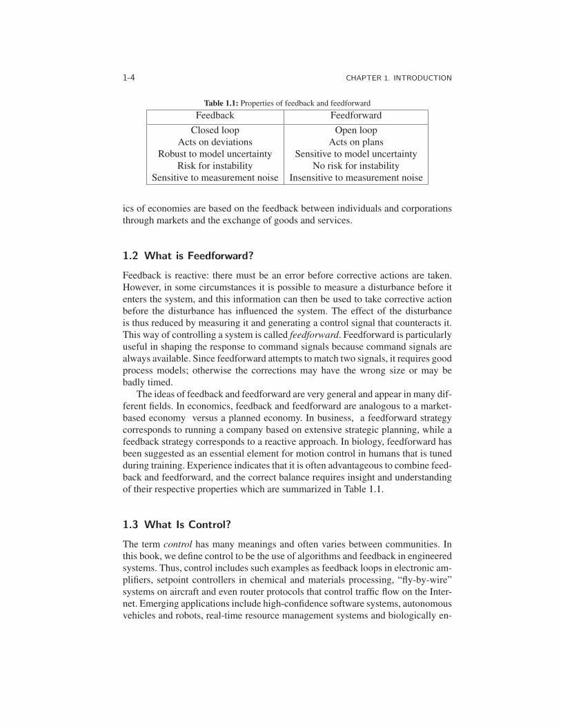
Table 1.1: Properties of feedback and feedforward

Feedback Feedforward

Closed loop Open loopActs on deviations Acts on plans

Robust to model uncertainty Sensitive to model uncertaintyRisk for instability No risk for instability

Sensitive to measurement noise Insensitive to measurement noise

ics of economies are based on the feedback between individuals and corporationsthrough markets and the exchange of goods and services.

1.2 What is Feedforward?

Feedback is reactive: there must be an error before corrective actions are taken.However, in some circumstances it is possible to measure a disturbance before itenters the system, and this information can then be used to take corrective actionbefore the disturbance has influenced the system. The effect of the disturbanceis thus reduced by measuring it and generating a control signal that counteracts it.This way of controlling a system is called feedforward. Feedforward is particularlyuseful in shaping the response to command signals because command signals arealways available. Since feedforward attempts to match two signals, it requires goodprocess models; otherwise the corrections may have the wrong size or may bebadly timed.

The ideas of feedback and feedforward are very general and appear in many dif-ferent fields. In economics, feedback and feedforward are analogous to a market-based economy versus a planned economy. In business, a feedforward strategycorresponds to running a company based on extensive strategic planning, while afeedback strategy corresponds to a reactive approach. In biology, feedforward hasbeen suggested as an essential element for motion control in humans that is tunedduring training. Experience indicates that it is often advantageous to combine feed-back and feedforward, and the correct balance requires insight and understandingof their respective properties which are summarized in Table 1.1.

1.3 What Is Control?

The term control has many meanings and often varies between communities. Inthis book, we define control to be the use of algorithms and feedback in engineeredsystems. Thus, control includes such examples as feedback loops in electronic am-plifiers, setpoint controllers in chemical and materials processing, “fly-by-wire”systems on aircraft and even router protocols that control traffic flow on the Inter-net. Emerging applications include high-confidence software systems, autonomousvehicles and robots, real-time resource management systems and biologically en-

1.3. WHAT IS CONTROL? 1-5

Controller

System Sensors

Filter

Clock

operator input

D/A Computer A/D

noiseexternal disturbancesnoise

ΣΣOutput

Process

Actuators

Figure 1.3: Components of a computer-controlled system. The upper dashed box representsthe process dynamics, which include the sensors and actuators in addition to the dynamicalsystem being controlled. Noise and external disturbances can perturb the dynamics of theprocess. The controller is shown in the lower dashed box. It consists of a filter and analog-to-digital (A/D) and digital-to-analog (D/A) converters, as well as a computer that implementsthe control algorithm. A system clock controls the operation of the controller, synchronizingthe A/D, D/A and computing processes. The operator input is also fed to the computer as anexternal input.

gineered systems. At its core, control is an information science and includes theuse of information in both analog and digital representations.

A modern controller senses the operation of a system, compares it against thedesired behavior, computes corrective actions based on a model of the system’sresponse to external inputs and actuates the system to effect the desired change.This basic feedback loop of sensing, computation and actuation is the central con-cept in control. The key issues in designing control logic are ensuring that the dy-namics of the closed loop system are stable (bounded disturbances give boundederrors) and that they have additional desired behavior (good disturbance attenua-tion, fast responsiveness to changes in operating point, etc). These properties areestablished using a variety of modeling and analysis techniques that capture theessential dynamics of the system and permit the exploration of possible behaviorsin the presence of uncertainty, noise and component failure.

A typical example of a control system is shown in Figure 1.3. The basic ele-ments of sensing, computation and actuation are clearly seen. In modern controlsystems, computation is typically implemented on a digital computer, requiring theuse of analog-to-digital (A/D) and digital-to-analog (D/A) converters. Uncertaintyenters the system through noise in sensing and actuation subsystems, external dis-turbances that affect the underlying system operation and uncertain dynamics inthe system (parameter errors, unmodeled effects, etc). The algorithm that com-putes the control action as a function of the sensor values is often called a control

1-6 CHAPTER 1. INTRODUCTION

law. The system can be influenced externally by an operator who introduces com-mand signals to the system.

Control engineering relies on and shares tools from physics (dynamics andmodeling), computer science (information and software) and operations research(optimization, probability theory and game theory), but it is also different fromthese subjects in both insights and approach.

Perhaps the strongest area of overlap between control and other disciplines is inthe modeling of physical systems, which is common across all areas of engineeringand science. One of the fundamental differences between control-oriented model-ing and modeling in other disciplines is the way in which interactions betweensubsystems are represented. Control relies on a type of input/output modeling thatallows many new insights into the behavior of systems, such as disturbance attenu-ation and stable interconnection. Model reduction, where a simpler (lower-fidelity)description of the dynamics is derived from a high-fidelity model, is also naturallydescribed in an input/output framework. Perhaps most importantly, modeling in acontrol context allows the design of robust interconnections between subsystems,a feature that is crucial in the operation of all large engineered systems.

Control is also closely associated with computer science since virtually allmodern control algorithms for engineering systems are implemented in software.However, control algorithms and software can be very different from traditionalcomputer software because of the central role of the dynamics of the system andthe real-time nature of the implementation.

1.4 Use of Feedback and Control

Feedback has many interesting and useful properties. It makes it possible to de-sign precise systems from imprecise components and to make relevant quantitiesin a system change in a prescribed fashion. An unstable system can be stabilizedusing feedback, and the effects of external disturbances can be reduced. Feedbackalso offers new degrees of freedom to a designer by exploiting sensing, actuationand computation. In this section we briefly survey some of the important applica-tions and trends for feedback in the world around us. Considerably more detail isavailable in several recent reports [Mur03, MAB+03, SA14].

Power Generation and Transmission. Access to electrical power has been one ofthe major drivers of technological progress in modern society. Much of the earlydevelopment of control was driven by the generation and distribution of electricalpower. Control is mission critical for power systems, and there are many controlloops in individual power stations. Control is also important for the operation ofthe whole power network since it is difficult to store energy and it is thus necessaryto match production to consumption. Power management is a straightforward reg-ulation problem for a system with one generator and one power consumer, but itis more difficult in a highly distributed system with many generators and long dis-tances between consumption and generation. Power demand can change rapidly in

1.4. USE OF FEEDBACK AND CONTROL 1-7

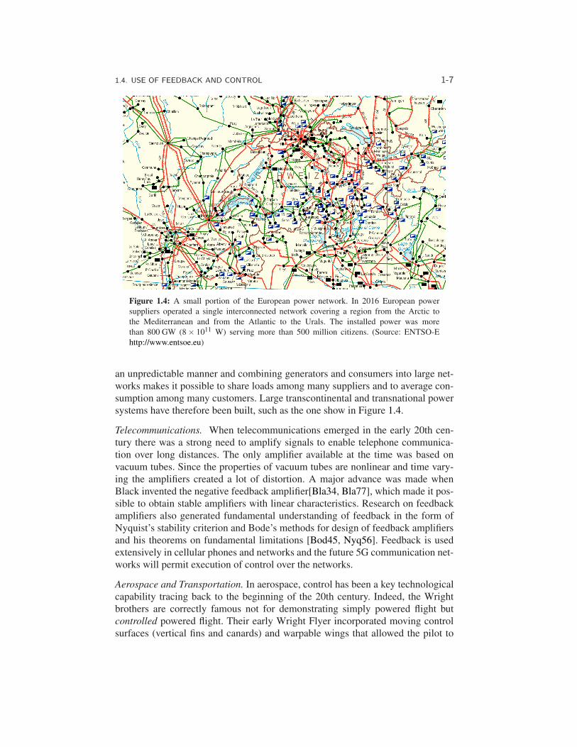
Figure 1.4: A small portion of the European power network. In 2016 European powersuppliers operated a single interconnected network covering a region from the Arctic tothe Mediterranean and from the Atlantic to the Urals. The installed power was morethan 800 GW (8× 1011 W) serving more than 500 million citizens. (Source: ENTSO-Ehttp://www.entsoe.eu)

an unpredictable manner and combining generators and consumers into large net-works makes it possible to share loads among many suppliers and to average con-sumption among many customers. Large transcontinental and transnational powersystems have therefore been built, such as the one show in Figure 1.4.

Telecommunications. When telecommunications emerged in the early 20th cen-tury there was a strong need to amplify signals to enable telephone communica-tion over long distances. The only amplifier available at the time was based onvacuum tubes. Since the properties of vacuum tubes are nonlinear and time vary-ing the amplifiers created a lot of distortion. A major advance was made whenBlack invented the negative feedback amplifier[Bla34, Bla77], which made it pos-sible to obtain stable amplifiers with linear characteristics. Research on feedbackamplifiers also generated fundamental understanding of feedback in the form ofNyquist’s stability criterion and Bode’s methods for design of feedback amplifiersand his theorems on fundamental limitations [Bod45, Nyq56]. Feedback is usedextensively in cellular phones and networks and the future 5G communication net-works will permit execution of control over the networks.

Aerospace and Transportation. In aerospace, control has been a key technologicalcapability tracing back to the beginning of the 20th century. Indeed, the Wrightbrothers are correctly famous not for demonstrating simply powered flight butcontrolled powered flight. Their early Wright Flyer incorporated moving controlsurfaces (vertical fins and canards) and warpable wings that allowed the pilot to

1-8 CHAPTER 1. INTRODUCTION

regulate the aircraft’s flight. In fact, the aircraft itself was not stable, so continuouspilot corrections were mandatory. This early example of controlled flight was fol-lowed by a fascinating success story of continuous improvements in flight controltechnology, culminating in the high-performance, highly reliable automatic flightcontrol systems we see in modern commercial and military aircraft today.

Materials and Processing. The chemical industry is responsible for the remarkableprogress in developing new materials that are key to our modern society. In addi-tion to the continuing need to improve product quality, several other factors in theprocess control industry are drivers for the use of control. Environmental statutescontinue to place stricter limitations on the production of pollutants, forcing theuse of sophisticated pollution control devices. Environmental safety considera-tions have led to the design of smaller storage capacities to diminish the risk ofmajor chemical leakage, requiring tighter control on upstream processes and, insome cases, supply chains. And large increases in energy costs have encouragedengineers to design plants that are highly integrated, coupling many processes thatused to operate independently. All of these trends increase the complexity of theseprocesses and the performance requirements for the control systems, making con-trol system design increasingly challenging.

Instrumentation. The measurement of physical variables is of prime interest inscience and engineering. Consider, for example, an accelerometer, where early in-struments consisted of a mass suspended on a spring with a deflection sensor. Theprecision of such an instrument depends critically on accurate calibration of thespring and the sensor. There is also a design compromise because a weak springgives high sensitivity but low bandwidth. A different way of measuring accelera-tion is to use force feedback. The spring is replaced by a voice coil that is controlledso that the mass remains at a constant position. The acceleration is proportional tothe current through the voice coil. In such an instrument, the precision depends en-tirely on the calibration of the voice coil and does not depend on the sensor, whichis used only as the feedback signal. The sensitivity/bandwidth compromise is alsoavoided.

Another important application of feedback is in instrumentation for biologicalsystems. Feedback is widely used to measure ion currents in cells using a devicecalled a voltage clamp, which is illustrated in Figure 1.5. Hodgkin and Huxleyused the voltage clamp to investigate propagation of action potentials in the giantaxon of the squid. In 1963 they shared the Nobel Prize in Medicine with Ecclesfor “their discoveries concerning the ionic mechanisms involved in excitation andinhibition in the peripheral and central portions of the nerve cell membrane.” Arefinement of the voltage clamp called a patch clamp made it possible to measureexactly when a single ion channel is opened or closed. This was developed byNeher and Sakmann, who received the 1991 Nobel Prize in Medicine “for theirdiscoveries concerning the function of single ion channels in cells.”

Robotics and Intelligent Machines. The goal of cybernetic engineering, already ar-ticulated in the 1940s and even before, has been to implement systems capable of

1.4. USE OF FEEDBACK AND CONTROL 1-9

Electrode

Glass Pipette

Ion Channel

Cell Membrane

ControllerI -

+

∆vr∆v

ve

vi

Figure 1.5: The voltage clamp method for measuring ion currents in cells using feedback. Apipette is used to place an electrode in a cell (left and middle) and maintain the potential ofthe cell at a fixed level. The internal voltage in the cell is vi, and the voltage of the externalfluid is ve. The feedback system (right) controls the current I into the cell so that the voltagedrop across the cell membrane ∆v = vi− ve is equal to its reference value ∆vr. The current I

is then equal to the ion current.

exhibiting highly flexible or “intelligent” responses to changing circumstances. In1948 the MIT mathematician Norbert Wiener gave a widely read account of cy-bernetics [Wie48]. A more mathematical treatment of the elements of engineeringcybernetics was presented by H. S. Tsien in 1954, driven by problems related tothe control of missiles [Tsi54]. Together, these works and others of that time formmuch of the intellectual basis for modern work in robotics and control.

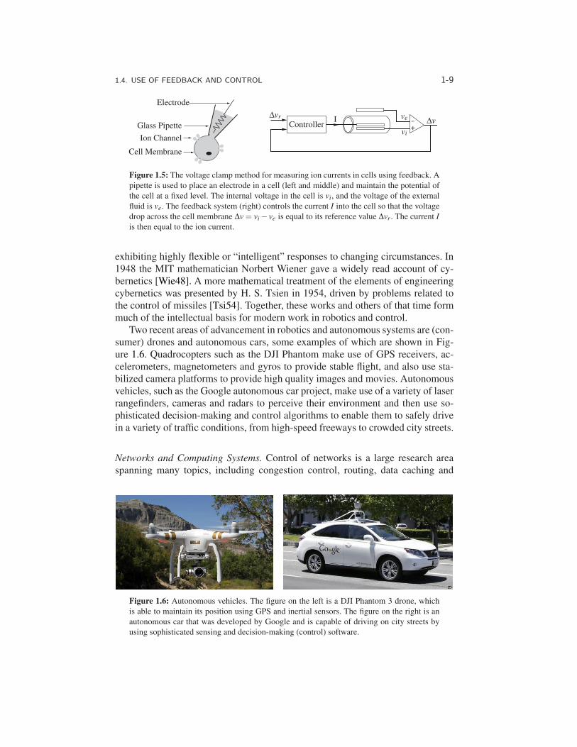
Two recent areas of advancement in robotics and autonomous systems are (con-sumer) drones and autonomous cars, some examples of which are shown in Fig-ure 1.6. Quadrocopters such as the DJI Phantom make use of GPS receivers, ac-celerometers, magnetometers and gyros to provide stable flight, and also use sta-bilized camera platforms to provide high quality images and movies. Autonomousvehicles, such as the Google autonomous car project, make use of a variety of laserrangefinders, cameras and radars to perceive their environment and then use so-phisticated decision-making and control algorithms to enable them to safely drivein a variety of traffic conditions, from high-speed freeways to crowded city streets.

Networks and Computing Systems. Control of networks is a large research areaspanning many topics, including congestion control, routing, data caching and

Figure 1.6: Autonomous vehicles. The figure on the left is a DJI Phantom 3 drone, whichis able to maintain its position using GPS and inertial sensors. The figure on the right is anautonomous car that was developed by Google and is capable of driving on city streets byusing sophisticated sensing and decision-making (control) software.

1-10 CHAPTER 1. INTRODUCTION

The Internet

Request

Reply

Request

Reply

Request

Reply

Tier 1 Tier 2 Tier 3

Clients

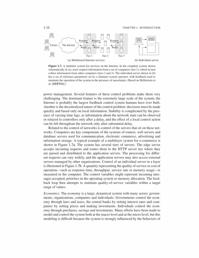
(a) Multitiered Internet services (b) Individual server

Figure 1.7: A multitier system for services on the Internet. In the complete system shownschematically in (a), users request information from a set of computers (tier 1), which in turncollect information from other computers (tiers 2 and 3). The individual server shown in (b)has a set of reference parameters set by a (human) system operator, with feedback used tomaintain the operation of the system in the presence of uncertainty. (Based on Hellerstein etal. [HDPT04].)

power management. Several features of these control problems make them verychallenging. The dominant feature is the extremely large scale of the system; theInternet is probably the largest feedback control system humans have ever built.Another is the decentralized nature of the control problem: decisions must be madequickly and based only on local information. Stability is complicated by the pres-ence of varying time lags, as information about the network state can be observedor relayed to controllers only after a delay, and the effect of a local control actioncan be felt throughout the network only after substantial delay.

Related to the control of networks is control of the servers that sit on these net-works. Computers are key components of the systems of routers, web servers anddatabase servers used for communication, electronic commerce, advertising andinformation storage. A typical example of a multilayer system for e-commerce isshown in Figure 1.7a. The system has several tiers of servers. The edge serveraccepts incoming requests and routes them to the HTTP server tier where theyare parsed and distributed to the application servers. The processing for differ-ent requests can vary widely, and the application servers may also access externalservers managed by other organizations. Control of an individual server in a layeris illustrated in Figure 1.7b. A quantity representing the quality of service or cost ofoperation—such as response time, throughput, service rate or memory usage—ismeasured in the computer. The control variables might represent incoming mes-sages accepted, priorities in the operating system or memory allocation. The feed-back loop then attempts to maintain quality-of-service variables within a targetrange of values.

Economics. The economy is a large, dynamical system with many actors: govern-ments, organizations, companies and individuals. Governments control the econ-omy through laws and taxes, the central banks by setting interest rates and com-panies by setting prices and making investments. Individuals control the econ-omy through purchases, savings and investments. Many efforts have been made tomodel and control the system both at the macro level and at the micro level, but thismodeling is difficult because the system is strongly influenced by the behaviors of

1.4. USE OF FEEDBACK AND CONTROL 1-11

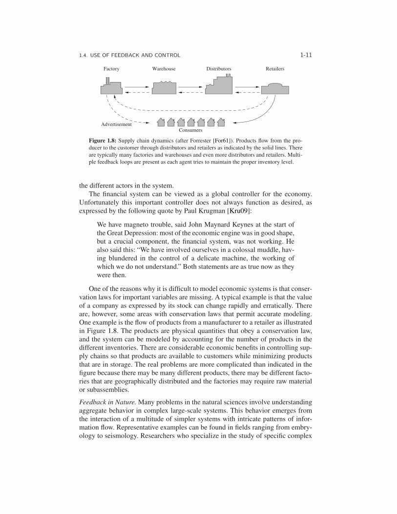
Factory Warehouse Distributors

ConsumersAdvertisement

Retailers

Figure 1.8: Supply chain dynamics (after Forrester [For61]). Products flow from the pro-ducer to the customer through distributors and retailers as indicated by the solid lines. Thereare typically many factories and warehouses and even more distributors and retailers. Multi-ple feedback loops are present as each agent tries to maintain the proper inventory level.

the different actors in the system.The financial system can be viewed as a global controller for the economy.

Unfortunately this important controller does not always function as desired, asexpressed by the following quote by Paul Krugman [Kru09]:

We have magneto trouble, said John Maynard Keynes at the start ofthe Great Depression: most of the economic engine was in good shape,but a crucial component, the financial system, was not working. Healso said this: “We have involved ourselves in a colossal muddle, hav-ing blundered in the control of a delicate machine, the working ofwhich we do not understand.” Both statements are as true now as theywere then.

One of the reasons why it is difficult to model economic systems is that conser-vation laws for important variables are missing. A typical example is that the valueof a company as expressed by its stock can change rapidly and erratically. Thereare, however, some areas with conservation laws that permit accurate modeling.One example is the flow of products from a manufacturer to a retailer as illustratedin Figure 1.8. The products are physical quantities that obey a conservation law,and the system can be modeled by accounting for the number of products in thedifferent inventories. There are considerable economic benefits in controlling sup-ply chains so that products are available to customers while minimizing productsthat are in storage. The real problems are more complicated than indicated in thefigure because there may be many different products, there may be different facto-ries that are geographically distributed and the factories may require raw materialor subassemblies.

Feedback in Nature. Many problems in the natural sciences involve understandingaggregate behavior in complex large-scale systems. This behavior emerges fromthe interaction of a multitude of simpler systems with intricate patterns of infor-mation flow. Representative examples can be found in fields ranging from embry-ology to seismology. Researchers who specialize in the study of specific complex

1-12 CHAPTER 1. INTRODUCTION

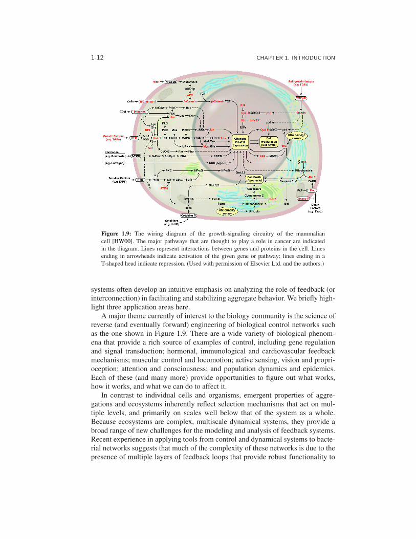
Figure 1.9: The wiring diagram of the growth-signaling circuitry of the mammaliancell [HW00]. The major pathways that are thought to play a role in cancer are indicatedin the diagram. Lines represent interactions between genes and proteins in the cell. Linesending in arrowheads indicate activation of the given gene or pathway; lines ending in aT-shaped head indicate repression. (Used with permission of Elsevier Ltd. and the authors.)

systems often develop an intuitive emphasis on analyzing the role of feedback (orinterconnection) in facilitating and stabilizing aggregate behavior. We briefly high-light three application areas here.

A major theme currently of interest to the biology community is the science ofreverse (and eventually forward) engineering of biological control networks suchas the one shown in Figure 1.9. There are a wide variety of biological phenom-ena that provide a rich source of examples of control, including gene regulationand signal transduction; hormonal, immunological and cardiovascular feedbackmechanisms; muscular control and locomotion; active sensing, vision and propri-oception; attention and consciousness; and population dynamics and epidemics.Each of these (and many more) provide opportunities to figure out what works,how it works, and what we can do to affect it.

In contrast to individual cells and organisms, emergent properties of aggre-gations and ecosystems inherently reflect selection mechanisms that act on mul-tiple levels, and primarily on scales well below that of the system as a whole.Because ecosystems are complex, multiscale dynamical systems, they provide abroad range of new challenges for the modeling and analysis of feedback systems.Recent experience in applying tools from control and dynamical systems to bacte-rial networks suggests that much of the complexity of these networks is due to thepresence of multiple layers of feedback loops that provide robust functionality to

1.5. FEEDBACK PROPERTIES 1-13

the individual cell [Kit04, SSS+04, YHSD00a]. Yet in other instances, events atthe cell level benefit the colony at the expense of the individual. Systems level anal-ysis can be applied to ecosystems with the goal of understanding the robustness ofsuch systems and the extent to which decisions and events affecting individualspecies contribute to the robustness and/or fragility of the ecosystem as a whole.

In nature, development of organisms and their control systems have often de-veloped in synergy. The development of birds is an interesting example, as notedby John Maynard Smith in 1952 [Smi52b]:

The earliest birds pterosaurs, and flying insects were stable. This isbelieved to be because in the absence of a highly evolved sensory andnervous system they would have been unable to fly if they were not. Toa flying animal there are great advantages to be gained by instability.Among the most obvious is manoeuvrability. It is of equal importanceto an animal which catches its food in the air and to the animals uponwhich it preys. It appears that in the birds and at least in some insectsthe evolution of the sensory and nervous systems rendered the stabilityfound in earlier forms no longer necessary.

1.5 Feedback Properties

Feedback is a powerful idea which, as we have seen, is used extensively in naturaland technological systems. The principle of feedback is simple: base correctingactions on the difference between desired and actual performance. In engineering,feedback has been rediscovered and patented many times in many different con-texts. The use of feedback has often resulted in vast improvements in system ca-pability, and these improvements have sometimes been revolutionary, as discussedabove. The reason for this is that feedback has some truly remarkable properties.In this section we will discuss some of the properties of feedback that can be un-derstood intuitively. This intuition will be formalized in subsequent chapters.

Robustness to Uncertainty

One of the key uses of feedback is to provide robustness to uncertainty. By mea-suring the difference between the sensed value of a regulated signal and its desiredvalue, we can supply a corrective action. If the system undergoes some change thataffects the regulated signal, then we sense this change and try to force the systemback to the desired operating point. This is precisely the effect that Watt exploitedin his use of the centrifugal governor on steam engines.

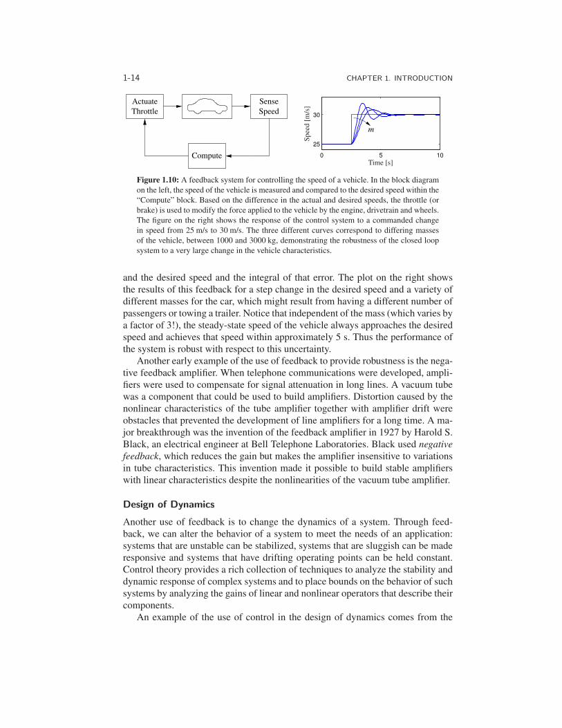
As an example of this principle, consider the simple feedback system shown inFigure 1.10. In this system, the speed of a vehicle is controlled by adjusting theamount of gas flowing to the engine. Simple proportional-integral (PI) feedbackis used to make the amount of gas depend on both the error between the current

1-14 CHAPTER 1. INTRODUCTION

Compute

ActuateThrottle

SenseSpeed

0 5 10

25

30

Spe

ed[m

/s]

Time [s]

m

Figure 1.10: A feedback system for controlling the speed of a vehicle. In the block diagramon the left, the speed of the vehicle is measured and compared to the desired speed within the“Compute” block. Based on the difference in the actual and desired speeds, the throttle (orbrake) is used to modify the force applied to the vehicle by the engine, drivetrain and wheels.The figure on the right shows the response of the control system to a commanded changein speed from 25 m/s to 30 m/s. The three different curves correspond to differing massesof the vehicle, between 1000 and 3000 kg, demonstrating the robustness of the closed loopsystem to a very large change in the vehicle characteristics.

and the desired speed and the integral of that error. The plot on the right showsthe results of this feedback for a step change in the desired speed and a variety ofdifferent masses for the car, which might result from having a different number ofpassengers or towing a trailer. Notice that independent of the mass (which varies bya factor of 3!), the steady-state speed of the vehicle always approaches the desiredspeed and achieves that speed within approximately 5 s. Thus the performance ofthe system is robust with respect to this uncertainty.

Another early example of the use of feedback to provide robustness is the nega-tive feedback amplifier. When telephone communications were developed, ampli-fiers were used to compensate for signal attenuation in long lines. A vacuum tubewas a component that could be used to build amplifiers. Distortion caused by thenonlinear characteristics of the tube amplifier together with amplifier drift wereobstacles that prevented the development of line amplifiers for a long time. A ma-jor breakthrough was the invention of the feedback amplifier in 1927 by Harold S.Black, an electrical engineer at Bell Telephone Laboratories. Black used negativefeedback, which reduces the gain but makes the amplifier insensitive to variationsin tube characteristics. This invention made it possible to build stable amplifierswith linear characteristics despite the nonlinearities of the vacuum tube amplifier.

Design of Dynamics

Another use of feedback is to change the dynamics of a system. Through feed-back, we can alter the behavior of a system to meet the needs of an application:systems that are unstable can be stabilized, systems that are sluggish can be maderesponsive and systems that have drifting operating points can be held constant.Control theory provides a rich collection of techniques to analyze the stability anddynamic response of complex systems and to place bounds on the behavior of suchsystems by analyzing the gains of linear and nonlinear operators that describe theircomponents.

An example of the use of control in the design of dynamics comes from the

1.5. FEEDBACK PROPERTIES 1-15

area of flight control. The following quote, from a lecture presented by WilburWright to the Western Society of Engineers in 1901 [McF53], illustrates the roleof control in the development of the airplane:

Men already know how to construct wings or airplanes, which whendriven through the air at sufficient speed, will not only sustain theweight of the wings themselves, but also that of the engine, and ofthe engineer as well. Men also know how to build engines and screwsof sufficient lightness and power to drive these planes at sustainingspeed ... Inability to balance and steer still confronts students of theflying problem ... When this one feature has been worked out, theage of flying will have arrived, for all other difficulties are of minorimportance.

The Wright brothers thus realized that control was a key issue to enable flight.They resolved the compromise between stability and maneuverability by buildingan airplane, the Wright Flyer, that was unstable but maneuverable. The Flyer hada rudder in the front of the airplane, which made the plane very maneuverable. Adisadvantage was the necessity for the pilot to keep adjusting the rudder to fly theplane: if the pilot let go of the stick, the plane would crash. Other early aviatorstried to build stable airplanes. These would have been easier to fly, but because oftheir poor maneuverability they could not be brought up into the air. The WrightBrothers were well aware of the compromise between stability and maneuverabil-ity when the designed they Wright Flyer [Dra55] and they made the first successfulflight at Kitty Hawk in 1903. Modern fighter airplanes are also unstable in certainflight regimes, such as take-off and landing.

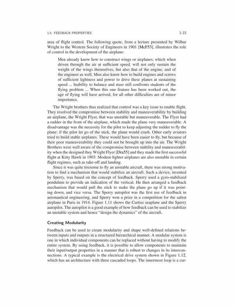
Since it was quite tiresome to fly an unstable aircraft, there was strong motiva-tion to find a mechanism that would stabilize an aircraft. Such a device, inventedby Sperry, was based on the concept of feedback. Sperry used a gyro-stabilizedpendulum to provide an indication of the vertical. He then arranged a feedbackmechanism that would pull the stick to make the plane go up if it was point-ing down, and vice versa. The Sperry autopilot was the first use of feedback inaeronautical engineering, and Sperry won a prize in a competition for the safestairplane in Paris in 1914. Figure 1.11 shows the Curtiss seaplane and the Sperryautopilot. The autopilot is a good example of how feedback can be used to stabilizean unstable system and hence “design the dynamics” of the aircraft.

Creating Modularity

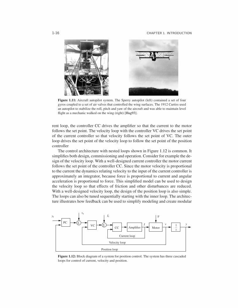
Feedback can be used to create modularity and shape well-defined relations be-tween inputs and outputs in a structured hierarchical manner. A modular system isone in which individual components can be replaced without having to modify theentire system. By using feedback, it is possible to allow components to maintaintheir input/output properties in a manner that is robust to changes in its intercon-nections. A typical example is the electrical drive system shown in Figure 1.12,which has an architecture with three cascaded loops. The innermost loop is a cur-

1-16 CHAPTER 1. INTRODUCTION

Figure 1.11: Aircraft autopilot system. The Sperry autopilot (left) contained a set of fourgyros coupled to a set of air valves that controlled the wing surfaces. The 1912 Curtiss usedan autopilot to stabilize the roll, pitch and yaw of the aircraft and was able to maintain levelflight as a mechanic walked on the wing (right) [Hug93].

rent loop, the controller CC drives the amplifier so that the current to the motorfollows the set point. The velocity loop with the controller VC drives the set pointof the current controller so that velocity follows the set point of VC. The outerloop drives the set point of the velocity loop to follow the set point of the positioncontroller

The control architecture with nested loops shown in Figure 1.12 is common. Itsimplifies both design, commissioning and operation. Consider for example the de-sign of the velocity loop. With a well-designed current controller the motor currentfollows the set point of the controller CC. Since the motor velocity is proportionalto the current the dynamics relating velocity to the input of the current controller isapproximately an integrator, because force is proportional to current and angularacceleration is proportional to force. This simplified model can be used to designthe velocity loop so that effects of friction and other disturbances are reduced.With a well-designed velocity loop, the design of the position loop is also simple.The loops can also be tuned sequentially starting with the inner loop. The architec-ture illustrates how feedback can be used to simplify modeling and create modular

yr

I v y

vrIr

ΣΣ

PCVC

CC Amplifier Motor1

s

Current loop

Velocity loop

Position loop

F

Figure 1.12: Block diagram of a system for position control. The system has three cascadedloops for control of current, velocity and position.

1.6. SIMPLE FORMS OF FEEDBACK 1-17

systems.

Challenges of Feedback

While feedback has many advantages, it also has some potential drawbacks. Chiefamong these is the possibility of instability if the system is not designed properly.We are all familiar with the effects of positive feedback when the amplificationon a microphone is turned up too high in a room. This is an example of feedbackinstability, something that we obviously want to avoid. This is tricky because wemust design the system not only to be stable under nominal conditions but also toremain stable under all possible perturbations of the dynamics.

In addition to the potential for instability, feedback inherently couples differentparts of a system. One common problem is that feedback often injects measure-ment noise into the system. Measurements must be carefully filtered so that theactuation and process dynamics do not respond to them, while at the same timeensuring that the measurement signal from the sensor is properly coupled into theclosed loop dynamics (so that the proper levels of performance are achieved).

Another potential drawback of control is the complexity of embedding a con-trol system in a product. While the cost of sensing, computation and actuation hasdecreased dramatically in the past few decades, the fact remains that control sys-tems are often complicated, and hence one must carefully balance the costs andbenefits. An early engineering example of this is the use of microprocessor-basedfeedback systems in automobiles.The use of microprocessors in automotive appli-cations began in the early 1970s and was driven by increasingly strict emissionsstandards, which could be met only through electronic controls. Early systemswere expensive and failed more often than desired, leading to frequent customerdissatisfaction. It was only through aggressive improvements in technology thatthe performance, reliability and cost of these systems allowed them to be used in atransparent fashion. Even today, the complexity of these systems is such that it isdifficult for an individual car owner to fix problems.

1.6 Simple Forms of Feedback

The idea of feedback to make corrective actions based on the difference betweenthe desired and the actual values of a quantity can be implemented in many differ-ent ways. The benefits of feedback can be obtained by very simple feedback lawssuch as on-off control, proportional control and proportional-integral-derivativecontrol. In this section we provide a brief preview of some of the topics that willbe studied more formally in the remainder of the text.

1-18 CHAPTER 1. INTRODUCTION

u

e

(a) On-off control

u

e

(b) Dead zone

u

e

(c) Hysteresis

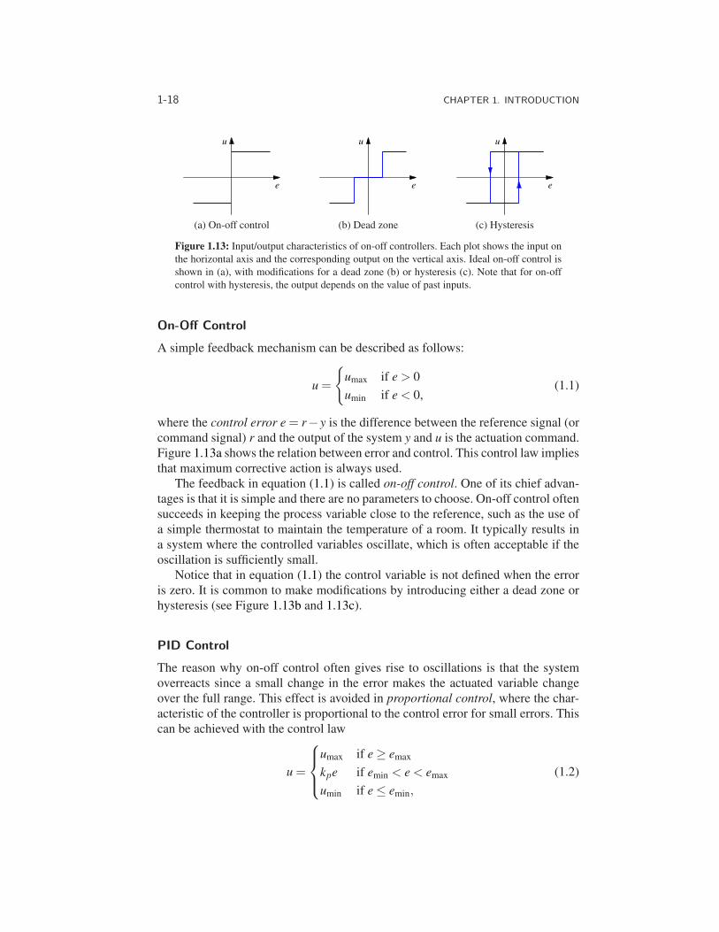
Figure 1.13: Input/output characteristics of on-off controllers. Each plot shows the input onthe horizontal axis and the corresponding output on the vertical axis. Ideal on-off control isshown in (a), with modifications for a dead zone (b) or hysteresis (c). Note that for on-offcontrol with hysteresis, the output depends on the value of past inputs.

On-Off Control

A simple feedback mechanism can be described as follows:

u =

{umax if e > 0

umin if e < 0,(1.1)

where the control error e = r−y is the difference between the reference signal (orcommand signal) r and the output of the system y and u is the actuation command.Figure 1.13a shows the relation between error and control. This control law impliesthat maximum corrective action is always used.

The feedback in equation (1.1) is called on-off control. One of its chief advan-tages is that it is simple and there are no parameters to choose. On-off control oftensucceeds in keeping the process variable close to the reference, such as the use ofa simple thermostat to maintain the temperature of a room. It typically results ina system where the controlled variables oscillate, which is often acceptable if theoscillation is sufficiently small.

Notice that in equation (1.1) the control variable is not defined when the erroris zero. It is common to make modifications by introducing either a dead zone orhysteresis (see Figure 1.13b and 1.13c).

PID Control

The reason why on-off control often gives rise to oscillations is that the systemoverreacts since a small change in the error makes the actuated variable changeover the full range. This effect is avoided in proportional control, where the char-acteristic of the controller is proportional to the control error for small errors. Thiscan be achieved with the control law

u =

⎧⎪⎨

⎪⎩

umax if e≥ emax

kpe if emin < e < emax

umin if e≤ emin,

(1.2)

1.6. SIMPLE FORMS OF FEEDBACK 1-19

where kp is the controller gain, emin = umin/kp and emax = umax/kp. The interval(emin,emax) is called the proportional band because the behavior of the controlleris linear when the error is in this interval:

u = kp(r− y) = kpe if emin ≤ e≤ emax. (1.3)

While a vast improvement over on-off control, proportional control has thedrawback that the process variable often deviates from its reference value. In par-ticular, if some level of control signal is required for the system to maintain adesired value, then we must have e = 0 in order to generate the requisite input.

This can be avoided by making the control action proportional to the integralof the error:

u(t) = ki

∫ t

0e(τ)dτ . (1.4)

This control form is called integral control, and ki is the integral gain. It can beshown through simple arguments that a controller with integral action has zerosteady-state error (Exercise 1.5). The catch is that there may not always be a steadystate because the system may be oscillating. In addition, if the control action hasmagnitude limits, as in equation (1.2), an effect known as “integrator windup”can occur and may result in poor performance unless appropriate “anti-windup”compensation is used. Despite the potential drawbacks, which can be overcomewith careful analysis and design, the benefits of integral feedback in providingzero error in the presence of constant disturbances have made it one of the mostused forms of feedback.

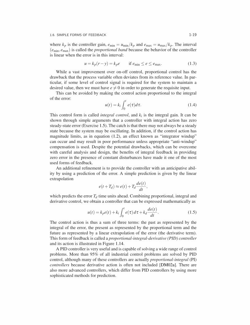
An additional refinement is to provide the controller with an anticipative abil-ity by using a prediction of the error. A simple prediction is given by the linearextrapolation

e(t +Td)≈ e(t)+Tdde(t)

dt,

which predicts the error Td time units ahead. Combining proportional, integral andderivative control, we obtain a controller that can be expressed mathematically as

u(t) = kpe(t)+ ki

∫ t

0e(τ)dτ + kd

de(t)

dt. (1.5)

The control action is thus a sum of three terms: the past as represented by theintegral of the error, the present as represented by the proportional term and thefuture as represented by a linear extrapolation of the error (the derivative term).This form of feedback is called a proportional-integral-derivative (PID) controllerand its action is illustrated in Figure 1.14.

A PID controller is very useful and is capable of solving a wide range of controlproblems. More than 95% of all industrial control problems are solved by PIDcontrol, although many of these controllers are actually proportional-integral (PI)controllers because derivative action is often not included [DM02a]. There arealso more advanced controllers, which differ from PID controllers by using moresophisticated methods for prediction.

1-20 CHAPTER 1. INTRODUCTION

Time

Error Present

FuturePast

t t +Td

Figure 1.14: Action of a PID controller. At time t, the proportional term depends on theinstantaneous value of the error. The integral portion of the feedback is based on the integralof the error up to time t (shaded portion). The derivative term provides an estimate of thegrowth or decay of the error over time by looking at the rate of change of the error. Td

represents the approximate amount of time in which the error is projected forward (see text).

1.7 Combining Feedback with Logic

The PID controller is a continuous time system. The on-off controller can beviewed both as a controller and a logic system. Continuous control is often com-bined with logic to cope with different operating conditions. Logic is typicallyrelated to changes in operating conditions, equipment protection, manual interac-tion and saturating actuators. One situation is when there is one variable that isof primary interest, but other variables may have to be controlled for equipmentprotection. For example, when controlling a compressor the outflow is the primaryvariable but it may be necessary to switch to a different mode to avoid compressorstall, which may damage the compressor. We illustrate some ways in which logicand feedback are combined by a few examples.

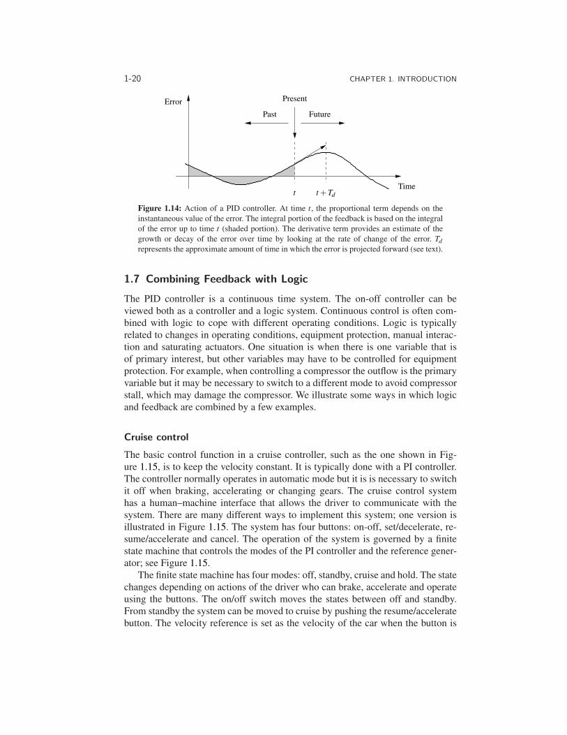
Cruise control

The basic control function in a cruise controller, such as the one shown in Fig-ure 1.15, is to keep the velocity constant. It is typically done with a PI controller.The controller normally operates in automatic mode but it is is necessary to switchit off when braking, accelerating or changing gears. The cruise control systemhas a human–machine interface that allows the driver to communicate with thesystem. There are many different ways to implement this system; one version isillustrated in Figure 1.15. The system has four buttons: on-off, set/decelerate, re-sume/accelerate and cancel. The operation of the system is governed by a finitestate machine that controls the modes of the PI controller and the reference gener-ator; see Figure 1.15.

The finite state machine has four modes: off, standby, cruise and hold. The statechanges depending on actions of the driver who can brake, accelerate and operateusing the buttons. The on/off switch moves the states between off and standby.From standby the system can be moved to cruise by pushing the resume/acceleratebutton. The velocity reference is set as the velocity of the car when the button is

1.7. COMBINING FEEDBACK WITH LOGIC 1-21

cancel

StandbyOff

Cruise

Hold

on

off

off

off

set

brake resume

Figure 1.15: Finite state machine for cruise control system. The figure on the left showssome typical buttons used to control the system. The controller can be in one of four modes,corresponding to the nodes in the diagram on the right. Transition between the modes iscontrolled by pressing one of the five buttons on the cruise control interface: on, off, set,resume or cancel.

released. In the cruise state the operator can change the velocity reference; it isincreased by the button resume/accelerate and decreased by the button set/coast.If the driver accelerates by pushing the gas pedal the speed increases but it willgo back to the set velocity when the gas pedal is released. If the driver brakes thecar brakes and the cruise controller goes into hold but it remembers the set pointof the controller; it can be brought to the cruise state by pushing the res/acceleratebutton. The system also moves from cruise mode to standby if the cancel button ispushed. The reference for the velocity controller is remembered. The system goesinto off mode by pushing off.

The PI controller is designed to have good regulation properties and to givegood transient performance when switching between resume and control modes.

Server Farms

Server farms consist of a large number of computers for providing Internet services(cloud computing). Large server farms may have thousands of processors. Powerconsumption for driving the servers and for cooling them is a prime concern. Thecost for energy can be more than 40% of the total cost for data centers, whichis of the order of a million dollars per month for a large installation [EKR03].The prime task of the server farm is to respond to a strongly varying computingdemand. There are constraints given by electricity consumption and the availablecooling capacity. The throughput of an individual server depends on the clock rate,which can be changed by the voltage applied to the system. Increasing the supplyvoltage increases the energy consumption and more cooling is required.

Control of server farms is often performed using a combination of feedbackand logic. Capacity can be increased rapidly if a server is switched on simply byincreasing the voltage to a server, but a server that is switched on consumes energyand requires cooling. Control of server farms is often performed by a combinationof feedback and logic. To save energy it is advantageous to switch off serversthat are not required, but it takes some time to switch on a new server. A controlsystem for a server farm requires individual control of the voltage and coolingof each server and a strategy for switching servers on and off. Temperature is

1-22 CHAPTER 1. INTRODUCTION

Oil

Air

PI

PI

MAX

MIN

Y

R

Y

R

r

(a) Block diagram

0 10 20 300

0.5

1

y

0 10 20 300

0.5

1

t

u

(b) Step response

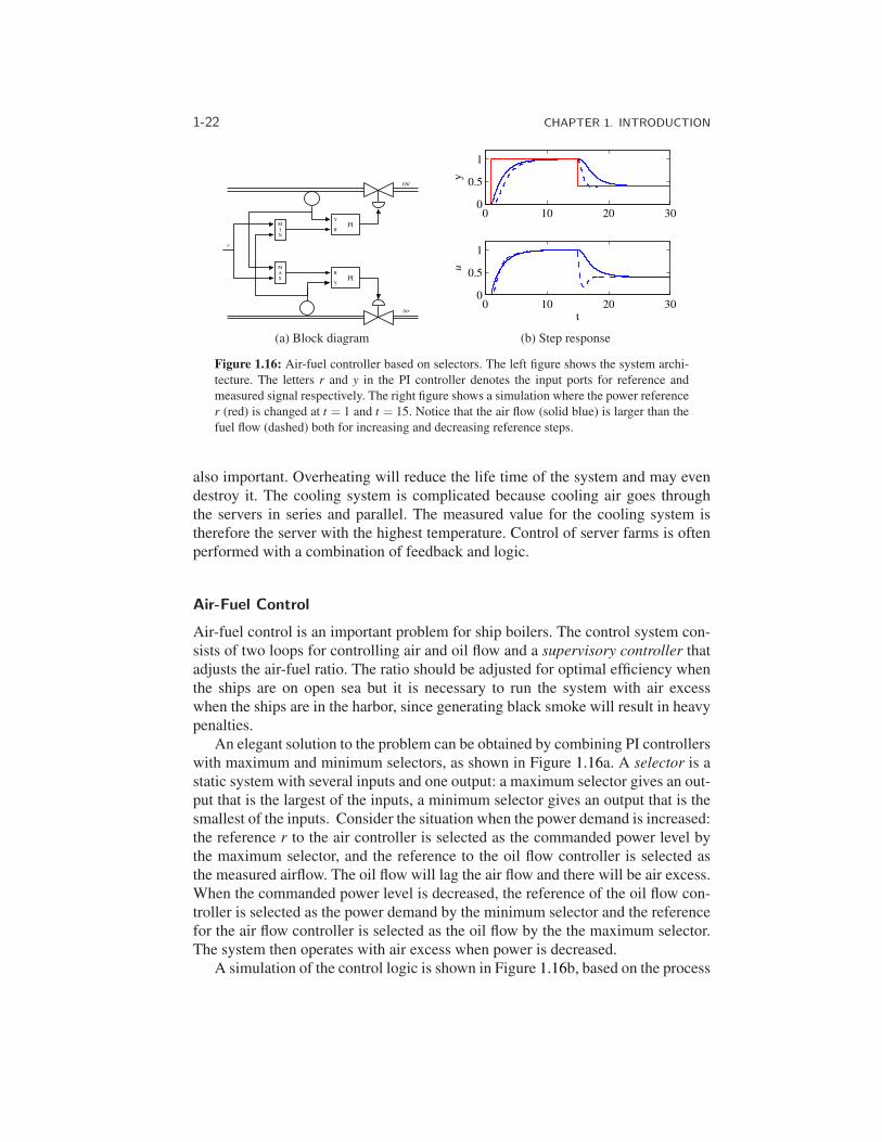
Figure 1.16: Air-fuel controller based on selectors. The left figure shows the system archi-tecture. The letters r and y in the PI controller denotes the input ports for reference andmeasured signal respectively. The right figure shows a simulation where the power referencer (red) is changed at t = 1 and t = 15. Notice that the air flow (solid blue) is larger than thefuel flow (dashed) both for increasing and decreasing reference steps.

also important. Overheating will reduce the life time of the system and may evendestroy it. The cooling system is complicated because cooling air goes throughthe servers in series and parallel. The measured value for the cooling system istherefore the server with the highest temperature. Control of server farms is oftenperformed with a combination of feedback and logic.

Air-Fuel Control

Air-fuel control is an important problem for ship boilers. The control system con-sists of two loops for controlling air and oil flow and a supervisory controller thatadjusts the air-fuel ratio. The ratio should be adjusted for optimal efficiency whenthe ships are on open sea but it is necessary to run the system with air excesswhen the ships are in the harbor, since generating black smoke will result in heavypenalties.

An elegant solution to the problem can be obtained by combining PI controllerswith maximum and minimum selectors, as shown in Figure 1.16a. A selector is astatic system with several inputs and one output: a maximum selector gives an out-put that is the largest of the inputs, a minimum selector gives an output that is thesmallest of the inputs. Consider the situation when the power demand is increased:the reference r to the air controller is selected as the commanded power level bythe maximum selector, and the reference to the oil flow controller is selected asthe measured airflow. The oil flow will lag the air flow and there will be air excess.When the commanded power level is decreased, the reference of the oil flow con-troller is selected as the power demand by the minimum selector and the referencefor the air flow controller is selected as the oil flow by the the maximum selector.The system then operates with air excess when power is decreased.

A simulation of the control logic is shown in Figure 1.16b, based on the process

1.8. CONTROL SYSTEM ARCHITECTURES 1-23

modeldxa

dt=−4xa +4ua,

dxo

dt=−xo +uo,

where xa and xo are the states representing air and oil dynamics. The air dynamicsare faster than the oil dynamics. The PI controllers are described by

ua =−kpaxa + kia

∫ t

(ra− ya)dt, ra = max(r,x0),

uo =−kpoxo + kio

∫ t

(ro− yo)dt, ro = min(r,xa).

The controller gains used in are kpa = 1, kia = 1, kpo = 2 and kio = 4.Selectors are commonly used to implement logic in engines and power systems.

They are also used for systems that require very high reliability: by introducingthree sensors and only accepting values where two sensors agree it is possible toguard for the failure of a single sensor.

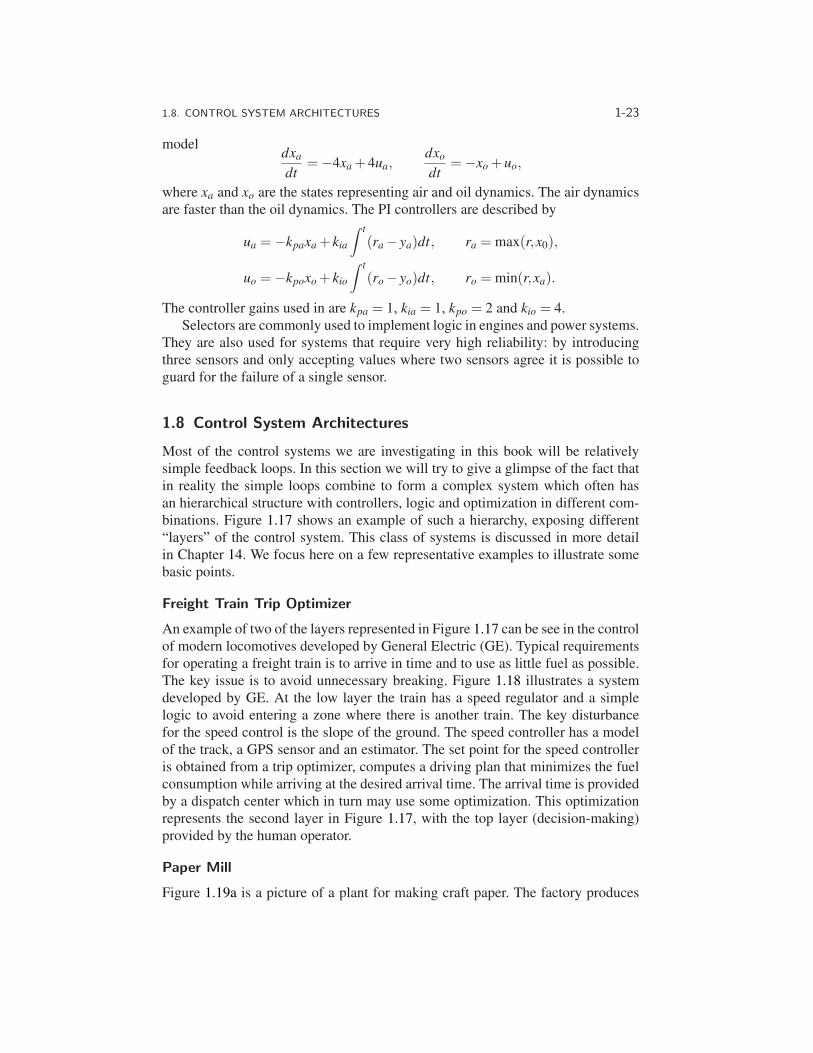
1.8 Control System Architectures

Most of the control systems we are investigating in this book will be relativelysimple feedback loops. In this section we will try to give a glimpse of the fact thatin reality the simple loops combine to form a complex system which often hasan hierarchical structure with controllers, logic and optimization in different com-binations. Figure 1.17 shows an example of such a hierarchy, exposing different“layers” of the control system. This class of systems is discussed in more detailin Chapter 14. We focus here on a few representative examples to illustrate somebasic points.

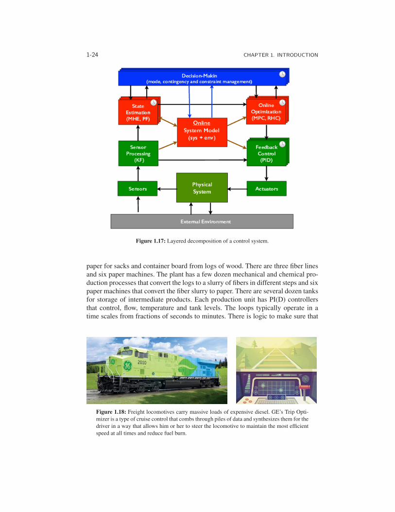
Freight Train Trip Optimizer

An example of two of the layers represented in Figure 1.17 can be see in the controlof modern locomotives developed by General Electric (GE). Typical requirementsfor operating a freight train is to arrive in time and to use as little fuel as possible.The key issue is to avoid unnecessary breaking. Figure 1.18 illustrates a systemdeveloped by GE. At the low layer the train has a speed regulator and a simplelogic to avoid entering a zone where there is another train. The key disturbancefor the speed control is the slope of the ground. The speed controller has a modelof the track, a GPS sensor and an estimator. The set point for the speed controlleris obtained from a trip optimizer, computes a driving plan that minimizes the fuelconsumption while arriving at the desired arrival time. The arrival time is providedby a dispatch center which in turn may use some optimization. This optimizationrepresents the second layer in Figure 1.17, with the top layer (decision-making)provided by the human operator.

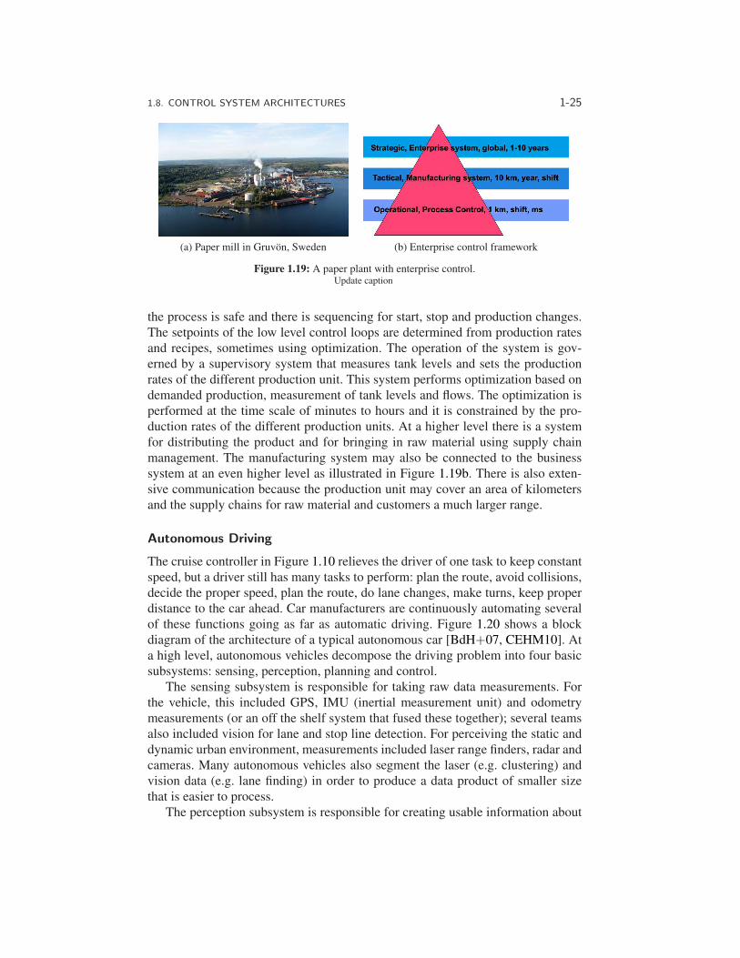
Paper Mill

Figure 1.19a is a picture of a plant for making craft paper. The factory produces

1-24 CHAPTER 1. INTRODUCTION

Figure 1.17: Layered decomposition of a control system.

paper for sacks and container board from logs of wood. There are three fiber linesand six paper machines. The plant has a few dozen mechanical and chemical pro-duction processes that convert the logs to a slurry of fibers in different steps and sixpaper machines that convert the fiber slurry to paper. There are several dozen tanksfor storage of intermediate products. Each production unit has PI(D) controllersthat control, flow, temperature and tank levels. The loops typically operate in atime scales from fractions of seconds to minutes. There is logic to make sure that

Figure 1.18: Freight locomotives carry massive loads of expensive diesel. GE’s Trip Opti-mizer is a type of cruise control that combs through piles of data and synthesizes them for thedriver in a way that allows him or her to steer the locomotive to maintain the most efficientspeed at all times and reduce fuel burn.

1.8. CONTROL SYSTEM ARCHITECTURES 1-25

(a) Paper mill in Gruvon, Sweden (b) Enterprise control framework

Figure 1.19: A paper plant with enterprise control.Update caption

the process is safe and there is sequencing for start, stop and production changes.The setpoints of the low level control loops are determined from production ratesand recipes, sometimes using optimization. The operation of the system is gov-erned by a supervisory system that measures tank levels and sets the productionrates of the different production unit. This system performs optimization based ondemanded production, measurement of tank levels and flows. The optimization isperformed at the time scale of minutes to hours and it is constrained by the pro-duction rates of the different production units. At a higher level there is a systemfor distributing the product and for bringing in raw material using supply chainmanagement. The manufacturing system may also be connected to the businesssystem at an even higher level as illustrated in Figure 1.19b. There is also exten-sive communication because the production unit may cover an area of kilometersand the supply chains for raw material and customers a much larger range.

Autonomous Driving

The cruise controller in Figure 1.10 relieves the driver of one task to keep constantspeed, but a driver still has many tasks to perform: plan the route, avoid collisions,decide the proper speed, plan the route, do lane changes, make turns, keep properdistance to the car ahead. Car manufacturers are continuously automating severalof these functions going as far as automatic driving. Figure 1.20 shows a blockdiagram of the architecture of a typical autonomous car [BdH+07, CEHM10]. Ata high level, autonomous vehicles decompose the driving problem into four basicsubsystems: sensing, perception, planning and control.

The sensing subsystem is responsible for taking raw data measurements. Forthe vehicle, this included GPS, IMU (inertial measurement unit) and odometrymeasurements (or an off the shelf system that fused these together); several teamsalso included vision for lane and stop line detection. For perceiving the static anddynamic urban environment, measurements included laser range finders, radar andcameras. Many autonomous vehicles also segment the laser (e.g. clustering) andvision data (e.g. lane finding) in order to produce a data product of smaller sizethat is easier to process.

The perception subsystem is responsible for creating usable information about

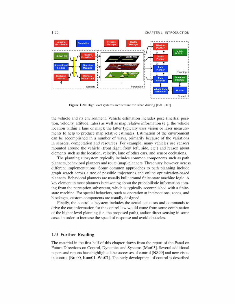
1-26 CHAPTER 1. INTRODUCTION

Figure 1.20: High level systems architecture for urban driving [BdH+07].

the vehicle and its environment. Vehicle estimation includes pose (inertial posi-tion, velocity, attitude, rates) as well as map relative information (e.g. the vehiclelocation within a lane or map); the latter typically uses vision or laser measure-ments to help to produce map relative estimates. Estimation of the environmentcan be accomplished in a number of ways, primarily because of the variationsin sensors, computation and resources. For example, many vehicles use sensorsmounted around the vehicle (front right, front left, side, etc.) and reason aboutelements such as the location, velocity, lane of other cars, and sensor occlusions.

The planning subsystem typically includes common components such as pathplanners, behavioral planners and route (map) planners. These vary, however, acrossdifferent implementations. Some common approaches to path planning includegraph search across a tree of possible trajectories and online optimization-basedplanners. Behavioral planners are usually built around finite-state machine logic. Akey element in most planners is reasoning about the probabilistic information com-ing from the perception subsystem, which is typically accomplished with a finite-state machine. For special behaviors, such as operation at intersections, zones, andblockages, custom components are usually designed.

Finally, the control subsystem includes the actual actuators and commands todrive the car; information for the control law would come from some combinationof the higher level planning (i.e. the proposed path), and/or direct sensing in somecases in order to increase the speed of response and avoid obstacles.

1.9 Further Reading

The material in the first half of this chapter draws from the report of the Panel onFuture Directions on Control, Dynamics and Systems [Mur03]. Several additionalpapers and reports have highlighted the successes of control [NS99] and new vistasin control [Bro00, Kum01, Wis07]. The early development of control is described

EXERCISES 1-27

by Mayr [May70] and in the books by Bennett [Ben79, Ben93], which cover theperiod 1800–1955. A fascinating examination of some of the early history of con-trol in the United States has been written by Mindell [Min02]. A popular bookthat describes many control concepts across a wide range of disciplines is Out ofControl by Kelly [Kel94].

There are many textbooks available that describe control systems in the con-text of specific disciplines. For engineers, the textbooks by Franklin, Powell andEmami-Naeini [FPEN05], Dorf and Bishop [DB04], Kuo and Golnaraghi [KG02]and Seborg, Edgar and Mellichamp [SEM04] are widely used. More mathemati-cally oriented treatments of control theory include Sontag [Son98] and Lewis [Lew03].The books by Hellerstein et al. [HDPT04] and Janert [Jan14] provide descriptionsof the use of feedback control in computing systems. A number of books look at therole of dynamics and feedback in biological systems, including Milhorn [Mil66](now out of print), J. D. Murray [Mur04] and Ellner and Guckenheimer [EG05].The book by Fradkov [Fra07] and the tutorial article by Bechhoefer [Bec05] covermany specific topics of interest to the physics community.

Systems that combine continuous feedback with logic and sequencing are calledhybrid systems [RST12]. The theory required to properly model and analyze suchsystems is outside the scope of this book. It is, however, very common that practi-cal control systems combine feedback control with logic sequencing and selectors;many examples are given in [AH05].

Exercises

1.1 (Eye motion) Perform the following experiment and explain your results: Hold-ing your head still, move one of your hands left and right in front of your face,following it with your eyes. Record how quickly you can move your hand beforeyou begin to lose track of it. Now hold your hand still and shake your head left toright, once again recording how quickly you can move before losing track of yourhand.

1.2 Identify five feedback systems that you encounter in your everyday environ-ment. For each system, identify the sensing mechanism, actuation mechanism andcontrol law. Describe the uncertainty with respect to which the feedback systemprovides robustness and/or the dynamics that are changed through the use of feed-back.

1.3 (Balance systems) Balance yourself on one foot with your eyes closed for 15 s.Using Figure 1.3 as a guide, describe the control system responsible for keepingyou from falling down. Note that the “controller” will differ from that in the dia-gram (unless you are an android reading this in the far future).

1.4 (Cruise control) Download the MATLAB code used to produce simulations forthe cruise control system in Figure 1.10 from the companion web site. Using trialand error, change the parameters of the control law so that the overshoot in speedis not more than 1 m/s for a vehicle with mass m = 1000 kg.

1-28 CHAPTER 1. INTRODUCTION

1.5 (Integral action) We say that a system with a constant input reaches steadystate if all system variables approach constant values as time increases. Show thata controller with integral action, such as those given in equations (1.4) and (1.5),gives zero error if the closed loop system reaches steady state. Notice that there isno saturation in the controller.

1.6 Search the web and pick an article in the popular press about a feedback andcontrol system. Describe the feedback system using the terminology given in thearticle. In particular, identify the control system and describe (a) the underlyingprocess or system being controlled, along with the (b) sensor, (c) actuator and (d)computational element. If the some of the information is not available in the article,indicate this and take a guess at what might have been used.