Embed Size (px)
Citation preview

i
STATE ESTIMATION BASED FAULT LOCATION USING PMU
MEASUREMENTS
A THESIS SUBMITTED TO
THE GRADUATE SCHOOL OF NATURAL AND APPLIED SCIENCES
OF
MIDDLE EAST TECHNICAL UNIVERSITY
BY
AHMET ÖNER
IN PARTIAL FULFILLMENT OF THE REQUIREMENTS
FOR
THE DEGREE OF MASTER OF SCIENCE
IN
ELECTRICAL AND ELECTRONICS ENGINEERING
JULY 2016

ii

iii
Approval of the thesis:
STATE ESTIMATION BASED FAULT LOCATION USING PMU
MEASUREMENTS
submitted by AHMET ÖNER in partial fulfillment of the requirements for the
degree of Master of Science in Electrical and Electronics Engineering
Department, Middle East Technical University by,
Prof. Dr. Gülbin Dural Ünver _____________
Dean, Graduate School of Natural and Applied Sciences
Prof. Dr. Gönül Turhan Sayan _____________
Head of Department, Electrical and Electronics Engineering
Assist. Prof. Dr. Murat Göl _____________
Supervisor, Electrical and Electronics Eng. Dept., METU
Examining Committee Members:
Prof. Dr. Nezih Güven _____________
Electrical and Electronics Engineering Dept., METU
Assist. Prof. Dr. Murat Göl _____________
Electrical and Electronics Engineering Dept., METU
Assoc. Prof. Dr. Özgül Salor Durna _____________
Electrical and Electronics Engineering Dept., Gazi University
Assoc. Prof. Dr. Umut Orguner _____________
Electrical and Electronics Engineering Dept., METU
Assist. Prof. Dr. Ozan Keysan _____________
Electrical and Electronics Engineering Dept., METU
Date: 12.07.2016

iv
I hereby declare that all information in this document has been obtained and
presented in accordance with academic rules and ethical conduct. I also declare
that, as required by these rules and conduct, I have fully cited and referenced
all material and results that are not original to this work.
Name, Last Name : AHMET ÖNER
Signature :

v
ABSTRACT
STATE ESTIMATION BASED FAULT LOCATION USING PMU
MEASUREMENTS
Öner, Ahmet
M.Sc., Department of Electrical & Electronics Engineering
Supervisor : Assist. Prof. Dr. Murat Göl
July 2016, 60 Pages
Accurate location of a permanent fault on a transmission line is extremely important
to restore the service in the shortest time possible, which directly affects the
operational cost and system reliability. There are measurement based fault location
methods in the literature, which require a high number of installed devices at
substations. In this thesis study, an accurate and computationally fast strategy for
fault location based on well-known Weighted Least Squares state estimator is
presented.
The proposed method employs Phasor Measurement Unit (PMU) measurements
recorded during the fault, due to the fast refresh rate of PMUs. PMUs provide
synchronized voltage and current measurements. The synchronization of the PMU
measurements is achieved using Global Positioning System (GPS). Those
measurements are used to identify the faulted line via the estimated current flows in
the system and then locate the fault on the flagged line disregarding the value of the
fault impedance.
The proposed method makes use of multiple PMU measurements received in
consecutive time instants and hence reduces the required number of measurements
for the solution of the fault location problem. Moreover, use of those multiple
measurements improves the robustness of the proposed method against the bad data
and incorrect parameters.
The fault location problem is also solved with a modified formulation in order to
show the robustness of the proposed method against the incorrect line parameters.
The modified formulation includes estimation of the line parameters with multiple
PMU measurements.

vi
The proposed method has an iterative solution, because of the non-linearity between
the measurements and the states to be determined. This thesis also shows the
importance of the initial values and indicates comments on selection of those values.
The proposed method is validated using synthetic data in different computational
environments.
Keywords: Fault Location, Least Squares Estimation, Phasor Measurement Units
(PMU), State Estimation

vii
ÖZ
FAZÖR ÖLÇÜM BİRİMİ ÖLÇÜMLERİ İLE DURUM KESTİRİMİ TEMELLİ
HATA LOKALİZASYONU
Öner, Ahmet
Yüksek Lisans, Elektrik & Elektronik Mühendisliği Bölümü
Tez Yöneticisi : Yard. Doç. Dr. Murat Göl
Temmuz 2016, 60 Sayfa
Bir iletim hattı üzerindeki daimi hatanın en kısa sürede onarılabilmesi için hatanın
doğru bir şekilde lokalize edilmesi önem arz etmektedir. Hatanın en kısa sürede
onarılması işletme maliyetini ve sistem güvenilirliğini doğrudan etkilemektedir.
Literatürde, trafo merkezlerine yüksek miktarda ölçüm cihazı kurulumu gerektiren
ölçüm temelli hata lokalizasyonu methodları bulunmaktadır. Bu tez çalışmasında,
Ağırlıklandırılmış En Küçük Kareler durum kestirimi methoduna dayalı hata
lokalizasyonunun hassas ve hızlı hesaplanabilir bir yöntemi sunulmaktadır.
Önerilen method, Fazör Ölçüm Birimlerinin yüksek yenilenme hızı sayesinde, hata
sırasında kaydettiği ölçümleri kullanmaktadır. Fazör Ölçüm Birimleri, senkronize
voltaj ve akım ölçümleri sağlamaktadır. Fazör Ölçüm Birimi ölçümlerinin
senkronizasyonu Küresel Konumlama Sistemi kullanılarak gerçekleştirilmektedir. Bu
ölçümler, sistem üzerinde kestirimi yapılan akımlar üzerinden hatalı hattın
belirlenmesinde kullanılmaktadır. Daha sonra, hatalı olarak işaretlenen hattın hata
konumu, hata empedansı ihmal edilerek bulunmaktadır.
Önerilen method, Fazör Ölçüm Birimlerinin art arda ölçüm alabilmesinden
faydalanmaktadır. Dolayısı ile hata lokalizasyonu probleminin çözümü için ihtiyaç
duyulan ölçüm sayısını azaltmaktadır. Buna ek olarak, birden çok ölçümün
kullanılması hatalı veriye ve yanlış parametrelere karşı gürbüzlük sağlamaktadır.
Önerilen methodun hatalı veri altında gürbüzlüğünü göstermek amacıyla hata
lokalizasyonu problemi modifiye edilmiş formülasyon ile de çözülmüştür.
Formülasyondaki değişiklik Fazör Ölçüm Birimlerinin art arda ölçüm alabilmesinden
faydalanarak hat parametrelerinin kestirimini içermektedir.

viii
Önerilen method, ölçümler ve hata konumları arasındaki doğrusal olmayan ilişki
sebebiyle yinelemeli çözüme sahiptir. Bu tez, aynı zamanda başlangıç değerlerinin
önemini göstermekte olup bu değerlerin seçim işlemini yorumlamaktadır.
Önerilen method, farklı ortamlardaki yapay veriler kullanılarak doğrulanmıştır.
Anahtar Kelimeler: Hata Lokalizasyonu, En Küçük Kareler Kestirimi, Fazör Ölçüm
Birimleri, Durum Kestirimi

ix
To My Family

x
ACKNOWLEDGMENTS
First of all, I would like to thank and express my deepest gratitude to my supervisor
and mentor Murat Göl, for his support, guidance and encouragement. His guidance
will shape my future.
I thank my parents for their endless trust and support throughout my life. I also
would like to thank my brother, Alper, for his help and patience during my studies.
I am also grateful to ASELSAN Inc. for her opportunities and supports during the
completion of this thesis.
xi
TABLE OF CONTENTS
ABSTRACT ................................................................................................................. v
ÖZ .............................................................................................................................. vii
ACKNOWLEDGMENTS ........................................................................................... x
TABLE OF CONTENTS ............................................................................................ xi
LIST OF TABLES .................................................................................................... xiii
LIST OF FIGURES .................................................................................................. xiv
LIST OF ABBREVIATIONS ................................................................................... xvi
CHAPTERS
1. INTRODUCTION ................................................................................................ 1
2. BACKGROUND .................................................................................................. 7
2.1 Problem Statement ........................................................................................ 7
2.2 Weighted Least Squares (WLS) .................................................................... 8
2.3 Iterative Solution of WLS (Gauss-Newton Method)..................................... 9
2.4 Normalized Residual Test ........................................................................... 11
3. THE PROPOSED METHOD ............................................................................. 15
3.1 State Estimation Based Identification of Faulted Lines .............................. 15
3.2 Fault Location on a Transmission Line Based on State Estimation ............ 20
4. SIMULATION RESULTS ................................................................................. 27

xii
4.1 Verification of the Proposed Faulted Line Identification Method .............. 31
4.2 Verification of the Proposed Fault Location Method .................................. 38
4.3 Effect of Incorrect Line Parameters on the Proposed Method .................... 46
4.4 Effect of Multiple Faults on the Proposed Method ..................................... 51
4.5 Discussion .................................................................................................... 52
5. CONCLUSION ................................................................................................... 55
REFERENCES ........................................................................................................... 57
xiii
LIST OF TABLES
TABLES
Table 4-1 Bus Data of IEEE 14 Bus Test Case System ............................................. 29
Table 4-2 Branch Data of IEEE 14 Bus Test Case System ....................................... 30
Table 4-3 pMAE for Different Fault Locations at Different Lines ............................ 32
Table 4-4 DigSilent Short Circuit Simulation Results for Different α Values .......... 35
Table 4-5 pMAE for a Given Fault Locations using DigSilent Data ......................... 35
Table 4-6 DigSilent Short Circuit Simulation Results for Different α Values .......... 36
Table 4-7 pMAE for a Given Fault Locations using DigSilent Data ......................... 37
Table 4-8 pMAE for Different Fault Location at a Given Line ................................. 38
Table 4-9 pMAE for Different Fault Location at a Given Line with incorrect
impedance .................................................................................................................. 50
Table 4-10 pMAE for a Given Fault Locations ......................................................... 52
xiv
LIST OF FIGURES
FIGURES
Figure 2-1 Summary of WLS State Estimation Algorithm ........................................ 10
Figure 3-1 Summary of State Estimation Based Identification of Faulted Lines ...... 19
Figure 3-2 Calculation of fault current using state estimates ..................................... 20
Figure 3-3 Sample faulted line ................................................................................... 21
Figure 3-4 Sample fault current time variation .......................................................... 22
Figure 4-1 IEEE 14 Bus Test Case System ................................................................ 28
Figure 4-2 Error Between Estimated Location and Real Location for Different Lines
(α0: 0.005, α: 0.5) ....................................................................................................... 32
Figure 4-3 Error Between Estimated Location and Real Location for Different Lines
(α0: 0.05, α: 0.95) ....................................................................................................... 33
Figure 4-4 A Sample Screenshot of DigSilent while Short Circuit Analysis ............ 34
Figure 4-5 Performance of the Algorithm with DigSilent Data for Fault Between
Bus-1 and Bus-2 ......................................................................................................... 36
Figure 4-6 Performance of the Algorithm with DigSilent Data for Fault Between
Bus-7 and Bus-8 ......................................................................................................... 37
Figure 4-7 Error Between Estimated Location and Real Location for α0 = 0.005 ..... 39
Figure 4-8 Error Between Estimated Location and Real Location for α0 = 0.01 ....... 40
Figure 4-9 Error Between Estimated Location and Real Location for α0 = 0.02 ....... 41

xv
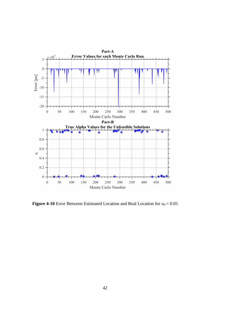
Figure 4-10 Error Between Estimated Location and Real Location for α0 = 0.05 ..... 42
Figure 4-11 Error Between Estimated Location and Real Location for α0 = 0.99 ..... 43
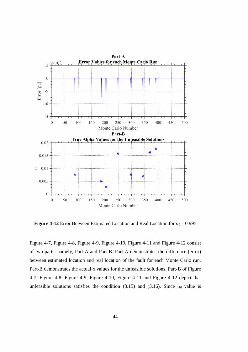
Figure 4-12 Error Between Estimated Location and Real Location for α0 = 0.995 ... 44
Figure 4-13 Error Between Estimated Location and Real Location for varied α0 ..... 45
Figure 4-14: Error Between Estimated Location and Real Location with Incorrect
Impedance .................................................................................................................. 51

xvi
LIST OF ABBREVIATIONS
ANSI : American National Standards Institute
BLUE : Best Linear Unbiased Estimator
EMS : Energy Management System
GPS : Global Positioning System
IEEE : Institute of Electrical and Electronics Engineers
LAV : Least Absolute Value
MAE : Mean Absolute Error
pMAE : Percentage Mean Absolute Error
PMU : Phasor Measurement Unit
SCADA : Supervisory control and data acquisition
SE : State Estimation
WLS : Weighted Least Squares
1
CHAPTER 1
1. INTRODUCTION
In recent years, power systems in the world have rapidly grown due to the raise in the
electricity demand, which resulted in complicated system structures with a very high
number of transmission lines. Those lines are exposed to faults in different ways
such as lightning strokes, storms and short circuits due to contacts of trees, which
may cause permanent faults on the transmission lines. To be able to clear the
permanent faults in the shortest time, and to improve the power quality, system
security and the reliability of the grid, fault location is required. In the literature
many fault location methods are presented [1] – [24].
The fault location methods can be divided into two categories. Among the methods
presented in the literature, a good number of impedance-based fault location
algorithms, which are performed at the power frequency, have been developed [1] –
[16]. Those algorithms use bus voltage and line current data of either a single bus
(one-ended) [2] – [5] or both buses (two-ended) [6] – [10] that are connected to the
faulted line. Multi-bus algorithms, which use measurements taken from the ends of
the multi-terminal transmission lines, are also available in the literature [11] – [16].
The second group of the fault location methods is based on high-frequency
components of the fault-transient signals, which may be called traveling-wave based
fault-location methods [17] – [24]. Those methods use the correlation between
traveling waves, which propagate along the transmission lines. Although, those

2
methods are more accurate compared to impedance-based methods, they require
special equipment designed to collect raw data with acceptable precision, which
increases the cost of fault location significantly.
This thesis proposes use of two-terminal impedance-based fault location using
Phasor Measurement Unit (PMU) data, which are populating in power systems since
2003. PMUs measure synchronized voltage and current phasor measurements with
respect to the Global Positioning System (GPS), which provides access to an
accurate global clock. They have a great advantage in managing the power system
thanks to their fast refresh rates. Typically, PMUs refreshing rate is 30 scans per
second [25] – [26].
The main motivation of the thesis is to identify faulted lines in a given system and
locate the faults on the identified lines to enable service providers restore the service
in the shortest time possible, which will increase the power quality and the reliability
of the grid. In order to reduce the effects of the measurement errors, and incorrect
system parameter information, which is quite possible due to varying weather
conditions, this work employs state estimation methods to identify the faulted lines
and locate the faults along the identified transmission lines.
For power quality, system security and sustainability, and reliability of the service,
Energy Management System (EMS) is used to monitor, control and optimize the
performance of the generation and transmission systems. Operators of EMS need
reliable information for proper operation. Therefore, state estimation is one of the
most important tools of the EMS. State estimators;
Estimate bus voltages, branch flows, etc. (state variables),
Provide measurement error processing results,
Give an estimate for all metered and unmetered quantities,

3
Filter out small errors due to model approximations and measurement
inaccuracies,
Detect and identify discordant measurements, called bad data.
This thesis proposes a state estimation based fault location method, which employs
the well-known two-ended algorithm [6] – [10]. The method assumes that the
considered system is PMU observable, such that the state estimation can be
performed using only PMU measurements. Considering the increasing number of
PMUs, it can be expected that this assumption will be realized in near future for
many grids around the world. Use of PMUs enables use of measurements received at
different time instants for fault location, which contributes the robustness to the state
estimator. Moreover, thanks to the time synchronization in PMU observable systems,
the fault location can be performed more accurately compared to the systems
measured by conventional SCADA measurements.
The proposed method firstly performs power system state estimation [27] to
determine the voltages of each bus, which may be called as EMS state estimator.
Assuming the considered system’s measurement design is redundant enough, such
that bad data can be identified, the fundamental component of the faulted current
flowing through the line from both sending and receiving ends can be calculated.
Note that this part is especially necessary if sending end and/or receiving end of the
faulted line is not measured by a PMU.
Once the faulted line is identified, Weighted Least Squares (WLS) estimator is
employed to locate the fault on the identified transmission line. WLS uses estimates
of the line currents and bus voltages as well as the measurements obtained from
PMUs corresponding to different time instants for measurement redundancy.
This thesis assumes that the conventional circuit breakers interrupt the fault current
at least in 4 cycles [28]. Therefore, 2 measurement scans from the PMUs and hence 2

4
estimation sets are available, which provide the observation redundancy to perform a
proper estimation.
State estimation was used for fault location previously [29]. The method in [29]
modifies the state vector, by adding new system states for the location of the fault
each time a fault is detected. If there is more than one fault in the system on different
lines, [29] may not be able to find the fault locations because of the decreased
redundancy, which may lead to an unobservable system. However, the proposed
algorithm can determine the fault location, independent of the number of faults, since
a separate state vector is formed for each fault.
The observation vector built by the proposed method includes current and voltage
phasor measurements collected in consecutive time instants, which provides the
observation redundancy to perform a proper estimation of the fault location.
Moreover, the estimation results obtained from the EMS state estimator may
contribute the measurement redundancy. Therefore, the proposed method never
experiences a redundancy problem. Moreover, thanks to the small size of the fault
location problem, the computational burden of the proposed method will be very
small. The fault locations are determined using WLS estimator, which is the Best
Linear Unbiased Estimator (BLUE) [30], such that the estimates will be the most
accurate if there is only Gaussian error associated with the measurements.
The main objectives of the thesis can be listed as follows:
Developing a state estimation based method to identify the faulted lines in a
given system
Locating the fault on the identified line, using state estimation.
The thesis consists of five chapters. Chapter 1 presents the thesis motivation and the
literature survey on fault location methods. Chapter 2 reviews the WLS state
estimation method and summarizes the iterative solution of WLS state estimation
method based on Gauss-Newton method. Chapter 3 introduces the proposed method

5
and explains how to identify faulted lines using estimated fault currents, and how to
build the fault location problem based on SE. Chapter 4 evaluates the performance of
proposed fault location based on SE technique which builds a separate state vector to
estimate the location of each fault. Finally, Chapter 5 consists of a summary of the
work and main conclusions drawn.


7
CHAPTER 2
2. BACKGROUND
After presenting the general introduction and fault location algorithm methods in
Chapter 1, this chapter will introduce the technical background, which will conduce
the reader understand the presented study. Firstly, problem statement will be
explained. Then, mathematical explanation of Weighted Least Squares (WLS)
method will be provided. Finally, Iterative Solution of WLS (Gauss-Newton
Method) approach will be introduced.
2.1 Problem Statement
This thesis investigates the problem of locating a fault in a power system using PMU
measurements. The methods proposed in the literature [1] – [16] are directly based
on the data obtained from the measurement devices. This work proposes use of state
estimation instead of measurements, in order to minimize the effects of measurement
and system model inaccuracies, and to decrease the number of devices that should be
installed in the system. Therefore, this work proposes performing power system state
estimation to determine the line flows that will point the faulted line. Then, the
estimated voltages and currents as well as the corresponding measurements are used
to locate the fault on the flagged transmission line. The Weighted Least Squares
(WLS) estimator is employed in this study because of its speed and ease of
8
implementation. Moreover, it is known that WLS is the best linear unbiased
estimator (BEST) under Gaussian noise [30]. The Weighted Least Squares and
Iterative Solution of WLS (Gauss-Newton Method) are reviewed in this chapter.
2.2 Weighted Least Squares (WLS)
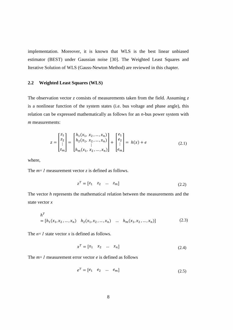
The observation vector z consists of measurements taken from the field. Assuming z
is a nonlinear function of the system states (i.e. bus voltage and phase angle), this
relation can be expressed mathematically as follows for an n-bus power system with
m measurements:
[
] [
] [
] (2.1)
where,
The m×1 measurement vector z is defined as follows.
[ ] (2.2)
The vector h represents the mathematical relation between the measurements and the
state vector x
[ ] (2.3)
The n×1 state vector x is defined as follows.
[ ] (2.4)
The m×1 measurement error vector e is defined as follows
[ ] (2.5)

9
It is assumed that:
- E[e] = 0
- Measurement errors are independent, i.e., E[eiej] = 0 where i≠j such that the
covariance matrix is diagonal:
[ ]
(2.6)
Based on those definitions, the WLS objective function is given as below.
∑
[ ]
[ ] (2.7)
The minimization condition of objective function is expressed below:
[ ] (2.8)
where H(x) = ∂h(x)/∂x.
2.3 Iterative Solution of WLS (Gauss-Newton Method)
In (2.8), expanding g(x) into its Taylor series around the state vector xk
gives the
following expression.
( ) ( )( ) (2.9)
Neglecting the higher order terms (H.O.T.) leads to an iterative solution:
( )
( ) (2.10)
where,
k is the iteration index,
xk is the solution vector at iteration k

10
G(xk) is the gain matrix, which is sparse, positive definite and symmetric if the
system is observable.
( ) ( )
( ) (2.11)
( ) ( ) (2.12)
The equation for the state estimation calculation is given by the expression
(2.13)
where Δxk+1
= xk+1
- xk
Figure 2-1 Summary of WLS State Estimation Algorithm
1) Set k = 0
2) Initialize the state vector xk , typical a flat start
3) Calculate the measurement function h(xk)
4) Build the measurement Jacobian H(xk)
5) Calculate the gain matrix of G(xk) = HT(xk)R-1H(xk)
6) Calculate HT(xk)R-1(z-h(xk))
7) Solve the equation for Δxk
8) Check for convergence using max |Δxk| ≤ ε
9) If not converged, update xk+1 = xk + Δxk and go to step 3. Otherwise stop

11
The WLS state estimation algorithm steps are summarized in Figure 2-1.
2.4 Normalized Residual Test
After the estimation process, state estimator may be deceived because of bad data. To
detect the bad data, normalized residual test is performed.
In (2.14), linearized measurement model is given,
(2.14)
where, is measurement vector,
is the true state vector,
H is Jacobian Matrix,
e is Gaussian error,
such that E[e]=0 and cov(e)=R.
The WLS estimate can be found based on the linearized measurement model as
follows.
⏟
(2.15)
(2.16)
The estimated value of is given in (2.17),
(2.17)
where K = HG-1
HTR
-1
The properties of K matrix are given below:
- K.K.K.K…K = K
- K.H = H

12
- (I-K).H =0
The measurement residuals can be computed as given in (2.18),
(I-K).H =0)
(2.18)
where S is the residual sensitivity matrix.
The properties of S matrix are given below:
- S.S.S.S…S = S
- S.R.ST = S.R
(2.19)
[ ]
[ ]
(2.20)
Therefore, r ~ N(0,Ω) where Ω is residual covariance matrix.
| |
√
| |
√
(2.21)
The normalized residual vector rN will have a Standart Normal Distribution,
riN ~ N(0,1).

13
Therefore, a comparison between rN
and a statistical threshold can find the bad data if
it exists. This threshold can be chosen based on the desired level of detection
sensitivity.

14
15
CHAPTER 3
3. THE PROPOSED METHOD
Chapter 2 described the problem, locating a fault in a power system using PMU
measurements, and also described the solution technique for the problem. As
mentioned in Chapter 1, in order to solve the problem and determine the fault
location, Weighted Least Squares (WLS) estimator is employed. In this chapter, the
stages of the proposed method will be explained. Firstly, the method to determine the
fault currents and hence identify the faulted line will be explained. Then, the fault
location based on state estimation on the identified transmission line will be
explained in detail.
3.1 State Estimation Based Identification of Faulted Lines
Identification of the faulted line is conducted based on the circuit breaker status in a
well-monitored power system. This work proposes use of fault current estimates to
determine the faulted line in the interconnected system using well-known WLS
estimator. Note that for a proper operation of an Energy Management System a
properly running state estimator is required. The proper state estimator consists of
observability analysis, state estimation, which is assumed to be WLS in this work,
and bad data analysis [27]. The proposed method makes use of state estimation and
bad data analysis tools of EMS.

16
To be able to run the state estimator and hence compute the line currents,
transmission system model, i.e. system connectivity and parameters (branch
resistance, branch reactance, shunt conductance, shunt susceptance) are necessary.
Moreover, the system should be observable, such that there should be a unique
solution of the state estimation problem. This thesis assumes that the considered
systems are PMU observable, such that the state estimation can be performed using
only PMU measurements. Note that considering the rapid increase of the
synchropahor measurements in the transmission grids, this assumption will be
applicable in the near future for many transmission grids around the world. Minimum
number of PMUs and installation locations can be found using [31].
PMU measurements are linearly related to the system states, which are bus voltage
phasors, on the contrary of the conventional power flow measurements. Therefore
the relation between the PMU measurements and the system states can be defined as
below:
(3.1)
where
[
] (3.2)
[
]
(3.3)

17
In (3.3),
- HPMU
is constant Jacobian matrix (with dimension 4m x 2n) for PMU only
systems where m is the number of measurement (for observable system) and
n is the number of buses of the power system.
- V is the solution vector where Vi and Vj are the solution voltages of 2 buses.
Note that, in (3.3), HPMU
is given for 2-Bus system.
Instead of computing each entry of (3.3), the relation between the bus voltages and
line current can be used to build HPMU
, which is defined as follows.
(
) (
)
(3.4)
(
) (
)
(3.5)
In (3.4) and (3.5),
- gij is the shunt conductance between Bus-i and Bus-j,
- bij is the shunt susceptance between Bus-i and Bus-j,
- bii is the half of the total line charging for Bus-i,
- Vii is the imaginary part of the system state voltage of Bus-i,
- Vir is the real part of the system state voltage of Bus-i,
- Vji is the imaginary part of the system state voltage of Bus-j,
- Vjr is the real part of the system state voltage of Bus-j,
- e is the measurement error,
- Iijm,r
is the real part of the measured current between Bus-i and Bus-j,
- Iijm,i
is the imaginary part of the measured current between Bus-i and Bus-j.
18
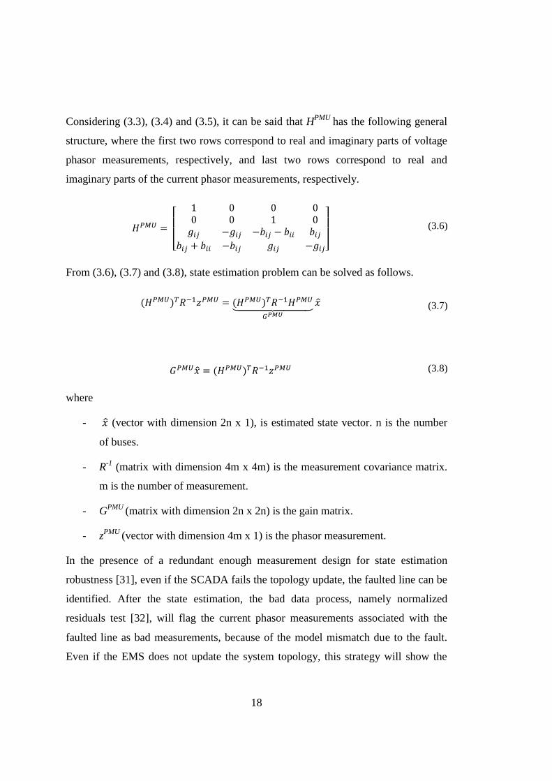
Considering (3.3), (3.4) and (3.5), it can be said that HPMU
has the following general
structure, where the first two rows correspond to real and imaginary parts of voltage
phasor measurements, respectively, and last two rows correspond to real and
imaginary parts of the current phasor measurements, respectively.
[
] (3.6)
From (3.6), (3.7) and (3.8), state estimation problem can be solved as follows.
⏟
(3.7)
(3.8)
where
- (vector with dimension 2n x 1), is estimated state vector. n is the number
of buses.
- R-1
(matrix with dimension 4m x 4m) is the measurement covariance matrix.
m is the number of measurement.
- GPMU
(matrix with dimension 2n x 2n) is the gain matrix.
- zPMU
(vector with dimension 4m x 1) is the phasor measurement.
In the presence of a redundant enough measurement design for state estimation
robustness [31], even if the SCADA fails the topology update, the faulted line can be
identified. After the state estimation, the bad data process, namely normalized
residuals test [32], will flag the current phasor measurements associated with the
faulted line as bad measurements, because of the model mismatch due to the fault.
Even if the EMS does not update the system topology, this strategy will show the
19
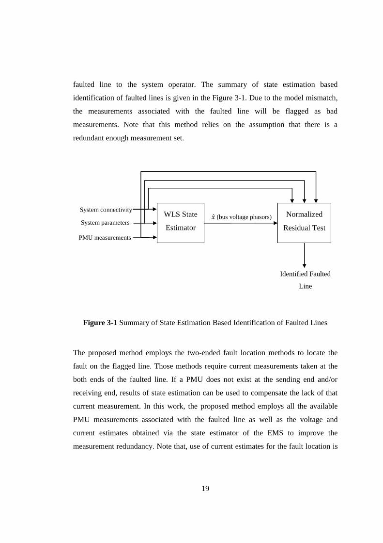
faulted line to the system operator. The summary of state estimation based
identification of faulted lines is given in the Figure 3-1. Due to the model mismatch,
the measurements associated with the faulted line will be flagged as bad
measurements. Note that this method relies on the assumption that there is a
redundant enough measurement set.
Figure 3-1 Summary of State Estimation Based Identification of Faulted Lines
The proposed method employs the two-ended fault location methods to locate the
fault on the flagged line. Those methods require current measurements taken at the
both ends of the faulted line. If a PMU does not exist at the sending end and/or
receiving end, results of state estimation can be used to compensate the lack of that
current measurement. In this work, the proposed method employs all the available
PMU measurements associated with the faulted line as well as the voltage and
current estimates obtained via the state estimator of the EMS to improve the
measurement redundancy. Note that, use of current estimates for the fault location is
Normalized
Residual Test
WLS State
Estimator System parameters
(bus voltage phasors)
Identified Faulted
Line
System connectivity
PMU measurements

20
possible if there is no power injection at the bus without PMU or the amount of
injected power is known.
Once the injection power is known, the fault current, If in Figure 3-2 can be
calculated as follows, using the famous Kirchhoff’s Current Law.
∑
(3.9)
In (3.9), N represents the set of lines connected to Bus-1. Note that, once the fault
occurs the system model corresponding to the faulted line will not be correct any
more. Therefore, the fault current cannot be calculated using the voltage estimates of
the sending and receiving end buses, but rather (3.9) should be employed.
Figure 3-2 Calculation of fault current using state estimates
3.2 Fault Location on a Transmission Line Based on State Estimation
The synchronized two-ended method solves the following two equations
simultaneously in order to locate the fault shown in Figure 3-3. In (3.10) and (3.11),
the transmission line is modelled as nominal Π. In nominal Π model, the total
lumped shunt admittance is divided into two equal halves, and each half with value
bii and bjj is placed at both the sending and the receiving end. In (3.10), Ifi is the

21
current flowing through sending end of the circuit. In other words, the total current of
Ifi is the sum of currents flowing through the admittances and currents flowing
through the impedance between the fault and sending end bus (Zα). In (3.11), Ifj is the
current flowing through receiving end of the circuit. The total current of Ifj is the sum
of the current flowing to the ground through the shunt admittance and the current
flowing through the impedance between the fault and receiving end bus (Z(1-α)).
(3.10)
(3.11)
where Vi, Vj and Vf are the voltage phasors at Bus-i, Bus-j and the fault location,
respectively. Fault current flowing through Bus-i is represented by Ifi, while fault
current flowing through Bus-j is represented by Ifj. Z represents the series impedance
of the line between buses i and j, and bii and bjj represent the line charging
susceptances at Bus-i and Bus-j, respectively. Finally, α shows the ratio of the
distance of the fault to Bus-i to the total length of the faulted line.
Figure 3-3 Sample faulted line
Conventional two-ended synchronized fault location solves (3.10) and (3.11) to find
α and Vf by disregarding the value of the fault impedance. It is known that PMU data
carry measurement error, which is assumed Gaussian. Moreover, due to the transient

22
during the clearance of the fault, calculated phasors may be erroneous. This work
proposes use of WLS estimator to calculate the fault location (α) in order to
minimize the effects of measurement errors.
Successful error removal requires measurement redundancy [31]. Therefore,
proposed method uses all measurements and state estimates, if required, recorded
from the beginning of the fault until the clearance of the fault. Considering the
opening time of a circuit breaker, the proposed method can use at least two PMU
scans for fault location as shown in Figure 3-4. Note that, Figure 3-4 is generated for
visualization purposes and it is not a result of simulation tool. If PMUs are re-
programmed to scan 60 times a second during a fault, instead of conventional
refreshing rate of 30 scans per second, the number of observations will be increased
to four and hence a more reliable estimation will be possible.
Figure 3-4 Sample fault current time variation
In Figure 3-4, “A” indicates the beginning time of the fault, and “B” shows the
duration that PMU measurements can be used, assuming that PMU refresh rate is 30
scans per second. During “B” two sets of voltage and current phasor measurements

23
will be received. The data recorded during “C” cannot be used, since some of it
includes data taken after the opening of the circuit breaker, which corresponds to the
point “D”. This work employs the measurements during “B” for fault location.
WLS estimator is employed to solve the non-linear estimation problem, where (3.10)
and (3.11) are the relations between the state vector and observation vector. The state
vector, x, is defined as follows.
[
] (3.12)
In (3.12);
1 , and 1
2 ,
mr
fV
, is the real part of the voltage phasor at the fault location at time instant-m,
mi
fV
, is the imaginary part of the voltage phasor at the fault location at time instant-m.
For two measurement scans from the PMUs, the state vector is as follows.
[
] (3.13)
In the proposed problem formulation observation vector consists of fault current
measurements and estimates, if necessary, taken at consecutive time instants.
[
] (3.14)
where
- Isr,1
is the real part of the measured current of sending end of the faulted line
at first time instant,
- Irr,1
is the real part of the measured current of receiving end of the faulted line
at first time instant,

24
- Isr,2
is the real part of the measured current of sending end of the faulted line
at second time instant,
- Irr,2
is the real part of the measured current of receiving end of the faulted line
at second time instant,
- Isi,1
is the imaginary part of the measured current of sending end of the faulted
line at first time instant,
- Iri,1
is the imaginary part of the measured current of receiving end of the
faulted line at first time instant,
- Isi,2
is the imaginary part of the measured current of sending end of the faulted
line at second time instant,
- Iri,2
is the imaginary part of the measured current of receiving end of the
faulted line at second time instant.
At the consecutive time instants, the observation vector (3.14) of faulted line can be
obtained from PMU. If a PMU does not exist at the sending end and/or receiving end
of the faulted line, results of state estimation can be used to compensate the lack of
that voltage and current measurement.
The estimation problem is non-linear as mentioned previously, which indicates
multiple mathematical solutions for the problem but only one feasible solution.
Because of the non-linearity, the estimation problem is solved iteratively, starting
from an initial condition. In fault location estimation the initial value of α, which is
represented as α0, has a major importance, since inappropriate values may lead to the
unfeasible solution which is far from reality. Experiments showed that if one of the
following conditions is satisfied, the estimation problem might converge to the
unfeasible solution.
(3.15)

25
(3.16)
In this work, it is proposed to use small α0, i.e. 0.01 to analyze unfeasible solutions.
Note that, if unfeasible solution is found, the fault will be at a very close distance to
the receiving or sending end bus.
It is observed that if the initial condition, α0, is selected small (very close to 0) then
the fault will be at sending end bus. If the initial condition, α0, is selected big (very
close to 1) then the fault will be at receiving end bus.

27
CHAPTER 4
4. SIMULATION RESULTS
In Chapter 3, determination of fault currents and fault location on a transmission line
based on state estimation were proposed, after the introduction of technical
background in Chapter 2. In this chapter, the fault location performance of the state
estimation based method is investigated.
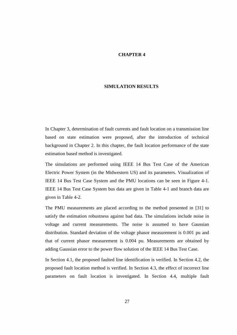
The simulations are performed using IEEE 14 Bus Test Case of the American
Electric Power System (in the Midwestern US) and its parameters. Visualization of
IEEE 14 Bus Test Case System and the PMU locations can be seen in Figure 4-1.
IEEE 14 Bus Test Case System bus data are given in Table 4-1 and branch data are
given in Table 4-2.
The PMU measurements are placed according to the method presented in [31] to
satisfy the estimation robustness against bad data. The simulations include noise in
voltage and current measurements. The noise is assumed to have Gaussian
distribution. Standard deviation of the voltage phasor measurement is 0.001 pu and
that of current phasor measurement is 0.004 pu. Measurements are obtained by
adding Gaussian error to the power flow solution of the IEEE 14 Bus Test Case.
In Section 4.1, the proposed faulted line identification is verified. In Section 4.2, the
proposed fault location method is verified. In Section 4.3, the effect of incorrect line
parameters on fault location is investigated. In Section 4.4, multiple fault
28
identification using the proposed method is examined. Finally, in Section 4.5, the
simulation results are discussed.
Figure 4-1 IEEE 14 Bus Test Case System

29
Table 4-1 Bus Data of IEEE 14 Bus Test Case System
Bus Load
[MW]
Load
[MVAR]
Generation
[MW]
Generation
[MVAR]
Shunt
Susceptance
B (per unit)
1 0 0 232.4 -.16.9 0
2 21.7 12.7 40 42.4 0
3 94.2 19 0 23.4 0
4 47.8 -3.9 0 0 0
5 7.6 1.6 0 0 0
6 11.2 7.5 0 12.2 0
7 0 0 0 0 0
8 0 0 0 17.4 0
9 29.5 16.6 0 0 0.19
10 9 5.8 0 0 0
11 3.5 1.8 0 0 0
12 6.1 1.6 0 0 0
13 13.5 5.8 0 0 0
14 14.9 5 0 0 0

30
Table 4-2 Branch Data of IEEE 14 Bus Test Case System
From
Bus
To Bus Branch
Resistance, R
(per unit)
Branch
Reactance, X
(per unit)
Line
Charging, B
(per unit)
Transformer
Tap Ratio
1 2 0.01938 0.05917 0.0528 0
1 5 0.05403 0.22304 0.0492 0
2 3 0.04699 0.19797 0.0438 0
2 4 0.05811 0.17632 0.034 0
2 5 0.05695 0.17388 0.0346 0
3 4 0.06701 0.17103 0.0128 0
4 5 0.01335 0.04211 0 0
4 7 0 0.20912 0 0.978
4 9 0 0.55618 0 0.969
5 6 0 0.25202 0 0.932
6 11 0.09498 0.1989 0 0
6 12 0.12291 0.25581 0 0
6 13 0.06615 0.13027 0 0
7 8 0 0.17615 0 0
7 9 0 0.11001 0 0
9 10 0.03181 0.0845 0 0
9 14 0.12711 0.27038 0 0
10 11 0.08205 0.19207 0 0
12 13 0.22092 0.19988 0 0
13 14 0.17093 0.34802 0 0

31
4.1 Verification of the Proposed Faulted Line Identification Method
This section aims to validate the proposed state estimation based faulted line
identification. For this purpose, first, state estimation for EMS use is performed.
Then, the bad data process, namely the largest normalized residuals test, is performed
and based on the test results, the lines associated with the identified bad
measurements are flagged as faulted lines. Note that, because of the model mismatch
due to the fault, the related current flow measurements will be identified as bad
measurements. Finally, iterative state estimation is performed to find fault location
on the identified line.
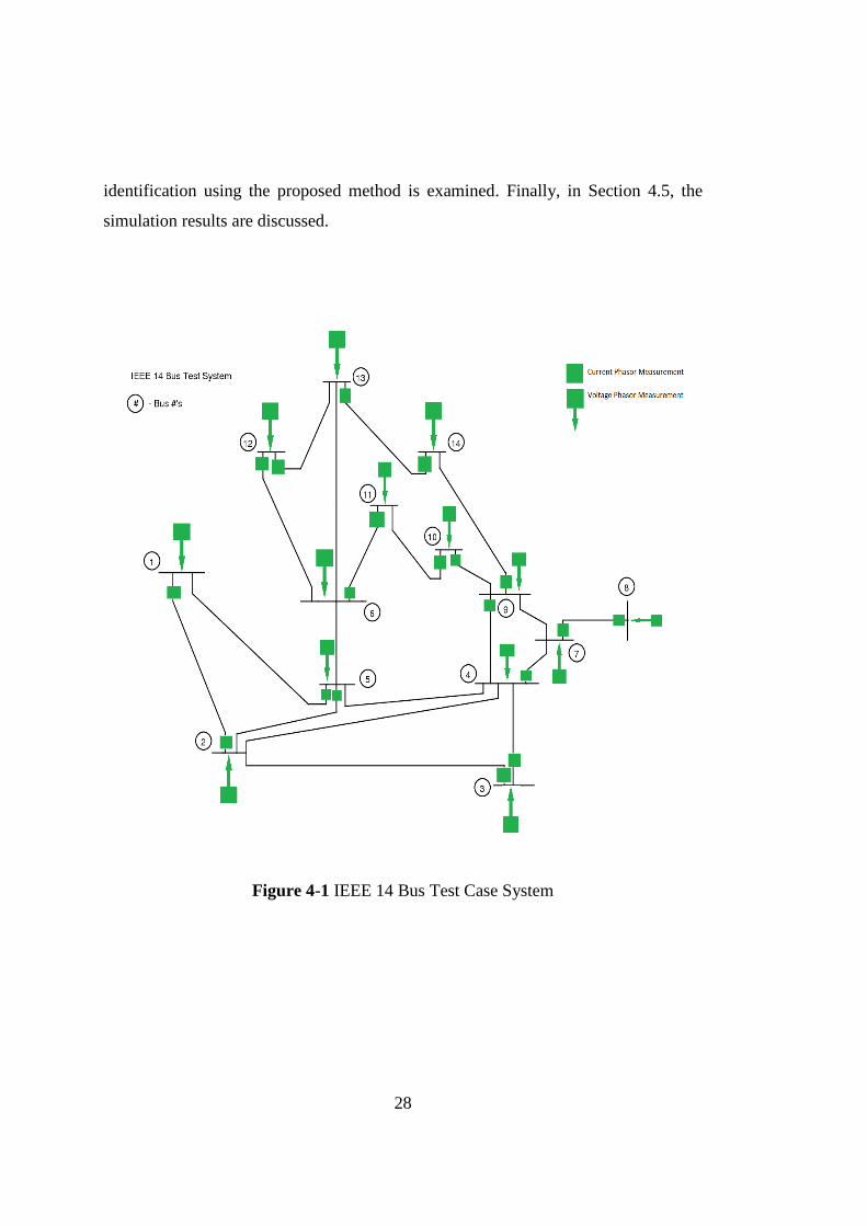
The number of Monte Carlo runs is 500 to validate the proposed state estimation
based faulted line identification. In each run, a three-phase to ground fault is located
to a random line, based on a pre-determined α and a given α0. The considered α and
α0 values are given in Table 4-3. The percentage Mean Absolute Error (pMAE) for
each group of α and α0 is calculated and presented in Table 4-3. Below is the
formulation of pMAE where N is the simulation run number.
∑|
|
(4.1)
Note that the “unfeasible” solution encountered in Table 4-3 satisfies the condition
(3.15), which means that using the given initial condition the feasible fault location
estimation cannot be reached. This problem can be overcome by resolving the
estimation problem with a different initial condition, α0. Considering that the
estimation problem solution is very fast, thanks to its small size, it can be concluded
that this extra re-estimation step will not affect the computational performance
significantly.
32
Table 4-3 pMAE for Different Fault Locations at Different Lines
pMAE α
0.05 0.5 0.95
α0
0.005 0.005 % 0 % 0 %
0.01 0.0034 % 0 % 0 %
0.02 0.0012 % 0% 0.0289 %
0.05 0 % 0 % unfeasible
0.99 0 % 0 % 0.0033 %
0.995 0 % 0 % 0.005 %
Figure 4-2 Error Between Estimated Location and Real Location for Different Lines
(α0: 0.005, α: 0.5)

33
Figure 4-3 Error Between Estimated Location and Real Location for Different Lines
(α0: 0.05, α: 0.95)
Once the simulation results are investigated, it is found that all the faulted lines are
identified correctly. However, the location of the fault on the identified line is not
estimated correctly for some simulations. Figure 4-2 depicts that estimated location
and real location is similar for all Monte Carlo results for the defined simulation
case. On the other hand, Figure 4-3 depicts that the error between estimated location
and real location has discrepancy for some of Monte Carlo results. This discrepancy
34
is caused by unfeasible solution, since (3.15) is satisfied. As explained previously,
this issue can be solved with an extra re-estimation step.
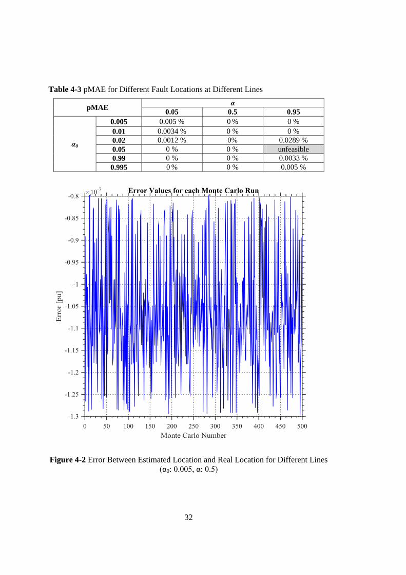
In addition to the simulations explained so far, the proposed method is also tested
with some realistic synthetic data obtained via DigSilent. A pre-determined line,
namely the branch between Bus-1 and Bus-2, is assumed as faulted. In DigSilent,
ANSI based short circuit (three-phase to ground) analysis is performed for the IEEE-
14 bus system. In Figure 4-4, a sample screenshot of IEEE-14 bus system in
DigSilent can be seen.
Figure 4-4 A Sample Screenshot of DigSilent while Short Circuit Analysis

35
Table 4-4 DigSilent Short Circuit Simulation Results for Different α Values
I1f I2f
Magnitude
[A]
Phase
[degree]
Magnitude
[A]
Phase
[degree]
α
0.1 9143 90.65 7220 92.33
0.5 8054 90.95 8304 91.83
0.7 7511 91.13 8849 91.62
DigSilent Short Circuit simulation results can be observed in Table 4-4.
Using the data in Table 4-4, the algorithm is run 100 times for each pre-determined α
(0.1, 0.5 and 0.7) and a given α0 (0.005). The percentage Mean Absolute Error
(pMAE) for each α is calculated and presented in Table 4-5.
Table 4-5 pMAE for a Given Fault Locations using DigSilent Data
α0 = 0.005 pMAE
α
0.1 0.072 %
0.5 0.063 %
0.7 0.056 %
Figure 4-5 shows the error between the estimated location and the real location, and
depicts that this error is negligible for all selected α values.

36
Figure 4-5 Performance of the Algorithm with DigSilent Data for Fault Between
Bus-1 and Bus-2
The same approach is also conducted for the line between Bus-7 and Bus-8. The
simulation results can be observed in Table 4-6.
Table 4-6 DigSilent Short Circuit Simulation Results for Different α Values
I1f I2f
Magnitude
[A]
Phase
[degree]
Magnitude
[A]
Phase
[degree]
α
0.1 9143 90.65 7220 92.33
0.5 8054 90.95 8304 91.83
0.7 7511 91.13 8849 91.62

37
The percentage Mean Absolute Error (pMAE) for each α is calculated and presented
in Table 4-7.
Table 4-7 pMAE for a Given Fault Locations using DigSilent Data
α0 = 0.005 pMAE
α
0.1 0.0183 %
0.5 0.0181 %
0.7 0.0186 %
The performance of the algorithm with DigSilent data for fault between Bus-7 and
Bus-8 can be seen in Figure 4-6. Figure 4-6 depicts that the error between estimated
location and real location is negligible for all selected α.
Figure 4-6 Performance of the Algorithm with DigSilent Data for Fault Between
Bus-7 and Bus-8

38
4.2 Verification of the Proposed Fault Location Method
In this simulation, a pre-determined line, namely the one between the Bus-1 and Bus-
2, is selected as the faulted line (three-phase to ground fault). Then Monte-Carlo
simulations are run changing α randomly. This study is repeated 500 times for each
α0, which are defined in Table 4-8. The pMAE of the estimation values of α in all
runs for different initial conditions are presented in Table 4-8. As seen in Table 4-8,
the proposed method successfully locates the fault at a given line.
Table 4-8 pMAE for Different Fault Location at a Given Line
α0 pMAE
0.005 0.1515 %
0.01 0.0355 %
0.02 0.0270 %
0.05 0.0242 %
0.99 0.0258 %
0.995 0.1589 %
Note that pMAE in Table 4-8 is calculated with respect to converged solutions.
Diverged solutions are disregarded, assuming that they can be corrected by changing
the initial condition. Errors for different fault location at a given line for each α0 can
be observed from Figure 4-7 through Figure 4-12.

39
Figure 4-7 Error Between Estimated Location and Real Location for α0 = 0.005

40
Figure 4-8 Error Between Estimated Location and Real Location for α0 = 0.01

41
Figure 4-9 Error Between Estimated Location and Real Location for α0 = 0.02
42
Figure 4-10 Error Between Estimated Location and Real Location for α0 = 0.05

43
Figure 4-11 Error Between Estimated Location and Real Location for α0 = 0.99
44
Figure 4-12 Error Between Estimated Location and Real Location for α0 = 0.995
Figure 4-7, Figure 4-8, Figure 4-9, Figure 4-10, Figure 4-11 and Figure 4-12 consist
of two parts, namely, Part-A and Part-B. Part-A demonstrates the difference (error)
between estimated location and real location of the fault for each Monte Carlo run.
Part-B demonstrates the actual α values for the unfeasible solutions. Part-B of Figure
4-7, Figure 4-8, Figure 4-9, Figure 4-10, Figure 4-11 and Figure 4-12 depict that
unfeasible solutions satisfies the condition (3.15) and (3.16). Since α0 value is

45
selected as too close to 0 or too close to 1, unfeasible solutions indicate that the fault
is located either at sending or receiving end.
Figure 4-13 Error Between Estimated Location and Real Location for varied α0
Finally in this section, it is shown that using a different α0 will enable convergence to
the feasible solution. For this purpose, a constant α value, 0.9992, is used instead of
changing it randomly. In the first 100 Monte Carlo runs, the value of α0 changes
from 0.0001 to 0.01 with the step increase of 0.0001 and in the last 100 Monte Carlo

46
run, the value of α0 changes from 0.99 to 0.9999 with the step increase of 0.0001.
Figure 4-13 shows that after 169th
Monte Carlo run whose corresponding α0 value is
0.9968, the fault location problem is solved successfully. The pMAE is found to be
0.0309%. However, before the 168th
Monte Carlo run, the solution is unfeasible. This
result shows that, once the unfeasible solution is encountered, a different α0 should be
employed and estimation should be re-performed. As mentioned formerly, thanks to
the small size of the estimation problem, this extra step will not bring a significant
computational load.
4.3 Effect of Incorrect Line Parameters on the Proposed Method
Due to the varying weather conditions, the line parameters are subject to change.
This section aims to validate even in the presence of incorrect line parameters, the
proposed method is capable of locating faults correctly. In order to have such
robustness against the incorrect line parameters, the problem formulation should be
modified.
The equations (4.2) and (4.3) can be derived using (3.10) and (3.11) respectively.
(4.2)
(4.3)
where Vi, Vj and Vf are the voltage phasors at Bus-i, Bus-j and the fault location,
respectively. Fault current flowing through Bus-i is represented by Ifi, while fault
current flowing through Bus-j is represented by Ifj. Z represents the series impedance
of the line between buses i and j, and bii and bjj represent the line charging
susceptances at Bus-i and Bus-j, respectively. Finally, α shows the ratio of the
distance of the fault to Bus-i to the total length of the faulted line.
Vf is calculated for each equations, (4.2) and (4.3), shown in (4.4) and (4.5).
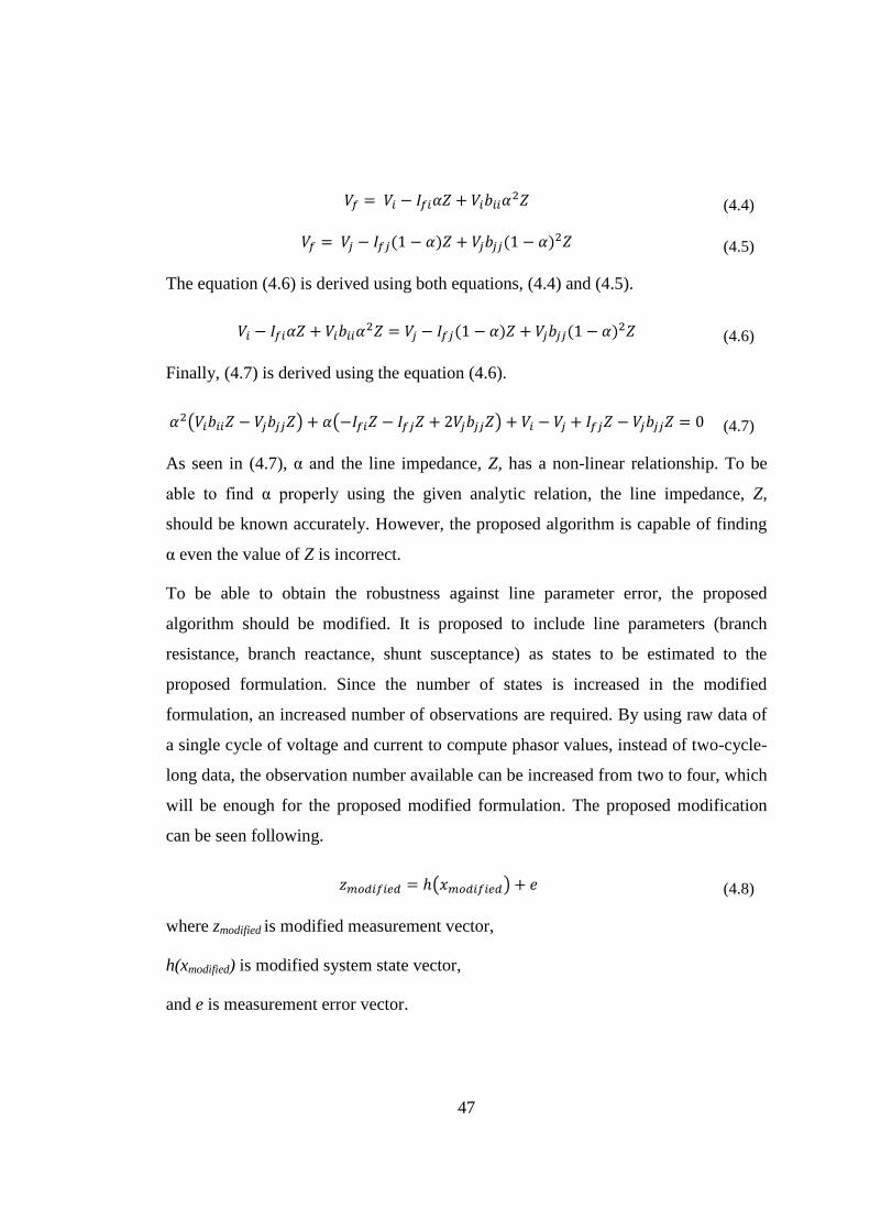
47
(4.4)
(4.5)
The equation (4.6) is derived using both equations, (4.4) and (4.5).
(4.6)
Finally, (4.7) is derived using the equation (4.6).
( ) ( ) (4.7)
As seen in (4.7), α and the line impedance, Z, has a non-linear relationship. To be
able to find α properly using the given analytic relation, the line impedance, Z,
should be known accurately. However, the proposed algorithm is capable of finding
α even the value of Z is incorrect.
To be able to obtain the robustness against line parameter error, the proposed
algorithm should be modified. It is proposed to include line parameters (branch
resistance, branch reactance, shunt susceptance) as states to be estimated to the
proposed formulation. Since the number of states is increased in the modified
formulation, an increased number of observations are required. By using raw data of
a single cycle of voltage and current to compute phasor values, instead of two-cycle-
long data, the observation number available can be increased from two to four, which
will be enough for the proposed modified formulation. The proposed modification
can be seen following.
( ) (4.8)
where zmodified is modified measurement vector,
h(xmodified) is modified system state vector,
and e is measurement error vector.

48
[
]
(4.9)
where,
- mr
fV
,is the real part of the voltage phasor at the fault location at time instant-
m,
- mi
fV
,is the imaginary part of the voltage phasor at the fault location at time
instant-m,
- α1 is the ratio of the distance of the fault to sending end bus to the total length
of the faulted line
- α2 is the ratio of the distance of the fault to receiving end bus to the total
length of the faulted line
- gij is the shunt conductance between sending end bus and receiving end bus,
- bij is the shunt susceptance between sending end bus and receiving end bus,
- bii is the half of the total line charging between sending end bus and receiving
end bus,
- Vsr,m
is the real part of the system state voltage of sending end bus at time
instant-m,
- Vrr,m
is the real part of the system state voltage of receiving end bus at time
instant-m,
- Vsi,m
is the imaginary part of the system state voltage of sending end bus at
time instant-m,
49
- Vsi,m
is the imaginary part of the system state voltage of receiving end bus at
time instant-m,
[
]
(4.10)
where,
- Isr,m
is the real part of the measured current of sending end of the faulted line
at time instant-m,
- Irr,m
is the real part of the measured current of receiving end of the faulted line
at time instant-m,
- Isi,m
is the imaginary part of the measured current of sending end of the
faulted line at time instant-m,
- Iri,m
is the imaginary part of the measured current of receiving end of the
faulted line at time instant-m,
- α1 is the ratio of the distance of the fault to sending end bus to the total length
of the faulted line
- α2 is the ratio of the distance of the fault to receiving end bus to the total
length of the faulted line
- Vsr,m
is the real part of the system sending end bus voltage at time instant-m,
- Vrr,m
is the real part of the system receiving end bus voltage at time instant-m,
- Vsi,m
is the imaginary part of the sending end bus voltage at time instant-m,

50
- Vsi,m
is the imaginary part of the receiving end bus voltage at time instant-m,
The simulations are repeated 200 times by changing α randomly. In each run of
algorithm, a three-phase to ground fault is located between the Bus-1 and Bus-2. The
faulted line impedance, given in Table 4-2, is multiplied by a coefficient. The
coefficient is chosen as 2 for the half of the Monte Carlo simulations and for the rest
of the Monte Carlo simulations it is chosen as 0.5. The pMAE of the estimation
values of α in all runs for different initial conditions are presented in Table 4-9.
Table 4-9 pMAE for Different Fault Location at a Given Line with incorrect
impedance
α0 pMAE
0.005 0.1473 %
0.01 0.0106 %
0.02 0.0339 %
0.05 0.0138 %
0.99 0.053 %
0.995 0.1541 %
The results in Table 4-9 are similar with the pMAEs of Table 4-8. This result
validates the proposed method is capable of locating faults correctly, even in the
presence of incorrect line parameters.
The performance of the algorithm for a fault between Bus-1 and Bus-2 can be seen in
Figure 4-14. Figure 4-14 shows the error between estimated location and real
location. All Monte Carlo runs are taken when the line parameters of the branch
between Bus-1 and Bus-2 are doubled.

51
Figure 4-14: Error Between Estimated Location and Real Location with Incorrect
Impedance
Figure 4-14 depicts that the estimated fault location is not affected under the
incorrect line parameters.
4.4 Effect of Multiple Faults on the Proposed Method
This section aims to validate fault location with proposed method when there are
multiple faults in the system. The faulted lines are selected between the Bus-1 and

52
Bus-2 and between Bus-6 and Bus-11. Then Monte-Carlo simulations are run 100
times by changing α of each faulted line randomly. The pMAE for each α is
calculated and presented in Table 4-10.
Table 4-10 pMAE for a Given Fault Locations
Faulted Line pMAE (α0 = 0.005)
Between Bus-1 and Bus-2 0.0109 %
Between Bus-6 and Bus-11 0.001 %
4.5 Discussion
The simulations were performed in MATLAB environment by following the steps
stated below.
The IEEE 14-bus system is employed.
Optimal PMU placement algorithm is run to be able to have an observable
system.
Power flow problem is solved to obtain the measurement set for the state
estimator.
Faulted line is found with state estimation and bad data process (Normalized
Residual Test).
Fault location is determined with WLS.
MAEs of estimated values of fault location are found with Monte Carlo
analysis.
Simulation results demonstrate that
The proposed method can identify faulted lines successfully.

53
The proposed approach can locate a fault on an identified faulted line
accurately.
Initial condition, α0, is critical because of the risk of unfeasible solution.
Using small α0 values can solve the unfeasible solution problem.
Small α0 values might increase the iteration of the solution.
When small size of the problem is considered, the increased number of
iterations will not create a significant change in the total solution time of the
problem.
Even the fault line impedance is incorrect, the proposed algorithm can handle
this situation and finds fault location accurately.
The proposed algorithm is capable of locating multiple faults.


55
CHAPTER 5
5. CONCLUSION
Fault location is especially important for the restoration of electrical power, which
will increase the reliability of the system and decrease the operational cost. The main
motivation of this thesis work was to locate a permanent fault with a technique based
on the well-known WLS state estimation method.
The method assumes that the considered system is observable solely by PMUs
considering their increasing number. The high refresh rate and time synchronization
of the PMU measurements is the reason of using those data for the proposed method.
Note that, the proposed method is applicable to any synchronized data set that may
be received from PMUs or power quality monitors. The contributions of the
proposed method can be listed as follows.
The state estimation based method uses multiple time scans to increase the
accuracy of the fault location, and to eliminate the measurement redundancy
problem.
The proposed faulted line identification is actually a part of conventional state
estimation, and hence will not bring any computational burden. Thanks to the
local problem formulation, the computational burden of the fault location on
a transmission line is negligible.

56
During simulations it was observed that the initial condition of the estimation
problem is critical, because of the risk of unfeasible solution. Therefore, it is
proposed to use small α0 values to initialize the problem. This choice might
increase the iterations of the solution, but considering the small size of the
problem, the increased number of iterations will not create a significant
change in the total solution time of the problem.
The proposed faulted line identification method is capable of identifying
multiple faulted lines in the system.
The proposed fault location method is capable of eliminating the effect of
incorrect line parameters, which brings robustness against the parameter
changes due to weather conditions.
In this thesis work, all relations are derived for three-phase to ground fault.
However, if a three-phase estimator is employed, the proposed fault location
method can be applied independent of the fault type.
In the future, it is aimed to apply the proposed method using real time
synchronized PMU measurements.

57
REFERENCES
[1] S. Santoso, A. Gaikwad and M. Patel, “Impedance-Based Fault Location in
Transmission Networks: Theory and Application,” IEEE Access, vol. 2, pp.
537-557, 2014.
[2] T. Takagi, Y. Yamakoshi, M. Yamaura, R. Kondow, and T. Matsushima,
“Development of a new type fault locator using the one-terminal voltage and
current data,” IEEE Trans. Power App. Syst., vol. PAS-101, no. 8, pp. 2892–
2898, Aug. 1982.
[3] L. Eriksson, M. M. Saha, and G. D. Rockefeller, “An accurate fault locator
with compensation for apparent reactance in the fault resistance resulting from
remore-end infeed,” IEEE Trans. Power App. Syst., vol. PAS-104, no. 2, pp.
423–436, Feb. 1985.
[4] T. Kawady and J. Stenzel, “A practical fault location approach for double
circuit transmission lines using single end data,” IEEE Trans. Power Del., vol.
18, no. 4, pp. 1166–1173, Oct. 2003.
[5] C. E. M. Pereira and L. C. Zanetta, Jr., “Fault location in transmission lines
using one-terminal postfault voltage data,” IEEE Trans. Power Del., vol. 19,
no. 2, pp. 570–575, Apr. 2004.
[6] M. Kezunovic and B. Perunicic, “Automated transmission line fault analysis
using synchronized sampling at two ends,” IEEE Trans. Power Syst., vol. 11,
no. 1, pp. 441–447, Feb. 1996.

58
[7] A. L. Dalcastagnê, S. N. Filho, H. H. Zürn, and R. Seara, “An iterative two-
terminal fault-location method based on unsynchronized phasors,” IEEE Trans.
Power Del., vol. 23, no. 4, pp. 2318–2329, Oct. 2008.
[8] Y. Liao and N. Kang, “Fault-location algorithms without utilizing line
parameters based on the distributed parameter line model,” IEEE Trans. Power
Del., vol. 24, no. 2, pp. 579–584, Apr. 2009.
[9] J. Izykowski, E. Rosolowski, P. Balcerek, M. Fulczyk, and M. M. Saha,
“Accurate noniterative fault location algorithm utilizing two-end
unsynchronized measurements,” IEEE Trans. Power Del., vol. 25, no. 1, pp.
72–80, Jan. 2010.
[10] C. A. Apostolopoulos and G. N. Korres, “A novel algorithm for locating faults
on transposed/untransposed transmission lines without utilizing line
parameters,” IEEE Trans. Power Del., vol. 25, no. 4, pp. 2328–2338, Oct.
2010.
[11] T. Nagasawa, M. Abe, N. Otsuzuki, T. Emura, Y. Jikihara, and M. Takeuchi,
“Development of a new fault location algorithm for multiterminal two parallel
transmission lines,” IEEE Trans. Power Del., vol. 7, no. 3, pp. 1516–1532, Jul.
1992.
[12] D. A. Tziouvaras, J. B. Roberts, and G. Benmouyal, “New multi-ended fault
location design for two- or three-terminal lines,” in Proc. 7th Int. Conf.
Develop. Power Syst. Protection, 2001, pp. 395–398.
[13] G. Manassero, E. C. Senger, R. M. Nakagomi, E. L. Pellini, and E. C. N.
Rodrigues, “Fault-location system for multiterminal transmission lines,” IEEE
Trans. Power Del., vol. 25, no. 3, pp. 1418–1426, Jul. 2010.

59
[14] T. Funabashi, H. Otoguro, Y. Mizuma, L. Dube, and A. Ametani, “Digital fault
location for parallel double-circuit multi-terminal transmission lines,” IEEE
Trans. Power Del., vol. 15, no. 2, pp. 531–537, Apr. 2000.
[15] S. M. Brahma, “Fault location scheme for a multi-terminal transmission line
using synchronized voltage measurements,” IEEE Trans. Power Del., vol. 20,
no. 2, pp. 1325–1331, Apr. 2005.
[16] C.-W. Liu, K.-P. Lien, C.-S. Chen, and J.-A. Jiang, “A universal fault location
technique for N-terminal transmission lines,” IEEE Trans. Power Del., vol. 23,
no. 3, pp. 1366–1373, Jul. 2008.
[17] S. Rajendra and P. G. McLaren, “Travelling-wave techniques applied to the
protection of teed circuits: Multi-phase/multi-circuit system,” IEEE Trans.
Power App. Syst., vol. PAS-104, no. 12, pp. 3551–3557, Dec. 1985.
[18] A. O. Ibe and B. J. Cory, “A travelling wave-based fault locator for two- and
three-terminal networks,” IEEE Trans. Power Del., vol. 1, no. 2, pp. 283–288,
Apr. 1986.
[19] F. H. Magnago and A. Abur, “Fault location using wavelets,” IEEE Trans.
Power Del., vol. 13, no. 4, pp. 1475–1480, Oct. 1998.
[20] C. Y. Evrenosoglu and A. Abur, “Travelling wave based fault location for teed
circuits,” IEEE Trans. Power Del., vol. 20, no. 2, pp. 1115–1121, Apr. 2005.
[21] D. Spoor and J. G. Zhu, “Improved single-ended traveling-wave fault location
algorithm based on experience with conventional substation transducers,”
IEEE Trans. Power Del., vol. 21, no. 3, pp. 1714–1720, Jul. 2006.
[22] P. Jafarian and M. Sanaye-Pasand, “A traveling-wave-based protection
technique using wavelet/PCA analysis,” IEEE Trans. Power Del., vol. 25, no.
2, pp. 588–599, Apr. 2010.

60
[23] M. Korkali and A. Abur, “Fault location in meshed power networks using
synchronized measurements,” in Proc. North American Power Symp., Sep.
2010.
[24] M. Korkali, H. Lev-Ari and A. Abur, “Traveling-Wave-Based Fault-Location
Technique for Transmission Grids Via Wide-Area Synchronized Voltage
Measurements,” IEEE Trans. Power Sys., vol. 27, no. 2, pp. 1003–1011, May
2012.
[25] Volkan Özdemir, “A Local Parameter Estimator Based on Robust LAV
Estimation,” MS Thesis, Middle East Technical University, 2015.
[26] A. G. Phadke, J. S. Thorp, “Synchronized Phasor Measurements and Their
Applications”, book, Springer, 2008.
[27] A. Abur and A. Gomez-Exposito, “Power System State Estimation: Theory and
Implementation”, Marcel Dekker, 2004.
[28] A. Akyel, “Detemination of Dynamic Problems Associated with the Wind
Power Plants in Turkish Transmission System,” MS Thesis, Middle East
Technical University, 2015.
[29] M. Shiroei, S. Daniar and M. Akhbari, “A new algorithm for fault location on
transmission lines”, in proc. IEEE Power & Energy Society General Meeting,
2009, pp. 1-5.
[30] A. C. Aitken, “On Least Squares and Linear Combinations of Observations”,
Proc. Royal Society of Edinburg, 1935, vol. 35, pp. 42-48.
[31] M. Göl, A. Abur. “Optimal PMU Placement for State Estimation Robustness,”
IEEE Innovative Smart Grid Technologies (ISGT) Europe, Oct. 2014.
[32] A. Monticelli and A. Garcia, “Reliable Bad Data Processing for Real-Time
State Estimation,” IEEE Transactions on Power Apparatus and Systems, Vol.
PAS-102, No. 5, May 1983, pp. 1126-1139.