Stat 512

Day 9: Confidence Intervals (Ch 5)

Open Stat 512 Java Applets page

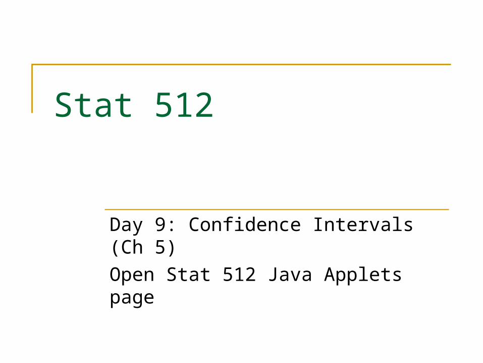
Last Time – Tests of Significance0. Define the parameter of interest1. Check technical conditions2. State competing null and alternative hypotheses

about the population parameter of interest (in symbols and in words)

H0: parameter = value

Ha: parameter value

parameter = population mean, ; population proportion,

Statement of research

conjecture

PP

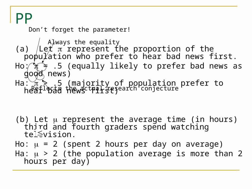
(a) Let represent the proportion of the population who prefer to hear bad news first.

Ho: = .5 (equally likely to prefer bad news as good news)Ha: > .5 (majority of population prefer to hear bad news

first)

(b) Let represent the average time (in hours) third and fourth graders spend watching television.

Ho: = 2 (spent 2 hours per day on average)Ha: > 2 (the population average is more than 2 hours per

day)

Don’t forget the parameter!

Always the equality

Reflects the actual research conjecture

PP

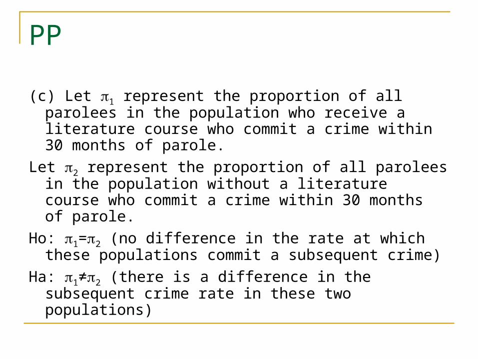
(c) Let 1 represent the proportion of all parolees in the population who receive a literature course who commit a crime within 30 months of parole.

Let 2 represent the proportion of all parolees in the population without a literature course who commit a crime within 30 months of parole.

Ho: 1=2 (no difference in the rate at which these populations commit a subsequent crime)

Ha: 1≠2 (there is a difference in the subsequent crime rate in these two populations)

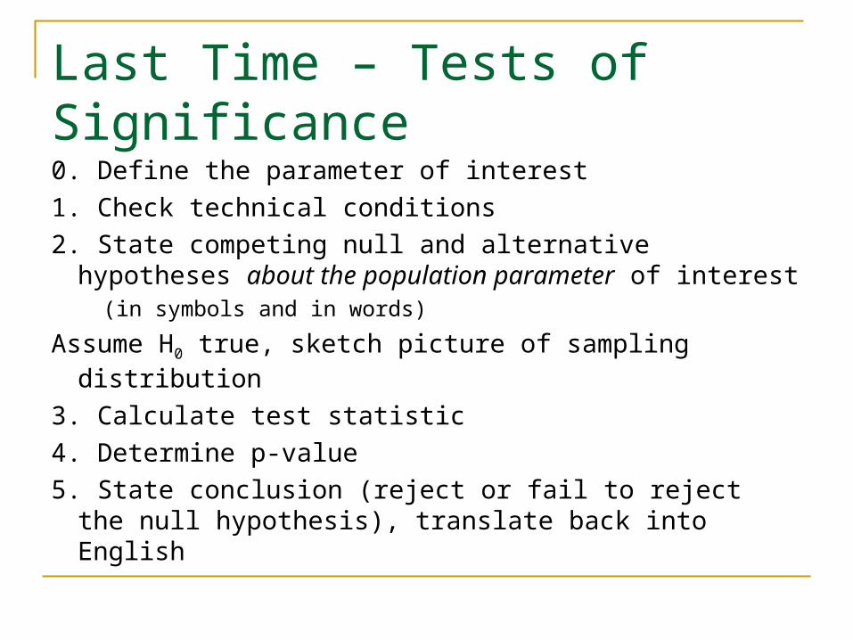
Last Time – Tests of Significance0. Define the parameter of interest

1. Check technical conditions

2. State competing null and alternative hypotheses about the population parameter of interest

(in symbols and in words)

Assume H0 true, sketch picture of sampling distribution

3. Calculate test statistic

4. Determine p-value

5. State conclusion (reject or fail to reject the null hypothesis), translate back into English

Interpreting p-value

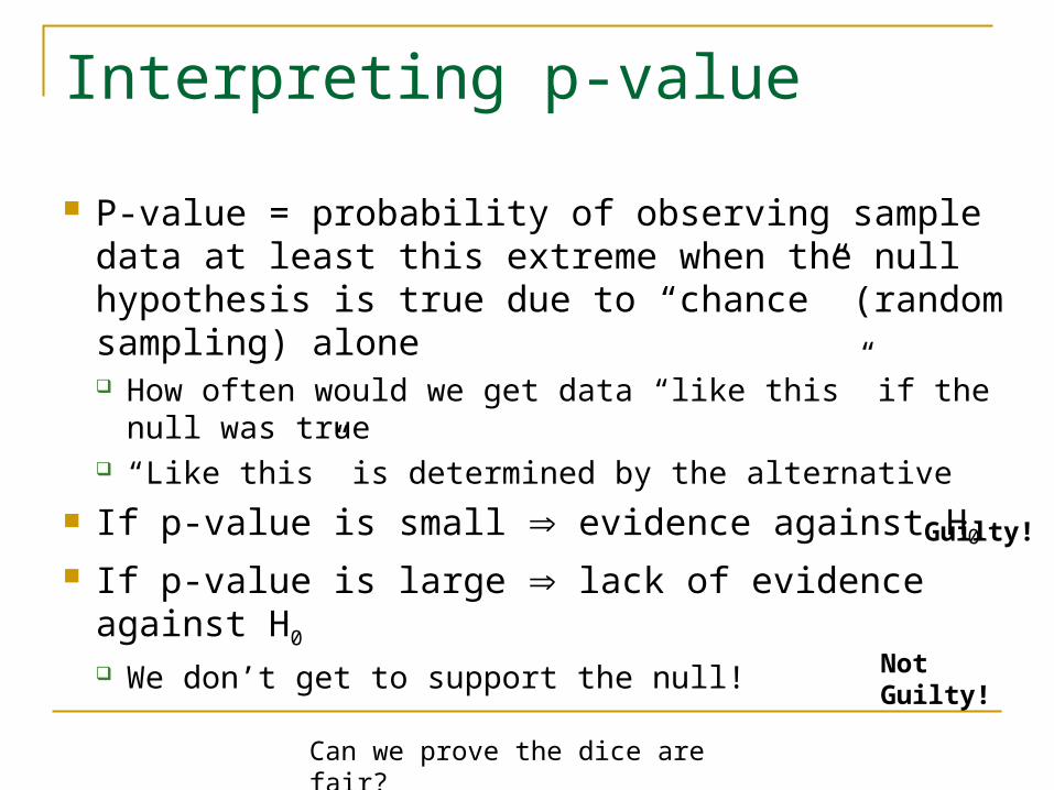
P-value = probability of observing sample data at least this extreme when the null hypothesis is true due to “chance” (random sampling) alone How often would we get data “like this” if the null was

true “Like this” is determined by the alternative

If p-value is small evidence against H0

If p-value is large lack of evidence against H0

We don’t get to support the null!

Guilty!

Not Guilty!

Can we prove the dice are fair?

Example?

I love all chocolate ice cream Have yet to find a choc ice cream don’t like…

Data are behaving as expected based on that initial belief… have no reason to doubt it…

What if I find one that I don’t like? Specify alternative as what hoping to show…

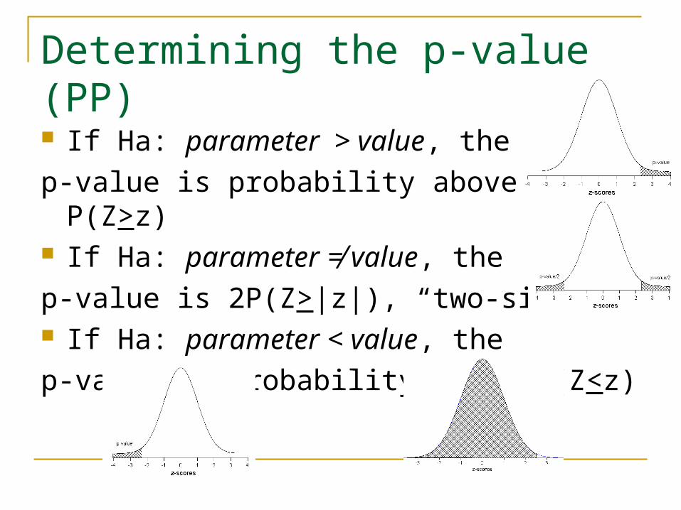
Determining the p-value (PP)

If Ha: parameter> value, the

p-value is probability above, P(Z>z) If Ha: parameter ≠ value, the

p-value is 2P(Z>|z|), “two-sided” If Ha: parameter < value, the

p-value is probability below P(Z<z)

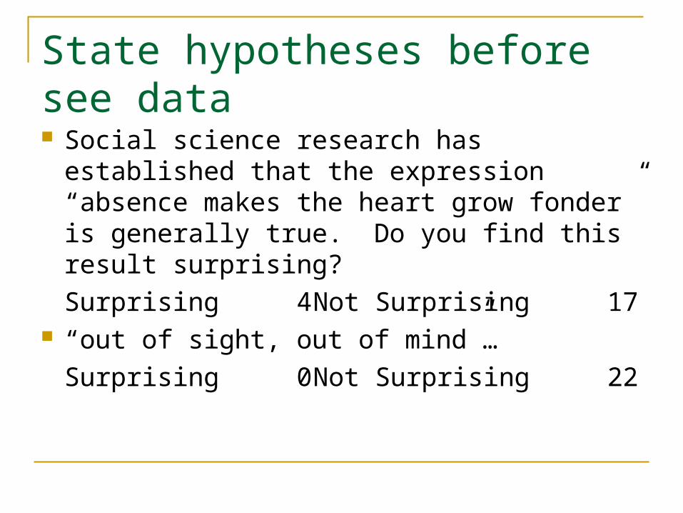
State hypotheses before see data Social science research has established that

the expression “absence makes the heart grow fonder” is generally true. Do you find this result surprising?

Surprising 4 Not Surprising 17 “out of sight, out of mind”…

Surprising 0 Not Surprising 22

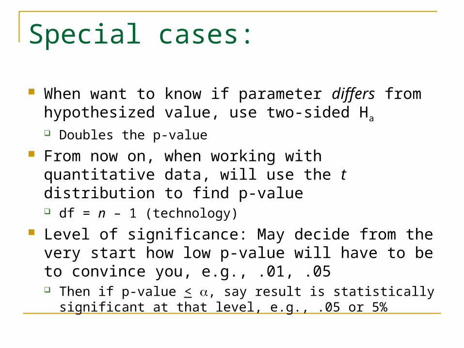
Special cases:

When want to know if parameter differs from hypothesized value, use two-sided Ha

Doubles the p-value From now on, when working with quantitative data,

will use the t distribution to find p-value df = n – 1 (technology)

Level of significance: May decide from the very start how low p-value will have to be to convince you, e.g., .01, .05 Then if p-value < , say result is statistically significant at

that level, e.g., .05 or 5%

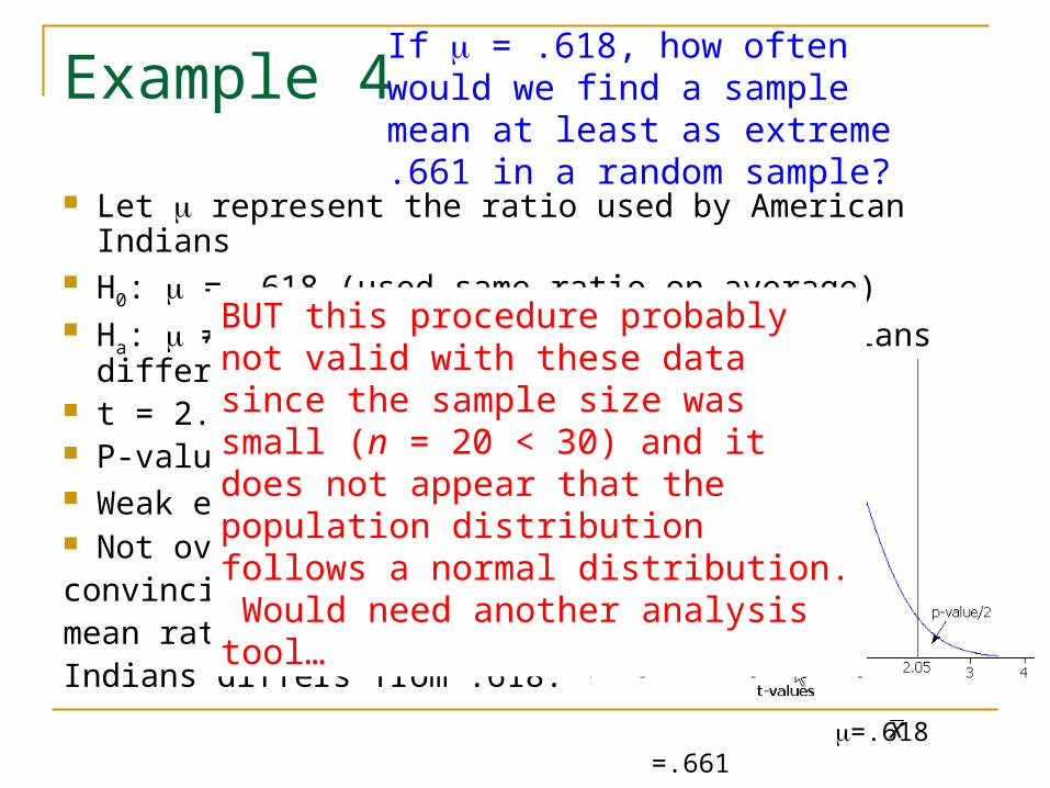
Example 4

Let represent the ratio used by American Indians H0: = .618 (used same ratio on average) Ha: ≠ .618 (ratio used by American Indians differs) t = 2.05 with df = 19 P-value = .054 Weak evidence against H0

Not overwhelmingly convincing that the mean ratio used by American Indians differs from .618.

BUT this procedure probably not valid with these data since the sample size was small (n = 20 < 30) and it does not appear that the population distribution follows a normal distribution. Would need another analysis tool…

If = .618, how often would we find a sample mean at least as extreme .661 in a random sample?

=.618 =.661 x

The next question:

People turn to the right more than half the time… the average healthy temperature of an American adult is not 98.6oF… less than 51% of Brown athletes are women…

Tests of significance have only told us what the parameter value is not, well what is it?

Example 1: Kissing the Right Way If more than half the population turns to the

right, how often is it? 2/3 of the time? ¾ of the time? 70% of the time?

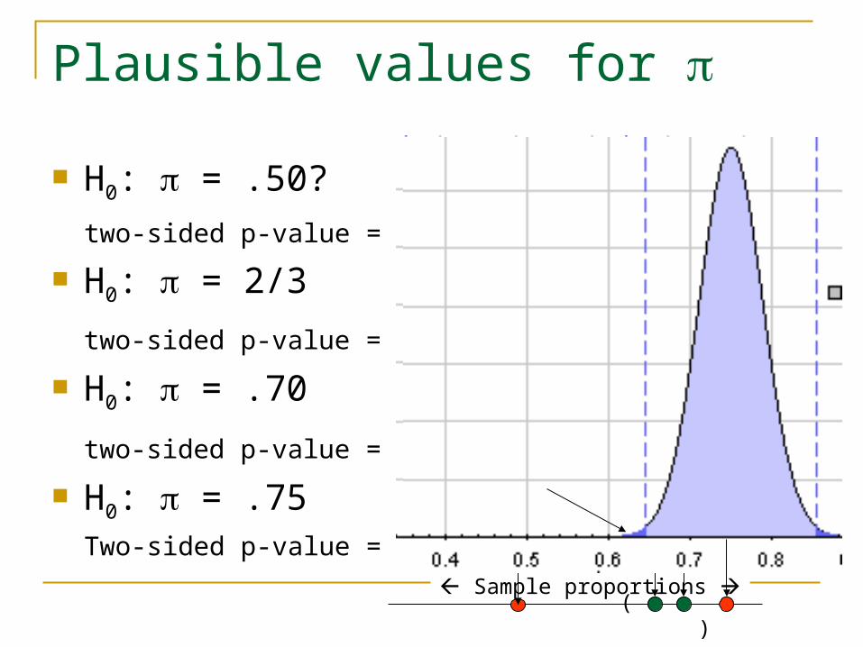
Plausible values for

H0: = .50?

two-sided p-value = .0012

H0: = 2/3

two-sided p-value = .5538

H0: = .70

two-sided p-value = .1814

H0: = .75Two-sided p-value = .0069

Sample proportions ( )

Observed sampleproportion

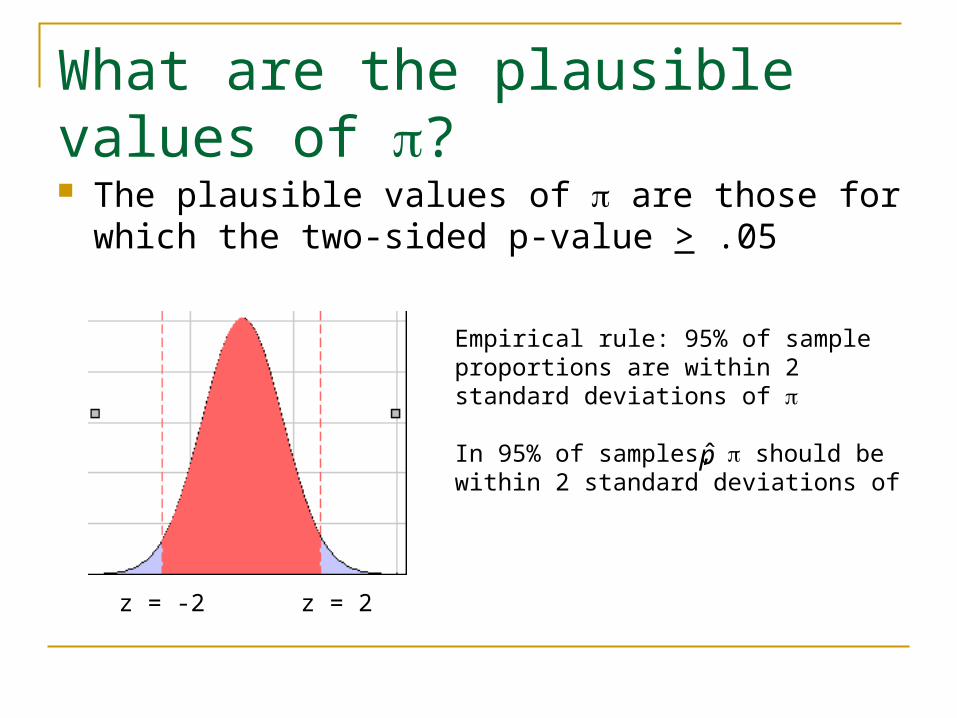
What are the plausible values of ? The plausible values of are those for which the

two-sided p-value > .05

z = -2 z = 2

Empirical rule: 95% of sample proportions are within 2 standard deviations of

In 95% of samples, should be within 2 standard deviations of p̂

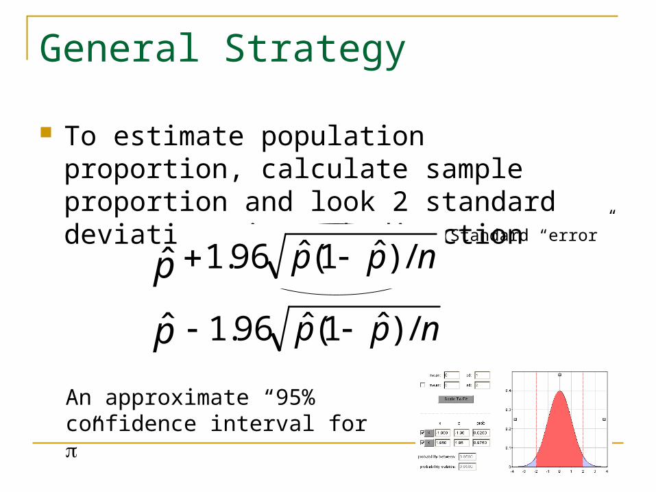
General Strategy

To estimate population proportion, calculate sample proportion and look 2 standard deviations in each direction

p̂

p̂

n/)1(2

n/)1(2

npp /)ˆ1(ˆ2

npp /)ˆ1(ˆ2

Standard “error”

npp /)ˆ1(ˆ96.1

npp /)ˆ1(ˆ96.1

An approximate “95% confidence interval for ”

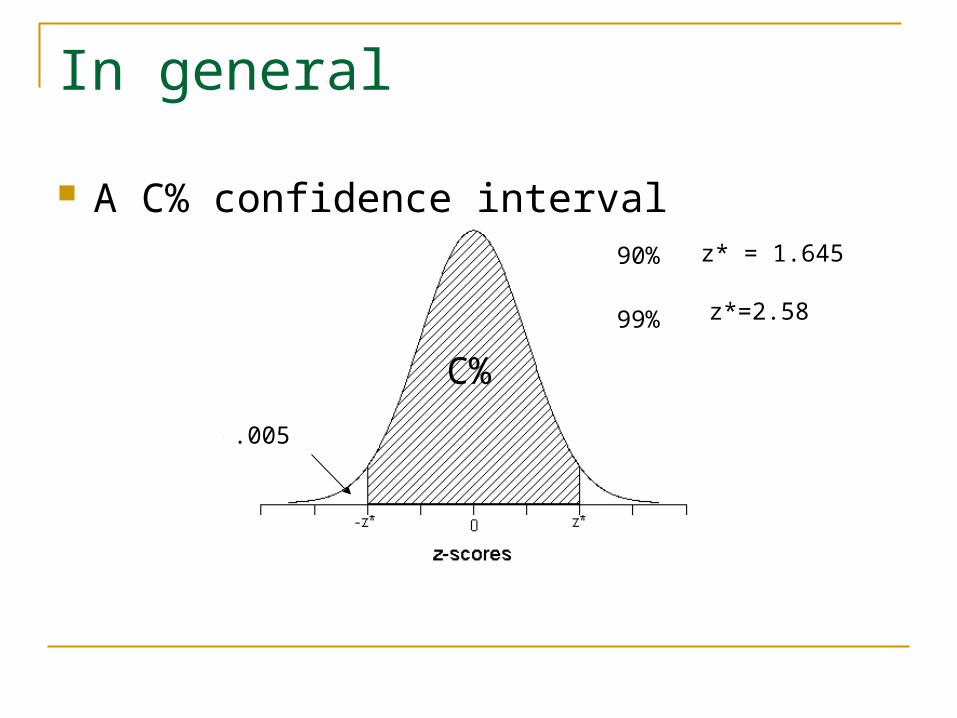
In general

A C% confidence interval

(100-C)/2

90%

.05

z* = 1.645

99%

.005

z*=2.58

C%

Example 2: NCAA Gambling

= proportion of all male NCAA athletes who participate in some type of gambling behavior

= .634 .634 + 1.96 sqrt(.634(1-.634)/12651) .634 + .008 We are 95% confident that , the probability that an

NCAA Div I athlete gambles, is between .626 and .642.

Between 62.6% and 64.2% of Div I athlete gamble.

p̂

Example 3: Body Temperatures Let = average body temperature of a

healthy adult We are 95% confident that the mean body

temperature of healthy adults is between 98.07oF and 98.33oF (assuming this sample was representative)

What if we only asked women?

Example 4: NCAA Gambling cont What sample size is needed if we want the

margin of error to be .01, with 95% confidence With qualitative data, if don’t have a prior guess

for , then use .5 – this guarantees margin of error is not larger…

If n is non-integer, always round up to the nearest integer

Example 5: What do we mean by “confidence”? Determine confidence interval using your

sample proportion of orange candies… Did everyone obtain the same interval? Will everyone’s interval capture ?

Interpretation of confidence

What is the reliability of this procedure… Assuming the Central Limit Theorem applies, how

often will a C% confidence interval succeed in capturing the population parameter

To explore this, have to pretend we know the population parameter

Interpretation of confidence

What if I put all of these confidence intervals into a bag and randomly selected one?

The confidence level is a probability statement about the method, not individual intervals If we had millions of intervals… Sample size?

For Next Time

Finish “surveys” on BB PP using applet HW 5

Problems 2 and 3… Review sheet and suggested problems have

been posted on line