STAT 400 Exam I More Discrete RVs Fall 2017

Practice 1. Let X be a discrete random variable with p.m.f.

p ( k ) = k

c

43

⋅ , k = 5, 6, 7, 8, … .

a) Find the value of c that makes this is a valid probability distribution.

b) Find P ( X is even ).

c) Find the moment-generating function of X, M X ( t ). For which values of t does it exist?

d) Find E ( X ). 2. Suppose a discrete random variable X has the following probability distribution:

P( X = k ) = ( )!

2lnk

k, k = 1, 2, 3, … .

a) Verify that this is a valid probability distribution.

b) Find µ X = E( X ) by finding the sum of the infinite series. c) Find the moment-generating function of X, M X ( t ).

d) Use M X ( t ) to find µ X = E( X ).

e) Find µ X = E( X ) by comparing it to the expected value of a Poisson random

variable with mean λ = ln 2. “Hint”: The answers to (b), (d), and (e) should be the same.

f) Find σ X2 = Var( X ).

3. The manufacturer of a price-reading scanner claims that the probability that the scanner will misread a price is 0.01. Shortly after one of the scanners was installed in a supermarket, the store manager tested the performance of the scanner. Assume that the outcome of each scan is independent of the others. a) Assuming that their claim is correct, what is the probability that the first time the scanner misreads a price will be on the seventh scan? b) Find the probability that the second error will be on the twenty fifth scan? c) Find the probability that the third error will be on the twenty fifth scan? d) Suppose 25 prices were read. Find the probability of more than one error. e) Suppose 25 prices were read. Find the probability of exactly one error. f) Suppose 25 prices were read. Find the probability of exactly two errors. 4. A purchasing agent is considering an acceptance plan for incoming lots of some manufactured product. The plan calls for taking a random sample of 20 items with replacement from each lot. If there is at most one defective in the sample, the lot is accepted; otherwise the lot is rejected. Find the probability of accepting the lot, if the defective rate is … a) 1%, b) 5%, c) 10%. 5. A credit card company sends a special pre-approved low-interest application form to a random sample of 25 individuals. Past experience indicates that about 10% of the people who receive such an application eventually reply. Let X denote the number of replies received in this sample of 25 individuals. a) Find the probability of receiving at most 3 replies. b) Find the probability of receiving exactly 3 replies. c) Find the probability of receiving at least 3 replies. d) Find the probability of receiving between 2 and 4 (both inclusive) replies.

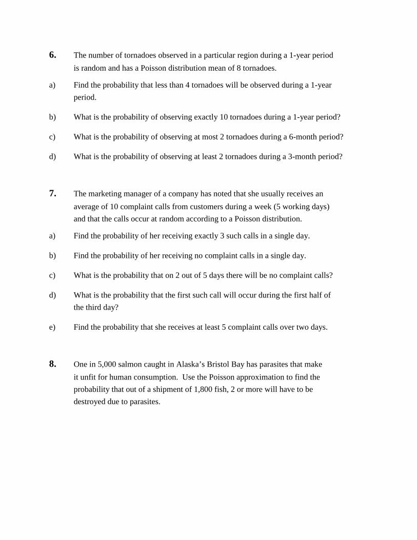
6. The number of tornadoes observed in a particular region during a 1-year period is random and has a Poisson distribution mean of 8 tornadoes. a) Find the probability that less than 4 tornadoes will be observed during a 1-year period. b) What is the probability of observing exactly 10 tornadoes during a 1-year period? c) What is the probability of observing at most 2 tornadoes during a 6-month period? d) What is the probability of observing at least 2 tornadoes during a 3-month period? 7. The marketing manager of a company has noted that she usually receives an average of 10 complaint calls from customers during a week (5 working days) and that the calls occur at random according to a Poisson distribution. a) Find the probability of her receiving exactly 3 such calls in a single day. b) Find the probability of her receiving no complaint calls in a single day. c) What is the probability that on 2 out of 5 days there will be no complaint calls? d) What is the probability that the first such call will occur during the first half of the third day? e) Find the probability that she receives at least 5 complaint calls over two days. 8. One in 5,000 salmon caught in Alaska’s Bristol Bay has parasites that make it unfit for human consumption. Use the Poisson approximation to find the probability that out of a shipment of 1,800 fish, 2 or more will have to be destroyed due to parasites.

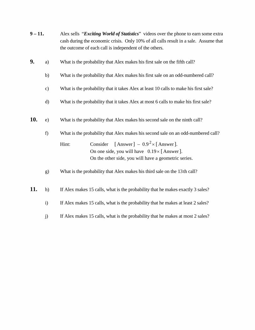
9 – 11. Alex sells “Exciting World of Statistics” videos over the phone to earn some extra cash during the economic crisis. Only 10% of all calls result in a sale. Assume that the outcome of each call is independent of the others.

9. a) What is the probability that Alex makes his first sale on the fifth call? b) What is the probability that Alex makes his first sale on an odd-numbered call? c) What is the probability that it takes Alex at least 10 calls to make his first sale? d) What is the probability that it takes Alex at most 6 calls to make his first sale? 10. e) What is the probability that Alex makes his second sale on the ninth call? f) What is the probability that Alex makes his second sale on an odd-numbered call? Hint: Consider [ Answer ] – 0.9

2 × [ Answer ]. On one side, you will have 0.19 × [ Answer ]. On the other side, you will have a geometric series. g) What is the probability that Alex makes his third sale on the 13 th call? 11. h) If Alex makes 15 calls, what is the probability that he makes exactly 3 sales? i) If Alex makes 15 calls, what is the probability that he makes at least 2 sales? j) If Alex makes 15 calls, what is the probability that he makes at most 2 sales?

12. a) Let X have a Poisson distribution with variance of 3. Find P ( X = 2 ). b) If X has a Poisson distribution such that 3 P ( X = 1 ) = P ( X = 2 ), find P ( X = 4 ). 13. Suppose the number of air bubbles in window glass has a Poisson distribution, with an average of 0.3 air bubbles per square foot. In a 4 ' by 3 ' window, find the probability that there are … a) … exactly 5 air bubbles. b) … at least 5 air bubbles. From the textbook: Ninth Eighth Seventh 2.4-10 2.4-12 2.4.14 2.4-15 2.4-18 2.4.20 2.5-3 2.5-10 2.5.10 2.6-8 2.6-8 2.6.8

1. Let X be a discrete random variable with p.m.f.

p ( k ) = k

c

43

⋅ , k = 5, 6, 7, 8, … .

a) Find the value of c that makes this is a valid probability distribution.

Must have ( )∑x

xp all

= 1. ⇒ ∑∞

=5

43

k

kc = ∑

∞

=5

43

k

kc = 1.

∑∞

=5

43

k

k =

basetermfirst

−1 =

431

43 5

−

=

41

1024243

= 256243 .

OR

∑∞

=5

43

k

k =

25681

6427

169

431

43

0

−−−−−∞

∑

=k

k

= 25681

256108

256144

256192

256256

431

1−−−−−

− =

2567814 − =

2567811024 − =

256243 .

⇒ c = 243256 =

5

4

3

4 .

b) Find P ( X is even ). P ( X is even ) = p ( 6 ) + p ( 8 ) + p ( 10 ) + p ( 12 ) + …

= 121086

43

43

43

43

+

+

+

⋅⋅⋅⋅ cccc + …

= basetermfirst

−1 =

2

6

431

43

−

⋅c

=

167

163

= 73 ≈ 0.42857.

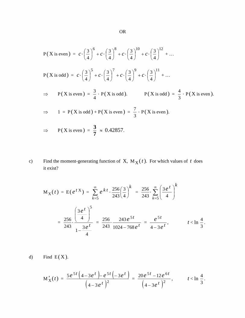
OR

P ( X is even ) = 121086

43

43

43

43

+

+

+

⋅⋅⋅⋅ cccc + …

P ( X is odd ) = 11975

43

43

43

43

+

+

+

⋅⋅⋅⋅ cccc + …

⇒ P ( X is even ) = 43 ⋅ P ( X is odd ). P ( X is odd ) =

34 ⋅ P ( X is even ).

⇒ 1 = P ( X is odd ) + P ( X is even ) = 37 ⋅ P ( X is even ).

⇒ P ( X is even ) = 73 ≈ 0.42857.

c) Find the moment-generating function of X, M X ( t ). For which values of t does it exist?

M X ( t ) = E ( e t X ) = ∑∞

=

⋅

5

43

243256

k

ktke = ∑

∞

=

⋅

5

4 3

243256

k

kte

=

4 31

4 3

243256

5

t

t

e

e

−

⋅ = tt

ee

7681024 243

243256 5

−⋅ = t

t

ee

34

5

−, t < ln

34 .

d) Find E ( X ).

M 'X ( t ) = ( ) ( )( )2

5 5

34

334 5t

tttt

eeeee

−

−−− = ( )2

6 5

34

1220t

tt

eee

−

− , t < ln 34 .

E ( X ) = M 'X ( 0 ) = 8.

OR

E ( X ) = ∑ ⋅x

xpx

all)( =

8765

43

2432568

43

2432567

43

2432566

43

2432565

+

+

+

⋅⋅⋅⋅⋅⋅⋅⋅ + …

43

E ( X ) = 876

43

2432567

43

2432566

43

2432565

+

+

⋅⋅⋅⋅⋅⋅ + …

⇒ 41

E ( X ) = 87655

43

243256

43

243256

43

243256

43

243256

43

2432564

+

+

+

+

⋅⋅⋅⋅⋅⋅ + …

= 1 + ∑∞

=⋅

5

43

243256

k

k = 1 + 1 = 2.

⇒ E ( X ) = 8.

OR

E ( X ) = ∑ ⋅x

xpx

all)( = ∑

∞

=

⋅⋅

5

43

243256

k

kk = ∑

∞

=

−

⋅⋅⋅⋅

5

1

43

41 3

243256

k

kk

=

−

−−−

⋅⋅⋅⋅⋅⋅⋅⋅⋅⋅ ∑

∞

=

− 32

1

1

43

414

43

413

43

412

411

43

41

81256

k

kk

= ( )

−−−−⋅

6427

6427

166

41YE

81256

= = ( )

−⋅

6494YE

81256

,

where Y has a Geometric distribution with probability of “success” p = 41 .

⇒ E ( X ) = ( )

−⋅

6494YE

81256

=

−⋅

64944

81256 =

64162

81256 ⋅ = 8.

OR

p ( k ) = k

c

43

⋅ , k = 5, 6, 7, 8, … , c =

5

4

3

4 .

⇒ p ( k ) = 5

43

41 −

⋅

k, k = 5, 6, 7, 8, … .

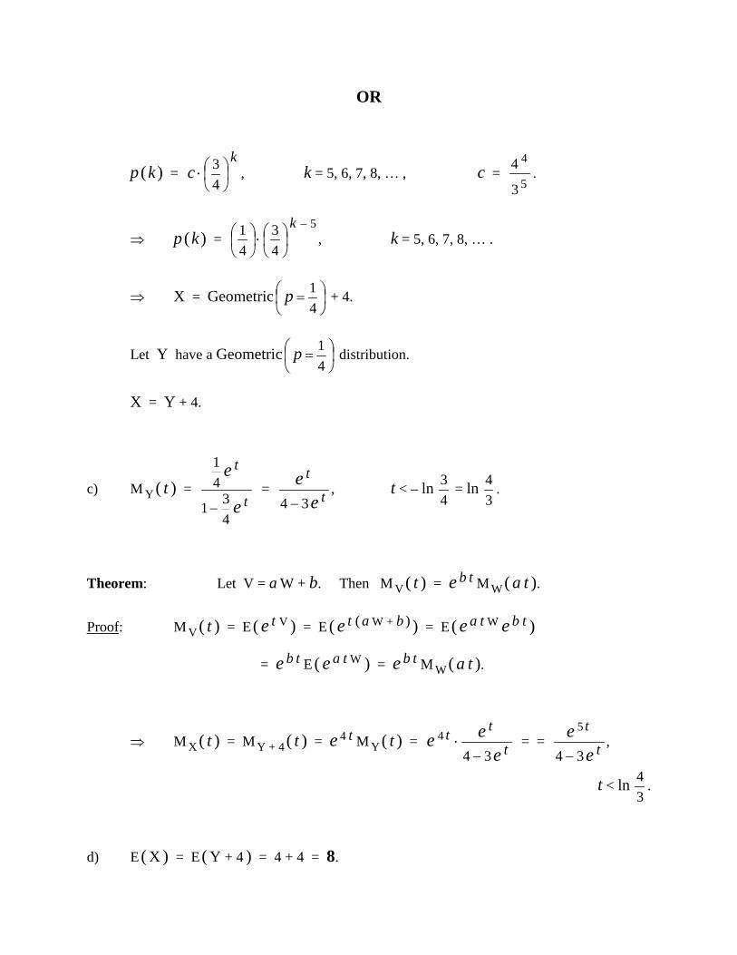
⇒ X = Geometric

=

41p + 4.

Let Y have a Geometric

=

41p distribution.

X = Y + 4.

c) M Y ( t ) = t

t

e

e

431

41

− = t

t

ee

34 −, t < – ln

43 = ln

34 .

Theorem: Let V = a W + b. Then M V ( t ) = e b t M W ( a t ). Proof: M V ( t ) = E ( e t V ) = E ( e t ( a W + b ) ) = E ( e a t W e b t )

= e b t E ( e a t W ) = e b t M W ( a t ).

⇒ M X ( t ) = M Y + 4 ( t ) = e 4 t M Y ( t ) = ttte

ee

34 4

−⋅ = = t

t

ee

34

5

−,

t < ln 34 .

d) E ( X ) = E ( Y + 4 ) = 4 + 4 = 8.

2. Suppose a discrete random variable X has the following probability distribution:

P( X = k ) = ( )!

2lnk

k, k = 1, 2, 3, … .

a) Verify that this is a valid probability distribution.

• p ( x ) ≥ 0 ∀ x

• ( )∑x

xp all

= 1

( )∑∞

=1 ! 2ln

k

k

k = ( )∑

∞

=0 ! 2ln

k

k

k – 1 = e ln 2 – 1 = 2 – 1 = 1.

b) Find µ X = E( X ) by finding the sum of the infinite series.

E ( X ) = ∑ ⋅x

xpx

all)( = ( )∑

∞

=⋅

1 !

2lnk

k

kk = ( )

( )∑∞

−=1 !

12ln

k

k

k

= ( ) ( )( )∑

∞

−=

−⋅

1

1

!

12 2 lnln

k

k

k = ( ) ( )∑

∞

=⋅

0 !

2 2 lnln

k

k

k = 2 ln 2.

c) Find the moment-generating function of X, M X ( t ).

M X ( t ) = ∑ ⋅x

xt

xp eall

)( = ( )∑∞

=⋅

1 !

2lnk

kktk

e = ∑∞

=1 !

2ln

k

kt

k

e

= 1 2ln

−tee = 1 2

−

te .

d) Use M X ( t ) to find µ X = E( X ).

( ) tetet 2 2 M ln

'

X ⋅⋅= , E ( X ) = ( ) 0M ' X = 2 ln 2.

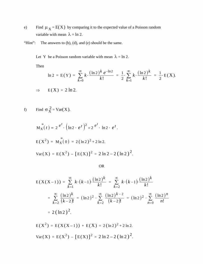
e) Find µ X = E( X ) by comparing it to the expected value of a Poisson random

variable with mean λ = ln 2. “Hint”: The answers to (b), (d), and (e) should be the same. Let Y be a Poisson random variable with mean λ = ln 2. Then

ln 2 = E ( Y ) = ( )∑∞

=

−⋅

0

2

!

ln 2 ln

k

k

kk e = ( )∑

∞

=⋅⋅

1 !

221 ln

k

k

kk = ⋅

21 E ( X ).

⇒ E ( X ) = 2 ln 2. f) Find σ X

2 = Var( X ).

( ) ( ) tt eett eet

2 2 2 2 M lnln

2X

'' ⋅⋅⋅⋅ += .

E ( X 2

) = ( ) 0 M '' X = 2 ( ln 2 )

2 + 2 ln 2.

Var ( X ) = E ( X 2

) – [ E ( X ) ] 2 = 2 ln 2 – 2 ( ln 2 )

2.

OR

E ( X ( X – 1 ) ) = ( ) ( )∑∞

−=

⋅⋅1 !

21 lnk

k

kkk = ( ) ( )∑

∞−

=⋅⋅

2 !

21 lnk

k

kkk

= ( )( )∑

∞

−=2 !

22ln

k

k

k = ( ) ( )

( )∑∞

−=

−⋅

2

22

!

2

2 2 lnlnk

k

k = ( ) ( )∑

∞

=⋅

0

2!

2 2 lnln

n

n

n

= 2 ( ln 2 ) 2.

E ( X 2

) = E ( X ( X – 1 ) ) + E ( X ) = 2 ( ln 2 ) 2 + 2 ln 2.

Var ( X ) = E ( X 2

) – [ E ( X ) ] 2 = 2 ln 2 – 2 ( ln 2 )

2.

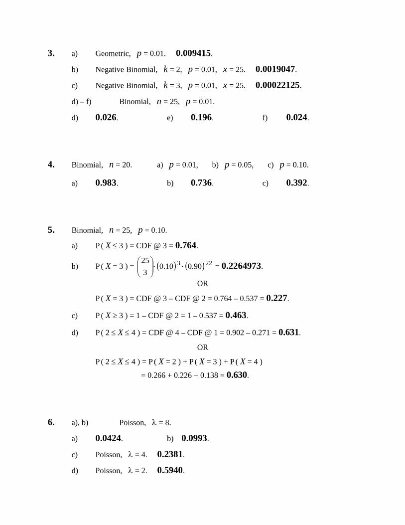
3. a) Geometric, p = 0.01. 0.009415.

b) Negative Binomial, k = 2, p = 0.01, x = 25. 0.0019047.

c) Negative Binomial, k = 3, p = 0.01, x = 25. 0.00022125.

d) – f) Binomial, n = 25, p = 0.01.

d) 0.026. e) 0.196. f) 0.024. 4. Binomial, n = 20. a) p = 0.01, b) p = 0.05, c) p = 0.10.

a) 0.983. b) 0.736. c) 0.392. 5. Binomial, n = 25, p = 0.10. a) P ( X ≤ 3 ) = CDF @ 3 = 0.764.

b) P ( X = 3 ) = ( ) ( )223 90.010.0325 ⋅⋅

= 0.2264973.

OR

P ( X = 3 ) = CDF @ 3 – CDF @ 2 = 0.764 – 0.537 = 0.227. c) P ( X ≥ 3 ) = 1 – CDF @ 2 = 1 – 0.537 = 0.463. d) P ( 2 ≤ X ≤ 4 ) = CDF @ 4 – CDF @ 1 = 0.902 – 0.271 = 0.631.

OR

P ( 2 ≤ X ≤ 4 ) = P ( X = 2 ) + P ( X = 3 ) + P ( X = 4 )

= 0.266 + 0.226 + 0.138 = 0.630. 6. a), b) Poisson, λ = 8.

a) 0.0424. b) 0.0993.

c) Poisson, λ = 4. 0.2381.

d) Poisson, λ = 2. 0.5940.

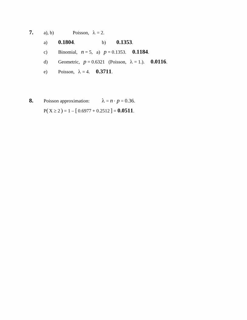
7. a), b) Poisson, λ = 2.

a) 0.1804. b) 0.1353.

c) Binomial, n = 5, a) p = 0.1353. 0.1184.

d) Geometric, p = 0.6321 (Poisson, λ = 1.). 0.0116.

e) Poisson, λ = 4. 0.3711. 8. Poisson approximation: λ = n ⋅ p = 0.36.

P( X ≥ 2 ) = 1 – [ 0.6977 + 0.2512 ] = 0.0511.

9 – 11. Alex sells “Exciting World of Statistics” videos over the phone to earn some extra cash during the economic crisis. Only 10% of all calls result in a sale. Assume that the outcome of each call is independent of the others.

9. a) What is the probability that Alex makes his first sale on the fifth call?

No sale No sale No sale No sale Sale (0.90) • (0.90) • (0.90) • (0.90) • (0.10) = 0.06561. Geometric distribution, p = 0.10. b) What is the probability that Alex makes his first sale on an odd-numbered call?

P(odd) = P(1) + P(3) + P(5) + … = +++ ⋅⋅⋅ 420 90.00.10 90.00.10 90.010.0 …

= 1910

=−

=∞

=∞

⋅⋅⋅ ∑∑== 81.01

110.081.010.090.010.000

2

nn

kk ≈ 0.5263.

OR P(odd) = +++ ⋅⋅⋅ 420 90.00.10 90.00.10 90.010.0 …

P(even) = +++ ⋅⋅⋅ 531 90.00.10 90.00.10 90.010.0 … ⇒ P(even) = 0.90 ⋅ P(odd).

⇒ 1 = P(odd) + P(even) = 1.9 ⋅ P(odd). P(odd) = 1910 ≈ 0.5263.

c) What is the probability that it takes Alex at least 10 calls to make his first sale? For Geometric distribution, X = number of independent attempts needed to get the first “success”. P ( X > a ) = P ( the first a attempts are “failures” ) = ( 1 – p )

a, a = 0, 1, 2, 3, … . P ( X ≥ 10 ) = P ( X > 9 ) = 0.90

9 ≈ 0.38742. d) What is the probability that it takes Alex at most 6 calls to make his first sale? P ( X ≤ 6 ) = 1 – P ( X > 6 ) = 1 – 0.90

6 = 0.468559. 10. e) What is the probability that Alex makes his second sale on the ninth call? [ 8 calls: 1 S & 7 F’s ] S

( ) ( )[ ] 90.010.018 71

⋅⋅C ⋅ 0.10 ≈ 0.038264.

OR Let Y = the number of (independent) calls needed to make 2 sales.

⇒ Negative Binomial distribution, k = 2, p = 0.10. kyk ppkCyyY −−−−== ⋅⋅ )1( 11)P(

P(Y = 13) = ( ) ( )72 90.010.018 ⋅⋅C ≈ 0.038264.

f) What is the probability that Alex makes his second sale on an odd-numbered call? Hint: Consider [ Answer ] – 0.9

2 × [ Answer ]. On one side, you will have 0.19 × [ Answer ]. On the other side, you will have a geometric series. Let Y = the number of (independent) calls needed to make 2 sales.

⇒ Negative Binomial distribution, k = 2, p = 0.10. kykkyk ppyppCyyY −− −−=−−== ⋅⋅⋅⋅ )1( )1()1( 11)P( , y = 2, 3, 4, 5,

… . [ Answer ] = f ( 3 ) + f ( 5 ) + f ( 7 ) + f ( 9 ) + …

= ++++ ⋅⋅⋅⋅⋅⋅⋅⋅ 72523212 90.0.1008 90.0.1006 90.0.1004 90.010.02 …

0.81 × [ Answer ] = 0.9 2 × [ Answer ]

= +++ ⋅⋅⋅⋅⋅⋅ 725232 90.0.1006 90.0.1004 90.010.02 …

0.19 × [ Answer ] = [ Answer ] − 0.81 × [ Answer ]

= ++++ ⋅⋅⋅⋅⋅⋅⋅⋅ 72523212 90.0.1002 90.0.1002 90.0.1002 90.010.02

…

= basetermfirst

−1 =

2

12

90.01

90.010.02

−

⋅⋅ = 19.0018.0 .

[ Answer ] = 2 19.0

018.0 = 0361.0018.0 =

361180 ≈ 0.498615.

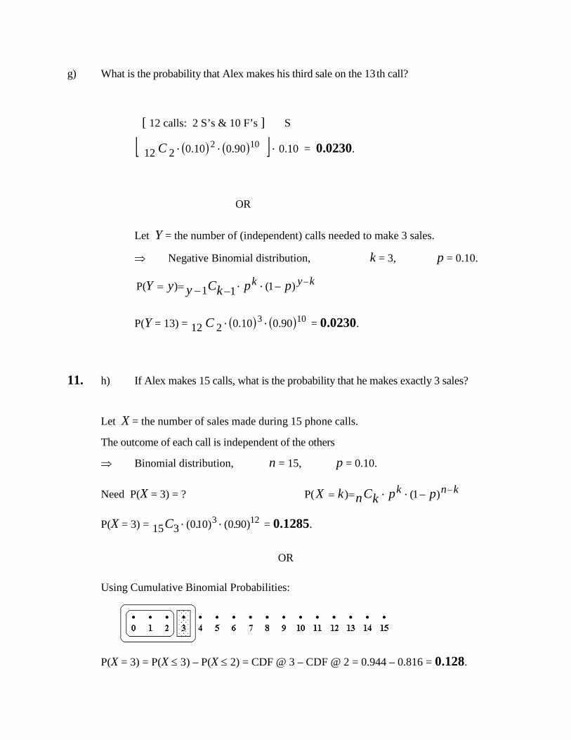
g) What is the probability that Alex makes his third sale on the 13 th call? [ 12 calls: 2 S’s & 10 F’s ] S

( ) ( )[ ] 90.010.0212 102

⋅⋅C ⋅ 0.10 = 0.0230. OR

Let Y = the number of (independent) calls needed to make 3 sales.

⇒ Negative Binomial distribution, k = 3, p = 0.10. kyk ppkCyyY −−−−== ⋅⋅ )1( 11)P(

P(Y = 13) = ( ) ( )103 90.010.0212 ⋅⋅C = 0.0230. 11. h) If Alex makes 15 calls, what is the probability that he makes exactly 3 sales? Let X = the number of sales made during 15 phone calls.

The outcome of each call is independent of the others

⇒ Binomial distribution, n = 15, p = 0.10. Need P(X = 3) = ? knk ppkCnkX −−== ⋅⋅ )1( )P(

P(X = 3) = 123 )900()100(315 ..C ⋅⋅ = 0.1285.

OR Using Cumulative Binomial Probabilities:

P(X = 3) = P(X ≤ 3) – P(X ≤ 2) = CDF @ 3 – CDF @ 2 = 0.944 – 0.816 = 0.128.

i) If Alex makes 15 calls, what is the probability that he makes at least 2 sales? Need P(X ≥ 2) = ? P(X ≥ 2) = 1 − P(X = 0) − P(X = 1)

= 141150 )900()100(115 )900()100(015 1 .... CC ⋅⋅⋅⋅ −−

= 1 − 0.2059 − 0.3432 = 0.4509.

OR Using Cumulative Binomial Probabilities:

P(X ≥ 2) = 1 – P(X ≤ 1) = 1 – CDF @ 1 = 1 – 0.549 = 0.451. j) If Alex makes 15 calls, what is the probability that he makes at most 2 sales? P(X ≤ 2) = 132141150 )900()100(215 )900()100(115 )900()100(015 ...... CCC ⋅⋅⋅⋅⋅⋅ ++

= 0.2059 + 0.3432 + 0.2669 = 0.8160.

OR P(X ≤ 2) = CDF @ 2 = 0.816.

10.

a) Let X have a Poisson distribution with variance of 3. Find P ( X = 2 ). Poisson distribution: Var ( X ) = λ ⇒ λ = 3

Thus, P ( X = 2 ) = ! 2

λ λ2 −e = ! 2

3 32 −e = 0.22404.

OR

Table III P ( X = 2 ) = P ( X ≤ 2 ) – P ( X ≤ 1 ) = 0.423 – 0.199 = 0.224. b) If X has a Poisson distribution such that 3 P ( X = 1 ) = P ( X = 2 ), find P ( X = 4 ).

!! 2

λ 1 λ 3

λ2λ1 −−=⋅ ee ⇒ 6 λ = λ

2

⇒ λ = 6 since λ > 0.

Thus, P ( X = 4 ) = ! 4

λ λ4 −e = ! 4

6 64 −e = 0.13385.

OR

Table III P ( X = 4 ) = P ( X ≤ 4 ) – P ( X ≤ 3 ) = 0.285 – 0.151 = 0.134.

11. Suppose the number of air bubbles in window glass has a Poisson distribution, with an average of 0.3 air bubbles per square foot. In a 4 ' by 3 ' window, find the probability that there are … 4 ' by 3 ' = 12 square feet. λ = 0.3 × 12 = 3.6. a) … exactly 5 air bubbles.

P ( X = 5 ) = !5

6.3 6.35

e −⋅ = 0.13768.

OR

Table III P ( X = 5 ) = P ( X ≤ 5 ) – P ( X ≤ 4 ) = 0.844 – 0.706 = 0.138. b) … at least 5 air bubbles. Table III P ( X ≥ 5 ) = 1 – P ( X ≤ 4 ) = 1 – 0.706 = 0.294.

OR

P ( X = 5 ) = 1 – P ( X = 0 ) – P ( X = 1 ) – P ( X = 2 ) – P ( X = 3 ) – P ( X = 4 )

= !

!

!

!

!

4 6.3

3 6.3

2 6.3

1 6.3

0 6.31

6.346.336.326.316.30 −−−−− ⋅⋅⋅⋅⋅−−−−−

eeeee

= 1 – 0.02732 – 0.09837 – 0.17706 – 0.21247 – 0.19122 = 1 – 0.70644 = 0.29356.

From the textbook: 2.4-10 2.4-12 2.4.14 (a) X is b(8, 0.90), Binomial distribution with n = 8 and p = 0.90;

(b) (i) P(X = 8) = ( ) ( )08 1.0 9.0 88

= 0.43046721;

(ii) P(X ≤ 6) = 1 – P(X = 7) – P(X = 8)

= ( ) ( ) ( ) ( )0817 1.0 9.0 88

1.0 9.0 78

1

−

− = 0.18689527;

(iii) P(X ≥ 6) = P(X = 6) + P(X = 7) + P(X = 8)

= ( ) ( ) ( ) ( ) ( ) ( )081726 1.0 9.0 88

1.0 9.0 78

1.0 9.0 68

+

+

= 0.96190821.

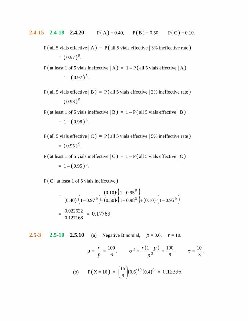
2.4-15 2.4-18 2.4.20 P ( A ) = 0.40, P ( B ) = 0.50, P ( C ) = 0.10.

P ( all 5 vials effective | A ) = P ( all 5 vials effective | 3% ineffective rate )

= ( 0.97 ) 5.

P ( at least 1 of 5 vials ineffective | A ) = 1 – P ( all 5 vials effective | A )

= 1 – ( 0.97 ) 5.

P ( all 5 vials effective | B ) = P ( all 5 vials effective | 2% ineffective rate )

= ( 0.98 ) 5.

P ( at least 1 of 5 vials ineffective | B ) = 1 – P ( all 5 vials effective | B )

= 1 – ( 0.98 ) 5.

P ( all 5 vials effective | C ) = P ( all 5 vials effective | 5% ineffective rate )

= ( 0.95 ) 5.

P ( at least 1 of 5 vials ineffective | C ) = 1 – P ( all 5 vials effective | C )

= 1 – ( 0.95 ) 5.

P ( C | at least 1 of 5 vials ineffective )

= ( ) ( )( ) ( ) ( ) ( ) ( ) ( )

555

5

95.01 10.098.01 50.097.01 40.095.01 10.0

−+−+−

−

⋅⋅⋅⋅

= 127168.0022622.0 = 0.17789.

2.5-3 2.5-10 2.5.10 (a) Negative Binomial, p = 0.6, r = 10. µ =

pr =

6100 , σ

2 = ( )2

1 p

pr − = 9

100 , σ = 3

10 .

(b) P ( X = 16 ) = ( ) ( )610 4.0 6.0 9

15

= 0.12396.

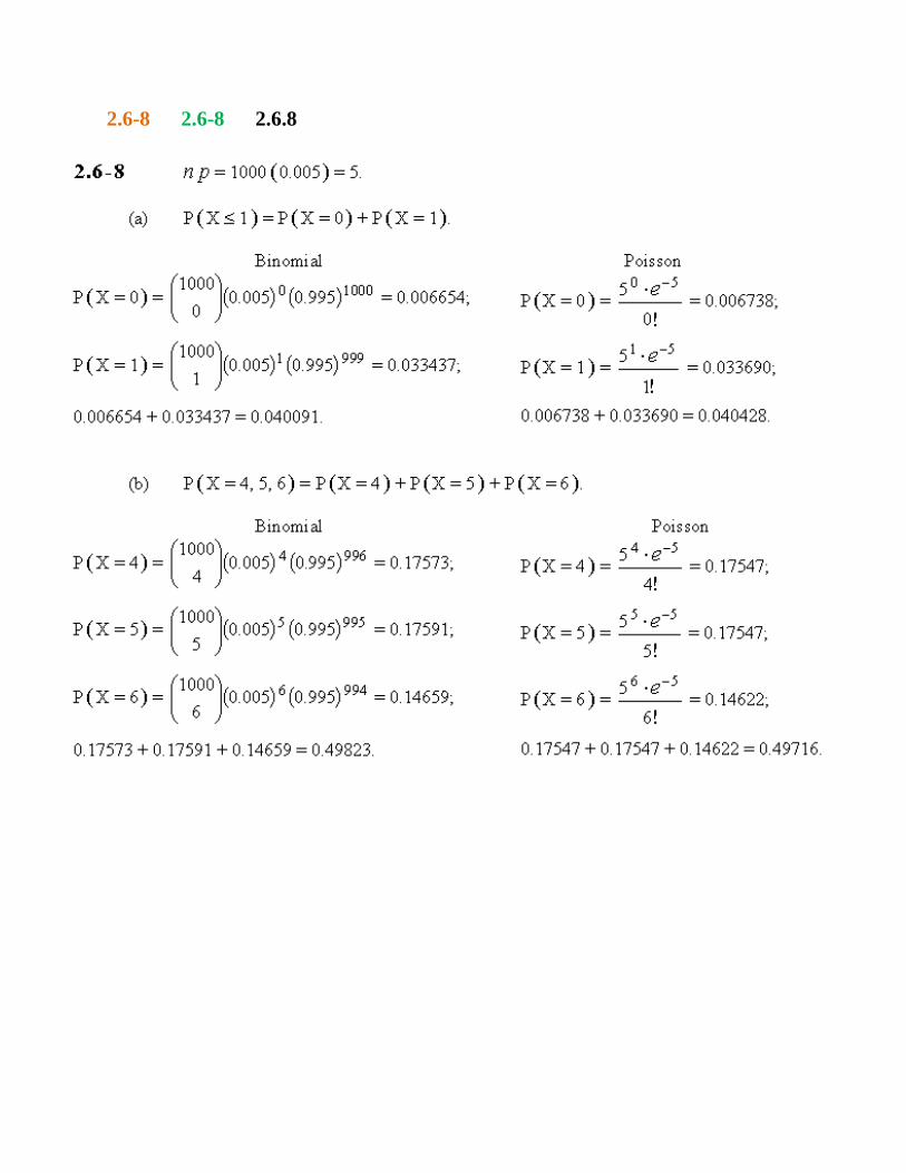
2.6-8 2.6-8 2.6.8