1

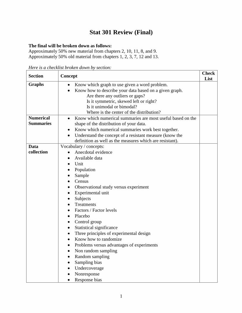
Stat 301 Review (Final)

The final will be broken down as follows:

Approximately 50% new material from chapters 2, 10, 11, 8, and 9.

Approximately 50% old material from chapters 1, 2, 3, 7, 12 and 13.

Here is a checklist broken down by section:

Section Concept Check

List

Graphs Know which graph to use given a word problem.

Know how to describe your data based on a given graph.

Are there any outliers or gaps?

Is it symmetric, skewed left or right?

Is it unimodal or bimodal?

Where is the center of the distribution?

Numerical

Summaries Know which numerical summaries are most useful based on the

shape of the distribution of your data.

Know which numerical summaries work best together.

Understand the concept of a resistant measure (know the

definition as well as the measures which are resistant).

Data

collection

Vocabulary / concepts:

Anecdotal evidence

Available data

Unit

Population

Sample

Census

Observational study versus experiment

Experimental unit

Subjects

Treatments

Factors / Factor levels

Placebo

Control group

Statistical significance

Three principles of experimental design

Know how to randomize

Problems versus advantages of experiments

Non random sampling

Random sampling

Sampling bias

Undercoverage

Nonresponse

Response bias

2

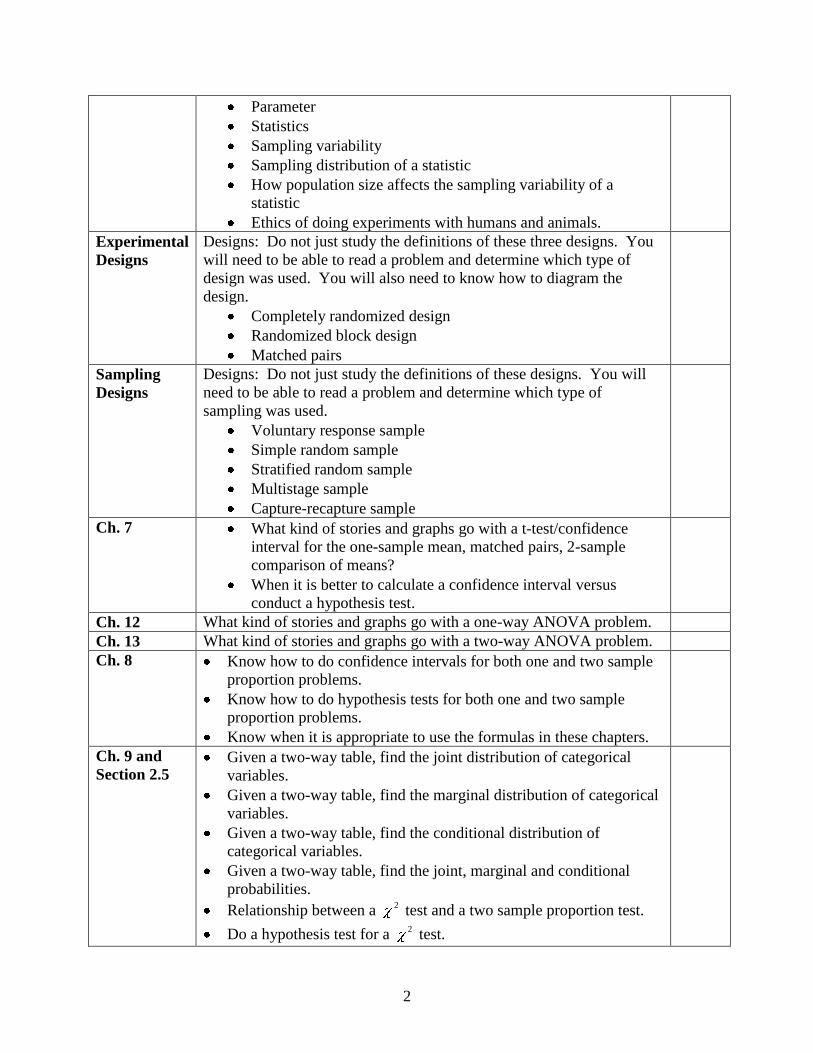
Parameter

Statistics

Sampling variability

Sampling distribution of a statistic

How population size affects the sampling variability of a

statistic

Ethics of doing experiments with humans and animals.

Experimental

Designs

Designs: Do not just study the definitions of these three designs. You

will need to be able to read a problem and determine which type of

design was used. You will also need to know how to diagram the

design.

Completely randomized design

Randomized block design

Matched pairs

Sampling

Designs

Designs: Do not just study the definitions of these designs. You will

need to be able to read a problem and determine which type of

sampling was used.

Voluntary response sample

Simple random sample

Stratified random sample

Multistage sample

Capture-recapture sample

Ch. 7 What kind of stories and graphs go with a t-test/confidence

interval for the one-sample mean, matched pairs, 2-sample

comparison of means?

When it is better to calculate a confidence interval versus

conduct a hypothesis test.

Ch. 12 What kind of stories and graphs go with a one-way ANOVA problem.

Ch. 13 What kind of stories and graphs go with a two-way ANOVA problem.

Ch. 8 Know how to do confidence intervals for both one and two sample

proportion problems.

Know how to do hypothesis tests for both one and two sample

proportion problems.

Know when it is appropriate to use the formulas in these chapters.

Ch. 9 and

Section 2.5 Given a two-way table, find the joint distribution of categorical

variables.

Given a two-way table, find the marginal distribution of categorical

variables.

Given a two-way table, find the conditional distribution of

categorical variables.

Given a two-way table, find the joint, marginal and conditional

probabilities.

Relationship between a 2 test and a two sample proportion test.

Do a hypothesis test for a 2 test.

3

Know when it is appropriate to use a 2 test.

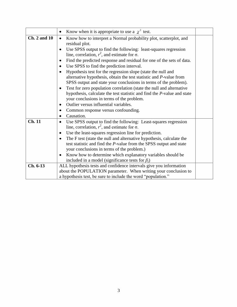
Ch. 2 and 10 Know how to interpret a Normal probability plot, scatterplot, and

residual plot.

Use SPSS output to find the following: least-squares regression

line, correlation, r2, and estimate for σ.

Find the predicted response and residual for one of the sets of data.

Use SPSS to find the prediction interval.

Hypothesis test for the regression slope (state the null and

alternative hypothesis, obtain the test statistic and P-value from

SPSS output and state your conclusions in terms of the problem).

Test for zero population correlation (state the null and alternative

hypothesis, calculate the test statistic and find the P-value and state

your conclusions in terms of the problem.

Outlier versus influential variables.

Common response versus confounding.

Causation.

Ch. 11 Use SPSS output to find the following: Least-squares regression

line, correlation, r2, and estimate for σ.

Use the least-squares regression line for prediction.

The F test (state the null and alternative hypothesis, calculate the

test statistic and find the P-value from the SPSS output and state

your conclusions in terms of the problem.)

Know how to determine which explanatory variables should be

included in a model (significance tests for βj)

Ch. 6-13 ALL hypothesis tests and confidence intervals give you information

about the POPULATION parameter. When writing your conclusion to

a hypothesis test, be sure to include the word “population.”

4

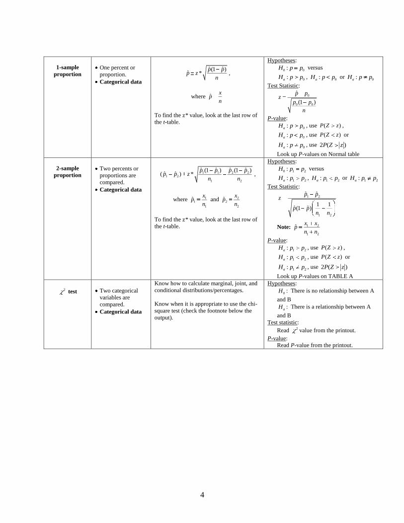
1-sample

proportion

One percent or

proportion.

Categorical data

ˆ ˆ(1 )ˆ *

p pp z

n,

where ˆx

pn

To find the z* value, look at the last row of

the t-table.

Hypotheses:

0 0:H p p versus

0:aH p p , 0:aH p p or

0:aH p p

Test Statistic:

0

0 0

ˆ

(1 )

p pz

p p

n

P-value:

0:aH p p , use ( )P Z z ,

0:aH p p , use ( )P Z z or

0:aH p p , use 2 ( )P Z z

Look up P-values on Normal table

2-sample

proportion

Two percents or

proportions are

compared.

Categorical data

1 1 2 21 2

1 2

ˆ ˆ ˆ ˆ(1 ) (1 )ˆ ˆ( ) *

p p p pp p z

n n,

where 11

1

ˆx

pn

and 22

2

ˆx

pn

To find the z* value, look at the last row of

the t-table.

Hypotheses:

0 1 2:H p p versus

1 2:aH p p , 1 2:aH p p or

1 2:aH p p

Test Statistic:

1 2

1 2

ˆ ˆ

1 1ˆ ˆ(1 )

p pz

p pn n

Note: 1 2

1 2

ˆx x

pn n

P-value:

1 2:aH p p , use ( )P Z z ,

1 2:aH p p , use ( )P Z z or

1 2:aH p p , use 2 ( )P Z z

Look up P-values on TABLE A

2 test

Two categorical

variables are

compared.

Categorical data

Know how to calculate marginal, joint, and

conditional distributions/percentages.

Know when it is appropriate to use the chi-

square test (check the footnote below the

output).

Hypotheses:

0H : There is no relationship between A

and B

aH : There is a relationship between A

and B

Test statistic:

Read 2 value from the printout.

P-value:

Read P-value from the printout.

5

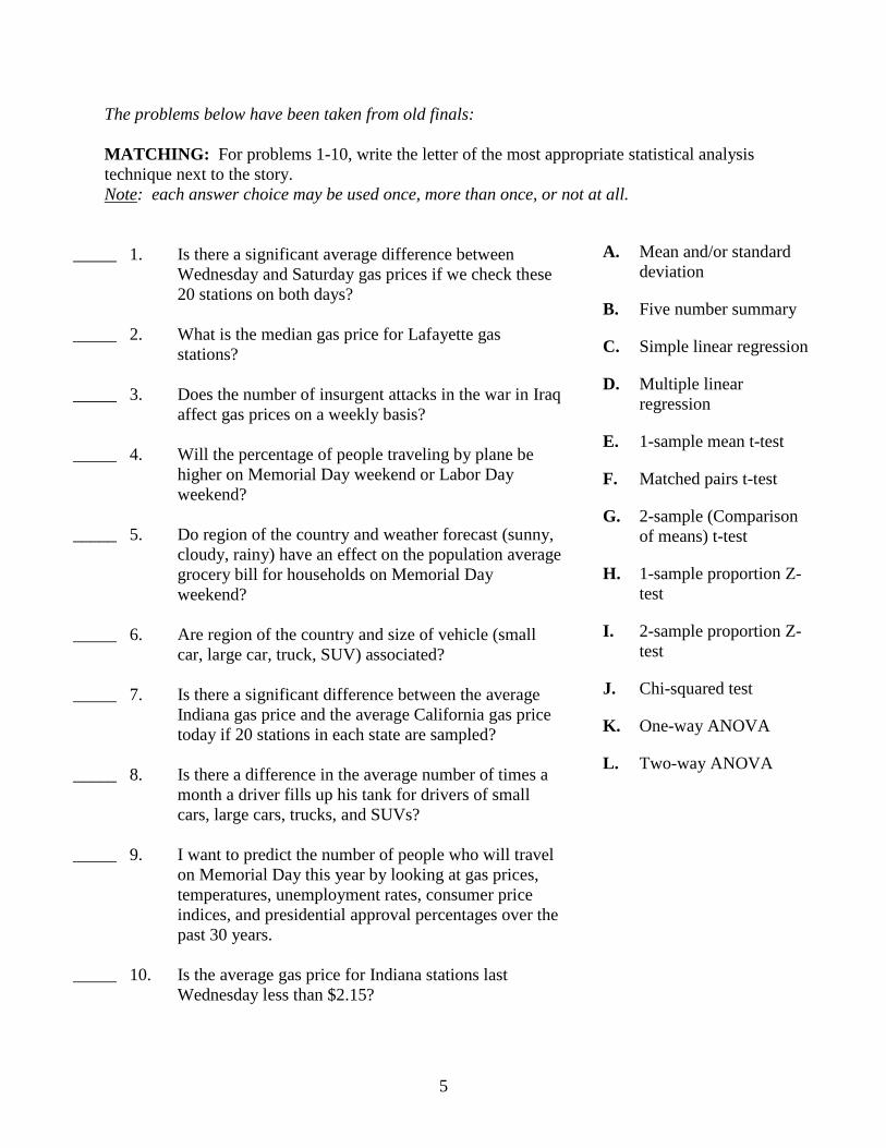
The problems below have been taken from old finals:

MATCHING: For problems 1-10, write the letter of the most appropriate statistical analysis

technique next to the story.

Note: each answer choice may be used once, more than once, or not at all.

_____ 1. Is there a significant average difference between

Wednesday and Saturday gas prices if we check these

20 stations on both days?

_____ 2. What is the median gas price for Lafayette gas

stations?

_____ 3. Does the number of insurgent attacks in the war in Iraq

affect gas prices on a weekly basis?

_____ 4. Will the percentage of people traveling by plane be

higher on Memorial Day weekend or Labor Day

weekend?

_____ 5. Do region of the country and weather forecast (sunny,

cloudy, rainy) have an effect on the population average

grocery bill for households on Memorial Day

weekend?

_____ 6. Are region of the country and size of vehicle (small

car, large car, truck, SUV) associated?

_____ 7. Is there a significant difference between the average

Indiana gas price and the average California gas price

today if 20 stations in each state are sampled?

_____ 8. Is there a difference in the average number of times a

month a driver fills up his tank for drivers of small

cars, large cars, trucks, and SUVs?

_____ 9. I want to predict the number of people who will travel

on Memorial Day this year by looking at gas prices,

temperatures, unemployment rates, consumer price

indices, and presidential approval percentages over the

past 30 years.

_____ 10. Is the average gas price for Indiana stations last

Wednesday less than $2.15?

A. Mean and/or standard

deviation

B. Five number summary

C. Simple linear regression

D. Multiple linear

regression

E. 1-sample mean t-test

F. Matched pairs t-test

G. 2-sample (Comparison

of means) t-test

H. 1-sample proportion Z-

test

I. 2-sample proportion Z-

test

J. Chi-squared test

K. One-way ANOVA

L. Two-way ANOVA

6

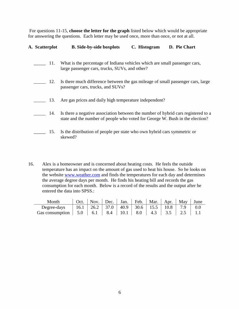
For questions 11-15, choose the letter for the graph listed below which would be appropriate

for answering the questions. Each letter may be used once, more than once, or not at all.

A. Scatterplot B. Side-by-side boxplots C. Histogram D. Pie Chart

_____ 11. What is the percentage of Indiana vehicles which are small passenger cars,

large passenger cars, trucks, SUVs, and other?

_____ 12. Is there much difference between the gas mileage of small passenger cars, large

passenger cars, trucks, and SUVs?

_____ 13. Are gas prices and daily high temperature independent?

_____ 14. Is there a negative association between the number of hybrid cars registered to a

state and the number of people who voted for George W. Bush in the election?

_____ 15. Is the distribution of people per state who own hybrid cars symmetric or

skewed?

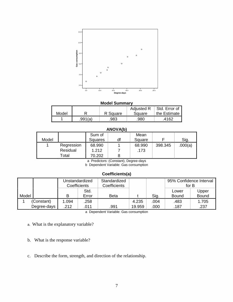
16. Alex is a homeowner and is concerned about heating costs. He feels the outside

temperature has an impact on the amount of gas used to heat his house. So he looks on

the website www.weather.com and finds the temperatures for each day and determines

the average degree days per month. He finds his heating bill and records the gas

consumption for each month. Below is a record of the results and the output after he

entered the data into SPSS.:

Month Oct. Nov. Dec. Jan. Feb. Mar. Apr. May June

Degree-days

Gas consumption

16.1

5.0

26.2

6.1

37.0

8.4

40.9

10.1

30.6

8.0

15.5

4.3

10.8

3.5

7.9

2.5

0.0

1.1

7

0.0 10.0 20.0 30.0 40.0 50.0

Degree-days

0.0

3.0

6.0

9.0

12.0

15.0

Gas c

on

su

mp

tio

n

Model Summary

Model R R Square Adjusted R

Square Std. Error of the Estimate

1 .991(a) .983 .980 .4162

ANOVA(b)

Model Sum of Squares df

Mean Square F Sig.

1 Regression 68.990 1 68.990 398.345 .000(a)

Residual 1.212 7 .173

Total 70.202 8 a Predictors: (Constant), Degree-days

b Dependent Variable: Gas consumption

Coefficients(a)

a Dependent Variable: Gas consumption

a. What is the explanatory variable?

b. What is the response variable?

c. Describe the form, strength, and direction of the relationship.

Model

Unstandardized Coefficients

Standardized Coefficients

t Sig.

95% Confidence Interval for B

B Std. Error Beta

Lower Bound

Upper Bound

1 (Constant) 1.094 .258 4.235 .004 .483 1.705

Degree-days .212 .011 .991 19.959 .000 .187 .237

8

d. What is the equation of the least squares regression line for the heating season?

e. What is the predicted gas consumption when degree-days is 30.6?

f. Find the residual value when degree days is 30.6.

g. How much of the variation in gas consumption is explained by the least-squares regression?

h. Do a test to determine if there is a linear relationship between degree-days and gas

consumption. State your hypotheses, test statistic, P-value, and your conclusion in terms of

the story.

9

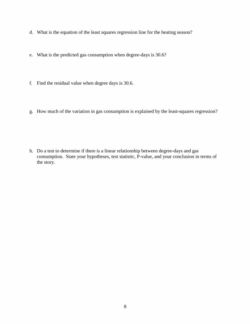
17. As an avid supporter of Purdue’s football team, Pete wants to do a little analysis. He took a

random sample of 15 games from the last three seasons. He thinks that the number of fans at

each game may affect the number of points Purdue scores. The output from his analysis is

below:

Attendance at Game

120000110000100000900008000070000600005000040000

Poin

ts P

urd

ue S

co

red

70

60

50

40

30

20

10

0

Model Summary

.611a .373 .325 11.028

Model

1

R R Square

Adjusted

R Square

Std. Error of

the Estimate

Predictors: (Constant), Attendance at Gamea.

ANOVAb

942.048 1 942.048 7.747 .016a

1580.886 13 121.607

2522.933 14

Regression

Residual

Total

Model

1

Sum of Squares df Mean Square F Sig.

Predictors: (Constant), Attendance at Gamea.

Dependent Variable: Points Purdue Scoredb.

10

a. What is the explanatory variable?

b. What is the response variable?

c. Describe the form, strength, and direction of the relationship.

d. What is the equation of the least squares regression line for the number of points scored?

e. What is the predicted number of points scored when the attendance is 56,400?

f. When the attendance was 56,400, Purdue scored 31 points. What is its residual?

g. How much of the variation in number of points scored by Purdue is explained by the

least-squares regression?

h. Do a test to determine if there is a negative linear relationship between attendance at

games and number of points scored by Purdue. State your hypotheses, test statistic, P-

value, and your conclusion in terms of the story.

11

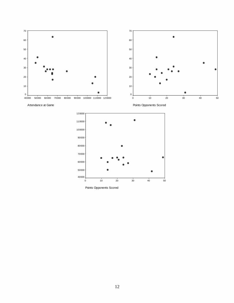
18. After thinking some more, Pete thought there could be other variables that might affect the

number of points Purdue scored. One variable of interest is the number of points the

opponent scores. He added this variable to his analysis and did a multiple regression.

a. Using the output on the next four pages, what is the best equation of a line for predicting

the number of points Purdue scored in a game? (use α = 0.1)

b. Give 4 reasons for why you made that choice.

Correlations

1 -.611* .075

. .016 .790

15 15 15

-.611* 1 -.157

.016 . .576

15 15 15

.075 -.157 1

.790 .576 .

15 15 15

Pearson Correlation

Sig. (2-tailed)

N

Pearson Correlation

Sig. (2-tailed)

N

Pearson Correlation

Sig. (2-tailed)

N

Points Purdue Scored

Attendance at Game

Points Opponents Scored

Points Purdue

Scored

Attendance

at Game

Points Opponents

Scored

Correlation is significant at the 0.05 level (2-tailed).*.

12

Attendance at Game

120000110000100000900008000070000600005000040000

Poin

ts P

urd

ue S

co

red

70

60

50

40

30

20

10

0

Points Opponents Scored

50403020100

Poin

ts P

urd

ue S

co

red

70

60

50

40

30

20

10

0

Points Opponents Scored

50403020100

Atte

nd

an

ce

at

Gam

e

120000

110000

100000

90000

80000

70000

60000

50000

40000

13

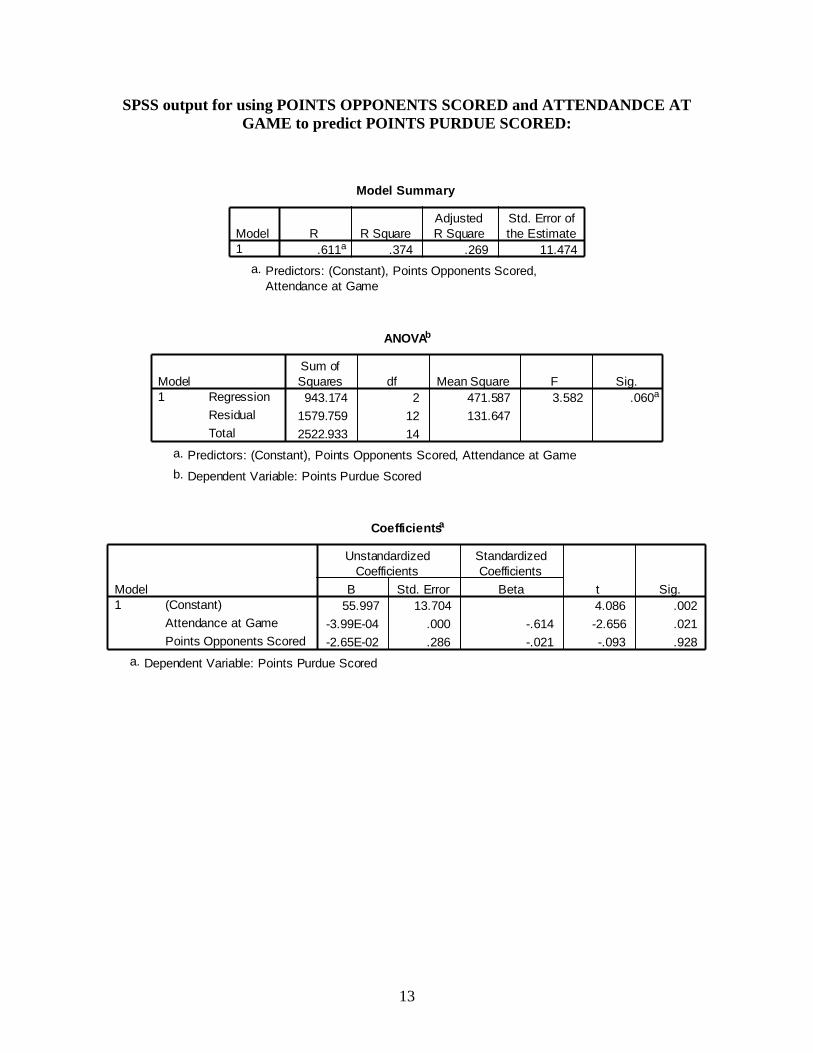
SPSS output for using POINTS OPPONENTS SCORED and ATTENDANDCE AT

GAME to predict POINTS PURDUE SCORED:

Model Summary

.611a .374 .269 11.474

Model

1

R R Square

Adjusted

R Square

Std. Error of

the Estimate

Predictors: (Constant), Points Opponents Scored,

Attendance at Game

a.

ANOVAb

943.174 2 471.587 3.582 .060a

1579.759 12 131.647

2522.933 14

Regression

Residual

Total

Model

1

Sum of

Squares df Mean Square F Sig.

Predictors: (Constant), Points Opponents Scored, Attendance at Gamea.

Dependent Variable: Points Purdue Scoredb.

Coefficientsa

55.997 13.704 4.086 .002

-3.99E-04 .000 -.614 -2.656 .021

-2.65E-02 .286 -.021 -.093 .928

(Constant)

Attendance at Game

Points Opponents Scored

Model

1

B Std. Error

Unstandardized

Coefficients

Beta

Standardized

Coefficients

t Sig.

Dependent Variable: Points Purdue Scoreda.

14

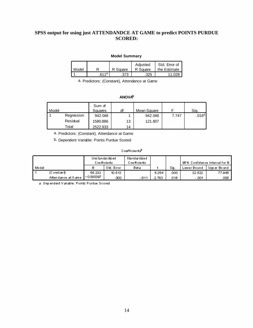
SPSS output for using just ATTENDANDCE AT GAME to predict POINTS PURDUE

SCORED:

Model Summary

.611a .373 .325 11.028

Model

1

R R Square

Adjusted

R Square

Std. Error of

the Estimate

Predictors: (Constant), Attendance at Gamea.

ANOVAb

942.048 1 942.048 7.747 .016a

1580.886 13 121.607

2522.933 14

Regression

Residual

Total

Model

1

Sum of

Squares df Mean Square F Sig.

Predictors: (Constant), Attendance at Gamea.

Dependent Variable: Points Purdue Scoredb.

15

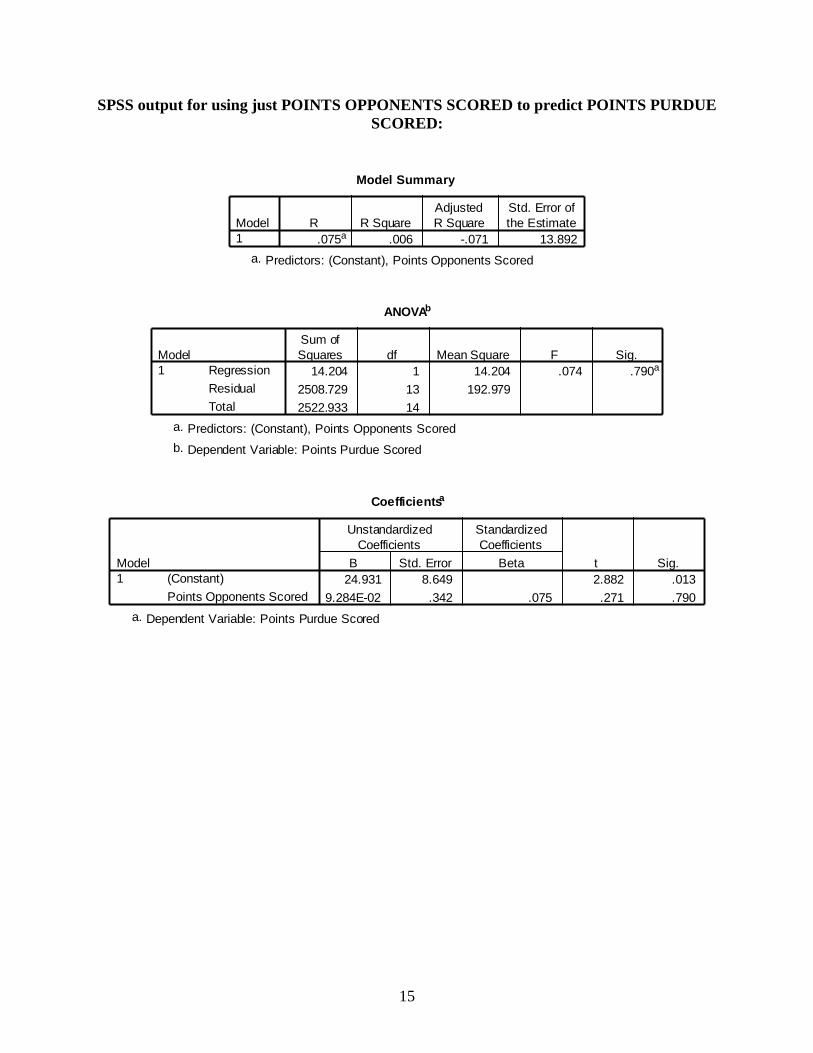
SPSS output for using just POINTS OPPONENTS SCORED to predict POINTS PURDUE

SCORED:

Model Summary

.075a .006 -.071 13.892

Model

1

R R Square

Adjusted

R Square

Std. Error of

the Estimate

Predictors: (Constant), Points Opponents Scoreda.

ANOVAb

14.204 1 14.204 .074 .790a

2508.729 13 192.979

2522.933 14

Regression

Residual

Total

Model

1

Sum of

Squares df Mean Square F Sig.

Predictors: (Constant), Points Opponents Scoreda.

Dependent Variable: Points Purdue Scoredb.

Coefficientsa

24.931 8.649 2.882 .013

9.284E-02 .342 .075 .271 .790

(Constant)

Points Opponents Scored

Model

1

B Std. Error

Unstandardized

Coefficients

Beta

Standardized

Coefficients

t Sig.

Dependent Variable: Points Purdue Scoreda.

16

19. An environmental health professor conducted a study to see whether fast-food workers

wearing gloves actually lowers the chance that customers will come down with food

poisoning. The scientists purchased 371 tortillas from several local fast-food restaurants,

noting whether the workers were wearing gloves or not. 190 of the tortillas came from bare-

hands restaurants; 181 of the tortillas came from glove-wearing restaurants. The scientists

then tested the tortillas purchased for microbe growth. They found that the bare-hands

restaurants’ tortillas gave rise to microbe growth on 18 tortillas, and the glove-wearing

restaurants’ tortillas gave rise to microbe growth only on 8 tortillas. Is the glove-wearing

restaurants’ tortillas’ microbe growth significantly lower than the bare-hands restaurants’

microbe growth at the 5% significance level?

1. State your hypotheses for this test.

2. Calculate your test statistic.

3. Find your P-value.

4. State your conclusion in terms of the story.

17

20. In a 1984 survey of licensed drivers in Wisconsin, 214 of 1200 men said that they did not

drink alcohol. Construct a 95% confidence interval for the proportion of men who said that

they did not drink alcohol. Is your confidence interval calculation reasonable? Why?

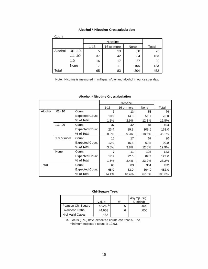
21. On the next page is the SPSS output for a study of alcohol and nicotine consumption among

452 pregnant women. Nicotine consumption is divided into 3 categories, and alcohol

consumption is divided into 4 categories. Answer the questions below based on the output

that follows.

a. What proportion of the non-alcohol consuming women do not smoke during pregnancy?

Is this a joint, marginal or conditional probability?

b. What proportion of women do not smoke and do not consume alcohol during pregnancy?

Is this a joint, marginal or conditional probability?

c. Find the marginal distribution for alcohol consumption during pregnancy.

d. State the null and alternative hypotheses to test whether there is a relationship between

alcohol consumption and smoking during pregnancy.

e. What are the test statistic and P-value used to test the hypotheses in part d?

f. State your conclusions in terms of the original problem.

g. Are your results for the above test valid? Explain your answer.

18

Alcohol * Nicotine Crosstabula tion

Count

5 13 58 76

37 42 84 163

16 17 57 90

7 11 105 123

65 83 304 452

.01-.10

.11-.99

1.0

None

Alcohol

Total

1-15 16 or more None

Nicotine

Total

Note: Nicotine is measured in milligrams/day and alcohol in ounces per day.

Chi-Square Tests

42.252a 6 .000

44.653 6 .000

452

Pearson Chi-Square

Likelihood Ratio

N of Valid Cases

Value df

Asymp. Sig.

(2-s ided)

0 cells (.0%) have expected count less than 5. The

minimum expected count is 10.93.

a.

Alcohol * Nicotine Crosstabulation

5 13 58 76

10.9 14.0 51.1 76.0

1.1% 2.9% 12.8% 16.8%

37 42 84 163

23.4 29.9 109.6 163.0

8.2% 9.3% 18.6% 36.1%

16 17 57 90

12.9 16.5 60.5 90.0

3.5% 3.8% 12.6% 19.9%

7 11 105 123

17.7 22.6 82.7 123.0

1.5% 2.4% 23.2% 27.2%

65 83 304 452

65.0 83.0 304.0 452.0

14.4% 18.4% 67.3% 100.0%

Count

Expected Count

% of Total

Count

Expected Count

% of Total

Count

Expected Count

% of Total

Count

Expected Count

% of Total

Count

Expected Count

% of Total

.01-.10

.11-.99

1.0 or more

None

Alcohol

Total

1-15 16 or more None

Nicotine

Total

19

Multiple Choice: Circle the letter of the correct answer and write its letter in the blank next to

each story.

_____ 22. Does bread lose its vitamins when stored? Twenty small loaves of bread were

randomly assigned to one of four storage times (one, two, three, or four days). After

the bread had been stored for its respective amount of days, its vitamin C content was

measured. This is an example of a

A. simple random sample.

B. completely randomized design.

C. randomized block design.

D. matched pairs design.

E. stratified random sample.

_____ 23. The department of health wanted to know how many people received flu shots this

year. They thought that females were more likely to get a shot, so they randomly

selected 500 males and 500 females in Lafayette and West Lafayette to survey. This

is an example of a

A. simple random sample.

B. completely randomized design.

C. randomized block design.

D. matched pairs design.

E. stratified random sample.

_____24. Which of the following is a potential way to reduce sampling variability?

A. Increase your sample size.

B. Decrease your sample size.

C. Increase your population size.

D. Decrease your population size.

20

For questions 25-27, choose the letter for the type of bias listed below which is a problem in

the story.

A. Undercoverage B. Nonresponse C. Response bias

_____25. John wanted to find out people’s opinions regarding Greater Lafayette Health

Services’ desire to build a new hospital. Consequently, he took a simple random

sample of 500 Lafayette and West Lafayette residents listed in the phone book. He is

concerned however that those not listed in the phone book may have different views.

What type of bias is he concerned about?

_____26. When John attempted to collect data from those who made it into his sample, he was

unable to contact some of them and others refused to answer his survey questions.

What type of bias could this produce?

_____27. John was pleased with the unanimous response to his survey question which read “Do

you believe that building a new hospital is a waste of recourses and will leave two

perfectly good buildings vacant?” What type of bias could his survey question be

producing?

For questions 28-31, choose the letter for the graph listed below which would be appropriate

for answering the questions. Each letter may be used once, more than once or not at all.

A. Scatterplot B. Side-by-side boxplot C. Histogram D. Bar graph

______28. Compare the percentage of Lafayette residents who feel that a new hospital should be

built with the percentage that don’t feel that a new hospital should be built and the

percentage who don’t care.

______29. Is the distribution of people’s ages who feel a new hospital should be built in

Lafayette symmetric or skewed?

______30. Is there a positive association between the age and number of times a Lafayette

resident visits one of the hospitals in a year?

______31. Is there a difference in the average number of hospital visits per year between

Lafayette residents that would like to see a new hospital built and those who would

not or don’t care?

21

MATCHING: For problems 32-41, write the letter of the most appropriate statistical analysis

technique next to the story.

Note: each answer choice may be used once, more than once, or not at all.

_____ 32. As the outdoor temperature (in degrees) increases,

do ice cream sales (in dollars) increase at the Silver

Dipper?

_____ 33. Is there a significant average difference between

soft-serve and hard-packed ice cream if we check

the prices of both at 20 different ice cream parlors?

_____ 34. Do high school students spend more money on ice

cream on average than college students?

_____ 35. Is the average number of scoops of ice cream a

person eats in a summer week less than 5?

_____ 36. Does a person’s favorite flavor (triple chocolate,

chunky monkey, or vanilla) or residential proximity

to an ice cream parlor (reported only as less than 1

mile, between 1 and 5 miles, or more than 5 miles)

or their interaction have an effect on the amount of

money a person spends on ice cream in a summer?

_____ 37. Can a person’s age, residential proximity to an ice

cream parlor (reported in miles), and IQ do a good

job of predicting how many ice cream cones that

person will eat in a summer?

_____ 38. Is there a significant difference between how many

ice cream cones a year on average freshmen,

sophomores, juniors, and seniors eat?

_____ 39. What is the maximum price for ice cream cones if I

look at prices of single scoop cones from 25

different stores?

_____ 40. Is there a relationship between a person’s favorite

flavor of ice cream (triple chocolate, chunky

monkey, or vanilla) and their gender?

_____ 41. Is the percentage of men who like triple chocolate

ice cream the best higher than the percentage of

women who like triple chocolate ice cream the best?

A. Mean and/or standard

deviation

B. Five number summary

C. Simple linear regression

D. Multiple linear regression

E. 1-sample mean t-test

F. Matched pairs t-test

G. 2-sample (Comparison of

means) t-test

H. 1-sample proportion Z-test

I. 2-sample proportion Z-test

J. Chi-squared test

K. One-way ANOVA

L. Two-way ANOVA

22

42. A local news station reported that 72% of all people push the snooze button at least once

before waking up in the morning. Pete, an engineering student at Purdue, thought that since

engineering students are usually up late studying, a higher percentage of engineers would

push the snooze button. He decides to take a sample of 50 engineering students and found

that 39 said they push the snooze button each morning. Is the true percentage of people who

push the snooze button at least once in the morning significantly higher than the news

station’s report? (use α = 0.1)

a. State the hypotheses for this test.

b. Calculate the test statistic.

c. Find the P-value.

d. State your conclusion in terms of the story.

e. Construct a 90% confidence interval for the proportion of engineering students who push

the snooze button.

f. On the curve below insert and clearly label the p0, the p̂ , and the P-value for the

hypothesis test in parts a through d above.

23

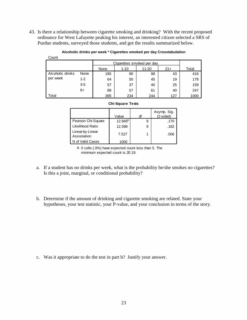
43. Is there a relationship between cigarette smoking and drinking? With the recent proposed

ordinance for West Lafayette peaking his interest, an interested citizen selected a SRS of

Purdue students, surveyed those students, and got the results summarized below.

Alcoholic drinks per week * Cigarettes smoked per day Crosstabulation Alcoholic drinks per week * Cigarettes smoked per day Crosstabulation

Count

185 90 98 43 416

64 50 45 19 178

57 37 40 25 159

89 57 61 40 247

395 234 244 127 1000

None

1-2

3-5

6+

Alcoholic drinks

per week

Total

None 1-10 11-20 21+

Cigarettes smoked per day

Total

Chi-Square Tests

12.845a 9 .170

12.598 9 .182

7.527 1 .006

1000

Pearson Chi-Square

Likelihood Ratio

Linear-by-Linear

Association

N of Valid Cases

Value df

Asymp. Sig.

(2-sided)

0 cells (.0%) have expected count less than 5. The

minimum expected count is 20.19.

a.

a. If a student has no drinks per week, what is the probability he/she smokes no cigarettes?

Is this a joint, marginal, or conditional probability?

b. Determine if the amount of drinking and cigarette smoking are related. State your

hypotheses, your test statistic, your P-value, and your conclusion in terms of the story.

c. Was it appropriate to do the test in part b? Justify your answer.