Stat 112: Notes 2

• This class: Start Section 3.3.

• Thursday’s class: Finish Section 3.3.

• I will e-mail and post on the web site the first homework tonight. It will be due next Thursday.

Father and Son’s Heights• Francis Galton was interested in the

relationship between – Y=son’s height– X=father’s height

• Galton surveyed 952 father-son pairs in 19th Century England.

• Data is in Galton.JMP

Bivariate Fit of sons ht By father ht

61

63

65

67

69

71

73

75

sons

ht

63 64 65 66 67 68 69 70 71 72 73 74

father ht

Simple Linear Regression Model Bivariate Fit of sons ht By father ht

61

63

65

67

69

71

73

75

sons

ht

63 64 65 66 67 68 69 70 71 72 73 74

father ht

Linear Fit sons ht = 26.455559 + 0.6115222 father ht Summary of Fit RSquare 0.177196 RSquare Adj 0.17633 Root Mean Square Error 2.356912

The mean of son’s height given father’s height is estimated to increase 1 0.61b inches for each

one inch increase in father’s height. The average absolute error from using the regression line to predict a son’s height based on the father’s height is about equal to the RMSE = 2.36.

Sample vs. Population

• We can view the data – -- as a sample from a population.

• Our goal is to learn about the relationship between X and Y in the population: – We don’t care about how father’s heights and son’s

heights are related in the particular 952 men sampled but among all fathers and sons.

– From Notes 1, we don’t care about the relationship between tracks counted and the density of deer for the particular sample, but the relationship among the population of all tracks; this enables to predict in the future the density of deer from the number of tracks counted.

1 1( , ), , ( , )n nX Y X Y

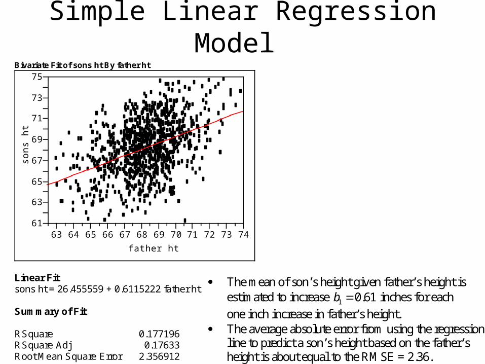
Simple Linear Regression ModelThe simple linear regression model:

0 1i i iY x e .

The ie are called disturbances and it is assumed that 1. Linearity assumption: The conditional expected value

of the disturbances given ix is zero, ( ) 0iE e , for

each i. This implies that 0 1( | )E Y x x so that the expected value of Y given X is a linear function of X.

2. Constant variance: assumption: The disturbances

ie are assumed to all have the same variance 2 .

3. Normality assumption: The disturbances ie are assumed to have a normal distribution.

4. Independence assumption: The disturbances ie are assumed to be independent. This is an assumption that is most important when the data are gathered over time. When the data are cross-sectional (that is, gathered at the same point in time for different individual units), this is typically not an assumption of concern.

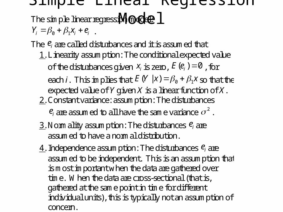
Checking the AssumptionsSimple Linear Regression Model for Population:

0 1i i iY x e . Before making any inferences using the simple linear regression model, we need to check the assumptions:

Based on the data 1 1 ,( , ), , ( )n nX Y X Y ,

1. We estimate 0 and 1 by the least squares estimates

0b and 1b .

2. We estimate the disturbances ie by the residuals

0 1ˆˆ ( | ) ( )i i i i ie Y E Y X Y b b X .

3. We check if the residuals approximate satisfy

(1) Linearity: ˆ( ) 0iE e for all range of iX .

(2) Constant Variance: ˆ( )iVar e constant for all

range of iX .

(3) Normality: ie are approximately normally distributed.

(4) Independence : ie are independent (only worry about for time series data).

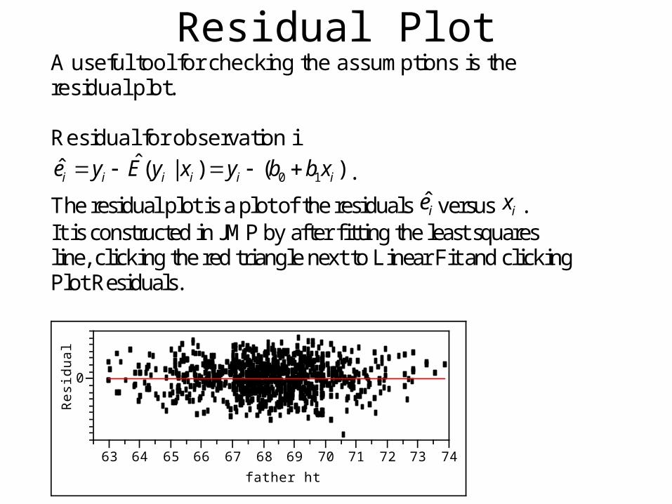
Residual Plot A useful tool for checking the assumptions is the residual plot. Residual for observation i

0 1ˆˆ ( | ) ( )i i i i i ie y E y x y b b x .

The residual plot is a plot of the residuals ie versus ix . It is constructed in JMP by after fitting the least squares line, clicking the red triangle next to Linear Fit and clicking Plot Residuals.

0

Res

idua

l

63 64 65 66 67 68 69 70 71 72 73 74

father ht

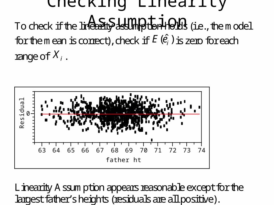
Checking Linearity Assumption

To check if the linearity assumption holds (i.e., the model

for the mean is correct), check if ˆ( )iE e is zero for each

range of iX .

0

Res

idua

l

63 64 65 66 67 68 69 70 71 72 73 74

father ht

Linearity Assumption appears reasonable except for the largest father’s heights (residuals are all positive).

Violation of LinearityFor a sample of McDonald’s restaurants Y=Revenue of Restaurant X=Mean Age of Children in Neighborhood of Restaurant Bivariate Fit of Revenue By Age

800

900

1000

1100

1200

1300

Rev

enue

2.5 5.0 7.5 10.0 12.5 15.0

Age

-200

-100

0

100

200

300

Res

idua

l2.5 5.0 7.5 10.0 12.5 15.0

Age

The mean of the residuals is negative for small and large ages and positive for large ages – linearity appears to be violated (we will see what to do when linearity is violated in Chapter 5).

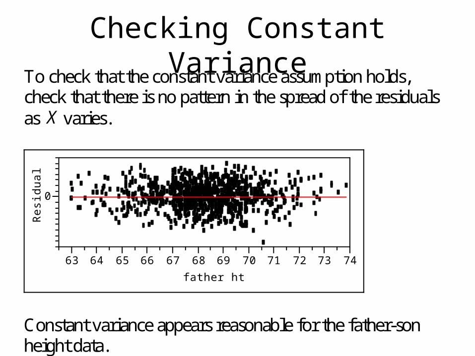
Checking Constant VarianceTo check that the constant variance assumption holds, check that there is no pattern in the spread of the residuals as X varies.

0

Res

idua

l

63 64 65 66 67 68 69 70 71 72 73 74

father ht

Constant variance appears reasonable for the father-son height data.

Checking NormalityFor checking normality, we can look at whether the overall distribution of the residuals looks approximately normal by making a histogram of the residuals. Save the residuals by clicking the red triangle next to Linear Fit after Fit Line and then clicking Save Residuals. Then click Analyze, Distribution and put the saved residuals column into Y, Columns. The histogram should be approximately bell shaped if the normality assumption holds. Distributions Residuals sons ht

-9 -8 -7 -6 -5 -4 -3 -2 -1 0 1 2 3 4 5 6

The residuals from the father-son height data have approximately a bell shaped histogram although there is some indication of skewness to the left. The normality assumption seems reasonable. We will look at more formal tools for assessing normality in Chapter 6.

InferencesSimple Linear Regression Model for Population:

0 1i i iY x e .

Data: 1 1( , ), , ( , )n nX Y X Y .

The least squares estimates 0b and 1b will typically not be

exactly equal to the true 0 and 1 .

Inferences: Draw conclusions about 0 and 1 based on the

data 1 1( , ), , ( , )n nX Y X Y .

Point Estimates: Best estimates of 0 and 1 . Confidence intervals: Ranges of plausible values of

0 and 1 . Hypothesis tests: Test whether it is plausible that

0 and 1 equal certain values.

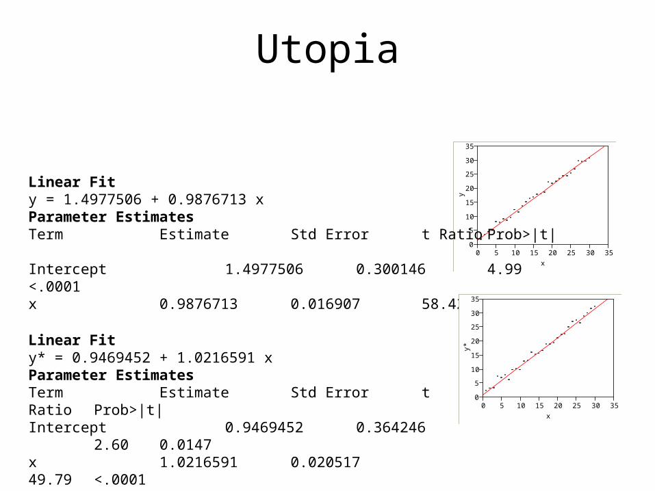
Sampling Distribution of b0,b1

• Utopia.JMP contains simulations of pairs and from a simple

linear regression model with • Notice the difference in the estimated

coefficients from the y’s and y*’s.• The sampling distribution of describes the

probability distribution of the estimates over repeated samples from the simple linear regression model with fixed.

),(,),,( 11 nn yxyx ),(,),,( **11 nn yxyx

1,1,1 210 e

10 ,bb

),,( 1 nyy ),,( 1 nxx

10 ,bb

Utopia

0

5

10

15

20

25

30

35

y

0 5 10 15 20 25 30 35

x

Linear Fity = 1.4977506 + 0.9876713 xParameter EstimatesTerm Estimate Std Error t Ratio Prob>|t|Intercept 1.4977506 0.300146 4.99 <.0001x 0.9876713 0.016907 58.42 <.0001

Linear Fity* = 0.9469452 + 1.0216591 xParameter EstimatesTerm Estimate Std Error t Ratio Prob>|t|Intercept 0.9469452 0.364246 2.60 0.0147x 1.0216591 0.020517 49.79 <.0001

0

5

10

15

20

25

30

35

y*

0 5 10 15 20 25 30 35

x

Sampling distributions

• Sampling distribution of – – – Sampling distribution is normally distributed.

• Sampling distribution of – –

– Sampling distribution is normally distributed.– Even if the normality assumption fails and the errors e are not

normal, the sampling distributions of are still approximately normal if n>30.

0b

00)( bE)

)1(

1()( 2

22

0

x

esn

x

nbVar

1b

11)( bE

2

2

1)1(

)(x

e

snbVar

0 1,b b

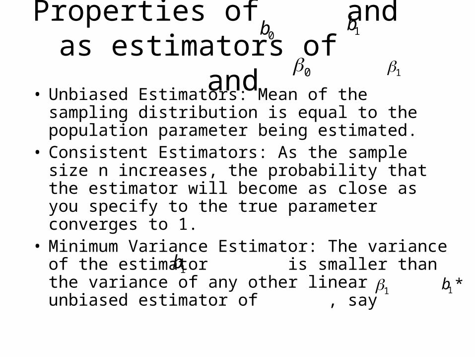
Properties of and as estimators of and

• Unbiased Estimators: Mean of the sampling distribution is equal to the population parameter being estimated.

• Consistent Estimators: As the sample size n increases, the probability that the estimator will become as close as you specify to the true parameter converges to 1.

• Minimum Variance Estimator: The variance of the estimator is smaller than the variance of any other linear unbiased estimator of , say

0b 1b

0 1

1b

1 *1b