Embed Size (px)
Citation preview

Stat 110 Strategic Practice 11, Fall 2011
Prof. Joe Blitzstein (Department of Statistics, Harvard University)
1 Law of Large Numbers, Central Limit Theorem
1. Give an intuitive argument that the Central Limit Theorem implies the WeakLaw of Large Numbers, without worrying about the di↵erent forms of conver-gence; then briefly explain how the forms of convergence involved are di↵erent.
2. (a) Explain why the Pois(n) distribution is approximately Normal if n is a largepositive integer (specifying what the parameters of the Normal are).
(b) Stirling’s formula is an amazingly accurate approximation for factorials:
n! ⇡p2⇡n
⇣n
e
⌘n,
where in fact the ratio of the two sides goes to 1 as n ! 1. Use (a) to give aquick heuristic derivation of Stirling’s formula by using a Normal approximationto the probability that a Pois(n) r.v. is n, with the continuity correction: firstwrite P (N = n) = P (n� 1
2 < N < n+ 12), where N ⇠ Pois(n).
3. Let T1, T2, . . . be i.i.d. Student-t r.v.s with m � 3 degrees of freedom. Findconstants an and bn (in terms of m and n) such that an(T1+T2+ · · ·+Tn� bn)converges to N (0, 1) in distribution as n ! 1.
4. Let X1, X2, . . . be i.i.d. positive random variables with mean 2. Let Y1, Y2, . . .
be i.i.d. positive random variables with mean 3. Show that
X1 +X2 + · · ·+Xn
Y1 + Y2 + · · ·+ Yn! 2
3
with probability 1. Does it matter whether the Xi are independent of the Yj?
5. Let f be a complicated function whose integralR b
a f(x)dx we want to ap-proximate. Assume that 0 f(x) c. Let A be the rectangle in the(x, y)-plane given by a x b and 0 y c. Pick i.i.d. uniform points(X1, Y1), (X2, Y2), . . . , (Xn, Yn) in the rectangle A.
How would you use these random points to approximate the integral? (Thisis an example of a Monte Carlo method.) Show that the estimate converges tothe true value of the integral as n ! 1. Hint: look at whether each point isin the area below the curve y = f(x).
1

2 Multivariate Normal
1. Show that if (X1, X2, X3) is Multivariate Normal, then so is the subvector(X1, X2).
2. Is it true that if X = (X1, . . . , Xn) and Y = (Y1, . . . , Ym) are MultivariateNormals with X independent of Y, then the “concatenated” random vectorW = (X1, . . . , Xn, Y1, . . . , Ym) is Multivariate Normal?
3. Let (X, Y ) be Bivariate Normal, with X, Y ⇠ N (0, 1) (marginally) and correla-tion ⇢, where �1 < ⇢ < 1. Find a, b, c, d (in terms of ⇢) such that Z = aX+bY
and W = cX + dY are independent N (0, 1).
4. Let X1, . . . , Xn be i.i.d. N (µ, �2), with n � 2. Let X̄n be the sample mean,and let S2
n = 1n�1
Pnj=1(Xj � X̄n)2 (this is called the sample variance, and is an
unbiased estimator for �2). Show that X̄n and S
2n are independent by applying
MVN ideas and results to the vector (X̄n, X1 � X̄n, . . . , Xn � X̄n).
3 Markov Chains
1. Let X0, X1, X2 . . . be a Markov chain. Show that X0, X2, X4, X6, . . . is also aMarkov chain, and explain why this makes sense intuitively.
Let Yn = X2n; we need to show Y0, Y1, . . . is a Markov chain. By the definitionof a Markov chain, we know thatX2n+1, X2n+2, . . . (“the future” if we define the“present” to be time 2n) is conditionally independent ofX0, X1, . . . , X2n�2, X2n�1
(“the past”), given X2n. So given Yn, we have that Yn+1, Yn+2, . . . is condition-ally independent of Y0, Y1, . . . , Yn�1. Thus,
P (Yn+1 = y|Y0 = y0, . . . , Yn = yn) = P (Yn+1 = y|Yn = yn).
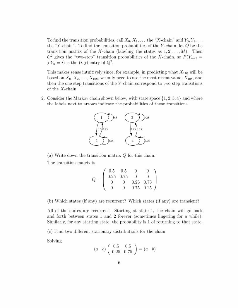
2. Consider the Markov chain shown below, with state space {1, 2, 3, 4} and wherethe labels next to arrows indicate the probabilities of those transitions.
(a) Write down the transition matrix Q for this chain.
(b) Which states (if any) are recurrent? Which states (if any) are transient?
(c) Find two di↵erent stationary distributions for the chain.
2
1 0.5
2
0.5 0.25
0.75
3 0.25
4
0.75 0.75
0.25
3. A cat and a mouse move independently back and forth between two rooms.At each time step, the cat moves from the current room to the other roomwith probability 0.8. Starting from Room 1, the mouse moves to Room 2 withprobability 0.3 (and remains otherwise). Starting from Room 2, the mousemoves to Room 1 with probability 0.6 (and remains otherwise).
(a) Find the stationary distributions of the cat chain and of the mouse chain.
(b) Note that there are 4 possible (cat, mouse) states: both in Room 1, cat inRoom 1 and mouse in Room 2, cat in Room 2 and mouse in Room 1, and bothin Room 2. Number these cases 1,2,3,4 respectively, and let Zn be the numberof the current (cat, mouse) state at time n. Is Z0, Z1, Z2, . . . a Markov chain?
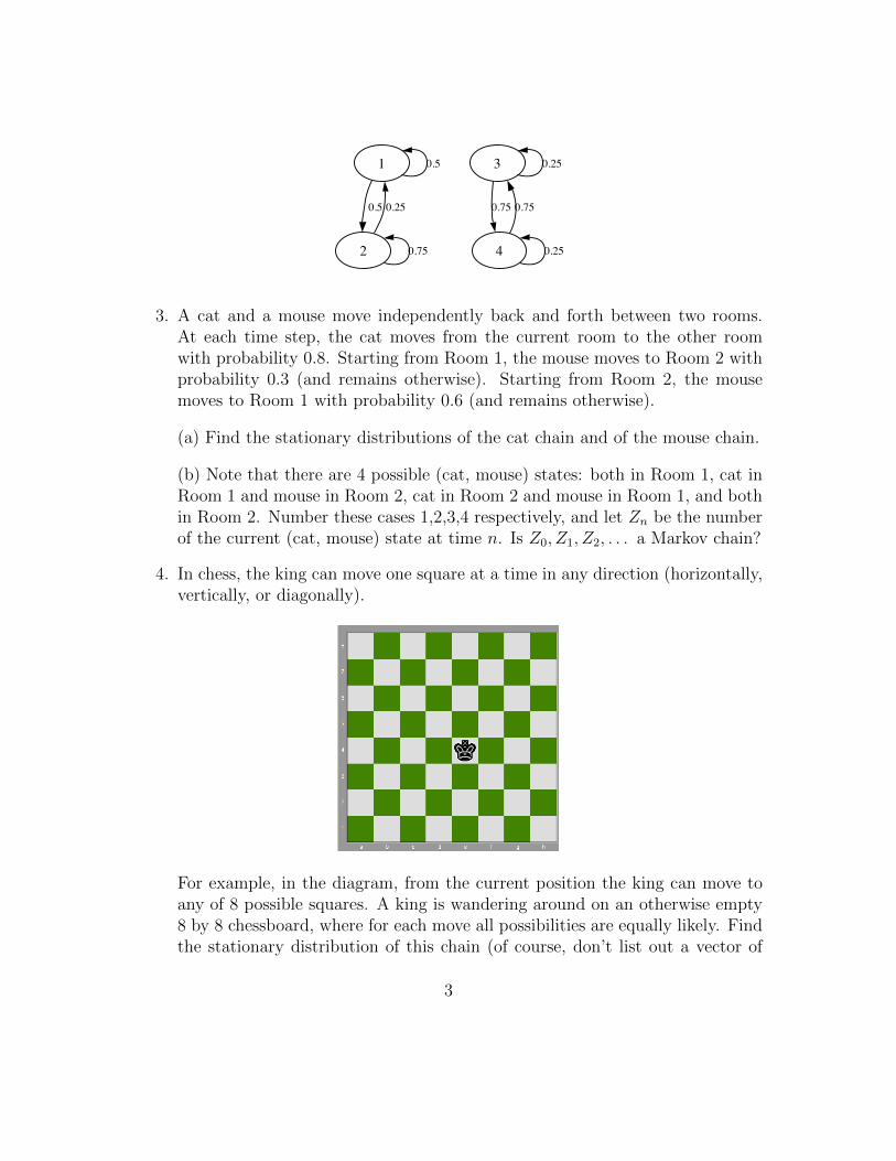
4. In chess, the king can move one square at a time in any direction (horizontally,vertically, or diagonally).
For example, in the diagram, from the current position the king can move toany of 8 possible squares. A king is wandering around on an otherwise empty8 by 8 chessboard, where for each move all possibilities are equally likely. Findthe stationary distribution of this chain (of course, don’t list out a vector of
3
length 64 explicitly! Classify the 64 squares into “types” and say what thestationary probability is for a square of each type).
5. Markov chains have recently been applied to code-breaking; this problem willconsider one way in which this can be done. A substitution cipher is a permu-tation g of the letters from a to z, where a message is enciphered by replacingeach letter ↵ by g(↵). For example, if g is the permutation given by
abcdefghijklmnopqrstuvwxyz
zyxwvutsrqponmlkjihgfedcba
where the second row lists the values g(a), g(b), . . . , g(z), then we would enci-pher the word “statistics” as “hgzgrhgrxh”. The state space is all 26! ⇡ 4 ·1026permutations of the letters a through z.
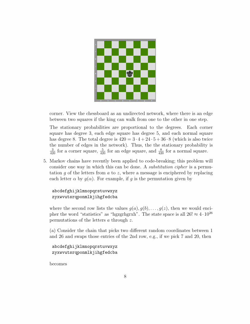
(a) Consider the chain that picks two di↵erent random coordinates between 1and 26 and swaps those entries of the 2nd row, e.g., if we pick 7 and 20, then
abcdefghijklmnopqrstuvwxyz
zyxwvutsrqponmlkjihgfedcba
becomes
abcdefghijklmnopqrstuvwxyz
zyxwvugsrqponmlkjihtfedcba
Find the probability of going from a permutation g to a permutation h in onestep (for all g, h), and find the stationary distribution of this chain.
(b) Suppose we have a system that assigns a positive “score” s(g) to eachpermutation g (intuitively, this could be a measure of how likely it would be toget the observed enciphered text, given that g was the cipher used). Considerthe following Markov chain. Starting from any state g, generate a “proposal” h
using the chain from (a). If s(g) s(h), then go to h (i.e., accept the proposal).Otherwise, flip a coin with probability s(h)/s(g) of Heads. If Heads, go to h
(i.e., accept the proposal); if Tails, stay at g. Show that this chain is reversibleand has stationary distribution proportional to the list of all scores s(g).
Hint: for g 6= h, let q(g, h) be the probability of going from g to h in one step,and show that s(g)q(g, h) = s(h)q(h, g). To compute q(g, h), note that it is theprobability of proposing h when at g, times the probability of accepting theproposal.
4
Stat 110 Strategic Practice 11 Solutions, Fall 2011
Prof. Joe Blitzstein (Department of Statistics, Harvard University)
1 Law of Large Numbers, Central Limit Theorem
1. Give an intuitive argument that the Central Limit Theorem implies the WeakLaw of Large Numbers, without worrying about the di↵erent forms of conver-gence; then briefly explain how the forms of convergence involved are di↵erent.
Let X1, X2, . . . be i.i.d. with mean µ and variance �
2. The CLT says thatpn
�
(X̄n � µ) ! N (0, 1)
in distribution. Sincepn goes to infinity, it makes sense that X̄n�µ should go
to 0, to preventpn(X̄n � µ) from exploding. The CLT is more informative in
the sense that it gives the shape of the distribution of the sample mean (afterstandardization), and gives information about the rate at which the samplemean goes to the true mean (replacing
pn by a di↵erent power of n, the
expression would go to 0 or 1 rather than to a Normal distribution).
On the other hand, the CLT is a statement about convergence in distribution
(i.e., the distribution of the r.v. on the left goes to the standard Normal distri-bution), while the Weak Law of Large Numbers says that the r.v. X̄n will beextremely close to µ with extremely high probability, for n large enough.
2. (a) Explain why the Pois(n) distribution is approximately Normal if n is a largepositive integer (specifying what the parameters of the Normal are).
Let Sn = X1 + · · · +Xn, with X1, X2, . . . i.i.d. ⇠ Pois(1). Then Sn ⇠ Pois(n)and for n large, Sn is approximately N (n, n) by the CLT.
(b) Stirling’s formula is an amazingly accurate approximation for factorials:
n! ⇡p2⇡n
⇣n
e
⌘n,
where in fact the ratio of the two sides goes to 1 as n ! 1. Use (a) to give aquick heuristic derivation of Stirling’s formula by using a Normal approximationto the probability that a Pois(n) r.v. is n, with the continuity correction: firstwrite P (N = n) = P (n� 1
2 < N < n+ 12), where N ⇠ Pois(n).
1
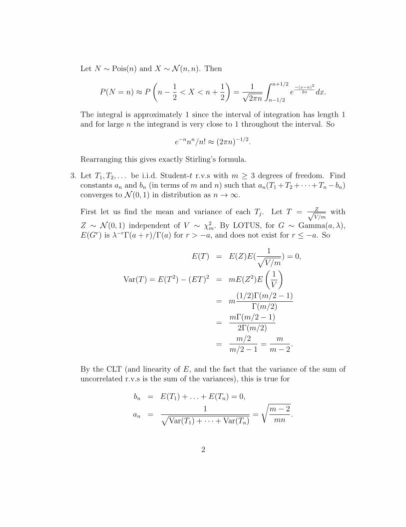
Let N ⇠ Pois(n) and X ⇠ N (n, n). Then
P (N = n) ⇡ P
✓n� 1
2< X < n+
1
2
◆=
1p2⇡n
Z n+1/2
n�1/2
e
�(x�n)2
2ndx.
The integral is approximately 1 since the interval of integration has length 1and for large n the integrand is very close to 1 throughout the interval. So
e
�nn
n/n! ⇡ (2⇡n)�1/2
.
Rearranging this gives exactly Stirling’s formula.
3. Let T1, T2, . . . be i.i.d. Student-t r.v.s with m � 3 degrees of freedom. Findconstants an and bn (in terms of m and n) such that an(T1+T2+ · · ·+Tn� bn)converges to N (0, 1) in distribution as n ! 1.
First let us find the mean and variance of each Tj. Let T = ZpV/m
with
Z ⇠ N (0, 1) independent of V ⇠ �
2m. By LOTUS, for G ⇠ Gamma(a,�),
E(Gr) is ��r�(a+ r)/�(a) for r > �a, and does not exist for r �a. So
E(T ) = E(Z)E(1pV/m
) = 0,
Var(T ) = E(T 2)� (ET )2 = mE(Z2)E
✓1
V
◆
= m
(1/2)�(m/2� 1)
�(m/2)
=m�(m/2� 1)
2�(m/2)
=m/2
m/2� 1=
m
m� 2.
By the CLT (and linearity of E, and the fact that the variance of the sum ofuncorrelated r.v.s is the sum of the variances), this is true for
bn = E(T1) + . . .+ E(Tn) = 0,
an =1p
Var(T1) + · · ·+Var(Tn)=
rm� 2
mn
.
2
4. Let X1, X2, . . . be i.i.d. positive random variables with mean 2. Let Y1, Y2, . . .
be i.i.d. positive random variables with mean 3. Show that
X1 +X2 + · · ·+Xn
Y1 + Y2 + · · ·+ Yn! 2
3
with probability 1. Does it matter whether the Xi are independent of the Yj?
By the Law of Large Numbers, X1+X2+···+Xn
n ! 2 with probability 1 andY1+Y2+···+Y
n
n ! 3 with probability 1, as n ! 1. Note that if two events A
and B both have probability 1, then the event A\B also has probability 1. Sowith probability 1, both the convergence involving the Xi and the convergenceinvolving the Yj occur. Therefore,
X1 +X2 + · · ·+Xn
Y1 + Y2 + · · ·+ Yn=
(X1 +X2 + · · ·+Xn)/n
(Y1 + Y2 + · · ·+ Yn)/n! 2
3with probability 1
as n ! 1. It was not necessary to assume that the Xi are independent of theYj because of the pointwise with probability 1 convergence.
5. Let f be a complicated function whose integralR b
a f(x)dx we want to ap-proximate. Assume that 0 f(x) c. Let A be the rectangle in the(x, y)-plane given by a x b and 0 y c. Pick i.i.d. uniform points(X1, Y1), (X2, Y2), . . . , (Xn, Yn) in the rectangle A.
How would you use these random points to approximate the integral? (Thisis an example of a Monte Carlo method.) Show that the estimate converges tothe true value of the integral as n ! 1. Hint: look at whether each point isin the area below the curve y = f(x).
Let B be the region under the curve y = f(x) (and above the x axis) fora x b, so the desired integral is the area of region B. Define indicator r.v.sI1, . . . , In by letting Ij = 1 if Xj is in B and Ij = 0 otherwise. Let µ = E(I1).In terms of areas, µ is the ratio of the area of B to the area of the rectangle A:
µ = E(Ij) = P (Ij = 1) =
R b
a f(x)dx
c(b� a).
We can estimate µ using 1n
Pnj=1 Ij, and then estimate the desired integral by
Z b
a
f(x)dx ⇡ c(b� a)1
n
nX
j=1
Ij.
Since the Ij are i.i.d. with mean µ, it follows from the Law of Large Numbersthat with probability 1, the estimate converges to the true value of the integral.
3
2 Multivariate Normal
1. Show that if (X1, X2, X3) is Multivariate Normal, then so is the subvector(X1, X2).
Any linear combination t1X1 + t2X2 can be thought of as a linear combinationof X1, X2, X3 (where the coe�cient of X3 is 0), so t1X1 + t2X2 is Normal forall t1, t2, which shows that (X1, X2) is MVN.
2. Is it true that if X = (X1, . . . , Xn) and Y = (Y1, . . . , Ym) are MultivariateNormals with X independent of Y, then the “concatenated” random vectorW = (X1, . . . , Xn, Y1, . . . , Ym) is Multivariate Normal?
Yes, since any linear combination s1X1+· · ·+snXn+t1Y1+· · ·+tmYm is Normal,because s1X1 + · · ·+ snXn and t1Y1 + · · ·+ tmYm are Normal (by definition ofX and Y being MVN) and are independent, so their sum is Normal.
3. Let (X, Y ) be Bivariate Normal, with X, Y ⇠ N (0, 1) (marginally) and correla-tion ⇢, where �1 < ⇢ < 1. Find a, b, c, d (in terms of ⇢) such that Z = aX+bY
and W = cX + dY are independent N (0, 1).
We need to find a, b, c, d such that
Cov(Z,W ) = Cov(aX + bY, cX + dY )
= Cov(aX, cX) + Cov(bY, cX) + Cov(aX, dY ) + Cov(bY, dY )
= acVar(X) + (bc+ ad)Cov(X, Y ) + dbVar(Y )
= ac+ (bc+ ad)⇢+ db = 0, (1)
Var(Z) = Cov(aX + bY, aX + bY )
= a
2Var(X) + 2abCov(X, Y ) + b
2Var(Y )
= a
2 + 2ab⇢+ b
2 = 1, (2)
Var(W ) = c
2 + 2cd⇢+ d
2 = 1. (3)
Since uncorrelated implies independent within a Multivariate Normal, if wecan solve these equations then Z and W are as desired. These are 3 equationsin 4 unknowns, so there may be many solutions; let us simplify by looking fora solution with a = 1. Then by (2), 2b⇢ + b
2 = b(2⇢ + b) = 0, so b = 0 orb = �2⇢. Trying the possibility b = 0, we then have c = �d⇢ by (1). Pluggingthis into equation (3) gives us
(�d⇢)2 + 2(�d⇢)d⇢+ d
2 = d
2(1� ⇢
2) = 1,
4
which yields d = ±1/p
1� ⇢
2. So if we let a = 1, b = 0, c = �⇢/
p1� ⇢
2, and
d = 1/p
1� ⇢
2, then Z = aX + bY and W = cX + dY are i.i.d. N (0, 1).
4. Let X1, . . . , Xn be i.i.d. N (µ, �2), with n � 2. Let X̄n be the sample mean,and let S2
n = 1n�1
Pnj=1(Xj � X̄n)2 (this is called the sample variance, and is an
unbiased estimator for �2). Show that X̄n and S
2n are independent by applying
MVN ideas and results to the vector (X̄n, X1 � X̄n, . . . , Xn � X̄n).
The vector X̄n, X1 � X̄n, . . . , Xn � X̄n) is MVN since any linear combinationof its components can be written as a linear combination of X1, . . . , Xn. Nowcompute the covariance of X̄n with Xj � X̄n:
Cov(X̄n, Xj � X̄n) = E(X̄n(Xj � X̄n)).
This can be found by expanding it out, but a faster way is to use Adam’s Lawto write it as
E(E(X̄n(Xj � X̄n)|X̄n)) = E(X̄n(E(Xj � X̄n)|X̄n)).
But this is 0 since E(Xj � X̄n|X̄n) = E(Xj|X̄n)� E(X̄n|X̄n) = X̄n � X̄n = 0,using the idea of Problem 2 from the Penultimate Homework. Therefore, X̄n
is uncorrelated with (X1 � X̄n, . . . , Xn � X̄n) (i.e., it is uncorrelated with eachcomponent of this vector). Since within a MVN it is true that uncorrelatedimplies independent, we have that X̄n is independent of (X1�X̄n, . . . , Xn�X̄n).Thus, X̄n is independent of S2
n.
3 Markov Chains
1. Let X0, X1, X2 . . . be a Markov chain. Show that X0, X2, X4, X6, . . . is also aMarkov chain, and explain why this makes sense intuitively.
Let Yn = X2n; we need to show Y0, Y1, . . . is a Markov chain. By the definitionof a Markov chain, we know thatX2n+1, X2n+2, . . . (“the future” if we define the“present” to be time 2n) is conditionally independent ofX0, X1, . . . , X2n�2, X2n�1
(“the past”), given X2n. So given Yn, we have that Yn+1, Yn+2, . . . is condition-ally independent of Y0, Y1, . . . , Yn�1. Thus,
P (Yn+1 = y|Y0 = y0, . . . , Yn = yn) = P (Yn+1 = y|Yn = yn).
5
To find the transition probabilities, callX0, X1, . . . the “X-chain” and Y0, Y1, . . .
the “Y -chain”. To find the transition probabilities of the Y -chain, let Q be thetransition matrix of the X-chain (labeling the states as 1, 2, . . . ,M). ThenQ
2 gives the “two-step” transition probabilities of the X-chain, so P (Yn+1 =j|Yn = i) is the (i, j) entry of Q2.
This makes sense intuitively since, for example, in predicting what X110 will bebased on X0, X2, . . . , X108, we only need to use the most recent value, X108, andthen the one-step transitions of the Y -chain correspond to two-step transitionsof the X-chain.
2. Consider the Markov chain shown below, with state space {1, 2, 3, 4} and wherethe labels next to arrows indicate the probabilities of those transitions.
1 0.5
2
0.5 0.25
0.75
3 0.25
4
0.75 0.75
0.25
(a) Write down the transition matrix Q for this chain.
The transition matrix is
Q =
0
BB@
0.5 0.5 0 00.25 0.75 0 00 0 0.25 0.750 0 0.75 0.25
1
CCA
(b) Which states (if any) are recurrent? Which states (if any) are transient?
All of the states are recurrent. Starting at state 1, the chain will go backand forth between states 1 and 2 forever (sometimes lingering for a while).Similarly, for any starting state, the probability is 1 of returning to that state.
(c) Find two di↵erent stationary distributions for the chain.
Solving
(a b)
✓0.5 0.50.25 0.75
◆= (a b)
6
(c d)
✓0.25 0.750.75 0.25
◆= (c d)
shows that (a, b) = (1/3, 2/3), and (c, d) = (1/2, 1/2) are stationary distribu-tions on the 1, 2 chain and on the 3, 4 chain respectively, viewed as separatechains. It follows that (1/3, 2/3, 0, 0) and (0, 0, 1/2, 1/2) are both stationary forQ (as is any mixture p(1/3, 2/3, 0, 0) + (1� p)(0, 0, 1/2, 1/2) with 0 p 1).
3. A cat and a mouse move independently back and forth between two rooms.At each time step, the cat moves from the current room to the other roomwith probability 0.8. Starting from Room 1, the mouse moves to Room 2 withprobability 0.3 (and remains otherwise). Starting from Room 2, the mousemoves to Room 1 with probability 0.6 (and remains otherwise).
(a) Find the stationary distributions of the cat chain and of the mouse chain.
For the cat Markov chain, the stationary distribution is (1/2, 1/2) by symmetry.For the mouse Markov chain: solving sQ = s and normalizing yields (2/3, 1/3).
(b) Note that there are 4 possible (cat, mouse) states: both in Room 1, cat inRoom 1 and mouse in Room 2, cat in Room 2 and mouse in Room 1, and bothin Room 2. Number these cases 1,2,3,4 respectively, and let Zn be the numberof the current (cat, mouse) state at time n. Is Z0, Z1, Z2, . . . a Markov chain?
Yes, it is a Markov chain. Given the current (cat, mouse) state, the past historyof where the cat and mouse were previously are irrelevant for computing theprobabilities of what the next state will be.
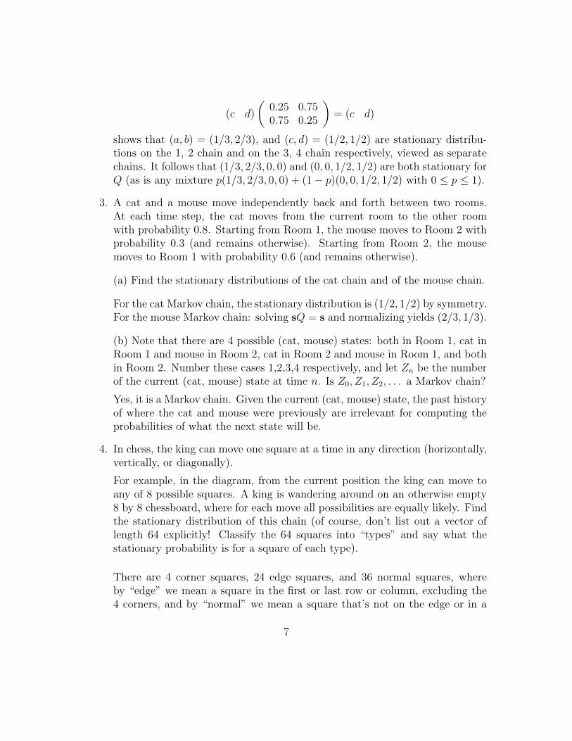
4. In chess, the king can move one square at a time in any direction (horizontally,vertically, or diagonally).
For example, in the diagram, from the current position the king can move toany of 8 possible squares. A king is wandering around on an otherwise empty8 by 8 chessboard, where for each move all possibilities are equally likely. Findthe stationary distribution of this chain (of course, don’t list out a vector oflength 64 explicitly! Classify the 64 squares into “types” and say what thestationary probability is for a square of each type).
There are 4 corner squares, 24 edge squares, and 36 normal squares, whereby “edge” we mean a square in the first or last row or column, excluding the4 corners, and by “normal” we mean a square that’s not on the edge or in a
7
corner. View the chessboard as an undirected network, where there is an edgebetween two squares if the king can walk from one to the other in one step.
The stationary probabilities are proportional to the degrees. Each cornersquare has degree 3, each edge square has degree 5, and each normal squarehas degree 8. The total degree is 420 = 3 · 4+24 · 5+36 · 8 (which is also twicethe number of edges in the network). Thus, the the stationary probability is3
420 for a corner square, 5420 for an edge square, and 8
420 for a normal square.
5. Markov chains have recently been applied to code-breaking; this problem willconsider one way in which this can be done. A substitution cipher is a permu-tation g of the letters from a to z, where a message is enciphered by replacingeach letter ↵ by g(↵). For example, if g is the permutation given by
abcdefghijklmnopqrstuvwxyz
zyxwvutsrqponmlkjihgfedcba
where the second row lists the values g(a), g(b), . . . , g(z), then we would enci-pher the word “statistics” as “hgzgrhgrxh”. The state space is all 26! ⇡ 4 ·1026permutations of the letters a through z.
(a) Consider the chain that picks two di↵erent random coordinates between 1and 26 and swaps those entries of the 2nd row, e.g., if we pick 7 and 20, then
abcdefghijklmnopqrstuvwxyz
zyxwvutsrqponmlkjihgfedcba
becomes
8
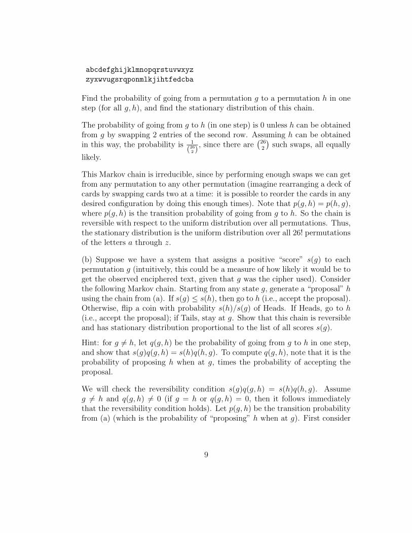
abcdefghijklmnopqrstuvwxyz
zyxwvugsrqponmlkjihtfedcba
Find the probability of going from a permutation g to a permutation h in onestep (for all g, h), and find the stationary distribution of this chain.
The probability of going from g to h (in one step) is 0 unless h can be obtainedfrom g by swapping 2 entries of the second row. Assuming h can be obtainedin this way, the probability is 1
(262 ), since there are
�262
�such swaps, all equally
likely.
This Markov chain is irreducible, since by performing enough swaps we can getfrom any permutation to any other permutation (imagine rearranging a deck ofcards by swapping cards two at a time: it is possible to reorder the cards in anydesired configuration by doing this enough times). Note that p(g, h) = p(h, g),where p(g, h) is the transition probability of going from g to h. So the chain isreversible with respect to the uniform distribution over all permutations. Thus,the stationary distribution is the uniform distribution over all 26! permutationsof the letters a through z.
(b) Suppose we have a system that assigns a positive “score” s(g) to eachpermutation g (intuitively, this could be a measure of how likely it would be toget the observed enciphered text, given that g was the cipher used). Considerthe following Markov chain. Starting from any state g, generate a “proposal” h
using the chain from (a). If s(g) s(h), then go to h (i.e., accept the proposal).Otherwise, flip a coin with probability s(h)/s(g) of Heads. If Heads, go to h
(i.e., accept the proposal); if Tails, stay at g. Show that this chain is reversibleand has stationary distribution proportional to the list of all scores s(g).
Hint: for g 6= h, let q(g, h) be the probability of going from g to h in one step,and show that s(g)q(g, h) = s(h)q(h, g). To compute q(g, h), note that it is theprobability of proposing h when at g, times the probability of accepting theproposal.
We will check the reversibility condition s(g)q(g, h) = s(h)q(h, g). Assumeg 6= h and q(g, h) 6= 0 (if g = h or q(g, h) = 0, then it follows immediatelythat the reversibility condition holds). Let p(g, h) be the transition probabilityfrom (a) (which is the probability of “proposing” h when at g). First consider
9
the case that s(g) s(h). Then q(g, h) = p(g, h) and
q(h, g) = p(h, g)s(g)
s(h)= p(g, h)
s(g)
s(h)= q(g, h)
s(g)
s(h),
so s(g)q(g, h) = s(h)q(h, g). Now consider the case that s(h) < s(g). By a sym-metrical argument (reversing the roles of g and h), we again have s(g)q(g, h) =s(h)q(h, g). Thus, the stationary probability of g is proportional to the scores(g).
The algorithm here is an example of the Metropolis algorithm, which is a pow-erful, general method of transmogrifying one Markov chain into a new Markovchain with a certain desired stationary distribution. This algorithm was namedone of the ten most important algorithms created in the 20th century!
10
Stat 110 Ultimate Homework, Fall 2011
Prof. Joe Blitzstein (Department of Statistics, Harvard University)
1. Each day, a very volatile stock rises 70% or drops 50% in price, with equalprobabilities (with di↵erent days independent). Let Xn be the stock price after ndays, starting from an initial value of X0 = 100.
(a) Explain why logXn is approximately Normal for n large, and state its parameters.
(b) What happens to E(Xn) as n ! 1?
(c) Use the Law of Large Numbers to find out what happens to Xn as n ! 1.
Hint: let Un be the number of days the stock rises up until time n.
2. Let Vn ⇠ �2n and Tn ⇠ tn for n 2 {1, 2, 3, . . . }.
(a) Find numbers an and bn such that an(Vn�bn) converges in distribution toN (0, 1).
(b) Show that T 2n/(n+ T 2
n) has a Beta distribution (without using calculus).
3. Let (X, Y ) be Bivariate Normal, with X and Y marginally N (0, 1) and withcorrelation ⇢ between X and Y .
(a) Use MGFs to show that if ⇢ = 0, then X and Y are independent (without quotingthe result from class about uncorrelated vectors within a Multivariate Normal). Youcan use the fact that the MGF E(esX+tY ) of a random vector (X, Y ) determines itsjoint distribution (if the MGF exists).
(b) Show that (X + Y,X � Y ) is also Bivariate Normal.
(c) Find the joint PDF of X + Y and X � Y (without using calculus).
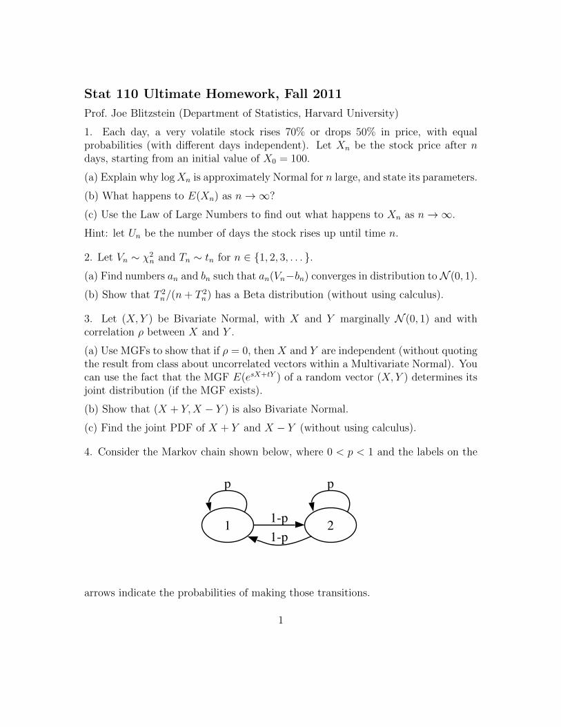
4. Consider the Markov chain shown below, where 0 < p < 1 and the labels on the
1
p
21-p
1-p
p
arrows indicate the probabilities of making those transitions.
1

(a) Write down the transition matrix Q for this chain.
(b) Find the stationary distribution of the chain.
(c) What is the limit of Qn as n ! 1?
5. In the Ehrenfest chain, there are two containers with a total ofM (distinguishable)particles, and transitions are done by choosing a random particle and moving it fromits current container into the other container. Initially (at time n = 0), all of theparticles are in the second container. Let Xn be the number of particles in the firstcontainer at time n (so X0 = 0 and the transition from Xn to Xn+1 is done asdescribed above). This is a Markov chain with state space {0, 1, . . . ,M}.
(a) Why is q(n)ii (i.e., the probability of being in state i after n steps, starting fromstate i) always 0 if n is odd?
(b) Show that (s0, s1, . . . , sM) with si =�Mi
�(12)
M is the stationary distribution. Whydoes this, which is a Binomial distribution, seem reasonable intuitively?
Hint: first show that siqij = sjqji.
6. Daenerys has three dragons: Drogon, Rhaegal, and Viserion. Each dragon in-dependently explores the world in search of tasty morsels. Let Xn, Yn, Zn be thelocations at time n of Drogon, Rhaegal, Viserion respectively, where time is assumedto be discrete and the number of possible locations is a finite number M . Their pathsX0, X1, X2, . . . ; Y0, Y1, Y2, . . . ; and Z0, Z1, Z2, . . . are independent Markov chainswith the same stationary distribution s. Each dragon starts out at a random lo-cation generated according to the stationary distribution.
(a) Let state 0 be “home” (so s0 is the stationary probability of the home state).Find the expected number of times that Drogon is at home, up to time 24, i.e., theexpected number of how many of X0, X1, . . . , X24 are state 0 (in terms of s0).
(b) If we want to track all 3 dragons simultaneously, we need to consider the vectorof positions, (Xn, Yn, Zn). There are M3 possible values for this vector; assumethat each is assigned a number from 1 to M3, e.g., if M = 2 we could encodethe states (0, 0, 0), (0, 0, 1), (0, 1, 0), . . . , (1, 1, 1) as 1, 2, 3, . . . , 8 respectively. Let Wn
be the number between 1 and M3 representing (Xn, Yn, Zn). Determine whetherW0,W1, . . . is a Markov chain.
(c) Given that all 3 dragons start at home at time 0, find the expected time it willtake for all 3 to be at home again at the same time.
7. Let G be a network (also called a graph); there are n nodes, and for each pair ofdistinct nodes, there either is or isn’t an edge joining them. We have a set of k colors,
2
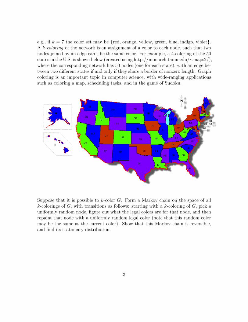
e.g., if k = 7 the color set may be {red, orange, yellow, green, blue, indigo, violet}.A k-coloring of the network is an assignment of a color to each node, such that twonodes joined by an edge can’t be the same color. For example, a 4-coloring of the 50states in the U.S. is shown below (created using http://monarch.tamu.edu/⇠maps2/),where the corresponding network has 50 nodes (one for each state), with an edge be-tween two di↵erent states if and only if they share a border of nonzero length. Graphcoloring is an important topic in computer science, with wide-ranging applicationssuch as coloring a map, scheduling tasks, and in the game of Sudoku.
Suppose that it is possible to k-color G. Form a Markov chain on the space of allk-colorings of G, with transitions as follows: starting with a k-coloring of G, pick auniformly random node, figure out what the legal colors are for that node, and thenrepaint that node with a uniformly random legal color (note that this random colormay be the same as the current color). Show that this Markov chain is reversible,and find its stationary distribution.
3
Stat 110 Ultimate Homework Solutions, Fall 2011
Prof. Joe Blitzstein (Department of Statistics, Harvard University)
1. Each day, a very volatile stock rises 70% or drops 50% in price, with equalprobabilities (with di↵erent days independent). Let X
n
be the stock price after n
days, starting from an initial value of X0 = 100.
(a) Explain why logXn
is approximately Normal for n large, and state its parameters.
We have Xn
= X0Y1Y2 . . . Yn
, where Yj
is 1.7 if the stock goes up on the jth day andY
j
is 0.5 otherwise (so Y
j
= X
j
/X
j�1). Taking logs,
log(Xn
) = log(X0) + log(Y1) + · · ·+ log(Yn
).
Let Zj
= log(Yj
). Then the Z
j
are i.i.d. with
P (Zn
= log(0.5)) = P (Zn
= log(1.7)) = 0.5,
E(Zn
) = log(0.85)/2 ⇡ �0.081,
Var(Zn
) ⇡ 0.374.
By the CLT, the distribution of Z1 + · · ·+ Z
n
, after standardization, converges to aNormal distribution. Thus, log(X
n
) is approximately Normal for large n, with
E(log (Xn
)) = log (X0) + nE(Z1) = log (100) + log(0.85)n/2 ⇡ log(100)� 0.081n,
Var(log (Xn
)) = nVar(Zn
) ⇡ 0.374n.
Alternatively, we can write X
n
= X0(0.5)n�Un(1.7)Un where U
n
⇠ Bin(n, 12) is thenumber of times the stock rises in the first n days. This gives
log(Xn
) = log(X0)� n log(2) + U
n
log(3.4),
which is just a location and scale transformation of Un
. By the CLT, Un
is approxi-mately N (n2 ,
n
4 ) for large n, so log(Xn
) is approximately Normal with the parametersas above for large n.
(b) What happens to E(Xn
) as n ! 1?
We have E(X1) = (170 + 50)/2 = 110. Similarly,
E(Xn+1|Xn
) =1
2(1.7X
n
) +1
2(0.5X
n
) = 1.1Xn
,
1
soE(X
n+1) = E(E(Xn+1|Xn
)) = 1.1E(Xn
).
Thus, E(Xn
) = 1.1nE(X0) goes to 1 as n ! 1.
(c) Use the Law of Large Numbers to find out what happens to X
n
as n ! 1.
Hint: let Un
be the number of days the stock rises up until time n.
Let Un
⇠ Bin(n, 12) be the number of times the stock rises in the first n days. Notethat even though E(X
n
) ! 1, if the stock goes up 70% one day and then drops50% the next day, then overall it has dropped 15% since 1.7 · 0.5 = 0.85. So X
n
willbe very small (for n large) if about half the time the stock rose 70% and about halfthe time the stock dropped 50%; and the Law of Large Numbers ensures that thiswill be the case! We have
X
n
= X0(0.5)n�Un(1.7)Un = X0
✓(3.4)Un/n
2
◆n
,
where we simplified in terms of Un
/n so that we can apply the Law of Large Numbers,which here gives that U
n
/n ! 0.5 with probability 1. But then (3.4)Un/n !p3.4 < 2
with probability 1, so X
n
! 0 with probability 1.
Paradoxically, EX
n
! 1 but Xn
! 0 with probability 1. With very high probabil-ity, the stock price will get very close to 0 since gaining 70% half the time while losing50% the other half of the time is very bad; but the expected price goes to 1 since onaverage each day the price is up 10% from the previous day. To gain more intuitionon this, consider a more extreme example, where a gambler starts with $100 andeach day either quadruples his or her money or loses the entire fortune, with equalprobabilities. Then on average the gambler’s wealth doubles each day, which soundsgood for that gambler until one notices that eventually there will be a day when thegambler goes broke. So the actual fortune goes to 0 with probability 1, whereas theexpected value goes to infinity due to tiny probabilities of getting extremely largeamounts of money (as in the St. Petersburg Paradox).
2. Let Vn
⇠ �
2n
and T
n
⇠ t
n
for n 2 {1, 2, 3, . . . }.(a) Find numbers a
n
and b
n
such that an
(Vn
�b
n
) converges in distribution toN (0, 1).
By definition of �2n
, we can take Vn
= Z
21+· · ·+Z
2n
, where Zj
⇠ N (0, 1) independently.We have E(Z2
1) = 1 and E(Z41) = 3, so Var(Z2
1) = 2. By the CLT, if we standardizeV
n
it will go to N (0, 1):
Z
21 + · · ·+ Z
2n
� np2n
! N (0, 1) in distribution.
2
So we can take a
n
= 1p2n, b
n
= n.
(b) Show that T 2n
/(n+ T
2n
) has a Beta distribution (without using calculus).
We can take T
n
= Z0/p
V
n
/n, with Z0 ⇠ N (0, 1) independent of Vn
. Then we haveT
2n
/(n+ T
2n
) = Z
20/(Z
20 + V
n
), with Z
20 ⇠ Gamma(1/2, 1/2), V
n
⇠ Gamma(n/2, 1/2).By the bank-post o�ce story, Z2
0/(Z20 + V
n
) ⇠ Beta(1/2, n/2).
3. Let (X, Y ) be Bivariate Normal, with X and Y marginally N (0, 1) and withcorrelation ⇢ between X and Y .
(a) Use MGFs to show that if ⇢ = 0, then X and Y are independent (without quotingthe result from class about uncorrelated vectors within a Multivariate Normal). Youcan use the fact that the MGF E(esX+tY ) of a random vector (X, Y ) determines itsjoint distribution (if the MGF exists).
Suppose that Cov(X, Y ) = 0. Then the MGF of (X, Y ) is
E(esX+tY ) = e
E(sX+tY )+ 12Var(sX+tY ) = e
12 (s
2+t
2) = e
12 s
2e
12 t
2.
For Z1, Z2 i.i.d. N (0, 1), the joint MGF is
E(esZ1+tZ2) = E(esZ1)E(etZ2) = e
12 s
2e
12 t
2,
the same as the above! Thus, X and Y are i.i.d. N (0, 1).
(b) Show that (X + Y,X � Y ) is also Bivariate Normal.
The linear combination s(X + Y ) + t(X � Y ) = (s+ t)X + (s� t)Y is also a linearcombination of X and Y , so it is Normal, which shows that (X+Y,X�Y ) is MVN.
(c) Find the joint PDF of X + Y and X � Y (without using calculus).
Since X+Y and X�Y are uncorrelated (as Cov(X+Y,X�Y ) = Var(X)�Var(Y ) =0) and (X+Y,X�Y ) is MVN, they are independent. Marginally, X+Y ⇠ N (0, 2+2⇢) and X � Y ⇠ N (0, 2� 2⇢). Thus, the joint PDF is
f(s, t) =1
4⇡p
1� ⇢
2e
� 14 (s
2/(1+⇢)+t
2/(1�⇢))
.
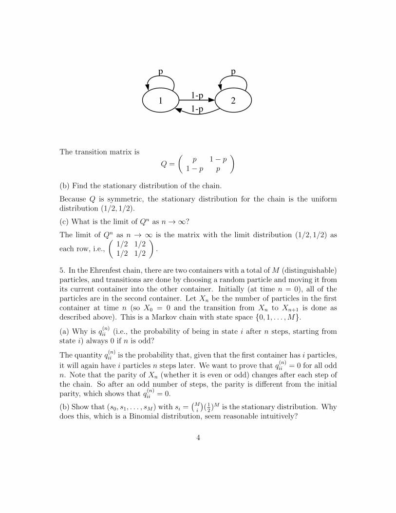
4. Consider the Markov chain shown below, where 0 < p < 1 and the labels on thearrows indicate the probabilities of making those transitions.
(a) Write down the transition matrix Q for this chain.
3
1
p
21-p
1-p
p
The transition matrix is
Q =
✓p 1� p
1� p p
◆
(b) Find the stationary distribution of the chain.
Because Q is symmetric, the stationary distribution for the chain is the uniformdistribution (1/2, 1/2).
(c) What is the limit of Qn as n ! 1?
The limit of Qn as n ! 1 is the matrix with the limit distribution (1/2, 1/2) as
each row, i.e.,
✓1/2 1/21/2 1/2
◆.
5. In the Ehrenfest chain, there are two containers with a total ofM (distinguishable)particles, and transitions are done by choosing a random particle and moving it fromits current container into the other container. Initially (at time n = 0), all of theparticles are in the second container. Let X
n
be the number of particles in the firstcontainer at time n (so X0 = 0 and the transition from X
n
to X
n+1 is done asdescribed above). This is a Markov chain with state space {0, 1, . . . ,M}.
(a) Why is q
(n)ii
(i.e., the probability of being in state i after n steps, starting fromstate i) always 0 if n is odd?
The quantity q
(n)ii
is the probability that, given that the first container has i particles,
it will again have i particles n steps later. We want to prove that q(n)ii
= 0 for all oddn. Note that the parity of X
n
(whether it is even or odd) changes after each step ofthe chain. So after an odd number of steps, the parity is di↵erent from the initialparity, which shows that q
(n)ii
= 0.
(b) Show that (s0, s1, . . . , sM) with s
i
=�M
i
�(12)
M is the stationary distribution. Whydoes this, which is a Binomial distribution, seem reasonable intuitively?
4
Hint: first show that si
q
ij
= s
j
q
ji
.
The Binomial distribution makes sense here since after running the Markov chain fora long time, each particle is about equally likely to be in either container, approxi-mately independently. To show that the stationary distribution is Binomial(M, 1/2),we will check the reversibility condition s
i
q
ij
= s
j
q
ji
.
Let si
=�M
i
�(12)
M , and check that si
q
ij
= s
j
q
ji
. If j = i+ 1 (for i < M), then
s
i
q
ij
=
✓M
i
◆(1
2)M
M � i
M
=M !
(M � i)!i!(1
2)M
M � i
M
=
✓M � 1
i
◆(1
2)M ,
s
j
q
ji
=
✓M
j
◆(1
2)M
j
M
=M !
(M � j)!j!(1
2)M
j
M
=
✓M � 1
j � 1
◆(1
2)M = s
i
q
ij
.
Similarly, if j = i � 1 (for i > 0), then s
i
q
ij
= s
j
q
ji
. For all other values of i, j,q
ij
= q
ji
= 0. Therefore, s is stationary.
6. Daenerys has three dragons: Drogon, Rhaegal, and Viserion. Each dragon in-dependently explores the world in search of tasty morsels. Let X
n
, Y
n
, Z
n
be thelocations at time n of Drogon, Rhaegal, Viserion respectively, where time is assumedto be discrete and the number of possible locations is a finite number M . Their pathsX0, X1, X2, . . . ; Y0, Y1, Y2, . . . ; and Z0, Z1, Z2, . . . are independent Markov chainswith the same stationary distribution s. Each dragon starts out at a random lo-cation generated according to the stationary distribution.
(a) Let state 0 be “home” (so s0 is the stationary probability of the home state).Find the expected number of times that Drogon is at home, up to time 24, i.e., theexpected number of how many of X0, X1, . . . , X24 are state 0 (in terms of s0).
By definition of stationarity, at each time Drogon has probability s0 of being at home.By linearity, the desired expected value is 25s0.
(b) If we want to track all 3 dragons simultaneously, we need to consider the vectorof positions, (X
n
, Y
n
, Z
n
). There are M
3 possible values for this vector; assumethat each is assigned a number from 1 to M
3, e.g., if M = 2 we could encodethe states (0, 0, 0), (0, 0, 1), (0, 1, 0), . . . , (1, 1, 1) as 1, 2, 3, . . . , 8 respectively. Let W
n
be the number between 1 and M
3 representing (Xn
, Y
n
, Z
n
). Determine whetherW0,W1, . . . is a Markov chain.
Yes, W0,W1, . . . is a Markov chain, since given the entire past history of the X, Y,
and Z chains, only the most recent information about the whereabouts of the dragonsshould be used in predicting their vector of locations. To show this algebraically, let
5
A
n
be the event {X0 = x0, . . . , Xn
= x
n
}, Bn
be the event {Y0 = y0, . . . , Yn
= y
n
},C
n
be the event {Z0 = z0, . . . , Zn
= z
n
}, and D
n
= A
n
\ B
n
\ C
n
. Then
P (Xn+1 = x, Y
n+1 = y, Z
n+1 = z|Dn
)
= P (Xn+1 = x|D
n
)P (Yn+1 = y|X
n+1 = x,D
n
)P (Zn+1 = z|X
n+1 = x, Y
n+1 = y,D
n
)
= P (Xn+1 = x|A
n
)P (Yn+1 = y|B
n
)P (Zn+1 = z|C
n
)
= P (Xn+1 = x|X
n
= x
n
)P (Yn+1 = y|Y
n
= y
n
)P (Zn+1 = z|Z
n
= z
n
).
(c) Given that all 3 dragons start at home at time 0, find the expected time it willtake for all 3 to be at home again at the same time.
The stationary probability for the W -chain of the state with Drogon, Rhaegal, Vis-erion being at locations x, y, z is s
x
s
y
s
z
, since if (Xn
, Y
n
, Z
n
) is drawn from this dis-tribution, then marginally each dragon’s location is distributed according to its sta-tionary distribution, so P (X
n+1 = x, Y
n+1 = y, Z
n+1 = z) = P (Xn+1 = x)P (Y
n+1 =y)P (Z
n+1 = z) = s
x
s
y
s
z
. So the expected time for all 3 dragons to be home at thesame time, given that they all start at home, is 1/s30.
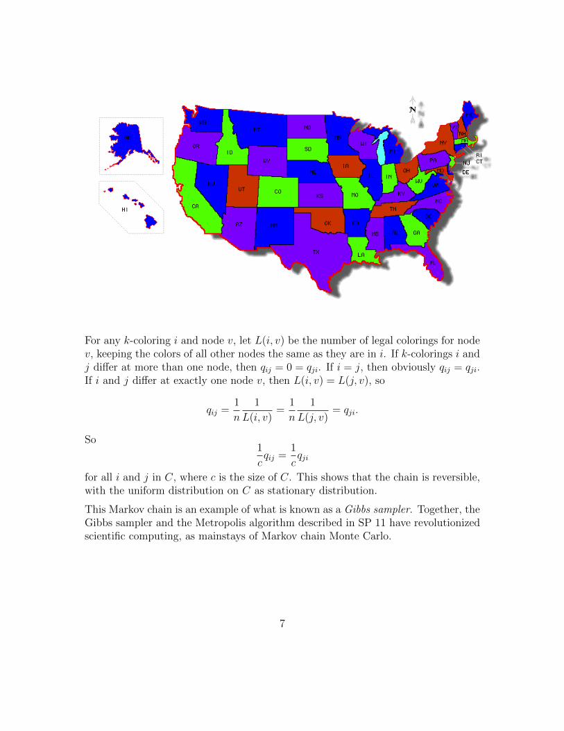
7. Let G be a network (also called a graph); there are n nodes, and for each pair ofdistinct nodes, there either is or isn’t an edge joining them. We have a set of k colors,e.g., if k = 7 the color set may be {red, orange, yellow, green, blue, indigo, violet}.A k-coloring of the network is an assignment of a color to each node, such that twonodes joined by an edge can’t be the same color. For example, a 4-coloring of the 50states in the U.S. is shown below (created using http://monarch.tamu.edu/⇠maps2/),where the corresponding network has 50 nodes (one for each state), with an edge be-tween two di↵erent states if and only if they share a border of nonzero length. Graphcoloring is an important topic in computer science, with wide-ranging applicationssuch as coloring a map, scheduling tasks, and in the game of Sudoku.
Suppose that it is possible to k-color G. Form a Markov chain on the space of allk-colorings of G, with transitions as follows: starting with a k-coloring of G, pick auniformly random node, figure out what the legal colors are for that node, and thenrepaint that node with a uniformly random legal color (note that this random colormay be the same as the current color). Show that this Markov chain is reversible,and find its stationary distribution.
Let C be the set of all k-colorings of G, and let qij
be the transition probability ofgoing from i to j for any k-colorings i and j in C. We will show that q
ij
= q
ji
, whichimplies that the stationary distribution is uniform on C.
6
For any k-coloring i and node v, let L(i, v) be the number of legal colorings for nodev, keeping the colors of all other nodes the same as they are in i. If k-colorings i andj di↵er at more than one node, then q
ij
= 0 = q
ji
. If i = j, then obviously q
ij
= q
ji
.If i and j di↵er at exactly one node v, then L(i, v) = L(j, v), so
q
ij
=1
n
1
L(i, v)=
1
n
1
L(j, v)= q
ji
.
So1
c
q
ij
=1
c
q
ji
for all i and j in C, where c is the size of C. This shows that the chain is reversible,with the uniform distribution on C as stationary distribution.
This Markov chain is an example of what is known as a Gibbs sampler. Together, theGibbs sampler and the Metropolis algorithm described in SP 11 have revolutionizedscientific computing, as mainstays of Markov chain Monte Carlo.
7