DI

SC

US

SI

ON

P

AP

ER

S

ER

IE

S

Forschungsinstitut zur Zukunft der ArbeitInstitute for the Study of Labor

Star Wars: The Empirics Strike Back

IZA DP No. 7268

March 2013

Abel BrodeurMathias LéMarc SangnierYanos Zylberberg

Star Wars: The Empirics Strike Back

Abel Brodeur Paris School of Economics,

CEP, London School of Economics and IZA

Mathias Lé Paris School of Economics

Marc Sangnier

Aix-Marseille University, CNRS and EHESS

Yanos Zylberberg

CREI, Universitat Pompeu Fabra

Discussion Paper No. 7268 March 2013

IZA

P.O. Box 7240 53072 Bonn

Germany

Phone: +49-228-3894-0 Fax: +49-228-3894-180

E-mail: iza@iza.org

Any opinions expressed here are those of the author(s) and not those of IZA. Research published in this series may include views on policy, but the institute itself takes no institutional policy positions. The IZA research network is committed to the IZA Guiding Principles of Research Integrity. The Institute for the Study of Labor (IZA) in Bonn is a local and virtual international research center and a place of communication between science, politics and business. IZA is an independent nonprofit organization supported by Deutsche Post Foundation. The center is associated with the University of Bonn and offers a stimulating research environment through its international network, workshops and conferences, data service, project support, research visits and doctoral program. IZA engages in (i) original and internationally competitive research in all fields of labor economics, (ii) development of policy concepts, and (iii) dissemination of research results and concepts to the interested public. IZA Discussion Papers often represent preliminary work and are circulated to encourage discussion. Citation of such a paper should account for its provisional character. A revised version may be available directly from the author.

IZA Discussion Paper No. 7268 March 2013

ABSTRACT

Star Wars: The Empirics Strike Back* Journals favor rejection of the null hypothesis. This selection upon tests may distort the behavior of researchers. Using 50,000 tests published between 2005 and 2011 in the AER, JPE, and QJE, we identify a residual in the distribution of tests that cannot be explained by selection. The distribution of p-values exhibits a camel shape with abundant p-values above 0.25, a valley between 0.25 and 0.10 and a bump slightly below 0.05. The missing tests (with p-values between 0.25 and 0.10) can be retrieved just after the 0.05 threshold and represent 10% to 20% of marginally rejected tests. Our interpretation is that researchers might be tempted to inflate the value of those almost-rejected tests by choosing a “significant” specification. We propose a method to measure inflation and decompose it along articles’ and authors’ characteristics. JEL Classification: A11, B41, C13, C44 Keywords: hypothesis testing, distorting incentives, selection bias, research in economics Corresponding author: Yanos Zylberberg CREI, Universitat Pompeu Fabra Ramon Trias Fargas, 25-27 08005 Barcelona Spain E-mail: yzylberberg@crei.cat

* We thank Orley Ashenfelter, Regis Barnichon, Marianne Bertrand, Thomas Breda, Paula Bustos, Colin Camerer, Andrew Clark, Gabrielle Fack, Patricia Funk, Jordi Gali, Nicola Gennaioli, Alan Gerber, Penny Glodberg, Libertad González, David Hendry, Emeric Henry, Lawrence Katz, James MacKinnon, Steve Pischke, Thijs van Rens, Tom Stanley, Harald Uhlig, Rainer Winkelmann and seminar participants at AMSE, CREI, EEA Meetings and Universitat Pompeu Fabra for very useful remarks and encouragements. Financial support from the Fonds Québécois de la Recherche sur la Société et la Culture, from Region Île-de-France, and from the European Research Council under the European Union’s Seventh Framework Programme (FP7/2007-2013) / ERC Grant agreement n° 241114 is gratefully acknowledged by Abel Brodeur, Mathias Lé, and Yanos Zylberberg.

If the stars were mine

I’d give them all to you

I’d pluck them down right from the sky

And leave it only blue.

“If The Stars Were Mine” by Melody Gardot

1 Introduction

The introduction of norms–confidence at 95% or 90%–and the use of eye-catchers–

stars–have led the academic community to accept more easily starry stories with

marginally significant coefficients than starless ones with marginally insignificant

coefficients.1 As highlighted by Sterling (1959), this effect has modified the selec-

tion of papers published in journals and arguably biased publications toward tests

rejecting the null hypothesis. This selection is not unreasonable. The choice of a

norm was precisely made to strongly discriminate between rejected and accepted

hypotheses.

As an unintended consequence, researchers may now anticipate this selection and

consider that it is a stumbling block for their ideas to be considered. As such, among

a set of acceptable specifications for a test, they may be tempted to keep those with

the highest statistics in order to increase their chances of being published. Keeping

only such specifications would lead to inflation in the statistics of observed tests.

Inflation and selection are different. Selection (rejection or self-censorship) con-

sists in the non-publication of the paper given the specification displayed. Inflation is

a publication-oriented choice of the displayed specification among the set of accept-

able specifications. The choice of the right specification may depend on its capacity

to detect an effect.2

In our interpretation, inflation can be distinguished from selection as the for-

mer should have different empirical implications than the latter. We assume that

selection results in a probability of being published that increases with the value of

test statistics presented in a paper. Inflation would not necessarily satisfy this prop-

erty. Imagine that there are three types of results, green lights are clearly rejected

tests, red lights clearly accepted tests and amber lights uncertain tests, i.e. close

1Fisher (1925) institutionalized the significance levels. R. A. Fisher supposedly decided toestablish the 5% level since he was earning 5% of royalties for his publications. It is howevernoticeable that, in economics, the academic community has converged toward 10% as being thefirst hurdle to pass, maybe because of the stringency of the 5% one.

2Authors may be tempted to shake their data before submitting a paper, or stop exploringfurther specifications when finding a “significant” one. Bastardi et al. (2011) and Nosek et al.(2012) explicitly refer to this wishful thinking in data exploration.

2

to the 5% or 10% statistical significance thresholds but not there yet. We argue

that researchers would mainly inflate when confronted with an amber test such as

to paint it green, rather than in the initially red and green cases where inflation

does not change the status of a test. In other words, we should expect a shortage of

amber tests relatively to red and green ones. The shift in the observed distribution

of statistics would be inconsistent with the previous assumption on selection. There

would be (i) a valley (not enough tests around 0.15 as if they were disliked relatively

to 0.30 tests) and (ii) the echoing bump (too many tests slightly under 0.05 as if

they were preferred to 0.001 tests).

We find evidence for this pattern. The distribution of tests statistics published in

three of the most prestigious economic journals over the period 2005-2011 exhibits

a sizable under-representation of marginally insignificant statistics. In a nutshell,

once tests are normalized as z-statistics, the distribution has a camel shape with (i)

missing z-statistics between 1.2 and 1.65 (p-values between 0.25 and 0.10) and a local

minimum around 1.5 (p-value of 0.12), (ii) a bump between 2 and 4 (p-values slightly

below 0.05). We argue that this pattern cannot be explained by selection and derive

a lower bound for the inflation bias under the assumption that selection should be

weakly increasing in the exhibited z-statistics. We find that ten to twenty percent

of tests with p-values between 0.05 and 0.0001 are misallocated. Interestingly, the

interval between the valley and the bulk of p-values corresponds precisely to the

highest marginal returns for the selection function.3

To our knowledge, this project is the first to identify a pattern of published tests

that cannot be explained by selection and to propose a way to measure it.4 To achieve

this, we conducted a census of tests in the literature. Identifying tests necessitates

a good understanding of the argument developed in an article and a strict process

avoiding any subjective selection of tests. This collecting process generated 50, 078

tests grouped in 3, 389 tables (or results subsections) and 641 articles published in

the American Economic Review, the Journal of Political Economy, and the Quarterly

Journal of Economics between 2005 and 2011.

3It is theoretically difficult to separate the estimation of inflation from selection: one mayinterpret selection and inflation as the equilibrium outcome of a game played by editors/refereesand authors as in the model of Henry (2009). Editors and referees prefer to publish results that are“significant”. Authors are tempted to inflate (with a cost), which pushes editors toward being evenmore conservative and exacerbates selection and inflation. A strong empirical argument in favor ofthis game between editors/referees and authors would be an increasing selection even below 0.05,i.e. editors challenge the credibility of rejected tests. Our findings do not seem to support thispattern.

4Gadbury and Allison (2012) recently proposed a method which analyzes the distribution oftests very close to the statistical significance thresholds and compares amber-red tests with amber-green tests. Their analysis is developed in the same spirit as ours, but is local and has not beenimplemented.

3

In addition to the census of tests, we collect a broad range of information on each

paper and author. This allows us to compare the distribution of published tests along

various dimensions. For example, we find evidence that inflation is less present in

articles where stars are not used as eye-catchers. To make a parallel with central

banks, the choice not to use eye-catchers might be considered as a commitment to

keep inflation low.5 Inflation is also smaller in articles with theoretical models, or

in articles using data from randomized control trials or laboratory experiments. We

also present evidence that papers published by tenured and older researchers are less

prone to inflation.

The literature on tests in economics was flourishing in the eighties and already

shown the importance of selection and the possible influence of inflation. On in-

flation, Leamer and Leonard (1983) and Leamer (1985) point out the fact that

inferences drawn from coefficients estimated in linear regressions are very sensitive

to the underlying econometric model. They suggest to display the range of infer-

ences generated by a set of models. Leamer (1983) rules out the myth inherited

from the physical sciences that econometric inferences are independent of priors: it

is possible to exhibit both a positive and a negative effect of capital punishment on

crime depending on priors on the acceptable specification. Lovell (1983) and Denton

(1985) study the implications of individual and collective data mining. In psycho-

logical science, the issue has also been recognized as a relatively common problem

(see Simmons and Simonsohn 2011 and Bastardi et al. 2011).

On selection, the literature has referred to the file drawer problem: statistics

with low values are censored by journals. We consider this as being part of selection

among other mechanisms such as self-censoring of insignificant results by authors.

A large number of recent publications quantify the extent to which selection distorts

published results (see Ashenfelter and Greenstone 2004 or Begg and Mazumdar

1994). Ashenfelter et al. (1999) propose a meta-analysis of the Mincer equation

showing a selection bias in favor of significant and positive returns to education. A

generalized method to identify reporting bias has been developed by Hedges (1992)

and extended by Doucouliagos and Stanley (2011). Card and Krueger (1995) and

Doucouliagos et al. (2011) are two other examples of meta-analysis dealing with

publication bias. The selection issue has also received a great deal of attention in

the medical literature (Berlin et al. 1989, Ioannidis 2005, Ridley et al. 2007), in

psychological science (Simmons and Simonsohn 2011, Fanelli 2010a) or in political

science (Gerber et al. 2010).

5However, such a causal interpretation might be challenged: researchers may give up on starsprecisely when their use is less relevant, either because coefficients are very significant and the testof nullity is not a particular concern or because coefficients are not significant.

4

Section 2 details the methodology to construct the dataset and provides some

information on tests’ meta-data. Section 3 documents the distribution of tests.

Section 4 proposes a method to measure inflation. Finally, we discuss the main

results and present the sub-samples’ analysis in section 5.

2 Data

In this section, we describe the reporting process of tests published in the American

Economic Review, the Journal of Political Economy, and the Quarterly Journal of

Economics between 2005 and 2011. We then provide some descriptive statistics.

2.1 Reporting process

The ideal measure of interest of this article is the reported value of formal tests of

central hypotheses. In practice, the large majority of those formal tests are two-

sided tests for regressions’ coefficients and are implicitly discussed in the body of

the article (i.e. “coefficients are significant”).6 To simplify the exposition we explain

the process as if we only had two-sided tests for regressions’ coefficients but the

description applies to our treatment of other tests.

Not all coefficients reported in tables should be considered as tests of central

hypotheses. Accordingly, we trust the authors and report tests that are discussed

in the body of the article except if they are explicitly described as controls. The

choice of this process helps to get rid of cognitive bias at the expense of parsimony.

With this mechanical way of collecting tests we also report statistical tests that the

authors may expect to fail, but we do not report explicit placebo tests. When the

status of a test was unclear when reading the paper, we prefer to add a non-relevant

test than censor a relevant one.

As we are only interested in tests of central hypotheses of articles, we also exclude

descriptive statistics or groups comparisons.7 A specific rule concerns two-stage

procedures. We do not report first-stages, except if the first-stage is described by

authors as a major contribution of the article. We do include tests in extensions or

robustness tests and report numbers exactly as they are presented in articles, i.e.

we never round them up or down.

We report some additional information on each test, i.e. the issue of the journal,

685% of collected test are presented using a regressions’ coefficient and their associated standarderrors.

7A notable exception to this rule was made for experimental papers where results are sometimespresented as mean comparisons across groups.

5

the starting page of the article and the position of the test in the article, its type

(one-sided, two-sided, correlation test, etc.) and the status of the test in the article

(main, non-main). We prefer to be conservative and only attribute the status of“non-

main” statistics if evidence are clearly presented as “complementary”, “additional” or

“robustness checks”. Finally, the number of authors, JEL codes when available, the

presence of a theoretical model, the type of data (laboratory experiment, randomized

control trials or other), the use of eye-catchers (stars or other formatting tricks such

as bold printing), the number of research assistants and researchers the authors wish

to thank, the rate of tenure among authors and data and code availability on the

website of the journal are also recorded. We do not report the sample size and

the number of variables (regressors) as this information is not always provided by

authors. Exhaustive reporting rules we used are presented in the online appendix.

We also collected information from curricula vitae of all the authors who pub-

lished in the three journals over the period of interest. We gathered information

about academic affiliation at the time of the publication, the position at the main

institution (assistant professor, associate professor, etc.), whether the author is or

was an editor (or a member of an editorial board) of an economic journal, and the

year and the institution where the PhD was earned.

2.2 Descriptive statistics

The reporting process described above provides 50, 078 tests. Journals do not con-

tribute equally: most of the tests come from the American Economic Review, closely

followed by the Quarterly Journal of Economics. The Journal of Political Economy

provides a little less than a fifth of the sample. Out of the 50, 078 tests extracted

from the three journals, around 30, 000 are rejected at the 10% significance level,

27, 000 at 5%, and 21, 000 at 1%.

Table 1 gives the decomposition of tests along several dimensions. The average

number of tests per article equals 78. It is surprisingly high but it is mainly driven by

some articles with a very large number of tests reported. The median article reports

58 tests and 5 tables. These figures are reasonable as tests are usually diluted

in many different empirical specifications. Imagine a paper with two variables of

interest (e.g. democracy and institutions), six different specifications per table and

five tables. We would report 60 coefficients, a bit more than our median article.

More than half of the articles use eye-catchers defined as the presence of stars

or bold printing in a table, excluding the explicit display of p-values. These starry

tests represent more than sixty percent of the total number of tests(the average

number of tests is higher in articles using eye-catchers). With the conservative way

6

of reporting main results, more than seventy percent of tables from which tests are

extracted are considered as main. More than a third of the articles in our sample

explicitly rely on a theoretical framework but when they do so, the number of tests

provided is not particularly smaller than when they do not. Only a fifth of articles

are single-authored.8

Tests using data from laboratory experiments or randomized control trials con-

stitute a small part of the overall sample. To be more precise, the AER publishes

relatively more experimental articles while the QJE seems to favor randomized con-

trolled trials. The overall contribution of both types is equivalent (with twice as

many laboratory experiments than randomized experiments but more tests in the

latter than in the former).

3 The distribution of tests

In this section, we describe the raw distribution of tests and propose methods to

alleviate the over-representation of round values and the potential overweight at-

tributed to articles with many tests. We then derive the distribution of tests and

comment on it.

The collecting process groups three types of measures : p-values, tests statistics

when directly reported by authors, and coefficients and standard errors for the vast

majority of tests. In order to get a homogeneous sample, we transform p-values into

the equivalent z-statistics (a p-value of 0.05 becomes 1.96). For tests reported using

coefficients and standard errors, we simply construct the ratio of the two.9 Recall

that the distribution of a t-statistic depends on the degrees of freedom, while that of a

z-statistic is standard normal. As we are unable to reconstruct the degrees of freedom

for all tests, we will treat these ratios as if they were following an asymptotically

standard normal distribution under the null hypothesis. Consequently, when the

sample size is small, the level of rejection we use is not adequate. For instance, some

tests for which we associate a z-statistic of z = 1.97 might not be rejected at the 5%

significance threshold.

The transformation into z-statistic allows us to observe more easily the fat tail of

tests (with small p-values). Figure 1(a) presents the raw distribution. Remark that

a very large number of p-values end up below the 0.05 significance threshold (more

8See Card and DellaVigna (2012, 2013) for recent studies about top journals in economics.9These transformations allow us to obtain direct or reconstructed statistics for all but three

types of tests collected: (i) tests reported as a zero p-value, (ii) tests reported as a p-value lowerthan a threshold (e.g. p < 0.001), and (iii) tests reported with a zero standard error. These threecases represent 727 tests, i.e. 1.45% of the total sample.

7

than 50% of tests are rejected at this significance level).

Two potential issues may be raised with the way authors report the value of their

tests and the way we reconstruct the underlying statistics. First, a small proportion

of coefficients and standard errors are reported with a pretty poor precision (0.020

and 0.010 for example). Reconstructed z-statistics are thus over-abundant for frac-

tions of integers (11,21,31,13,12,. . . ). Second, some authors report a lot of versions of

the same test. In some articles, more than 100 values are reported against 4 or 5

in others. Which weights are we suppose to give to the former and the latter in

the final distribution? This issue might be of particular concern as authors might

choose the number of tests they report depending on how close or far they are from

the thresholds.10

To alleviate the first issue, we randomly redraw a value in the interval of poten-

tial z-statistics given the reported values and their precision. In the example given

above, the interval would be [0.01950.0105

, 0.02050.0095

] ≈ [1.86, 2.16]. We draw a z-statistic from

a uniform distribution over the interval and replace the previous one. This reallo-

cation should not have any impact on the analysis other than smoothing potential

discontinuities in histograms.11

To alleviate the second issue, we construct two different sets of weights, account-

ing for the number of tests per article and per table in each article. For the first set

of weights, we associate to each test the inverse of the number of tests presented in

the same article such that each article contributes the same to the distribution. For

the second set of weights, we associate the inverse of the number of tests presented

in the same table (or result sub-section) multiplied by the inverse of the number of

tables in the article such that each article contributes the same to the distribution

and tables of a same article have equal weights.

Figure 1(b) presents the de-rounded distribution.12 The shape is striking. The

distribution presents a camel pattern with a local minimum around z = 1.5 (p-value

of 0.12) and a local maximum around 2 (p-value under 0.05). The presence of a

local maximum around 2 is not very surprising, the existence of a valley before more

so. Intuitively, selection could explain an increasing pattern for the distribution of

z-statistics at the beginning of the interval [0,∞). On the other hand, it is likely

10For example, one might conjecture that authors report more tests when the significance ofthose is shaky. Conversely, one may also choose to display a small number of satisfying tests asothers tests would fail.

11For statistics close to significance levels, we could have taken advantage of the informationembedded in the presence of a star. However, this approach could only have been implemented fora very reduced number of observations and only in cases where stars are used.

12In what follows, we use the word “de-rounded” to refer to statistics to which we applied themethod described above.

8

that there is a natural decreasing pattern of the distribution over the whole interval.

Both effects put together could explain the presence of a unique local maximum, a

local minimum before, less so. Our empirical strategy will consist in formalizing this

argument: only a shift of statistics can generate such a pattern and the inflation

bias seems to explain this shift.13

Figures 1(c) and (d) present the weighted distributions of de-rounded statistics.

The camel shape is more pronounced than for the unweighted distributions. A simple

explanation is that weighted distributions underweight articles and tables for which

a lot of tests are reported. For these articles and tables, our conservative way to

report tests might have included tests of non-central hypotheses.

The pattern shown in figures 1(b), (c) and (d) is very consistent. It is not driven

by a particular journal or a particular year. The last three sub-figures of figure 9

show the distributions for each of the three journals. The shape is also similar for

each specific year.

In figures 5 to 9, we plot the distribution of tests over sub-samples along some

characteristics of tests or articles. We analyze further the variations of inflation

across sub-samples in section 5, but we can already notice that the shape of the

distribution varies along several dimensions. For example, the camel shape is less

pronounced in articles without eye-catchers and articles with a theoretical contri-

bution (see figure 5). Similarly, inflation seems lower in papers written by senior

researchers whether seniority is captured by years since PhD, tenure or editorial

responsibilities (see figure 6). Inflation seems larger in articles that thank research

assistants (see figure 7). In contrast, it does not vary along data and codes availabil-

ity on journals’ website (see figure 8). Finally, inflation appears to be less intense in

articles using randomized control trials or laboratory experiments data (see figure

9). All in all, the pattern that we document is not invariant along authors’ and

articles’ characteristics.

13In the online appendix, we also test for discontinuities. We find evidence that the total distri-bution of tests presents a small discontinuity around the 0.10 significance threshold, but not mucharound the 0.05 or the 0.01 thresholds. This modest effect might be explained by the dilution ofhypothesis tested in journal articles. In the absence of a single test, empirical economists providemany converging arguments under the form of different specifications for a single effect. Besides, anempirical article is often dedicated to the identification of more than one mechanism. As such, thereal statistic related to an article is a distribution or a set of arguments and this dilution smoothespotential discrepancies around thresholds. The online appendix also presents an analysis using theBenford’s law to look for manipulation in reported coefficients and standard errors.

9

4 A method to measure inflation

In this section, we present a method to obtain an estimate of inflation. The basic

question this method attempts to answer is as follows: how much of the misalloca-

tion of test statistics can be attributed to inflation? The idea is that the observed

distribution of published z-statistics may be thought as generated by (i) an input

distribution, (ii) a selection over results, and (iii) a noise, which will partly capture

inflation. We first describe a very simple model of selection in academic publishing.

Then, we discuss the identification strategy and the different counterfactual distri-

butions to which we can compare the observed one. In our framework, under the

restricting assumption that selection favors high over low statistics, the ratio of the

observed density over the input density would be increasing in the exhibited statis-

tic. The empirical strategy will consist in capturing any violation of this prediction

and relating it to the inflation bias. We also discuss stories that may challenge this

interpretation. Finally, we apply this method to the distribution of tests presented

in the previous section.

4.1 The selection process

We consider a very simple theoretical framework of selection into journals. We

abstract from authors and directly consider the universe of working papers.14 Each

economic working paper has a unique hypothesis which is tested with a unique

specification. Denote z the absolute value of the statistic associated to this test and

ϕ the density of its distribution over the universe of working papers, the input.

A unique journal gives a value f(z, ε) to each working paper where ε is a noise

entering into the selection process.15 Working papers are accepted for publication

as long as they pass a certain threshold F , i.e. f(z, ε) ≥ F . Suppose without loss of

generality that f is strictly increasing in ε, such that a high ε corresponds to articles

with higher likelihood to be published, for a same z. Denote Gz the distribution of

ε conditional on the value of z.

The density of tests in journals (the output) can be written as:

ψ(z) =

∫∞0

[1f(z,ε)≥FdGz(ε)dε

]ϕ(z)∫∞

0

∫∞0

[1f(z,ε)≥FdGz(ε)dε

]ϕ(z)dz

.

14Note that the selection of potential economic issues into a working paper is not modeled here.You can think alternatively that this is the universe of potential ideas and selection would theninclude the process from the “choice” of idea to publication.

15We label here ε as a noise but it also captures inclinations of journals for certain articles, theimportance of the question, the originality of the methodology, or the quality of the paper.

10

The observed density of tests for a given z depends on the quantity of articles

with ε sufficiently high to pass the threshold and on the input. In the black box

which generates the output from the input, two effects intervene. First, as the value

of z changes, the minimum noise ε required to pass the threshold changes: it is

easier to get in, this is the selection effect. Second, the distribution Gz of this ε

might change conditionally on z. The quality of articles may differ along z: this

will be in the residual. We argue that this residual captures–among other potential

mechanisms–local shifts in the distribution. An inflation bias corresponds to such a

shift. In this framework, this would translate into productions of low ε just below

the threshold against very high ε above.

4.2 Identification strategy

Our empirical strategy consists in estimating how well selection might explain the

observed pattern and we interpret the residual as capturing inflation. This strategy

is conservative as it may attribute to selection some patterns due to inflation.

Let us assume that we know the distribution ϕ. The ratio of the output density

to the input density can be written as:

ψ(z)/ϕ(z) =

∫∞0

[1f(z,ε)≥FdGz(ε)dε

]∫∞0

∫∞0

[1f(z,ε)≥FdGz(ε)dε

]ϕ(z)dz

.

In this framework, once normalized by the input, the output is a function of the

selection function f and the conditional distribution of noise Gz. We will isolate

selection z 7→ 1f(z,ε) from noise Gz(ε) thanks to the following assumption.

Assumption 1 (Journals like stars). The function f is (weakly) increasing in z.

For a same noisy component ε, journals prefer higher z. Everything else equal,

a 10% test is not strictly preferred to a 9% one.

This assumption that journals, referees and authors prefer tests rejecting the

null may not be viable for high z-statistics. Such results could indicate an empirical

misspecification to referees. This effect, if present, should only appear for very large

statistics. Another concern is that journals may also appreciate clear acceptance of

the null hypothesis, in which case the selection function would be initially decreasing.

Journals and authors may privilege p-values very close to 1 and very close to 0, which

would fit the camel pattern with two bumps.16 We discuss the potential mechanisms

challenging this assumption at the end of this section.

16There is no way to formally reject this interpretation. However, we think that this effect ismarginal as the number of articles for which the central hypothesis is accepted is very small in oursample.

11

The identification strategy relies on two results. First, if we shut down any other

channel than selection (the noise is independent of z), we should see an increasing

pattern in the selection process, i.e. the proportion of articles selected ψ(z)/ϕ(z)

should be (weakly) increasing in z. We cannot explain stagnation or slowdowns in

this ratio with selection or self-censoring alone. Second and this is the purpose of

the lemma below, the reciprocal is also true: any increasing pattern for the ratio

output/input can be explained by selection alone, i.e. with a distribution of noise

invariant in z. Given any selection process f verifying assumption 1, any increasing

function of z (in a reasonable interval) for the ratio of densities can be generated

by f and a certain distribution of noise invariant in z. Intuitively, there is no way

to identify an inflation effect with an increasing ratio of densities, as an invariant

distribution of noise can always be considered to fit the pattern.

Lemma 1 (Duality). Given a selection function f , any increasing function g :

[0, Tlim] 7→ [0, 1] can be represented by a cumulative distribution of quality ε ∼ G̃,

where G̃ is invariant in z:

∀t, g(z) =

∫ ∞0

[1f(z,ε)≥FdG̃(ε)dε

]G̃ is uniquely defined on the subsample {ε,∃z ∈ [0,∞), f(z, ε) = F}, i.e. on the

values of noise for which some articles may be rejected (with insignificant tests) and

some others accepted (with significant tests).

Proof. In the appendix.

Following this lemma, the empirical strategy will consist in the estimation of the

best-fitting increasing function f̃ for the ratio ψ(z)/ϕ(z). We will find the weakly

increasing f̃ that minimizes the weighted distance with the ratio ψ(z)/ϕ(z):

∑i

[ψ(zi)/ϕ(zi)− f̃(zi)

]2

ϕ(zi),

where i is a test’s identifier.

In order to estimate our effects, we have focused on the ratio ψ(z)/ϕ(z). The

following corollary transforms the estimated ratio in a cumulative distribution of

z-statistics and relates the residual of the previous estimation to the number of

statistics unexplained by selection.

Corollary 1 (Residual). Following the previous lemma, there exists a cumulative

distribution G̃ which represents f̃ uniquely defined on {ε, ∃z ∈ [0, Tlim], f(z, ε) = F},

12

such that:

∀t, f̃(z) =

∫∞0

[1f(z,ε)≥FdG̃(ε)dε

]∫∞

0

∫∞0

[1f(z,ε)≥FdGz(ε)dε

]ϕ(z)dz

.

The residual of the previous estimation can be written as the difference between G̃

and the true Gz:

u(z) =G̃(h(z))−Gz(h(z))∫∞

0

∫∞0

[1f(z,ε)≥FdGz(ε)dε

]ϕ(z)dz

,

where h is defined as f(z, ε) ≥ F ⇔ ε ≥ h(z). Define ψ̃(z) = (1− G̃(h(z)))ϕ(z) the

density of z-statistics associated to G̃, then the cumulated residual is simply∫ z

0

u(τ)ϕ(τ)dτ =

∫ z

0

ψ(τ)dτ −∫ z

0

ψ̃(τ)dτ.

Proof. In the appendix.

This corollary allows us to map the cumulated residual of the estimation with

a quantity that can be interpreted. Indeed, given z,∫ z

0ψ(τ)dτ −

∫ z0ψ̃(τ)dτ is the

number of z-statistics between [0, z] that cannot be explained by a selection function

verifying assumption 1.

4.3 Input

A difficulty arises in practice. The previous strategy can be implemented for any

given input distribution. But what do we want to consider as the exogenous input

and what do we want to include in the selection process? In the process that occurs

before publication, there are several choices that may change the distribution of

tests: the choice of the research question, the dataset, the decision to submit and

the acceptance of referees. We think that all these processes are very likely to satisfy

assumption 1 (at least for z-statistics not extremely high) and that the input can be

taken as the distribution before all these choices. All the choices (research question,

dataset, decision to create a working paper, submission and acceptance) will thus

be included in the endogenous process.

The idea here is to consider a large range of distributions for the input. The

classes of distribution should ideally include unimodal (with the mode being 0)

distribution as the distributions of some of our subsamples are unimodal in 0, and

ratio distributions as the vast majority of our tests are ratio tests. They should also

capture as much as possible of the fat tail of the observed distribution (distributions

13

should allow for the large number of rejected tests and very high z-statistics). Let

us consider three candidate classes.

Class 1 (Gaussian). The Gaussian/Student distribution class arises as the distri-

bution class under the null hypothesis of t-tests. Under the hypothesis that tests are

t-tests for independent random processes following normal distributions centered in

0, the underlying distribution is a standard normal distribution (if all tests are done

with infinite degrees of freedom), or a mix of Student distributions (in the case with

finite degrees of freedom).

This class of distributions naturally arises under the assumption that the underly-

ing hypotheses are always true. For instance, tests of correlations between variables

that are randomly chosen from a pool of uncorrelated processes would follow such

distributions. From the descriptive statistics, we know that selection should be quite

drastic when we consider a normal distribution for the exogenous input. The output

displays more than 50% of rejected tests against 5% for the normal distribution. A

normal distribution would rule out the existence of statistics around 10. In order to

account for the fat tail observed in the data, we extend the class of exogenous inputs

to Cauchy distributions. Remark that a ratio of two normal distributions follows a

Cauchy law. In that respect, the class of Cauchy distributions satisfies all the ad

hoc criteria that we wish to impose on the input.

Class 2 (Cauchy). The Cauchy distributions are fat-tail ratio distributions which

extend the Gaussian/Student distributions: (i) the standard Cauchy distribution co-

incides with the Student distribution with 1 degree of freedom, (ii) this distribution

class is, in addition, a strictly stable distribution.

Cauchy distributions account for the fact that researchers identify mechanisms

among a set of correlated processes, for which the null hypothesis might be false. As

such, Cauchy distribution allows us to extend the input to fat-tail distributions.

The last approach consists in an empirical counterfactual distribution of statistics

obtained by performing random tests on large and classic datasets.

Class 3 (Empirical). We randomly draw 4 variables from the World Development

Indicators (WDI) and run 2, 000, 000 regressions between these variables and stock

the z-statistic behind the first variable.17 Other datasets/sample can be considered

and the shapes are very close.

17To be consistent with the literature, we just ran two million regressions (see Sala-i Martin 1997and Hendry and Krolzig 2004).

14

How do these different classes of distributions compare to the observed distribu-

tion of published tests?

Figures 2(a) and (b) show how poorly the normal distribution fits the observed

one. The assumption that input comes from uncorrelated processes can only be rec-

onciled with the observed output through a drastic selection (which would generate

the observed fat tail from a Gaussian tail). The fit is slightly better for the standard

Cauchy distribution, e.g. the Student distribution of degree 1. The proportion of

rejected tests is then much higher with 44% of rejected tests at the 0.05 significance

level and 35% at 0.01. Cauchy distributions centered in 0 and the empirical coun-

terfactuals of statistics from the World Development Indicators have fairly similar

shapes. Figures 2(c) and (d) show that the Cauchy distributions as well as the WDI

empirical input may help to capture the fat tail of the observed distribution. Figures

2(e) and (f) focus on the tail: Cauchy distributions with parameters between 0.5 and

2 as well as the empirical placebo fit very well the tail of the observed distribution.

More than the levels of the densities, it is their evolution which gives support to

the use of these distributions as input: if we suppose that there is no selection nor

inflation once passed a certain threshold (p<0.000001 for these levels), we should

indeed observe a constant ratio output/input.

In what follows, we will first consider as exogenous inputs (i) the WDI empirical

input which will be the higher bound in terms of fat-tail (it is close to a Cauchy of

parameter 1.5); (ii) the Student distribution; (iii) and a rather thin-tail distribution,

i.e. the Cauchy distribution of parameter 0.5. These distributions cover a large

spectrum of shapes and results are not sensitive to changes in the choice of inputs.

As such, we will finally restrict the analysis to the empirical WDI input for the sake

of brevity.

4.4 Discussion

The quantity that we isolate is a cumulated residual (the difference between the

observed and the predicted cumulative function of z-statistics) that cannot be ex-

plained by selection. In our interpretation, it will capture a local shift of z-statistics

that reflects the inflation bias. In addition, this quantity is a lower bound of infla-

tion as any globally increasing pattern (in z) in the inflation mechanism would be

captured as part of the selection effect.

Several observations may challenge our interpretation. First, the noise ε actually

includes the quality of a paper and quality may be decreasing in z. The amount of

efforts put in a paper might end up being higher with very low p-values or p-values

around 0.15. Authors might for instance erroneously estimate selection by journals

15

and produce low effort in certain ranges of z-statistics. Second, the selection function

may not be increasing as a well-estimated zero might be interesting and there are no

formal tests to exclude this interpretation. We do not present strong evidence against

this mechanism. However, two observations make us confident that this preference

for well-estimated zero does not drive the whole camel shape. The first argument is

based on anecdotal evidence: very few papers of the sample present a well-estimated

zero as their central result. Second, this preference for well-estimated zero should not

depend on whether eye-catchers are used or whether a theoretical model is attached

to the empirical analysis and we find disparities along those characteristics. Similarly,

this preference should not depend on authors’ characteristics but inflation seems to

vary along these features.

In addition, imagine that authors could predict exactly where tests will end

up and decide to invest in the working paper accordingly. This ex ante selection

is captured by the selection term as long as it displays an increasing pattern, i.e.

projects with expected higher z-statistics are always more likely to be undertaken.

We may think of a very simple setting where it is unlikely to be the case: when

designing experiments (or randomized control trials), researchers compute power

tests such as to derive the minimum number of participants for which an effect can be

statistically captured. The reason is that experiments are expensive and costs need

to be minimized under the condition that a test may settle whether the hypothesis

can or cannot be rejected. We should expect a thinner tail for those experimental

settings and this is exactly what we observe. For this reason, we will not apply our

methodology to these samples. In the other cases, the limited capacity of authors to

predict where the z-statistics may end up as well as the modest incentives to limit

oneself to small samples make it more unlikely.

5 Results

In this section, we first apply our estimation strategy to the full sample and propose

non-parametric and parametric analyses. Then, we divide tests into sub-samples

and we provide the results separately for each sub-samples.

5.1 Non-parametric application

We group observed z-statistics by bandwidth of 0.01 and limit our study to the

interval [0, 10]. Accordingly, the analysis is made on 1, 000 bins. As the empirical

input appears in the denominator of the ratio ψ(z)/ϕ(z), we smooth it with an

16

Epanechnikov kernel function and a bandwidth of 0.1 in order to dilute noise (for

high z, the probability to see an empty bin is not negligible).

Figures 3(a) and (b) give both the best increasing fit for the ratio of observed

density to the empirical WDI input and the associated partial sum of residuals,

i.e. the lower bound for the inflation bias.18 Results are computed with the Pool-

Adjacent-Violators Algorithm.

Two interpretations emerge from this estimation. First, the best increasing fit

displays high marginal returns to the value of statistics ∂f̃(z)/∂z only for z ∈ [1.5, 2],

and a plateau thereafter. Selection is intense precisely where it is supposed to be

discriminatory, i.e. before the thresholds. Second, the misallocation of z-statistics

captured by the cumulated residuals starts to increase slightly before z = 2 up to 4

(the bulk between p-values of 0.05 and 0.0001 cannot be explained by an increasing

selection process alone). At the maximum, the misallocation reaches 0.025, which

means that 2.5% of the total number of t-statistics are misallocated between 0 and 4.

As there is no residual between 0 and 2, we compare this 2.5% to the total proportion

of z-statistics between 2 and 4, i.e. 30% of the total population. The conditional

probability of being misallocated for a z-statistic between 2 and 4 is thus around

8%. As shown by figures 3(c), (d), (e), (f), results do not change when the input

distribution is approximated by a Student distribution of degree 1 and a Cauchy

distribution of parameter 0.5. The results are very similar both in terms of shape

and magnitude.

A concern in this estimation strategy is that the misallocation could reflect dif-

ferent levels of quality between articles with z-statistics between 2 and 4 compared

to the rest. We cannot rule out this possibility. However, two observations gives

support to our interpretation: the start of the misallocation is right after (i) the first

significance thresholds, and (ii) the zone where the marginal returns of the selection

function are the highest.19

As already suggested by the shapes of weighted distributions (figures 1(c) and

(d)), the results are much stronger when the distribution of observed z-statistics is

corrected such that each article or each table contributes the same to the overall

distribution. Sub-figures 10(a)-(d) presented in the online appendix plot the best

increasing non-parametric fits against the empirical WDI input and associated cu-

mulated residuals when distributions are weighted by article or table. The shape

18Note that there are less and less z-statistics per bins of width 0.01. On the right-hand partof the figure, we can see lines that look like raindrops on a windshield. Those lines are bins forwhich there is the same number of observed z-statistics. As this observed number of z-statistics isdivided by a decreasing and continuous function, this gives these increasing patterns.

19This result is not surprising as it comes from the mere observation that the observed ratio ofdensities reaches a maximum between 2 and 4.

17

of misallocation is similar but the magnitude is approximately twice as large as in

the case without weights: the conditional probability of being misallocated for a

z-statistic between 2 and 4 is now between 15% and 20%. In a way, the weights may

compensate for our very conservative reporting process.

Even though the results are globally inconsistent with the presence of only se-

lection, the distribution of misallocated z-statistics is a bit surprising (and not com-

pletely consistent with inflation): the surplus observed between 2 and 4 is here

compensated by a deficit after 4. Inflation would predict such a deficit before 2 (be-

tween 1.2 and 1.7, which corresponds to the valley between the two bumps). This

result comes from the conservative hypothesis that the pattern observed in the ratio

of densities should be attributed to the selection function as long as it is increasing.

Accordingly, the stagnation of the ratio observed before 1.7 is captured by the selec-

tion function. Nonetheless, as the missing tests still fall in the bulk between 2 and

4, they allow us to identify a violation of the presence of selection alone: the bump

is too big to be reconciled with the tail of the distribution. In the next sub-section,

we get rid of this inconsistency by imposing more restricting assumptions on the

selection process.

5.2 Parametric application

A concern about the previous analysis is that it attributes the surplus of misallocated

tests between 2 and 4 to missing tests after this bulk. The mere observation of the

distribution of tests does not give the same impression. Apart from the bulk between

2 and 4, the other anomaly is the valley around z = 1.5. This valley is considered

as a stagnation of the selection function in the previous non-parametric case. We

consider here a less conservative test by estimating the selection function under the

assumption that it should belong to a set of parametric functions.

Assume now that the selection process can be approximated by an exponential

polynomial function, i.e. consider a selection function of the following form:

f(z) = c+ exp(a0 + a1z + a2z2).

The pattern of this function allows us to account for the concave pattern of the

observed ratio of densities.20

Figure 4 presents the best parametric fits and the partial sums of residuals. As in

the non-parametric case, the figure presents results using the empirical WDI input,

the Student input, and the Cauchy(0.05) input. Contrary to the non-parametric

20The analysis can be made with simple polynomial functions but it slightly worsens the fit.

18

case, the misallocation of t-statistics starts after z = 1 (p-values around 0.30) and is

decreasing up to z = 1.65 (p-values equals to 0.10 and first significance threshold).

These missing statistics are then completely retrieved between 1.65 and 3 − 4, and

no misallocation is left for the tail of the distribution. Remark that the magnitude

of misallocation is very similar to the non-parametric case. Sub-figures 11(a)-(d)

presented in the online appendix plot the best increasing parametric fits against

the empirical WDI input and associated cumulated residuals when distributions are

weighted by article or table.

5.3 Subsample analysis

Information we collected about articles and authors allow us to split the full sample

of tests into sub-samples along various dimensions and to compare our measure of

inflation across sub-samples. It seems reasonable to expect inflation to vary along

characteristics of the paper, e.g. the importance of the empirical contribution, or

characteristics of the authors, e.g. the expected returns from a publication in a

prestigious journal.21

In this sub-section, we split the full sample of published z-statistics along various

dimensions and present associated distributions. We perform a different estimation

of the best-fitting selection function on each subsample using the method presented

above. For space consideration, we restrict ourselves to the analysis of unweighted

distributions. Figures of corresponding cumulated residuals from parametric and

non-parametric estimations using the empirical WDI input are presented in the

online appendix and summarized in table 2.

In sub-samples presented in figure 5, we split the full sample depending on the

presentation of the results and the content of the paper. Sub-figures (a) and (b)

distinguish between tests presented using eye-catchers or not. The analysis on the

eye-catchers sample shows that misallocated z-statistics between 0 and 4 account

for more than 3% of the total number of tests against 1% for the no eye-catchers

sample. The conditional probability of being misallocated for a z-statistic between

2 and 4 is around 12% in the eye-catchers sample against 4% in the no eye-catchers

one. Not using stars may act as a commitment for researchers to not be influenced

by the distance of their tests from the 10% or 5% significance thresholds. Sub-figures

(c) and (d) split the sample depending on whether the test is presented as a main

21However, this analysis cannot be considered as causal. From the blank page to the publishedresearch article, researchers choose the topic, collect data, decide on co-authorship, where to submitthe paper, etc. All these choices are made either simultaneously or sequentially. None of them canbe considered as exogenous since they are related to the expected quality of the outcome and toits expected likelihood to be accepted for publication.

19

test or not (tests or results explicitly presented as “complementary”, “additional” or

“robustness checks”). The camel shape is more pronounced for results not presented

as a main result. The emphasis put on the empirical analysis may also depend on

the presence of a theoretical contribution. In articles having a theoretical content,

the main contribution of the paper is divided between theory and empirics. This

intuition may explain the results shown in sub-figures (e) and (f): there seems to be

almost no inflation in articles with a theoretical model.

One might consider that articles and ideas from researchers with higher academic

rankings are more likely to be valued by editors and referees. Accordingly, inflation

may vary with authors’ status : well-established researchers facing less intense se-

lection should have less incentives to inflate. A first proxy that we use to capture

authors’ status is experience. Sub-figures (a) and (b) of figure 6 present the distribu-

tions of tests in articles having an average PhD-age of authors below and above the

median PhD-age of the sample. We find that inflation is more pronounced among

relatively younger authors. A second indicator reflecting authors’ status is whether

they are involved in the academic editorial process. Sub-figures (c) and (d) split

the sample in two groups: the former is made of articles published by authors who

were not editors or members of editorial boards before publication, while the latter

is made of articles published by at least one editor or member of an editorial board.

Inflation appears to be slightly more intense among the first group. Another proxy

of authors’ status which is strongly related to incentives to publish in top journals

is whether authors are tenured or not. We compute the rate of tenure among au-

thors of each paper and split the sample along this dimension in sub-figures (e) and

(f).22 The first distribution is the one of tests from articles published by at least

one tenured author three years before publication. The second distribution of tests

comes from articles published by authors who were all non-tenured three years be-

fore publication. We find that the presence of at least one tenured researcher among

authors is associated with a strong decline in inflation. All in all, this finding seems

in line with the idea that inflation varies along expected returns to publication in

prestigious journals.

Sub-figures (a) and (b) of figure 7 split the sample of published tests between

single-authored and co-authored papers: inflation seems to be larger in single-

authored papers. We also collected the number of individuals the authors thank

22Getting information about effective tenure status of authors may be difficult as positions’denomination varies across countries and institutions. Here, we only consider full professors astenured researchers. Besides, the length of the publication process makes it hard to know theprecise status of authors at the time of submission. Here, we arbitrarily consider positions ofauthors three years before publication.

20

in the published version of the paper. Sub-figures (c) and (d) split the sample be-

tween articles that use research assistants and those that do not. Sub-figures (e) and

(f) split the sample between articles with a number of thanks (excluding research

assistants) below or above the median. Inflation tends to be a bit smaller when

no research assistants are thanked and in articles with a relatively low number of

thanks.

In figure 8 we investigate whether data and programs disclosure for replica-

tion alters inflation. Whether data and codes are available on the website of the

journal for replication purposes has attracted a great deal of attention lately (see

Dewald et al. (1986) and McCullough et al. 2008). For instance, the AER imple-

mented a mandatory data and code archive few years ago. On the other hand, the

JPE archive access is available solely to JPE subscribers. We verify for each article

whether data and codes are available on the website of the journal. The analysis of

the different sub-samples does not show conclusive evidence that data or programs

availability mitigates inflation.

To conclude this sub-sample analysis, we investigate the distribution of tests

depending on the source of data. There is an increasing use of randomized control

trials in economics and many researchers advocate that it is a very useful way to

accumulate knowledge without relying on questionable theory or statistical methods.

In figure 9, sub-figure (a) presents the distribution of tests relying on data obtained

from randomized control trials. Sub-figure (b) plots the distribution of tests that rely

on data from laboratory experiments, and sub-figure (c) all other type of data. The

randomized control trials data distribution exhibits a very smooth pattern: there is

neither a valley between 0.25 and 0.10, nor a significant bump around 0.05. There is

small evidence of inflation for the sub-sample of laboratory experiments. However,

z-statistics seem to disappear after the 0.05 threshold in both cases. As argued

before, randomized control trials and laboratory experiments are designed such as

to minimize the costs while being able to detect an effect. Very large z-statistics are

thus less likely to appear which violates our hypothesis that selection is increasing.

Hence, we cannot evaluate the inflation bias for these two sub-samples with our

methodology.

Finally, we do not find clear evidence that inflation differs across journals as

illustrated by sub-figures (d), (e), and (f) of figure 9.

Overall, we find that the intensity of inflation varies along different dimensions of

papers’ and authors’ characteristics. Interestingly, these variations seem consistent

with the returns of displaying a “significant” empirical analysis.

21

6 Conclusion

He who is fixed to a star does not change his mind. (Da Vinci)

In this paper, we have identified a misallocation in the distribution of the test

statistics in some of the most respected academic journals in economics. Our analy-

sis suggests that the pattern of this misallocation is consistent with what we dubbed

an inflation bias : researchers might be tempted to inflate the value of those almost-

rejected tests by choosing a “significant” specification. We have also quantified this

inflation bias : among the tests that are marginally significant, 10% to 20% are

misreported. These figures are likely to be lower bounds of the true misallocation as

we use very conservative collecting and estimating processes. Results presented in

this paper may have potentially different implications for the academic community

than the already known publication bias. Even though it is unclear whether these

biases should be larger or smaller in other journals and disciplines,23 it raises ques-

tions about the importance given to values of tests per se and the consequences for

a discipline to ignore negative results.

A limit of the present work is that it does not say much about the mecha-

nisms behind inflation. Nor does it say much about the role of expectations of

authors/referees/editors in the magnitude of selection and inflation. Understand-

ing the effects of norms requires not only the identification of the biases, but also

an understanding of how the academic community adapts its behavior to those

norms (Mahoney 1977). For instance, Fanelli (2009) discusses explicit professional

misconduct, but it would be important to identify the milder departures from a

getting-it-right approach.

We identified some papers’ and authors’ characteristics that seem to be related

to the inflation bias. For instance, the use of eye-catchers is very significantly cor-

related with inflation. Some factors such as being in a tenure-track job are also

correlated with inflation. The inflation bias seems also to be related to the type of

empirical analysis (e.g. randomized control trials) and the existence of a theoretical

contribution. Finally, data and code availability do not seem to be associated with

substantially less inflation.

Suggestions have already been made in order to reduce selection and inflation

biases (see Weiss and Wagner (2011) for a review). First, some journals (the Journal

of Negative Results in BioMedecine or the Journal of Errology) have been launched

23Auspurg and Hinz (2011), Gerber et al. (2010) and Masicampo and Lalande (2012) collectdistributions of tests in journals of sociology, political science and psychology but inflation cannotbe untangled from selection. See Fanelli (2010b) for a related discussion about the hierarchy ofsciences.

22

with the ambition of giving a place where authors may publish non-significant find-

ings. Second, attempts to reduce data mining have been proposed in medicine or

psychological science. There is a pressure for researchers to submit their methodol-

ogy/empirical specifications before running the experiment (especially because the

experiment cannot be reproduced). Some research grants ask researchers to submit

their strategy/specifications (sample size of the treatment group for instance) before

starting a study. It seems however that researchers pass through this hurdle by (i)

investigating an issue, (ii) applying ex-post for a grant for this project, (iii) funding

the next project with the funds given for the previous one. Nosek et al. (2012) pro-

pose a comprehensive study of what has been considered and how successful it was

in tilting the balance towards “getting it right” rather than “getting it published”.

23

References

Ashenfelter, O. and Greenstone, M.: 2004, Estimating the Value of a Statistical Life:

The Importance of Omitted Variables and Publication Bias, American Economic

Review 94(2), 454–460.

Ashenfelter, O., Harmon, C. and Oosterbeek, H.: 1999, A review of estimates of the

schooling/earnings relationship, with tests for publication bias, Labour Economics

6(4), 453 – 470.

Auspurg, K. and Hinz, T.: 2011, What fuels publication bias? theoretical and

empirical analyses of risk factors using the caliper test, Journal of Economics and

Statistics 231(5 - 6), 636 – 660.

Bastardi, A., Uhlmann, E. L. and Ross, L.: 2011, Wishful Thinking, Psychological

Science 22(6), 731–732.

Begg, C. B. and Mazumdar, M.: 1994, Operating Characteristics of a Rank Corre-

lation Test for Publication Bias, Biometrics 50(4), pp. 1088–1101.

Benford, F.: 1938, The law of anomalous numbers, Proceedings of the American

Philosophical Society 78(4), 551–572.

Berlin, J. A., Begg, C. B. and Louis, T. A.: 1989, An Assessment of Publication Bias

Using a Sample of Published Clinical Trials, Journal of the American Statistical

Association 84(406), pp. 381–392.

Card, D. and DellaVigna, S.: 2012, Revealed preferences for journals: Evidence

from page limits, NBER Working Papers 18663, National Bureau of Economic

Research, Inc.

Card, D. and DellaVigna, S.: 2013, Nine facts about top journals in economics,

NBER Working Papers 18665, National Bureau of Economic Research, Inc.

Card, D. and Krueger, A. B.: 1995, Time-Series Minimum-Wage Studies: A Meta-

analysis, The American Economic Review 85(2), pp. 238–243.

Denton, F. T.: 1985, Data Mining as an Industry, The Review of Economics and

Statistics 67(1), 124–27.

Dewald, W. G., Thursby, J. G. and Anderson, R. G.: 1986, Replication in Empir-

ical Economics: The Journal of Money, Credit and Banking Project, American

Economic Review 76(4), 587–603.

24

Doucouliagos, C. and Stanley, T. D.: 2011, Are All Economic Facts Greatly Exag-

gerated? Theory competition and selectivity, Journal of Economic Surveys .

Doucouliagos, C., Stanley, T. and Giles, M.: 2011, Are estimates of the value of a

statistical life exaggerated?, Journal of Health Economics 31(1).

Fanelli, D.: 2009, How Many Scientists Fabricate and Falsify Research? A System-

atic Review and Meta-Analysis of Survey Data, PLoS ONE 4(5).

Fanelli, D.: 2010a, Do Pressures to Publish Increase Scientists’ Bias? An Empirical

Support from US States Data, PLoS ONE 5(4).

Fanelli, D.: 2010b, “Positive” Results Increase Down the Hierarchy of the Sciences,

PLoS ONE 5(4), e10068.

Fisher, R. A.: 1925, Statistical methods for research workers, Oliver and Boyd,

Edinburgh.

Gadbury, G. L. and Allison, D. B.: 2012, Inappropriate fiddling with statistical

analyses to obtain a desirable p-value: Tests to detect its presence in published

literature, PLoS ONE 7, e46363.

Gerber, A. S., Malhotra, N., Dowling, C. M. and Doherty, D.: 2010, Publication Bias

in Two Political Behavior Literatures, American Politics Research 38(4), 591–613.

Hedges, L. V.: 1992, Modeling Publication Selection Effects in Meta-Analysis, Sta-

tistical Science 7(2), pp. 246–255.

Hendry, D. F. and Krolzig, H.-M.: 2004, We Ran One Regression, Oxford Bulletin

of Economics and Statistics 66(5), 799–810.

Henry, E.: 2009, Strategic Disclosure of Research Results: The Cost of Proving Your

Honesty, Economic Journal 119(539), 1036–1064.

Hill, T. P.: 1995, A statistical derivation of the significant-digit law, Statistical

Science 10(4), 354–363.

Hill, T. P.: 1998, The first digit phenomenon, American Scientist 86(4), 358–363.

Ioannidis, J. P. A.: 2005, Why Most Published Research Findings Are False, PLoS

Med 2(8), e124.

Leamer, E. E.: 1983, Let’s Take the Con Out of Econometrics, The American Eco-

nomic Review 73(1), pp. 31–43.

25

Leamer, E. E.: 1985, Sensitivity Analyses Would Help, The American Economic

Review 75(3), pp. 308–313.

Leamer, E. and Leonard, H.: 1983, Reporting the Fragility of Regression Estimates,

The Review of Economics and Statistics 65(2), pp. 306–317.

Lovell, M. C.: 1983, Data Mining, The Review of Economics and Statistics 65(1), 1–

12.

Mahoney, M. J.: 1977, Publication Prejudices: An Experimental Study of Confirma-

tory Bias in the Peer Review System, Cognitive Therapy and Research 1(2), 161–

175.

Masicampo, E. J. and Lalande, D. R.: 2012, A peculiar prevalence of p values just

below .05, Quarterly Journal of Experimental Psychology pp. 1–9.

McCullough, B., McGeary, K. A. and Harrison, T. D.: 2008, Do economics

journal archives promote replicable research?, Canadian Journal of Economics

41(4), 1406–1420.

Nosek, B. A., Spies, J. and Motyl, M.: 2012, Scientific Utopia: II - Restructuring

Incentives and Practices to Promote Truth Over Publishability, Perspectives on

Psychological Science .

Ridley, J., Kolm, N., Freckelton, R. P. and Gage, M. J. G.: 2007, An unexpected

influence of widely used significance thresholds on the distribution of reported

p-values, Journal of Evolutionary Biology 20(3), 1082–1089.

Sala-i Martin, X.: 1997, I Just Ran Two Million Regressions, American Economic

Review 87(2), 178–83.

Simmons, Joseph P., N. L. D. and Simonsohn, U.: 2011, False-positive psychology:

Undisclosed flexibility in data collection and analysis allows presenting anything

as significant, Psychological Science 22, 1359–1366.

Sterling, T. D.: 1959, Publication Decision and the Possible Effects on Inferences

Drawn from Tests of Significance-Or Vice Versa, Journal of The American Statis-

tical Association 54, pp. 30–34.

Weiss, B. and Wagner, M.: 2011, The identification and prevention of publication

bias in the social sciences and economics, Journal of Economics and Statistics

231(5 - 6), 661 – 684.

26

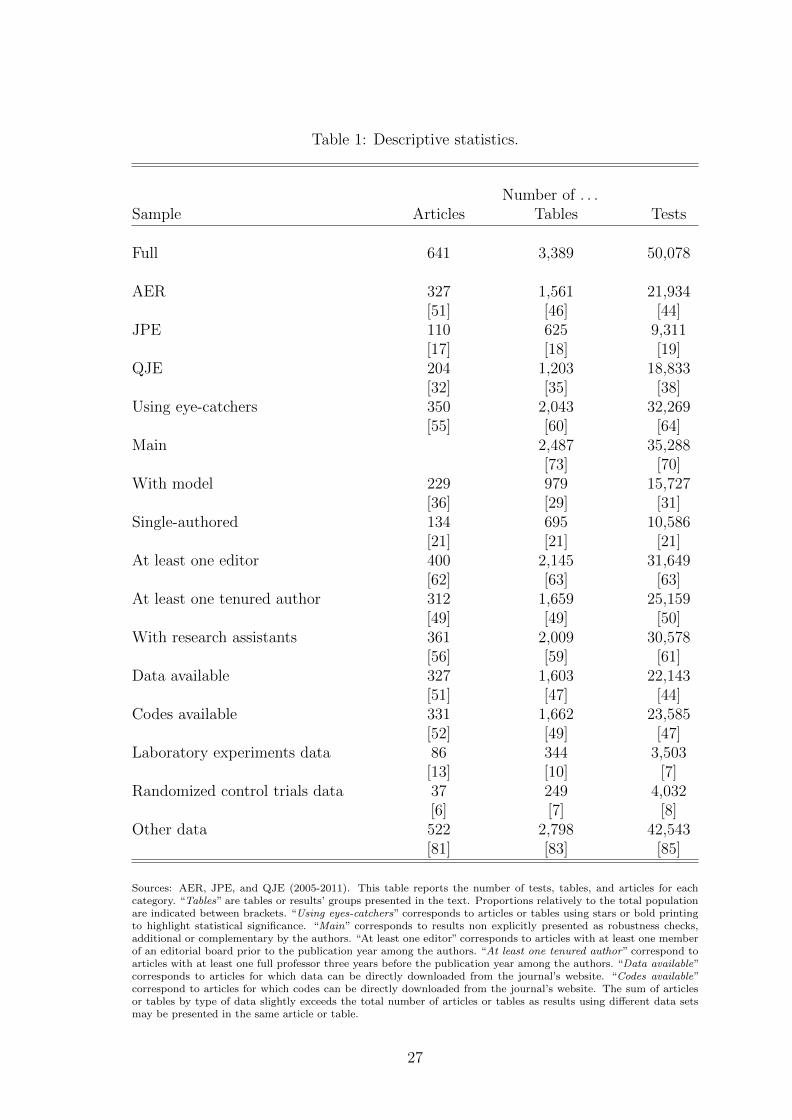
Table 1: Descriptive statistics.

Number of . . .Sample Articles Tables Tests

Full 641 3,389 50,078

AER 327 1,561 21,934[51] [46] [44]

JPE 110 625 9,311[17] [18] [19]

QJE 204 1,203 18,833[32] [35] [38]

Using eye-catchers 350 2,043 32,269[55] [60] [64]

Main 2,487 35,288[73] [70]

With model 229 979 15,727[36] [29] [31]

Single-authored 134 695 10,586[21] [21] [21]

At least one editor 400 2,145 31,649[62] [63] [63]

At least one tenured author 312 1,659 25,159[49] [49] [50]

With research assistants 361 2,009 30,578[56] [59] [61]

Data available 327 1,603 22,143[51] [47] [44]

Codes available 331 1,662 23,585[52] [49] [47]

Laboratory experiments data 86 344 3,503[13] [10] [7]

Randomized control trials data 37 249 4,032[6] [7] [8]

Other data 522 2,798 42,543[81] [83] [85]

Sources: AER, JPE, and QJE (2005-2011). This table reports the number of tests, tables, and articles for eachcategory. “Tables” are tables or results’ groups presented in the text. Proportions relatively to the total populationare indicated between brackets. “Using eyes-catchers” corresponds to articles or tables using stars or bold printingto highlight statistical significance. “Main” corresponds to results non explicitly presented as robustness checks,additional or complementary by the authors. “At least one editor” corresponds to articles with at least one memberof an editorial board prior to the publication year among the authors. “At least one tenured author” correspond toarticles with at least one full professor three years before the publication year among the authors. “Data available”corresponds to articles for which data can be directly downloaded from the journal’s website. “Codes available”correspond to articles for which codes can be directly downloaded from the journal’s website. The sum of articlesor tables by type of data slightly exceeds the total number of articles or tables as results using different data setsmay be presented in the same article or table.

27

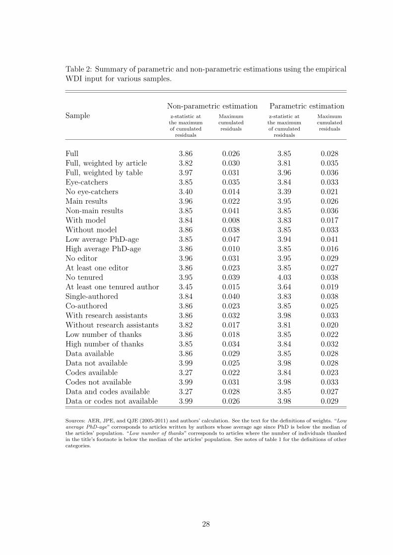
Table 2: Summary of parametric and non-parametric estimations using the empiricalWDI input for various samples.

Non-parametric estimation Parametric estimationSample z-statistic at

the maximumof cumulated

residuals

Maximumcumulatedresiduals

z-statistic atthe maximumof cumulated

residuals

Maximumcumulatedresiduals

Full 3.86 0.026 3.85 0.028Full, weighted by article 3.82 0.030 3.81 0.035Full, weighted by table 3.97 0.031 3.96 0.036Eye-catchers 3.85 0.035 3.84 0.033No eye-catchers 3.40 0.014 3.39 0.021Main results 3.96 0.022 3.95 0.026Non-main results 3.85 0.041 3.85 0.036With model 3.84 0.008 3.83 0.017Without model 3.86 0.038 3.85 0.033Low average PhD-age 3.85 0.047 3.94 0.041High average PhD-age 3.86 0.010 3.85 0.016No editor 3.96 0.031 3.95 0.029At least one editor 3.86 0.023 3.85 0.027No tenured 3.95 0.039 4.03 0.038At least one tenured author 3.45 0.015 3.64 0.019Single-authored 3.84 0.040 3.83 0.038Co-authored 3.86 0.023 3.85 0.025With research assistants 3.86 0.032 3.98 0.033Without research assistants 3.82 0.017 3.81 0.020Low number of thanks 3.86 0.018 3.85 0.022High number of thanks 3.85 0.034 3.84 0.032Data available 3.86 0.029 3.85 0.028Data not available 3.99 0.025 3.98 0.028Codes available 3.27 0.022 3.84 0.023Codes not available 3.99 0.031 3.98 0.033Data and codes available 3.27 0.028 3.85 0.027Data or codes not available 3.99 0.026 3.98 0.029

Sources: AER, JPE, and QJE (2005-2011) and authors’ calculation. See the text for the definitions of weights. “Lowaverage PhD-age” corresponds to articles written by authors whose average age since PhD is below the median ofthe articles’ population. “Low number of thanks” corresponds to articles where the number of individuals thankedin the title’s footnote is below the median of the articles’ population. See notes of table 1 for the definitions of othercategories.

28

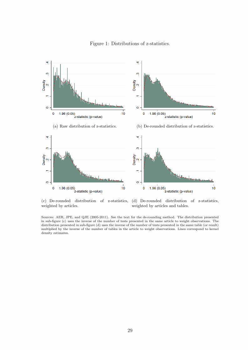
Figure 1: Distributions of z-statistics.

(a) Raw distribution of z-statistics. (b) De-rounded distribution of z-statistics.

(c) De-rounded distribution of z-statistics,weighted by articles.

(d) De-rounded distribution of z-statistics,weighted by articles and tables.

Sources: AER, JPE, and QJE (2005-2011). See the text for the de-rounding method. The distribution presentedin sub-figure (c) uses the inverse of the number of tests presented in the same article to weight observations. Thedistribution presented in sub-figure (d) uses the inverse of the number of tests presented in the same table (or result)multiplied by the inverse of the number of tables in the article to weight observations. Lines correspond to kerneldensity estimates.

29

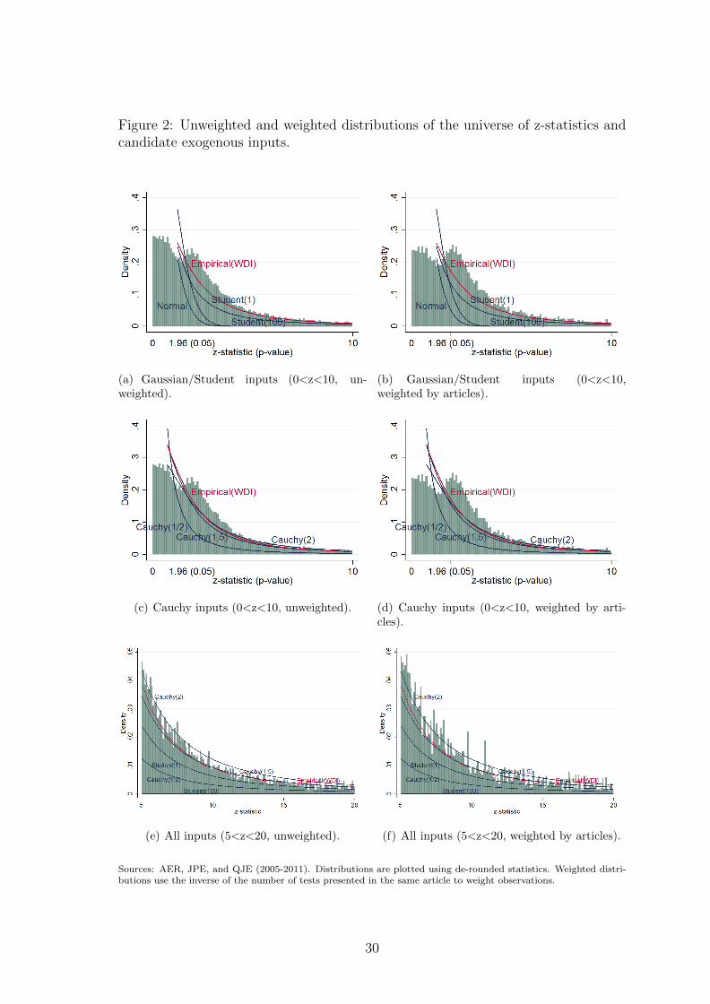
Figure 2: Unweighted and weighted distributions of the universe of z-statistics andcandidate exogenous inputs.

(a) Gaussian/Student inputs (0<z<10, un-weighted).

(b) Gaussian/Student inputs (0<z<10,weighted by articles).

(c) Cauchy inputs (0<z<10, unweighted). (d) Cauchy inputs (0<z<10, weighted by arti-cles).

(e) All inputs (5<z<20, unweighted). (f) All inputs (5<z<20, weighted by articles).

Sources: AER, JPE, and QJE (2005-2011). Distributions are plotted using de-rounded statistics. Weighted distri-butions use the inverse of the number of tests presented in the same article to weight observations.

30

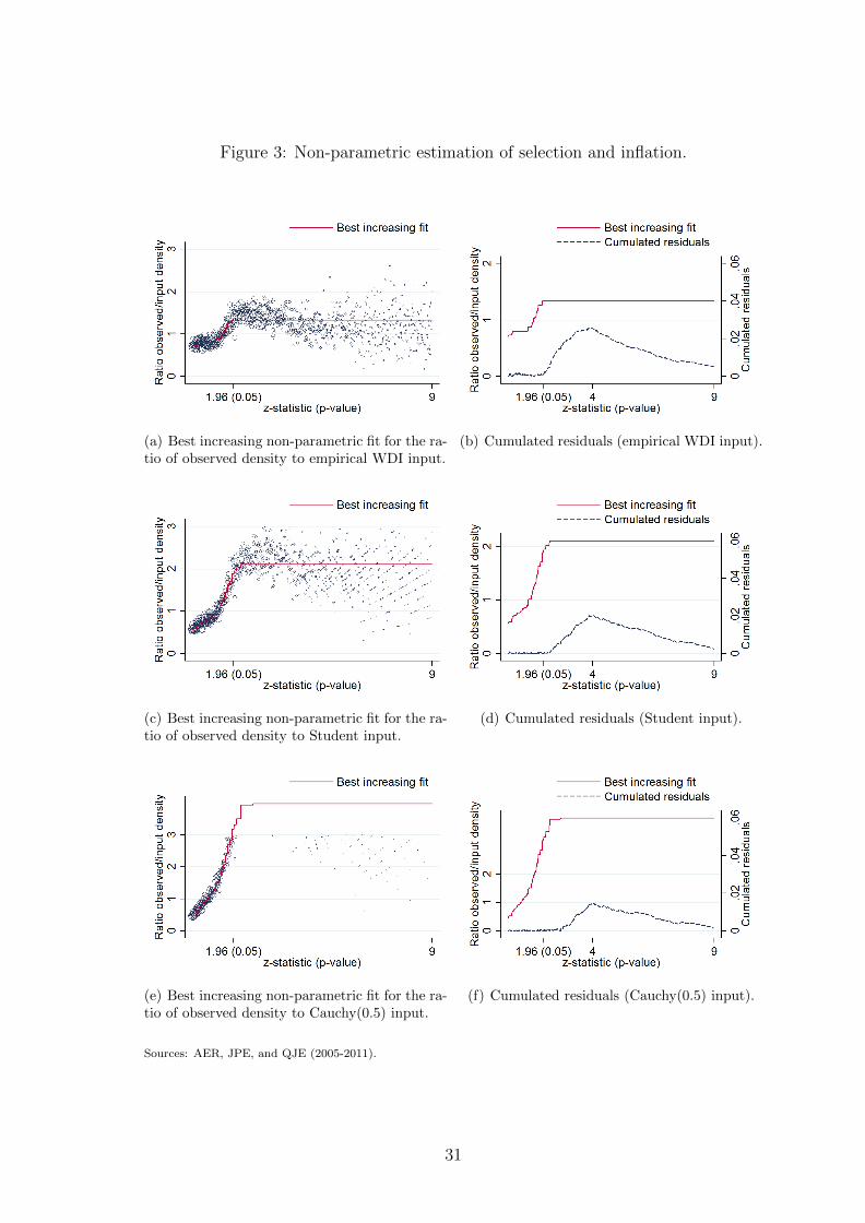
Figure 3: Non-parametric estimation of selection and inflation.

(a) Best increasing non-parametric fit for the ra-tio of observed density to empirical WDI input.

(b) Cumulated residuals (empirical WDI input).

(c) Best increasing non-parametric fit for the ra-tio of observed density to Student input.

(d) Cumulated residuals (Student input).

(e) Best increasing non-parametric fit for the ra-tio of observed density to Cauchy(0.5) input.

(f) Cumulated residuals (Cauchy(0.5) input).

Sources: AER, JPE, and QJE (2005-2011).

31

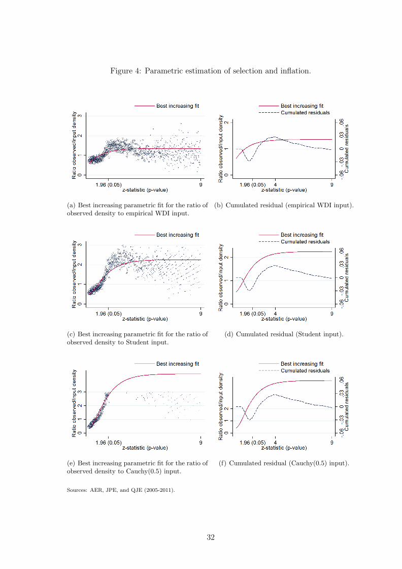
Figure 4: Parametric estimation of selection and inflation.

(a) Best increasing parametric fit for the ratio ofobserved density to empirical WDI input.

(b) Cumulated residual (empirical WDI input).

(c) Best increasing parametric fit for the ratio ofobserved density to Student input.

(d) Cumulated residual (Student input).

(e) Best increasing parametric fit for the ratio ofobserved density to Cauchy(0.5) input.

(f) Cumulated residual (Cauchy(0.5) input).

Sources: AER, JPE, and QJE (2005-2011).

32

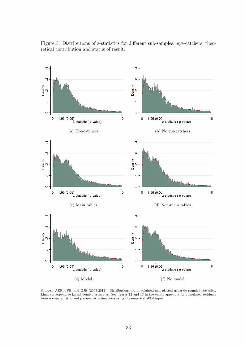
Figure 5: Distributions of z-statistics for different sub-samples: eye-catchers, theo-retical contribution and status of result.

(a) Eye-catchers. (b) No eye-catchers.

(c) Main tables. (d) Non-main tables.

(e) Model. (f) No model.

Sources: AER, JPE, and QJE (2005-2011). Distributions are unweighted and plotted using de-rounded statistics.Lines correspond to kernel density estimates. See figures 12 and 13 in the online appendix for cumulated residualsfrom non-parametric and parametric estimations using the empirical WDI input.

33

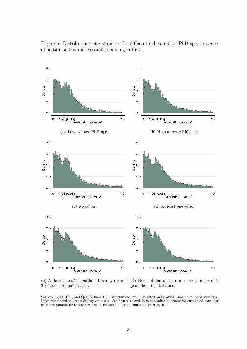
Figure 6: Distributions of z-statistics for different sub-samples: PhD-age, presenceof editors or tenured researchers among authors.

(a) Low average PhD-age. (b) High average PhD-age.

(c) No editor. (d) At least one editor

(e) At least one of the authors is surely tenured3 years before publication.

(f) None of the authors are surely tenured 3years before publication.

Sources: AER, JPE, and QJE (2005-2011). Distributions are unweighted and plotted using de-rounded statistics.Lines correspond to kernel density estimates. See figures 14 and 15 in the online appendix for cumulated residualsfrom non-parametric and parametric estimations using the empirical WDI input.

34

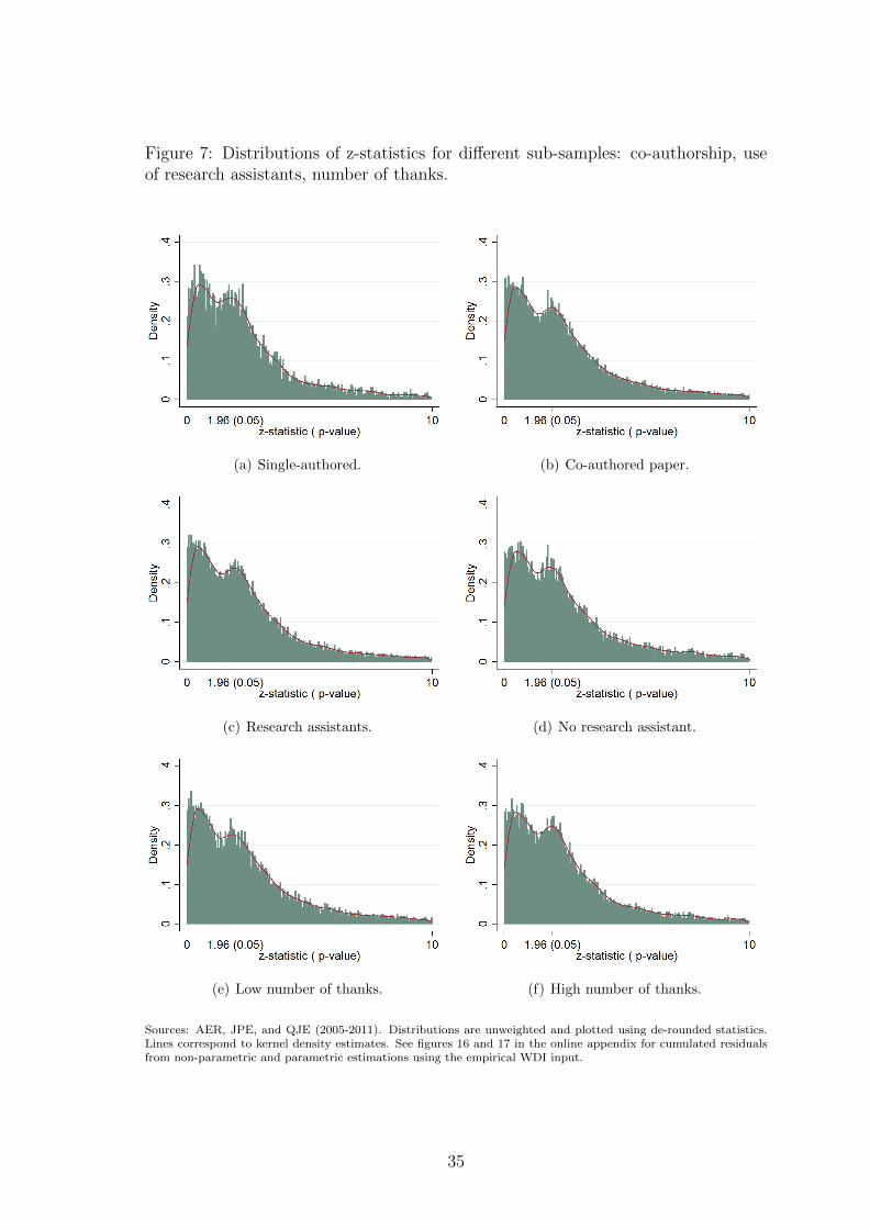
Figure 7: Distributions of z-statistics for different sub-samples: co-authorship, useof research assistants, number of thanks.

(a) Single-authored. (b) Co-authored paper.

(c) Research assistants. (d) No research assistant.

(e) Low number of thanks. (f) High number of thanks.

Sources: AER, JPE, and QJE (2005-2011). Distributions are unweighted and plotted using de-rounded statistics.Lines correspond to kernel density estimates. See figures 16 and 17 in the online appendix for cumulated residualsfrom non-parametric and parametric estimations using the empirical WDI input.

35

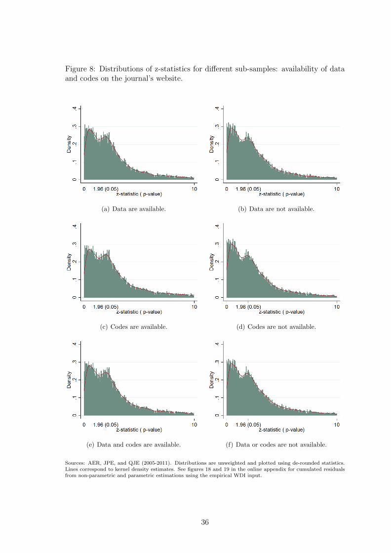
Figure 8: Distributions of z-statistics for different sub-samples: availability of dataand codes on the journal’s website.

(a) Data are available. (b) Data are not available.

(c) Codes are available. (d) Codes are not available.

(e) Data and codes are available. (f) Data or codes are not available.

Sources: AER, JPE, and QJE (2005-2011). Distributions are unweighted and plotted using de-rounded statistics.Lines correspond to kernel density estimates. See figures 18 and 19 in the online appendix for cumulated residualsfrom non-parametric and parametric estimations using the empirical WDI input.

36

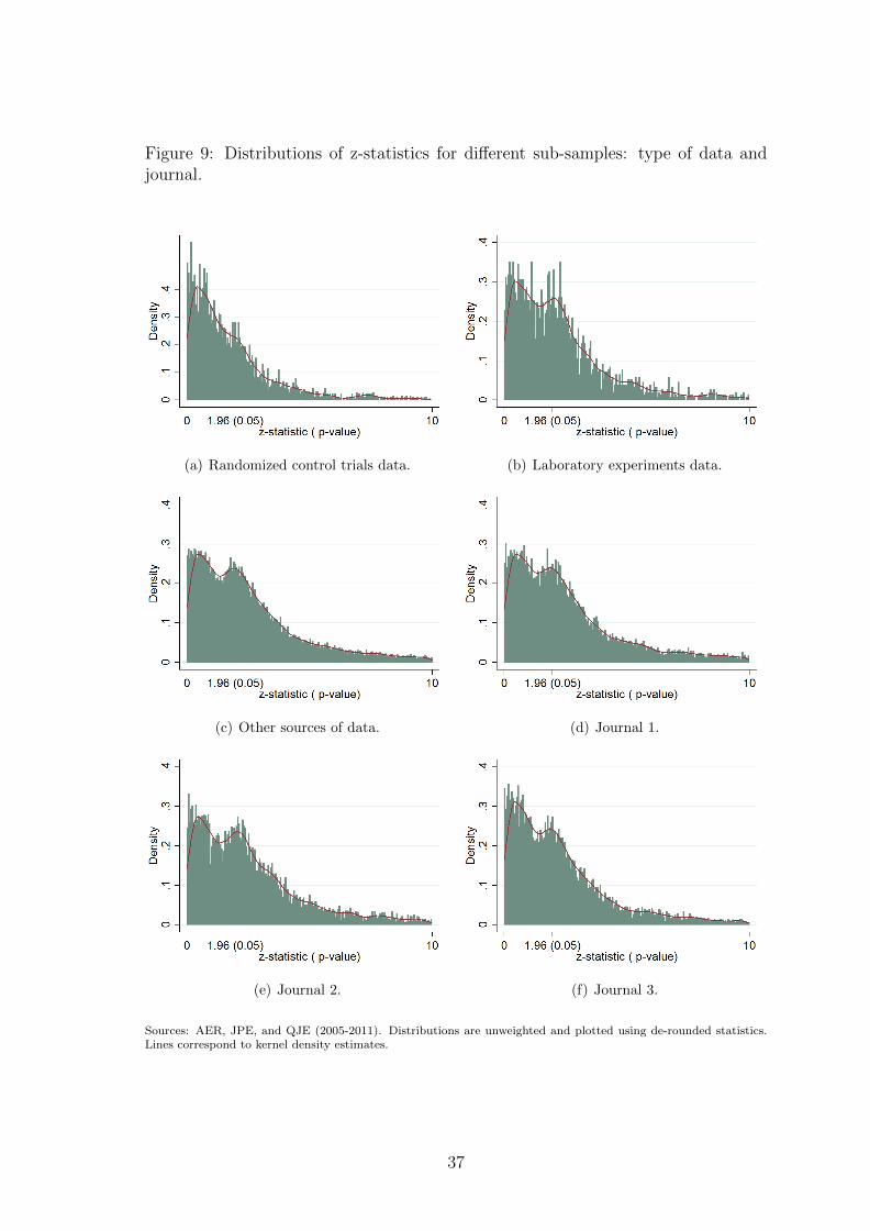
Figure 9: Distributions of z-statistics for different sub-samples: type of data andjournal.

(a) Randomized control trials data. (b) Laboratory experiments data.

(c) Other sources of data. (d) Journal 1.

(e) Journal 2. (f) Journal 3.

Sources: AER, JPE, and QJE (2005-2011). Distributions are unweighted and plotted using de-rounded statistics.Lines correspond to kernel density estimates.

37

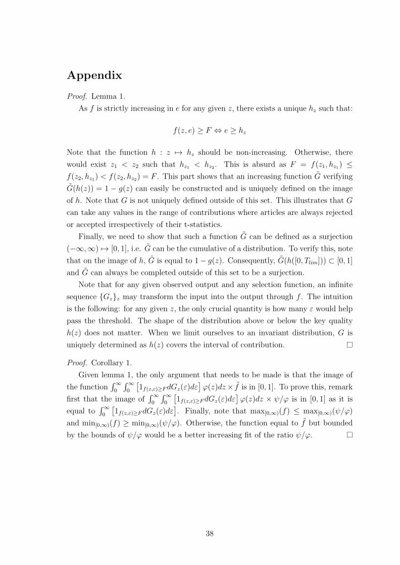
Appendix

Proof. Lemma 1.

As f is strictly increasing in e for any given z, there exists a unique hz such that:

f(z, e) ≥ F ⇔ e ≥ hz

Note that the function h : z 7→ hz should be non-increasing. Otherwise, there

would exist z1 < z2 such that hz1 < hz2 . This is absurd as F = f(z1, hz1) ≤f(z2, hz1) < f(z2, hz2) = F . This part shows that an increasing function G̃ verifying

G̃(h(z)) = 1 − g(z) can easily be constructed and is uniquely defined on the image

of h. Note that G is not uniquely defined outside of this set. This illustrates that G

can take any values in the range of contributions where articles are always rejected

or accepted irrespectively of their t-statistics.

Finally, we need to show that such a function G̃ can be defined as a surjection

(−∞,∞) 7→ [0, 1], i.e. G̃ can be the cumulative of a distribution. To verify this, note

that on the image of h, G̃ is equal to 1− g(z). Consequently, G̃(h([0, Tlim])) ⊂ [0, 1]

and G̃ can always be completed outside of this set to be a surjection.

Note that for any given observed output and any selection function, an infinite

sequence {Gz}z may transform the input into the output through f . The intuition

is the following: for any given z, the only crucial quantity is how many ε would help

pass the threshold. The shape of the distribution above or below the key quality

h(z) does not matter. When we limit ourselves to an invariant distribution, G is

uniquely determined as h(z) covers the interval of contribution.

Proof. Corollary 1.

Given lemma 1, the only argument that needs to be made is that the image of

the function∫∞

0

∫∞0

[1f(z,ε)≥FdGz(ε)dε

]ϕ(z)dz× f̃ is in [0, 1]. To prove this, remark

first that the image of∫∞

0

∫∞0

[1f(z,ε)≥FdGz(ε)dε

]ϕ(z)dz × ψ/ϕ is in [0, 1] as it is

equal to∫∞

0

[1f(z,ε)≥FdGz(ε)dε

]. Finally, note that max[0,∞)(f) ≤ max[0,∞)(ψ/ϕ)

and min[0,∞)(f) ≥ min[0,∞)(ψ/ϕ). Otherwise, the function equal to f̃ but bounded

by the bounds of ψ/ϕ would be a better increasing fit of the ratio ψ/ϕ.

38

Online appendix [For online publication]

Reporting guidelines and rules

Rules we used during the data collecting process are described below.24 The report-

ing guidelines for each information are presented in table 3.

The main idea here is to keep things very simple and transparent even if it

implies measurement errors.

• Reporting concerns articles published in the American Economic Review, the

Journal of Political Economy, and the Quarterly Journal of Economics between

2005 and 2011, except the AER Papers and Proceedings. All articles that

include at least one empirical tests should be included in the sample.

• Reporting should be done from the published version of papers.

• Report exactly what is printed in the paper. Do not allow the spreadsheet to

round anything up (this may be done by setting the data format to text before

entering data).

• Take all the variables of interest, even if authors state in the comments that

it is a good thing that a variable is not significant (an interaction term for

example). Define variables of interest by looking at the purpose of each table

and at comments of the table in the text. A rule of thumb may be that a vari-

able of interest is commented in the text alongside the paper. Explicit control

variables are not variables of interest. However, variables use to investigate

“the determinants of” something are variables of interest. When the status of

a variable of a test is unclear, be conservative and report it.

• Only report the main tables of the paper. That is, report results, but do not re-

port descriptive statistics, group comparisons, and explicit placebo tests. Only

report the tables that are commented under the headings “main results”, “ex-

tensions”, or “robustness check”. Let us impose that robustness checks and

24As highlighted in the introduction, the census of tests necessitates a good understanding ofthe argument developed in an article and a strict process avoiding any subjective selection of tests.The first observation restricts the set of potential research assistants to economists and the onlyeconomists with a sufficiently low opportunity cost were ourselves. We tackle the second issue bybeing as conservative as possible, and by avoiding interpretations of the intentions of authors.

39

extensions should be entitled as such by the authors to be considered as non-

main results. Regarding first-stages in a two-stage regression, keep only the

second-stage except if the first-stage is presented as a contribution of the paper

by itself.

• See the input mask for the reporting rules.

• For tests, fill up one spreadsheet per issue. For authors’ data, look for their

curriculum vitae using a search engine and fill up information by taking care

that some are author-invariant (such as the PhD date), but other vary with

published articles (such as status).

Example of the reporting process

Below an excerpt of an imaginary example. We only report coefficients and standard

deviations for the first variable. First-stage is not presented as a major finding by

the imaginary researchers and other variables are explicitly presented as control

variables. If the authors of this fictive table had put the last three columns in a

separate table under the heading “robustness check”, we would have considered this

new table as a “non-main” table. The table 4 presents the displayed results of this

imaginary example.

Some of the 1024 economists of our dataset engage in some project that

requires heavy data capture. It would be optimal that only individuals with

a low opportunity cost engage in such an activity. We want to investigate

the relationship between the choice of this time-consuming activity and

the intrinsic productivity of these agents in their main job. We first

estimate the relationship between data capture activity and the number

of research papers released by each economist (the number of papers is

a proxy for productivity). As shown by column 1 in table 4, there is

a significant and negative correlation between the probability to engage

in data capture and the number of written papers. However, since data

capture is a time-consuming activity, we suspect that it may also influence

the number of papers written. Thus, the average number of sunny days

per year at each department is used as an instrument for productivity.

The first-stage regression is reported in column 2 and the second stage in

column 3. The last columns reproduce the same exercise using additional

co-variates. We conclude that the decision to engage in data capture is

40

definitely negatively related to productivity. Note that controls have the

expected sign, in particular the number of co-authors.

Discontinuities

In order to test if there are any discontinuities around the thresholds of significance,

we create bins of width 0.00125 and count the number nz of z-statistics ending up in

each bin. This partition produces 1, 600 bins for approximately 20, 000 z-statistics

between 0 and 2 in the full sample.

Before turning to the results, let us detail two concerns about our capacity to

detect discontinuities. First, formal tests in an article are presented as a set of

arguments which smooth the potential discrepancy around the threshold. Second,

numbers are often roughly rounded in articles such that it is difficult to know whether

a statistic is slightly above or below a certain threshold.

Figure 20 plots nz for the full sample around 1.65 (10%) and 1.96 (5%). There

does not seem to be strong discontinuities around the thresholds. The use of a

regression around the thresholds with a trend and a quadratic term P2(z) confirms

the visual impressions. To achieve this, we estimate the following expression:

nz = γ1z>z̃ + P2(z) + εz, z ∈ [z̃ − ν, z̃ + ν].

Table 5 details the different values taken by γ along the different thresholds

z̃ ∈ {1.65, 1.96, 2.57} and the different windows ν ∈ {0.05, 0.10, 0.20, 0.30} around

the significance thresholds. The four panels of this table document the estimated dis-

continuities for the full sample, the eye-catcher sample, the no eye-catchers sample

and the eye-catcher without theoretical contribution sample.

The small number of observations in windows of width 0.10 and 0.05 does not

allow us to seize any effect in these specifications, with very high standard errors.

Nonetheless, even focusing on wider windows, the only sizable effect is at the 10%

significance threshold: γ is around .02 for samples of tests reported with eye-catchers.

Whichever the sample, the other discontinuities are never statistically different from

0. For articles using eye-catchers, the 10%-discontinuity is around 0.02. This implies

a jump of density of 0.020.24≈ 8% at the threshold.

Overall, the discontinuities are small and concentrated on articles reporting stars

and around the 10% threshold. It is to be noted that, if the experimental literature

tends to favor 1% or 5% as thresholds for rejecting the null, the vast majority of

empirical papers now considers the 10% threshold as the first level for significance.

Our results tend to illustrate the adoption of 10% as a norm.

41

These findings are of small amplitude, maybe because of the smoothing or be-

cause there are multiple tests in a same article. More importantly, even the 10%

discontinuity is hard to interpret. Authors might select tests who pass the signifi-

cance thresholds among the set of acceptable specifications and only show part of

the whole range of inferences. But it might also be that journals prefer significant

results or authors censor themselves, expecting journals to be harsher with unsignif-

icant results.

An extension to the Benford’s law

Following the seminal paper of Benford (1938) and its extension by Hill (1995, 1998),

the leading digit of numbers taken from scale-invariant data or selected from a lot

of different sources should follow a logarithmic distribution. Tests of this law are

applied to situations such as tax monitoring in order to see whether reported figures

are manipulated or not.

The intuition is that we are in the precise situation in which the Benford’s law

should hold: we group coefficients from different sources, with different units and

thus different scales. According to Hill (1995, 1998), the probability for one of our

collected coefficients to have a leading digit equal to d ∈ {0, . . . , 9} is log10(1 + 1/d).

We group coefficients and standard deviations taken from our different articles

(with different units). z-statistics are not used in this analysis as it is not scale-

invariant and normalized across the different articles. For both coefficients and

standard errors, we compute the empirical probability rd to have a leading digit

equal to d ∈ {0, . . . , 9}.The first columns of table 6 (panel A for the coefficients, panel B for the standard

errors) display the theoretical probabilities and the empirical counterparts for three

samples: the full sample, the sample of coefficients and standard errors for which

the associated z-statistic was in the [1.65, 6] interval, and the others. All samples

seem incredibly close to the theoretical predictions. The distance to the theoretical

prediction can be summarized by the statistic U =√∑∞

d=1(rd − log10(1 + 1/d))2.

A concern is that we have no benchmark upon which we can rely: the distance

to the theoretical prediction seems small but it may be because of the very large

number of observations. We re-use our random regressions on WDI, and randomly

extract approximately as many coefficients and standard deviations as in the real

sample. We already know that the distribution of z-statistics are quite close; the

decomposition of coefficients and standard errors with z-statistics between 1.65 and

6 should partition the placebo sample in similar proportions as the real sample. The

three last columns of panels A and B present the results on this placebo sample.

42

The comparison of the two sets of results indicates that the distance of the

full sample to the theoretical predictions is higher than with the placebo both for

coefficients (Us = 0.0089 against Up = 0.0058) and for standard errors (Us = 0.0117

against Up = 0.0046). The analysis across subsample is less straightforward. As

regards the coefficients, the relative distance compared to the placebo is particularly

large between 1.65 and 6 (Us = 0.0161 against Up = 0.0036 for the [1.65, 6] sample,

and Us = 0.0081 against Up = 0.0093 for the rest). It seems however that this

observation does not hold for standard errors. Naturally, part of this discrepancy

can be explained by the differences in the number of observations: there are less

numbers reported between 1.65 and 6 in the placebo test. To conclude, this Benford

analysis provides some evidence indicating non-randomness in our universe of tests.

43

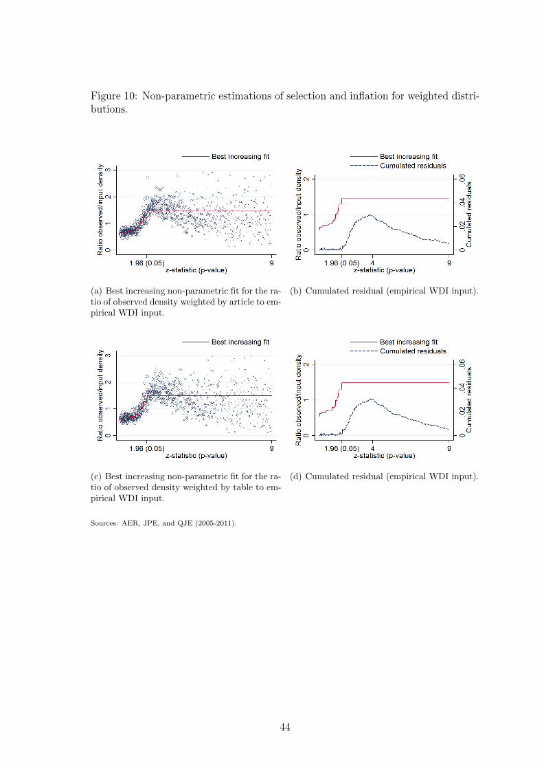
Figure 10: Non-parametric estimations of selection and inflation for weighted distri-butions.

(a) Best increasing non-parametric fit for the ra-tio of observed density weighted by article to em-pirical WDI input.

(b) Cumulated residual (empirical WDI input).

(c) Best increasing non-parametric fit for the ra-tio of observed density weighted by table to em-pirical WDI input.

(d) Cumulated residual (empirical WDI input).

Sources: AER, JPE, and QJE (2005-2011).

44

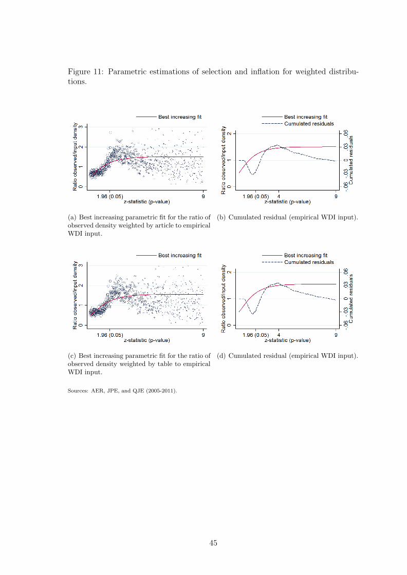
Figure 11: Parametric estimations of selection and inflation for weighted distribu-tions.

(a) Best increasing parametric fit for the ratio ofobserved density weighted by article to empiricalWDI input.

(b) Cumulated residual (empirical WDI input).

(c) Best increasing parametric fit for the ratio ofobserved density weighted by table to empiricalWDI input.

(d) Cumulated residual (empirical WDI input).

Sources: AER, JPE, and QJE (2005-2011).

45

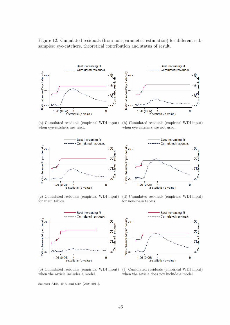
Figure 12: Cumulated residuals (from non-parametric estimation) for different sub-samples: eye-catchers, theoretical contribution and status of result.

(a) Cumulated residuals (empirical WDI input)when eye-catchers are used.

(b) Cumulated residuals (empirical WDI input)when eye-catchers are not used.

(c) Cumulated residuals (empirical WDI input)for main tables.

(d) Cumulated residuals (empirical WDI input)for non-main tables.

(e) Cumulated residuals (empirical WDI input)when the article includes a model.

(f) Cumulated residuals (empirical WDI input)when the article does not include a model.

Sources: AER, JPE, and QJE (2005-2011).

46

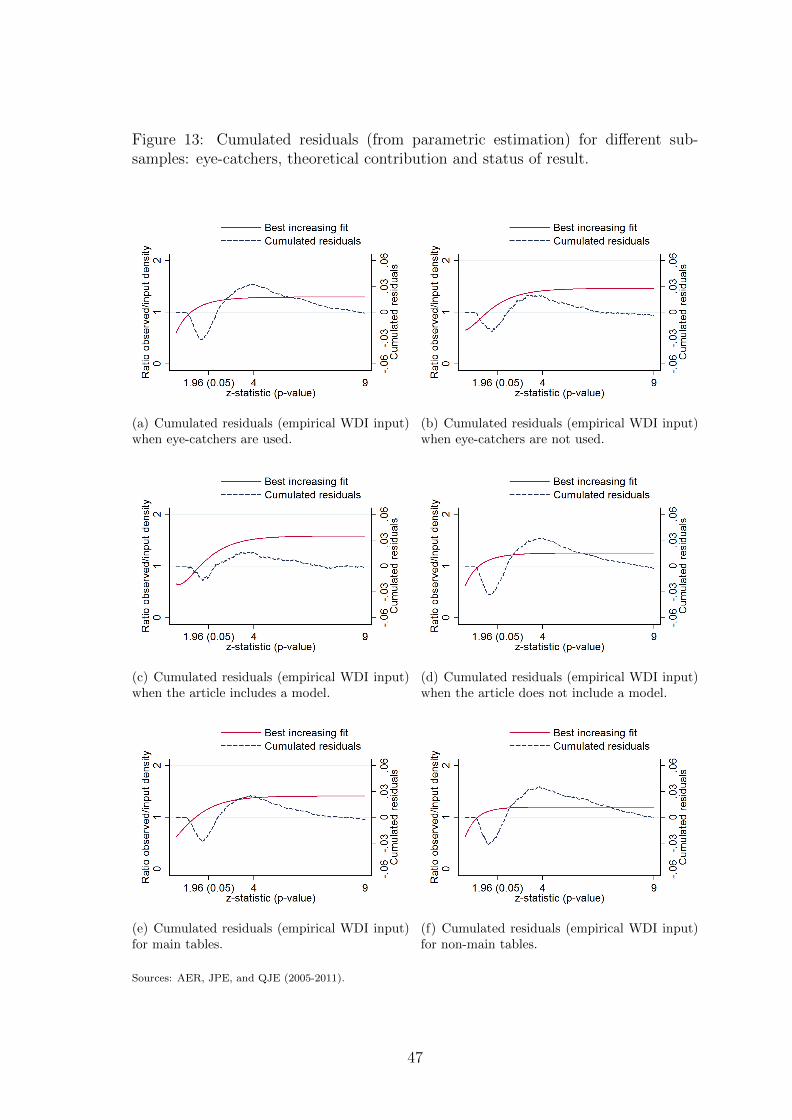
Figure 13: Cumulated residuals (from parametric estimation) for different sub-samples: eye-catchers, theoretical contribution and status of result.

(a) Cumulated residuals (empirical WDI input)when eye-catchers are used.

(b) Cumulated residuals (empirical WDI input)when eye-catchers are not used.

(c) Cumulated residuals (empirical WDI input)when the article includes a model.

(d) Cumulated residuals (empirical WDI input)when the article does not include a model.

(e) Cumulated residuals (empirical WDI input)for main tables.

(f) Cumulated residuals (empirical WDI input)for non-main tables.

Sources: AER, JPE, and QJE (2005-2011).

47

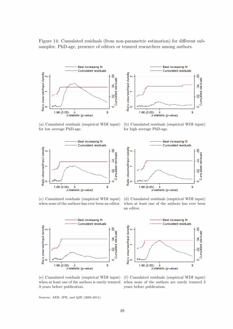
Figure 14: Cumulated residuals (from non-parametric estimation) for different sub-samples: PhD-age, presence of editors or tenured researchers among authors.

(a) Cumulated residuals (empirical WDI input)for low average PhD-age.

(b) Cumulated residuals (empirical WDI input)for high average PhD-age.

(c) Cumulated residuals (empirical WDI input)when none of the authors has ever been an editor.

(d) Cumulated residuals (empirical WDI input)when at least one of the authors has ever beenan editor.

(e) Cumulated residuals (empirical WDI input)when at least one of the authors is surely tenured3 years before publication.

(f) Cumulated residuals (empirical WDI input)when none of the authors are surely tenured 3years before publication.

Sources: AER, JPE, and QJE (2005-2011).

48

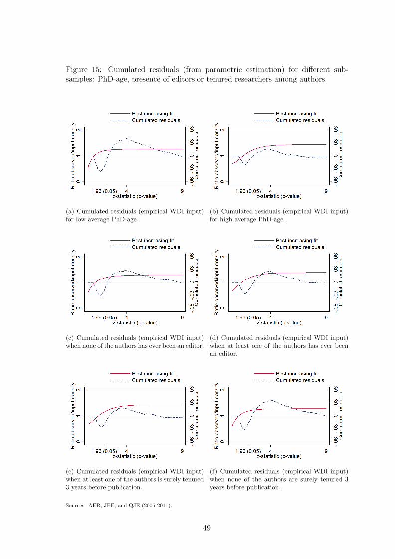
Figure 15: Cumulated residuals (from parametric estimation) for different sub-samples: PhD-age, presence of editors or tenured researchers among authors.

(a) Cumulated residuals (empirical WDI input)for low average PhD-age.

(b) Cumulated residuals (empirical WDI input)for high average PhD-age.

(c) Cumulated residuals (empirical WDI input)when none of the authors has ever been an editor.

(d) Cumulated residuals (empirical WDI input)when at least one of the authors has ever beenan editor.

(e) Cumulated residuals (empirical WDI input)when at least one of the authors is surely tenured3 years before publication.

(f) Cumulated residuals (empirical WDI input)when none of the authors are surely tenured 3years before publication.

Sources: AER, JPE, and QJE (2005-2011).

49

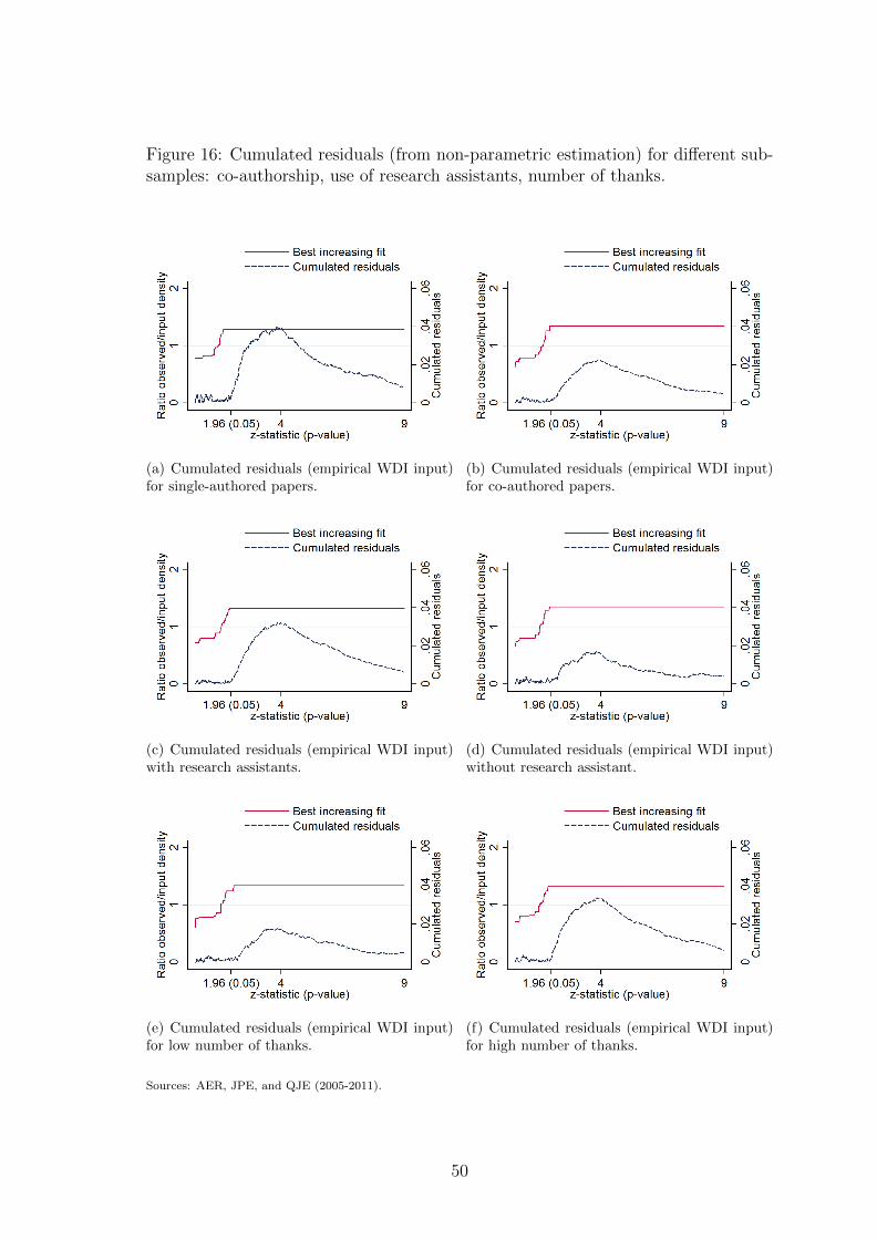
Figure 16: Cumulated residuals (from non-parametric estimation) for different sub-samples: co-authorship, use of research assistants, number of thanks.

(a) Cumulated residuals (empirical WDI input)for single-authored papers.

(b) Cumulated residuals (empirical WDI input)for co-authored papers.

(c) Cumulated residuals (empirical WDI input)with research assistants.

(d) Cumulated residuals (empirical WDI input)without research assistant.

(e) Cumulated residuals (empirical WDI input)for low number of thanks.

(f) Cumulated residuals (empirical WDI input)for high number of thanks.

Sources: AER, JPE, and QJE (2005-2011).

50

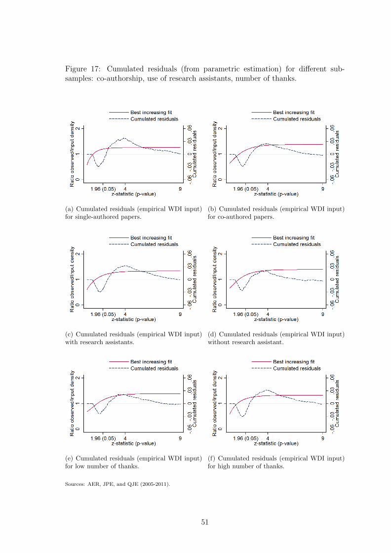
Figure 17: Cumulated residuals (from parametric estimation) for different sub-samples: co-authorship, use of research assistants, number of thanks.

(a) Cumulated residuals (empirical WDI input)for single-authored papers.

(b) Cumulated residuals (empirical WDI input)for co-authored papers.

(c) Cumulated residuals (empirical WDI input)with research assistants.

(d) Cumulated residuals (empirical WDI input)without research assistant.

(e) Cumulated residuals (empirical WDI input)for low number of thanks.

(f) Cumulated residuals (empirical WDI input)for high number of thanks.

Sources: AER, JPE, and QJE (2005-2011).

51

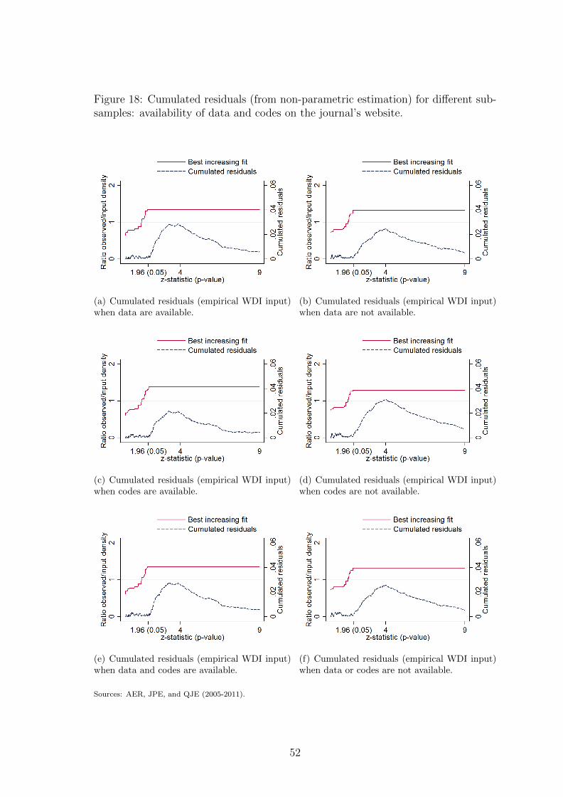
Figure 18: Cumulated residuals (from non-parametric estimation) for different sub-samples: availability of data and codes on the journal’s website.

(a) Cumulated residuals (empirical WDI input)when data are available.

(b) Cumulated residuals (empirical WDI input)when data are not available.

(c) Cumulated residuals (empirical WDI input)when codes are available.

(d) Cumulated residuals (empirical WDI input)when codes are not available.

(e) Cumulated residuals (empirical WDI input)when data and codes are available.

(f) Cumulated residuals (empirical WDI input)when data or codes are not available.

Sources: AER, JPE, and QJE (2005-2011).

52

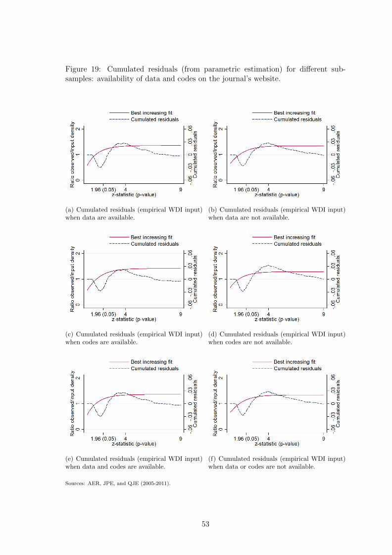
Figure 19: Cumulated residuals (from parametric estimation) for different sub-samples: availability of data and codes on the journal’s website.

(a) Cumulated residuals (empirical WDI input)when data are available.

(b) Cumulated residuals (empirical WDI input)when data are not available.

(c) Cumulated residuals (empirical WDI input)when codes are available.

(d) Cumulated residuals (empirical WDI input)when codes are not available.

(e) Cumulated residuals (empirical WDI input)when data and codes are available.

(f) Cumulated residuals (empirical WDI input)when data or codes are not available.

Sources: AER, JPE, and QJE (2005-2011).

53

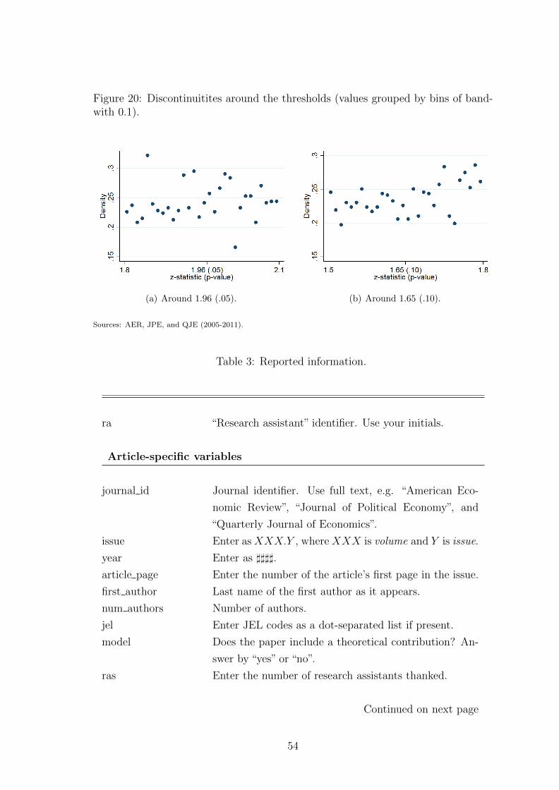
Figure 20: Discontinuitites around the thresholds (values grouped by bins of band-with 0.1).

(a) Around 1.96 (.05). (b) Around 1.65 (.10).

Sources: AER, JPE, and QJE (2005-2011).

Table 3: Reported information.

ra “Research assistant” identifier. Use your initials.

Article-specific variables

journal id Journal identifier. Use full text, e.g. “American Eco-

nomic Review”, “Journal of Political Economy”, and

“Quarterly Journal of Economics”.

issue Enter asXXX.Y , whereXXX is volume and Y is issue.

year Enter as ]]]].

article page Enter the number of the article’s first page in the issue.

first author Last name of the first author as it appears.

num authors Number of authors.

jel Enter JEL codes as a dot-separated list if present.

model Does the paper include a theoretical contribution? An-

swer by “yes” or “no”.

ras Enter the number of research assistants thanked.

Continued on next page

54

Table 3: Reported information (continued).

thanks Enter the number of individuals thanked (excluding re-

search assistant and referees).

Test-specific variables

type Type of data used. Three choices: “expe” for experi-

mental data, “rct” for data obtained from randomized

control trials, and “other” for any other type of data.

table panel Enter the table identifier. If a table includes several

parts (e.g. panels), also enter the panel identifier. In

case where results are presented only in the text, create

a separate identifier for each “group” of results in the

paper.

type emp Statistical method or type of test used.

row Row identifier when referring to a table. Enter the page

number when referring to results presented in the text.

column Column identifier when referring to a table. Enter the

order of appearance when referring to results presented

in the text.

stars Does the paper use eye-catchers (e.g. stars or bold print-

ing) to highlight statistical significance? Answer by“yes”

or “no”.

main Enter “yes” or “no”. For simplicity, assign the same

status to all tests presented in the same table or re-

sults’group.

coefficient Enter the coefficient.

standard deviation Enter the standard deviation. Create a variable

called “standard deviation 2” if authors reported mul-

tiple standard deviations (e.g. first is clustered, the sec-

ond is not).

t stat Enter the test statistic. Create a variable called

“t stat 2” if authors reported multiple statistics.

p value Enter the p-value. Create a variable called “p value 2”

if authors reported multiple p-values.

Continued on next page

55

Table 3: Reported information (continued).

Author-specific variables

phd PhD institution. Enter “Unknown” if you cannot find

the information.

phd date Enter as ]]]] the year at which the PhD was awarded.

Enter the expected date if necessary. Enter “Unknown”

if you cannot find the information.

Author×article-specific variables

author Author’s name

status Enter the status of the author at time of publication.

Enter “Unknown” if you cannot find the information.

status 1y Enter the status of the author one year before publica-

tion.

status 2y Enter the status of the author two years before publica-

tion.

status 3y Enter the status of the author three years before publi-

cation.

editor Is the author an editor or a member of an editorial board

at time of publication? Answer by “yes” or “no”. Enter

“Unknown” if you cannot find the information.

editor before Was the author an editor or a member of an editorial

board before publication? Answer by “yes” or “no”.

affiliation 1 Enter the author’s first affiliation as it appears on the

published version of the article.

affiliation 2 Enter the author’s other affiliations as they appear on

the published version of the article.

56

Table 4: Imaginary example: Activity choice and productivity among economists.

(1) (2) (3) (4) (5) (6)OLS First stage IV OLS First stage IV

Dependent variable: Data capture Papers Data capture Data capture Papers Data capture

Papers -0.183*** -0.190 -0.189*** -0.243*(0.024) (0.162) (0.018) (0.134)

Sunny days -0.360*** -0.372***(0.068) (0.068)

Gender -0.028 0.090** -0.067**(0.023) (0.039) (0.031)

Size of department -0.000 0.001 -0.000(0.001) (0.002) (0.002)

Number of co-authors 0.223*** 0.004 0.222***(0.008) (0.014) (0.010)

Country fixed effects Yes Yes Yes

Observations 1,024 1,024 1,024 1,024 1,024 1,024R-squared 0.054 0.027 0.475 0.042

*** p<0.01, ** p<0.05, * p<0.1. Standard errors in parentheses. Data are imaginary. The model is a linearprobability model estimated with ordinary least squares. Data capture is a dummy equal to 1 if the economistcaptures data. Papers is the number of papers (including working papers). Sunny days is the number of sunny daysper year at each department. Size of the department is the size of the department. Number of co-authors is thenumber of co-authors. In columns 3 and 6, papers is instrumented by sunny days. All regressions include a constantterm.

57

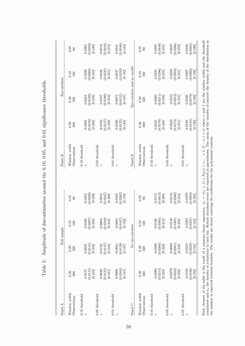
Tab

le5:

Am

plitu

de

ofdis

conti

nuit

ies

arou

nd

the

0.10

,0.

05,

and

0.01

sign

ifica

nce

thre

shol

ds.

Pan

elA

Fu

llsa

mp

leP

an

elB

Eye-

catc

her

s

Win

dow

wid

th0.3

00.2

00.1

00.0

5W

indow

wid

th0.3

00.2

00.1

00.0

5O

bse

rvati

on

s480

320

160

80

Obse

rvati

on

s480

320

160

80

0.1

0th

resh

old

0.1

0th

resh

old

γ0.0

157

0.0

033

0.0

168

0.0

262

γ0.0

268

0.0

204

0.0

206

0.0

365

(0.0

115)

(0.0

144)

(0.0

207)

(0.0

330)

(0.0

150)

(0.0

186)

(0.0

266)

(0.0

393)

[0.2

32]

[0.2

32]

[0.2

32]

[0.2

28]

[0.2

38]

[0.2

38]

[0.2

42]

[0.2

40]

0.0

5th

resh

old

0.0

5th

resh

old

γ0.0

049

0.0

152

0.0

064

0.0

015

γ0.0

160

0.0

187

0.0

106

0.0

018

(0.0

121)

(0.0

147)

(0.0

189)

(0.0

247)

(0.0

147)

(0.0

180)

(0.0

235)

(0.0

310)

[0.2

41]

[0.2

44]

[0.2

42]

[0.2

60]

[0.2

48]

[0.2

53]

[0.2

51]

[0.2

73]

0.0

1th

resh

old

0.0

1th

resh

old

γ0.0

009

-0.0

051

-0.0

061

0.0

103

γ0.0

106

0.0

075

0.0

047

0.0

341

(0.0

104)

(0.0

129)

(0.0

187)

(0.0

263)

(0.0

125)

(0.0

155)

(0.0

232)

(0.0

348)

[0.1

87]

[0.1

87]

[0.1

82]

[0.1

76]

[0.1

88]

[0.1

87]

[0.1

82]

[0.1

84]

Pan

elC

No

eye-

catc

her

sP

anel

DE

ye-

catc

her

san

dn

om

od

el

Win

dow

wid

th0.3

00.2

00.1

00.0

5W

indow

wid

th0.3

00.2

00.1

00.0

5O

bse

rvati

on

s480

320

160

80

Obse

rvati

on

s480

320

160

80

0.1

0th

resh

old

0.1

0th

resh

old

γ-0

.0086

-0.0

306

0.0

130

0.0

113

γ0.0

225

0.0

280

0.0

295

0.0

293

(0.0

214)

(0.0

266)

(0.0

385)

(0.0

613)

(0.0

170)

(0.0

211)

(0.0

296)

(0.0

448)

[0.2

25]

[0.2

23]

[0.2

13]

[0.2

04]

[0.2

46]

[0.2

48]

[0.2

55]

[0.2

55]

0.0

5th

resh

old

0.0

5th

resh

old

γ-0

.0279

-0.0

003

-0.0

148

-0.0

116

γ-0

.0048

-0.0

152

-0.0

223

-0.0

637

(0.0

222)

(0.0

281)

(0.0

405)

(0.0

586)

(0.0

173)

(0.0

212)

(0.0

284)

(0.0

386)

[0.2

30]

[0.2

32]

[0.2

32]

[0.2

44]

[0.2

51]

[0.2

54]

[0.2

51]

[0.2

72]

0.0

1th

resh

old

0.0

1th

resh

old

γ-0

.0192

-0.0

253

-0.0

284

-0.0

379

γ0.0

160

0.0

236

0.0

287

0.0

420

(0.0

186)

(0.0

229)

(0.0

331)

(0.0

504)

(0.0

145)

(0.0

179)

(0.0

260)

(0.0

385)

[0.1

92]

[0.1

91]

[0.1

84]

[0.1

65]

[0.1

90]

[0.1

90]

[0.1

86]

[0.1

90]

Each

elem

ent

of

the

tab

leis

the

resu

ltof

ase

para

telin

ear

regre

ssio

n.nz

=γ

(z>z̃)

+P2(z

)+ε z,

z∈

[z̃−ν,z̃

+ν]

wh

ereν

andz̃

are

the

win

dow

wid

thand

the

thre

shold

con

sid

ered

an

dnz

the

den

sity

of

z-st

ati

stic

sin

each

bin

.R

ob

ust

stan

dard

erro

rsare

rep

ort

edin

pare

nth

eses

.T

he

mea

nof

the

vari

able

of

inte

rest

–th

ed

ensi

tyof

the

dis

trib

uti

on

inth

ew

ind

ow

–is

rep

ort

edb

etw

een

bra

cket

s.T

he

resu

lts

are

show

nom

itti

ng

the

coeffi

cien

tsfo

rth

ep

oly

nom

ial

contr

ols

.

58

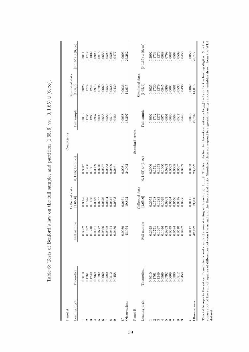
Tab

le6:

Tes

tsof

Ben

ford

’sla

won

the

full

sam

ple

,an

dpar

titi

on[1.6

5,6]

vs.

[0,1.6

5)∪

(6,∞

).

Pan

elA

Coeffi

cien

tsC

ollec

ted

data

Sim

ula

ted

data

Lea

din

gd

igit

Theo

reti

cal

Fu

llsa

mp

le[1.6

5,6

][0,1.6

5)∪

(6,∞

)F

ull

sam

ple

[1.6

5,6

][0,1.6

5)∪

(6,∞

)

10.3

010

0.3

052

0.3

095

0.3

017

0.3

016

0.3

026

0.3

011

20.1

761

0.1

692

0.1

675

0.1

706

0.1

735

0.1

774

0.1

717

30.1

249

0.1

240

0.1

166

0.1

301

0.1

283

0.1

244

0.1

302

40.0

969

0.0

981

0.0

972

0.0

989

0.0

937

0.0

973

0.0

920

50.0

792

0.0

772

0.0

767

0.0

776

0.0

809

0.0

796

0.0

816

60.0

669

0.0

666

0.0

676

0.0

657

0.0

658

0.0

669

0.0

653

70.0

580

0.0

592

0.0

604

0.0

583

0.0

586

0.0

559

0.0

599

80.0

512

0.0

524

0.0

542

0.0

509

0.0

510

0.0

520

0.0

506

90.0

458

0.0

480

0.0

503

0.0

461

0.0

464

0.0

439

0.0

477

U0.0

089

0.0

161

0.0

081

0.0

058

0.0

036

0.0

093

Obse

rvati

on

s43,9

54

19,8

92

24,0

62

43,2

97

14,0

15

29,2

82

Pan

elB

Sta

nd

ard

erro

rsC

ollec

ted

data

Sim

ula

ted

data

Lea

din

gd

igit

Theo

reti

cal

Fu

llsa

mp

le[1.6

5,6

][0,1.6

5)∪

(6,∞

)F

ull

sam

ple

[1.6

5,6

][0,1.6

5)∪

(6,∞

)

10.3

010

0.2

928

0.2

955

0.2

906

0.3

002

0.3

025

0.2

992

20.1

761

0.1

751

0.1

798

0.1

711

0.1

732

0.1

730

0.1

733

30.1

249

0.1

267

0.1

283

0.1

253

0.1

277

0.1

279

0.1

276

40.0

969

0.1

046

0.1

029

0.1

060

0.0

974

0.0

945

0.0

988

50.0

792

0.0

803

0.0

803

0.0

803

0.0

801

0.0

808

0.0

798

60.0

669

0.0

649

0.0

634

0.0

662

0.0

680

0.0

664

0.0

687

70.0

580

0.0

584

0.0

556

0.0

608

0.0

569

0.0

581

0.0

564

80.0

512

0.0

510

0.0

478

0.0

537

0.0

517

0.0

533

0.0

509

90.0

458

0.0

462

0.0

466

0.0

459

0.0

448

0.0

436

0.0

453

U0.0

117

0.0

111

0.0

153

0.0

046

0.0

062

0.0

053

Obse

rvati

on

s42,4

22

19,2

00

23,2

22

42,7

92

14,0

15

28,7

77

This

table

rep

ort

sth

era

tios

of

coeffi

cien

tsan

dst

and

ard

erro

rsst

art

ing

wit

hea

chd

igit

1,...,9

.T

he

form

ula

for

the

theo

reti

cal

rati

os

islo

g10(1

+1/d)

for

the

lead

ing

dig

itd.U

isth

esq

uare

root

of

the

sum

of

squ

are

sof

diff

eren

ces

bet

wee

nth

eact

ual

and

the

theo

reti

cal

rati

o.

Sim

ula

ted

data

corr

esp

on

dto

regre

ssio

ns

usi

ng

ran

dom

vari

able

sd

raw

nfr

om

the

WD

Id

ata

set.

59