Embed Size (px)
DESCRIPTION
Economic Growth paper
Citation preview
Growth Empirics: A Panel Data ApproachAuthor(s): Nazrul IslamSource: The Quarterly Journal of Economics, Vol. 110, No. 4 (Nov., 1995), pp. 1127-1170Published by: Oxford University PressStable URL: http://www.jstor.org/stable/2946651 .
Accessed: 25/04/2014 17:43
Your use of the JSTOR archive indicates your acceptance of the Terms & Conditions of Use, available at .http://www.jstor.org/page/info/about/policies/terms.jsp
.JSTOR is a not-for-profit service that helps scholars, researchers, and students discover, use, and build upon a wide range ofcontent in a trusted digital archive. We use information technology and tools to increase productivity and facilitate new formsof scholarship. For more information about JSTOR, please contact [email protected].
.
Oxford University Press is collaborating with JSTOR to digitize, preserve and extend access to The QuarterlyJournal of Economics.
http://www.jstor.org
This content downloaded from 143.107.92.181 on Fri, 25 Apr 2014 17:43:38 PMAll use subject to JSTOR Terms and Conditions
GROWTH EMPIRICS: A PANEL DATA APPROACH*
NAZRUL ISLAM
A panel data approach is advocated and implemented for studying growth convergence. The familiar equation for testing convergence is reformulated as a dynamic panel data model, and different panel data estimators are used to estimate it. The main usefulness of the panel approach lies in its ability to allow for differences in the aggregate production function across economies. This leads to results that are significantly different from those obtained from single cross- country regressions. In the process of identifying the individual "country effect," we can also see the point where neoclassical growth empirics meets development economics.
I. INTRODUCTION
In recent years there has been considerable empirical work on cross-country growth. A close two-way relationship has been observed between this work and the corresponding developments in the theory of growth, in particular, the emergence of new (endogenous) growth theories and the ensuing conflict between these on the one hand and the preexisting models of growth in the tradition of Solow [1956], Cass [1965], and Koopmans [1965], on the other. A central focus of this work has been the issue of convergence. While the finding of convergence has been generally thought of as evidence in support of the Solow-Cass-Koopmans model, absence of convergence has been regarded as supportive of endogenous growth theories. The controversy has given rise to the concept of "conditional convergence" meaning convergence after differences in the steady states across countries have been con- trolled for.
A common feature of existing empirical studies on this issue has been the assumption of identical aggregate production func- tions for all the countries. Although it has been correctly felt that the production function may actually differ across countries, efforts at allowing for such differences have been limited by the fact that most of these studies have been conducted in the framework of single cross-country regressions. In this framework it is econometri-
*I would like to thank Dale W. Jorgenson, Gary Chamberlain, Guido W. Imbens, Robert M. Solow, James H. Stock, Lawrence F. Katz, Olivier J. Blanchard, and an anonymous referee for their helpful suggestions. I also benefited from the comments of Xoce Garcia, Eduard Sprokholt, and participants of the Harvard Econometrics Lunch. All remaining errors are mine.
? 1995 by the President and Fellows of Harvard College and the Massachusetts Institute of Technology. The Quarterly Journal of Economics, November 1995
This content downloaded from 143.107.92.181 on Fri, 25 Apr 2014 17:43:38 PMAll use subject to JSTOR Terms and Conditions
1128 QUARTERLY JOURNAL OF ECONOMICS
cally difficult to allow for such differences in the production function as are not (easily) measurable.
The present paper advocates and implements a panel data approach to deal with this issue. The panel data framework makes it possible to allow for differences of the above-mentioned type in the form of unobservable individual "country effects." This paper takes the recent work by Mankiw, Romer, and Weil [1992] as its starting point and examines how the results change with the adoption of the panel data approach. We reformulate the regres- sion equation used in the study of convergence into a dynamic panel data model with individual (country) effects and use the panel data procedures to estimate it. This yields results that are different from the corresponding results obtained from single cross-section methodology. First, the estimated rates of conditional convergence prove to be higher. Second, the estimated values of the elasticity of output with respect to capital are found to be much lower and more in conformity with its commonly accepted empiri- cal values.
Investigation into the statistical sources of the aforemen- tioned changes in the results shows that both of them can, to a great extent, be explained in the framework of omitted variable bias. The country-specific aspect of the aggregate production function that is ignored in single cross-section regression, is correlated with the included explanatory variables, and this creates omitted variable bias. The panel data framework makes it possible to correct this bias. From growth theory's point of view, the panel approach allows us to isolate the effect of "capital deepening" on the one hand and technological and institutional differences on the other, in the process of convergence. The results indicate that persistent differences in technology level and institutions are a significant factor in understanding cross-country economic growth. It becomes clear that if there had been no such differences, and countries differed only in terms of capital per capita, convergence would have proceeded at a faster rate.
Contrary to what may appear at first sight, the finding of a higher rate of conditional convergence actually calls for more policy activism. In the setup of identical production functions, in order to increase the steady state level of per capita income, countries were to focus only on the rates of saving and labor force growth. But when differences in the aggregate production function are allowed, they are called upon to focus attention on all the tangible and intangible factors that may enter into their respective individual
This content downloaded from 143.107.92.181 on Fri, 25 Apr 2014 17:43:38 PMAll use subject to JSTOR Terms and Conditions
GROWTH EMPIRICS: A PANEL DATA APPROACH 1129
(country) effects. Improvements in these factors may have direct positive effects on the country's long-run income level. Our analy- sis shows that improvements in the country effect also lead to a higher transitional growth rate. Furthermore, such improvements may have a conducive effect on the traditional determinants of the steady state level of income, i.e., saving rate and population growth rate. Much of the discussion of development economics may be thought to have been directed at ways to improve the country- specific aspect of the aggregate production function. Explicit recognition of this aspect by adopting the panel data framework, therefore, creates a bridge between development economics and the neoclassical empirics of growth.
The paper is organized as follows. In Section II we provide further background on the issue of convergence. In Section III we reformulate the growth equation as a dynamic panel data model. In Section IV we discuss the relevant issues of panel estimation, and the data and samples. Estimation results are presented in Section V, and Section VI contains their interpretation. The analysis is extended to include human capital in Section VII. In Section VIII we present some analysis of the estimated country effects. Section IX concludes.
II. THE ISSUE OF "CONVERGENCE" AND ITS EMPIRICAL SEARCH
A major focus of recent work on growth empirics has been the issue of convergence. The basic paradigm for this discussion had been provided by the Solow [1956] model. The crucial assumption in the Solow model of diminishing marginal returns to capital leads the growth process within an economy to eventually reach the steady state where per capita output, capital stock, and consump- tion grow at a common constant rate equaling the exogenously given rate of technological progress. This led to the notion of convergence, which in turn can be understood in two different ways. The first is in terms of level of income. If countries are similar in terms of preferences and technology, then the steady state income levels for them will be the same, and with time they will all tend to reach that level of per capita income. The second is convergence in terms of the growth rate. Since in the Solow model the steady state growth rate is determined by the exogenous rate of the technological progress, then provided that technology is a public good to be equally shared, all countries will eventually attain the same steady state growth rate. The Cass-Koopmans version of
This content downloaded from 143.107.92.181 on Fri, 25 Apr 2014 17:43:38 PMAll use subject to JSTOR Terms and Conditions
1130 QUARTERLY JOURNAL OF ECONOMICS
the model, where the saving rate is dynamically optimized, also has these implications.
It has now been quite some time that researchers have been confronting real data with these hypotheses. Initially, much of this work was conducted on the basis of the data of the developed industrialized countries. Data availability had a significant role in this choice of sample. In one of the recent works on this topic, Baumol [1986], for example, reported finding convergence among a group of countries included in Maddison's [1982] sample. These countries tended to converge both to similar levels of per capita income and to similar rates of growth.
An important question in this regard is what should be the appropriate methodology for testing convergence. Since the notion of convergence pertains to the steady states of the economies, a test for convergence would require the assumption that the countries included in the sample are in their steady states. However, judging whether countries are in their steady states or not can be problem- atic. One way around this problem, therefore, is to study the correlation between initial levels of income and subsequent growth rates. Because of diminishing marginal returns to capital, coun- tries with low levels of capital stock will have higher marginal product of capital and hence, for similar saving rates, grow faster than those with already higher levels of per capita capital stock. Thus, a finding of negative correlation between initial levels of income and subsequent growth rates has become a popular crite- rion for judging whether or not convergence holds. It may be noted that this negative correlation has the scope of being interpreted as evidence of convergence in terms of both income level and growth rate. Poorer countries "catch up" (convergence in terms of income level) with the richer countries by initially growing faster, and then their growth rates slow down to the common rate of technological progress (resulting in convergence in growth rates).
As more wide-ranging data sets became available, empirical regularities of the growth process over a wider cross section of countries started to draw the attention of researchers. Romer [1989a] has been influential in drawing the attention of macroecono- mists to the fact that over a large sample of countries, the correlation between initial income levels and subsequent growth rates is either zero or even positive. The evidence has also been interpreted as one of "persistence" of significant differences in income level and growth rates among countries [Rebelo 1991; King
This content downloaded from 143.107.92.181 on Fri, 25 Apr 2014 17:43:38 PMAll use subject to JSTOR Terms and Conditions

GROWTH EMPIRICS: A PANEL DATA APPROACH 1131
and Rebelo 1989]. The rise of endogenous growth theories, as is known, has been, to a large extent, a response to these empirical findings.
A different response to these same facts has been the proposi- tion of the concept of "conditional convergence." Barro, in his first empirical work [1989] on growth, showed that if differences in the initial level of human capital (along with some other pertinent variables) are controlled for, then the correlation between the initial level of income and subsequent growth rate turn out to be negative even in the wider sample of countries. This concept of conditional convergence found its more explicit formulation in Barro and Sala-i-Martin [1992] and Mankiw, Romer, and Weil [1992]. Both these papers emphasized the fact that the neoclassical growth model (either Solow's or its optimal saving version by Cass and Koopmans) did not imply that all countries would reach the same level of per capita income. Instead, what it implied is that countries would reach their respective steady states. Hence, in looking for convergence in a cross-country study, it is necessary to control for the differences in steady states of different countries.
In the Solow version of the neoclassical model, the steady state income level of a country is determined by the country's saving and labor force growth rates (which are treated as exogenous), and some other parameters of technology (including the depreciation rate). For the Cass-Koopmans version of the model, the steady state is determined by the underlying parameters describing the preference and technology of the country. Both Barro and Sala-i- Martin (hereinafter B-S) and Mankiw, Romer, and Weil (hereinaf- ter M-R-W) found strong evidence for conditional convergence. In M-R-W, which proceeded from the original Solow model, differ- ences in the steady state income levels across countries were controlled for by the inclusion of saving and population growth rate variables in the regression. B-S, on the other hand, worked with the optimal saving version of the neoclassical model, and hence they had to consider such measurable variables as could proxy for the underlying parameters of preference and technology. However, since the main aim of B-S was to study convergence among the United States, they could assume that preference and technology were uniform across the states resulting in the same steady state. Their regressions for the states, therefore, did not include variables designed to control for differences in steady states (except for some regional dummies).
This content downloaded from 143.107.92.181 on Fri, 25 Apr 2014 17:43:38 PMAll use subject to JSTOR Terms and Conditions
1132 QUARTERLY JOURNAL OF ECONOMICS
The tests for convergence conducted so far have followed a similar methodology. They basically consist of running cross- section regressions with the subsequent growth rate as the depen- dent variable and the initial level of income as the prime explana- tory variable. Other variables appearing on the right-hand side of the regressions are designed to control for the differences in preference and technology and hence in steady states. One diffi- culty with this methodology is that only such differences in preference and technology can be accounted for as can be properly observed and measured. Yet differences in preference and technol- ogy across countries have dimensions that are not readily measur- able or observable. In the framework of cross-section regression, it is not possible to take account of such unobservable or unmeasur- able factors. Only a panel data approach can overcome this problem.
III. GROWTH REGRESSION AS A DYNAMIC PANEL DATA MODEL
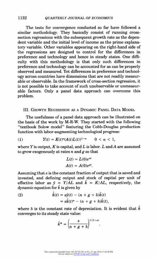
The usefulness of a panel data approach can be illustrated on the basis of the work by M-R-W. They started with the following "textbook Solow model" featuring the Cobb-Douglas production function with labor-augmenting technological progress:
(1) Y(t) = K(t)0(A(t)L(t))1-a 0 < a < 1,
where Y is output, K is capital, and L is labor. L and A are assumed to grow exogenously at rates n and g so that
L(t) = L(O)ent
A(t) = A(0)egt.
Assuming that s is the constant fraction of output that is saved and invested, and defining output and stock of capital per unit of effective labor as 9 = YIAL and k = K/AL, respectively, the dynamic equation for k is given by
(2) k(t) = s9(t) - (n + g + 6)k(t)
= sk(t)a - (n + g + 6)k(t),
where 8 is the constant rate of depreciation. It is evident that k converges to its steady state value:
k*= +
This content downloaded from 143.107.92.181 on Fri, 25 Apr 2014 17:43:38 PMAll use subject to JSTOR Terms and Conditions
GROWTH EMPIRICS: A PANEL DATA APPROACH 1133
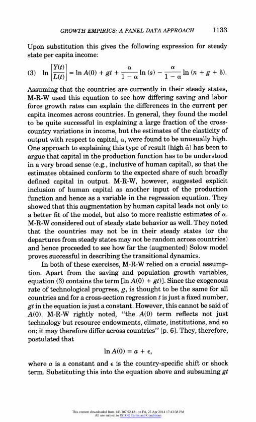
Upon substitution this gives the following expression for steady state per capita income:
Y(t) 1 a (3) in = I lnA(O) + gt + In (s) - In (n + g +
Assuming that the countries are currently in their steady states, M-R-W used this equation to see how differing saving and labor force growth rates can explain the differences in the current per capita incomes across countries. In general, they found the model to be quite successful in explaining a large fraction of the cross- country variations in income, but the estimates of the elasticity of output with respect to capital, a, were found to be unusually high. One approach to explaining this type of result (high a) has been to argue that capital in the production function has to be understood in a very broad sense (e.g., inclusive of human capital), so that the estimates obtained conform to the expected share of such broadly defined capital in output. M-R-W, however, suggested explicit inclusion of human capital as another input of the production function and hence as a variable in the regression equation. They showed that this augmentation by human capital leads not only to a better fit of the model, but also to more realistic estimates of a. M-R-W considered out of steady state behavior as well. They noted that the countries may not be in their steady states (or the departures from steady states may not be random across countries) and hence proceeded to see how far the (augmented) Solow model proves successful in describing the transitional dynamics.
In both of these exercises, M-R-W relied on a crucial assump- tion. Apart from the saving and population growth variables, equation (3) contains the term [ln A(O) + gt)]. Since the exogenous rate of technological progress, g, is thought to be the same for all countries and for a cross-section regression t is just a fixed number, gt in the equation is just a constant. However, this cannot be said of A(O). M-R-W rightly noted, "the A(O) term reflects not just technology but resource endowments, climate, institutions, and so on; it may therefore differ across countries" [p. 6]. They, therefore, postulated that
lnA(O) = a + E,
where a is a constant and e is the country-specific shift or shock term. Substituting this into the equation above and subsuming gt
This content downloaded from 143.107.92.181 on Fri, 25 Apr 2014 17:43:38 PMAll use subject to JSTOR Terms and Conditions
1134 QUARTERLY JOURNAL OF ECONOMICS
into the constant term a, they derived the specification:
My aa
(4) In \L=a + 1 _ In (s 1-( In (n +g + 8) + e.
At this stage, however, M-R-W made the assumption that E is independent of the explanatory variables, s and n. This was their identifying assumption, and this allowed them to proceed with the Ordinary Least Squares (OLS) estimation of the equation. M-R-W provided several arguments for this assumption. The first is that this assumption is common and is made not only in the Solow model, but also in other growth models. Also, they noted that in models where saving and population growth are endogenous but preferences are isoelastic, s and n are independent of E. Second, this identifying assumption renders it possible to test various informal hypotheses that have been made (proceeding from different growth theories) regarding the relationship between income, saving, and population growth. Third, since the specification above postulates not only the signs of the coefficients but also their proximate magnitudes, the regression results will allow testing of the joint hypothesis of validity of the Solow model and the above-mentioned identifying assumption.
Of these arguments the most important one is the first. However, the assumption of isoelastic preference represents an additional restriction. In general, the country-specific technology shift term E is likely to be correlated with the saving and population growth rates experienced by that country. At a heuristic level, since A(O) is defined not only in the narrow sense of production technology, but also to include resource endowments, institutions, etc., it is not entirely convincing to argue that saving and fertility behavior will not be affected by all that is included in A(O).
What is important to note here is that in the framework of a single cross-section regression, this assumption of independence becomes an econometric necessity. OLS estimation is valid only under this assumption. The other possibility in this regard is to recognize the correlation and then opt for instrumental variable (IV) estimation. However, given the nature and scope of the A(O) term, it is difficult to come up with instruments that will be correlated with the included explanatory variables of the model and yet uncorrelated with A(O). This makes the option of instrumental variable estimation not quite feasible.
Our basic conjecture is that a panel data framework provides a better and more natural setting to control for this technology shift
This content downloaded from 143.107.92.181 on Fri, 25 Apr 2014 17:43:38 PMAll use subject to JSTOR Terms and Conditions
GROWTH EMPIRICS: A PANEL DATA APPROACH 1135
term E. This is better revealed by considering the equation describ- ing out of steady state behavior. The way this equation is derived is as follows. Let 9* be the steady state level of income per effective worker, and let 9(t) be its actual value at any time t. Approximating around the steady state, the pace of convergence is given by
dIn 9(t) (5) dt- X[ln (9*)-In 9(t)],
dt
where A = (n + g + 8)(1 - oa). This equation implies that
(6) In9(t2) = (1 - e-AT) In9* + e-AT In9(t1),
where 9(t1) is income per effective worker at some initial point of time and T = (t2 - t1). Subtracting In 9(t1) from both sides yields
(7) 1n9(t2) - In9(t1) = (1 - e-At) In 9* - (1 - e-AT) In 9(t1).
This equation represents a partial adjustment process that be- comes more apparent from the following rearrangement:
(8) In9(t2) - In 9(t1) = (1 - e- XT)(In 9* - In9(t1)).
In the standard partial adjustment model, the "optimal" or "target" value of the dependent variable is determined by the explanatory variables of the current period. In the present case, 9* is determined by s and n, which are assumed to be constant for the entire intervening time period between t1 and t2 and hence represent the values for the current year as well. Substituting for 9* gives
(9) 1n9(t2) - In 9(t1) = (1 - e -AT) In (s) 1-(x
-(1 e XT) ln (n +g+5) - (1 -e-XT)ln9(tl).
M-R-W used this equation to study the process of convergence across different samples of countries. In their treatment t1 was 1960, and t2 was 1985. They assumed (g + 8) to be the same for all countries and equal to 0.05. The saving and population growth rates, s and n, were taken to be equal to the respective averages over 1960-1985.
The issue of correlation between the unobservable A(0) and the observed included variables is not apparent in equation (9) because it has been formulated in terms of income per effective worker. In actual implementation, however, M-R-W worked with
This content downloaded from 143.107.92.181 on Fri, 25 Apr 2014 17:43:38 PMAll use subject to JSTOR Terms and Conditions
1136 QUARTERLY JOURNAL OF ECONOMICS
income per capita. We may, therefore, reformulate the equation in terms of income per capita. Note that income per effective labor is
Y(t) Y(t) 9(t) = A(t)L(t) L(t)A(t)egt
so that
IY(t)\ In9(t) = In I I - In A(O) - gt \ L(t)/
= In y(t) - In A(O) - gt,
where y(t) is the per capita income, [Y(t)/L(t)]. Substituting for 9(t) into equation (9), we get the usual "growth-initial level" equation:
a (10) Iny(t2) - Iny(t1) = (1 - e-T) I_ n (s)
-(1 - e-AT) l In (n + g + ) -(1 - e-AT) lny(t1)
+ (1 - e AT) In A(O) + g(t2 -e -Tt)
However, if we collect terms with In y(t1) on the right-hand side, we get the equation in the following alternative form:
a (11) lny(t2) = (1 - e-AT) 1 ln (s)
- (1 - e-AT) aIn(n +g + 8) + e -Tlny(t1)
+ (1 - e AT) In A(O) + g(t2 -e -Ttl
It can now be seen that the above represents a dynamic panel data model with (1 - e -T) In A(O) as the time-invariant individual country-effect term. We may use the following conventional nota- tion of the panel data literature:
2
(12) Yit = YYit-i + E jijxI't + nt + pi + vit, j=1
where
yit= lny(t2)
yist-l = lny(t1) y = e-XT
This content downloaded from 143.107.92.181 on Fri, 25 Apr 2014 17:43:38 PMAll use subject to JSTOR Terms and Conditions
GROWTH EMPIRICS: A PANEL DATA APPROACH 1137
e~ -( -XeT)
I2 = -(1 - e-AT) 1-
il = In (s)
x2= In (n + g +)
ki = (1 - e-AT) In A(0)
It = g(t2 - XTt )I
and vit is the transitory error term that varies across countries and time periods and has mean equal to zero. Panel data estimation of this equation now provides the kind of environment necessary to control for the individual country effect.
It is clear that this panel data formulation is obtained by moving from a single cross-section spanning the entire period (1960-1985) to cross sections for the several shorter periods that constitute it. We may note that equation (11) was based on approximation around the steady state and was supposed to capture the dynamics toward the steady state. It is, therefore, valid for shorter periods as well. Also, it may be noted that in the single cross-section regression, s and n are assumed to be constant for the entire period. Such an approximation is more realistic over shorter periods of time. The panel data setup allows us, after controlling for the individual country effects, to integrate this process of convergence occurring over several consecutive time intervals. If we think that the character of the process of getting near to the steady state remains essentially unchanged over the period as a whole, then considering that process in consecutive shorter time spans should reflect the same dynamics. However, controlling for the unobservable individual country effects will create a cleaner canvas for the relationship among the measurable and included economic variables to emerge.
IV. ESTIMATION ISSUES AND DATA
A. Relevant Issues of Panel Estimation
A host of methods is available for the estimation of panel data models with individual effects.1 One common issue that arises in
1. For a recent review see Islam [1991].
This content downloaded from 143.107.92.181 on Fri, 25 Apr 2014 17:43:38 PMAll use subject to JSTOR Terms and Conditions
1138 QUARTERLY JOURNAL OF ECONOMICS
such estimation is whether the individual effects are to be thought of as "fixed" or "random." In the latter case the effects are assumed to be uncorrelated with the exogenous variables included in the model. In our case it is clear that estimators relying on such assumptions (for example, GLS in Maddala [1971]) are not suitable because it is precisely the fact of correlation that forms the basis of our argumentation for the panel approach.
The Least Squares with Dummy Variables (LSDV) estimator which is based on the fixed-effects assumption is still permissible, although that assumption may seem too strong. One problem with LSDV for our model, however, arises from its dynamic character. The presence of a lagged dependent variable on the right-hand side of equation (12) makes LSDV an inconsistent estimator, when asymptotics are considered in the direction of N -> oo. However, the asymptotic properties of panel data estimators can be considered in the direction of T, and Amemiya [1967] has shown that when considered in that direction, LSDV proves to be consistent and asymptotically equivalent to the Maximum Likelihood Estimator (MLE). Yet many other estimators start by eliminating the indi- vidual-effect term through first differencing. For these estimators, therefore, it does not matter whether the effect is fixed or random, and in the latter case, whether correlated or not.
The theoretical properties of most of these estimators are asymptotic, and in terms of these properties they are equivalent. In order to decide which of these to use, we conducted a Monte Carlo study based on the data set used in this paper and closely calibrated to the parameter values obtained from preliminary estimation. These results show that the LSDV estimator, although consistent in the direction of T only, actually performs very well. The other estimator that showed better performance is the Minimum Dis- tance (MD) estimator proposed by Chamberlain [1982, 1983].2 This estimator is specially designed for models where the individual effects are correlated with the included exogenous variables. The MD estimator has the added attractive property that it is robust to any presence of serial correlation in the vit term. In the following we present the results from both LSDV and MD estimation. It is reassuring that the results are very similar to each other.
B. Data and Samples
One of the reasons for the recent surge in work on growth empirics has been the availability of the Summers-Heston [1988]
2. Details of these results can be seen in Islam [1992].
This content downloaded from 143.107.92.181 on Fri, 25 Apr 2014 17:43:38 PMAll use subject to JSTOR Terms and Conditions

GROWTH EMPIRICS: A PANEL DATA APPROACH 1139
data set. In fact, the emergence of new (endogenous) growth theories can be traced to some of the empirical regularities of cross-country growth which this data set helped to bring to the fore and which at first sight seemed to contradict the implications of the existing neoclassical growth models. It is interesting to note that the Summers-Heston data set also makes a panel approach to growth empirics possible because it includes various measures of the GDP and its components for different countries over several decades. Both Barro [1989] and M-R-W used the Summers-Heston data set to construct the variables. Our present exercise is also based on this data set.
Since we want to compare our panel results with, in particular, those obtained by M-R-W from their single cross-section regres- sions, we keep the country samples similar to those used by them. The three samples that M-R-W considered were (i) NONOIL (98 countries), (ii) INTER (75 countries), and (iii) OECD (22 coun- tries). However, data for some of the initial years on Indonesia and Burkina Faso are not available in the Summers-Heston data set. We therefore excluded these two countries from our samples. This led to our NONOIL sample having 96 countries, while the INTER sample has 74 countries. The size of the OECD sample remains the same.
The other respect in which our variable construction differs from that of M-R-W is in the treatment of the population growth variable n. M-R-W took n as the rate of growth of the working age population. In view of the difficulty of getting panel data on working age population, we depend on the population growth rates computed from the total population figures available in the Sum- mers-Heston data set. However, following M-R-W, we take (g + 6) to be equal to 0.05 and assume this value to be the same for all countries and all years.
The switch from a single cross section to a panel framework is made possible by dividing the total period into several shorter time spans. The question that arises is what is the appropriate length of such time spans. The furthest that one can go in this regard is to consider a time span of just one year (which is technically feasible given that the underlying data set provides annual data). For several reasons, however, it seems that yearly time spans are too short to be appropriate for studying growth convergence. Short- term disturbances may loom large in such brief time spans. Instead, we opt for five-year time intervals. Thus, considering the period 1960-1985, we have five data (time) points for each country: 1985, 1980, 1975, 1970, and 1965. When t = 1965, for example, t -
This content downloaded from 143.107.92.181 on Fri, 25 Apr 2014 17:43:38 PMAll use subject to JSTOR Terms and Conditions
1140 QUARTERLY JOURNAL OF ECONOMICS
1 is 1960, and saving and population growth variables are averages over 1960-1965. With this setup, the vi,'s are now five calendar years apart (alternatively, pertain to five-year spans) and hence may be thought to be less influenced by business cycle fluctuations and less likely to be serially correlated than they would be in a yearly data setup.
V. ESTIMATION RESULTS
A. Single Cross-Section Results
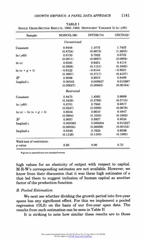
In order to see how much our results differ from those of M-R-W because of differences in samples and construction of variables, we first run single cross-section regressions analogous to those conducted by M-R-W. For these regressions Yit is the log of per capita GDP for 1985 and yit-1, the same for 1960. s and n are averages of saving and population growth rates for the period 1960-1985. The results can be seen in Table I. The first panel of the table gives results of estimation in unrestricted form, while the second panel contains results from estimation of the equation after imposing the restriction that the coefficients of the investment and population growth variables are equal in magnitude but opposite in sign. M-R-W's results (their Table IV) on this regression are available only in the unrestricted form. We can therefore compare the unrestricted results only.
Such a comparison shows that the results are very similar. The coefficients of the initial GDP and saving variable are very close to each other in the two tables. Modified for the difference in the way the equation is specified, our estimates of the initial GDP variable for NONOIL, INTER, and OECD samples will be -0.127, -0.218 and -0.328, respectively. Corresponding estimates of M-R-W are -0.141, -0.228, and 0.351, respectively. This is also reflected in the respective implied values of the rate of convergence parameter X. Our values of 0.00542, 0.0098, and 0.0 159 for NONOIL, INTER, and OECD are very close to the corresponding M-R-W estimates, namely, 0.00606, 0.0104, and 0.0173, respectively.
The results from restricted estimation allow us to get unique estimates of not only X, but also the output elasticity parameter, a. The estimates of X obtained from restricted estimation are almost the same as those from unrestricted estimation. In general, they confirm the finding of a very slow rate of convergence. On the other hand, the estimate of a is found to be 0.83 for the NONOIL sample, 0.76 for INTER, and 0.60 for OECD. These are, indeed, unusually
This content downloaded from 143.107.92.181 on Fri, 25 Apr 2014 17:43:38 PMAll use subject to JSTOR Terms and Conditions
GROWTH EMPIRICS: A PANEL DATA APPROACH 1141
TABLE I SINGLE CROSS-SECTION RESULTS, 1960-1985: DEPENDENT VARIABLE Is In (y85)
Sample: NONOIL(96) INTER(74) OECD(22)
Unrestricted
Constant 0.9448 1.1075 1.7433 (0.8724) (0.8975) (1.2655)
In (Y60) 0.8733 0.7822 0.6722
(0.0611) (0.0667) (0.0694)
In (s) 0.6585 0.6431 0.4114
(0.0926) (0.1121) (0.1845)
In (n + g + 5) -0.6122 -0.8144 -0.8021 (0.3667) (0.3717) (0.4187)
R 0.9006 0.8915 0.8499
ImpliedX 0.00542 0.009827 0.015887
(0.00037) (0.00083) (0.00164)
Restricted
Constant 0.8475 1.4565 2.6689 (0.3429) (0.3798) (0.5715)
In (Y60) 0.8701 0.7945 0.6817
(0.0547) (0.0599) (0.0678)
In (s) - In (n + g + 5) 0.6554 0.6610 0.4847 (0.0884) (0.1034) (0.1602)
R 0.9037 0.8927 0.8524
Implied X 0.005565 0.009204 0.015327
(0.00035) (0.00069) (0.00152)
Implied a 0.8346 0.7628 0.6036
(0.1126) (0.1193) (0.1995)
Wald test of restriction: p-value 0.95 0.90 0.70
Figures in parentheses are standard errors.
high values for an elasticity of output with respect to capital. M-R-W's corresponding estimates are not available. However, we know from their discussion that it was these high estimates of a that led them to suggest inclusion of human capital as another factor of the production function.
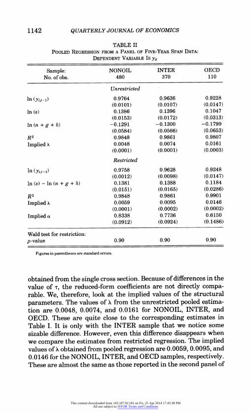
B. Pooled Estimation
We next see whether dividing the growth period into five-year spans has any significant effect. For this we implement a pooled regression (OLS) on the basis of our five-year span data. The results from such estimation can be seen in Table II.
It is striking to note how similar these results are to those
This content downloaded from 143.107.92.181 on Fri, 25 Apr 2014 17:43:38 PMAll use subject to JSTOR Terms and Conditions
1142 QUARTERLY JOURNAL OF ECONOMICS
TABLE II POOLED REGRESSION FROM A PANEL OF FIvE-YEAR SPAN DATA:
DEPENDENT VARIABLE Is Yit
Sample: NONOIL INTER OECD No. of obs. 480 370 110
Unrestricted
in (yi,t-i) 0.9764 0.9636 0.9228 (0.0101) (0.0107) (0.0147)
in (s) 0.1386 0.1396 0.1047 (0.0153) (0.0172) (0.0313)
in (n + g + 5) -0.1291 -0.1300 -0.1799 (0.0584) (0.0566) (0.0653)
R2 0.9848 0.9861 0.9807
Implied X 0.0048 0.0074 0.0161 (0.0001) (0.0001) (0.0003)
Restricted
in (yi,t-1) 0.9758 0.9628 0.9248 (0.0012) (0.0098) (0.0147)
in (s)-in (n + g + 5) 0.1381 0.1388 0.1184 (0.0151) (0.0165) (0.0286)
R2 0.9848 0.9861 0.9901 Implied X 0.0059 0.0095 0.0146
(0.0001) (0.0002) (0.0002) Implied a 0.8338 0.7736 0.6150
(0.0912) (0.0924) (0.1486)
Wald test for restriction: p-value 0.90 0.90 0.90
Figures in parentheses are standard errors.
obtained from the single cross section. Because of differences in the value of T, the reduced-form coefficients are not directly compa- rable. We, therefore, look at the implied values of the structural parameters. The values of X from the unrestricted pooled estima- tion are 0.0048, 0.0074, and 0.0161 for NONOIL, INTER, and OECD. These are quite close to the corresponding estimates in Table I. It is only with the INTER sample that we notice some sizable difference. However, even this difference disappears when we compare the estimates from restricted regression. The implied values of . obtained from pooled regression are 0.0059, 0.0095, and 0.0146 for the NONOIL, INTER, and OECD samples, respectively. These are almost the same as those reported in the second panel of
This content downloaded from 143.107.92.181 on Fri, 25 Apr 2014 17:43:38 PMAll use subject to JSTOR Terms and Conditions
GROWTH EMPIRICS: A PANEL DATA APPROACH 1143
Table I. The implied values of a obtained from these two regres- sions are also found to be strikingly similar.
These results, therefore, show that dividing the period into shorter spans and considering the growth process over shorter consecutive intervals does not affect the results. Both the single cross section and the pooled regression produce very similar results. We find very low estimates of the rate of convergence (particularly for the NONOIL and INTER samples) and very high estimates of the elasticity parameter a. We next see how panel estimation changes these results.
C. Minimum Distance: Estimation with "Correlated Effects"
The MD estimator emphasizes the correlated nature of the individual-effect term and does not eliminate it by differencing the equation. Instead, it attempts to incorporate the correlation in the estimation process by explicitly specifying kLi as a function of the variables with which it is thought to be correlated.
One simple specification of kLi suggested by Mundlak [1978] is to take it as a function of the mean of the exogenous variable pertaining to the individual, xi (assuming that we have only one exogenous variable, xit, in the model and 3 is its coefficient). Mundlak's purpose in using such a simple specification was, however, to show that if kLi is a linear function of x-i, then the GLS estimation under the random effects assumption reduces to the LSDV estimation under the fixed effects assumption.
Chamberlain noted that the specification of ,i suggested by Mundlak was overly restrictive. He, therefore, proposed a more general specification whereby kLi depends linearly on the xi for all time periods. Thus, we would have
(13) ,ui = Ko + K1Xij + K2Xi2 + + KTXiT + PJi
with E [i lxi,, . . ., XiT] = 0. Note that, regarded as a linear predictor, the above specification does not entail any restriction. This then allows substitution for kLi in equation (12) by its specification in terms of xit's as given by equation (13). Also, by repeated substitution we can replace the lagged dependent variable on the right-hand side by expressions involvingyi0, the initial value. Instead of assuming the yiO's as given and fixed, Chamberlain suggested a similar general specification for yi in terms of xit's:
(14) Yio = No + (lXil + (2Xj2 + ... + (TXiT + Pi,
This content downloaded from 143.107.92.181 on Fri, 25 Apr 2014 17:43:38 PMAll use subject to JSTOR Terms and Conditions
1144 QUARTERLY JOURNAL OF ECONOMICS
where, again, E[Rjlxij.... , XiT1] - 0. Note that, interpreted as linear predictor, the above specification is perfectly general. We can then substitute equation (14) for Yio in equation (12). Through these substitutions we arrive at a system of reduced-form equa- tions, all of which have only the xi,'s as the right-hand side variables. Estimation of these reduced-form equations gives us the HI-matrix of the reduced-form coefficients. Structural parameters are then obtained by imposing the nonlinear constraints on the IH-matrix through the MD procedure. A brief discussion of this estimation procedure has been provided in Appendix 4.
We implement the MD estimation procedure for the equation in the restricted form. Hence the equation is
(15) YU = Yist-l + exit + mt + ki + Vit,
where
ax = (1 - e-XT)
xit = In (s) - In (n + g + a).
The rest of the notation is as in equation (12). Since the MD results showed some sensitivity to the starting values of the iteration process, we conducted a sensitivity analysis based on the MD statistic and obtained results that yielded the minimum value of this statistic for different alternative combinations of the starting values for -y and P. In other words, we tried to achieve the global minimum instead of a local one. However, it needs to be mentioned that due to small N, the MD estimates for the OECD sample may be less accurate than for the other two samples.3
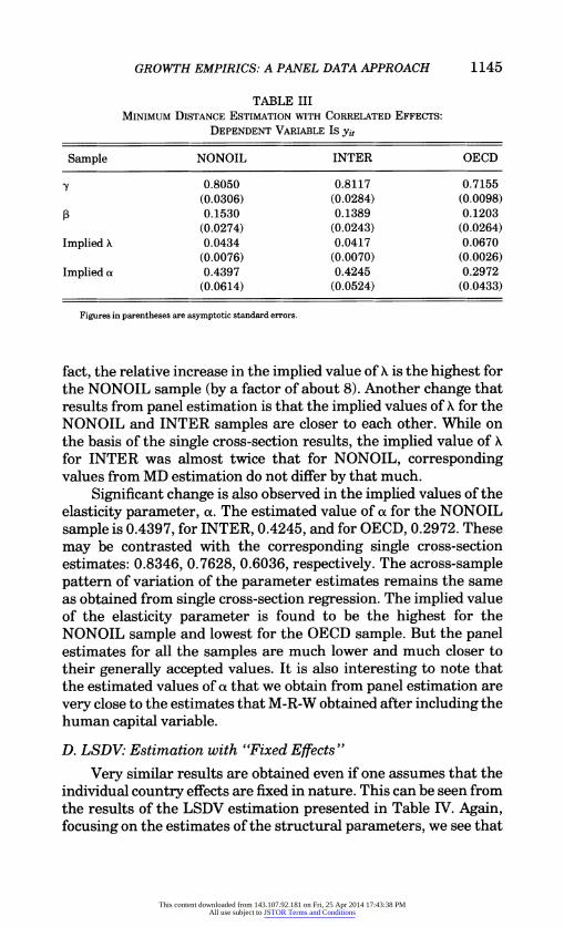
The results from MD estimation can be seen in Table III. For reasons stated earlier, we again focus on the estimated values of the structural parameters only. It is clear from Table III that panel estimation allowing for correlated individual country effects leads to considerable change in the results. The implied value of X from the MD estimation for the NONOIL sample is 0.0434, for INTER it is 0.0456, and for OECD, 0.0670. These are indeed much higher values than the corresponding single cross-section values. The rate of convergence obtained for the OECD sample still remains much higher than that found for either the NONOIL or INTER samples, but even for these latter samples it is now appreciably higher. In
3. The weighting matrix becomes nearly singular, and sensitivity analysis with respect to the initial values for the parameter ,3 remains less than conclusive.
This content downloaded from 143.107.92.181 on Fri, 25 Apr 2014 17:43:38 PMAll use subject to JSTOR Terms and Conditions
GROWTH EMPIRICS: A PANEL DATA APPROACH 1145
TABLE III MINIMUM DISTANCE ESTIMATION WITH CORRELATED EFFECTS:
DEPENDENT VARIABLE IS yit
Sample NONOIL INTER OECD
y 0.8050 0.8117 0.7155 (0.0306) (0.0284) (0.0098)
0 0.1530 0.1389 0.1203 (0.0274) (0.0243) (0.0264)
Implied X 0.0434 0.0417 0.0670 (0.0076) (0.0070) (0.0026)
Implied at 0.4397 0.4245 0.2972 (0.0614) (0.0524) (0.0433)
Figures in parentheses are asymptotic standard errors.
fact, the relative increase in the implied value of A is the highest for the NONOIL sample (by a factor of about 8). Another change that results from panel estimation is that the implied values of X for the NONOIL and INTER samples are closer to each other. While on the basis of the single cross-section results, the implied value of A for INTER was almost twice that for NONOIL, corresponding values from MD estimation do not differ by that much.
Significant change is also observed in the implied values of the elasticity parameter, at. The estimated value of a for the NONOIL sample is 0.4397, for INTER, 0.4245, and for OECD, 0.2972. These may be contrasted with the corresponding single cross-section estimates: 0.8346, 0.7628, 0.6036, respectively. The across-sample pattern of variation of the parameter estimates remains the same as obtained from single cross-section regression. The implied value of the elasticity parameter is found to be the highest for the NONOIL sample and lowest for the OECD sample. But the panel estimates for all the samples are much lower and much closer to their generally accepted values. It is also interesting to note that the estimated values of a that we obtain from panel estimation are very close to the estimates that M-R-W obtained after including the human capital variable.
D. LSDV: Estimation with "Fixed Effects"
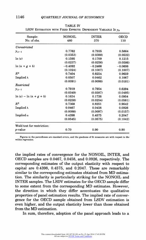
Very similar results are obtained even if one assumes that the individual country effects are fixed in nature. This can be seen from the results of the LSDV estimation presented in Table IV. Again, focusing on the estimates of the structural parameters, we see that
This content downloaded from 143.107.92.181 on Fri, 25 Apr 2014 17:43:38 PMAll use subject to JSTOR Terms and Conditions
1146 QUARTERLY JOURNAL OF ECONOMICS
TABLE IV LSDV ESTIMATION WITH FIXED EFFECTS: DEPENDENT VARIABLE Is Yit
Sample: NONOIL INTER OECD No. of obs. 480 370 110
Unrestricted Yit-1 0.7762 0.7935 0.5864
(0.0353) (0.0388) (0.0532) In (s) 0.1595 0.1709 0.1215
(0.0237) (0.0256) (0.0586) In (n + g + 8) -0.4092 -0.2466 -0.0698
(0.1024) (0.1007) (0.1007) R2 0.7404 0.8254 0.9659 ImpliedX 0.0507 0.0462 0.1067
(0.0091) (0.0098) (0.0181) Restricted Yit-1 0.7919 0.7954 0.6294
(0.0349) (0.0387) (0.0495) In (s) - In (n + g + 8) 0.1634 0.1726 0.0954
(0.0238) (0.0254) (0.0581) R2 0.7368 0.8251 0.9642 ImpliedX 0.0467 0.0458 0.0926
(0.0088) (0.0097) (0.0157) Implied a 0.4398 0.4575 0.2047
(0.0545) (0.0575) (0.1042)
Wald test for restriction: p-value 0.70 0.90 0.90
Figures in the parentheses are standard errors, and the goodness of fit measures are with respect to the within regression.
the implied rates of convergence for the NONOIL, INTER, and OECD samples are 0.0467, 0.0458, and 0.0926, respectively. The corresponding estimates of the output elasticity with respect to capital are 0.4398, 0.4575, and 0.2047. These are remarkably similar to the corresponding estimates obtained from MD estima- tion. The similarity is particularly striking for the NONOIL and INTER samples. The LSDV estimates for the OECD sample differ to some extent from the corresponding MD estimates. However, the direction in which they differ accentuates the qualitative properties of panel estimation results. The implied rate of conver- gence for the OECD sample obtained from LSDV estimation is even higher, and the output elasticity lower than those obtained from the MD estimation.
In sum, therefore, adoption of the panel approach leads to a
This content downloaded from 143.107.92.181 on Fri, 25 Apr 2014 17:43:38 PMAll use subject to JSTOR Terms and Conditions
GROWTH EMPIRICS: A PANEL DATA APPROACH 1147
twofold change in the results. First, we obtain much higher rates of convergence, and second, we obtain more empirically plausible estimates of the elasticity of output with respect to capital. In the section below we try to consider the source and implications of each of these results.
VI. INTERPRETATION OF THE RESULTS
A. Statistical Interpretation
The statistical source of the change in the parameter estimates is not very difficult to comprehend. Both of the above-noted changes can, to a great extent, be attributed to correction for omitted variable bias that the panel approach makes possible.
We have seen in Section II that, in the framework of single cross-section regression, the A(O) term, being unobservable or unmeasurable, is left out of the equation (or, subsumed in the error term). This actually creates an omitted variable problem. Since this omitted variable is correlated with the included explanatory vari- ables, it causes the estimates of the coefficients of these variables to be biased. The direction of bias can be assessed from the standard formula for omitted variable bias. The partial correlation between A(O) and the initial value of y is likely to be positive, and the expected sign of the A(O) term in the full regression, as can be seen in equation (11), is also positive. Thus, 'y, the estimated coefficient ofyi t_1, is biased upward. The relationship between A and y is given by
(16) A = (1/X) In (,y).
This equation shows that a higher value of My leads to a lower value of X. This explains why we get lower convergence rates from single cross-section regressions and pooled regressions that ignore corre- lated individual country effects.
Similarly, the relationship between ax and the reduced-form coefficients y and 3 is
(17) a = /(1-+ 13).
This formula for a clearly shows that overestimation of y also leads to a higher implied value of at. Since 3 figures in both the numerator and the denominator, the net effect of any bias in the estimate of P on the value of a is not immediately clear. It depends on the range of values that this estimated coefficient takes. We
This content downloaded from 143.107.92.181 on Fri, 25 Apr 2014 17:43:38 PMAll use subject to JSTOR Terms and Conditions
1148 QUARTERLY JOURNAL OF ECONOMICS
have seen above what the likely effect on the estimate of y can be when the correlated individual country effect is ignored.
We may apply similar reasoning to assess the likely effect of ignoring the individual effect on the estimate of P. Recall that in the restricted form, P3 is the coefficient of [In (s) - In (n + g + 6)]. The theoretical sign of the coefficient is positive. However, it is difficult to be sure about the partial correlation of A(O) with [In (s) - In (n + g + 6)]. Whatever may be the direction of bias in the estimate of P3, because of its presence in both the numerator and the denominator, the effect of this bias may, to a large extent, cancel out, and bias (and its correction) in the estimate of y may be a determining factor. As equation (18) shows, a lower value of 'y leads to a lower value of a.
This is, obviously, the narrow statistical interpretation of our results. We next turn to the interpretation and implications of the results from growth theory's point of view.
B. Estimation Results and Growth Theory
In the growth literature of recent years, three empirical results have surfaced. These are (i) absence of absolute conver- gence among the countries in the larger sample, (ii) slow condi- tional convergence among countries in the larger sample, and (iii) absolute or faster conditional convergence among "similar" sub- groups of countries of the larger sample. As we have previously noted, it was the first finding (with or without the third) that triggered the development of new (endogenous) theories of growth. The concept of conditional convergence to some extent reinstated the "old" Solow-Cass-Koopmans theory of growth, although, so far, that needed incorporation of human capital into the model. However, even after accounting for human capital, growth empir- ics based on a single cross-section regression yielded a rather slow rate of conditional convergence, which is problematic, because an open economy version of the Solow-Cass-Koopmans model predicts instantaneous convergence.
It is in this context that we need to evaluate the panel estimation results that we have obtained. First of all, the finding of a faster rate of conditional convergence (even without taking account of human capital) is obviously good news for the Solow- Cass-Koopmans model. The rates of conditional convergence ob- tained from panel estimation are nowhere near infinity, but they are much higher than the corresponding rates obtained from single cross-section regressions and hence lend somewhat more validity
This content downloaded from 143.107.92.181 on Fri, 25 Apr 2014 17:43:38 PMAll use subject to JSTOR Terms and Conditions
GROWTH EMPIRICS: A PANEL DATA APPROACH 1149
to the cross-country implications of the Solow-Cass-Koopmans model.
Equation (3) shows that the steady state income levels differ across countries not only because of differences in s and n (and possibly because of differences in 8, and, in particular, g), but also because of differences in A(O). The question is whether differences in A(O) are important enough to have significant impact on cross-country growth regularities. If they were not important, holding these constant through the panel framework, would not make much difference in the results. The fact that it does shows that these differences indeed play an important role in understand- ing the international growth experience. In other words, the A(O) term is an important source of parametric difference in the aggregate production function across countries. The process of convergence is thwarted to a great extent by persistent differences in technology level and institutions.
This finding is consistent with the generic finding of faster convergence among groups of similar countries that have been reported earlier by researchers. Instead of adopting the panel data approach, the other way to control for differences in technology and institutions is to classify the countries into similar groups. Baumol [1986] coined the term "convergence club" to express this phenome- non. The classification itself can, however, be problematic. The way Baumol did it suffered from self-selection bias, as was demon- strated by De Long [1988]. Recently, Chua [1992] did an analysis where similar could be interpreted as geographic contiguity. Durlauf and Johnson [1991] attempted to endogenize the classification using the "regression tree" method. In all these cases, convergence was found to be much stronger within the groups and weak between them. Durlauf and Johnson were quite emphatic about the cause of this result. They concluded that the aggregate production function differed across different locally convergent groups and hence suggested that, ". . . the Solow growth model should be supplemented with a theory of aggregate production function differences in order to fully explain international growth patterns" [p. 1]. What we have done in this paper is, by adoption of a panel data approach, to allow for differences in the aggregate production function not only across groups of countries (however defined), but across individual countries. As a result, we obtain higher rates of convergence over the samples as a whole.
Having seen the impact of inclusion of individual country effects on growth regression results, we now turn to the question of
This content downloaded from 143.107.92.181 on Fri, 25 Apr 2014 17:43:38 PMAll use subject to JSTOR Terms and Conditions
1150 QUARTERLY JOURNAL OF ECONOMICS
what happens when human capital is brought into the panel framework of analysis.
VII. INCLUSION OF HUMAN CAPITAL
Measures of human capital have always been a weak spot in growth empirics. In fact, M-R-W provide a very good discussion of the problems and issues involved in this regard. We cannot use the identical SCHOOL variable in our analysis because analogous panel data on this variable are difficult to come by. Moreover, since M-R-Ws' work, Barro and Lee [1993] have made important progress in putting together a human capital data set for a wide cross section of countries. Based on census data and myriads of other informa- tion they have constructed a human capital variable, named HUMAN, which gives the average schooling years in the total population over age 25. While the SCHOOL variable is based on secondary schooling information only, HUMAN includes schooling at all levels, primary, secondary, and higher, complete and incom- plete. Second, HUMAN gives a direct measure of the stock of human capital, and hence makes it possible to estimate the equation in which human capital appears as a stock. The restricted form of this equation is
ax (18) lny(t2) = (1 - e-AT) 1 [In (s) - In (n + g + 8)]
+ (1 - eXT) In (h*) + e -T In y(tl)
+ (1 - e AT) In A(0) + g(t2 - eXTti)
where h* is the steady state level of human capital, and (p is the exponent of the human capital variable in the augmented produc- tion function of M-R-W.
Inclusion of the human capital variable in our analysis, however, requires some modification of the sample sizes. This is because the panel data on HUMAN in Barro and Lee [1993] are not available for all the countries of our original samples. Accordingly, the NONOIL sample now reduces to 79 countries,4 and INTER to 67.5 Size of the OECD sample, expectedly, remains unchanged.
4. The countries dropped from the original NONOIL sample are Angola, Benin, Burundi, Cameroon, Central African Republic, Chad, Congo, Egypt, Ethio- pia, Ivory Coast, Madagascar, Mali, Mauritania, Morocco, Nigeria, Rwanda, and Somalia.
5. The countries dropped from the original INTER sample are Cameroon, Ethiopia, Ivory Coast, Madagascar, Mali, Morocco, and Nigeria.
This content downloaded from 143.107.92.181 on Fri, 25 Apr 2014 17:43:38 PMAll use subject to JSTOR Terms and Conditions

GROWTH EMPIRICS: A PANEL DATA APPROACH 1151
TABLE V ESTIMATION WITH HUMAN CAPITAL
Single Pooled Panel Variable cross section regression estimation
NONOIL
ln(h) 0.1823 0.0093 -0.0712 (0.0895) (0.0146) (0.0323)
Implied X 0.0111 0.0069 0.0375 (0.0038) (0.0025) (0.0093)
Implied at 0.6862 0.8013 0.5224 (0.0694) (0.0534) (0.0642)
Implied up 0.2356 0.0544 -0.1990 (0.1013) (0.1020) (0.1097)
INTER
ln(h) 0.1101 -0.0014 -0.0027 (0.1305) (0.0209) (0.0471)
Implied X 0.0118 0.0079 0.0444 (0.0045) (0.0028) (0.0102)
Implied a 0.6906 0.7854 0.4947 (0.0799) (0.0587) (0.0599)
Implied up 0.1335 -0.0077 -0.0069 (0.1428) (0.1288) (0.1261)
OECD
ln(h) 0.0864 0.0034 -0.0208 (0.1551) (0.0268) (0.0449)
Implied X 0.0187 0.0162 0.0913 (0.0077) (0.0055) (0.0160)
Implied ax 0.5416 0.6016 0.2074 (0.1426) (0.1015) (0.1055)
Implied up 0.1062 0.0174 -0.0450 (0.2027) (0.1797) (0.1457)
Figures in parentheses are standard errors.
Before moving on to panel estimation, it is instructive to note the results obtained from inclusion of the human capital variable in the single cross-section and pooled regression frameworks.6 These have been presented along with results from panel estimation in Table V. Looking at the single cross-section results, we observe the following. First, in general, the outcome is similar in spirit to that found by M-R-W and other researchers. Inclusion of the human
6. We also check for the effect of the modification of the samples on estimation without human capital. These results are not presented here. In general, the sample modifications do not significantly change the results.
This content downloaded from 143.107.92.181 on Fri, 25 Apr 2014 17:43:38 PMAll use subject to JSTOR Terms and Conditions
1152 QUARTERLY JOURNAL OF ECONOMICS
capital variable in the single cross-section regression framework does lead to higher rates of convergence and lower values of at. In our case, however, the changes are of a lesser order.7 Second, judging by the size of the standard errors, the human capital variable does not prove to be significant for all the different samples. Even in M-R-W the SCHOOL variable did not prove to be significant for the OECD sample. In our case the same is found for the INTER sample as well. Third, while for the NONOIL sample the value of (p (0.2356), the implied exponent for the human capital variable, was found to be very similar to that found by M-R-W, for the INTER and OECD samples the estimates are substantially lower: 0.1335 and 0.1062, respectively, compared with 0.23 of M-R-W in both cases.
Turning to pooled estimation, we find that the results change in a very different direction. First of all, we note that the human capital variable now loses statistical significance for the NONOIL sample as well. Second, for the INTER sample it even assumes the wrong sign. Third, with respect to the impact on the implied values of X, the estimates now decrease to 0.0069, 0.0079, and 0.0162 for the NONOIL, INTER, and OECD samples, respectively. On the other hand, estimated values of ax increase to 0.8013, 0.7854, and 0.6016, respectively. These estimates are very similar to those obtained from single cross-section regression without the human capital variable. What this implies is that incorporation of the time dimension of the human capital variable into the analysis annihi- lates the effect that the cross-sectional variation in human capital had on the regression results. It is against this background that we now consider the results from panel estimation. These can be seen in the last column of Table V.
The figures in that column show that introduction of indi- vidual country effects reproduces the earlier result even in the presence of time series of human capital. The implied values of X are now found to be 0.0375, 0.0444, and 0.0913 for the NONOIL, INTER, and OECD samples, respectively. The implied values of ax are 0.5224, 0.4947, and 0.2074 for these samples, respectively. Note that these results are broadly similar to the panel results that
7. There may be several reasons for this. First, the samples are not the same. Second, the human capital variable used is not the same. Third, the form in which the human capital variable has been entered into the equation is different. Equation (19) requires a steady state level of human capital. In actual implementation we have used the HUMAN of the end points of time for the respective time spans. This is different from using either the initial measure of human capital (as in Barro [1989]) or the average for the period (as in M-R-W [1992]).
This content downloaded from 143.107.92.181 on Fri, 25 Apr 2014 17:43:38 PMAll use subject to JSTOR Terms and Conditions
GROWTH EMPIRICS: A PANEL DATA APPROACH 1153
we obtained earlier without including human capital. This is also not surprising in view of the fact that the human capital variable does not prove to be significant for two of the three samples. Also of note is the fact that in all three samples, the coefficient on the human capital variable now appears (in the restricted version of the model) with the wrong sign. In the case of the INTER sample, the magnitude of the coefficient and the implied value of .p are negligible. To a great extent, the same is true for OECD sample. It is only for the NONOIL sample that we find the negative coefficient on the human capital to be sizable and marginally significant.
However, such "anomalous" results regarding the role of human capital in the growth process are not new. Whenever researchers have attempted to incorporate the temporal dimension of human capital variables into growth regressions, outcomes of either statistical insignificance or negative sign have surfaced.8 So far, there have been two kinds of responses to these types of results. One is to point out the discrepancy between the theoretical variable H in the production function and the actual variable used in regressions. The enrollment rates were always very partial measures of the rate of investment in human capital and, more importantly, did not account for differences in the quality of schooling. Although, measured by such rates, many (particularly the less developed) countries appear to have made much progress, the true levels of human capital (and hence the output levels) in these countries have actually not increased by that much. Statisti- cally this results in a negative temporal relationship between the human capital variable used and economic growth within coun- tries. The results of the pooled regression already show that this negative temporal relationship is strong enough to outweigh the positive cross-sectional relationship. Since panel estimators rely more on "within" variation, we find that in panel results the negative temporal relationship surfaces more forcefully. From this point of view, what our results show is that even Barro and Lee's HUMAN variable, though much more comprehensive in its scope, is nonetheless not free from the above issue of discrepancy. Also, in light of the above, it is no wonder that it is in the NONOIL sample that the negative effect of the HUMAN variable is found to be more pronounced.
The second response is to think of richer specification of the production function with respect to human capital. In a sense,
8. For one such example see De Gregorio [1991].
This content downloaded from 143.107.92.181 on Fri, 25 Apr 2014 17:43:38 PMAll use subject to JSTOR Terms and Conditions

1154 QUARTERLY JOURNAL OF ECONOMICS
Romer [1989b] can be thought of as a pioneer in this regard. The recent work by Benhabib and Spiegel [1994] is another significant step in this direction. Their estimation of a growth equation in the first differenced form (which may be regarded as panel estimation with two periods only), results in insignificant or negative coeffi- cients on the human capital variable for all different samples and in all different versions.9 This led them to propose a more complex specification involving interaction between A(t), H, g, and also the gap between the individual country's level of A(t) and that of the leading country. Such a specification opens up multiple channels for the human capital variable to have impact on growth, which then allows the theoretical properties of the human capital variable to be better reflected in the regression results. While the issue of inadequacy of the currently available variables as measures of human capital across countries cannot be belittled, the approach taken by Benhabib and Spiegel and others is certainly more promising. The analysis in the next section indeed shows that human capital is closely related to the estimated values of the A(O) term. Benhabib and Spiegel, however, limit their analysis to single cross-section regression with some variables entering in the first differenced form. We intend to extend this approach to the panel framework in a future paper. Empirical work has so far clearly established that human capital plays a very important role in the growth process. However, the question that remains still unre- solved is, In What Exact Way?
In sum, therefore, the above exercise shows that, despite the pitfalls encountered regarding the role of human capital, the effect of controlling for the differences in the A(O) term remains robust. The main properties of the panel results remain unchanged whether or not we include human capital in the regression.
VIII. ESTIMATED COUNTRY EFFECTS: A TENTATIVE ANALYSIS
Panel estimation permits us not only to allow for the indi- vidual country effects in the estimation of the other parameters of the model, but also to get the estimates of these effects themselves. In the case of LSDV estimation the recovery of the estimated
9. As they reported, ". . . the coefficient for human capital is insignificant and enters with the wrong sign. . . . this result is independent of whether we use the Kyriacou, Barro-Lee, or literacy data sets as proxies for the stock of human capital in computing the growth rates of human capital" [Benhabib and Spiegel 1994, p. 154].
This content downloaded from 143.107.92.181 on Fri, 25 Apr 2014 17:43:38 PMAll use subject to JSTOR Terms and Conditions
GROWTH EMPIRICS: A PANEL DATA APPROACH 1155
individual effects is direct because they are the estimated coeffi- cients of the country dummies. If LSDV is implemented in the form of "within-regression"-as we do-the estimated country effects are obtained as
(19) pi =i - - P3Xi - 9,
where
l T 1 T-1 T T
i= T KiY Yi,-1 = X = I I
with t being the estimates of the time effects. In the case of the correlated effects model, the MD estimation procedure yields estimates of Kt. These can now be substituted back into equation (14) to get the estimated country effects.
The estimated values of ,ui's are presented in column 3 of Appendix 1.10 The implied values of In A(O)i can be recovered from the 'ii's using the formula, ki = (1 - e-XT) lnA(O)i. These are presented in column 4. The dispersion and relative position of the countries can be highlighted by computing the values of A(O)i and expressing them relative to A(O)min (in the present case, the A(0) of Somalia). These ratios may be called the A(0) index, and they are presented in column 5. The rank of the countries in terms of this index can be seen in column 6. The value of the index ranges from 1 to about 40, showing that the countries do vary enormously in terms of their A(O) values. In general, however, we find a bottom- heavy distribution. If we classify the countries according to whether the estimated A(0) index is less than 5, between 5 and 10, 10 and 15, 15 and 20, 20 and 25, and greater than 25, and name the corresponding groups for easy reference as I (Very Low), II (Low), III (Medium), IV (High), V (Very High), and VI (Super High), then we find that 63 (i.e., 66 percent) of the countries of the sample fall into the lowest two groups. The histogram in Appendix 2 gives a more visual display of the distribution along with Appendix other information that makes it easy to read off from it both the rank and the value of the A(0) index for particular countries.
The A(0) index is, obviously, a measure of efficiency with which the countries are transforming their capital and labor resources into output and hence is very close to the conventional
10. The estimates presented in Appendix 1 are based on NONOIL results. The relative rankings of the countries do not change when these country effects are estimated on the basis of the INTER sample. Also, the MD and LSDV yield similar estimates when rounded up to two decimal points.
This content downloaded from 143.107.92.181 on Fri, 25 Apr 2014 17:43:38 PMAll use subject to JSTOR Terms and Conditions
1156 QUARTERLY JOURNAL OF ECONOMICS
concept of total factor productivity (TFP). The important differ- ence is that while the TFPs are computed for the individual countries on the basis of their respective time series data, the country effects are inherently based on cross-country comparison and are not subsequent upon individual country-analysis.
Appendix 3 gives a two-way distribution of the countries in terms of the A(O) index and continents. In general, it conforms to what may be called the expected pattern. A large proportion (84 percent) of the African countries fall in the Very Low group. On the other hand, most of the European countries are in the High and Very High groups. Latin and Central American countries generally tend to avoid the Very Low group, and instead belong mostly (about half) to Group II. The Asian countries seem to be more widely distributed across the groups. While a good number of them (about one-third) fall into the Very Low group, many of the rest make their way to the higher groups.
In recent years there has been renewed interest in in-depth analysis of growth performance of individual countries (see, for example, Young [1992, 1995]). In light of this interest, it may be worthwhile to note certain "unexpected" or interesting aspects of the results regarding the A(O) index. First is the super high value of this index for Hong Kong. Not only did it have the highest value, but it surpassed by this measure the next ranking country (Canada) by a wide margin. Hong Kong's super value of the A(O) index, compared with that of Singapore, lends support to some of Young's [1992] conclusions from his detailed analysis of the comparative growth performance of these two city states. Second, the high values of the A(O) index for the United States and Canada may to some extent dispel the thesis of productivity slowdown in these countries, in particular, the United States. This is further supported by the relatively low values of the A(O) index for both Japan and Germany. Third, some of the countries did remarkably well in terms of the A(O) index. Among these are, for example, Israel, Trinidad and Tobago, and Venezuela and also to some extent, Syria and South Africa.1" Fourth, equally noteworthy is the poor A(O) index of some other countries. Among the latter are, for example, Korea, Chile, Portugal, and India. This result, particu- larly regarding Korea and Chile, may draw some attention.
Having seen the range, dispersion, and ranking, we may next
11. However, it may be necessary to check into the possible role of extraction of oil and other mineral deposits in this regard, particularly with respect to countries like Venezuela and South Africa.
This content downloaded from 143.107.92.181 on Fri, 25 Apr 2014 17:43:38 PMAll use subject to JSTOR Terms and Conditions
GROWTH EMPIRICS: A PANEL DATA APPROACH 1157
5 6 7 8 9
1y 0o ocb - 7
? 0 0 ? ? - 6 0c00
0 0 00 %00
O~~~~~~~- AOL 0 0 OD0
8 0 ~~~~~~~~~ 0000 000~~04 0
J0
oec OP* l~8
7 l 0 0 ln Q I I I I_
0 0 0
00~~~~~~~~~~~~~-1 0 OD
OI&0 1ny8
5 6" 7IW94 O 8 1
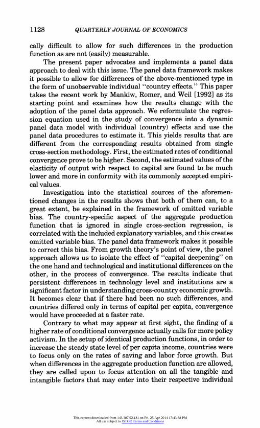
FIGURE I
Scatter Plot Matrix of in y6O, in aO, and in y85
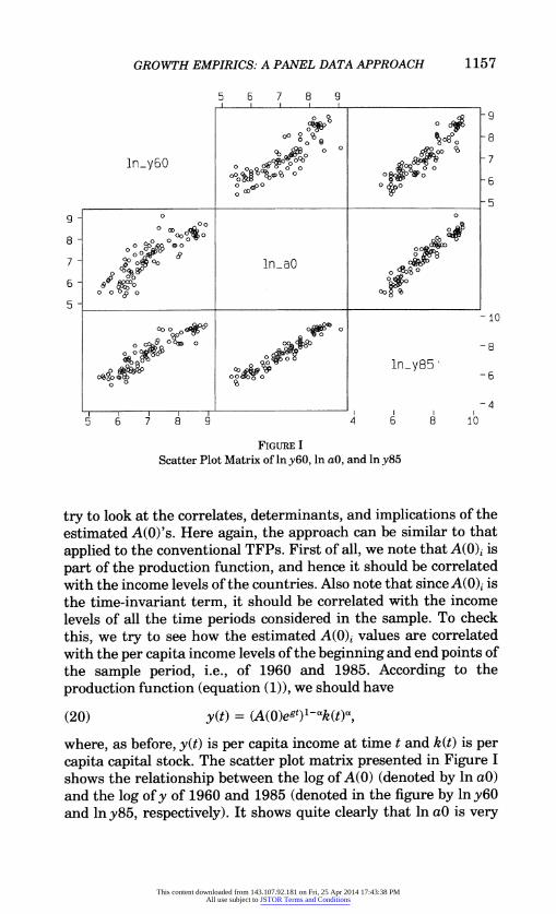
try to look at the correlates, determinants, and implications of the estimated A(O)'s. Here again, the approach can be similar to that applied to the conventional TFPs. First of all, we note that A(O)i is part of the production function, and hence it should be correlated with the income levels of the countries. Also note that since A(O)4 is the time-invariant term, it should be correlated with the income levels of all the time periods considered in the sample. To check this, we try to see how the estimated A(0)i values are correlated with the per capita income levels of the beginning and end points of the sample period, i.e., of 1960 and 1985. According to the production function (equation (1)), we should have
(20) y(t) = ((~g)1-k(~
where, as before, y(t) is per capita income at time t and k(t) is per capita capital stock. The scatter plot matrix presented in Figure I shows the relationship between the log of A(O) (denoted by ln aG) and the log of y of 1960 and 1985 (denoted in the figure by lniy6 and lny85, respectively). It shows quite clearly that ln aO is very
This content downloaded from 143.107.92.181 on Fri, 25 Apr 2014 17:43:38 PMAll use subject to JSTOR Terms and Conditions

1158 QUARTERLY JOURNAL OF ECONOMICS
closely associated with both in y6O and in y85. The simple correla- tion coefficients are 0.8656 and 0.9599 for they's of 1960 and 1985, respectively. Note that the association between ln y60 and ln y85 themselves is very strong. This can be seen from the upper right or lower left blocks of the scatter plot matrix. The simple correlation coefficient between the two is 0.9202.12
Of course, one weakness of the above evidence is that we do not have independent measures of A(0). The values of A(0) used to determine the correlations are the outcome of an estimation process in which values of y(t) themselves (along with other variables) served as the data. Therefore, there may be an induced element in the correlations cited above. However, even after discounting for such a possibility, the strength of the correlations probably remains very strong.
Next we turn to the issue of growth rates. Is the A(0) term important in explaining growth? According to the Solow-Cass- Koopmans model, steady state growth is given by the exogenous rate of technical progress. Hence, the focus here is on growth in transition. Can A(0) affect transitional growth? Note that since A(O) enters the production function in a multiplicative way, upon log differencing of y(t) of any two time periods it would vanish. As we can see from equation (20),
(21) lny(t2) - lny(t2) = (1 - 0042 - t1) + a(ln k(t2) - In k(tj)).
There is no A(0) term on the right-hand side of the above equation. This may create the impression that A(0) should not have any effect on growth. However, according to the model, the countries move toward their respective steady states, and, once that is taken into consideration, the situation changes. We have already seen in equation (10) that A(0) appears as one of the right-hand-side variables in explaining the dynamics around steady state. How- ever, in that equation, y(t1) also appears as another explanatory variable, and sincey(t1) carries anA(0) term embodied in it, the role of A(0) in the relationship gets somewhat confounded. We can make this relationship clearer in the following way. The formula
12. This strong correlation between in y60 and in y85 is noteworthy. It seems to suggest that the ranking of an economy in terms of per capita income in 1960 is almost sufficient to predict its corresponding rank in 1985. These correlations also suggest that persistent difference in the steady state levels of income because of differences in A(0) is the most salient feature of cross-country growth. The differences in A(0) outweigh the impact of relative changes across countries in other variables, like saving rate etc. Put bluntly, improvement in A(O) seems to be more important than raising the saving rate in changing the relative position of a country.
This content downloaded from 143.107.92.181 on Fri, 25 Apr 2014 17:43:38 PMAll use subject to JSTOR Terms and Conditions
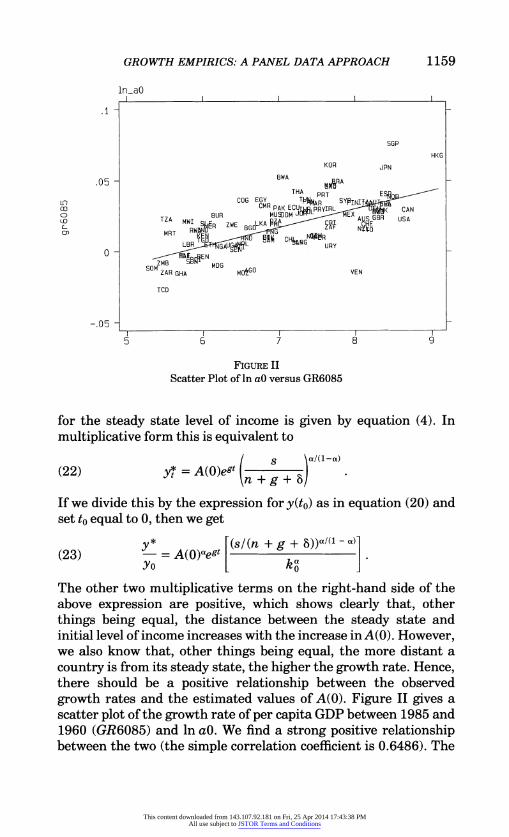
GROWTH EMPIRICS: A PANEL DATA APPROACH 1159
ln-aO
SGP
HKG KOR JPN
.05 - BWA OMRA
THA PPT ESP On
COG EGY TP*AR SYPINI 0
Go JW~~~~~~~~~~MPPK ChLPPYIRL KCAN CD SUP MUSDOM J LI CO0 TZA MWI Z E LAMIO . XAUS GSP USA CD PS E ZE L P ~ YE
CD ~~~~~MPT SWODB G NG N$p
LSP FIGURL URY
Scate Plot GflO vesuEN68
ZAP GHA mo~G E
TCD
-.05
5 6 7 8
FIGURE II Scatter Plot of In aO versus GR6085
for the steady state level of income is given by equation (4). In multiplicative form this is equivalent to
I S OA/(-a) (22) A()e + + Yt ~~ n + g + 6
If we divide this by the expression for y(to) as in equation (20) and set to equal to 0, then we get
y (s/(n + g +))a/( - a) (23) Yo = A(0)aegt k g
The other two multiplicative terms on the right-hand side of the above expression are positive, which shows clearly that, other things being equal, the distance between the steady state and initial level of income increases with the increase in A(0). However, we also know that, other things being equal, the more distant a country is from its steady state, the higher the growth rate. Hence, there should be a positive relationship between the observed growth rates and the estimated values of A(O). Figure II gives a scatter plot of the growth rate of per capita GDP between 1985 and 1960 (GR6085) and In aG. We find a strong positive relationship between the two (the simple correlation coefficient is 0.6486). The
This content downloaded from 143.107.92.181 on Fri, 25 Apr 2014 17:43:38 PMAll use subject to JSTOR Terms and Conditions
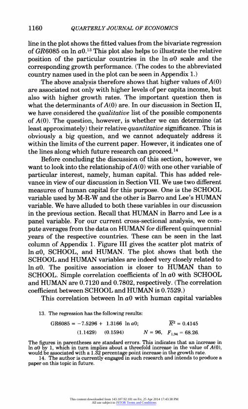
1160 QUARTERLY JOURNAL OF ECONOMICS
line in the plot shows the fitted values from the bivariate regression of GR6085 on In a0.13 This plot also helps to illustrate the relative position of the particular countries in the In a0 scale and the corresponding growth performance. (The codes to the abbreviated country names used in the plot can be seen in Appendix 1.)
The above analysis therefore shows that higher values of A(0) are associated not only with higher levels of per capita income, but also with higher growth rates. The important question then is what the determinants of A(0) are. In our discussion in Section II, we have considered the qualitative list of the possible components of A(0). The question, however, is whether we can determine (at least approximately) their relative quantitative significance. This is obviously a big question, and we cannot adequately address it within the limits of the current paper. However, it indicates one of the lines along which future research can proceed.14
Before concluding the discussion of this section, however, we want to look into the relationship of A(0) with one other variable of particular interest, namely, human capital. This has added rele- vance in view of our discussion in Section VII. We use two different measures of human capital for this purpose. One is the SCHOOL variable used by M-R-W and the other is Barro and Lee's HUMAN variable. We have alluded to both these variables in our discussion in the previous section. Recall that HUMAN in Barro and Lee is a panel variable. For our current cross-sectional analysis, we com- pute averages from the data on HUMAN for different quinquennial years of the respective countries. These can be seen in the last column of Appendix 1. Figure III gives the scatter plot matrix of ln a, SCHOOL, and HUMAN. The plot shows that both the SCHOOL and HUMAN variables are indeed very closely related to In aG. The positive association is closer to HUMAN than to SCHOOL. Simple correlation coefficients of In a0 with SCHOOL and HUMAN are 0.7120 and 0.7802, respectively. (The correlation coefficient between SCHOOL and HUMAN is 0.7529.)
This correlation between In a0 with human capital variables
13. The regression has the following results:
GR6085 = -7.5296 + 1.3166 lnaO; = 0.4145
(1.1429) (0.1594) N = 96, F194 = 68.26.
The figures in parentheses are standard errors. This indicates that an increase in In aO by 1, which in turn implies about a threefold increase in the value of A(0), would be associated with a 1.32 percentage point increase in the growth rate.
14. The author is currently engaged in such research and intends to produce a paper on this topic in future.
This content downloaded from 143.107.92.181 on Fri, 25 Apr 2014 17:43:38 PMAll use subject to JSTOR Terms and Conditions

GROWTH EMPIRICS: A PANEL DATA APPROACH 1161
5 6 7 8 9
15
o~~~~~~o~ ~ 8 o 0 o 10
school ~~~~~~ 0 0 0 0 0 0 G 0 00 0 a% 0 0 0 0 5
0 0 0 05 0 510 scho0
Scatter~ ~~~ Plo Mari of SCOL l0 a, an5UA
0 ~~~~~~~0 r
0O~~~% o~~~oR 00
0 0 ~~ 0 oo~~~,,o -10 9
0 0~~~0
obtain e ha - 5 i
0 8 ,000070000
Oc~~~Q3 ~ 0 0 0 0
6 0~~~~~~~~~~~~o
10 15 -0~0 0 ~~~~~~0 51
(single) cross-section regression, the variation in the SCHOOL variable interacts with only the cross-sectional variations of other variables. In a panel framework, on the other hand, the individual effects force the regression results to be derived more from the within variation (which is what conditional convergence is sup- posed to capture). This produces the higher rates of convergence, something that was not obtained in M-R-W.
This also helps illuminate the question that we posed toward the end of Section IV, namely, "In What Exact Way" does human capital play its role in the growth process? The close relation between the estimated values of ln A(O)i and either SCHOOL or HUMAN variable seems to suggest that the channel through which human capital affects growth may be more tortuous than that implied by its simple multiplicative inclusion in the production function with a different exponent. Instead, evidence indicates that
This content downloaded from 143.107.92.181 on Fri, 25 Apr 2014 17:43:38 PMAll use subject to JSTOR Terms and Conditions
1162 QUARTERLY JOURNAL OF ECONOMICS
this channel most likely runs through A. Of course, this does not resolve the question quoted above, but it perhaps at least indicates where to look for the answer.
IX. CONCLUSION
We argued for and implemented a panel data approach to the study of cross-country growth, in particular, of the phenomenon of convergence. This results in higher rates of conditional conver- gence and lower values of the elasticity of output with respect to capital. These results are explainable in terms of correction for omitted variable bias involved with the single cross-section regres- sion. From growth theory's point of view, they highlight the significance of the differences in the aggregate production functions.
However, the faster convergence that we observe is condi- tional. So to speak, this reveals the flip side of our finding. By being more successful (through the panel framework) in controlling for further sources of difference in the steady state levels of income, we have, at the same time, made the obtained convergence hollower. This is because convergence is more commonly understood as different countries of the world approaching the same or similar levels of income (i.e., in the "absolute" sense). There is probably little solace to be derived from finding that countries in the world are converging at a faster rate, when the points to which they are converging remain very different.
This also sheds light on the issue of policy activism. The faster rate of convergence may appear to reinforce the policy-irrelevance ethos ascribed to the Solow model. In actuality, however, the opposite is the case. Traditionally, only the saving and population growth rates were thought to be the variables for policies to be directed to. However, our study highlights the role of the A(O) term as a determinant of the steady state level of income. It thus brings to the fore the fact that, even with similar rates of saving and population growth, a country can directly improve its long-run economic position by bringing about improvements in the compo- nents of A(0). Also, improvements in A(O) can have salutary effects on s and n leading to a further (indirect) increase in the steady state level of income. Therefore, this study points to a richer scope for policies in raising the long-run income levels of countries and in quickening the pace of reaching them. One of the distinguishing aspects of development economics as a branch of economics has been its emphasis on and discussion of the elements that enter into
This content downloaded from 143.107.92.181 on Fri, 25 Apr 2014 17:43:38 PMAll use subject to JSTOR Terms and Conditions
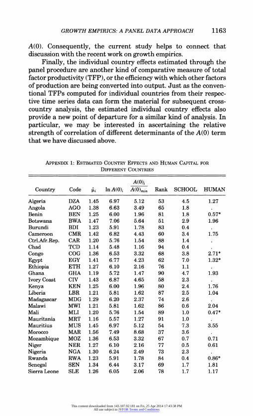
GROWTH EMPIRICS: A PANEL DATA APPROACH 1163
A(O). Consequently, the current study helps to connect that discussion with the recent work on growth empirics.
Finally, the individual country effects estimated through the panel procedure are another kind of comparative measure of total factor productivity (TFP), or the efficiency with which other factors of production are being converted into output. Just as the conven- tional TFPs computed for individual countries from their respec- tive time series data can form the material for subsequent cross- country analysis, the estimated individual country effects also provide a new point of departure for a similar kind of analysis. In particular, we may be interested in ascertaining the relative strength of correlation of different determinants of the A(O) term that we have discussed above.
APPENDIX 1: ESTIMATED COUNTRY EFFECTS AND HUMAN CAPITAL FOR DIFFERENT COUNTRIES
A(0)j Country Code i In A(0)i A(0)min Rank SCHOOL HUMAN
Algeria DZA 1.45 6.97 5.12 53 4.5 1.27 Angola AGO 1.38 6.63 3.49 65 1.8 Benin BEN 1.25 6.00 1.96 81 1.8 0.57* Botswana BWA 1.47 7.06 5.64 51 2.9 1.96 Burundi BDI 1.23 5.91 1.78 83 0.4 Cameroon CMR 1.42 6.82 4.43 60 3.4 1.75 Ctrl.Afr.Rep. CAR 1.20 5.76 1.54 88 1.4 Chad TCD 1.14 5.48 1.16 94 0.4 Congo COG 1.36 6.53 3.32 68 3.8 2.71* Egypt EGY 1.41 6.77 4.23 62 7.0 1.32* Ethiopia ETH 1.27 6.10 2.16 76 1.1 Ghana GHA 1.19 5.72 1.47 90 4.7 1.93 Ivory Coast CIV 1.43 6.87 4.65 58 2.3 Kenya KEN 1.25 6.00 1.96 80 2.4 1.76 Liberia LBR 1.21 5.81 1.62 87 2.5 1.04 Madagascar MDG 1.29 6.20 2.37 74 2.6 Malawi MWI 1.21 5.81 1.62 86 0.6 2.04 Mali MLI 1.20 5.76 1.54 89 1.0 0.47* Mauritania MRT 1.16 5.57 1.27 91 1.0 Mauritius MUS 1.45 6.97 5.12 54 7.3 3.55 Morocco MAR 1.56 7.49 8.68 37 3.6 Mozambique MOZ 1.36 6.53 3.32 67 0.7 0.71 Niger NER 1.27 6.10 2.16 77 0.5 0.61 Nigeria NGA 1.30 6.24 2.49 73 2.3 Rwanda RWA 1.23 5.91 1.78 84 0.4 0.86* Senegal SEN 1.34 6.44 3.17 69 1.7 1.81 Sierra Leone SLE 1.26 6.05 2.06 78 1.7 1.17
This content downloaded from 143.107.92.181 on Fri, 25 Apr 2014 17:43:38 PMAll use subject to JSTOR Terms and Conditions
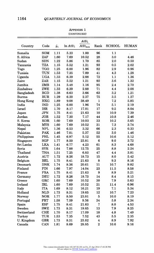
1164 QUARTERLY JOURNAL OF ECONOMICS
APPENDIX 1
(CONTINUED)
A(0)i Country Code pi In A(0)j A(0)min Rank SCHOOL HUMAN
Somalia SOM 1.11 5.33 1.00 96 1.1 S. Africa ZAF 1.60 7.69 10.52 28 3.0 4.46 Sudan SDN 1.22 5.86 1.70 85 2.0 0.50 Tanzania TZA 1.15 5.52 1.21 93 0.5 2.02 Togo TGO 1.25 6.00 1.96 82 2.9 0.96 Tunisia TUN 1.53 7.35 7.89 41 4.3 1.28 Uganda UGA 1.33 6.39 2.88 72 1.1 1.36 Zaire ZAR 1.15 5.52 1.21 92 3.6 1.32 Zambia ZMB 1.14 5.48 1.16 95 2.4 2.70 Zimbabwe ZWE 1.33 6.39 2.88 71 4.4 2.08 Bangladesh BGD 1.38 6.63 3.66 63 3.2 1.21 Burma BUR 1.29 6.20 2.37 75 3.5 1.27 Hong Kong HKG 1.89 9.08 38.49 1 7.2 5.85 India IND 1.25 6.00 1.96 74 5.1 2.19 Israel ISR 1.70 8.17 17.01 17 9.5 8.04 Japan JPN 1.75 8.41 21.63 10 10.9 7.39 Jordan JOR 1.52 7.30 7.17 44 10.8 2.46 S. Korea KOR 1.60 7.69 10.03 33 10.2 5.65 Malaysia MYS 1.60 7.69 10.52 31 7.3 3.74 Nepal NPL 1.36 6.53 3.32 66 2.3 0.33 Pakistan PAK 1.46 7.01 5.37 52 3.0 1.46 Philippines PHL 1.45 6.97 5.12 55 10.6 5.12 Singapore SGP 1.77 8.50 23.81 6 9.0 3.72 Sri Lanka LKA 1.41 6.77 4.23 61 8.3 4.68 Syria SYR 1.64 7.88 12.75 25 8.8 2.24 Thailand THA 1.51 7.25 6.83 47 4.4 3.81 Austria AUT 1.72 8.26 18.73 15 8.0 5.42 Belgium BEL 1.75 8.41 21.63 8 9.3 8.16 Denmark DNK 1.74 8.36 20.61 11 10.7 9.82 Finland FIN 1.66 7.97 14.04 23 11.5 8.58 France FRA 1.75 8.41 21.63 9 8.9 5.21 Germany DEU 1.72 8.26 18.73 14 8.4 8.15 Greece GRC 1.60 7.69 10.52 30 7.9 5.63 Ireland IRL 1.60 7.69 10.52 21 11.4 6.96 Italy ITA 1.69 8.12 16.21 19 7.1 5.34 Holland NLD 1.73 8.31 19.65 12 10.7 7.23 Norway NOR 1.77 8.50 23.81 5 10.0 8.19 Portugal PRT 1.58 7.59 9.56 34 5.8 2.34 Spain ESP 1.75 8.41 21.63 7 8.0 4.53 Sweden SWE 1.73 8.31 19.65 13 7.9 8.25 Switzerland CHE 1.70 8.17 17.09 18 4.8 7.49 Turkey TUR 1.53 7.35 7.52 43 5.5 2.35 U. Kingdom GBR 1.73 8.31 23.82 4 8.9 7.92 Canada CAN 1.81 8.69 28.85 2 10.6 9.16
This content downloaded from 143.107.92.181 on Fri, 25 Apr 2014 17:43:38 PMAll use subject to JSTOR Terms and Conditions
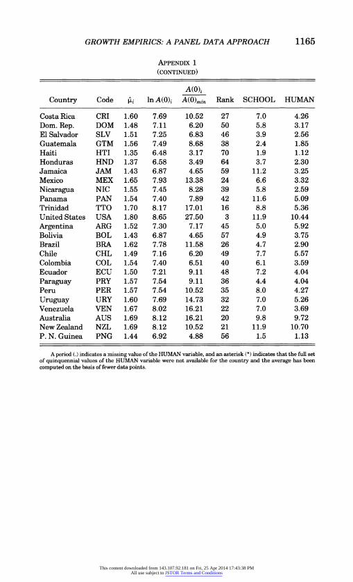
GROWTH EMPIRICS: A PANEL DATA APPROACH 1165
APPENDIX 1 (CONTINUED)
A(0)i Country Code pi In A(0)i A(0)min Rank SCHOOL HUMAN
Costa Rica CRI 1.60 7.69 10.52 27 7.0 4.26 Dom. Rep. DOM 1.48 7.11 6.20 50 5.8 3.17 El Salvador SLV 1.51 7.25 6.83 46 3.9 2.56 Guatemala GTM 1.56 7.49 8.68 38 2.4 1.85 Haiti HTL 1.35 6.48 3.17 70 1.9 1.12 Honduras HND 1.37 6.58 3.49 64 3.7 2.30 Jamaica JAM 1.43 6.87 4.65 59 11.2 3.25 Mexico MEX 1.65 7.93 13.38 24 6.6 3.32 Nicaragua NIC 1.55 7.45 8.28 39 5.8 2.59 Panama PAN 1.54 7.40 7.89 42 11.6 5.09 Trinidad TTO 1.70 8.17 17.01 16 8.8 5.36 United States USA 1.80 8.65 27.50 3 11.9 10.44 Argentina ARG 1.52 7.30 7.17 45 5.0 5.92 Bolivia BOL 1.43 6.87 4.65 57 4.9 3.75 Brazil BRA 1.62 7.78 11.58 26 4.7 2.90 Chile CHL 1.49 7.16 6.20 49 7.7 5.57 Colombia COL 1.54 7.40 6.51 40 6.1 3.59 Ecuador ECU 1.50 7.21 9.11 48 7.2 4.04 Paraguay PRY 1.57 7.54 9.11 36 4.4 4.04 Peru PER 1.57 7.54 10.52 35 8.0 4.27 Uruguay URY 1.60 7.69 14.73 32 7.0 5.26 Venezuela VEN 1.67 8.02 16.21 22 7.0 3.69 Australia AUS 1.69 8.12 16.21 20 9.8 9.72 New Zealand NZL 1.69 8.12 10.52 21 11.9 10.70 P. N. Guinea PNG 1.44 6.92 4.88 56 1.5 1.13
A period (.) indicates a missing value of the HUMAN variable, and an asterisk (*) indicates that the full set of quinquennial values of the HUMAN variable were not available for the country and the average has been computed on the basis of fewer data points.
This content downloaded from 143.107.92.181 on Fri, 25 Apr 2014 17:43:38 PMAll use subject to JSTOR Terms and Conditions
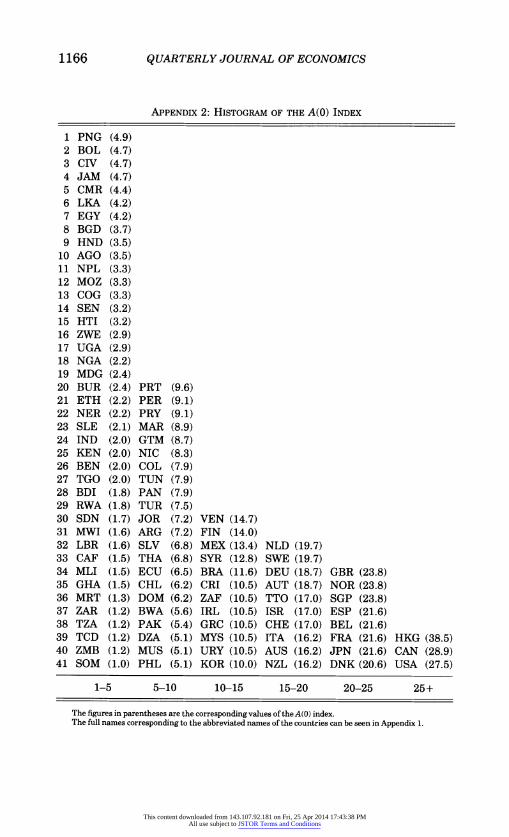
1166 QUARTERLY JOURNAL OF ECONOMICS
APPENDIX 2: HISTOGRAM OF THE A(0) INDEX
1 PNG (4.9) 2 BOL (4.7) 3 CIV (4.7) 4 JAM (4.7) 5 CMR (4.4) 6 LKA (4.2) 7 EGY (4.2) 8 BGD (3.7) 9 HND (3.5)
10 AGO (3.5) 11 NPL (3.3) 12 MOZ (3.3) 13 COG (3.3) 14 SEN (3.2) 15 HTI (3.2) 16 ZWE (2.9) 17 UGA (2.9) 18 NGA (2.2) 19 MDG (2.4) 20 BUR (2.4) PRT (9.6) 21 ETH (2.2) PER (9.1) 22 NER (2.2) PRY (9.1) 23 SLE (2.1) MAR (8.9) 24 IND (2.0) GTM (8.7) 25 KEN (2.0) NIC (8.3) 26 BEN (2.0) COL (7.9) 27 TGO (2.0) TUN (7.9) 28 BDI (1.8) PAN (7.9) 29 RWA (1.8) TUR (7.5) 30 SDN (1.7) JOR (7.2) VEN (14.7) 31 MWI (1.6) ARG (7.2) FIN (14.0) 32 LBR (1.6) SLV (6.8) MEX (13.4) NLD (19.7) 33 CAF (1.5) THA (6.8) SYR (12.8) SWE (19.7) 34 MLI (1.5) ECU (6.5) BRA (11.6) DEU (18.7) GBR (23.8) 35 GHA (1.5) CHL (6.2) CRI (10.5) AUT (18.7) NOR (23.8) 36 MRT (1.3) DOM (6.2) ZAF (10.5) TTO (17.0) SGP (23.8) 37 ZAR (1.2) BWA (5.6) IRL (10.5) ISR (17.0) ESP (21.6) 38 TZA (1.2) PAK (5.4) GRC (10.5) CHE (17.0) BEL (21.6) 39 TCD (1.2) DZA (5.1) MYS (10.5) ITA (16.2) FRA (21.6) HKG (38.5) 40 ZMB (1.2) MUS (5.1) URY (10.5) AUS (16.2) JPN (21.6) CAN (28.9) 41 SOM (1.0) PHL (5.1) KOR (10.0) NZL (16.2) DNK (20.6) USA (27.5)
1-5 5-10 10-15 15-20 20-25 25+
The figures in parentheses are the corresponding values of the A() index. The full names corresponding to the abbreviated names of the countries can be seen in Appendix 1.
This content downloaded from 143.107.92.181 on Fri, 25 Apr 2014 17:43:38 PMAll use subject to JSTOR Terms and Conditions
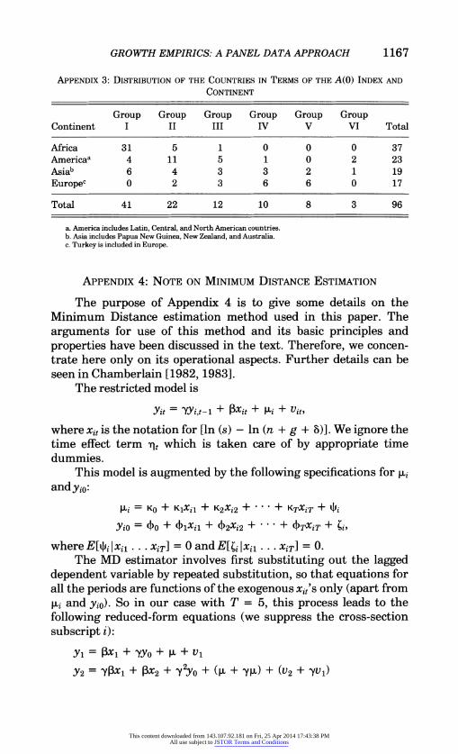
GROWTH EMPIRICS: A PANEL DATA APPROACH 1167
APPENDIX 3: DISTRIBUTION OF THE COUNTRIES IN TERMS OF THE A(0) INDEX AND
CONTINENT
Group Group Group Group Group Group Continent I II III IV V VI Total
Africa 31 5 1 0 0 0 37 Americaa 4 11 5 1 0 2 23 Asiab 6 4 3 3 2 1 19 Europec 0 2 3 6 6 0 17
Total 41 22 12 10 8 3 96
a. America includes Latin, Central, and North American countries. b. Asia includes Papua New Guinea, New Zealand, and Australia. c. Turkey is included in Europe.
APPENDIX 4: NOTE ON MINIMUM DISTANCE ESTIMATION
The purpose of Appendix 4 is to give some details on the Minimum Distance estimation method used in this paper. The arguments for use of this method and its basic principles and properties have been discussed in the text. Therefore, we concen- trate here only on its operational aspects. Further details can be seen in Chamberlain [1982, 1983].
The restricted model is
=it = Yit- + Pxit + ki + Vito
where xi, is the notation for [in (s) - in (n + g + r)]. We ignore the time effect term 9t which is taken care of by appropriate time dummies.
This model is augmented by the following specifications for pi andyio:
i= Ko + K0Xij + K2Xi2 + + KTXiT + PIi
YiO = ko + kXil + 4)2Xi2 + + 4)TXiT + hi,
where E[4ij lxi, . . . XiT] = 0 and E[4 Ixi1 . . . XiT] = 0. The MD estimator involves first substituting out the lagged
dependent variable by repeated substitution, so that equations for all the periods are functions of the exogenous xit's only (apart from pi and Yio). So in our case with T = 5, this process leads to the following reduced-form equations (we suppress the cross-section subscript i):
Y1 = AX1 + YY0 + RL + Vi
Y2 = 'SYPX1 + r3X2 + Y2Yo + (R + mYa) + (v2 + _yV1)
This content downloaded from 143.107.92.181 on Fri, 25 Apr 2014 17:43:38 PMAll use subject to JSTOR Terms and Conditions

1168 QUARTERLY JOURNAL OF ECONOMICS
y3 =2pX + -YPX2 + 3X3 + Y3Y0 + (p + _yp + _y2p)
+ (V3 + YV2 + y2V,)
y4 = y3X1 + _y2 X2 + _YPX3 + PX4 + Y4Y0
+ (pL + yp. + -y2p + y3R) + (v4 + yv3 + y2V2 + y3v,)
Y5 = y43X + _y3 X2 + y2r3X3 + _Y x4 + 3X5 + Y 5Yo + (R + ,yi + ,y2p + ,y3p + y4R)
+ (v5 + yv4 + y2v3 + y3v2 + y4V1).
In matrix form this may be expressed as
Y1 0 0 0 ? x1 Y Y2 Syj3 B 3 0 0 0 x2 Y3 Y 213 _y3 13 0 O x3 + Y3 Y0
Y4 ly3 y2 _y I 0 x4 y4
Y5 y41 y3r _y2r _y1 p i X5 y5
1 U1
1+ y U2
+ l+ y+ y2 + Ut3
1+y+y2+y3 u4
1+y+y2+y3+y4 U5
where ut stands for the respective composite error term consisting of vi's. Now, if we substitute for yo and ,u per their specifications adopted above, then we get the Il-matrix of the reduced-form coefficients of the following form:
IP 0 0 0 0 y (3 0 0 0 ~2
-y3 ~2p _ p 0 + y 'y$3 _y3 ~2 p _ p 0 3
1+ y
1 + y + y2 + y3 l + y + y2 )K.y
+ y + y2 + y3 + y4
If xe's are strictly exogenous, then they are uncorrelated with the
This content downloaded from 143.107.92.181 on Fri, 25 Apr 2014 17:43:38 PMAll use subject to JSTOR Terms and Conditions
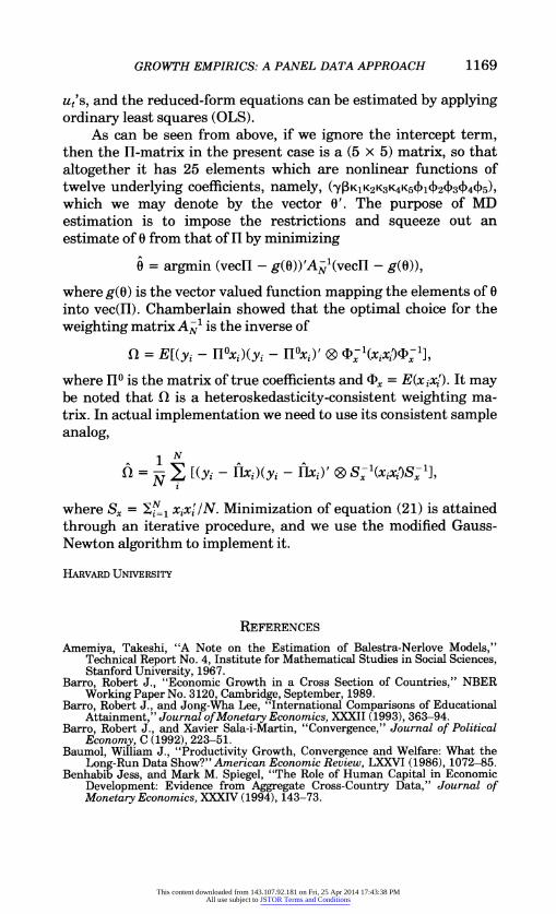
GROWTH EMPIRICS: A PANEL DATA APPROACH 1169
ut's, and the reduced-form equations can be estimated by applying ordinary least squares (OLS).
As can be seen from above, if we ignore the intercept term, then the Hl-matrix in the present case is a (5 x 5) matrix, so that altogether it has 25 elements which are nonlinear functions of twelve underlying coefficients, namely, (ypKlK2K3K4K5+l+2+3+4+5), which we may denote by the vector 0'. The purpose of MD estimation is to impose the restrictions and squeeze out an estimate of 0 from that of H by minimizing
0 = argmin (vecH - g(0))'Aj1(vecHI - g(O)),
where g(O) is the vector valued function mapping the elements of 0 into vec(H). Chamberlain showed that the optimal choice for the weighting matrix AJ-1 is the inverse of
fl = E[(y, - HIxi )(yi - H0xj)' 0 -l(x'x/ l'],
where HO is the matrix of true coefficients and Fx = E(x ixj). It may be noted that ft is a heteroskedasticity-consistent weighting ma- trix. In actual implementation we need to use its consistent sample analog,
Ni= z[(Yi - Ji'xj)(Yi - ix)' 0 S;-(xixltS;1],
where Sx = V xixI'/N. Minimization of equation (21) is attained through an iterative procedure, and we use the modified Gauss- Newton algorithm to implement it.
HARVARD UNIVERSITY
REFERENCES
Amemiya, Takeshi, "A Note on the Estimation of Balestra-Nerlove Models," Technical Report No. 4, Institute for Mathematical Studies in Social Sciences, Stanford University, 1967.
Barro, Robert J., "Economic Growth in a Cross Section of Countries," NBER Working Paper No. 3120, Cambridge, September, 1989.
Barro, Robert J., and Jong-Wha Lee, "International Comparisons of Educational Attainment," Journal of Monetary Economics, XXXII (1993), 363-94.
Barro, Robert J., and Xavier Sala-i-Martin, "Convergence," Journal of Political Economy, C (1992),223-51.
Baumol, William J., "Productivity Growth, Convergence and Welfare: What the Long-Run Data Show?" American Economic Review, LXXVI (1986), 1072-85.
Benhabib Jess, and Mark M. Spiegel, "The Role of Human Capital in Economic Development: Evidence from Aggregate Cross-Country Data," Journal of Monetary Economics, XXXIV (1994), 143-73.
This content downloaded from 143.107.92.181 on Fri, 25 Apr 2014 17:43:38 PMAll use subject to JSTOR Terms and Conditions
1170 QUARTERLY JOURNAL OF ECONOMICS
Cass, David, "Optimum Growth in an Aggregative Model of Capital Accumulation," Review of Economic Studies, XXXII (1965), 233-40.
Chamberlain, Gary, "Multivariate Regression Models for Panel Data," Journal of Econometrics, XVIII (1982), 5-46.
"Panel Data," in Handbook of Econometrics, Zvi Griliches and Michael Intriligator, eds. (Amsterdam: North-Holland, 1983), pp. 1247-1318.
Chua, Hak B., "Regional Spillovers and Economic Growth," Department of Economics, Harvard University, 1992.
De Gregorio, Jose, "Economic Growth in Latin America," Journal of Development Economics, XXXIX (1992), 59-84.
De Long, J. Bradford, "Productivity Growth, Convergence, and Welfare, American Economic Review, LXXIX (1989), 1010-30.
Durlauf, S., and P. A. Johnson, "Local and Global Convergence across National Economies," Department of Economics, Stanford University, 1991.
Islam, Nazrul, "Estimation of Dynamic Models from Panel Data: A Review," Department of Economics, Harvard University, 1991. ,"Small Sample Performance of Dynamic Panel Data Estimators: A Monte Carlo Study," Department of Economics, Harvard University, 1992.
King, Robert G., and Sergio T. Rebelo, "Transitional Dynamics and Economic Growth in the Neoclassical Model," NBER Working Paper No. 3185, Cam- bridge, 1989.
Koopmans, T. C., "On the Concept of Optimal Economic Growth," in The Economic Approach to Development Planning, Pontifical Academy of Sciences (Amster- dam: North-Holland, 1965).
Maddala, G. S., "The Use of Variance Components Model in Pooling Cross-Section and Time Series Data," Econometrica, XXXIX (1971), 341-58.
Maddison, A., Phases of Capitalist Development (Oxford: Oxford University Press, 1982).
Mankiw, N. Gregory, David Romer, and David Weil, "A Contribution to the Empirics of Economic Growth," Quarterly Journal of Economics, CVII (1992), 407-37.
Mundlak, Yari, "On the Pooling of Time Series and Cross-Section Data," Economet- rica, XXXVI (1978), 69-85.
Rebelo, Sergio, "Long-Run Policy Analysis and Long-Run Growth," Journal of Political Economy, XCIX (1991), 500-21.
Romer, Paul, "Capital Accumulation in the Theory of Long-Run Growth," in Modern Business Cycle Theory, Robert J. Barro, ed. (Cambridge, MA: Harvard University Press, 1989a). ,"Human Capital and Growth: Theory and Evidence," NBER Working Paper No. 3173, Cambridge, 1989b.
Solow, Robert M., "A Contribution to the Theory of Economic Growth," Quarterly Journal of Economics, LXX (1956), 65-94.
Summers, Robert, and Alan Heston, "A New Set of International Comparisons of Real Product and Price Levels Estimates for 130 Countries, 1950-85," Review of Income and Wealth, XXXIV (1988), 1-26.
Young, Alwyn, "A Tale of Two Cities: Factor Accumulation and Technical Change in Hong Kong and Singapore," in NBER Macroeconomics Annual 1992, Olivier J. Blanchard and Stanley Fischer, eds. (Cambridge, MIT Press, 1992), pp. 13- 54.
"The Tyranny of Numbers: Confronting the Statistical Realities of the East Asian Growth Experience," Quarterly Journal of Economics, CX (1995), 641-80.
This content downloaded from 143.107.92.181 on Fri, 25 Apr 2014 17:43:38 PMAll use subject to JSTOR Terms and Conditions