Embed Size (px)
Citation preview

Staples Equity Valuation and Analysis
David Lecky
Chad Loudermilk
Bennett Matkins
Kara Reynolds
Amanda Rhodes

1
Table of Contents Executive Summary……………………………………………………….. 2 Overview of Staples and the Industry………………………………... 7 Five Forces Model……………………………………………………………………….. 9 Rivalry among Existing Firms……………………………………………………….. 9 Threat of New Entrants……………………………………………………………….. 15 Threat of Substitute Products………………………………………………………. 17 Bargaining Power of Buyers………………………………………………………... 17 Bargaining Power of Suppliers…………………………………………………..... 18 Classifying the Industry………………………………………………………………. 18 Key Success Factors……………………………………………………………………. 19 Competitive Advantage Analysis………………………………………………….. 19 Accounting Analysis………………………………………………………. 25 Key Accounting Policies………………………………………………………………. 25 Accounting Flexibility………………………………………………………………….. 26 Evaluation of Actual Accounting Strategy……………………………………… 29 Quality of Disclosure…………………………………………………………………… 30 Screening Ratio Analysis….…………………………………………………………. 33 Revenue Diagnostics………………………………………………………………….. 34 Expense Diagnostics…………………………………………………………………… 37 Potential “Red Flags”………………………………………………………………….. 39 Undo Accounting Distortions……………………………………………………….. 41 Ratio Analysis………………………………………………………………. 44 Liquidity Ratio……………………………………………………………………………. 44 Profitability Ratio……………………………………………………………………….. 56 Capital Structure Ratio……………………………………………………………….. 66 SGR & IGR………………………………………………………………………………… 71 Financial Statement Forecasting……………………………………… 72 Income Statement……………………………………………………………………… 72 Balance Sheet……………………………………………………………………………. 77 Statement of Cash Flows……………………………………………………………. 80 Analysis of Evaluations………………………………………………….. 83 Cost of Capital………………………………………………………………………….. 83 Method of Comparables…………………………………………………………….. 86 Intrinsic Valuation Models………………………………………………………….. 89 Altman Z-Score…………………………………………………………………………. 96 Appendices: Appendix 1: Screening Ratios…………………………………………………….. 98 Appendix 2: Core Financial Ratios………………………………………………. 99 Appendix 3: Regression Analysis……………………………………………….. 100 Appendix 4: Valuation Models……………………………………………………. 105 Works Cited………..................................................................... 110

2
Executive Summary
Investment Recommendation: Slightly Overvalued: Hold 04/01/07
SPLS - Nasdaq $25.84 EPS Forecast52 week range $21.08 - $28.00 FYE 4/1 2006 (A) 2007 (E) 2008 (E) 2009 (E)Revenue (2006) $18,160,789 EPS $1.32 $1.55 $1.77 $2.01Market Capitalization $18.19 BillionShares Outstanding 717,000,000 Ratio Comparison SPLS ODP OMXDividend Yield .29 (1.1%) Trailing P/E $41.29 $55.99 $37.223-month Avg Daily Trading Vol. 6,120,780 Forward P/E $19.50 $26.44 $17.58Percent Institutional Ownership 84.60% M/B $19.78 $26.72 $72.96Book Value Per Share (mrq) $6.99ROE 22% Valuation EstimatesROA 12.68% Actual Price (as of 4/1/07) $25.84Est. 5 year EPS Growth Rate 13.95% Ratio Based ValuationsCost of Capital Est. R2 Beta Ke P/E Trailing $19.56Ke Estimated 10.24% P/E Forward $15.055-year 0.230 1.146 10.04% Enterprise Value $29.121-year 0.231 1.150 10.19% M/B $3.6810-year 0.230 1.146 9.97%3-month 0.232 1.152 10.24% Intrinsic ValuationsPublished 1.52 Discounted Dividends $3.38Kd 5.547% Free Cash Flows $20.13WACC 9.2292% Residual Income $17.07Altman Z-Score 6.88 LR ROE $12.61
Abnormal Earnings Growth $15.26
Staples stock is traded on the NASDAQ market and the ticker symbol is:
SPLS. The Company had its Initial Public Offering (I.P.O.) on April 27, 1989.
3,250,000 shares sold at $19.00 per share ($0.74 after adjusting for stock splits).
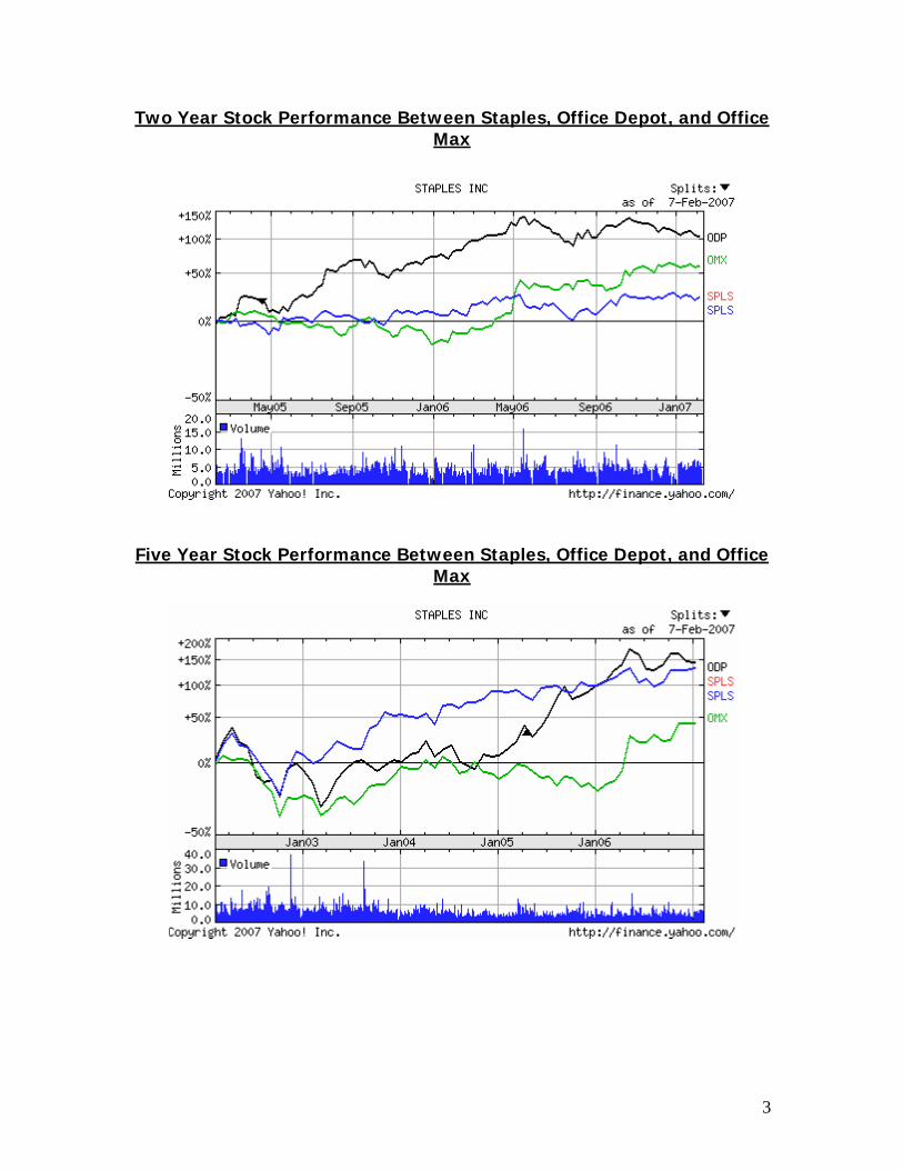
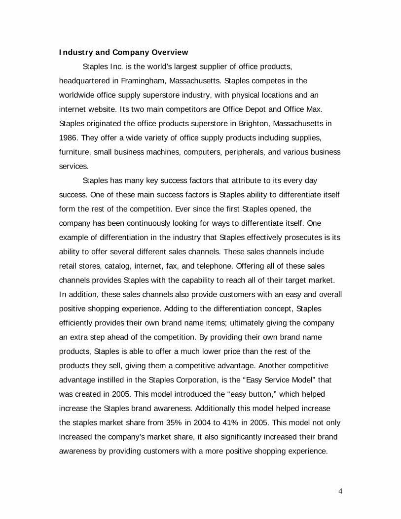
Since 2002, Staples’ stock prices have almost doubled. Their stock prices have
also been fairly consistent with that of its competitors for the past two years.
3
Two Year Stock Performance Between Staples, Office Depot, and Office Max
Five Year Stock Performance Between Staples, Office Depot, and Office Max
4
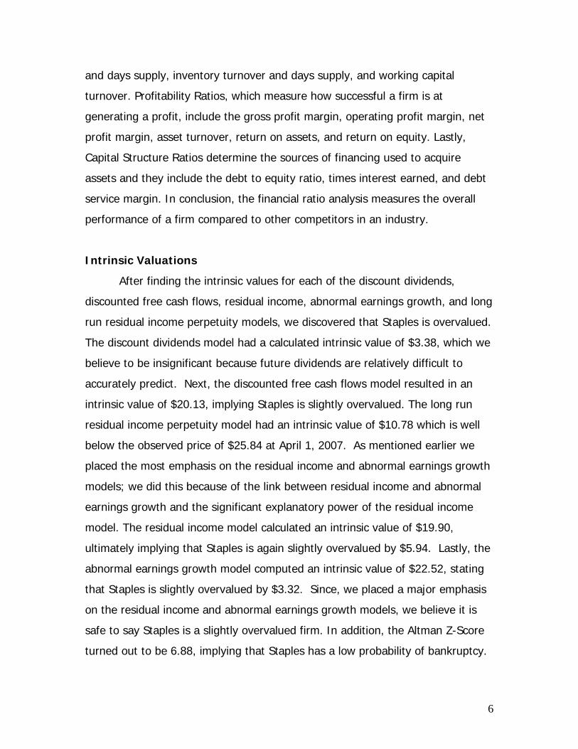
Industry and Company Overview
Staples Inc. is the world’s largest supplier of office products,
headquartered in Framingham, Massachusetts. Staples competes in the
worldwide office supply superstore industry, with physical locations and an
internet website. Its two main competitors are Office Depot and Office Max.
Staples originated the office products superstore in Brighton, Massachusetts in
1986. They offer a wide variety of office supply products including supplies,
furniture, small business machines, computers, peripherals, and various business
services.
Staples has many key success factors that attribute to its every day
success. One of these main success factors is Staples ability to differentiate itself
form the rest of the competition. Ever since the first Staples opened, the
company has been continuously looking for ways to differentiate itself. One
example of differentiation in the industry that Staples effectively prosecutes is its
ability to offer several different sales channels. These sales channels include
retail stores, catalog, internet, fax, and telephone. Offering all of these sales
channels provides Staples with the capability to reach all of their target market.
In addition, these sales channels also provide customers with an easy and overall
positive shopping experience. Adding to the differentiation concept, Staples
efficiently provides their own brand name items; ultimately giving the company
an extra step ahead of the competition. By providing their own brand name
products, Staples is able to offer a much lower price than the rest of the
products they sell, giving them a competitive advantage. Another competitive
advantage instilled in the Staples Corporation, is the “Easy Service Model” that
was created in 2005. This model introduced the “easy button,” which helped
increase the Staples brand awareness. Additionally this model helped increase
the staples market share from 35% in 2004 to 41% in 2005. This model not only
increased the company’s market share, it also significantly increased their brand
awareness by providing customers with a more positive shopping experience.

5
Accounting Analysis
Staples’ annual 10-K contains information regarding their key accounting
policies and accounting flexibility which can be used to evaluate their accounting
strategies and identify potential red flags. During the process we were able to
conclude that Staples quality of disclosure was superior to its competitors. During
the accounting analysis we were able to relate Staples’ key success factors to
their key accounting policies and identify potential red flags. For example,
Staples finances the majority of their properties with operating leases rather than
capital leases which causes the assets and liabilities to be understated. Also,
since the implementation of SFAS No. 142, Staples has acquired six different
businesses worldwide and has failed to write off any goodwill causing the assets
on the balance sheet to be overstated and the expenses on the income
statement to be understated by a significant amount. After we discovered these
accounting distortions we were able to adjust their accounting methods to
represent true values. We were able to adjust the lease problem by finding the
present value of Staples’ future payments on its operating leases, and increase
the assets and liabilities on the balance sheet by that amount. Also, we
amortized the current value of goodwill over the next ten years down to zero to
make up for Staples failure of not writing off goodwill. After undoing these
accounting distortions, Staples’ true value will be revealed.
Financial Ratio Analysis
The financial statements for a firm provide significant information that
must be evaluated to analyze their overall performance compared to other firms
in the industry. This analysis provides you with a way to relate different line
items of the financial statements and then assess those relationships. There are
three main groups of ratios: liquidity, profitability, and capital structure. Liquidity
ratios, which determine a firm’s ability to meet current obligations with liquid
assets, include the current ratio, quick asset ratio, accounts receivable turnover
6
and days supply, inventory turnover and days supply, and working capital
turnover. Profitability Ratios, which measure how successful a firm is at
generating a profit, include the gross profit margin, operating profit margin, net
profit margin, asset turnover, return on assets, and return on equity. Lastly,
Capital Structure Ratios determine the sources of financing used to acquire
assets and they include the debt to equity ratio, times interest earned, and debt
service margin. In conclusion, the financial ratio analysis measures the overall
performance of a firm compared to other competitors in an industry.
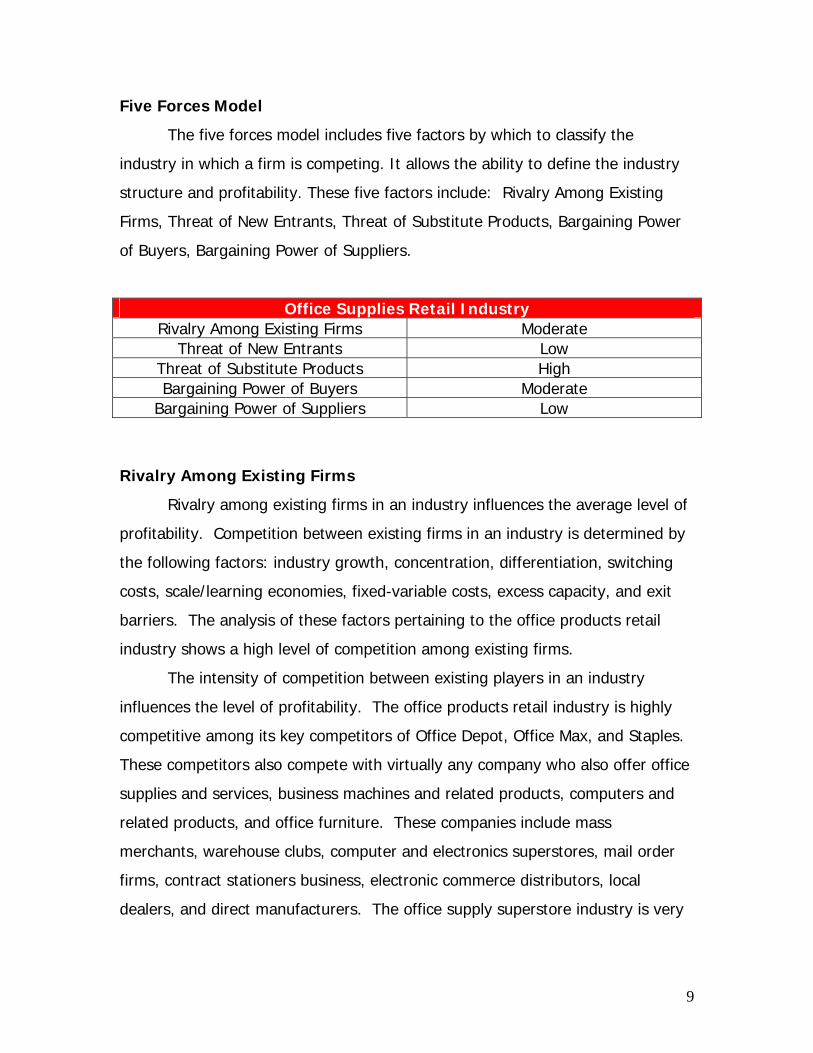
Intrinsic Valuations
After finding the intrinsic values for each of the discount dividends,
discounted free cash flows, residual income, abnormal earnings growth, and long
run residual income perpetuity models, we discovered that Staples is overvalued.
The discount dividends model had a calculated intrinsic value of $3.38, which we
believe to be insignificant because future dividends are relatively difficult to
accurately predict. Next, the discounted free cash flows model resulted in an
intrinsic value of $20.13, implying Staples is slightly overvalued. The long run
residual income perpetuity model had an intrinsic value of $10.78 which is well
below the observed price of $25.84 at April 1, 2007. As mentioned earlier we
placed the most emphasis on the residual income and abnormal earnings growth
models; we did this because of the link between residual income and abnormal
earnings growth and the significant explanatory power of the residual income
model. The residual income model calculated an intrinsic value of $19.90,
ultimately implying that Staples is again slightly overvalued by $5.94. Lastly, the
abnormal earnings growth model computed an intrinsic value of $22.52, stating
that Staples is slightly overvalued by $3.32. Since, we placed a major emphasis
on the residual income and abnormal earnings growth models, we believe it is
safe to say Staples is a slightly overvalued firm. In addition, the Altman Z-Score
turned out to be 6.88, implying that Staples has a low probability of bankruptcy.

7
The WACC was calculated to be 9.29%, with a cost of equity of 10.237% and a
cost of debt of 5.547%.
Business and Industry Analysis
Company Overview
Staples, Inc. introduced the first office products superstore in Brighton,
Massachusetts in 1986. Launched to serve the needs of small businesses,
Staples, Inc. is a specialty retailer offering a wide array of office supply products
including supplies, furniture, small business machines, computers, and
peripherals. They also offer business services such as color and self-service
copying, printing services, faxing, and pack and ship services. Staples has 1,522
superstores found in 47 states, the District of Columbia, and 11 Canadian
provinces at the fiscal year end of 2005. In addition, 258 stores are found in 19
countries in Europe, South America, and Asia. Staples is continuing to grow with
an average of 119.8 store openings per year over the past 5 years. The company
is headquartered in Framingham, Massachusetts. It also does business via the
Internet, through its own website.
Staples concentrates on superior customer services to differentiate itself
from competitors offering low prices and innovative services. In 2003, Staples
launched its new brand promise: “We make buying office products easy.”
Activating a new customer service model to its employees, offering expanded
product lines, speedy check-outs, in-stock guarantees, and redesigning their
website to make it more customer-friendly are some of the new features Staples
offers to cater to its customers. It currently leads the industry in market
capitalization at 18.6 billion dollars.

8
Staples Sales & Assets
$0
$5,000,000
$10,000,000
$15,000,000
$20,000,000
Year
$ in
Tho
usan
ds
SPLS SalesSPLS Assets
SPLS Sales $10,744,373 $11,596,075 $12,967,022 $14,448,378 $16,078,852
SPLS Assets $4,093,035 $5,721,388 $6,503,046 $7,071,448 $7,676,589
2002 2003 2004 2005 2006
The office products industry as a whole has been continuously growing
over the past four years. Office Max’s sales have declined in response to Office
Depot and Staples’ sales rapidly increasing. The industry also shows an increase
in individual company assets.
Staples Competitors Sales and Assets (Office Depot & Office Max)
$0
$2,000,000
$4,000,000
$6,000,000
$8,000,000
$10,000,000
$12,000,000
$14,000,000
$16,000,000
Year
$ in
Tho
usan
ds
ODP SalesODP AssetsOMX SalesOMX Assets
ODP Sales $11,356,633 $12,358,566 $13,564,699 $14,278,944
ODP Assets $4,765,812 $6,145,242 $6,794,338 $6,098,525
OMX Sales $7,412,330 $8,245,146 $13,270,196 $9,157,660
OMX Assets $1,295,750 $7,376,159 $7,542,999 $6,272,142
2002 2003 2004 2005
9
Five Forces Model
The five forces model includes five factors by which to classify the
industry in which a firm is competing. It allows the ability to define the industry
structure and profitability. These five factors include: Rivalry Among Existing
Firms, Threat of New Entrants, Threat of Substitute Products, Bargaining Power
of Buyers, Bargaining Power of Suppliers.
Office Supplies Retail Industry Rivalry Among Existing Firms Moderate
Threat of New Entrants Low Threat of Substitute Products High Bargaining Power of Buyers Moderate
Bargaining Power of Suppliers Low
Rivalry Among Existing Firms
Rivalry among existing firms in an industry influences the average level of
profitability. Competition between existing firms in an industry is determined by
the following factors: industry growth, concentration, differentiation, switching
costs, scale/learning economies, fixed-variable costs, excess capacity, and exit
barriers. The analysis of these factors pertaining to the office products retail
industry shows a high level of competition among existing firms.
The intensity of competition between existing players in an industry
influences the level of profitability. The office products retail industry is highly
competitive among its key competitors of Office Depot, Office Max, and Staples.
These competitors also compete with virtually any company who also offer office
supplies and services, business machines and related products, computers and
related products, and office furniture. These companies include mass
merchants, warehouse clubs, computer and electronics superstores, mail order
firms, contract stationers business, electronic commerce distributors, local
dealers, and direct manufacturers. The office supply superstore industry is very
10
competitive because the key competitors also have to compete against any
company that sells office products.
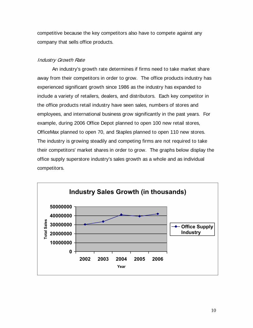
Industry Growth Rate
An industry’s growth rate determines if firms need to take market share
away from their competitors in order to grow. The office products industry has
experienced significant growth since 1986 as the industry has expanded to
include a variety of retailers, dealers, and distributors. Each key competitor in
the office products retail industry have seen sales, numbers of stores and
employees, and international business grow significantly in the past years. For
example, during 2006 Office Depot planned to open 100 new retail stores,
OfficeMax planned to open 70, and Staples planned to open 110 new stores.
The industry is growing steadily and competing firms are not required to take
their competitors’ market shares in order to grow. The graphs below display the
office supply superstore industry’s sales growth as a whole and as individual
competitors.
Industry Sales Growth (in thousands)
0
10000000
20000000
30000000
40000000
50000000
2002 2003 2004 2005 2006Year
Tota
l Sal
es
Office SupplyIndustry

11
SPLS, ODP, OMX Sales (in thousands)
0
5000000
10000000
15000000
20000000
2002 2003 2004 2005 2006Year
Sale
s StaplesOffice DepotOffice Max
Concentration and Balance of Competitors
The degree of concentration and the balance of the competitors in an
industry determine the amount of competition based upon price within the
industry. The office products retail industry’s main competitors are Office Depot,
Office Max, and Staples, but office products are also sold by various firms such
as Wal-Mart, Costco, Best Buy, and Dell. In order to compete with these firms,
office supply superstores have to keep their prices competitive, rely on superior
customer service, broader selection of office products, and convenient store
locations. Since Office Depot, OfficeMax, and Staples are the only main
competitors in the office products retail industry they often cooperate among
themselves to avoid destructive price competition. In conclusion, the office
products retail industry is highly centralized among Office Depot, OfficeMax, and
Staples. The graphs below display the market shares of these competitors in the
office supply superstore industry for the past five years.

12
Market Shares: 2002
39%
37%
24%StaplesOffice DepotOffice Max
For 2002, Staples is the leader owning 39 percent of the office supply
superstore industry. Office Depot is running a close second with 37 percent and
coming in last is OfficeMax with a much lower 24 percent.
Market Shares: 2003
38%
37%
25%StaplesOffice DepotOffice Max
In 2003, Staples remained the leader by a narrow margin of one percent
(38% of industry market share). Following close behind was Office Depot with 37
percent and once again OfficeMax was lagging behind with 25 percent.
Market Shares: 2004
35%
33%
32% StaplesOffice DepotOffice Max

13
In 2004, OfficeMax took a considerable amount of the market share from
its competitors from previous years but remained in last with 32 percent. Again
Staples was the leader in the industry with a lower 35 percent and Office Depot
followed closely with 33 percent.
Market Shares: 2005
41%
36%
23%StaplesOffice DepotOffice Max
For 2005, Staples raised the bar and increased their market share by 6
percent to 41 percent. Office Depot stayed in second with a market share of 36
percent and OfficeMax fell drastically behind to 23 percent.
Market Shares: 2006
43%
36%
21%StaplesOffice DepotOffice Max
In 2006, Staples further increased their market share by 2 percent to a
total of 43 percent. Office Depot remained the same at 36 percent, while
OfficeMax fell further behind to 21 percent.
The above graphs show Staples has remained the office supply
superstore industry’s leader for the past five years. We believe that much of this
success is derived from Staples’ ability to differentiate itself from competitors
while maintaining a low price strategy.

14
Degree of Differentiation and Switching Costs
Firms in any industry must differentiate their products and services in
order to avoid excessive competition. Firms in the office products retail industry
mainly carry identical products or close substitutes to their competitors. In
addition, Office Depot, OfficeMax, and Staples offer similar websites and in-store
copy and print services. Since the products the firms sell and the services they
offer carry a low degree of differentiation, switching costs for customer are very
low. Since, the office products retail industry offers minimal product
differentiation and low switching costs, customers are allowed to switch retailers
purely on the basis of price.
Scale/Learning Economies and the Ratio of Fixed to Variable Costs
If there are any types of scale or learning economies in an industry, firm
sizes become an important factor. When economies of scale exist in an industry,
new firms must be willing and able to invest large amounts of capital in order to
grab market share and compete with industry leaders. In the office products
retail industry there are only three main competitors and large economies of
scale exist making it difficult for new entrants in the industry to compete. Office
Depot, OfficeMax, and Staples therefore compete aggressively for market share.
A firm in any industry must minimize its variable costs in order to maintain
profits. Firms in the office products retail industry are able to obtain low variable
costs by purchasing supplies in bulk from vendors. Also, Staples is able to
further reduce their variable costs by selling their own branded products which
cost 10-15% less than national brands. Firms in the office supply superstore
industry are able to reduce their variable costs allowing them to maintain profits.
Excess Capacity and Exit Barriers
If capacity in an industry is larger than customer demand, there is a
strong incentive for firms to cut prices to fill capacity (Palepu 2-3). High levels of
inventories associated with the office products retail industry create an excess
15
capacity because it creates more supply than demand. The excess capacity can
require firms to cut prices to fill capacity. Exit barriers make it difficult and costly
for firms to exit the industry. The office products retail industry typically does
not have specialized assets or legal barriers. Therefore the exit barriers to the
industry are not costly.
Threat of New Entrants
Economies of Scale
Economies of scale exist within an industry when companies expand the
scope of their operations, resulting in a subsequent decrease in costs for
companies competing within that industry. When economies of scale exist, new
entrants must be willing to invest large amounts of capital in order to compete
with the industry’s leading companies. It is important for a company to
recognize where economies of scale exist because they help the company
understand where its resources should be allocated in order to improve market
share and increase profits. Leading companies within the office product retail
industry, such as Staples and Office Depot, specialize in selling a wide variety of
products in-store. In 2005, Staples’ merchandise inventories were 40% of the
company’s total current assets. A company entering the office products segment
of the specialty retail industry must possess bargaining power with suppliers and
enough capital to acquire, and maintain, a large in-store merchandise inventory,
or the company will not survive in the industry. Another barrier to new entrants
is their limited access to markets. Larger companies have greater access to
markets and can operate with larger geographic reach. Office Depot, for
example, operates 1,016 stores in 49 different states and plans to continue to
open new locations. Staples and its competitors benefit from economies of scale
in advertising as well. In 2005, Staples unveiled the Easy marketing message
which enhanced Staple’s brand promise to make buying office products easy.
Because of increased buying power, market accessibility, and efficient

16
advertising, large economies of scale exist within the office products segment of
the retail industry.
First Mover Advantage
In an industry where price competition and switching costs are minimal, a
company must create a first mover advantage in other aspects of the business.
For example, according to finance.yahoo.com, Office Max recently announced
that it plans on installing the newest, state-of-the art Xerox systems that will
allow customers to produce their work faster and with greater quality. In this
industry, companies create a first mover advantage by introducing innovative
customer service techniques, providing new services to customers first,
introducing new product lines, and expanding into untapped markets globally,
which can be quite costly; therefore, first mover advantage is of moderate risk.
Access to Channels of Distribution and Relationships
Companies in the office supplies retail industry differentiate themselves by
offering superior product variety. To achieve this, it is critical for companies in
this industry to implement efficient inventory methods in order to maintain on-
shelf products. Companies, such as Staples and Office Depot, receive efficient
inventory volumes through retail distribution centers that purchase products
directly from manufacturers. Many of the products sold in these stores come
from competing manufacturers which adversely affects manufacturer relations.
The result of this adverse affect could be that vendors reduce product offerings
in leading office supplies retail companies. Also, many companies in this industry
sell products sourced from a wide variety of third-party vendors, including
international manufacturers. This is a risk factor because leading companies in
this industry cannot control the availability of the raw materials used to make
their products or the stability of foreign supply chains; therefore, companies in
the office supplies retail industry face a high risk of new entrants because of
competition between manufacturers and uncontrollable third-party vendors.

17
Legal Barriers
In this specialized segment of the retail industry prospective entrants do
not face many legal barriers to entry. Licensing regulations, patents, and
copyrights are non-existent within this industry. The only legal barrier to entry is
if a prospective entrant might want to begin Internet operations. There are laws
and regulations that must be followed when conducting business transactions on
the Internet. Because of the absence of extensive legal barriers to entry, this
industry faces a high risk of entrants into the market.
Threat of Substitute Products
The threat of substitutes depends on the relative price and performance
of competing products or services and the customers’ willingness to substitute
(Palepu 2-4). The office products retail industry competes mainly on the basis of
pricing, product selection, convenient locations, and customer service.
Competitors in the industry offer identical products and services and close
substitutes. For example, Office Depot, OfficeMax, and Staples all sell similar
office supplies, technology products, and furniture to consumers. Therefore, the
threat of substitute products among firms in the industry is very high.
Bargaining Power of Buyers
Competitors in the office products superstore industry do compete on the
basis of price. Office products superstores sell office supplies and services to a
large assortment of customers including individual consumers, small, medium,
and large businesses, and government offices. Switching costs for the industry
are low because buyers can find identical products and services or close
substitutes among competitors. Since the products and services have a low level
of differentiation, the bargaining power of buyers increases. Staples is the
world’s leading office products company so they can maintain an effective
bargaining position with vendors. Staples purchases in high volumes and has
centralized distribution facilities allowing them to obtain favorable pricing from

18
their carefully selected suppliers. This in turn helps them offer low price
products in the price sensitive office products industry. In conclusion, Staples
has a moderate bargaining power with its buyers.
Bargaining Power of Suppliers
Suppliers retain bargaining power when they are able to extend enough
pressure on a company to affect its inventory volumes and margins.
Understanding whether or not suppliers exhibit bargaining power within an
industry is important because it aids in analyzing many important factors of the
industry, including selling prices and costs of inventories. The suppliers of the
office supplies retail industry exhibit weak bargaining power for many reasons.
One main reason the bargaining power of suppliers in this industry is weak is
because leading companies, namely Staples, Office Depot, and Office Max,
provide their customers with a wide variety of similar products that come from
competing suppliers. In other words, there is a high concentration of suppliers
selling to small number of leading office supply retail chains. Because Staples,
Office Depot, and Office Max aggregately control most of the industry’s market
share, to maintain high profits from sells of high volume purchase orders,
suppliers must compete with one another to ensure their product is on the
shelves of one of these leading companies. Any one of these three companies
could sustain their bottom line profits if one supplier pulled its products;
therefore, the threat of suppliers bargaining power within this industry is low.
Competitive Advantage Analysis
Classifying the Industry
The office supplies retail industry is a highly competitive industry with
Staples, Office Depot, and Office Max leading the way. It is important for us to
analyze the industry as a whole in order to establish a better understanding of
how Staples creates its own value. Firms in this industry compete on the basis
of offering everyday low prices and high product selection, but each firm must
19
differentiate itself from the competition in order to maintain, or possibly increase,
market share. In the following sections, we will discuss the key success factors
of the office supplies retail industry, as well as explain how Staples implements
business techniques on the basis of these factors.
Key Success Factors of the Industry
The year 1986 marked a revolutionary change to the office products
industry with the introduction of Staples and Office Depot. Before the opening of
these two companies, the office products industry contained a very small amount
of companies and was not a very attractive or competitive industry. Today, this
industry is a very competitive one with many different innovations and company
tactics.
This industry has experienced continual growth since 1986 as it has
acquired many different retailers, dealers, and office supplies distributors.
Leading this dominant industry, Staples currently has over 69,000 employees
operating around 1,800 stores world wide. Office Depot comes in a distant
second with approximately 1,400 stores and 50,000 employees around the
world. The third largest company in the office products industry is OfficeMax with
nearly 1,000 stores and 40,000+ associates. These three prestigious players
“account for annual sales of roughly $30 billion in a North American and
European sales valued at more than $200 billion, (Findarticles.com).”
In such a competitive industry, corporate strategies play a significant role
in the success and survival of a firm. One major focus that is pursued by
companies in this industry is that of differentiation. Differentiation is the act or
process of differentiating oneself from the competition to attract customers. One
way that these three leading companies differentiate themselves from the rest of
the competition is that they all offer several different sales channels including
retail stores, catalog, internet, fax, and telephone. These different sales channels
create a competitive advantage for Staples, Office Depot, and OfficeMax by
permitting them to reach all or most of their target markets as well as providing
20
a much more convenient way of shopping for their customers. Offering all of
these sales channels also helps the firms to obtain a more efficient production
process, which in turn ultimately cuts down production costs. Another very good
example of product differentiation in the industry is the 2005 change in the
availability of Staples’ products. The office supply leader “and Ahold announced,
in March of 2005, a joint collaboration in which all Stop & Shop Supermarkets
and Giant Food Stores throughout the Northeast will have a Staples branded
store-within-store section that will sell traditional school and home office
products in addition to copy and photo paper, ink cartridges, and technology
products. In August 2006, Ahold announced the addition of the Staples section
to all Tops Friendly Markets locations as well, (en.wikipedia.org).” The next value
adding corporate strategy that is a key component of industrial survival is
customer value. Customer value is obtained by offering products or services that
retain the most benefits at the most reasonable price in the eyes of the
customer. A very strong competitive advantage that the large office supply
company’s have is their ability to maintain their own brand name items.
Operating in this industry for many years, these companies have a much larger
collection of knowledge about the needs of their customers and they can better
meet these needs by customizing, producing, and offering their own product. In
addition, these firms can sell their product at a much lower price than the rest of
the products on their shelf, such as “Staples’ brand products are priced 10-15
percent lower than the national average,” giving them a better opportunity to
achieve a higher customer value, (edgarscan.pwcglobal.com).
A recently new trend of major companies in the office products industry is
the transition of competing in multiple industries as opposed to only one. For
instance, Office Depot and Staples have both began to offer services in the
multi-billion dollar copy and print market. By offering these various services,
including high-speed, color and self-service copying, faxing, and pack and ship
capabilities, these two empires create a much larger target market and greatly
increase their opportunities for potential growth. An additional opportunity to

21
increase growth in the office products industry that begun in the late 1990’s
among the larger firms was the expansion to foreign markets. Many of the larger
firms were and still are looking to expand their horizons by entering into foreign
markets, most popular being Europe and China. One of the first companies in
this industry to obtain access to international markets was Office Depot. In 1998,
“Office Depot received government antitrust clearance for its $2.6 billion
acquisition of Viking Office Products,” (Findarticles.com). The wholly-owned
subsidiary operated in 11 countries at the time of acquisition and currently
operates in over 16 countries. Additionally, this attainment significantly increased
the purchasing power for Office Depot, giving them a much stronger ability to
expand and invest in their brand image. This is evidence that expanding into
foreign markets will ultimately ensure growth and create a powerful competitive
advantage over the rest of the industry.
To this day, the office products industry continues to grow at a very rapid
pace. In order to compete with the competition, firms are forced to develop
many different techniques in there day to day promotions and activities. The
three main firms in this industry, Staples, Office Depot, and OfficeMax, work very
hard everyday to maintain their market share by differentiating their product as
well as promoting their brand image. Unfortunately, to survive in this industry
there are many other key components that must be considered including being
the low cost leader, providing quality in their products as well as their customer
service, and achieving efficient production. Without the majority of these
concepts entrusted in to your company strategy, your chances of survival are
slim to none.
Staples’ Competitive Advantages
Staples retains competitive advantages over top industry firms on a
differentiation and cost leadership basis. In the following paragraphs, we will
explain how Staples utilizes its core strengths to achieve these competitive
22
advantages that ultimately create value for the firm and help to sustain market
share.
Customer Service
In 2003, Staples conducted extensive research in order to pinpoint what it
was that customers really wanted when shopping for office products. The
results of the research showed that customers placed significant value on an
easy shopping experience. Staples aims to provide such a shopping experience
for their customers through a number of different business techniques.
To promote an easy shopping atmosphere, Staples rearranged all of its
North American stores to a customer-friendly layout, also known as the Dover
format. This layout opened the interior of the store to give the customer a
better view of Staples’ extensive product array. In addition to this layout
change, the company increased the number of sales associates in the furniture,
business machines, and technology sections of the store because customers
often need assistance in these areas. In 2005, Staples created an “Easy service
model” which helped to increase the knowledge of sales associates and
encouraged them to engage customers in a more effective manner.
Staples also provides many services to its customers which help to
increase customer service. Recently, Staples unveiled its new EasyTech service.
As of January 30, 2007, every Staples store in the U.S. will have an “in-store
technician that provides customers with assistance in computer installations, data
protection and security, and repair and troubleshooting”. (finance.yahoo.com) In
addition, every Staples retail location offers customers copy, fax, and pack and
ship services.
When it comes to customer service, Staples utilizes this value additive
factor extremely well. By providing its customers with an easy-to-shop
atmosphere, friendly sales associates, and numerous services, Staples retains a
high percentage of customers which ultimately helps the company to maintain a
competitive advantage over its competitors.

23
Brand Image
Exceptional brand images are instantly evoked, positive, and almost
always unique among competitive brands. Brand image can be reinforced by
brand communications, such as packaging, advertising, promotion, customer
service, word-of-mouth and other aspects of the brand experience. Staples’
brand image is one of the key ingredients to the success of the company; it is
exclusively centered on the brand promise “we make buying office products
easy”, which was established in 2003.
One way Staples preserves this brand image is through its broad array of
sales channels, which includes retail stores, catalog, and Internet. These sales
channels offer customers the ability to conveniently purchase Staples’
merchandise in the comfort of their home or at well-planned retail locations. By
offering customers numerous ways to purchase products, Staples presents
customers with an easy shopping experience while at the same time increasing
awareness of its name. Increasing brand awareness provides Staples with the
opportunity to establish a positive brand image among new customers, which
could ultimately increase market share. The success of the new brand image
repositioning is evident in the numbers. In 2005, two years after the “easy”
corporate image unveiling, Staples’ market share, when compared with Office
Depot and Office Max, was 40.7%. Office Depot’s market share that year was
considerably lower than Staples’, and Office Max’s market share actually dropped
that year to 23%.
Input Costs
In the year 2000, California experienced an electricity crisis in which the
demand for electricity was rising so rapidly that it eventually began to break
price records across the state. In response to this crisis, Staples, Inc. teamed up
with the energy consulting firm Energy Logic, Inc. in order to figure out a way to
help lower their record breaking electricity cost. With funding from the California
24
Energy Commission, they devised a plan to install wireless control technology
that would allow them to reduce the lighting and HVAC loads at most of their
California locations. Staples associates could send electronic pages from the
internet to reduce the electricity consumption at selected stores. In addition,
Staples also had modem-enabled utility meters installed at each of the stores in
order to verify the load reductions. “Staples now has the ability to curtail up to
2.8 MW of demand within minutes from their Massachusetts headquarters
without affecting customer comfort. This not only leads to significant savings in
demand charges during peak periods, but also strengthens the reliability of
regional electricity supplies in the event of a Stage 2 or Stage 3 emergency,”
(energy.ca.gov). This program not only significantly lowered Staples from the
possibility of a blackout; it also saved the company large amounts of money, as
well as made them allegeable to participate in a California Independent System
Operator program. This program offered incentives for each kW reduced during
peak demand times. All in all, Staples was able to take advantage of real-time
pricing by creating a system that could wirelessly reduce electricity demand at
119 different locations with the “touch of a button.” In addition, this design gave
Staples the ability to considerably lower their input cost as well as track the
electricity demand patterns for review to make further efficiency improvements.
(Baseline vs. Curtailed Graph;.energy.ca.gov)
Conclusion
Staples is able to utilize its competitive advantages over its competitors
because of many different successful business strategies. Staples is capable of
retaining customers due to its provision of superior customer service and brand
image. It also takes a cost leadership position through techniques to lower its
input costs, which increase profit margins. These competitive advantages are
the key contributions to Staples’ increased market share in the office supplies
retail industry.
25
Accounting Analysis
“The purpose of the accounting analysis is to evaluate the degree to
which a firm’s accounting captures the underlying business reality,” (Business
Analysis and Valuation). Reviewing a firms accounting policies and looking for
areas with accounting flexibility allow analyst to assess the extent of distortion in
a company’s accounting numbers. The analyst must then follow with the next
step in the accounting analysis which is to undo any of these distortions. This is
done by recasting the firm’s accounting numbers ultimately producing unbiased
accounting data.
Key Accounting Policies
The key accounting policies of a firm are extremely important because
they relate directly to the firm’s key success factors. In our analysis of Staples’
competitive advantages, we determined that the firm creates its competitive
advantages by utilizing both a low cost strategy and a strategy of differentiation.
Staples is in the office supplies retail industry, which facilitates growth and
profitability by increasing its number of stores, entering into economies of scale
by acquiring competition, and investing in the firm’s brand image. The types of
leases used to increase operations, the creation of goodwill, and the
advertising/marketing expenses incurred to invest in brand image must be
examined when implementing the firm’s key accounting policies.
To utilize its key success factor of increasing operations, Staples must
continue to increase its number of retail stores and distribution centers.
According to the firm’s most recent 10-K, Staples leases almost all of their new
stores and distribution centers. While Staples does acquire some of these new
locations by way of capital leases, a majority of them are leased by way of
operating leases. Accounting policies related to these leases are important to
examine because they affect important items on the firm’s balance sheet.

26
In order to compete on a low cost basis, Staples must decrease
competition within the industry by entering into economies of scale. The firm
does this by acquiring other companies. The accounting policies associated with
these events involve the addition of goodwill to the balance sheet. “Goodwill is
the excess purchase price over the fair value of an acquisition.” (2005 10-k, C-
13) Goodwill is recorded on the balance sheet as an intangible asset and should
be evaluated annually for impairment by the firm.
In 2003, Staples completely changed their brand image. It was at this
time that the “Easy” marketing strategy was created; one of the most dominant
key success factors for Staples. When people see the “Easy button”, they
immediately correlate it to the Staples name, whether it is positive or negative.
This costly investment in the Staples brand image allows the firm to compete on
a differentiation strategy; another major key success factor for the office supply
company. Advertising expenses are involved in accounting for this investment in
brand image. Staples has spent millions of dollars over the past few years
developing new techniques to increase customer awareness in the Staples’ brand
image. The accounting for these advertising expenses is a key accounting policy
because it deals directly with one of Staples’ most important key success factors,
investment in brand image.
Accounting Flexibility
Accounting flexibility allows management to manipulate and control their
reported numbers on their financial statements and reports. Staples is allowed
various amounts of accounting flexibility in their key accounting policies and
estimates when disclosing financial information. Staples’ key accounting policies
relate to their key success factors included in their mixture of cost leadership and
differentiation strategies.
Many of Staples’ key success factors fall under the differentiation
category. For example, Staples is able to provide more flexible delivery and
brand image through their various sales channels including retail, catalog,

27
internet, fax, and telephone methods. Furthermore, Staples normally expenses
advertising costs, with the exception of their catalog costs which are capitalized
and amortized over the life of the catalog giving the firm a form of accounting
flexibility.
Another way Staples is able to differentiate themselves is by creating
customer value and additional brand image by offering numerous services while
competing in multiple industries. For example, Staples offers high-speed, color,
and self-service copying, faxing, and packaging and shipping services to
customers. Also, Staples is expanding globally into foreign markets. Since
Staples adopted the Statement of Financial Accounting Standard No. 142 on
February 3, 2002, they have acquired six businesses world wide: Officenet,
Pressel Versand International, Malling Beck, Globus Office World, Guilbert, and
Medical Arts Press.
The businesses Staples acquired since the change in accounting policy,
included goodwill. SFAS No. 142 requires firms to no longer amortize goodwill
and intangibles with indefinite lives. Instead management of firms is permitted
to estimate these assets’ impairments and they are allowed to determine how
much goodwill to write-off. “Staples uses the fourth quarter to complete its
annual goodwill impairment tests, and as a result management has determined
no impairment charges have been required toward goodwill since they adopted
SFAS No. 142” (Staples’ 10-K). Since this change in accounting policy, Staples’
management has been offered greater accounting flexibility when deciding if
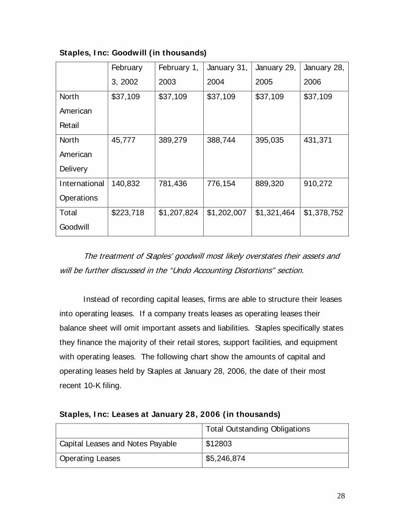
goodwill and intangibles with indefinite lives should be written off. The following
chart shows the steady increases in goodwill since the adoption of SFAS No. 142
on February 3, 2002.
28
Staples, Inc: Goodwill (in thousands)
February
3, 2002
February 1,
2003
January 31,
2004
January 29,
2005
January 28,
2006
North
American
Retail
$37,109 $37,109 $37,109 $37,109 $37,109
North
American
Delivery
45,777 389,279 388,744 395,035 431,371
International
Operations
140,832 781,436 776,154 889,320 910,272
Total
Goodwill
$223,718 $1,207,824 $1,202,007 $1,321,464 $1,378,752
The treatment of Staples’ goodwill most likely overstates their assets and
will be further discussed in the “Undo Accounting Distortions” section.
Instead of recording capital leases, firms are able to structure their leases
into operating leases. If a company treats leases as operating leases their
balance sheet will omit important assets and liabilities. Staples specifically states
they finance the majority of their retail stores, support facilities, and equipment
with operating leases. The following chart show the amounts of capital and
operating leases held by Staples at January 28, 2006, the date of their most
recent 10-K filing.
Staples, Inc: Leases at January 28, 2006 (in thousands)
Total Outstanding Obligations
Capital Leases and Notes Payable $12803
Operating Leases $5,246,874
29
Staples’ also attempts to differentiate themselves from their competitors
by offering an “easy” shopping experience. In order to do so Staples rearranged
all of their North American stores to a customer friendly layout, called the dover
format. The layout opened the interior of the store to give the customer a better
view of Staples’ extensive product array. To account for these improvements,
Staples capitalizes and amortizes these costs in the leasehold improvements
account.
Staples has an ample amount of accounting flexibility when accounting for
advertising costs, goodwill, and leases. The accounting flexibility they have help
management manipulate and manage their reported numbers on their financial
statements and reports.
Evaluation of Actual Accounting Strategy
When evaluating the actual accounting strategy of a firm, it is important
to analyze the accounting policies relative to other leading competitors within the
same industry. It is also critical to relate these accounting strategies to a firm’s
key success factors, which are the most apparent value additives to a firm.
Because Staples, Office Depot, and Office Max possess many similar key success
factors, they do, for the most part, implement similar accounting strategies. In
the following paragraphs, we will identify Staples’ actual accounting strategies of
its key success factors as well as relate them to the accounting strategies of
other leading firms within the industry
Staples’ management has chosen to establish a mixture of aggressive and
conservative accounting policies. For example, Staples’, Office Depot, and Office
Max normally expense advertising costs, but each company has chosen to
capitalize the costs of catalog production, which totaled $28.4 million in 2005
and $30.8 million in 2006. This is an aggressive accounting practice because it
hides advertising expenses in the company’s assets which ultimately increase net
income.

30
Staples and Office Max both take an aggressive stance when it comes to
goodwill impairment. Neither company has recognized an impairment expense
since 2001 which raises a red flag because the assets of both companies might
be overstated. “Managers can use their reporting judgment to delay write downs
on the balance sheet and avoid showing impairment charges in the income
statement” (Palepu, 4-8). The affect of not impairing goodwill each year
increase Staples’ assets by billions of dollars. At the beginning of 2003, Staples
had $1,207,824,000 worth of goodwill. This goodwill was not impaired at the
end of the year, therefore; the assets were overstated and expenses were
understated by a significant amount.
All of the competitors in the office supply superstore industry tend to
avoid capital leases and, instead, expense them as operating leases. For
example, on January 28, 2006 Staples recorded total outstanding lease
obligations amounting to $12,803,000 of capital leases and notes payable, and
$5,246,874,000 of operating leases. This type of aggressive accounting policy
excludes vital lease assets and liabilities from the balance sheet, understating
assets and liabilities.
Overall, the office supplies superstore industry is one that uses
moderately aggressive accounting policies. While Staples does employ some
conservative practices, for the most part, its accounting policies lean more
towards the aggressive side of the spectrum. When compared to Office Depot
and Office Max, however, Staples has accounting policies that are slightly more
conservative than the industry norm.
Quality of Disclosure
The quality of disclosure accounts for the manager’s ability to accurately
disclose information which tells the true story of what is going on in their firm. In
looking at the qualitative disclosure, we will analyze the managers of Staples’
discussion on their business strategy, footnotes explaining accounting policies, its
current performance, and its segment disclosure. We will also conduct a
31
quantitative disclosure using ratios to analyze the firm’s trends and trends within
the industry to see if the firm is overvaluing or undervaluing numbers to make
certain aspects of its business look better than it might actually be.
The quality of disclosure in regards to the business strategy is normally
found in the letter to the shareholders. The business strategy should convey
current industry conditions, the company’s competitive positions, and
management’s plans for the future. Staples provided a letter to the shareholders
along with a business strategy section in the beginning of the 10-k. The letter to
the shareholders informed the readers of Staples’ increase in sales, earnings per
share increase, and an all time high operating margin. It focused mainly on what
it had done over the past year in regards to sales, growth, customer services,
brand development, and supply chain improvements. It did not look at the
future, not did it really give a good analysis of its competitive position. However,
the business strategy section of the 10-k did explain to the shareholders the
company’s competitive position and plans for the future.
The footnotes for a company should explain key accounting policies and
the logic behind them. If any of the policies are different from industry norms,
they need to be explained in the footnotes so that outsiders may have an
explanation of why the balance of numbers might be off. When looking at
Staples’ Footnotes it is apparent that they have adequately explained their key
accounting policies and assumptions. Staples includes information on where they
derived their numbers to formulate their financial statements.
The adequacy with which management discusses its current performance
is a chance for management to relay why certain events took place over the year
or why certain numbers changed in relation to the past. In analyzing their
discussion, we found that Staples did explain why certain numbers changed. For
example, interest income increased to $56.8 million from $39.9 million in the
previous year. In the management’s discussion, they explained that this increase
was due in part to “an increase in interest rates, partially offset by a reduction in

32
outstanding borrowings. Interest expense was also impacted by our November
2004 repayment of 150 million Euro Notes.”(Staples, 10-k)
The Quality of segment disclosure should provide information about how
the firm is divided into product segments and geographic segments. The
information that Staples has disclosed in their segment report gives us details
about their performance. “Staples has three reportable segments: North
American Retail, North American Delivery and International Operations.”
(Staples, 10-k)The information about each segment is broken down into how the
performance is measured by each one. Financial statements are also included to
compare each segments significant accounts and balances. These consolidated
financial statements provide sufficient information to assess staples overall
performance in comparison to their main accounting policies.
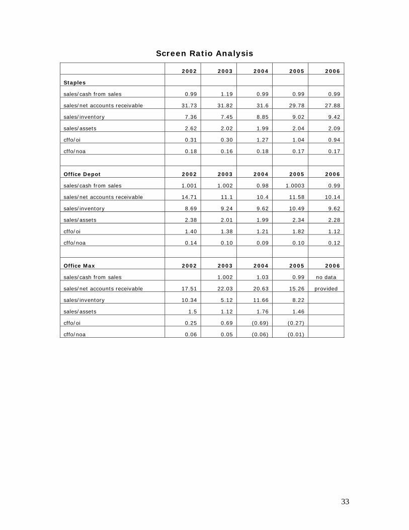
Screen Ratio Analysis will be discussed in the following paragraphs. The
ratios in the table below are core sales and expense diagnostics which help
analysts to see if a company is manipulating its accounting numbers. The
following ratios were not found and will not be discussed due to inadequate
amounts of information: sales/unearned revenues, sales/warranty liabilities, total
accruals/change in sales, pension expense/selling, general, and administrative
costs(SG&A), and other employment expenses/SG&A.
33
Screen Ratio Analysis
2002 2003 2004 2005 2006
Staples
sales/cash from sales 0.99 1.19 0.99 0.99 0.99
sales/net accounts receivable 31.73 31.82 31.6 29.78 27.88
sales/inventory 7.36 7.45 8.85 9.02 9.42
sales/assets 2.62 2.02 1.99 2.04 2.09
cffo/oi 0.31 0.30 1.27 1.04 0.94
cffo/noa 0.18 0.16 0.18 0.17 0.17
Office Depot 2002 2003 2004 2005 2006
sales/cash from sales 1.001 1.002 0.98 1.0003 0.99
sales/net accounts receivable 14.71 11.1 10.4 11.58 10.14
sales/inventory 8.69 9.24 9.62 10.49 9.62
sales/assets 2.38 2.01 1.99 2.34 2.28
cffo/oi 1.40 1.38 1.21 1.82 1.12
cffo/noa 0.14 0.10 0.09 0.10 0.12
Office Max 2002 2003 2004 2005 2006
sales/cash from sales 1.002 1.03 0.99 no data
sales/net accounts receivable 17.51 22.03 20.63 15.26 provided
sales/inventory 10.34 5.12 11.66 8.22
sales/assets 1.5 1.12 1.76 1.46
cffo/oi 0.25 0.69 (0.69) (0.27)
cffo/noa 0.06 0.05 (0.06) (0.01)

34
O U T P U T
Sales/ Cash From Sales
0
0.2
0.4
0.6
0.8
1
1.2
1.4
2002 2003 2004 2005 2006 Year
Staples
Office Depot
Office Max
Revenue Diagnostics
Over the past five years, Staples ratio of cash to cash from sales has
lingered right around 1 with .99 being a common ratio outcome. This means that
Staples is collecting roughly $0.99 in cash from every sale. Their ratio shot above
the rest of the industry in 2003, but has stabilized in the past three years to
average out with the rest of the industry. Office Depot and Office Max also have
sales to cash from sales ratio at 1. This indicates that the industry as a whole is
collecting cash from sales at relatively the same rate. This would lead us to
believe that the majority of sales in the office supply industry are cash sales.

35
The ratio that divides sales by net accounts receivables has dropped over
the past five years indicating Staples is not collecting their cash receivables. It is
currently at its lowest point from the last five years at 27.88. Although its
receivable turnover is higher than the other two competitors, we still question
why the receivables turnover is decreasing. These two ratios, cash divided by
cash from sales and cash divided by net accounts receivable, should move in the
same direction. However, our ratio of cash divided by cash from sales is
stabilizing while cash divided by net accounts receivables is declining. This would
possibly raise a red flag, but Staples can account for this difference in its 10-K
notes to consolidated financial statements. Staples receivables consist of trade
and non-trade receivables. Trade receivables are receivables from the sale of
goods or services on credit. Trade receivables make up for the majority of
account receivables at $444.8 million. “Concentrations of credit risk with respect
to trade receivables are limited due to Staples large number of customers and
their dispersion across many industries and geographic regions.” (Staples, 10-k)
This indicates that their majority sales are collectable which is why the cash to
cash from sales ratio are at .99. The reason the receivables turnover ratio is
Sales/ Net Accounts Receivable
0
5
10
15
20
25
30
35
2002 2003 2004 2005 2006
Year
Out
put Staples
Office DepotOffice Max
36
declining is because of the non-trade receivables which are increasing and
currently account for $148.3 million. Non-trade receivables are receivables from
things other than sale of services or goods. Staples includes this to be “vendors
under various incentive and promotional programs”. (Staples,10-k) This increase
in receivables overall is why the ratio has declined.
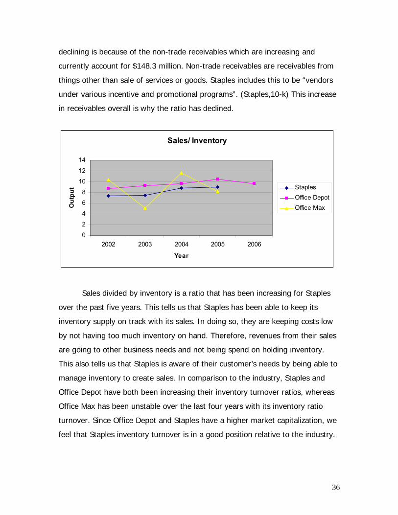
Sales divided by inventory is a ratio that has been increasing for Staples
over the past five years. This tells us that Staples has been able to keep its
inventory supply on track with its sales. In doing so, they are keeping costs low
by not having too much inventory on hand. Therefore, revenues from their sales
are going to other business needs and not being spend on holding inventory.
This also tells us that Staples is aware of their customer’s needs by being able to
manage inventory to create sales. In comparison to the industry, Staples and
Office Depot have both been increasing their inventory turnover ratios, whereas
Office Max has been unstable over the last four years with its inventory ratio
turnover. Since Office Depot and Staples have a higher market capitalization, we
feel that Staples inventory turnover is in a good position relative to the industry.
Sales/ Inventory
0
2
4
6
8
10
12
14
2002 2003 2004 2005 2006
Year
Out
put Staples
Office DepotOffice Max
37
Expense Diagnostics
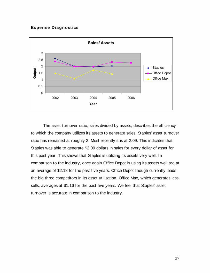
The asset turnover ratio, sales divided by assets, describes the efficiency
to which the company utilizes its assets to generate sales. Staples’ asset turnover
ratio has remained at roughly 2. Most recently it is at 2.09. This indicates that
Staples was able to generate $2.09 dollars in sales for every dollar of asset for
this past year. This shows that Staples is utilizing its assets very well. In
comparison to the industry, once again Office Depot is using its assets well too at
an average of $2.18 for the past five years. Office Depot though currently leads
the big three competitors in its asset utilization. Office Max, which generates less
sells, averages at $1.16 for the past five years. We feel that Staples’ asset
turnover is accurate in comparison to the industry.
Sales/ Assets
0
0.5
1
1.5
2
2.5
3
2002 2003 2004 2005 2006
Year
Out
put Staples
Office DepotOffice Max

38
CFFO/ OI
-1
-0.5
0
0.5
1
1.5
2
2002 2003 2004 2005 2006
Year
Out
put Staples
Office DepotOffice Max
The cash flow from operations (cffo) to operating income (oi) ratio for
Staples has fluctuated around 1 for the past three years. Staples had operating
income as a line item on its income statements filed for 2006, 2005, and 2004.
However, it did not have it as a line item for the reports filed in 2003 and 2002.
This is why the ratio jumps from 0.30 to 1.27 in the filing of 2004. We had to
compute operating income for the 2003 and 2002 filings. Staples ratio for the
past three years is a better comparison to Office Depot, its main competitor,
because we did not have to compute their operating income either. Staples last
filing in 2006 tells us that $0.94 of every dollar of cash flow from operations
results in operating income. Office Depot has remained along 0.2 and Office Max
has been very unstable in its cash flow from operations to operating income
ratios. The graph shows that the companies in the office supply industry have
been inconsistent in their cash flow from operations to operating income. It also
tells us that the industry as a whole is not generating enough operating income
to support cash flows. Noting that we can compare Staples past three years with
the Office Depot, we see that their ratios were very similar in 2004, and in 2005
and 2006 Office Depot has been declining in its ratios and Staples has been
inconsistent. We would need a few more years to see if the industry is just trying

39
to stabilize itself or if there are actual real problems for this industry in profiting
from its operations.
Cash flow from operations divided by net operating assets tells us how
well a company utilizes its assets to generate cash flows. Once again Staples’
ratio has remained stable over the last five years at roughly .172. It leads the
industry since Office Depot’s ratio has been at about .11, and Office Max has
been unstable in this ratio as well. This shows that Staples is utilizing its
operating assets more effectively than its two main competitors and is able to
generate cash flows from them.
Identifying Potential “Red Flags”
When reviewing a firm’s financial statements it is important to be aware of
abnormal and suspicious behavior and information. These “red flags” arise
though a firm’s accounting strategies within their flexibility limitations. They
highlight the need to re-examine accounting procedures and outcomes to
determine if the company overvalued or undervalued its numbers to make the
shareholders believe the company is doing better than it actually is. We believe
CFFO/ NOA
-0.1
-0.05
0
0.05
0.1
0.15
0.2
2002 2003 2004 2005 2006
Year
Out
put Staples
Office DepotOffice Max

40
that the ratios including sales divided by cash from sales, sales divided by net
account receivables, sales divide by inventory, sales divided by assets, cash flow
from operations (cffo), and cash flow from operations divided by net operating
assets (noa) do not raise any potential red flags for Staples.
The treatment of goodwill by firms has significantly changed since the
implementation of SFAS No. 142. Since Staples adopted the accounting policy
on February 3, 2002 they have acquired six businesses globally including a total
increase in goodwill of $1,155,034,000. The problem is, since the change in
accounting policy, Staples has not accounted for any impairment charges nor
written off any goodwill. This aggressive accounting behavior leads to an
overstatement of intangible assets and an understatement of impairment
expenses.
Staples also uses aggressive accounting strategies with advertising costs.
Staples normally expenses advertising costs, but capitalizes and amortizes
catalog costs over the life of the catalog. While the amounts of catalog costs are
relatively low, they still raise concerns over Staples’ accounting strategy, because
they are assuming all these catalogs are assets and will provide future economic
benefits. Capitalized catalog costs amounted to $30,800,000 at January 29,
2005 and $28,400,000 at January 28, 2006. We conclude, these distortions are
not significant enough to be undone due to their low relative magnitude, but
they still raise concern and should have been recognized as an expense.
Treatment of leases plays a significant role on firms’ financial statements.
Staples structures their leases as mainly operating leases to finance their retail
stores, support facilities, and equipment, while using capital leases for the
remainder. Staples’ capital leases at January 28, 2006 totaled $12,803,000 while
their operating leases total $5,246,874,000. Treating leases as operating leases
greatly understates lease asses and lease liabilities, thus having a detrimental
impact on the balance sheet.

41
We did not find any “red flags” associated with our ratio analysis. This
may be a result of Staples’ use of aggressive accounting strategies and number
manipulations.
Undo Accounting Distortions
The red flags stated in the “Potential Red Flags” section of this document
skewed numerical figures to make the firm appear more profitable. It is
important when valuing Staples to undo these accounting distortions in order to
truthfully state the firm’s financial position.
As stated previously, Staples leases a majority of its new properties by
way of operating leases.
Staples’ Operating Lease Obligations:
Operating Leases
Year FV i = 7% PV 1 $617,021 0.935 $576,655.14 2 $593,176 0.873 $518,102.89 3 $558,355 0.816 $455,784.00 4 $526,981 0.763 $402,031.28 5 $491,310 0.713 $350,297.24 6 $492,006 0.666 $327,844.37 7 $492,006 0.623 $306,396.61 8 $492,006 0.582 $286,351.97 9 $492,006 0.544 $267,618.66
10 $492,006 0.508 $250,110.90 $3,741,193.07
The table above shows the present value of Staples’ future payments on its
operating leases. We used ten years because when assuming a 20 year
maturity, the payments decreased from year 5 to years 6-20 by about $300
million dollars. By assuming a ten year maturity, we kept the remaining
payments (Years 5 – 10) fairly close to the payments in the first 5 years. This
effect is somewhat of a tradeoff between having a drastic decrease in payments

42
after 5 years which would be hard to justify in the financial statements and
paying off the leases much faster due to large payments. We assumed a 7%
discount rate because that is about the industry standard. From the table, it can
be determined that Staples is hiding about $3.7 billion worth of liabilities.
To undo this distortion, Staples should increase it leased assets and lease
liabilities by $3.7 billion. Staples should also recognize a depreciation expense
each year of roughly $374 million ($3741193.07/10 years). The affect of this
large expense recognition would ultimately decrease net income, but accurately
state Staples’ assets and liabilities.
Assets:
Leased Assets (Land and Buildings): +$3.7 billion
Liabilities:
Lease Liabilities (Capital Leases): +$3.7 billion
Staples’ also distorted accounting policies when dealing with its
impairment of goodwill. As stated previously, Staples has not evaluated goodwill
for impairment since 2001. By not doing so, the company is overstating its
assets considerably. Even though goodwill is not amortized, we believe an
accurate assumption would be to amortize it over 10 years. This amortization
expense should be similar to the amount that should have been impaired by
Staples’ management at the end of each year. In doing so, Staples would
decrease its assets to portray a truthful figure. Since total goodwill equals
$1,378,752,000, we believe it is fair to amortize this amount over 10 years at a
rate of $137,875,200 per year. This will decrease the current value of goodwill
to zero over ten years because we believe the goodwill already acquired will
have lost its value.

43
Ratio Analysis and Forecasting Financials
Financial Analysis
Financial Analysis is a very important part of valuing a firm. We use the
company’s balance sheets, income statements, and statements of cash flows to
analyze the company’s plans and the performance of the firms and corporate
managers. We do this analysis through the use of ratios in which we compute for
Staples and its competitors. This allows us to make comparisons and note
trends.
Ratio Analysis
In valuing a firm, you must perform a ratio analysis. This provides you
with a way to relate different line items of the financial statements and then
assess those relationships. A cross-sectional comparison allows you to examine
the ratios of your company to its competitors. There are three main groups of
ratios: liquidity, profitability, and capital structure. We will analyze these ratios
for Staples, Office Depot, and Office Max and compare them against each other.
Trend (Time Series) Analysis/ Cross Sectional Analysis
We will begin with the liquidity ratios. These ratios include the current
ratio, quick-asset ratio, inventory turnover, days inventory turnover, receivables
turnover, days receivables turnover, and working capital turnover. Liquidity ratios
look at the amount of cash-equivalence in a company’s assets and its ability to
turn assets into cash to meet financial obligations. After computing the ratios for
Staples and its competitors, we will now analyze these ratios and identify any
trends within Staples as well as within the industry. We will begin with the
current ratio which is found by dividing current assets by current liabilities.

44
Liquidity Ratios
Current Assets: Current Assets/Current Liabilities
2001 2002 2003 2004 2005 2006
Staples 1.51 1.25 1.64 1.72 1.67 1.59
Office Depot 1.61 1.57 1.51 1.43 1.16
Office Max 1.23 1.31 1.75 1.22 1.37
The current ratio is an analysis of the amount of current assets a company
has to cover its current liabilities. Current assets consist of cash and cash
equivalents, short term investments, net receivables, net merchandise
inventories, deferred income tax assets, and prepaid expenses. Current liabilities
consist of accounts payable, accrued expenses and other current liabilities, and
debt maturing within one year. When reading this ratio, you would state that for
every dollar of current liabilities, the company has an amount of current assets to
cover those liabilities. Staples, for example, had a current ratio in 2006 that
shows that for every dollar of current liabilities, they had $1.59 in current assets
to cover those liabilities. A ratio over one suggests that the company has the
ability to pay its short term liabilities with its current assets. A ratio under one
does not necessarily mean the company will go bankrupt, it just shows that
company is not in good financial health. The higher the ratio is, the more liquid
its current assets and therefore it has a better ability to meet short term
obligations. However, if the current ratio is too high, that tells us that the firm is
not utilizing its assets efficiently.

45
Current Asset Ratio
1
1.1
1.2
1.3
1.4
1.5
1.6
1.7
1.8
2001 2002 2003 2004 2005
years
outp
ut StaplesOffice DepotOffice MaxIndustry Avg.
Staples has an average over the past six years of 1.56 with its high being
at 1.72 and its low at 1.25. These tell us that Staples is using its assets efficiently
and has the ability to cover its short term debt. Its current assets have been
steadily increasing at roughly 80% to 90% and its current liabilities have not
been increasing as consistently. This is why its current ratio has varied over the
past six years. Office Depot and Office Max are also both utilizing their assets
efficiently and have the ability to cover their short term debt.
The quick asset ratio is a measure of how easily a company can be
liquidated. This tells us how credit-worthy a company is. Then companies are
rated as being strong or weak by financial institutions.

46
Quick Asset Ratio: cash + securities + A/R / Current Liabilities
2001 2002 2003 2004 2005 2006
Staples 0.46 0.44 0.41 0.67 0.63 0.62
Office Depot 0.83 0.88 0.86 0.78 0.56
Office Max 0.46 0.35 1.02 0.42 0.55
Industry Average 0.58 0.56 0.76 0.63 0.58
The quick asset ratio gives us a better idea of if a company has the ability
to cover its short term obligations. This is because it does not include inventory
like the current ratio does. Inventory is hard to guarantee that it will be liquid
because you can not be sure that you can sell your inventory at the market price
at any given time. A low quick ratio indicates an efficient use of current assets.
Staples has been operating fairly efficiently based on the given ratios. However,
over the past three years the ratios have increased. This is just due to an
increase in quick assets.
Quick Asset Ratio
0.00
0.20
0.40
0.60
0.80
1.00
1.20
2001 2002 2003 2004 2005
years
outp
ut
StaplesOffice DepotOffice MaxIndustry Avg.
In comparison with its competitors, Staples has fallen below the industry
average until 2004. This also shows that Staples has been the most efficient in

47
the use of its assets until 2005. Office Depot has been the most inefficient with
its quick asset ratio staying above industry average until recently in 2005. Office
Max has been very inconsistent in using its assets efficiently. Staples ability to
keep a low quick asset ratio consistently shows that management has been
effectively utilizing their assets.
Inventory Turnover: Cost of Goods Sold/Inventory
2001 2002 2003 2004 2005 2006
Staples 5.60 5.56 6.46 6.45 6.74 6.75
Office Depot 6.14 6.35 6.61 7.27 6.63
Office Max 8.36 4.12 8.99 6.11 6.09
Industry Average 6.70 5.34 7.35 6.61 6.49
Inventory turnover is a measure of how many times a firm sells and
replaces its inventory over a given time period. It is found by taking cost of
goods sold and dividing it by inventory. A low turnover rate may indicate
overstocking, problems in the marketing effort or product line, or a decline in
interest by the consumers for that product. A high turnover rate may indicate
inadequate inventory levels. The appropriate inventory level depends on the
business that the firm is within. According to www.retailowner.com, Staples
inventory should be about 6 to 7 turns. Staples inventory turnover rate averages
at about 6 turns. This tells us that Staples is selling its stock of inventory and
restocking on average six times a year. Staples, therefore, is generating high
profits.

48
Inventory Turnover
3
4
5
6
7
8
9
10
2001 2002 2003 2004 2005
years
outp
ut
StaplesOffice DepotOffice MaxIndustry Avg.
As you can see from the graph, Staples’ inventory turnover seems to be
on the same track as the industry average, sometimes dipping just a little below
or above the average. Office Depot seems to be following that trend as well.
These are the two main competitors in this industry, so it leads us to believe that
Staples’ inventory levels are in line with customer demand and that the product
line is effective. Office Max’s inventory turnover is inconsistent due to their sales
and inventory rates. In 2004, their sales spiked unexpectedly, and therefore they
overstocked for 2005. This caused their irregular ratios. Staples increasing
inventory turnover can be linked to their marketing efforts. They launched the
easy brand promise in 2003 and “the easy button” in 2005. With both of these
efforts, they increased their sales which increased their supply of inventory and
therefore their inventory turnover ratio. Staples continues to grow and
management has done a good job at keeping inventory levels in sync with their
sales.

49
Days Supply Inventory Turnover: 365/Inventory Turnover
2001 2002 2003 2004 2005 2006
Staples 65.19 65.6 56.51 56.55 54.19 54.04
Office Depot 59.4 57.49 55.24 50.22 55.05
Office Max 43.67 88.62 40.59 59.74 59.90
Industry Average 56.09 70.57 50.78 55.50 56.38
Days supply inventory turnover ratio tells us how many days it takes for a
firm to turnover its inventory. It is found by dividing 365 days by the inventory
turnover rate. A low days supply of inventory turnover is desirable because it
means that the company is not holding inventory in storage for long periods of
time. Staples has been decreasing its days supply inventory turnover over the
past six years. This indicates that Staples’ is managing its inventory in relation to
its sales more effectively. They are not only turning over their inventory at a
faster rate, but they are also turning over their days supply inventory at a faster
rate. This shows that Staples is generating higher profits, getting inventory out
of its stores faster, and managing their inventory levels better.
Days Supply Inventory Turnover
30
40
50
60
70
80
90
100
2001 2002 2003 2004 2005
years
oupu
t
StaplesOffice DepotOffice MaxIndustry Avg.

50
Compared to its main competitors, Staples seems to be aligning with the
industry. Office Depot leads the industry with consistently having a lower days
supply inventory turnover rate. Office Max once again is inconsistent with its
ratios. Staples declining days supply inventory ratio tells us several things. It says
that they are able to better use their assets. We know this because the lower the
days supply turnover rate, the less amount of days that inventory is actually
staying in storage. This means that Staples is spending less money on their
holdings of inventory which means they are utilizing their assets better. Their
turnover rate also tells us that they have significant relations with their suppliers.
This would imply that due to their decreasing days supply turnover rate and
increasing brand recognition that Staples holds bargaining power over its
suppliers. This is beneficial to Staples’ sales and cost of goods sold which are
apart of their inventory turnover ratio. This is also important to their key success
factors in which they compete on cost. By hold bargaining power over their
suppliers they are able to buy their products at a lower cost, thus in turn able to
sell it a lower price.
Receivables Turnover: Sales/Accounts Receivable
2001 2002 2003 2004 2005 2006
Staples 31.73 31.82 31.6 29.78 27.88 25.2
Office Depot 10.40 7.63 7.14 8.02 10.14
Office Max 17.48 14.36 20.63 15.26 15.94
Industry Average 19.87 17.94 19.79 17.69 17.99
Accounts receivables turnover is found by dividing sales by accounts
receivables. “This ratio tells us the number of times accounts receivables are paid
and reestablished during the accounting period. The higher the turnover, the
faster the business is collecting its receivables and the more cash the client
generally has on hand (www.missouribusiness.net).” It measures a firm’s
effectiveness in extending credit and collecting debt. Staples has an average

51
turnover rate at 29.67 turns. This indicates to us that Staples is effective in
collecting its accounts receivables and probably operates on a cash basis. We
can confirm this when looking at the balance sheets for Staples. Over the past
six years, Staples cash account is a lot higher compared to its accounts
receivables.
Receivables Turnover
0
5
10
15
20
25
30
35
2001 2002 2003 2004 2005
years
outp
ut
StaplesOffice DepotOffice MaxIndustry Avg.
As you can see from the graph, Staples leads the industry in receivables
turnover. This shows us that Staples is managing its accounts receivables better
than the other two companies. Office Depot has the lowest receivables turnover
rates from 2001 to 2005 which means that they are not collecting on their
receivables in relation to their sales rates. Office Max stays right about the
industry average indicating that they are collecting on their receivables with
enough efficiency. Staples recent decline in their ratios is due to an increase in
accounts receivables.

52
Days Sales Outstanding: 365/Receivables Turnover Ratio
2001 2002 2003 2004 2005 2006
Staples 11.50 11.47 11.55 12.26 13.09 14.49
Office Depot 24.08 32.85 35.09 31.50 36.00
Office Max 20.88 25.42 17.69 23.92 22.9
Industry Average 18.82 23.25 18.11 22.56 24.00
Days Sales Outstanding tells us how many days it takes the firm to collect
their accounts receivables. A lower ratio is preferable because it indicates that
the company is collecting their receivables at a fast rate. Staples ratio averages
at 12.39 days for the past six years. This means that on average they collected
their accounts receivables 12 days after the purchase date. This is a very good
rate for Staples.
Days Sales Outstanding
05
10152025303540
2001 2002 2003 2004 2005
years
outp
ut
StaplesOffice DepotOffice MaxIndustry Avg.
Staples, as you can see from the graph, leads the industry with the lowest
days sales outstanding ratios. This, once again, is indicative that they are taking
the least amount of days to collect cash from their accounts receivables. Office
Depot has the highest days sales outstanding ratios. This, which correlates with

53
their receivables turnover ratio, further proves that Office Depot is struggling to
collect cash on their accounts receivables. Their receivables account is increasing
and they are taking longer to cash in on the account. Office Max seems to stay
within the industry average just like the receivables turnover ratio. Both their
cash and receivables have increased over the years, however their sales have
not been as steady. In most recent years their sales have declined. This is why
Office Max’s ratios have not been consistent. According to Staples annual 10-k
report in 2006, the reason that they are able to collect on their accounts is
because they have a high customer base spread out internationally and within
different industries. We agree with this statement as well as from the ratios we
see that Staples has a lot of cash basis transactions.
Working Capital: sales/working capital
2001 2002 2003 2004 2005 2006
Staples 13.31 21.39 9.57 9.12 9.66 11.05
Office Depot 9.33 9.51 10.24 13.45 30.94
Office Max 30.61 13.5 9.59 25.89 15.79
Industry Average 17.75 14.80 9.80 16.15 18.80
Working capital is a ratio that measures how many dollars of working
capital generate sales. It is found by dividing sales by working capital. Working
capital is found by subtracting current liabilities from current assets. A higher
working capital turnover is preferred because it means you are generating sales
from your working capital. Staples working capital has decreased and has been
inconsistent over the past six years. Its high was in 2002 at 21.39. It declined
from 2003 to 2005, and has increased again for this past annual report. The
reason behind the decline was due to an increasing working capital that did not
match the increase in sales. They were both increasing, but working capital was
increasing at a faster rate. For this last annual report, Staples working capital
ratio is at 11.05 which is an increase from 2005. This means that for 2006,

54
Staples generated $11.05 in sales off of every dollar in working capital. As
compared with Office Depot, who in its last annual report for 2005 was
generating $30.94 in sales off of every working capital dollar. Staples’ managers
will need to change their use of assets considering that Office Depot makes over
double off of their working capital dollars than Staples.
Working Capital
0
5
10
15
20
25
30
35
2001 2002 2003 2004 2005
years
outp
ut
StaplesOffice DepotOffice MaxIndustry Avg.
As you can see from the graph, none of these companies have been very
stable in their working capital ratios. This tells us that the companies are
struggling to utilize their assets effieciently and generate profits off of them in a
consistent manner. Office Depot has the best working capital ratios. They are
increasing with each year. This is due to a decrease in their working capital and
increase in sales. Office Max has once again been inconsistent in managing its
assets. Staples decline in compared to the industry means that its managers are
not utilizing its working capital assets as effectively as compared to its
competitors.
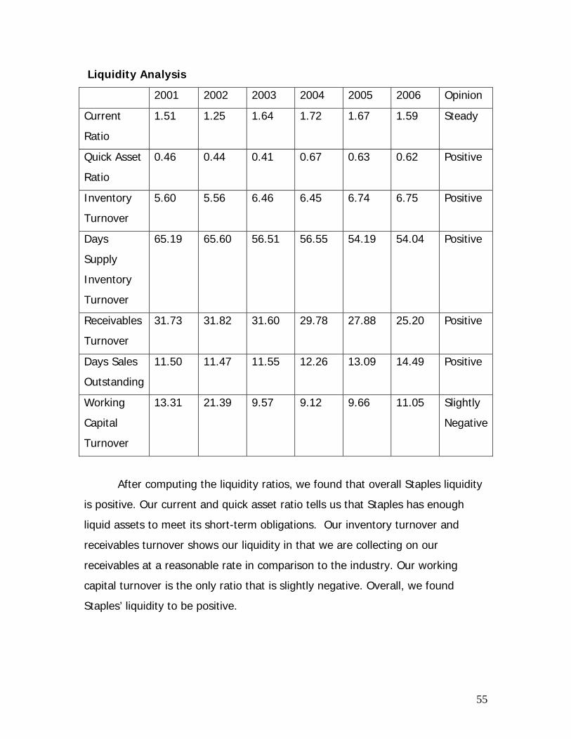
55
Liquidity Analysis
2001 2002 2003 2004 2005 2006 Opinion
Current
Ratio
1.51 1.25 1.64 1.72 1.67 1.59 Steady
Quick Asset
Ratio
0.46 0.44 0.41 0.67 0.63 0.62 Positive
Inventory
Turnover
5.60 5.56 6.46 6.45 6.74 6.75 Positive
Days
Supply
Inventory
Turnover
65.19 65.60 56.51 56.55 54.19 54.04 Positive
Receivables
Turnover
31.73 31.82 31.60 29.78 27.88 25.20 Positive
Days Sales
Outstanding
11.50 11.47 11.55 12.26 13.09 14.49 Positive
Working
Capital
Turnover
13.31 21.39 9.57 9.12 9.66 11.05 Slightly
Negative
After computing the liquidity ratios, we found that overall Staples liquidity
is positive. Our current and quick asset ratio tells us that Staples has enough
liquid assets to meet its short-term obligations. Our inventory turnover and
receivables turnover shows our liquidity in that we are collecting on our
receivables at a reasonable rate in comparison to the industry. Our working
capital turnover is the only ratio that is slightly negative. Overall, we found
Staples’ liquidity to be positive.

56
Profitability Ratios
Gross Profit Margin (%): Gross Profit/Sales
2001 2002 2003 2004 2005 2006
Staples 23.92 25.38 26.98 28.41 28.52 28.60
Office Depot 29.36 31.35 31.38 30.76 31.10
Office Max 19.04 19.65 22.88 25.64 27.18
Industry Average 24.11 25.46 27.08 28.27 28.93
Gross Profit Margin tells us how efficiently a company uses its materials
and labor in the production process. It is a measure of the amount of profit left
over after cost of goods sold. A high gross profit ratio is favorable because it
means that the company is generating profits after cost of goods sold is
subtracted out. Over the past six years, the gross profit margin for Staples has
increased from 23.92 to 28.60. This tells us that Staples has become more
efficient over the past six years in their production process. This efficiency has
come from several different factors. “Gross profit as a percentage of sales was
28.6% for fiscal 2006, 28.5% for fiscal 2005, and 28.4% for fiscal 2004 (Staples
10-k).” Gross profit on its own has been increasing in relation to sales. General
and administrative and operating and selling expenses also have both declined in
relation to sales. All of these things add up to the increase in gross profit margin
over the past couple years.
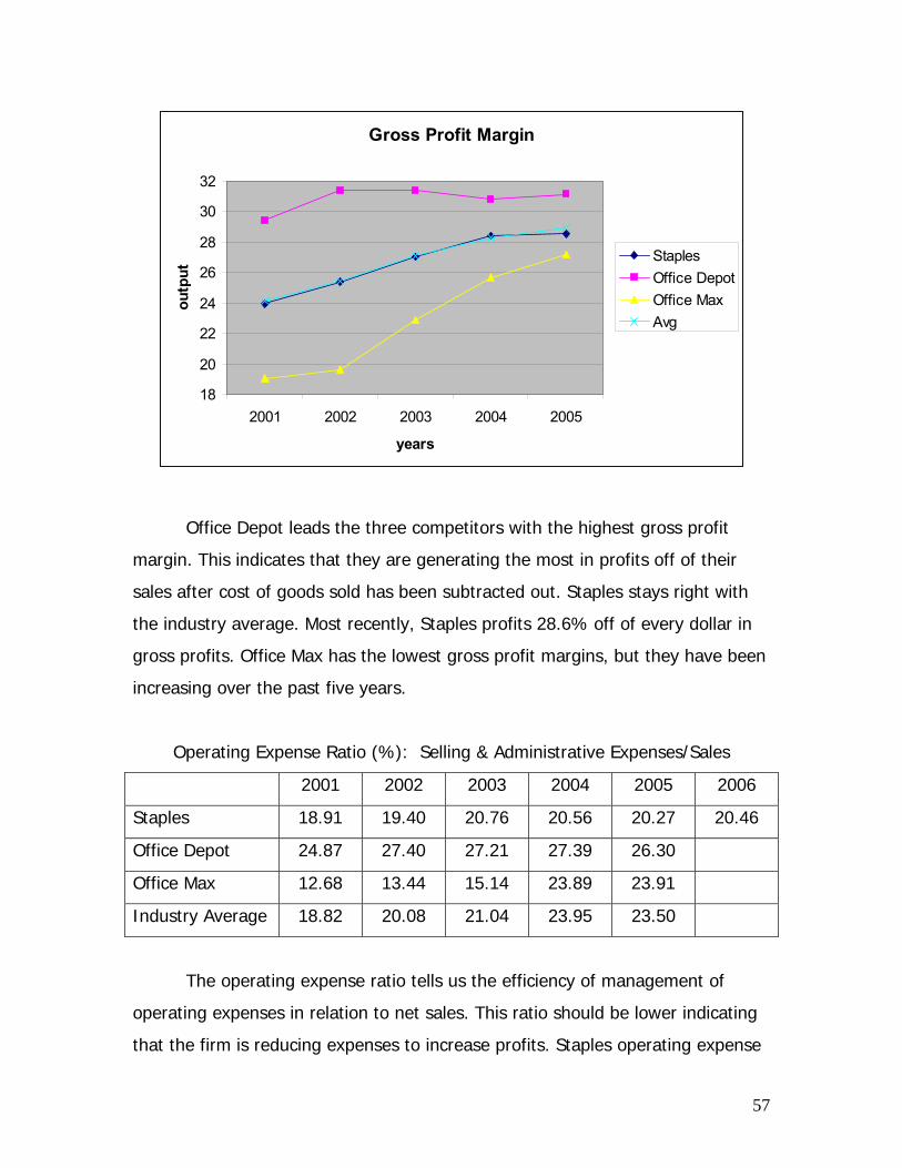
57
Gross Profit Margin
18
20
22
24
26
28
30
32
2001 2002 2003 2004 2005
years
outp
ut
StaplesOffice DepotOffice MaxAvg
Office Depot leads the three competitors with the highest gross profit
margin. This indicates that they are generating the most in profits off of their
sales after cost of goods sold has been subtracted out. Staples stays right with
the industry average. Most recently, Staples profits 28.6% off of every dollar in
gross profits. Office Max has the lowest gross profit margins, but they have been
increasing over the past five years.
Operating Expense Ratio (%): Selling & Administrative Expenses/Sales
2001 2002 2003 2004 2005 2006
Staples 18.91 19.40 20.76 20.56 20.27 20.46
Office Depot 24.87 27.40 27.21 27.39 26.30
Office Max 12.68 13.44 15.14 23.89 23.91
Industry Average 18.82 20.08 21.04 23.95 23.50
The operating expense ratio tells us the efficiency of management of
operating expenses in relation to net sales. This ratio should be lower indicating
that the firm is reducing expenses to increase profits. Staples operating expense

58
ratios are low with an average of 20.06% for the past six years. This shows that
management is doing a good job of keeping their operating expenses low while
still increasing profits.
Office Depot leads the industry in operating expense ratios averaging at
26.63%. This means that they are not managing their operating expenses very
well. Their expenses are high in relation to sales, so they are profiting less from
those sales. Staples’ operating expense ratios align with the industry average
until 2004 where they fall below the industry average. This means that Staples is
continuously working on keeping their expenses low and increasing revenues.
Falling below industry average is actually a good thing, meaning that they are
becoming the leaders of the industry since a lower operating expense ratio is
preferable. Management of Staples is continuously working on keeping their
expenses low and in comparison with the rest of the competition they appear to
be ahead of the game. Office Max was leading the industry with the lowest ratios
until 2004 where it spiked up really high. This is due to a decrease in sales from
previous years.
Operating Expenses
10
15
20
25
30
2001 2002 2003 2004 2005years
output Staples Office DepotOffice MaxIndustry Average

59
Net Profit Margin (%): Net Income/Sales
2001 2002 2003 2004 2005 2006
Staples 2.47 3.85 3.78 4.90 5.19 5.36
Office Depot 2.74 2.21 2.47 1.92 3.44
Office Max 0.15 0.10 1.30 -0.81 1.02
Industry Average 1.79 2.05 2.52 2.00 3.22
Net profit margin measures how much of every dollar is actually retained
as earnings. A higher net profit margin is preferred meaning that the firm is
profitable and that it has very good cost control. Staples’ net profit margin has
increased over the past six years. This indicates that they are controlling costs
and able to hold on to more of every dollar generated in sales. This would also
be another indicator of Staples’ ability to hold bargaining power over their
suppliers. When holding power over their suppliers, they are able to buy their
products from their suppliers at lower costs which is why we see an increase in
their net profit margin. We came to this conclusion because their net income and
sales are increasing together. In the fiscal year of 2006, Staples was collecting
roughly $0.05 on every sales dollar in comparison to 2001 when they collected
roughly $0.02 on every sales dollar.

60
Net Profit Margin
-2
-1
0
1
2
3
4
5
6
2001 2002 2003 2004 2005
years
outp
ut
StaplesOffice DepotOffice MaxIndustry Average
As you can see from the graph, Staples leads the industry in net profit
margin ratios. Office Depot tends to stay right with the industry average, but
more recently has began to increase. This could be due to cost leadership or
their increase in sales. This indicates that the office products industry is growing
and that relationships between buyers and suppliers are being established. Office
Max is inconsistent with their ratios. This tells us that they are having trouble
controlling their costs as well as they have had a recent decline in sales. The
industry as a whole has low net profit margin ratios. This is due to the pricing
strategy of this industry. The office products industry competes on low prices
and the majority of their products are high volume sales. Their main products
are office products such as pens, staplers, copy paper, and printer ink. These are
all products that will be sold in high volume amounts. In selling high volume
products at low costs, your net profit margins will be lower because of the lower
sales price associated with the costs.

61
Asset Turnover
2001 2002 2003 2004 2005 2006
Staples 2.63 2.03 1.99 2.04 2.09 2.16
Office Depot 2.38 2.01 2.1 2.34 2.28
OfficeMax 1.49 1.12 1.73 1.46 1.44
Industry Average 2.17 1.72 1.94 1.95 1.94 2.16
The table above displays the asset turnover ratio over the past five years
for Staples and its competitors. Asset turnover is calculated by taking the sales
of a firm and dividing it by its total assets. This will show us how efficient Staples
is at using its assets to generate sales. With an average of 2.16 over the past
five years, we can see that Staples has a fairly neutral profit margin. Since
Staples owns so many retail stores and also has to keep an extremely large
amount of inventory on hand due to their high demand internet based business,
in turn this inflates the asset denominator. The reason why their ratio was
larger in 2002 and then decreased a somewhat significant amount in 2003 was
because their current assets were high in relevance to their amount of revenue
for the subsequent years.
When looking at the Industry average for the past five years it is clear the
Staples and Office Depot are in the lead, while OfficeMax is once again trailing.
For the entire industry the revenue seems to be strong with a slowly but steadily
increasing ratio.
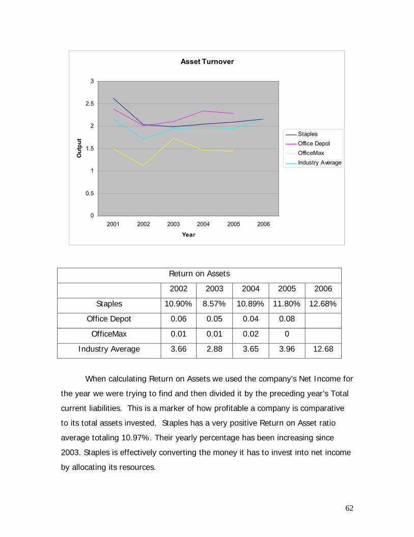
62
Asset Turnover
0
0.5
1
1.5
2
2.5
3
2001 2002 2003 2004 2005 2006
Year
Out
put
StaplesOffice DepotOfficeMaxIndustry Average
When calculating Return on Assets we used the company’s Net Income for
the year we were trying to find and then divided it by the preceding year’s Total
current liabilities. This is a marker of how profitable a company is comparative
to its total assets invested. Staples has a very positive Return on Asset ratio
average totaling 10.97%. Their yearly percentage has been increasing since
2003. Staples is effectively converting the money it has to invest into net income
by allocating its resources.
Return on Assets
2002 2003 2004 2005 2006
Staples 10.90% 8.57% 10.89% 11.80% 12.68%
Office Depot 0.06 0.05 0.04 0.08
OfficeMax 0.01 0.01 0.02 0
Industry Average 3.66 2.88 3.65 3.96 12.68

63
When looking at the Return on Assets Ratio table we can see that Staples
competitors fall extremely far behind. Both Office Depot and OfficeMax’s net
income is far less than their total assets which give them such poor ROA ratios.
This is due to a very low number of investments. The industry average is far off
from all three companies but stays fairly consistent.
Return on Assets
0
2
4
6
8
10
12
14
2002 2003 2004 2005 2006
Year
Out
put
StaplesOffice DepotOfficeMaxIndustry Average
Return on Equity
2002 2003 2004 2005 2006
Staples 21.72 18.44 19.34 20.28 22
Office Depot 0.11 0.12 0.09 0.19
OfficeMax 0.05 -0.02 0.07 0.01
Industry Average 7.29 6.18 6.50 6.83 22.00
When calculating Return on Equity the Net Income is divided by the total
equity of the firm for the previous year. This indicates how much profit the firm
will generate with the money shareholders invested. Looking at Staples ROE
from the years shown in the table above we can see that they have not
produced a steady trend but they are at the highest they have been in five year
with a ratio of 22% for the year 2006.

64
Once again Staples competitors have fallen behind because of such a low
Net Income as the numerator to a inflated shareholder’s equity. From just
looking at these ratios Office Depot and OfficeMax does not appear to be very
profitable.
Return on Equity
-5
0
5
10
15
20
25
2002 2003 2004 2005 2006
Year
Out
put
StaplesOffice DepotOfficeMaxIndustry Average
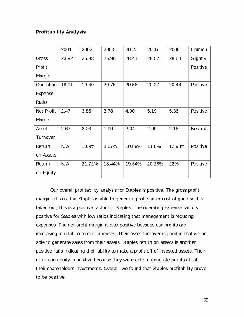
65
Profitability Analysis
2001 2002 2003 2004 2005 2006 Opinion
Gross
Profit
Margin
23.92 25.38 26.98 28.41 28.52 28.60 Slightly
Positive
Operating
Expense
Ratio
18.91 19.40 20.76 20.56 20.27 20.46 Positive
Net Profit
Margin
2.47 3.85 3.78 4.90 5.19 5.36 Positive
Asset
Turnover
2.63 2.03 1.99 2.04 2.09 2.16 Neutral
Return
on Assets
N/A 10.9% 8.57% 10.89% 11.8% 12.98% Positive
Return
on Equity
N/A 21.72% 18.44% 19.34% 20.28% 22% Positive
Our overall profitability analysis for Staples is positive. The gross profit
margin tells us that Staples is able to generate profits after cost of good sold is
taken out; this is a positive factor for Staples. The operating expense ratio is
positive for Staples with low ratios indicating that management is reducing
expenses. The net profit margin is also positive because our profits are
increasing in relation to our expenses. Their asset turnover is good in that we are
able to generate sales from their assets. Staples return on assets is another
positive ratio indicating their ability to make a profit off of invested assets. Their
return on equity is positive because they were able to generate profits off of
their shareholders investments. Overall, we found that Staples profitability prove
to be positive.

66
Capital Structure Ratios
The optimal capital structure for a firm is determined by the risk that it
takes which is entailed within its liabilities. Part of a company’s short and long-
term debt is considered when analyzing capital structure. The capital structure
ratios include the Debt to Equity Ratio, the Time Interest Earned Ratio, and the
Debt Service Margin Ratio.
Debt to Equity Ratio
Year 2001 2002 2003 2004 2005 2006
Staples 0.91 1.03 1.23 1.25 1.28 1.42
Office Depot 1.07 1.19 1.11 1.23 1.52
OfficeMax 2.53 2.17 1.93 2.61 2.13
Industry Average 1.50 1.46 1.42 1.70 1.64 1.42
A company’s debt to equity ratio is what provides and indication of how
many dollars of debt financing the firm is using for each dollar invested by its
shareholders. Staples average amount for every dollar they have invested n
equity over the past five years is $1.19. This tells us that Staples does not
average a large amount of debt. We can see that their debt to equity has been
slightly increasing over the past five years. This could be because Staples has
been growing by opening new stores as well as their Internet based clientele;
therefore inquiring more and more debt.
Compared to Staples competitors, they have the lowest debt to equity
ratio. This tells us that even though they are growing they are not doing so in
such a way that would inquire a large amount of risk. Office Depot is not far
behind which makes them their strongest competitor while OfficeMax is trailing
by over a dollar more. Even though OfficeMax is decreasing their debt it might
not be a good thing. Office Max might be reducing their number of stores which
only puts Staples at an advantage.

67
Debt to Equity Ratio
0.00
0.50
1.00
1.50
2.00
2.50
3.00
2001 2002 2003 2004 2005 2006
Year
Ouu
tput
Staples
Office Depot
OfficeMax
Industry Average Average
Times Interest Earned
Year 2001 2002 2003 2004 2005 2006
Staples 16.83 33.12 25.28 28.23 23.13 30.6
Office Depot 10.37 8.04 7.55 11.16 17.81
OfficeMax 0.01 0.37 2.49 0.29 1.39
Industry Average 9.07 13.84 11.77 13.23 14.11 30.60
To calculate the Time Interest Earned Ratio we take the earnings before
interest and taxes (EBIT) and then divide it by the interest expense. This
indicates how many times Staples can cover its interest charges on a pretax
basis. A ratio of one means that the firm is barely covering its interest expense
through its operating activities; which puts the firm at risk. The larger the ratio
the more room it has to pay their interest expense. The average times interest
earned ratio for Staples over the pas six year equals 26.13. With a ratio that
high, Staples is not putting their firm at risk.

68
When comparing Staples to its competitors we have found that they are
ahead of the game. Office depot’s average times interest earned equals 10.98,
which is far less than half of Staples. OfficeMax’s interest earned is no
competition with an average of 0.91.
Times Interest Earned
0
5
10
15
20
25
30
35
2001 2002 2003 2004 2005 2006
Year
Out
put
StaplesOffice DepotOfficeMaxIndustry Average
Debt Service Margin
Year 2001 2002 2003 2004 2005
Staples 154.71 2.79 5.36 947.92 427.32
Office Depot 17.18 13.45 1.11 0.79 1.7
OfficeMax 14.66 -0.66 -4.17 3.68 2.22
Industry Average 62.18 5.19 0.77 317.46 143.75
Taking the operating cash flow and dividing it by the current amount of
notes payable the Debt Service Margin is obtained. This ratio indicates the

69
Debt Service Margin
-200
0
200
400
600
800
1000
2001 2002 2003 2004 2005
Year
Out
put
StaplesOffice DepotOfficeMaxIndustry Average
dollars of cash generated by operations for each dollar of required notes payable.
The wider the margin is the more coverage Staples has to meet its obligations to
pay its notes. There is no way to see a trend by looking at the margin over the
past five years for Staples. Its highest margin is 947 compared to its lowest at
almost 3. With a difference of 944, we do not see a steady development.
Although Staples competitors have lower, more consistent ratios, it is not
possible to predict anything within the future nor make a comparison.
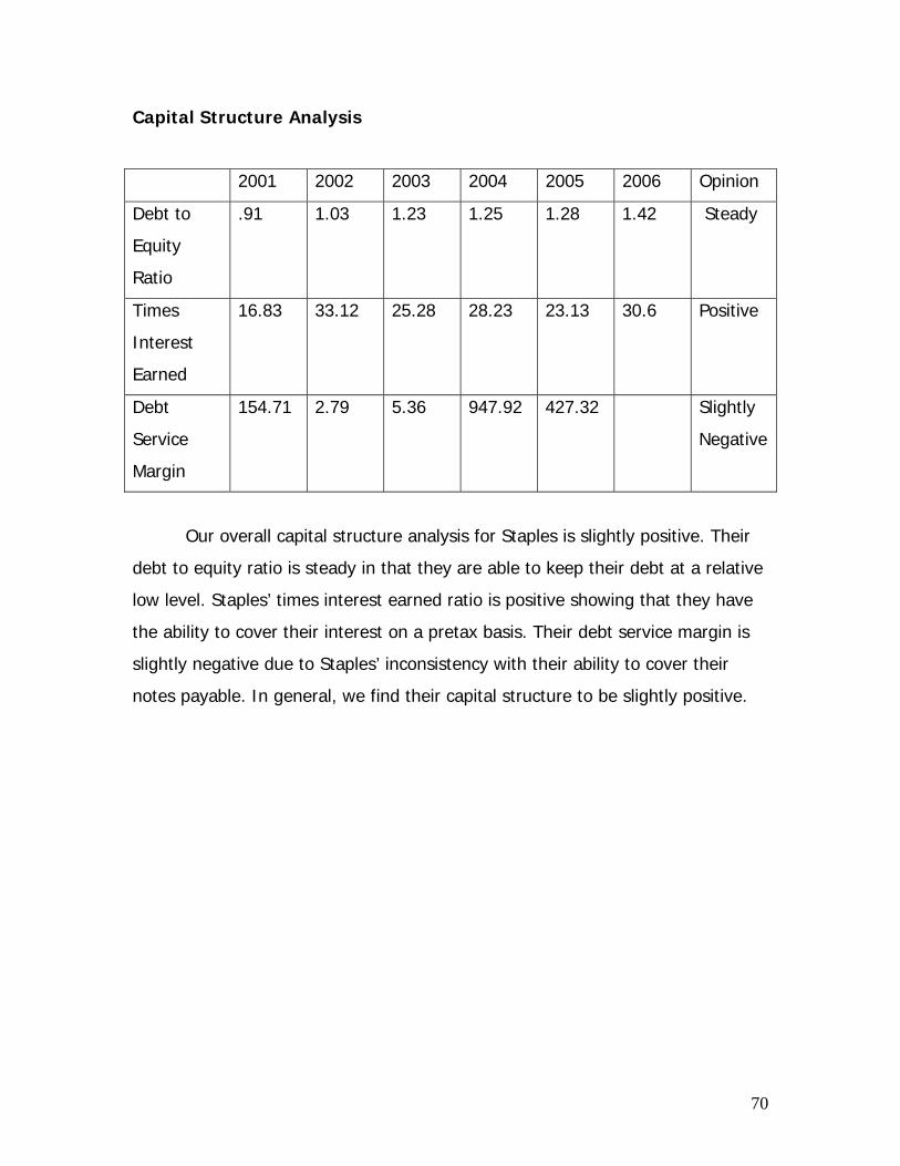
70
Capital Structure Analysis
Our overall capital structure analysis for Staples is slightly positive. Their
debt to equity ratio is steady in that they are able to keep their debt at a relative
low level. Staples’ times interest earned ratio is positive showing that they have
the ability to cover their interest on a pretax basis. Their debt service margin is
slightly negative due to Staples’ inconsistency with their ability to cover their
notes payable. In general, we find their capital structure to be slightly positive.
2001 2002 2003 2004 2005 2006 Opinion
Debt to
Equity
Ratio
.91 1.03 1.23 1.25 1.28 1.42 Steady
Times
Interest
Earned
16.83 33.12 25.28 28.23 23.13 30.6 Positive
Debt
Service
Margin
154.71 2.79 5.36 947.92 427.32 Slightly
Negative

71
Sustainable Growth Rate and Internal Growth Rate
SGR & IGR Ratios
Staples 2003 2004 2005 2006
SGR -4.24% 5.06% 8.07% 8.59%
IGR 28 22.5 28.7 32.4
Office Depot 2003 2004 2005 2006
SGR -0.01% -0.01% -0.01% -0.04%
IGR 0.06 0.05 0.04 0.08
OfficeMax 2003 2004 2005 2006
SGR 0.01% -0.01% 0.03% -0.01%
IGR -0.01 0.02 -0.02 0.01
The above table shows the sustainable growth rate for Staples and its
competitors over the past five years. The sustainable growth rate is a measure of
how Staples can grow without borrowing money. Staples has room to grow in
the future at about 8.6% with without having to make any changes to its
operating and financial policies. Staples does not start paying dividends until the
year 2005. Since they have only been paying dividends for two years it is not
possible to forecast a realistic growth rate for the future. The average SGR for
Staples is 4.37%. Staples management must have anticipated the growth of the
company around 2005 enabling them to start paying dividends. Staples SGR has
grown at a fairly reasonable pace while its competitors seem to be slowly
dwindling.
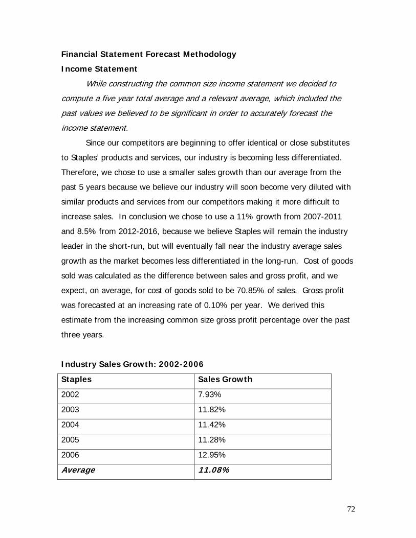
72
Financial Statement Forecast Methodology
Income Statement
While constructing the common size income statement we decided to
compute a five year total average and a relevant average, which included the
past values we believed to be significant in order to accurately forecast the
income statement.
Since our competitors are beginning to offer identical or close substitutes
to Staples’ products and services, our industry is becoming less differentiated.
Therefore, we chose to use a smaller sales growth than our average from the
past 5 years because we believe our industry will soon become very diluted with
similar products and services from our competitors making it more difficult to
increase sales. In conclusion we chose to use a 11% growth from 2007-2011
and 8.5% from 2012-2016, because we believe Staples will remain the industry
leader in the short-run, but will eventually fall near the industry average sales
growth as the market becomes less differentiated in the long-run. Cost of goods
sold was calculated as the difference between sales and gross profit, and we
expect, on average, for cost of goods sold to be 70.85% of sales. Gross profit
was forecasted at an increasing rate of 0.10% per year. We derived this
estimate from the increasing common size gross profit percentage over the past
three years.
Industry Sales Growth: 2002-2006
Staples Sales Growth
2002 7.93%
2003 11.82%
2004 11.42%
2005 11.28%
2006 12.95%
Average 11.08%

73
Office Depot
2002 2.48%
2003 8.82%
2004 9.76%
2005 5.27%
2006 5.13%
Average 6.29%
OfficeMax
2002 -0.13%
2003 11.23%
2004 60.95%
2005 -30.99%
2006 -2.10%
Average 7.79%
Industry Average 8.39%
Operating and selling expenses were forecasted using a decreasing rate of
0.05% per year. This rate was computed using the decreasing rate of operating
and selling expenses with respect to sales over the relevant past three years.
We believe our general and administrative expenses will remain near 4.25% of
sales, a slight increase from previous years. This increase is due to the costs we
believe will be associated with Staples entering new domestic and foreign
markets including the 110 new stores they plan to open in 2007. We avoided
increasing the amortization of intangibles from the most recent year at 0.08%.
This is due to a potential red flag observed earlier that rises from Staples’ failure
to recognize the impairment of goodwill and indefinite lived intangible assets
since the adoption of SFAS No. 142 on February 3, 2002. Since that date,
Staples has acquired numerous businesses worldwide. Total operating expenses
were calculated as the sum of operating and selling expenses, general and
74
administrative expenses, and the amortization of intangibles and operating
income was calculated as the difference between gross profit and total operating
expenses.
Interest income and interest expense were forecasted using constant
rates of 0.28% and 0.26% respectively using recent their recent trends.
Miscellaneous income (expense) was forecasted using the 5 year average of
0.01%. The sum of interest income, interest expense, and miscellaneous
interest (expense) equals interest and other expenses, which is added to
operating income to obtain income before taxes. Finally, forecasted net income
is derived using an increasing rate of 0.15% per year, which is smaller than the
average increase, because net income is increasing at a decreasing rate, and
income tax expense is calculated by the difference between income before taxes
and net income.

75
Staples Income Statements (in thousands)
Actual Financial Statements ASSUME ASSUME2002 2003 2004 2005 2006 2007 2008 2009 2010 2011 2012 2013 2014 2015 2016
2003/01/31 2004/01/28 2005/01/28 2006/01/28 2007/02/03
Sales $11596075 $12967022 $14448378 $16078852 $18160789 11% Growth/Year $20158476 $22375908 $24837258 $27569356 $30601986 8.5% Growth/Year $33203154 $36025423 $39087583 $42410028 $46014880
Cost of goods sold and occupancy costs $8652593 $9468890 $10343643 $11493310 $12966788 $14372976 $15931628 $17659269 $19574220 $21696782 $23507805 $25469943 $27595801 $29899034 $32394437
Gross profit $2943482 $3498132 $4104735 $4585542 $5194001 $5785500 $6444280 $7177989 $7995137 $8905204 $9695349 $10555479 $11491783 $12510994 $13620443
Operating and other expenses:
Operating and selling $1795428 $2167764 $2359551 $2617958 $2946249 $3260257 $3607697 $3992126 $4417475 $4888096 $5286983 $5718363 $6184880 $6689390 $7234981
Pre-opening $8746
General and administrative $454501 $524094 $610568 $641296 $770268 $856735 $950976 $1055583 $1171698 $1300584 $1411134 $1531080 $1661222 $1802426 $1955632
Amortization of intangibles $2135 $7986 $8743 $13008 $14415 $16127 $17901 $19870 $22055 $24482 $26563 $28820 $31270 $33928 $36812
Total operating expenses $2260810 $2699844 $2978862 $3272262 $3730932 $4133119 $4576574 $5067579 $5611228 $6213162 $6724679 $7278264 $7877373 $8525744 $9227425
Operating income $682672 $798288 $1125873 $1313280 $1463069 $1652380 $1867706 $2110410 $2383909 $2692042 $2970670 $3277215 $3614410 $3985250 $4393018
Other income (expense):
Interest income $10135 $31042 $59937 $58839 $56444 $62653 $69544 $77194 $85686 $92969 $100871 $109445 $118748 $128842
Interest expense -$31575 -$39888 -$56773 -$47810 -$52412 -$58177 -$64577 -$71680 -$79565 -$86328 -$93666 -$101628 -$110266 -$119639
Miscellaneous income (expense) $1264 -$1455 -$1945 -$2770 -$1955 -$2016 -$2119 -$2008 -$2412 -$2734 -$3056 -$3201 -$3428 -$3688
Interest and other expense, net -$20609 -$20176 -$10301 $1219 $8259 $2077 $2459 $2848 $3506 $3708 $3907 $4149 $4617 $5054 $5515
Income before income taxes and minority interest $662063 $778112 $1115572 $1314499 $1471328 $1656534 $1872624 $2116106 $2390920 $2699458 $2978484 $3285514 $3623643 $3995358 $4404049
Income tax expense $215963 $287901 $407184 $479792 $497972 $545515 $605828 $672708 $747394 $829240 $899493 $975771 $1058941 $1149041 $1246772
Income before minority interests $490211 $708388 $834707 $973356 .
Minority interest $ $ $298 -$321Net Income $446100 $490211 $708388 $834409 $973677 $1111019 $1266795 $1443399 $1643526 $1870217 $2078990 $2309743 $2564702 $2846317 $3157276
Forecasted Financial Statements

76
Common Size Income Statement - SPLSActual Financial Statements 5 Year Average Relevant Average ASSUME
2002 2003 2004 2005 2006 2007 2008 2009 2010 2011 2012 2013 2014 2015 20162003/01/31 2004/01/28 2005/01/28 2006/01/28 2007/02/03
Sales 100.00% 100.00% 100.00% 100.00% 100.00% 100.00% 100.00% 100.00% 100.00% 100.00% 100.00% 100.00% 100.00% 100.00% 100.00% 100.00% 100.00% 100.00%Cost of goods sold and occupancy costs 74.62% 73.02% 71.59% 71.48% 71.40% 72.42% 71.49% Calculated 71.30% 71.20% 71.10% 71.00% 70.90% 70.80% 70.70% 70.60% 70.50% 70.40%Gross profit 25.38% 26.98% 28.41% 28.52% 28.60% 27.58% 28.51% Increasing 0.10%/Year 28.70% 28.80% 28.90% 29.00% 29.10% 29.20% 29.30% 29.40% 29.50% 29.60%Operating and other expenses:Operating and selling 15.48% 16.72% 16.33% 16.28% 16.22% 16.21% 16.28% Decreasing 0.05%/Year 16.17% 16.12% 16.07% 16.02% 15.97% 15.92% 15.87% 15.82% 15.77% 15.72%Pre-opening 0.08% 0.00% 0.00% 0.00% 0.00% 0.02%General and administrative 3.92% 4.04% 4.23% 3.99% 4.24% 4.08% 4.08% 4.25% 4.25% 4.25% 4.25% 4.25% 4.25% 4.25% 4.25% 4.25% 4.25% 4.25%Amortization of intangibles 0.02% 0.06% 0.06% 0.08% 0.08% 0.06% 0.06% 0.08% 0.08% 0.08% 0.08% 0.08% 0.08% 0.08% 0.08% 0.08% 0.08% 0.08%Total operating expenses 19.50% 20.82% 20.62% 20.35% 20.54% 20.37% 20.58% Calculated 20.50% 20.45% 20.40% 20.35% 20.30% 20.25% 20.20% 20.15% 20.10% 20.05%Operating income 5.89% 6.16% 7.79% 8.17% 8.06% 7.21% 8.01% Calculated 8.20% 8.35% 8.50% 8.65% 8.80% 8.95% 9.10% 9.25% 9.40% 9.55%Other income (expense):Interest income 0.00% 0.08% 0.21% 0.37% 0.32% 0.20% 0.30% 0.28% 0.28% 0.28% 0.28% 0.28% 0.28% 0.28% 0.28% 0.28% 0.28% 0.28%Interest expense 0.00% -0.24% -0.28% -0.35% -0.26% -0.23% -0.28% -0.26% -0.26% -0.26% -0.26% -0.26% -0.26% -0.26% -0.26% -0.26% -0.26% -0.26%Miscellaneous income (expense) 0.00% 0.01% -0.01% -0.01% -0.02% -0.01% -0.01% -0.01% -0.01% -0.01% -0.01% -0.01% -0.01% -0.01% -0.01% -0.01% -0.01% -0.01%Interest and other expense, net -0.18% -0.16% -0.07% 0.01% 0.05% -0.03% 0.01% Calculated 0.01% 0.01% 0.01% 0.01% 0.01% 0.01% 0.01% 0.01% 0.01% 0.01%Income before income taxes and minority interest 5.71% 6.00% 7.72% 8.18% 8.10% 7.14% 8.03% Calculated 8.22% 8.37% 8.52% 8.67% 8.82% 8.97% 9.12% 9.27% 9.42% 9.57%Income tax expense 1.86% 2.22% 2.82% 2.98% 2.74% 2.53% 2.85% Calculated 2.71% 2.71% 2.71% 2.71% 2.71% 2.71% 2.71% 2.71% 2.71% 2.71%Income before minority interests 0.00% 3.78% 4.90% 5.19% 5.36% 3.85% Minority interest 0.00% 0.00% 0.00% 0.00% 0.00% 0.00%Net Income 3.85% 3.78% 4.90% 5.19% 5.36% 4.62% 5.15% Increasing 0.15%/Year 5.51% 5.66% 5.81% 5.96% 6.11% 6.26% 6.41% 6.56% 6.71% 6.86%
Forecasted Financial Statements
77
Balance Sheet
To forecast the balance sheet of Staples, we began by taking an average
of the percentage of total assets to sales in each of the previous five years. In
doing so, we found that total assets are, on average, 48.5% of sales. We
ultimately decided to use 45% because in recent years, Staples’ sales have
increased greater compared to its total assets. We then multiplied this
percentage with each year’s forecasted sales values to arrive at a forecasted
value for total assets.
Once we had forecasted values for the firm’s total assets we could begin
to forecast all the assets of the firm. In most cases, we took an average
percentage of total assets for the previous five years to arrive at our forecasted
asset values. While this proved to work with many of the asset categories, in
some cases, the average was not an accurate forecast index to use. For
example, on average, accounts receivable were 7.32% of total assets in the
previous five years. However, we used 9% given the recent three year upward
trend of the receivables to total assets percentage.
The ten year forecasts of Staples’ liabilities and stockholder’s equity were
obtained using the same technique. We found an average percentage of each
line item to total assets. We found current liabilities to be 32% of total assets
and total liabilities to be 42% of total assets, both averaged over the previous
five years. We found stockholder’s equity to be an average of 58% of total
assets over the previous five years.

78
Balance Sheets - SPLS (in thousands)ASSUME
2002 2003 2004 2005 2006 2007 2008 2009 2010 2011 2012 2013 2014 2015 20162003/01/31 2004/01/28 2005/01/28 2006/01/28 2007/02/03
AssetsCurrent assets: Cash and cash equivalents $596064 $457465 $997310 $977822 $1017671 $1088558 $1208299 $1341212 $1488745 $1652507 $1792970 $1945373 $2110730 $2290142 $2484804 Short-term investments $100175 $934275 $472231 $593082 $457759 $598707 $664564 $737667 $818810 $908879 $986134 $1069955 $1160901 $1259578 $1366642 Receivables, net $364419 $410330 $485126 $576672 $720797 $816418 $906224 $1005909 $1116559 $1239380 $1344728 $1459030 $1583047 $1717606 $1863603 Merchandise inventories, net $1555205 $1465989 $1602530 $1706372 $1919714 $2120373 $2265561 $2514772 $2791397 $3098451 $3361819 $3647574 $3957618 $4294015 $4659007 Deferred income tax asset $96229 $96247 $86041 $149257 $141108 Prepaid expenses and other current assets $105559 $114598 $138374 $141339 $174314 Total current assets $2717476 $3478904 $3781612 $4144544 $4431363 $4807796 $5336654 $5923686 $6575292 $7298574 $7918952 $8592063 $9322389 $10114792 $10974549Property and equipment: Land and buildings $524730 $601063 $649175 $705978 $791264 $907131 $1006916 $1117677 $1240621 $1377089 $1494142 $1621144 $1758941 $1908451 $2070670 Leasehold improvements $621713 $692837 $762946 $884853 $996434 $1088558 $1208299 $1341212 $1488745 $1652507 $1792970 $1945373 $2110730 $2290142 $2484804 Equipment $951439 $1045605 $1140234 $1330181 $1539617 $1700871 $1887967 $2095644 $2326164 $2582043 $2801516 $3039645 $3298015 $3578346 $3882506 Furniture and fixtures $472935 $533104 $597293 $672931 $757408 $816418 $906224 $1005909 $1116559 $1239380 $1344728 $1459030 $1583047 $1717606 $1863603 Total property and equipment $2570817 $2872609 $3149648 $3593943 $4084723 $4399587 $4883542 $5420732 $6017012 $6678883 $7246588 $7862548 $8530865 $9255989 $10042748 Less accumulated depreciation and amortization $1123065 $1367308 $1548774 $1835549 $2110602 -$2358542 -$2617981 -$2905959 -$3225615 -$3580432 -$3884769 -$4214974 -$4573247 -$4961973 -$5383741 Net property and equipment $1447752 $1505301 $1600874 $1758394 $1974121 $2177115 $2416598 $2682424 $2977490 $3305014 $3585941 $3890746 $4221459 $4580283 $4969607Lease acquisition costs, net of accumulated amortization $51450 $44227 $38400 $34885 $33579 $27214 $30207 $33530 $37219 $41313 $44824 $48634 $52768 $57254 $62120Intangible assets, net of accumulated amortization $216391 $209541 $222520 $240395 $232383Goodwill $1207824 $1202007 $1321464 $1378752 $1455113defferred income taxesOther assets $80495 $63066 $106578 $119619 $270706 Total assets $5721388 $6503046 $7071448 $7676589 $8397265 45% of sales $9071314 $10069159 $11176766 $12406210 $13770894 $14941419 $16211440 $17589413 $19084513 $20706696
LiabilitiesCurrent liabilities: Accounts payable $1092172 $1110631 $1241433 $1435815 $1486188 $1610158 $1787276 $1983876 $2202102 $2444334 $2652102 $2877531 $3122121 $3387501 $3675439
Accrued expenses and other current liabilities $755483 $822453 $954184 $1041200 $1101018 $1197413 $1329129 $1475333 $1637620 $1817758 $1972267 $2139910 $2321802 $2519156 $2733284 Debt maturing within one year $327671 $190150 $1244 $2891 $201177 Total current liabilities $2175326 $2123234 $2196861 $2479906 $2788383 32% of TA $2902821 $3222131 $3576565 $3969987 $4406686 $4781254 $5187661 $5628612 $6107044 $6626143Long-term debt $732041 $567433 $557927 $527606 $316465 $453566 $503458 $558838 $620311 $688545 $747071 $810572 $879471 $954226 $1035335Deferred income tax liability $50267 $7563 $23314 $5845 $8986Other long-term obligations $104862 $141916 $178150 $233426 $252657 $244925 $271867 $301773 $334968 $371814 $403418 $437709 $474914 $515282 $559081Minority interest $4335 $9109 Total liabilities $3062496 $2840146 $2956252 $3251118 $3375600 42% of TA $3809952 $4229047 $4694242 $5210608 $5783775 $6275396 $6808805 $7387553 $8015495 $8696812Adjusted total Liabilities $3151758 $3101264 $2989391 $2804825 $2534544 $3946205 $3384399 $2705971 $1896045 $938079
Stockholders Equity:Common stock $299 $316 $488 $498 $510Additional paid-in capital $1484833 $1933379 $2254947 $2544692 $3338412Cumulative foreign currency translation adjustments $11481 $81002 $114427 $87085 $189115Retained earnings $1719091 $2209302 $2818163 $3529170 $4005424 $4172804 $4631813 $5141312 $5706857 $6334611 $6873053 $7457262 $8091130 $8778876 $9525080Less: treasury stock -$556812 -$561099 -$1072829 -$1735974 -$2511796 Total stockholders equity $2658892 $3662900 $4115196 $4425471 $5021665 $5261362 $5840112 $6482524 $7195602 $7987118 $8666023 $9402635 $10201859 $11069017 $12009884Adjusted total Retained Earnings $4903315 $5951654 $7171134 $8585145 $10220108 $9978973 $11810800 $13867201 $16172227 $18752376Adjusted total equity $5919556 $6967895 $8187375 $9601386 $11236349 $10995214 $12827041 $14883442 $17188468 $19768617
Total liabilities and stockholders equity $5721388 $6503046 $7071448 $7676589 $8397265 $9071314 $10069159 $11176766 $12406210 $13770894 $14941419 $16211440 $17589413 $19084513 $20706696
Total Assets $9071314 $10069159 $11176766 $12406210 $13770894 $14941419 $16211440 $17589413 $19084513 $20706696Forecasted DPS $0.30 $0.30 $0.31 $0.32 $0.33 $0.34 $0.34 $0.35 $0.36 $0.37Forecasted Total Dividends 717 $213128 $218456 $223918 $229516 $235254 $241135 $247163 $253343 $259676 $266168∆ Adjusted Total Equity 17.71% 17.50% 17.27% 17.03% -2.15% 16.66% 16.03% 15.49% 15.01% N/A
Forecasted Financial StatementsActual Financial Statements

79
Common Size Balance Sheet - SPLSActual Financial Statements AVG ASSUME
2002 2003 2004 2005 2006 2007 2008 2009 2010 2011 2012 2013 2014 2015 20162003/02/01 2004/01/31 2005/01/28 2006/01/28 2007/02/03
AssetsCurrent assets: Cash and cash equivalents 10.42% 7.03% 14.10% 12.74% 12.12% 12% 12.00% 12.00% 12.00% 12.00% 12.00% 12.00% 12.00% 12.00% 12.00% 12.00% Short-term investments 1.75% 14.37% 6.68% 7.73% 5.45% 6.62% 6.60% 6.60% 6.60% 6.60% 6.60% 6.60% 6.60% 6.60% 6.60% 6.60% 6.60% Receivables, net 6.37% 6.31% 6.86% 7.51% 8.58% 7.32% 9% 9.00% 9.00% 9.00% 9.00% 9.00% 9.00% 9.00% 9.00% 9.00% 9.00% Merchandise inventories, net 27.18% 22.54% 22.66% 22.23% 22.86% 22.57% 22.50% 22.50% 22.50% 22.50% 22.50% 22.50% 22.50% 22.50% 22.50% 22.50% 22.50% Deferred income tax asset 1.68% 1.48% 1.22% 1.94% 1.68% Prepaid expenses and other current assets 1.84% 1.76% 1.96% 1.84% 2.08% Total current assets 47.50% 53.50% 53.48% 53.99% 52.77% 53.43% 53% 53.00% 53.00% 53.00% 53.00% 53.00% 53.00% 53.00% 53.00% 53.00% 53.00%Property and equipment: Land and buildings 9.17% 9.24% 9.18% 9.20% 9.42% 10% 10.00% 10.00% 10.00% 10.00% 10.00% 10.00% 10.00% 10.00% 10.00% 10.00% Leasehold improvements 10.87% 10.65% 10.79% 11.53% 11.87% 12% 12.00% 12.00% 12.00% 12.00% 12.00% 12.00% 12.00% 12.00% 12.00% 12.00% Equipment 16.63% 16.08% 16.12% 17.33% 18.33% 18.75% 18.75% 18.75% 18.75% 18.75% 18.75% 18.75% 18.75% 18.75% 18.75% 18.75% Furniture and fixtures 8.27% 8.20% 8.45% 8.77% 9.02% 9% 9.00% 9.00% 9.00% 9.00% 9.00% 9.00% 9.00% 9.00% 9.00% 9.00% Total property and equipment 44.93% 44.17% 44.54% 46.82% 48.64% 46.67% 48.50% 48.50% 48.50% 48.50% 48.50% 48.50% 48.50% 48.50% 48.50% 48.50% 48.50% Less accumulated depreciation and amortization 19.63% 21.03% 21.90% 23.91% 25.13% 26% -26.00% -26.00% -26.00% -26.00% -26.00% -26.00% -26.00% -26.00% -26.00% -26.00% Net property and equipment 25.30% 23.15% 22.64% 22.91% 23.51% 24% 24.00% 24.00% 24.00% 24.00% 24.00% 24.00% 24.00% 24.00% 24.00% 24.00%Lease acquisition costs, net of accumulated amortization 0.90% 0.68% 0.54% 0.45% 0.40% 0.30% 0.30% 0.30% 0.30% 0.30% 0.30% 0.30% 0.30% 0.30% 0.30% 0.30%
Intangible assets, net of accumulated amortization 3.78% 3.22% 3.15% 3.13% 2.77%Goodwill 21.11% 18.48% 18.69% 17.96% 17.33%defferred income taxes 0.00% 0.00% 0.00% 0.00% 0.00%Other assets 1.41% 0.97% 1.51% 1.56% 3.22% Total assets 100.00% 100.00% 100.00% 100.00% 100.00% 100.00% 100.00% 100.00% 100.00% 100.00% 100.00% 100.00% 100.00% 100.00% 100.00%
LiabilitiesCurrent liabilities: Accounts payable 19.09% 17.08% 17.56% 18.70% 17.70% 17.76% 17.75% 17.75% 17.75% 17.75% 17.75% 17.75% 17.75% 17.75% 17.75% 17.75% 17.75%
Accrued expenses and other current liabilities 13.20% 12.65% 13.49% 13.56% 13.11% 13.20% 13.20% 13.20% 13.20% 13.20% 13.20% 13.20% 13.20% 13.20% 13.20% 13.20% 13.20% Debt maturing within one year 5.73% 2.92% 0.02% 0.04% 2.40% Total current liabilities 38.02% 32.65% 31.07% 32.30% 33.21% 32% of TA 32.00% 32.00% 32.00% 32.00% 32.00% 32.00% 32.00% 32.00% 32.00% 32.00%Long-term debt 12.79% 8.73% 7.89% 6.87% 3.77% 8.01% 5% 5.00% 5.00% 5.00% 5.00% 5.00% 5.00% 5.00% 5.00% 5.00% 5.00%Deferred income tax liability 0.88% 0.12% 0.33% 0.08% 0.11%Other long-term obligations 1.83% 2.18% 2.52% 3.04% 3.01% 2.69% 2.70% 2.70% 2.70% 2.70% 2.70% 2.70% 2.70% 2.70% 2.70% 2.70% 2.70%Minority interest 0.00% 0.00% 0.00% 0.06% 0.11% Total liabilities 53.53% 43.67% 41.81% 42.35% 40.20% 42.01% 42% of TA 42.00% 42.00% 42.00% 42.00% 42.00% 42.00% 42.00% 42.00% 42.00% 42.00%
Stockholders Equity:Common stock 0.01% 0.00% 0.01% 0.01% 0.01% 0.01% 0.01% 0.01% 0.01% 0.01% 0.01% 0.01% 0.01% 0.01% 0.01% 0.01%Additional paid-in capital 25.95% 29.73% 31.89% 33.15% 39.76% 33.63% 35% 35.00% 35.00% 35.00% 35.00% 35.00% 35.00% 35.00% 35.00% 35.00% 35.00%Cumulative foreign currency translation adjustments 0.20% 1.25% 1.62% 1.13% 2.25%Retained earnings 30.05% 33.97% 39.85% 45.97% 47.70% 44.51% 46% 46.00% 46.00% 46.00% 46.00% 46.00% 46.00% 46.00% 46.00% 46.00% 46.00%Less: treasury stock -9.73% -8.63% -15.17% -22.61% -29.91% Total stockholders equity 46.47% 56.33% 58.19% 57.65% 59.80% 57.99% 58% 58.00% 58.00% 58.00% 58.00% 58.00% 58.00% 58.00% 58.00% 58.00% 58.00%
Total Liabilities and Stockholders Equity 100.00% 100.00% 100.00% 100.00% 100.00% 100.00% 100.00% 100.00% 100.00% 100.00% 100.00% 100.00% 100.00% 100.00% 100.00% 100.00%
Forecasted Financial Statements
80
Cash Flows Statement
When forecasting the statement of cash flows, we first created a common
size cash flow statement to get an idea of the percentage of cash flows from
operations. This helped us analyze each line item to determine whether or not
there was a growth pattern present. If a pattern is in fact present, then the line
item is further analyzed and the first steps of forecasting begin. For the
forecasting of net income we used the same growth percentages as net sales;
for years 2006 – 2011 the growth rate is 11% and for 2012 – 2016 the growth
rate is 8.5%. To better explain, the net income for 2005 is 973,677,000, taking
this number and multiplying it by 11% gives you the forecasted net income for
2006: 1,080,781,470. The same method used for net income was also used for
depreciation and amortization. A different method was used in the forecasting of
net cash provided by operating activities. This forecast was computed by
obtaining the growth percentage from years 2002 to 2004 and taking the
average of these three percentages. This average is then continuously multiplied
each year by the previous year’s cash from operating activities, ultimately giving
you the forecasted cash from operating activities. In addition, we also took the
average over the past five years of many line items to assist us in the forecasting
of the cash flows statement. Lastly, we were unable to forecast many items due
to the fact that there were no apparent trends in the numbers.
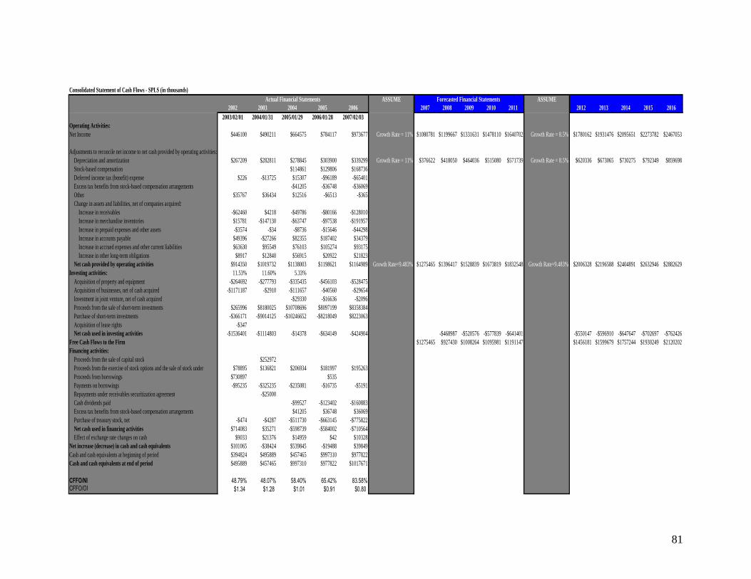
81
ASSUME Forecasted Financial Statements ASSUME2002 2003 2004 2005 2006 2007 2008 2009 2010 2011 2012 2013 2014 2015 2016
2003/02/01 2004/01/31 2005/01/29 2006/01/28 2007/02/03Operating Activities:Net Income $446100 $490211 $664575 $784117 $973677 Growth Rate = 11% $1080781 $1199667 $1331631 $1478110 $1640702 Growth Rate = 8.5% $1780162 $1931476 $2095651 $2273782 $2467053
Adjustments to reconcile net income to net cash provided by operating activities: Depreciation and amortization $267209 $282811 $278845 $303900 $339299 Growth Rate = 11% $376622 $418050 $464036 $515080 $571739 Growth Rate = 8.5% $620336 $673065 $730275 $792349 $859698 Stock-based compensation $114861 $129806 $168736 Deferred income tax (benefit) expense $226 -$13725 $15307 -$96189 -$65401 Excess tax benefits from stock-based compensation arrangements -$41205 -$36748 -$36069 Other $35767 $36434 $12516 -$6513 -$365 Change in assets and liabilities, net of companies acquired: Increase in receivables -$62460 $4218 -$49786 -$80166 -$128010 Increase in merchandise inventories $15781 -$147130 -$63747 -$97538 -$191957 Increase in prepaid expenses and other assets -$3574 -$34 -$8736 -$15646 -$44298 Increase in accounts payable $49396 -$27266 $82355 $187402 $34379 Increase in accrued expenses and other current liabilities $63630 $95549 $76103 $105274 $93175 Increase in other long-term obligations $8917 $12840 $56915 $20922 $21823 Net cash provided by operating activities $914350 $1019732 $1138003 $1198621 $1164989 Growth Rate=9.483% $1275465 $1396417 $1528839 $1673819 $1832548 Growth Rate=9.483% $2006328 $2196588 $2404891 $2632946 $2882629Investing activities: 11.53% 11.60% 5.33% Acquisition of property and equipment -$264692 -$277793 -$335435 -$456103 -$528475 Acquisition of businesses, net of cash acquired -$1171187 -$2910 -$111657 -$40560 -$29654 Investment in joint venture, net of cash acquired -$29330 -$16636 -$2096 Proceeds from the sale of short-term investments $265996 $8180025 $10708696 $8097199 $8358384 Purchase of short-term investments -$366171 -$9014125 -$10246652 -$8218049 $8223063 Acquisition of lease rights -$347 Net cash used in investing activities -$1536401 -$1114803 -$14378 -$634149 -$424904 -$468987 -$520576 -$577839 -$641401 -$550147 -$596910 -$647647 -$702697 -$762426Free Cash Flows to the Firm $1275465 $927430 $1008264 $1095981 $1191147 $1456181 $1599679 $1757244 $1930249 $2120202Financing activities: Proceeds from the sale of capital stock $252972 Proceeds from the exercise of stock options and the sale of stock under $78895 $136821 $206934 $181997 $195263 Proceeds from borrowings $730897 $535 Payments on borrowings -$95235 -$325235 -$235081 -$16735 -$5191 Repayments under receivables securitization agreement -$25000 Cash dividends paid -$99527 -$123402 -$160883 Excess tax benefits from stock-based compensation arrangements $41205 $36748 $36069 Purchase of treasury stock, net -$474 -$4287 -$511730 -$663145 -$775822 Net cash used in financing activities $714083 $35271 -$598739 -$584002 -$710564 Effect of exchange rate changes on cash $9033 $21376 $14959 $42 $10328Net increase (decrease) in cash and cash equivalents $101065 -$38424 $539845 -$19488 $39849Cash and cash equivalents at beginning of period $394824 $495889 $457465 $997310 $977822Cash and cash equivalents at end of period $495889 $457465 $997310 $977822 $1017671
CFFO/NI 48.79% 48.07% 58.40% 65.42% 83.58%CFFO/OI $1.34 $1.28 $1.01 $0.91 $0.80
Consolidated Statement of Cash Flows - SPLS (in thousands)Actual Financial Statements
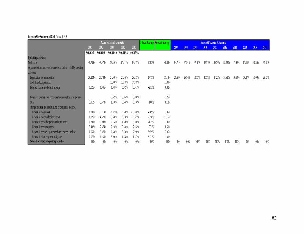
82
Common Size Statement of Cash Flows - SPLSActual FinancialStatements 5 Year Average Relevant Average Forecast Financial Statements
2002 2003 2004 2005 2006 2007 2008 2009 2010 2011 2012 2013 2014 2015 20162003/02/01 2004/01/31 2005/01/29 2006/01/28 2007/02/03
Operating Activities:Net Income 48.789% 48.073% 58.398% 65.418% 83.578% 60.85% 60.85% 84.74% 85.91% 87.10% 88.31% 89.53% 88.73% 87.93% 87.14% 86.36% 85.58%Adjustments to reconcile net income to net cash provided by operating activities: Depreciation and amortization 29.224% 27.734% 24.503% 25.354% 29.125% 27.19% 27.19% 29.53% 29.94% 30.35% 30.77% 31.20% 30.92% 30.64% 30.37% 30.09% 29.82% Stock-based compensation 10.093% 10.830% 14.484% 11.80% Deferred income tax (benefit) expense 0.025% -1.346% 1.345% -8.025% -5.614% -2.72% -6.82%
Excess tax benefits from stock-based compensation arrangements -3.621% -3.066% -3.096% -3.26% Other 3.912% 3.573% 1.100% -0.543% -0.031% 1.60% 0.18% Change in assets and liabilities, net of companies acquired: Increase in receivables -6.831% 0.414% -4.375% -6.688% -10.988% -5.69% -7.35% Increase in merchandise inventories 1.726% -14.428% -5.602% -8.138% -16.477% -8.58% -11.16% Increase in prepaid expenses and other assets -0.391% -0.003% -0.768% -1.305% -3.802% -1.25% -1.96% Increase in accounts payable 5.402% -2.674% 7.237% 15.635% 2.951% 5.71% 8.61% Increase in accrued expenses and other current liabilities 6.959% 9.370% 6.687% 8.783% 7.998% 7.959% 7.96% Increase in other long-term obligations 0.975% 1.259% 5.001% 1.746% 1.873% 2.171% 1.81% Net cash provided by operating activities 100% 100% 100% 100% 100% 100% 100% 100% 100% 100% 100% 100% 100% 100% 100% 100% 100%

83
Analysis of Valuations
Cost of Capital
The cost of capital is an important factor for analysts to consider because
it is “the overall required return on the firm as a whole and, as such, it is often
used internally by company directors to determine the economic feasibility of
expansionary opportunities and mergers. It is the appropriate discount rate to
use for cash flows with risk that is similar to that of the overall firm”
(investopedia.com). It is computed as a weighted average of the value of debt
and equity to the firm.
Cost of Equity
To estimate the cost of equity, we use the CAPM model. To do
this, we first had to obtain market prices for Staples, S&P 500 monthly returns,
and government risk-free rates. We used the 10 year, 7 year, 5 year, 1 year,
and 3 month treasury bill rates. We obtained a market risk premium for each
treasury rate by subtracting it from the market, or S&P 500, returns. From
there, we ran a regression for 2, 3, 4, 5, and 6 years. From the regression
results, we were able to obtain a beta of 1.15. We concluded this because the
R^2 value, 23.15%, was the largest of all the regression models. With the
attainment of a beta value, we could now estimate the cost of equity using the
CAPM model. The cost of equity is important because it is the required rate of
return for investors. In other words, it is the minimum rate of return that will
induce an investor to buy. Our CAPM model is:
Ke = 0.0313 + 1.15(.0617)

84
Beta R^2 KE Beta R^2 KE24 month 0.35528 -0.03938 0.06347 24 month 0.36017 -0.03922 0.0624836 month 0.68603 0.00395 0.07862 36 month 0.68862 0.00414 0.0781548 month 0.62676 0.01572 0.07591 48 month 0.62677 0.01583 0.0752060 month 1.16314 0.20306 0.10047 60 month 1.16301 0.20311 0.1007872 month 1.14619 0.22953 0.09970 72 month 1.14573 0.22949 0.09995
RF = 0.0472 RF = 0.0453
Beta R^2 KE Beta R^2 KE24 month 0.36502 -0.03905 0.06100 24 month 0.39384 -0.03806 0.0569936 month 0.69114 0.00431 0.07743 36 month 0.70952 0.00578 0.0757548 month 0.62677 0.01597 0.07419 48 month 0.63336 0.01715 0.0712260 month 1.16327 0.20316 0.10123 60 month 1.16773 0.20414 0.1029672 month 1.14607 0.22962 0.10036 72 month 1.15041 0.23094 0.10193
RF = 0.0426 RF = 0.0336
Beta R^2 KE24 month 0.40605 -0.03762 0.0563536 month 0.71746 0.00649 0.0755748 month 0.63857 0.01770 0.0707060 month 1.17050 0.20492 0.1035272 month 1.15183 0.23153 0.10237
RF = 0.0313
GS 3 MONTH Summary
GS10 Summary GS7 Summary
GS5 Summary GS1 Summary
We obtained the risk-free rate by taking an average of the yearly returns
for each risk-free rate series. We ultimately used the 3 month average risk-free
return because it correlated with the highest R^2 value. In addition, we
concluded the market return was 0.093. We obtained this value by taking an
average of the S&P 500 monthly returns. The market risk premium, 0.0617, was
calculated by subtracting the risk-free rate from the average S&P 500 monthly
returns (0.093 – 0.0313). Solving the CAPM equation, we were able to calculate
a cost of equity of 10.237%.

85
Cost of Debt
The cost of debt is calculated using current and long-term liabilities from
the balance sheet. The different interest rates associated with the debt were
found directly in Staples’ 10-K, on the St. Louis Federal Reserve website, or were
reasonably estimated using available data for Staples, Office Depot, and
OfficeMax. The interest rates for accounts payable and accrued expenses and
liabilities are set equal to the one month commercial paper rate of 5.24%. The
interest rate for debt maturing within one year is given in Staples’ 10-K as
4.25%. The estimated interest rate for long-term liabilities was calculated using
an average of all available interest rates for long-term liabilities found in Staples’
10-K. The interest rate for long-term debt was directly stated in the 10-K at a
rate of 7.33%, and the deferred income tax liabilities are set equal to the risk
free rate of a one month treasury bill found on the St. Louis Federal Reserve’s
website. The line items contained within current and long-term liabilities on the
balance sheet are weighted using total liabilities. The sum of each line item’s
interest rate multiplied by its weight equals the total cost of debt of 5.547%.
Weighted Average Cost of Capital
To compute the after tax weighted average cost of capital we use the
value of debt, value of equity, cost of debt, cost of equity, and the tax rate. To
compute WACC, we used the following formula:
WACC = [Vd/(Vd+Ve)]rd(1-T) + [Ve/(Vd+Ve)]re
To find the market value of the equity we simply found the difference
between the market capitalization, the total value of the company, and the value
of the debt. This is represented by the following formula:
VF=VD+VE
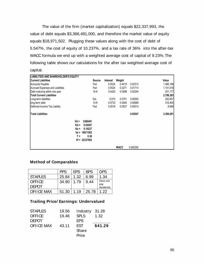
86
The value of the firm (market capitalization) equals $22,337,993, the
value of debt equals $3,366,491,000, and therefore the market value of equity
equals $18,971,502. Plugging these values along with the cost of debt of
5.547%, the cost of equity of 10.237%, and a tax rate of 36% into the after-tax
WACC formula we end up with a weighted average cost of capital of 9.23%.The
following table shows our calculations for the after tax weighted average cost of
capital.
LIABILITIES AND SHAREHOLDER'S EQUITYCurrent Liabilities Source Interest Weight ValueAccounts Payable Fed 0.0524 0.4415 0.02313 1,486,188Accrued Expenses and Liabilities Fed 0.0524 0.3271 0.01714 1,101,018Debt maturing within one year 10-K 0.0425 0.0598 0.00254 201,177Total Current Liabilities 2,788,383Long-term liabilities Est. 0.075 0.0751 0.00563 252,657long-term debt 10-K 0.0733 0.0940 0.00689 316,465Deferred Income Tax Liability Fed 0.0518 0.0027 0.00014 8,986
Total Liabilities 0.05547 3,366,491
Vd = 3366491Kd = 0.05547Ke = 0.10237Ve = 18971502
T = 0.36Vf = 22337993
WACC 0.092292
Method of Comparables PPS EPS BPS DPS STAPLES 25.84 1.32 6.99 1.34 OFFICE DEPOT
34.90 1.79 9.44 Does not pay dividends
OFIICE MAX 51.30 1.19 25.78 1.22 Trailing Price/Earnings: Undervalued STAPLES 19.56 Industry 31.28 OFFICE DEPOT
19.46 SPLS EPS
1.32
OFIICE MAX 43.11 EST Share Price
$41.29
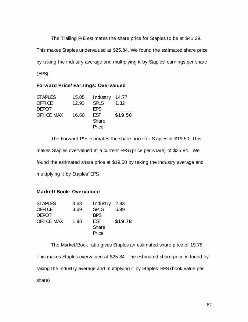
87
The Trailing P/E estimates the share price for Staples to be at $41.29.
This makes Staples undervalued at $25.84. We found the estimated share price
by taking the industry average and multiplying it by Staples’ earnings per share
(EPS).
Forward Price/Earnings: Overvalued STAPLES 15.05 Industry 14.77 OFFICE DEPOT
12.93 SPLS EPS
1.32
OFIICE MAX 16.60 EST Share Price
$19.50
The Forward P/E estimates the share price for Staples at $19.50. This
makes Staples overvalued at a current PPS (price per share) of $25.84. We
found the estimated share price at $19.50 by taking the industry average and
multiplying it by Staples’ EPS.
Market/Book: Overvalued STAPLES 3.68 Industry 2.83 OFFICE DEPOT
3.69 SPLS BPS
6.99
OFIICE MAX 1.98 EST Share Price
$19.78
The Market/Book ratio gives Staples an estimated share price of 19.78.
This makes Staples overvalued at $25.84. The estimated share price is found by
taking the industry average and multiplying it by Staples’ BPS (book value per
share).
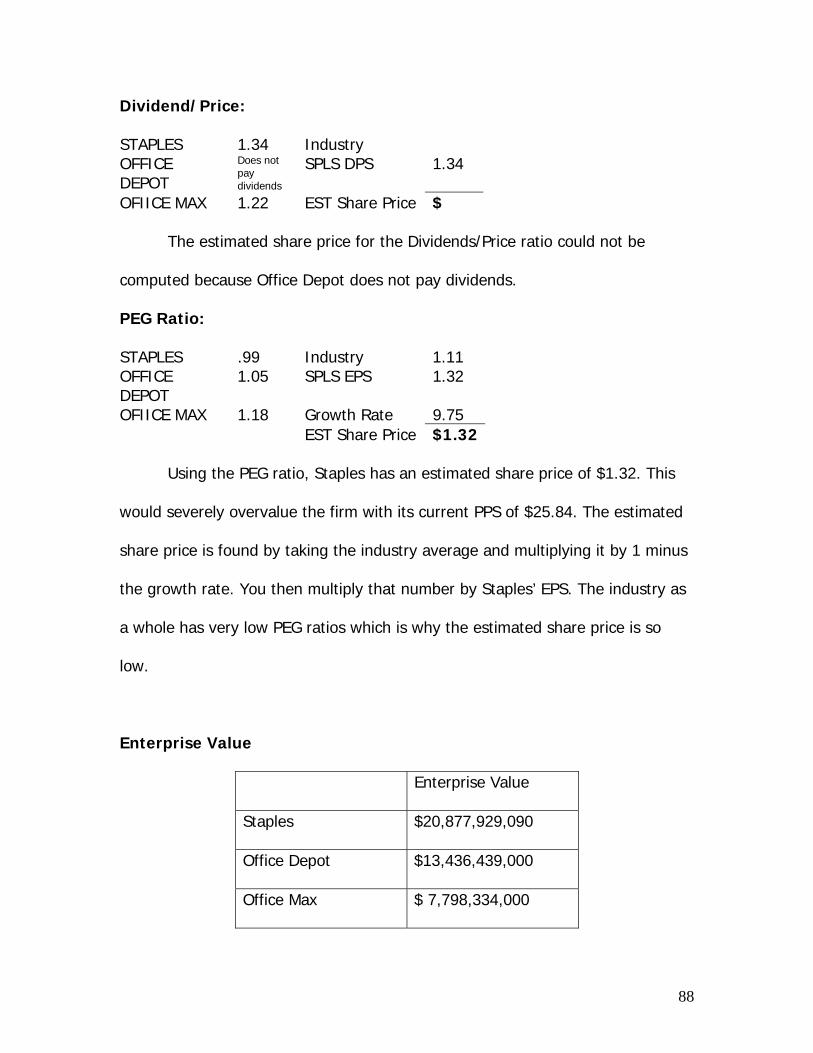
88
Dividend/Price: STAPLES 1.34 Industry OFFICE DEPOT
Does not pay dividends
SPLS DPS 1.34
OFIICE MAX 1.22 EST Share Price $ The estimated share price for the Dividends/Price ratio could not be
computed because Office Depot does not pay dividends.
PEG Ratio: STAPLES .99 Industry 1.11 OFFICE DEPOT
1.05 SPLS EPS 1.32
OFIICE MAX 1.18 Growth Rate 9.75 EST Share Price $1.32 Using the PEG ratio, Staples has an estimated share price of $1.32. This
would severely overvalue the firm with its current PPS of $25.84. The estimated
share price is found by taking the industry average and multiplying it by 1 minus
the growth rate. You then multiply that number by Staples’ EPS. The industry as
a whole has very low PEG ratios which is why the estimated share price is so
low.
Enterprise Value
Enterprise Value
Staples $20,877,929,090
Office Depot $13,436,439,000
Office Max $ 7,798,334,000

89
The enterprise value tells us the theoretical takeover price. It is computed
by adding together the market value of equity and the book value of liabilities
and then subtracting cash and cash equivalents. Currently, Staples leads the
industry with the highest buy out price. Staples has the most stable buyout price
too because of their increasing assets and low levels of debt.
Intrinsic Valuation Models
Given our previous forecasts and estimates we can derive an intrinsic
value using different valuation models. These models include the discount
dividends, discounted free cash flows, residual income, abnormal earnings
growth, and long run return on equity models. It is known that the residual
income model has the largest explanatory power, while the discount dividends
model has the lowest. Furthermore, Staples’ most recent 10-K was released on
March 1, 2007 and our valuation date is April 1, 2007. Therefore, we found the
future value of our estimated intrinsic value at March 1, 2007 to derive our
implied value at the valuation date for each model. Again, Staples’ stock price at
April 1, 2007, the valuation date, was $25.84.
Discount Dividends Model
Staples began paying dividends on April 22, 2004 and has given one
annually for the past four years. Currently our dividends are increasing at an
average rate of 29.61% , but we do not believe this dividend growth rate will
sustain in the future because it will result in significantly higher dividend payouts.
Therefore, we chose to use a 2.5% dividend growth rate due to our future
expectations and lack of historical dividends.
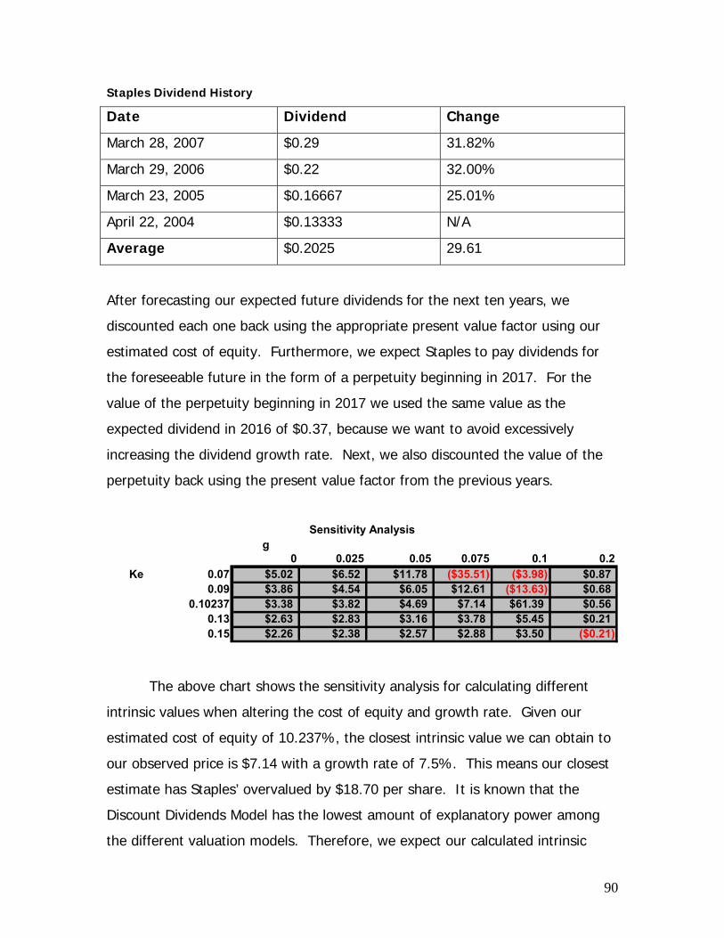
90
Staples Dividend History
Date Dividend Change
March 28, 2007 $0.29 31.82%
March 29, 2006 $0.22 32.00%
March 23, 2005 $0.16667 25.01%
April 22, 2004 $0.13333 N/A
Average $0.2025 29.61
After forecasting our expected future dividends for the next ten years, we
discounted each one back using the appropriate present value factor using our
estimated cost of equity. Furthermore, we expect Staples to pay dividends for
the foreseeable future in the form of a perpetuity beginning in 2017. For the
value of the perpetuity beginning in 2017 we used the same value as the
expected dividend in 2016 of $0.37, because we want to avoid excessively
increasing the dividend growth rate. Next, we also discounted the value of the
perpetuity back using the present value factor from the previous years.
g0 0.025 0.05 0.075 0.1 0.2
Ke 0.07 $5.02 $6.52 $11.78 ($35.51) ($3.98) $0.870.09 $3.86 $4.54 $6.05 $12.61 ($13.63) $0.68
0.10237 $3.38 $3.82 $4.69 $7.14 $61.39 $0.560.13 $2.63 $2.83 $3.16 $3.78 $5.45 $0.210.15 $2.26 $2.38 $2.57 $2.88 $3.50 ($0.21)
Sensitivity Analysis
The above chart shows the sensitivity analysis for calculating different
intrinsic values when altering the cost of equity and growth rate. Given our
estimated cost of equity of 10.237%, the closest intrinsic value we can obtain to
our observed price is $7.14 with a growth rate of 7.5%. This means our closest
estimate has Staples’ overvalued by $18.70 per share. It is known that the
Discount Dividends Model has the lowest amount of explanatory power among
the different valuation models. Therefore, we expect our calculated intrinsic

91
values using this model to contain significant error, because future dividends are
relatively difficult to accurately predict.
Discounted Free Cash Flows
The weighted average cost of capital is the discount rate used in the
discounted free cash flows model. For Staples, the WACC is 9.23%. The free
cash flows are calculated by taking the cash flows from operations and
subtracting the cash flows from investing activities. This difference is carried out
for nine of the forecasted years and is discounted each year by the discount rate.
The discount rate is computed using the formula 1/(1+WACC)t, t being the year
number in the forecast. Multiplying the free cash flows by the discount rate gives
you the present value of free cash flows. Next, we computed the perpetuity by
taking the average growth rate of the free cash flows for the forecasted years
and multiplying it by the free cash flows in the year 2015. Finally, we took the
total present value of annual cash flows and added the present value of the
terminal value to get the value of the firm. We looked at Staples’ 10-K to find the
value of debt and also discovered that they do not offer any preferred stock at
this point. After getting the book value of debt, we subtracted it from the value
of the firm to get the value of equity. We then divided the value of equity by the
number of shares outstanding to get the estimated value per share. In our
estimated value per share computations, a month is missing due to fact that the
release date for Staples’ 10-K is on March 1 and we based everything off of April
1 numbers. We simply just computed the implied value to make up for the
missing month.

92
g0 0.01 0.03 0.05
WACC 0.09 $20.13 $21.91 $27.17 $37.400.1 $17.83 $19.24 $23.25 $30.49
0.11 $15.35 $16.41 $19.33 $24.190.12 $13.30 $14.12 $16.30 $19.720.13 $11.59 $12.23 $13.89 $16.380.14 $10.15 $10.65 $11.94 $13.80
Sensitivity Analysis
The sensitivity analysis above shows that the higher the WACC is the
lower the computed share price will be. Also, as the growth rate increases and
the WACC is held constant the computed price increases. The price that is closest
to the Staples’ observed price of $25.84 on April 1, 2007 appears in the
sensitivity analysis when the WACC is at 11% and the growth rate is between
5% and 6%. Overall, with the discounted free cash flow model we decided that
the firm is overvalued in that the implied value is $20.13 and the actual price is
$25.84.
Residual Income
We placed the most emphasis for the valuation of Staples on the residual
income model because it has the largest explanatory power of the models. The
model takes the beginning book value of equity (the previous year’s ending book
value of equity), adds the annual net income, and subtracts dividends to arrive at
the ending book value of equity. Normal income (benchmark income), which is
the income you earn if you maintain value at the cost of equity, is then
computed annually by multiplying the cost of equity and the beginning book
value of equity each year. Finally, each year’s residual income is calculated by
finding the difference between the year’s net income and normal income.
Beginning in 2017 we implemented a perpetuity valued at $1,106,315, the same
value as the residual income in the previous year. We then discounted back
each year’s residual income value and the perpetuity with the appropriate
present value discount factor including the cost of equity.

93
g0 -0.1 -0.2 -0.3 -0.4 -0.5
Ke 0.07 $22.50 $17.57 $16.30 $15.71 $15.38 $15.160.09 $20.67 $17.24 $16.17 $15.66 $15.35 $15.15
0.10237 $19.90 $17.07 $16.11 $15.62 $15.33 $15.140.13 $18.72 $16.75 $15.98 $15.56 $15.30 $15.130.15 $18.14 $16.57 $15.90 $15.52 $15.29 $15.12
Sensitivity Analysis
The above chart shows the sensitivity analysis for calculating different
intrinsic values when altering the cost of equity and growth rate. Given our
estimated cost of equity of 10.237%, the closest intrinsic value we can obtain to
our observed price is $19.90 with a growth rate of 0%. This valuation implies
Staples is slightly overvalued by $5.94. We used negative growth rates because
our return on equity is significantly higher than our cost of equity, and in the
long run you ultimately earn the cost of equity. In conclusion, we found the
calculated intrinsic share price increases as the cost of equity decreases and/or
the growth rate increases.
Abnormal Earnings Growth
The abnormal earnings growth model is another significant model because
it is closely linked the residual income model. For example, the abnormal
earnings growth for year two equals the difference between residual income in
year two and residual income in year one. We have a lot of confidence in our
residual income and abnormal earning growth models because they
demonstrated this correlation with very little error, amounting to fractions of a
cent. When valuing Staples with the abnormal earnings growth model, we
began by multiplying our forecasted dividends by our cost of equity of 10.237%
and then adding that amount to Staples’ annual earnings to get cum-dividend
earnings. We then calculated our normal income, which again is the income you
earn if you maintain value at the cost of equity. To calculate normal income for
the abnormal earnings growth model we simply follow the formula:
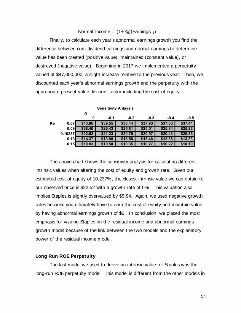
94
Normal Income = (1+KE)(Earningst-1)
Finally, to calculate each year’s abnormal earnings growth you find the
difference between cum-dividend earnings and normal earnings to determine
value has been created (positive value), maintained (constant value), or
destroyed (negative value). Beginning in 2017 we implemented a perpetuity
valued at $47,000,000, a slight increase relative to the previous year. Then, we
discounted each year’s abnormal earnings growth and the perpetuity with the
appropriate present value discount factor including the cost of equity.
g0 -0.1 -0.2 -0.3 -0.4 -0.5
Ke 0.07 $43.86 $39.55 $38.44 $37.93 $37.63 $37.440.09 $28.40 $26.43 $25.81 $25.51 $25.34 $25.22
0.10237 $22.52 $21.23 $20.79 $20.57 $20.43 $20.350.13 $14.37 $13.80 $13.58 $13.46 $13.38 $13.330.15 $10.83 $10.50 $10.35 $10.27 $10.22 $10.19
Sensitivity Anlaysis
The above chart shows the sensitivity analysis for calculating different
intrinsic values when altering the cost of equity and growth rate. Given our
estimated cost of equity of 10.237%, the closest intrinsic value we can obtain to
our observed price is $22.52 with a growth rate of 0%. This valuation also
implies Staples is slightly overvalued by $5.94. Again, we used negative growth
rates because you ultimately have to earn the cost of equity and maintain value
by having abnormal earnings growth of $0. In conclusion, we placed the most
emphasis for valuing Staples on the residual income and abnormal earnings
growth model because of the link between the two models and the explanatory
power of the residual income model.
Long Run ROE Perpetuity
The last model we used to derive an intrinsic value for Staples was the
long-run ROE perpetuity model. This model is different from the other models in

95
that it is a simple mathematical equation and not a summation of calculations
over time. The formula for this model is as follows:
P=BVE0 + BVE0 [(ROE – Ke)/(Ke – g)]
In order to obtain an intrinsic value, we first had to find the return-on-
equity for each forecasted year by simply dividing EPS for that year by the
ending BVE from the previous year. We also had to estimate a growth rate for
the book value of equity to be used in the model. We did this by taking the
difference between the average growth in the book value of equity, 16.4%, and
the cost of equity we obtained in the capital asset pricing model, 10.24%;
therefore, we used a growth rate of -6.2%. A negative growth rate was used
because growth will increase at a decreasing rate in order to level out at a point
equivalent to the cost of equity.
Sensitivity Analysis g -10% -6.2% 0 5% 10%
Ke 0.07 $11.97 $13.39 $19.01 $48.94 ($20.89) 0.09 $10.73 $11.65 $14.81 $24.51 ($62.77) 0.10237 $10.08 $10.78 $13.03 $18.74 $265.08 0.13 $8.89 $9.25 $10.29 $12.29 $20.98 0.15 $8.19 $8.39 $8.93 $9.85 $12.61
The above sensitivity analysis chart shows the different intrinsic values
calculated when altering the growth rate and the cost of equity. When using the
growth rate of -6.2% and a cost of equity of .10237, an intrinsic value of $10.78
was obtained. When adding a BVE0 of $7.00 to the resulting intrinsic value, we
obtained a final intrinsic value of $17.78. In a manner parallel to the other
valuation models, the long run ROE perpetuity model results in a slightly
overvalued market price for Staples.

96
Altman’s Z-Score/Creditworthiness
When firms obtain loans from lending companies, the lenders analyze the
firm’s creditworthiness. As valuation analysts, we too must analyze the firm’s
creditworthiness in order to gain an understanding of how firms obtain the
interest rates they receive on loans. We did this by using the Altman Z-Score
equation. This equation is a fixed weighted equation that ultimately gives a
score to a company based on numbers found in financial statements. The Z-
score equation is as follows:
Z-score = 1.2(Working Capital/Total Assets)+1.4(Retained Earnings/Total
Assets)+3.3(Earnings Before Interest and Taxes/Total Assets)+0.6(Market Value
of Equity/Book Value of Liabilities)+1.0(Sales/Total Assets)
The equation gives weights to each underlying ratio with an emphasis on
a company’s current earnings (EBIT/Total Assets). The lowest weight is given to
the market’s perception of the firm. A Z-Score of 1.8 or lower implies that a firm
has a high level of default risk, while a Z-score of 2.7 or higher implies a low
level of default risk.
Staples’ Z-scores for the previous five years are shown in the table below:
2002 2003 2004 2005 2006
Z-score 2.34 4.89 5.77 6.22 6.88
From the table above, we concluded that Staples had some credit
problems in 2002, but has increased its Z-score each year which implies Staples
is extremely creditworthy when it come to its default risk. This is important
because Staples can borrow loans with low interest premiums.

97
Valuation Conclusion
After finding the intrinsic values for each of the discount dividends,
discounted free cash flows, residual income, abnormal earnings growth, and long
run residual income perpetuity models, we found Staples’ to be overvalued. The
discount dividends model had a calculated intrinsic value of $3.38, which we
believe to be insignificant because future dividends are relatively difficult to
accurately predict. Next, the discounted free cash flows model resulted in an
intrinsic value of $20.13, implying Staples is slightly overvalued. The long run
residual income perpetuity model had an intrinsic value of $10.78 which is well
below the observed price of $25.84 at April 1, 2007. As mentioned earlier we
placed the most emphasis on the residual income and abnormal earnings growth
models; we did this because of the link between residual income and abnormal
earnings growth and the significant explanatory power of the residual income
model. The residual income model calculated an intrinsic value of $19.90,
ultimately implying that Staples is again slightly overvalued by $5.94. Lastly, the
abnormal earnings growth model computed an intrinsic value of $22.52, stating
that Staples is slightly overvalued by $3.32. Since, we placed a major emphasis
on the residual income and abnormal earnings growth models, we believe it is
safe to say Staples is a slightly overvalued firm.
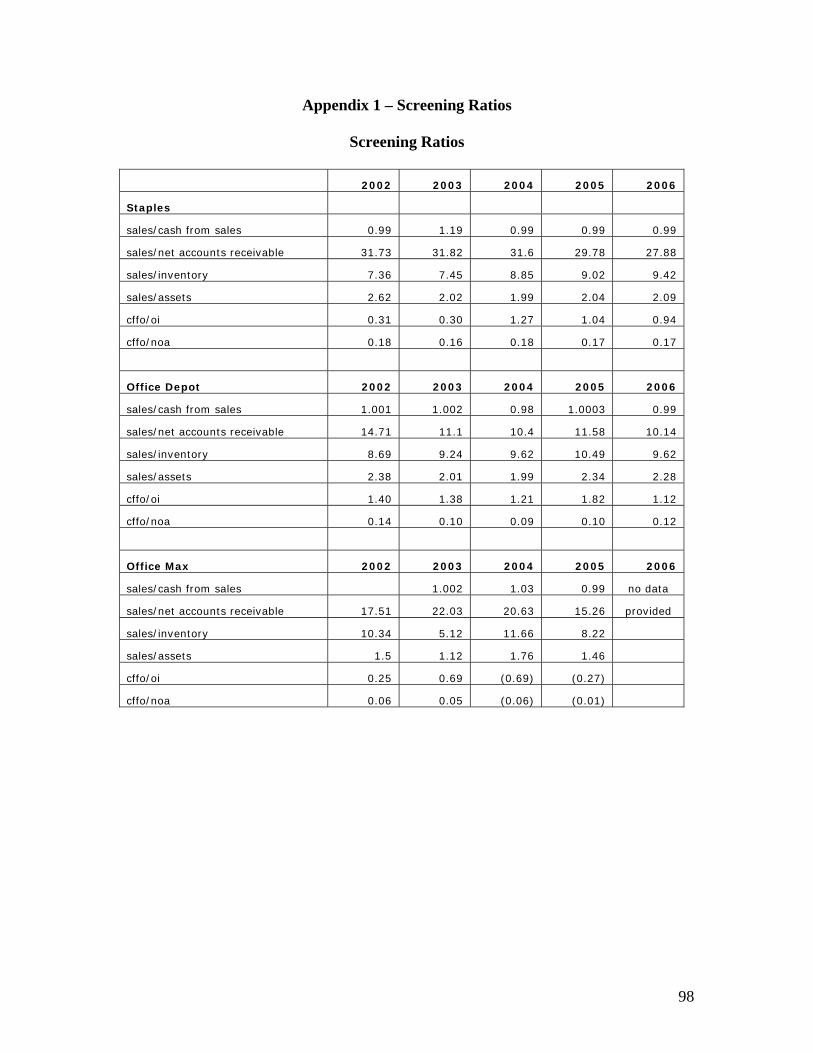
98
Appendix 1 – Screening Ratios
Screening Ratios
2002 2003 2004 2005 2006
Staples
sales/cash from sales 0.99 1.19 0.99 0.99 0.99
sales/net accounts receivable 31.73 31.82 31.6 29.78 27.88
sales/inventory 7.36 7.45 8.85 9.02 9.42
sales/assets 2.62 2.02 1.99 2.04 2.09
cffo/oi 0.31 0.30 1.27 1.04 0.94
cffo/noa 0.18 0.16 0.18 0.17 0.17
Office Depot 2002 2003 2004 2005 2006
sales/cash from sales 1.001 1.002 0.98 1.0003 0.99
sales/net accounts receivable 14.71 11.1 10.4 11.58 10.14
sales/inventory 8.69 9.24 9.62 10.49 9.62
sales/assets 2.38 2.01 1.99 2.34 2.28
cffo/oi 1.40 1.38 1.21 1.82 1.12
cffo/noa 0.14 0.10 0.09 0.10 0.12
Office Max 2002 2003 2004 2005 2006
sales/cash from sales 1.002 1.03 0.99 no data
sales/net accounts receivable 17.51 22.03 20.63 15.26 provided
sales/inventory 10.34 5.12 11.66 8.22
sales/assets 1.5 1.12 1.76 1.46
cffo/oi 0.25 0.69 (0.69) (0.27)
cffo/noa 0.06 0.05 (0.06) (0.01)

99
Appendix 2 – Core Financial Ratios
Core Financial Ratios
Current Ratio Quick Asset Ratio 2001 2002 2003 2004 2005 2006 2001 2002 2003 2004 2005 2006SPLS 1.51 1.25 1.64 1.72 1.67 1.59 SPLS 0.46 0.44 0.41 0.67 0.63 0.62ODP 1.61 1.57 1.51 1.43 1.16 ODP 0.83 0.88 0.86 0.78 0.56 OMX 1.23 1.31 1.75 1.22 1.37 OMX 0.46 0.35 1.02 0.42 0.55
Inventory Turnover Days Supply of Inventory 2001 2002 2003 2004 2005 2006 2001 2002 2003 2004 2005 2006SPLS 5.6 5.56 6.46 6.45 6.74 6.75 SPLS 65.19 65.6 56.51 56.55 54.19 54 ODP 6.14 6.35 6.61 7.27 6.63 ODP 59.4 57.49 55.24 50.22 55.05 OMX 8.36 4.12 8.99 6.11 6.09 OMX 43.67 88.62 40.59 59.74 59.9 AVG. 6.7 5.34 7.35 6.61 6.49 AVG. 56.09 70.57 50.78 55.5 56.38
Receivables Turnover Days Sales Outstanding 2001 2002 2003 2004 2005 2006 2001 2002 2003 2004 2005 2006SPLS 31.73 31.82 31.6 29.78 27.88 25.2 SPLS 11.5 11.47 11.55 12.26 13.09 14.5ODP 10.4 7.63 7.14 8.02 10.14 ODP 24.08 32.85 35.09 31.5 36 OMX 17.48 14.36 20.63 15.26 15.94 OMX 20.88 25.42 17.69 23.92 22.9 AVG. 19.87 17.94 19.79 17.69 17.99 AVG. 18.82 23.25 18.11 22.56 24
Working Capital Turnover Gross Profit Margin 2001 2002 2003 2004 2005 2006 2001 2002 2003 2004 2005 2006SPLS 13.31 21.39 9.57 9.12 9.66 11.1 SPLS 23.92 25.38 26.98 28.41 28.52 28.6ODP 9.33 9.51 10.24 13.45 30.94 ODP 29.36 31.35 31.38 30.76 31.1 OMX 30.61 13.5 9.59 25.89 15.79 OMX 19.04 19.65 22.88 25.64 27.18 AVG. 17.75 14.8 9.8 16.15 18.8 AVG 24.11 25.46 27.08 28.27 28.93
Operating Expense Ratio Net Profit Margin 2001 2002 2003 2004 2005 2006 2001 2002 2003 2004 2005 2006SPLS 18.91 19.4 20.76 20.56 20.27 20.5 SPLS 2.47 3.85 3.78 4.9 5.19 5.36ODP 24.87 27.4 27.21 27.39 26.3 ODP 2.74 2.21 2.47 1.92 3.44 OMX 12.68 13.44 15.14 23.89 23.91 OMX 0.15 0.1 1.3 -0.81 1.02 AVG. 18.82 20.08 21.04 23.95 23.5 AVG. 1.79 2.05 2.52 2 3.22
Asset Turnover Return on Assets 2001 2002 2003 2004 2005 2006 2002 2003 2004 2005 2006
SPLS 2.63 2.03 1.99 2.04 2.09 2.16 SPLS 10.90% 8.57% 10.89% 11.80% 12.68% ODP 2.38 2.01 2.1 2.34 2.28 ODP 0.06 0.05 0.04 0.08 OMX 1.49 1.12 1.73 1.46 1.44 OMX 0.01 0.01 0.02 0 AVG. 2.17 1.72 1.94 1.95 1.94 2.16 AVG. 3.66 2.88 3.65 3.96 12.68
Debt to Equity Ratio Return on Equity Year 2001 2002 2003 2004 2005 2006 2002 2003 2004 2005 2006 SPLS 0.91 1.03 1.23 1.25 1.28 1.42 SPLS 21.72 18.44 19.34 20.28 22 ODP 1.07 1.19 1.11 1.23 1.52 ODP 0.11 0.12 0.09 0.19 OMX 2.53 2.17 1.93 2.61 2.13 OMX 0.05 -0.02 0.07 0.01 AVG. 1.5 1.46 1.42 1.7 1.64 1.42 AVG. 7.29 6.18 6.5 6.83 22
Times Interest Earned Debt Service Margin Year 2001 2002 2003 2004 2005 2006 Year 2001 2002 2003 2004 2005 SPLS 16.83 33.12 25.28 28.23 23.13 30.6 SPLS 154.71 2.79 5.36 947.92 427.32 ODP 10.37 8.04 7.55 11.16 17.81 ODP 17.18 13.45 1.11 0.79 1.7 OMX 0.01 0.37 2.49 0.29 1.39 OMX 14.66 -0.66 -4.17 3.68 2.22 AVG. 9.07 13.84 11.77 13.23 14.11 30.6 AVG. 62.18 5.19 0.77 317.46 143.75
SGR Ratios IGR Ratios 2003 2004 2005 2006 2003 2004 2005 2006
SPLS -
4.24% 5.06% 8.07% 8.59% SPLS 28 22.5 28.7 32.4
ODP -
0.01% -
0.01% -
0.01% -
0.04% ODP 0.06 0.05 0.04 0.08
OMX 0.01% -
0.01% 0.03% -
0.01% OMX -0.01 0.02 -0.02 0.01
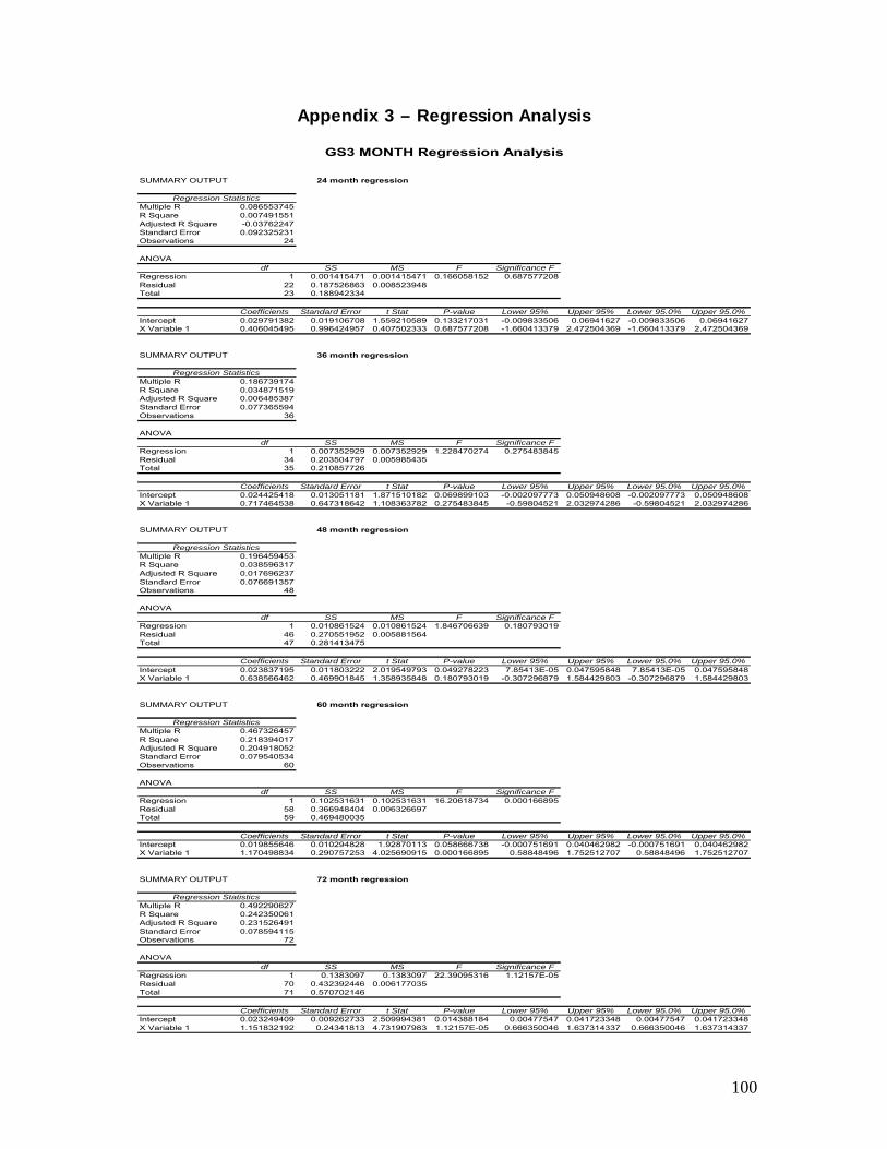
100
Appendix 3 – Regression Analysis
SUMMARY OUTPUT
Regression StatisticsMultiple R 0.086553745R Square 0.007491551Adjusted R Square -0.03762247Standard Error 0.092325231Observations 24
ANOVAdf SS MS F Significance F
Regression 1 0.001415471 0.001415471 0.166058152 0.687577208Residual 22 0.187526863 0.008523948Total 23 0.188942334
Coefficients Standard Error t Stat P-value Lower 95% Upper 95% Lower 95.0% Upper 95.0%Intercept 0.029791382 0.019106708 1.559210589 0.133217031 -0.009833506 0.06941627 -0.009833506 0.06941627X Variable 1 0.406045495 0.996424957 0.407502333 0.687577208 -1.660413379 2.472504369 -1.660413379 2.472504369
SUMMARY OUTPUT
Regression StatisticsMultiple R 0.186739174R Square 0.034871519Adjusted R Square 0.006485387Standard Error 0.077365594Observations 36
ANOVAdf SS MS F Significance F
Regression 1 0.007352929 0.007352929 1.228470274 0.275483845Residual 34 0.203504797 0.005985435Total 35 0.210857726
Coefficients Standard Error t Stat P-value Lower 95% Upper 95% Lower 95.0% Upper 95.0%Intercept 0.024425418 0.013051181 1.871510182 0.069899103 -0.002097773 0.050948608 -0.002097773 0.050948608X Variable 1 0.717464538 0.647318642 1.108363782 0.275483845 -0.59804521 2.032974286 -0.59804521 2.032974286
SUMMARY OUTPUT
Regression StatisticsMultiple R 0.196459453R Square 0.038596317Adjusted R Square 0.017696237Standard Error 0.076691357Observations 48
ANOVAdf SS MS F Significance F
Regression 1 0.010861524 0.010861524 1.846706639 0.180793019Residual 46 0.270551952 0.005881564Total 47 0.281413475
Coefficients Standard Error t Stat P-value Lower 95% Upper 95% Lower 95.0% Upper 95.0%Intercept 0.023837195 0.011803222 2.019549793 0.049278223 7.85413E-05 0.047595848 7.85413E-05 0.047595848X Variable 1 0.638566462 0.469901845 1.358935848 0.180793019 -0.307296879 1.584429803 -0.307296879 1.584429803
SUMMARY OUTPUT
Regression StatisticsMultiple R 0.467326457R Square 0.218394017Adjusted R Square 0.204918052Standard Error 0.079540534Observations 60
ANOVAdf SS MS F Significance F
Regression 1 0.102531631 0.102531631 16.20618734 0.000166895Residual 58 0.366948404 0.006326697Total 59 0.469480035
Coefficients Standard Error t Stat P-value Lower 95% Upper 95% Lower 95.0% Upper 95.0%Intercept 0.019855646 0.010294828 1.92870113 0.058666738 -0.000751691 0.040462982 -0.000751691 0.040462982X Variable 1 1.170498834 0.290757253 4.025690915 0.000166895 0.58848496 1.752512707 0.58848496 1.752512707
SUMMARY OUTPUT
Regression StatisticsMultiple R 0.492290627R Square 0.242350061Adjusted R Square 0.231526491Standard Error 0.078594115Observations 72
ANOVAdf SS MS F Significance F
Regression 1 0.1383097 0.1383097 22.39095316 1.12157E-05Residual 70 0.432392446 0.006177035Total 71 0.570702146
Coefficients Standard Error t Stat P-value Lower 95% Upper 95% Lower 95.0% Upper 95.0%Intercept 0.023249409 0.009262733 2.509994381 0.014388184 0.00477547 0.041723348 0.00477547 0.041723348X Variable 1 1.151832192 0.24341813 4.731907983 1.12157E-05 0.666350046 1.637314337 0.666350046 1.637314337
60 month regression
72 month regression
GS3 MONTH Regression Analysis
24 month regression
36 month regression
48 month regression
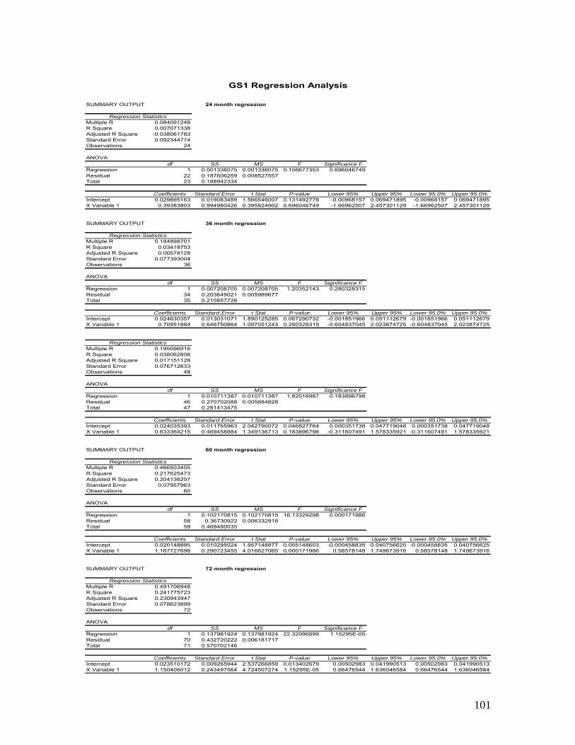
101
SUMMARY OUTPUT
Regression StatisticsMultiple R 0.084091248R Square 0.007071338Adjusted R Square -0.038061783Standard Error 0.092344774Observations 24
ANOVAdf SS MS F Significance F
Regression 1 0.001336075 0.001336075 0.156677353 0.696046749Residual 22 0.187606259 0.008527557Total 23 0.188942334
Coefficients Standard Error t Stat P-value Lower 95% Upper 95% Lower 95.0% Upper 95.0%Intercept 0.029895163 0.019083489 1.566546007 0.131492778 -0.00968157 0.069471895 -0.00968157 0.069471895X Variable 1 0.39383803 0.994980426 0.395824902 0.696046749 -1.66962507 2.457301129 -1.66962507 2.457301129
SUMMARY OUTPUT
Regression StatisticsMultiple R 0.184898701R Square 0.03418753Adjusted R Square 0.00578128Standard Error 0.077393004Observations 36
ANOVAdf SS MS F Significance F
Regression 1 0.007208705 0.007208705 1.20352143 0.280328315Residual 34 0.203649021 0.005989677Total 35 0.210857726
Coefficients Standard Error t Stat P-value Lower 95% Upper 95% Lower 95.0% Upper 95.0%Intercept 0.024630357 0.013031071 1.890125285 0.067290732 -0.001851966 0.051112679 -0.001851966 0.051112679X Variable 1 0.70951884 0.646750864 1.097051243 0.280328315 -0.604837045 2.023874725 -0.604837045 2.023874725
Regression StatisticsMultiple R 0.195096916R Square 0.038062806Adjusted R Square 0.017151128Standard Error 0.076712633Observations 48
ANOVAdf SS MS F Significance F
Regression 1 0.010711387 0.010711387 1.82016987 0.183896798Residual 46 0.270702088 0.005884828Total 47 0.281413475
Coefficients Standard Error t Stat P-value Lower 95% Upper 95% Lower 95.0% Upper 95.0%Intercept 0.024035393 0.011765963 2.042790072 0.046827764 0.000351738 0.047719048 0.000351738 0.047719048X Variable 1 0.633364215 0.469458884 1.349136713 0.183896798 -0.311607491 1.578335921 -0.311607491 1.578335921
SUMMARY OUTPUT
Regression StatisticsMultiple R 0.466503455R Square 0.217625473Adjusted R Square 0.204136257Standard Error 0.07957963Observations 60
ANOVAdf SS MS F Significance F
Regression 1 0.102170815 0.102170815 16.13329298 0.000171986Residual 58 0.36730922 0.006332918Total 59 0.469480035
Coefficients Standard Error t Stat P-value Lower 95% Upper 95% Lower 95.0% Upper 95.0%Intercept 0.020148895 0.010295024 1.957148877 0.055148603 -0.000458835 0.040756625 -0.000458835 0.040756625X Variable 1 1.167727698 0.290723455 4.016627065 0.000171986 0.58578148 1.749673916 0.58578148 1.749673916
SUMMARY OUTPUT
Regression StatisticsMultiple R 0.491706948R Square 0.241775723Adjusted R Square 0.230943947Standard Error 0.078623899Observations 72
ANOVAdf SS MS F Significance F
Regression 1 0.137981924 0.137981924 22.32096899 1.15295E-05Residual 70 0.432720222 0.006181717Total 71 0.570702146
Coefficients Standard Error t Stat P-value Lower 95% Upper 95% Lower 95.0% Upper 95.0%Intercept 0.023510172 0.009265944 2.537266859 0.013402679 0.00502983 0.041990513 0.00502983 0.041990513X Variable 1 1.150406012 0.243497564 4.724507274 1.15295E-05 0.66476544 1.636046584 0.66476544 1.636046584
60 month regression
72 month regression
GS1 Regression Analysis
24 month regression
36 month regression
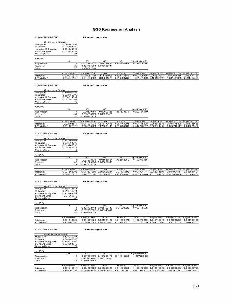
102
SUMMARY OUTPUT
Regression StatisticsMultiple R 0.078240898R Square 0.006121638Adjusted R Square -0.039054651Standard Error 0.092388925Observations 24
ANOVAdf SS MS F Significance F
Regression 1 0.001156637 0.001156637 0.135505554 0.716308786Residual 22 0.187785698 0.008535714Total 23 0.188942334
Coefficients Standard Error t Stat P-value Lower 95% Upper 95% Lower 95.0% Upper 95.0%Intercept 0.029989514 0.019087403 1.571167905 0.130415889 -0.009595336 0.069574364 -0.009595336 0.069574364X Variable 1 0.365018108 0.991598502 0.36811079 0.716308786 -1.691431309 2.421467525 -1.691431309 2.421467525
SUMMARY OUTPUT
Regression StatisticsMultiple R 0.180995283R Square 0.032759293Adjusted R Square 0.004311037Standard Error 0.077450207Observations 36
ANOVAdf SS MS F Significance F
Regression 1 0.00690755 0.00690755 1.151539572 0.290784669Residual 34 0.203950176 0.005998535Total 35 0.210857726
Coefficients Standard Error t Stat P-value Lower 95% Upper 95% Lower 95.0% Upper 95.0%Intercept 0.02495544 0.013005939 1.918772645 0.063440204 -0.001475808 0.051386688 -0.001475808 0.051386688X Variable 1 0.691137673 0.644058228 1.073098118 0.290784669 -0.617746117 2.000021462 -0.617746117 2.000021462
SUMMARY OUTPUT
Regression StatisticsMultiple R 0.192104667R Square 0.036904203Adjusted R Square 0.015967338Standard Error 0.076758817Observations 48
ANOVAdf SS MS F Significance F
Regression 1 0.01038534 0.01038534 1.762642259 0.190846455Residual 46 0.271028135 0.005891916Total 47 0.281413475
Coefficients Standard Error t Stat P-value Lower 95% Upper 95% Lower 95.0% Upper 95.0%Intercept 0.024506308 0.011677304 2.098627214 0.04136892 0.001001114 0.048011501 0.001001114 0.048011501X Variable 1 0.626770273 0.472091631 1.327645381 0.190846455 -0.323500878 1.577041424 -0.323500878 1.577041424
SUMMARY OUTPUT
Regression StatisticsMultiple R 0.465478647R Square 0.216670371Adjusted R Square 0.203164687Standard Error 0.07962819Observations 60
ANOVAdf SS MS F Significance F
Regression 1 0.101722413 0.101722413 16.04290329 0.000178525Residual 58 0.367757622 0.006340649Total 59 0.469480035
Coefficients Standard Error t Stat P-value Lower 95% Upper 95% Lower 95.0% Upper 95.0%Intercept 0.021111325 0.010288698 2.051894647 0.044703476 0.000516258 0.041706392 0.000516258 0.041706392X Variable 1 1.163265806 0.290427328 4.005359321 0.000178525 0.58191235 1.744619261 0.58191235 1.744619261
SUMMARY OUTPUT
Regression StatisticsMultiple R 0.490376394R Square 0.240469008Adjusted R Square 0.229618565Standard Error 0.078691619Observations 72
ANOVAdf SS MS F Significance F
Regression 1 0.137236179 0.137236179 22.16213784 1.22758E-05Residual 70 0.433465967 0.006192371Total 71 0.570702146
Coefficients Standard Error t Stat P-value Lower 95% Upper 95% Lower 95.0% Upper 95.0%Intercept 0.024515644 0.009275855 2.642952503 0.010133685 0.006015535 0.043015753 0.006015535 0.043015753X Variable 1 1.146067639 0.243446998 4.707667983 1.22758E-05 0.660527917 1.631607361 0.660527917 1.631607361
60 month regression
72 month regression
GS5 Regression Analysis
24 month regression
36 month regression
48 month regression

103
SUMMARY OUTPUT
Regression StatisticsMultiple R 0.07724672R Square 0.005967056Adjusted R Square -0.03921626Standard Error 0.09239611Observations 24
ANOVAdf SS MS F Significance F
Regression 1 0.001127429 0.001127429 0.132063254 0.719770993Residual 22 0.187814905 0.008537041Total 23 0.188942334
Coefficients Standard Error t Stat P-value Lower 95% Upper 95% Lower 95.0% Upper 95.0%Intercept 0.030015554 0.019083709 1.572836467 0.13002892 -0.009561637 0.069592744 -0.009561637 0.069592744X Variable 1 0.360166888 0.991089299 0.363405083 0.719770993 -1.695226506 2.415560283 -1.695226506 2.415560283
SUMMARY OUTPUT
Regression StatisticsMultiple R 0.180522947R Square 0.032588534Adjusted R Square 0.004135256Standard Error 0.077457043Observations 36
ANOVAdf SS MS F Significance F
Regression 1 0.006871544 0.006871544 1.145334958 0.292066719Residual 34 0.203986182 0.005999594Total 35 0.210857726
Coefficients Standard Error t Stat P-value Lower 95% Upper 95% Lower 95.0% Upper 95.0%Intercept 0.025051071 0.012996946 1.927458297 0.062310959 -0.001361901 0.051464042 -0.001361901 0.051464042X Variable 1 0.68862421 0.643451813 1.070203232 0.292066719 -0.619027196 1.996275616 -0.619027196 1.996275616
SUMMARY OUTPUT
Regression StatisticsMultiple R 0.19176517R Square 0.03677388Adjusted R Square 0.015834182Standard Error 0.07676401Observations 48
ANOVAdf SS MS F Significance F
Regression 1 0.010348665 0.010348665 1.756180052 0.191646605Residual 46 0.27106481 0.005892713Total 47 0.281413475
Coefficients Standard Error t Stat P-value Lower 95% Upper 95% Lower 95.0% Upper 95.0%Intercept 0.02463916 0.011648824 2.115162905 0.039862961 0.001191294 0.048087026 0.001191294 0.048087026X Variable 1 0.626771553 0.472960375 1.325209437 0.191646605 -0.32524829 1.578791395 -0.32524829 1.578791395
SUMMARY OUTPUT
Regression StatisticsMultiple R 0.465417422R Square 0.216613377Adjusted R Square 0.203106711Standard Error 0.079631087Observations 60
ANOVAdf SS MS F Significance F
Regression 1 0.101695656 0.101695656 16.03751645 0.000178922Residual 58 0.367784379 0.00634111Total 59 0.469480035
Coefficients Standard Error t Stat P-value Lower 95% Upper 95% Lower 95.0% Upper 95.0%Intercept 0.021407622 0.010286291 2.081180003 0.04184229 0.000817375 0.04199787 0.000817375 0.04199787X Variable 1 1.163008089 0.290411746 4.00468681 0.000178922 0.581685824 1.744330353 0.581685824 1.744330353
SUMMARY OUTPUT
Regression StatisticsMultiple R 0.490249418R Square 0.240344492Adjusted R Square 0.229492271Standard Error 0.078698069Observations 72
ANOVAdf SS MS F Significance F
Regression 1 0.137165117 0.137165117 22.14703149 1.23493E-05Residual 70 0.433537029 0.006193386Total 71 0.570702146
Coefficients Standard Error t Stat P-value Lower 95% Upper 95% Lower 95.0% Upper 95.0%Intercept 0.024815209 0.009278143 2.674587924 0.009306893 0.006310537 0.043319881 0.006310537 0.043319881X Variable 1 1.145733221 0.24345895 4.706063269 1.23493E-05 0.660169663 1.631296779 0.660169663 1.631296779
60 month regression
72 month regression
GS 7 Regression Analysis
24 month regression
36 month regression
48 month regression
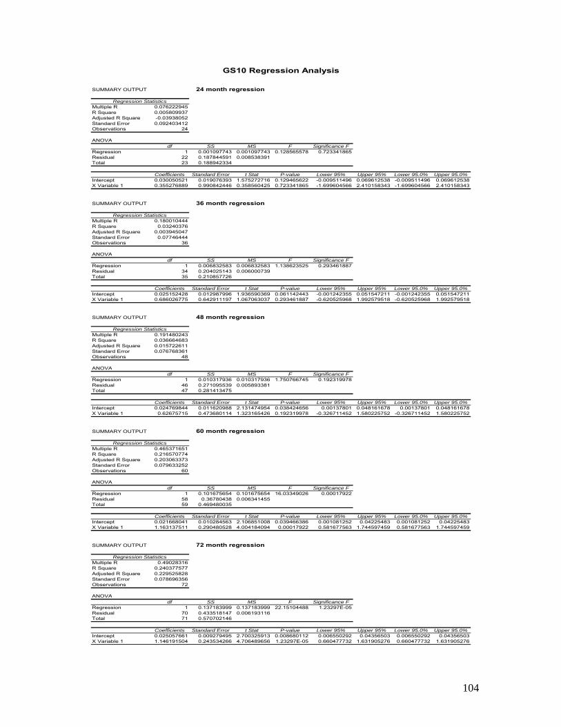
104
SUMMARY OUTPUT
Regression StatisticsMultiple R 0.076222945R Square 0.005809937Adjusted R Square -0.03938052Standard Error 0.092403412Observations 24
ANOVAdf SS MS F Significance F
Regression 1 0.001097743 0.001097743 0.128565578 0.723341865Residual 22 0.187844591 0.008538391Total 23 0.188942334
Coefficients Standard Error t Stat P-value Lower 95% Upper 95% Lower 95.0% Upper 95.0%Intercept 0.030050521 0.019076393 1.575272716 0.129465622 -0.009511496 0.069612538 -0.009511496 0.069612538X Variable 1 0.355276889 0.990842446 0.358560425 0.723341865 -1.699604566 2.410158343 -1.699604566 2.410158343
SUMMARY OUTPUT
Regression StatisticsMultiple R 0.180010444R Square 0.03240376Adjusted R Square 0.003945047Standard Error 0.07746444Observations 36
ANOVAdf SS MS F Significance F
Regression 1 0.006832583 0.006832583 1.138623525 0.293461887Residual 34 0.204025143 0.006000739Total 35 0.210857726
Coefficients Standard Error t Stat P-value Lower 95% Upper 95% Lower 95.0% Upper 95.0%Intercept 0.025152428 0.012987996 1.936590369 0.061142443 -0.001242355 0.051547211 -0.001242355 0.051547211X Variable 1 0.686026775 0.642911197 1.067063037 0.293461887 -0.620525968 1.992579518 -0.620525968 1.992579518
SUMMARY OUTPUT
Regression StatisticsMultiple R 0.191480243R Square 0.036664683Adjusted R Square 0.015722611Standard Error 0.076768361Observations 48
ANOVAdf SS MS F Significance F
Regression 1 0.010317936 0.010317936 1.750766745 0.192319978Residual 46 0.271095539 0.005893381Total 47 0.281413475
Coefficients Standard Error t Stat P-value Lower 95% Upper 95% Lower 95.0% Upper 95.0%Intercept 0.024769844 0.011620988 2.131474954 0.038424656 0.00137801 0.048161678 0.00137801 0.048161678X Variable 1 0.62675715 0.473680114 1.323165426 0.192319978 -0.326711452 1.580225752 -0.326711452 1.580225752
SUMMARY OUTPUT
Regression StatisticsMultiple R 0.465371651R Square 0.216570774Adjusted R Square 0.203063373Standard Error 0.079633252Observations 60
ANOVAdf SS MS F Significance F
Regression 1 0.101675654 0.101675654 16.03349026 0.00017922Residual 58 0.36780438 0.006341455Total 59 0.469480035
Coefficients Standard Error t Stat P-value Lower 95% Upper 95% Lower 95.0% Upper 95.0%Intercept 0.021668041 0.010284563 2.106851008 0.039466386 0.001081252 0.04225483 0.001081252 0.04225483X Variable 1 1.163137511 0.290480528 4.004184094 0.00017922 0.581677563 1.744597459 0.581677563 1.744597459
SUMMARY OUTPUT
Regression StatisticsMultiple R 0.49028316R Square 0.240377577Adjusted R Square 0.229525828Standard Error 0.078696356Observations 72
ANOVAdf SS MS F Significance F
Regression 1 0.137183999 0.137183999 22.15104488 1.23297E-05Residual 70 0.433518147 0.006193116Total 71 0.570702146
Coefficients Standard Error t Stat P-value Lower 95% Upper 95% Lower 95.0% Upper 95.0%Intercept 0.025057661 0.009279495 2.700325913 0.008680112 0.006550292 0.04356503 0.006550292 0.04356503X Variable 1 1.146191504 0.243534266 4.706489656 1.23297E-05 0.660477732 1.631905276 0.660477732 1.631905276
72 month regression
GS10 Regression Analysis
24 month regression
36 month regression
48 month regression
60 month regression
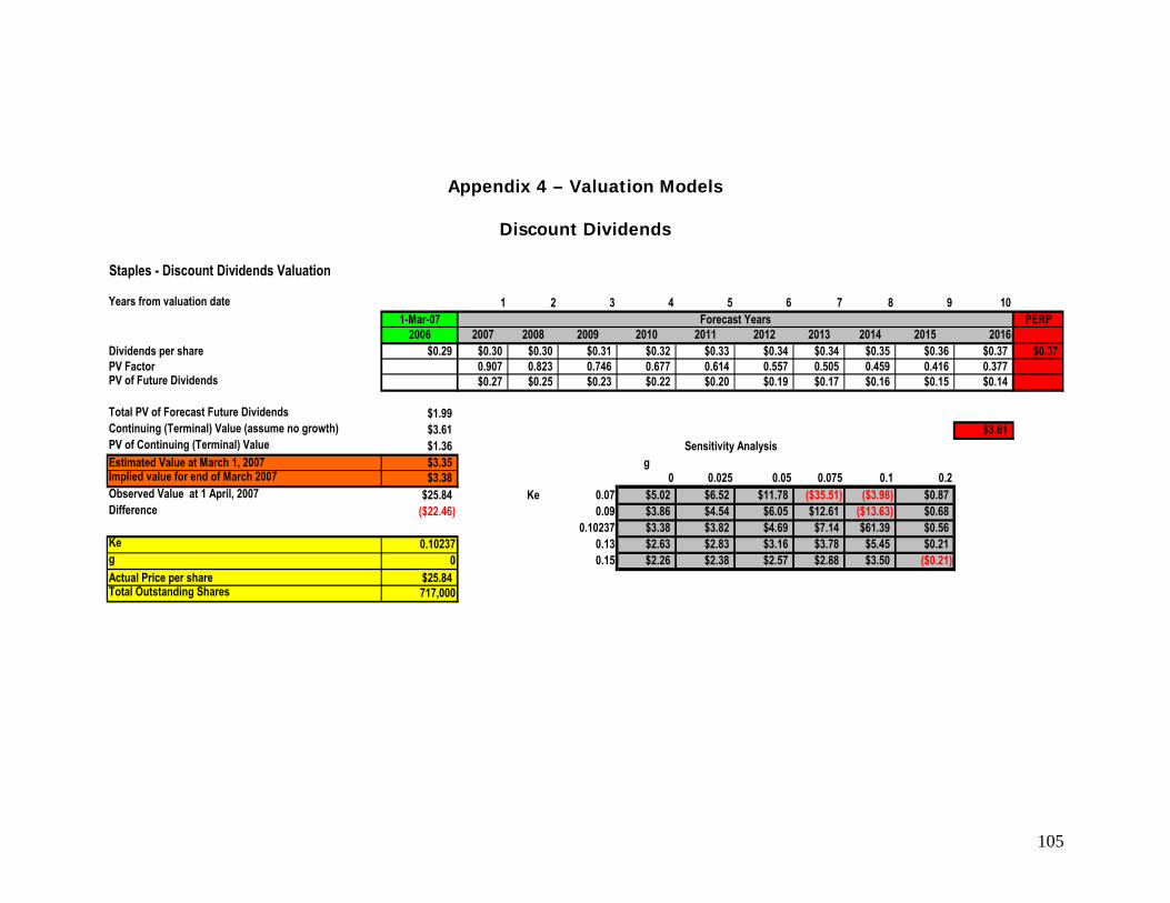
105
Appendix 4 – Valuation Models
Discount Dividends
Staples - Discount Dividends Valuation
Years from valuation date 1 2 3 4 5 6 7 8 9 101-Mar-07 PERP
2006 2007 2008 2009 2010 2011 2012 2013 2014 2015 2016Dividends per share $0.29 $0.30 $0.30 $0.31 $0.32 $0.33 $0.34 $0.34 $0.35 $0.36 $0.37 $0.37PV Factor 0.907 0.823 0.746 0.677 0.614 0.557 0.505 0.459 0.416 0.377PV of Future Dividends $0.27 $0.25 $0.23 $0.22 $0.20 $0.19 $0.17 $0.16 $0.15 $0.14
Total PV of Forecast Future Dividends $1.99Continuing (Terminal) Value (assume no growth) $3.61 $3.61PV of Continuing (Terminal) Value $1.36Estimated Value at March 1, 2007 $3.35 gImplied value for end of March 2007 $3.38 0 0.025 0.05 0.075 0.1 0.2Observed Value at 1 April, 2007 $25.84 Ke 0.07 $5.02 $6.52 $11.78 ($35.51) ($3.98) $0.87Difference ($22.46) 0.09 $3.86 $4.54 $6.05 $12.61 ($13.63) $0.68
0.10237 $3.38 $3.82 $4.69 $7.14 $61.39 $0.56Ke 0.10237 0.13 $2.63 $2.83 $3.16 $3.78 $5.45 $0.21g 0 0.15 $2.26 $2.38 $2.57 $2.88 $3.50 ($0.21)Actual Price per share $25.84Total Outstanding Shares 717,000
Forecast Years
Sensitivity Analysis

106
Discounted Free Cash Flows
Staples - Discounted Free Cash Flows1 2 3 4 5 6 7 8 9
Forecasted Years PERP1-Mar-07 2007 2008 2009 2010 2011 2012 2013 2014 2015
Cash Flow from Operations $1,275,464,907 $1,396,417,244 $1,528,839,491 $1,673,819,340 $1,832,547,628 $2,006,328,120 $2,196,588,215 $2,404,890,676 $2,632,946,459Cash Provided (Used) by Investing Activities ($440,000,000) ($468,986,939) ($520,575,503) ($577,838,808) ($641,401,077) ($550,147,196) ($596,909,708) ($647,647,033) ($702,697,031)Free Cash Flow (to firm) $835,464,907 $927,430,305 $1,008,263,989 $1,095,980,532 $1,191,146,552 $1,456,180,924 $1,599,678,507 $1,757,243,643 $1,930,249,428 $2,123,274,371Discount Rate (9% WACC) 0.916 0.838 0.767 0.702 0.643 0.589 0.539 0.494 0.452Present Value of Free Cash Flows $764,873,227 $777,327,043 $773,673,992 $769,923,948 $766,075,253 $857,398,699 $862,306,063 $867,205,369 $872,096,727Total Present Value of Annual Cash Flows $7,310,880,321
Continuing (Terminal) Value (assume no growth) $23,006,050,046 $23,006,050,046Present Value of Continuing (Terminal) Value $10,394,253,020 Sensitivity AnalysisValue of the Firm (end of 2006) $17,705,133,341 gBook Value of Debt $3,375,600,000 0 0.01 0.03 0.05Value of Equity (end of 2006) $14,329,533,341 WACC 0.09 $20.13 $21.91 $27.17 $37.40Estimated Value per Share at March 1, 2007 19.99 0.1 $17.83 $19.24 $23.25 $30.49Implied value for end of March 2007 20.13 0.11 $15.35 $16.41 $19.33 $24.19Actual Price per share $25.84 0.12 $13.30 $14.12 $16.30 $19.72Difference ($5.71) 0.13 $11.59 $12.23 $13.89 $16.38
0.14 $10.15 $10.65 $11.94 $13.80WACC 0.09g 0.00Actual Price per share $25.84Total Outstanding Shares 717000

107
Residual Income Staples-Residual Income
Years from valuation date 0 1 2 3 4 5 6 7 8 9 101-Mar-07 Forecast Years PERP
2006 2007 2008 2009 2010 2011 2012 2013 2014 2015 2016Beginning BE $5,021,665 $5,919,556 $6,967,894 $8,187,375 $9,601,386 $11,236,349 $13,074,204 $15,136,783 $17,448,143 $20,034,784Earnings $1,111,019 $1,266,795 $1,443,399 $1,643,526 $1,870,217 $2,078,990 $2,309,743 $2,564,702 $2,846,317 $3,157,276Dividends $213,128 $218,456 $223,918 $229,516 $235,254 $241,135 $247,163 $253,343 $259,676 $266,168Ending BE $5,021,665 $5,919,556 $6,967,894 $8,187,375 $9,601,386 $11,236,349 $13,074,204 $15,136,783 $17,448,143 $20,034,784 $22,925,892Ke 0.10237"Normal" Income $514,068 $605,985 $713,303 $838,142 $982,894 $1,150,265 $1,338,406 $1,549,553 $1,786,166 $2,050,961Residual Income (RI) $596,951 $660,810 $730,096 $805,384 $887,323 $928,725 $971,337 $1,015,149 $1,060,151 $1,106,315 $1,106,315
Discount Factor 0.907 0.823 0.746 0.677 0.614 0.557 0.505 0.459 0.416 0.377Present Value of RI $541,516.15 $543,778.32 $545,001.39 $545,373 $545,061 $517,515 $490,996 $465,491 $440,982 $417,451∆ Residual Income $63,858.92 $69,285.58 $75,289 $81,939 $41,402 $42,612 $43,813 $45,001 $46,165ROE 22.12% 21.40% 20.71% 20.07% 19.48% 18.50% 17.67% 16.94% 16.31% 15.76% Avg. ROE 18.90%ROE Growth -3.3% -3.2% -3.1% -3.0% -5.0% -4.5% -4.1% -3.7% -3.4% Avg. ROE Growth -3.7%BV Equity (per share) 2006 $7.00Total PV of RI (end 2006) $7.05Continuation (Terminal) Value $15.07 $10,807,025.29PV of Terminal Value (end 2006) $5.69Estimated Value at March 1, 2007 $19.74 gImplied value for end of March 2007 $19.90 0 -0.1 -0.2 -0.3 -0.4 -0.5Observed Value at 1 April, 2007 $25.84 Ke 0.07 $22.50 $17.57 $16.30 $15.71 $15.38 $15.16Difference ($5.94) 0.09 $20.67 $17.24 $16.17 $15.66 $15.35 $15.15
0.10237 $19.90 $17.07 $16.11 $15.62 $15.33 $15.14Ke 0.10237 0.13 $18.72 $16.75 $15.98 $15.56 $15.30 $15.13Growth 0 0.15 $18.14 $16.57 $15.90 $15.52 $15.29 $15.12Actual Price per share $25.84Total Outstanding Shares 717000
Sensitivity Analysis

108
Abnormal Earnings Growth
Years from valuation date 0 1 2 3 4 5 6 7 8 91-Mar-07 Forecast Years PERP
2006 2007 2008 2009 2010 2011 2012 2013 2014 2015 2016Earnings $1,111,019 $1,266,795 $1,443,399 $1,643,526 $1,870,217 $2,078,990 $2,309,743 $2,564,702 $2,846,317 $3,157,276Dividends $213,128 $218,456 $223,918 $229,516 $235,254 $241,135 $247,163 $253,343 $259,676 $266,168Dividends invested at 10.237% (Drip) $21,818 $22,363 $22,922 $23,496 $24,083 $24,685 $25,302 $25,935 $26,583Cum-Dividend Earnings $1,288,613 $1,465,762 $1,666,448 $1,893,713 $2,103,073 $2,334,428 $2,590,004 $2,872,252 $3,183,859Normal Earnings $1,224,754 $1,396,477 $1,591,160 $1,811,774 $2,061,671 $2,291,816 $2,546,191 $2,827,251 $3,137,694Abnormal Earning Growth (AEG) $63,859 $69,286 $75,289 $81,939 $41,402 $42,612 $43,813 $45,001 $46,165 $47,000
PV Factor 0.91 0.82 0.75 0.68 0.61 0.56 0.51 0.46 0.42PV of AEG $57,929 $57,015 $56,201 $55,486 $25,432 $23,745 $22,147 $20,635 $19,203
Residual Income Difference $63,858.92 $69,285.58 $75,288.72 $81,938.78 $41,401.81 $42,611.79 $43,812.73 $45,001.13 $46,164.57Error $0.00 $0.00 $0.00 $0.00 $0.00 $0.00 $0.00 $0.00 $0.00
Core EPS $1.55Total PV of AEG $0.47Continuing (Terminal) Value $0.07 $459,119PV of Terminal Value $0.27Total PV of AEG $0.74 gTotal Average EPS Perp (t+1) $2.29 0 -0.1 -0.2 -0.3 -0.4 -0.5Capitalization Rate (perpetuity) 0.10237 Ke 0.07 $43.86 $39.55 $38.44 $37.93 $37.63 $37.44Estimated Value at March 1, 2007 $22.34 0.09 $28.40 $26.43 $25.81 $25.51 $25.34 $25.22Implied Value for end of March 2007 $22.52 0.10237 $22.52 $21.23 $20.79 $20.57 $20.43 $20.35Observed Value at 1 April, 2007 $25.84 0.13 $14.37 $13.80 $13.58 $13.46 $13.38 $13.33Difference ($3.32) 0.15 $10.83 $10.50 $10.35 $10.27 $10.22 $10.19
Ke 0.10237g 0Actual Price per share $25.84Total Outstanding Shares 717000
Staples - Abnormal Earnings Growth
Sensitivity Anlaysis
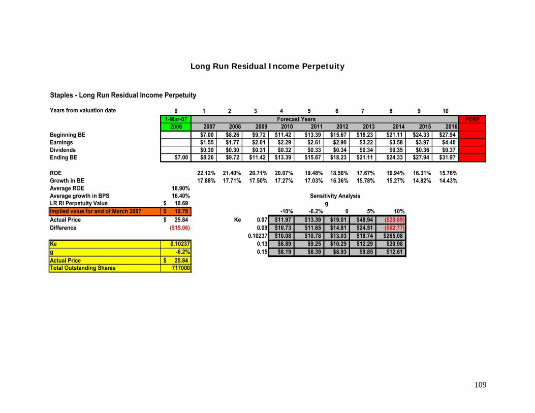
109
Long Run Residual Income Perpetuity
Staples - Long Run Residual Income Perpetuity
Years from valuation date 0 1 2 3 4 5 6 7 8 9 101-Mar-07 PERP
2006 2007 2008 2009 2010 2011 2012 2013 2014 2015 2016Beginning BE $7.00 $8.26 $9.72 $11.42 $13.39 $15.67 $18.23 $21.11 $24.33 $27.94Earnings $1.55 $1.77 $2.01 $2.29 $2.61 $2.90 $3.22 $3.58 $3.97 $4.40Dividends $0.30 $0.30 $0.31 $0.32 $0.33 $0.34 $0.34 $0.35 $0.36 $0.37Ending BE $7.00 $8.26 $9.72 $11.42 $13.39 $15.67 $18.23 $21.11 $24.33 $27.94 $31.97
ROE 22.12% 21.40% 20.71% 20.07% 19.48% 18.50% 17.67% 16.94% 16.31% 15.76%Growth in BE 17.88% 17.71% 17.50% 17.27% 17.03% 16.36% 15.78% 15.27% 14.82% 14.43%Average ROE 18.90%Average growth in BPS 16.40%LR RI Perpetuity Value 10.69$ gImplied value for end of March 2007 10.78$ -10% -6.2% 0 5% 10%Actual Price 25.84$ Ke 0.07 $11.97 $13.39 $19.01 $48.94 ($20.89)Difference ($15.06) 0.09 $10.73 $11.65 $14.81 $24.51 ($62.77)
0.10237 $10.08 $10.78 $13.03 $18.74 $265.08Ke 0.10237 0.13 $8.89 $9.25 $10.29 $12.29 $20.98g -6.2% 0.15 $8.19 $8.39 $8.93 $9.85 $12.61Actual Price 25.84$ Total Outstanding Shares 717000
Forecast Years
Sensitivity Analysis
110
Work Cited
1.) Staples’ Website: www.Staples.com
2.) Office Depot’s Website: www.officedepot.com
3.) OfficeMax’s Website: www.officemax.com
4.) Yahoo Finance: www.finance.yahoo.com
5.) Google Finance: www.finance.google.com
6.) Edgar Scan, PWC: http://edgarscan.pwcglobal.com
7.) St. Louis Federal Reserve: http://stlouisfed.org
8.) Find Articles: http://findarticles.com
8.) Wikipedia Encyclopedia: http://en.wikipedia.com
9.) California Energy Commission: http://energy.ca.gov
10.) Retail Owner’s Institute: http://retailowner.com
11.) Palepu, Healy and Bernard, Business Analysis and Valuation (3rd Edition
2004)


![Hino Torque Spring2007[1]](https://img.pdfslide.us/doc/110x75/5517c5e049795947228b4b3e/hino-torque-spring20071.jpg)