Embed Size (px)
Citation preview

1. Select a value of Qi /(RCNL).2. Assume a viscosity value.3. Compute the Sommerfeld number.4. Use the Qi /(RCNL) and S values to find JρC*(Ta − Ti)/P in Fig. 19.16.5. Calculate the mean film temperature Ta.6. Increment µ and repeat the process from step 3 until there are sufficient points to
establish an intersection with the lubricant’s µ versus T data. This intersectionrepresents the operating point for the given Qi /(RNCL).
7. Increment the input flow variable, and return to step 2.
JOURNAL BEARINGS 19.37
FIGURE 19.15 Inlet flow variable versus Sommerfeld number for parametric val-ues of friction variable; L/D = 1, full journal bearing. (From Connors [19.9].)
JOURNAL BEARINGS
Downloaded from Digital Engineering Library @ McGraw-Hill (www.digitalengineeringlibrary.com)Copyright © 2004 The McGraw-Hill Companies. All rights reserved.
Any use is subject to the Terms of Use as given at the website.
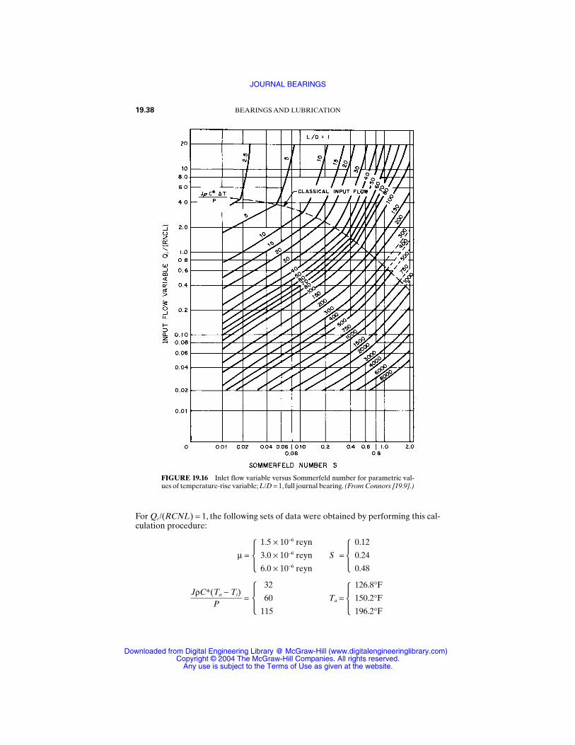
For Qi /(RCNL) = 1, the following sets of data were obtained by performing this cal-culation procedure:
1.5 × 10⁻⁶ reyn 0.12
µ = 3.0 × 10⁻⁶ reyn S = 0.24
6.0 × 10⁻⁶ reyn 0.48
32 126.8°F
JρC*(
PTa − Ti) = 60 Ta = 150.2°F
115 196.2°F
19.38 BEARINGS AND LUBRICATION
FIGURE 19.16 Inlet flow variable versus Sommerfeld number for parametric val-ues of temperature-rise variable; L/D = 1, full journal bearing. (From Connors [19.9].)
JOURNAL BEARINGS
Downloaded from Digital Engineering Library @ McGraw-Hill (www.digitalengineeringlibrary.com)Copyright © 2004 The McGraw-Hill Companies. All rights reserved.
Any use is subject to the Terms of Use as given at the website.
Using these and the lubricant µ versus T relation as presented in Table 19.16, wefind the operating point to be
Ta = 155°F µ = 3.2 × 10⁻⁶ reyn
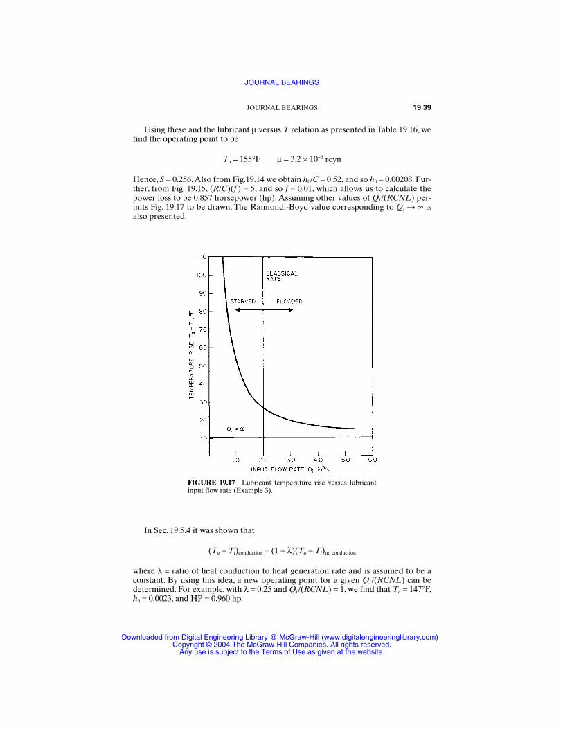
Hence, S = 0.256.Also from Fig.19.14 we obtain h0/C = 0.52, and so h0 = 0.00208. Fur-ther, from Fig. 19.15, (R/C)(f ) = 5, and so f = 0.01, which allows us to calculate thepower loss to be 0.857 horsepower (hp). Assuming other values of Qi /(RCNL) per-mits Fig. 19.17 to be drawn. The Raimondi-Boyd value corresponding to Qi → ∞ isalso presented.
JOURNAL BEARINGS 19.39
FIGURE 19.17 Lubricant temperature rise versus lubricantinput flow rate (Example 3).
In Sec. 19.5.4 it was shown that
(Ta − Ti)conduction = (1 − λ)(Ta − Ti)no conduction
where λ = ratio of heat conduction to heat generation rate and is assumed to be aconstant. By using this idea, a new operating point for a given Qi /(RCNL) can bedetermined. For example, with λ = 0.25 and Qi /(RCNL) = 1, we find that Ta = 147°F,h0 = 0.0023, and HP = 0.960 hp.
JOURNAL BEARINGS
Downloaded from Digital Engineering Library @ McGraw-Hill (www.digitalengineeringlibrary.com)Copyright © 2004 The McGraw-Hill Companies. All rights reserved.
Any use is subject to the Terms of Use as given at the website.
19.6.3 Optimization
In designing a journal bearing, a choice must be made among several potentialdesigns for the particular application. Thus the designer must establish an optimumdesign criterion for the bearing. The design criterion describes the designer’s objec-tive, and numerous criteria can be envisioned (e.g., minimizing frictional loss, mini-mizing the lubricant temperature rise, minimizing the lubricant supply to thebearing, and so forth).
The search for an optimum bearing design is best conducted with the aid of acomputer. However, optimum bearing design can also be achieved graphically. Moesand Bosma [19.10] developed a design chart for the full journal bearing whichenables the designer to select optimum bearing dimensions.This chart is constructedin terms of two dimensionless groups called X and Y here. The groups include twoquantities of primary importance to the bearing designer: minimum film thickness h0
and frictional torque Mj; the groups do not contain the bearing clearance. Thedimensionless groups are
X hR
0 2π
PNµ
1/2
Y WM
Rj
2πPNµ
1/2
(19.15)
Both X and Y can be written in terms of the Sommerfeld number. Recalling that h0 = C(1 − ε) and S = (µN/P)(R/C)2, we can easily show that
X = and Y = WM
Cj
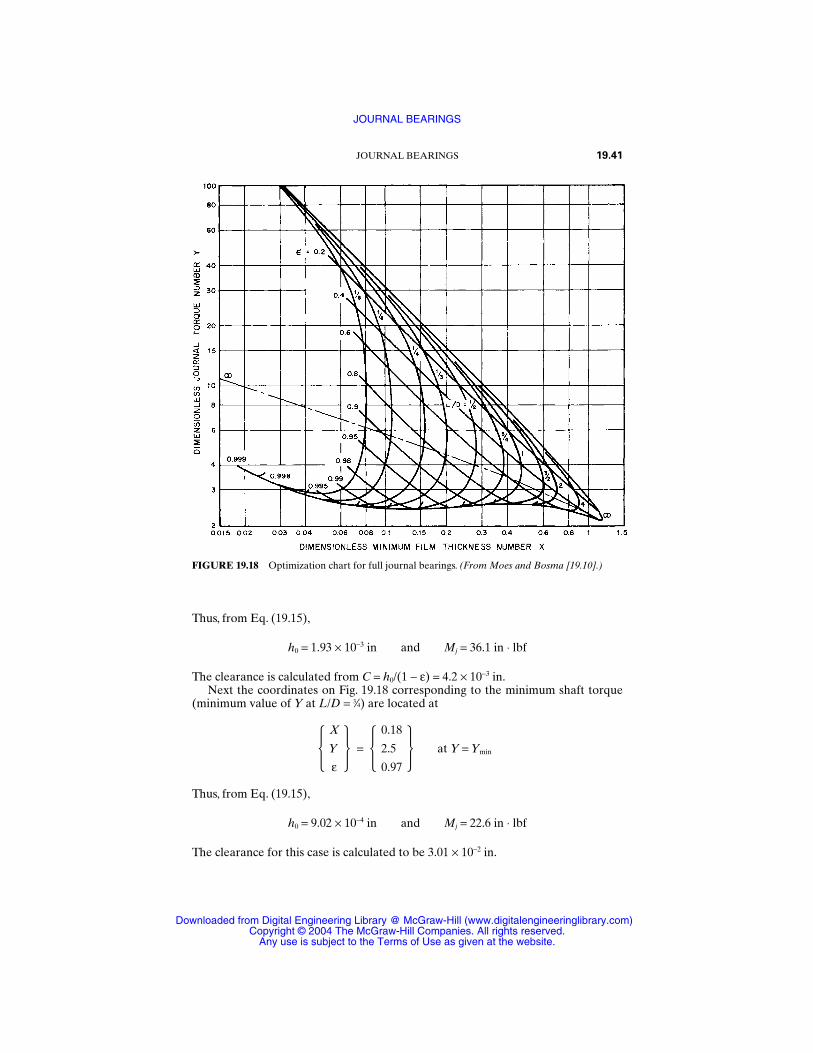
Figure 19.18 is a plot of full journal bearing design data on the XY plane. In thediagram, two families of curves can be distinguished: curves of constant L/D ratioand curves of constant ε. Use of this diagram permits rather complicated optimiza-tion procedures to be performed.
Example 4. Calculate the permissible range of minimum film thickness and bear-ing clearance that will produce minimum shaft torque for a full journal bearing oper-ating under the following conditions:
µ = 5 × 10⁻⁶ reyn D = 4 in
N = 1800 rev/min L = 3 in
W = 1800 lbf
Solution. As a first step, we calculate the largest h0 for the given conditions.Thisis easily accomplished by locating the coordinates on Fig. 19.18 corresponding to themaximum X for L/D = 3⁄4, or
X 0.385
Y = 4.0 at X = Xmax
ε 0.54
12πS
1 − ε2πS
19.40 BEARINGS AND LUBRICATION
JOURNAL BEARINGS
Downloaded from Digital Engineering Library @ McGraw-Hill (www.digitalengineeringlibrary.com)Copyright © 2004 The McGraw-Hill Companies. All rights reserved.
Any use is subject to the Terms of Use as given at the website.
Thus, from Eq. (19.15),
h0 = 1.93 × 10⁻³ in and Mj = 36.1 in ⋅ lbf
The clearance is calculated from C = h0/(1 − ε) = 4.2 × 10⁻³ in.Next the coordinates on Fig. 19.18 corresponding to the minimum shaft torque
(minimum value of Y at L/D = 3⁄4) are located at
X 0.18
Y = 2.5 at Y = Ymin
ε 0.97
Thus, from Eq. (19.15),
h0 = 9.02 × 10⁻⁴ in and Mj = 22.6 in ⋅ lbf
The clearance for this case is calculated to be 3.01 × 10⁻² in.
JOURNAL BEARINGS 19.41
FIGURE 19.18 Optimization chart for full journal bearings. (From Moes and Bosma [19.10].)
JOURNAL BEARINGS
Downloaded from Digital Engineering Library @ McGraw-Hill (www.digitalengineeringlibrary.com)Copyright © 2004 The McGraw-Hill Companies. All rights reserved.
Any use is subject to the Terms of Use as given at the website.
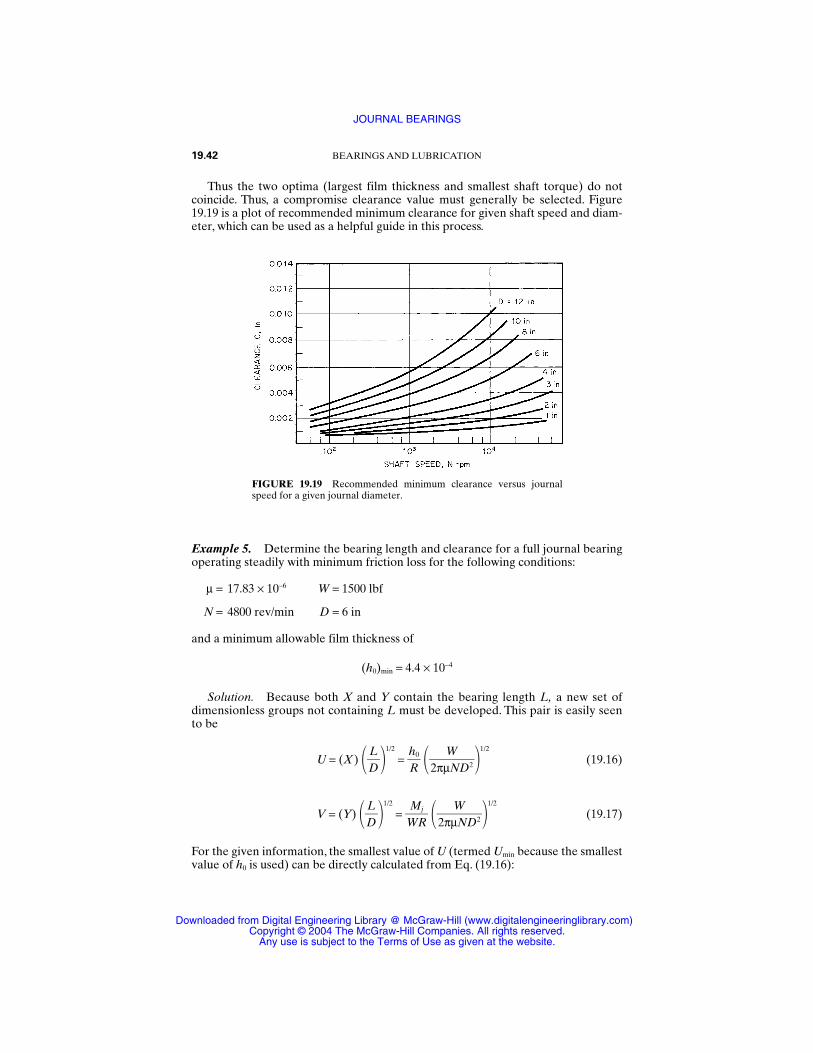
Thus the two optima (largest film thickness and smallest shaft torque) do notcoincide. Thus, a compromise clearance value must generally be selected. Figure19.19 is a plot of recommended minimum clearance for given shaft speed and diam-eter, which can be used as a helpful guide in this process.
19.42 BEARINGS AND LUBRICATION
FIGURE 19.19 Recommended minimum clearance versus journalspeed for a given journal diameter.
Example 5. Determine the bearing length and clearance for a full journal bearingoperating steadily with minimum friction loss for the following conditions:
µ = 17.83 × 10⁻⁶ W = 1500 lbf
N = 4800 rev/min D = 6 in
and a minimum allowable film thickness of
(h0)min = 4.4 × 10⁻⁴
Solution. Because both X and Y contain the bearing length L, a new set ofdimensionless groups not containing L must be developed. This pair is easily seento be
U = (X) DL
1/2
= hR
0 2πµ
WND2
1/2
(19.16)
V = (Y) DL
1/2
= WM
Rj
2πµWND2
1/2
(19.17)
For the given information, the smallest value of U (termed Umin because the smallestvalue of h0 is used) can be directly calculated from Eq. (19.16):
JOURNAL BEARINGS
Downloaded from Digital Engineering Library @ McGraw-Hill (www.digitalengineeringlibrary.com)Copyright © 2004 The McGraw-Hill Companies. All rights reserved.
Any use is subject to the Terms of Use as given at the website.
Umin = 0.10 Thus, X ≥ (0.10) DL
1/2
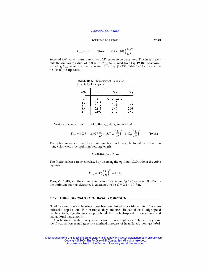
Selected L/D values permit an array of X values to be calculated. This in turn per-mits the minimum values of Y (that is, Ymin) to be read from Fig. 19.18. Then corre-sponding Vmin values can be calculated from Eq. (19.17). Table 19.17 contains theresults of this operation.
JOURNAL BEARINGS 19.43
TABLE 19.17 Summary of CalculatedResults for Example 5
Next a cubic equation is fitted to the Vmin data, and we find
Vmin = 4.057 − 11.927 DL
+ 18.742 DL
2
− 8.472 DL
3
(19.18)
The optimum value of L/D for a minimum friction loss can be found by differentia-tion, which yields the optimum bearing length:
L = 0.464D = 2.78 in
The frictional loss can be calculated by inserting the optimum L/D ratio in the cubicequation:
Vmin = (Y) DL
1/2
= 1.712
Thus, Y = 2.513, and the eccentricity ratio is read from Fig. 19.18 as ε 0.98. Finallythe optimum bearing clearance is calculated to be C 2.2 102 in.
19.7 GAS-LUBRICATED JOURNAL BEARINGS
Gas-lubricated journal bearings have been employed in a wide variety of modernindustrial applications. For example, they are used in dental drills, high-speedmachine tools, digital-computer peripheral devices, high-speed turbomachines, andnavigational instruments.
Gas bearings produce very little friction even at high speeds; hence, they havelow frictional losses and generate minimal amounts of heat. In addition, gas lubri-
JOURNAL BEARINGS
Downloaded from Digital Engineering Library @ McGraw-Hill (www.digitalengineeringlibrary.com)Copyright © 2004 The McGraw-Hill Companies. All rights reserved.
Any use is subject to the Terms of Use as given at the website.
cants are chemically very stable over a wide range of temperatures; they neitherfreeze nor boil; they are nonflammable; and they do not contaminate bearing sur-faces. Gas bearings also have low noise characteristics.
On the negative side, gas bearings do not have much load-carrying capacity andhave large startup wear. Also, because the gas film thickness is quite small, gas bear-ings require superior surface finish and manufacture. Great care must be exercisedwith the journal alignment. Further, thin films offer very little cushion or dampingcapacity; consequently, gas bearings are prone to certain vibrational instabilities.
19.7.1 Limiting Gas Bearing Solutions
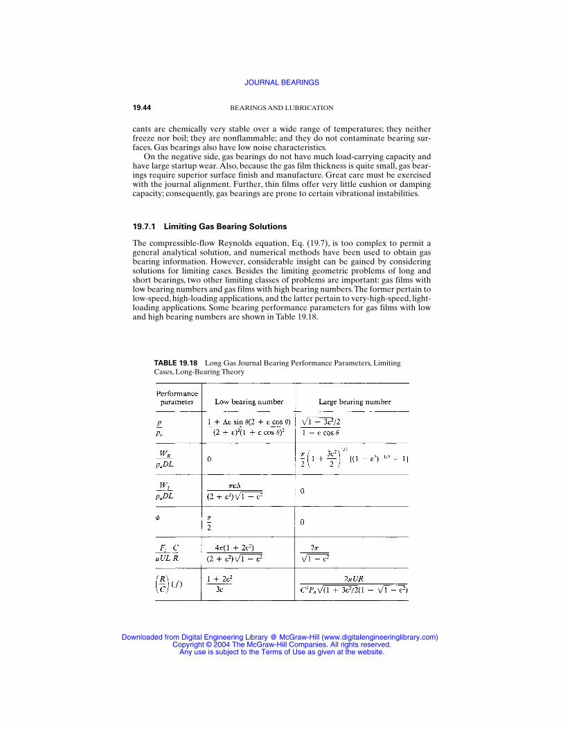
The compressible-flow Reynolds equation, Eq. (19.7), is too complex to permit ageneral analytical solution, and numerical methods have been used to obtain gasbearing information. However, considerable insight can be gained by consideringsolutions for limiting cases. Besides the limiting geometric problems of long andshort bearings, two other limiting classes of problems are important: gas films withlow bearing numbers and gas films with high bearing numbers.The former pertain tolow-speed, high-loading applications, and the latter pertain to very-high-speed, light-loading applications. Some bearing performance parameters for gas films with lowand high bearing numbers are shown in Table 19.18.
19.44 BEARINGS AND LUBRICATION
TABLE 19.18 Long Gas Journal Bearing Performance Parameters, LimitingCases, Long-Bearing Theory
JOURNAL BEARINGS
Downloaded from Digital Engineering Library @ McGraw-Hill (www.digitalengineeringlibrary.com)Copyright © 2004 The McGraw-Hill Companies. All rights reserved.
Any use is subject to the Terms of Use as given at the website.
19.7.2 Stability Considerations
The journal bearing of a rotating machine cannot be treated separately. It is part ofa complex dynamic system, and its design can influence the dynamic behavior of theentire system. Bearing damping controls vibration amplitude and tolerance to anyimbalance and, to a large extent, determines whether the rotor will be dynamicallystable. A bearing running in an unstable mode can lose its ability to support load,and rubbing contact can occur between the bearing and the shaft surfaces.
Rotor bearing instabilities are particularly troublesome in gas-lubricated bear-ings; the film is considerably thinner in gas bearings than in liquid-lubricated bear-ings and so does not possess the damping capacity.We can differentiate between twoforms of dynamic instability: synchronous whirl and half-frequency whirl (also calledfractional-frequency whirl and film whirl).
Synchronous Whirl. A rotating shaft experiences periodic deflection (forcedvibration) because of the distribution of load, the method of shaft support, thedegree of flexibility of the shaft, and any imbalance within the rotating mass. Thisdeflection causes the journal to orbit within its bearings at the rotational speed.When the frequency of this vibration occurs at the natural frequency (or criticalspeed) of the system, a resonance condition exists. In this condition, the amplitude ofvibration (size of the journal orbit) increases and can cause bearing failure. Becausethe shaft rotational speed and the critical speed coincide, this form of instability istermed synchronous whirl.
Since stable operation occurs on either side of the critical speed, the bearing sys-tem must be designed so that critical speeds do not exist in the operating speedrange. This can be accomplished by making the critical speeds either very large orvery small. Large critical speeds can be established by increasing the bearing stiff-ness by reducing the bearing clearance. Lower critical speeds can be established byincreasing the shaft flexibility. The instability can also be suppressed by mountingthe bearing in a flexible housing which introduces additional system damping.
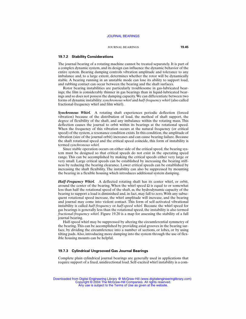
Half-Frequency Whirl. A deflected rotating shaft has its center whirl, or orbit,around the center of the bearing. When the whirl speed Ω is equal to or somewhatless than half the rotational speed of the shaft, ω, the hydrodynamic capacity of thebearing to support a load is diminished and, in fact, may fall to zero.With any subse-quent rotational speed increase, the whirl amplitude will increase, and the bearingand journal may come into violent contact. This form of self-activated vibrationalinstability is called half-frequency or half-speed whirl. Because the whirl speed forgas bearings is generally less than the rotational speed, the instability is also termedfractional-frequency whirl. Figure 19.20 is a map for assessing the stability of a fulljournal bearing.
Half-speed whirl may be suppressed by altering the circumferential symmetry ofthe bearing. This can be accomplished by providing axial grooves in the bearing sur-face, by dividing the circumference into a number of sections, or lobes, or by usingtilting pads.Also, introducing more damping into the system through the use of flex-ible housing mounts can be helpful.
19.7.3 Cylindrical Ungrooved Gas Journal Bearings
Complete plain cylindrical journal bearings are generally used in applications thatrequire support of a fixed, unidirectional load. Self-excited whirl instability is a com-
JOURNAL BEARINGS 19.45
JOURNAL BEARINGS
Downloaded from Digital Engineering Library @ McGraw-Hill (www.digitalengineeringlibrary.com)Copyright © 2004 The McGraw-Hill Companies. All rights reserved.
Any use is subject to the Terms of Use as given at the website.
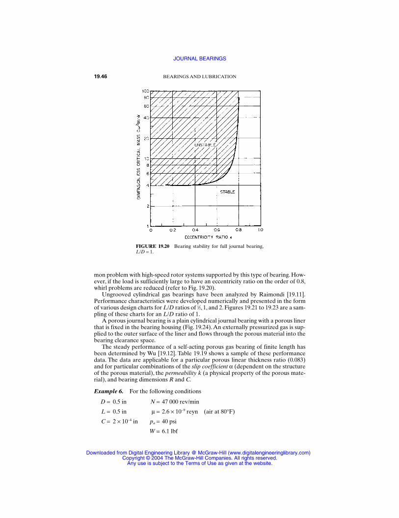
mon problem with high-speed rotor systems supported by this type of bearing. How-ever, if the load is sufficiently large to have an eccentricity ratio on the order of 0.8,whirl problems are reduced (refer to Fig. 19.20).
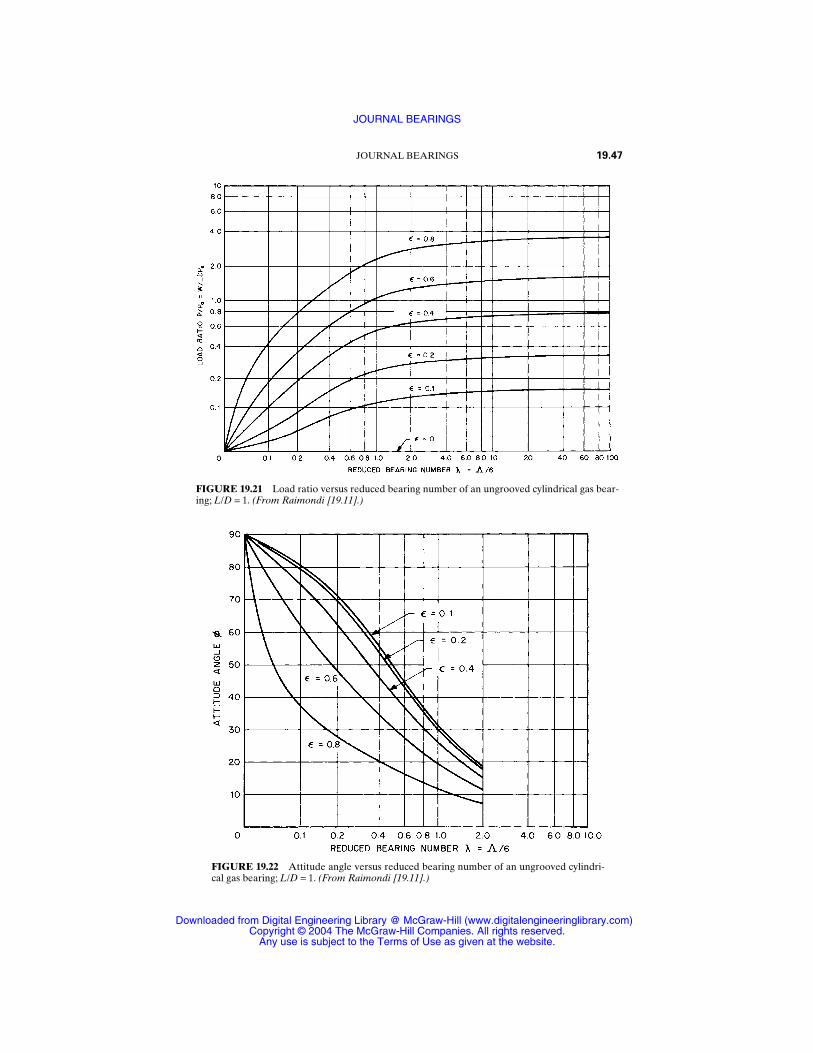
Ungrooved cylindrical gas bearings have been analyzed by Raimondi [19.11].Performance characteristics were developed numerically and presented in the formof various design charts for L/D ratios of 1⁄2, 1, and 2. Figures 19.21 to 19.23 are a sam-pling of these charts for an L/D ratio of 1.
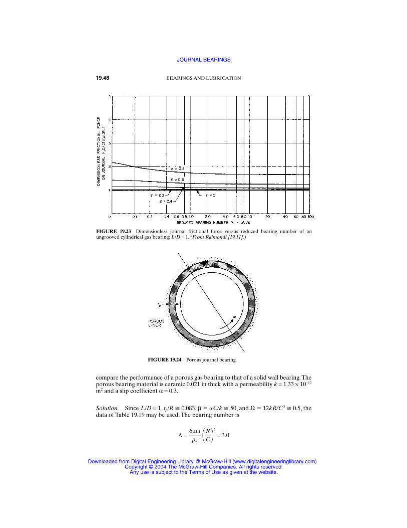
A porous journal bearing is a plain cylindrical journal bearing with a porous linerthat is fixed in the bearing housing (Fig. 19.24). An externally pressurized gas is sup-plied to the outer surface of the liner and flows through the porous material into thebearing clearance space.
The steady performance of a self-acting porous gas bearing of finite length hasbeen determined by Wu [19.12]. Table 19.19 shows a sample of these performancedata. The data are applicable for a particular porous linear thickness ratio (0.083)and for particular combinations of the slip coefficient α (dependent on the structureof the porous material), the permeability k (a physical property of the porous mate-rial), and bearing dimensions R and C.
Example 6. For the following conditions
D = 0.5 in N = 47 000 rev/min
L = 0.5 in µ = 2.6 × 10⁻⁹ reyn (air at 80°F)
C = 2 × 10⁻⁴ in pa = 40 psi
W = 6.1 lbf
19.46 BEARINGS AND LUBRICATION
FIGURE 19.20 Bearing stability for full journal bearing,L/D = 1.
JOURNAL BEARINGS
Downloaded from Digital Engineering Library @ McGraw-Hill (www.digitalengineeringlibrary.com)Copyright © 2004 The McGraw-Hill Companies. All rights reserved.
Any use is subject to the Terms of Use as given at the website.
JOURNAL BEARINGS 19.47
FIGURE 19.21 Load ratio versus reduced bearing number of an ungrooved cylindrical gas bear-ing; L/D = 1. (From Raimondi [19.11].)
FIGURE 19.22 Attitude angle versus reduced bearing number of an ungrooved cylindri-cal gas bearing; L/D = 1. (From Raimondi [19.11].)
JOURNAL BEARINGS
Downloaded from Digital Engineering Library @ McGraw-Hill (www.digitalengineeringlibrary.com)Copyright © 2004 The McGraw-Hill Companies. All rights reserved.
Any use is subject to the Terms of Use as given at the website.
compare the performance of a porous gas bearing to that of a solid wall bearing.Theporous bearing material is ceramic 0.021 in thick with a permeability k = 1.33 × 10⁻¹²
in2 and a slip coefficient α = 0.3.
Solution. Since L/D = 1, tp/R 0.083, C/k 50, and 12kR/C 3 0.5, thedata of Table 19.19 may be used. The bearing number is
Λ = 6pµ
a
ω
RC
2
= 3.0
19.48 BEARINGS AND LUBRICATION
FIGURE 19.23 Dimensionless journal frictional force versus reduced bearing number of anungrooved cylindrical gas bearing; L/D = 1. (From Raimondi [19.11].)
FIGURE 19.24 Porous journal bearing.
JOURNAL BEARINGS
Downloaded from Digital Engineering Library @ McGraw-Hill (www.digitalengineeringlibrary.com)Copyright © 2004 The McGraw-Hill Companies. All rights reserved.
Any use is subject to the Terms of Use as given at the website.
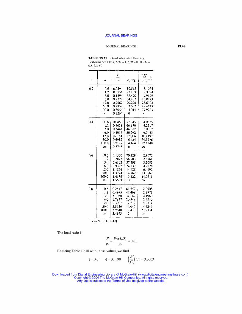
The load ratio is
pP
a = = 0.61
Entering Table 19.18 with these values, we find
ε = 0.6 φ = 37.598 RC
(f ) = 3.3003
W/(LD)
pa
JOURNAL BEARINGS 19.49
TABLE 19.19 Gas-Lubricated Bearing Performance Data, L/D = 1, tp/R = 0.083, Ω =0.5, β = 50
JOURNAL BEARINGS
Downloaded from Digital Engineering Library @ McGraw-Hill (www.digitalengineeringlibrary.com)Copyright © 2004 The McGraw-Hill Companies. All rights reserved.
Any use is subject to the Terms of Use as given at the website.
For the same values we can find from Figs. 19.21 to 19.23 for the solid wall bearing ε = 0.54, φ = 33.7°, and
2πµ
FUjC
RL = 1.18
From the last value, we may compute for comparative purposes
RC
(f ) = 3.038
Thus the porous bearing operates at a larger eccentricity ratio (which indicates bet-ter stability) but has larger frictional loss. On the other hand, for a given ε, theporous bearing has a lower load capacity compared to the solid wall bearing. Thisloss of load capacity becomes more severe as the eccentricity ratio is increased.
19.7.4 Axially Grooved Gas Journal Bearings
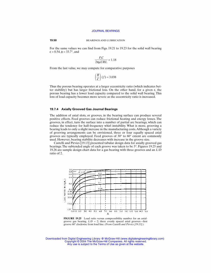
The addition of axial slots, or grooves, in the bearing surface can produce severalpositive effects. Feed grooves can reduce frictional heating and energy losses. Thegrooves, in effect, turn the surface into a number of partial arc bearings, which canreduce the tendency for half-frequency whirl instability. What is more, grooving abearing leads to only a slight increase in the manufacturing costs.Although a varietyof grooving arrangements can be envisioned, three or four equally spaced axialgrooves are typically employed. Feed grooves of 30° to 60° extent are commonlyused. However, bearing stability decreases with increase in the groove size.
Castelli and Pirvics [19.13] presented tabular design data for axially grooved gasbearings. The subtended angle of each groove was taken to be 5°. Figures 19.25 and19.26 are sample design chart data for a gas bearing with three grooves and an L/Dratio of 2.
19.50 BEARINGS AND LUBRICATION
FIGURE 19.25 Load ratio versus compressibility number for an axial-groove gas bearing, L/D = 2; three evenly spaced axial grooves—firstgroove 60° clockwise from load line. (From Castelli and Pirvics [19.13].)
JOURNAL BEARINGS
Downloaded from Digital Engineering Library @ McGraw-Hill (www.digitalengineeringlibrary.com)Copyright © 2004 The McGraw-Hill Companies. All rights reserved.
Any use is subject to the Terms of Use as given at the website.
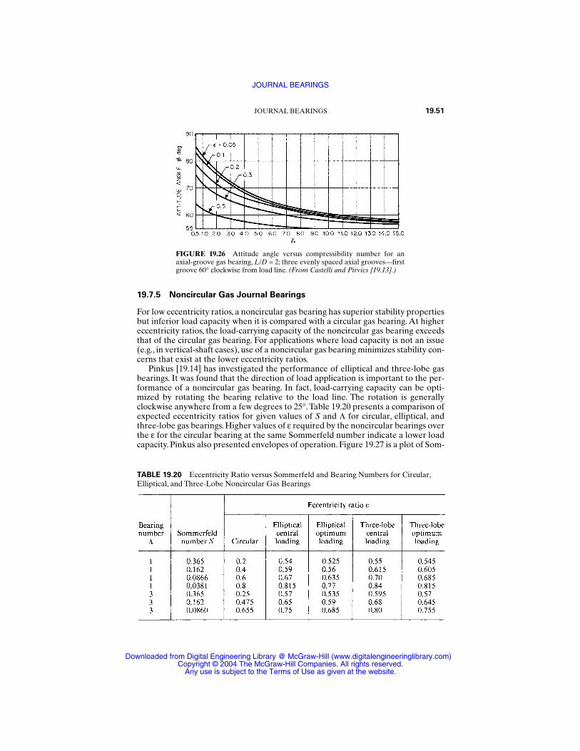
19.7.5 Noncircular Gas Journal Bearings
For low eccentricity ratios, a noncircular gas bearing has superior stability propertiesbut inferior load capacity when it is compared with a circular gas bearing. At highereccentricity ratios, the load-carrying capacity of the noncircular gas bearing exceedsthat of the circular gas bearing. For applications where load capacity is not an issue(e.g., in vertical-shaft cases), use of a noncircular gas bearing minimizes stability con-cerns that exist at the lower eccentricity ratios.
Pinkus [19.14] has investigated the performance of elliptical and three-lobe gasbearings. It was found that the direction of load application is important to the per-formance of a noncircular gas bearing. In fact, load-carrying capacity can be opti-mized by rotating the bearing relative to the load line. The rotation is generallyclockwise anywhere from a few degrees to 25°.Table 19.20 presents a comparison ofexpected eccentricity ratios for given values of S and Λ for circular, elliptical, andthree-lobe gas bearings. Higher values of ε required by the noncircular bearings overthe ε for the circular bearing at the same Sommerfeld number indicate a lower loadcapacity. Pinkus also presented envelopes of operation. Figure 19.27 is a plot of Som-
JOURNAL BEARINGS 19.51
FIGURE 19.26 Attitude angle versus compressibility number for anaxial-groove gas bearing, L/D = 2; three evenly spaced axial grooves—firstgroove 60° clockwise from load line. (From Castelli and Pirvics [19.13].)
TABLE 19.20 Eccentricity Ratio versus Sommerfeld and Bearing Numbers for Circular,Elliptical, and Three-Lobe Noncircular Gas Bearings
JOURNAL BEARINGS
Downloaded from Digital Engineering Library @ McGraw-Hill (www.digitalengineeringlibrary.com)Copyright © 2004 The McGraw-Hill Companies. All rights reserved.
Any use is subject to the Terms of Use as given at the website.
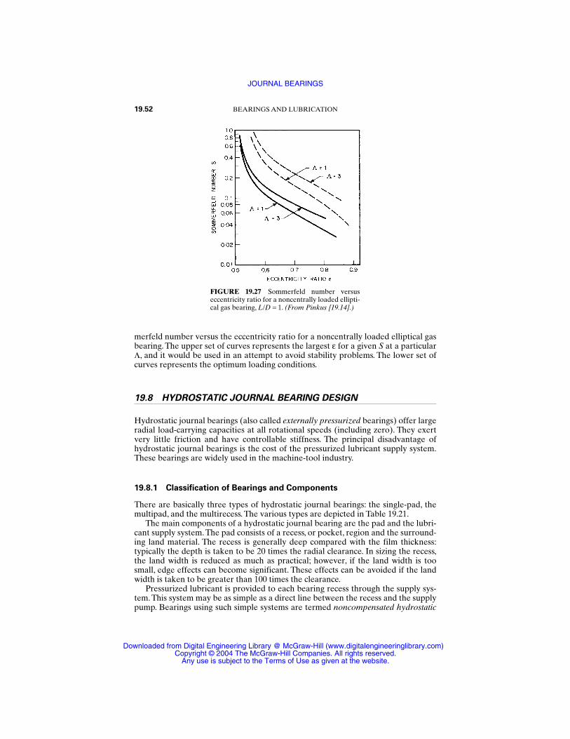
merfeld number versus the eccentricity ratio for a noncentrally loaded elliptical gasbearing. The upper set of curves represents the largest ε for a given S at a particularΛ, and it would be used in an attempt to avoid stability problems. The lower set ofcurves represents the optimum loading conditions.
19.8 HYDROSTATIC JOURNAL BEARING DESIGN
Hydrostatic journal bearings (also called externally pressurized bearings) offer largeradial load-carrying capacities at all rotational speeds (including zero). They exertvery little friction and have controllable stiffness. The principal disadvantage ofhydrostatic journal bearings is the cost of the pressurized lubricant supply system.These bearings are widely used in the machine-tool industry.
19.8.1 Classification of Bearings and Components
There are basically three types of hydrostatic journal bearings: the single-pad, themultipad, and the multirecess. The various types are depicted in Table 19.21.
The main components of a hydrostatic journal bearing are the pad and the lubri-cant supply system. The pad consists of a recess, or pocket, region and the surround-ing land material. The recess is generally deep compared with the film thickness:typically the depth is taken to be 20 times the radial clearance. In sizing the recess,the land width is reduced as much as practical; however, if the land width is toosmall, edge effects can become significant. These effects can be avoided if the landwidth is taken to be greater than 100 times the clearance.
Pressurized lubricant is provided to each bearing recess through the supply sys-tem. This system may be as simple as a direct line between the recess and the supplypump. Bearings using such simple systems are termed noncompensated hydrostatic
19.52 BEARINGS AND LUBRICATION
FIGURE 19.27 Sommerfeld number versuseccentricity ratio for a noncentrally loaded ellipti-cal gas bearing, L/D = 1. (From Pinkus [19.14].)
JOURNAL BEARINGS
Downloaded from Digital Engineering Library @ McGraw-Hill (www.digitalengineeringlibrary.com)Copyright © 2004 The McGraw-Hill Companies. All rights reserved.
Any use is subject to the Terms of Use as given at the website.
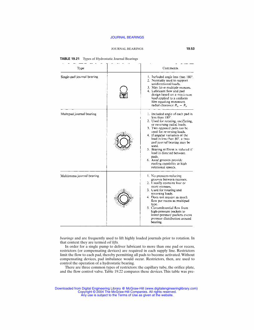
bearings and are frequently used to lift highly loaded journals prior to rotation. Inthat context they are termed oil lifts.
In order for a single pump to deliver lubricant to more than one pad or recess,restrictors (or compensating devices) are required in each supply line. Restrictorslimit the flow to each pad, thereby permitting all pads to become activated. Withoutcompensating devices, pad imbalance would occur. Restrictors, then, are used tocontrol the operation of a hydrostatic bearing.
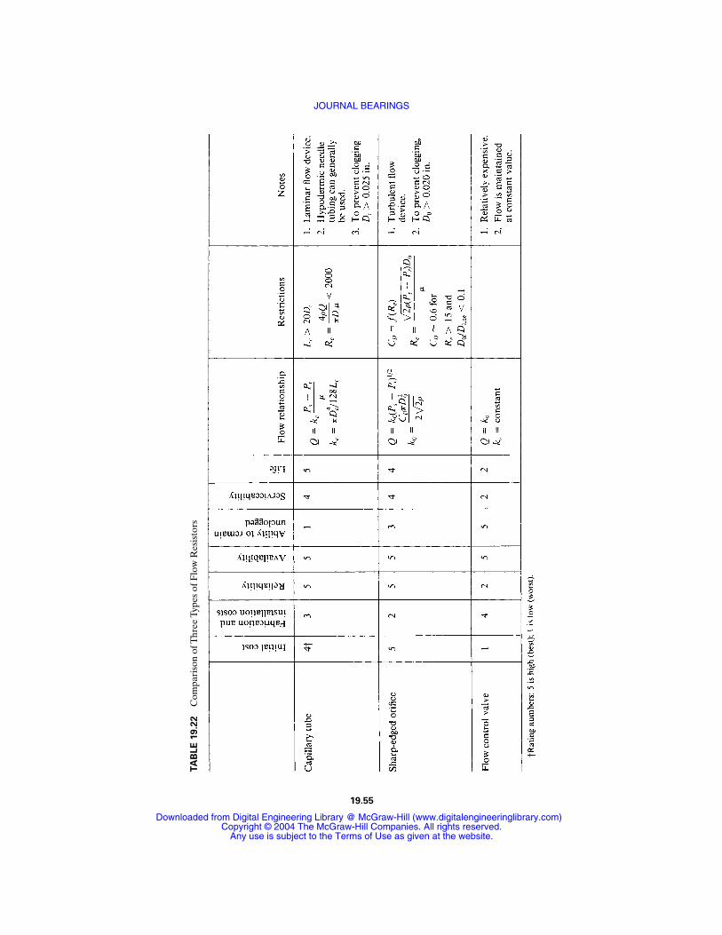
There are three common types of restrictors: the capillary tube, the orifice plate,and the flow control valve. Table 19.22 compares these devices. This table was pre-
JOURNAL BEARINGS 19.53
TABLE 19.21 Types of Hydrostatic Journal Bearings
JOURNAL BEARINGS
Downloaded from Digital Engineering Library @ McGraw-Hill (www.digitalengineeringlibrary.com)Copyright © 2004 The McGraw-Hill Companies. All rights reserved.
Any use is subject to the Terms of Use as given at the website.
pared from a comprehensive series of papers on hydrostatic bearing design by Rip-pel [19.15]. In addition to flow-load control, the resistor affects the stiffness of thebearing. Bearing stiffness is related to the ability of the bearing to tolerate anychanges in the applied load.
19.8.2 Design Parameters
For hydrostatic journal bearings at low rotational speeds, the primary design param-eters are maximum load, lubricant flow rate, and stiffness. Of secondary importanceare considerations of frictional horsepower and lubricant temperature rise.
The load-carrying capacity of a hydrostatic journal bearing is generally written as
W = afAppr (19.19)
where af = pad load coefficient, Ap = projected bearing area, and pr = recess pressure.The pad load coefficient is dimensionless and physically represents the ratio of theaverage lubricant pressure in the pad to the lubricant pressure supplied to the pad.O’Donoghue and Rowe [19.16] give equations for af for both multirecess and multi-pad bearings.
The lubricant flow rate may be determined from
Q = qf h
µ
3pr (19.20)
where qf = flow factor for a single pad.The flow factor depends on the geometry andland widths of the bearing.
Journal bearing stiffness expresses the ability of the bearing to accommodate anychanges in the applied load. Stiffness is proportional to the slope of the bearing loadversus film thickness curve, or
s = − d
d
W
h (19.21)
Stiffness will depend on the method of flow control (capillary tube, etc.) and theamount of circumferential flow. O’Donoghue and Rowe [19.16] provide a detailedderivation of the journal bearing stiffness and have developed equations for bothmultipad and multirecess bearings.
19.8.3 Design Procedures
A variety of design procedures are available for hydrostatic bearings. Some arebased on experimental findings, whereas others are based on numerical solutions ofthe Reynolds equation.
Many existing methods incorporate numerous charts and tables which clearlyplace a limit on the methods; in order to use these procedures, the appropriate ref-erence must be consulted.Alternatively, O’Donoghue and Rowe [19.16] have devel-oped a general approximate method of design that does not require the use ofvarious design charts.The method is strictly valid for thin land bearings, and many ofthe parameters are conservatively estimated. The following is a condensation of thisdesign procedure for a multirecess bearing:
19.54 BEARINGS AND LUBRICATION
JOURNAL BEARINGS
Downloaded from Digital Engineering Library @ McGraw-Hill (www.digitalengineeringlibrary.com)Copyright © 2004 The McGraw-Hill Companies. All rights reserved.
Any use is subject to the Terms of Use as given at the website.
TA
BLE
19.2
2C
ompa
riso
n of
Thr
ee T
ypes
of F
low
Res
isto
rs
19.55
JOURNAL BEARINGS
Downloaded from Digital Engineering Library @ McGraw-Hill (www.digitalengineeringlibrary.com)Copyright © 2004 The McGraw-Hill Companies. All rights reserved.
Any use is subject to the Terms of Use as given at the website.

Design Specification
1. Set the maximum load W.
2. Select the number of recesses n (typically n = 4, but n = 6 for high-precisionbearings).
3. Select a pressure ratio pr /ps (a design value of 0.5 is recommended).
Bearing Dimensions
1. Calculate the bearing diameter D = W/50 in.2. Set width L = D.
3. Calculate the axial-flow land width a (refer to Fig. 19.28; recommended value:a = L/4).
19.56 BEARINGS AND LUBRICATION
FIGURE 19.28 Hydrostatic pad geometry.
4. Calculate the circumferential land width b [refer to Fig. 19.28; recommendedvalue: b = πD/(4n)].
5. Calculate the projected pad area Ap = D(L − a).6. Calculate the recess area for one pad only: Ar = (πD − nb)(L − a)/n.
7. Calculate the effective frictional area: Af = (πDL/n) − 0.75Af.
Miscellaneous Coefficients and Parameters
1. Establish a design value of film thickness hd (recommended value: 50 to 10 timeslarger than the machinery tolerance on h).
2. Calculate the circumferential flow factor γ = na(L − a)/(πDb); for recommendedvalues of D, L, a, and b: γ = 3⁄4(n/π)2.
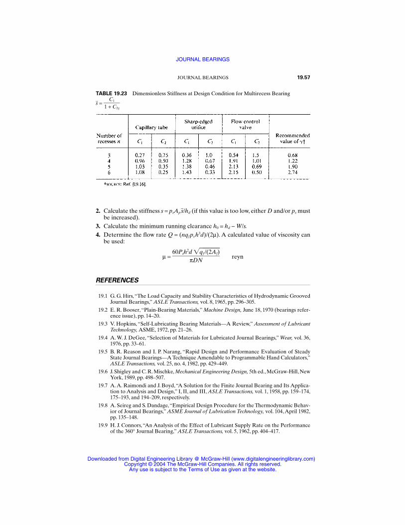
3. Compute the design dimensionless stiffness parameter s from Table 19.23depending on the method of flow control selected.
4. Calculate the flow factor qf = πD/(6an).
Performance Parameters
1. Calculate the minimum supply pressure ps,min = 2W/(afAp) [recommended: af = s(capillary tube at design Table 19.23)].
JOURNAL BEARINGS
Downloaded from Digital Engineering Library @ McGraw-Hill (www.digitalengineeringlibrary.com)Copyright © 2004 The McGraw-Hill Companies. All rights reserved.
Any use is subject to the Terms of Use as given at the website.
2. Calculate the stiffness s = psAps/hd (if this value is too low, either D and/or ps mustbe increased).
3. Calculate the minimum running clearance h0 = hd − W/s.4. Determine the flow rate Q = (nqfpsh3d)/(2µ). A calculated value of viscosity can
be used:
µ = reyn
REFERENCES
19.1 G. G. Hirs, “The Load Capacity and Stability Characteristics of Hydrodynamic GroovedJournal Bearings,” ASLE Transactions, vol. 8, 1965, pp. 296–305.
19.2 E. R. Booser, “Plain-Bearing Materials,” Machine Design, June 18, 1970 (bearings refer-ence issue), pp. 14–20.
19.3 V. Hopkins, “Self-Lubricating Bearing Materials—A Review,” Assessment of LubricantTechnology, ASME, 1972, pp. 21–26.
19.4 A. W. J. DeGee, “Selection of Materials for Lubricated Journal Bearings,” Wear, vol. 36,1976, pp. 33–61.
19.5 B. R. Reason and I. P. Narang, “Rapid Design and Performance Evaluation of SteadyState Journal Bearings—A Technique Amendable to Programmable Hand Calculators,”ASLE Transactions, vol. 25, no. 4, 1982, pp. 429–449.
19.6 J. Shigley and C. R. Mischke, Mechanical Engineering Design, 5th ed., McGraw-Hill, NewYork, 1989, pp. 498–507.
19.7 A. A. Raimondi and J. Boyd, “A Solution for the Finite Journal Bearing and Its Applica-tion to Analysis and Design,” I, II, and III, ASLE Transactions, vol. 1, 1958, pp. 159–174,175–193, and 194–209, respectively.
19.8 A. Seireg and S. Dandage,“Empirical Design Procedure for the Thermodynamic Behav-ior of Journal Bearings,” ASME Journal of Lubrication Technology, vol. 104, April 1982,pp. 135–148.
19.9 H. J. Connors, “An Analysis of the Effect of Lubricant Supply Rate on the Performanceof the 360° Journal Bearing,” ASLE Transactions, vol. 5, 1962, pp. 404–417.
60Psh2d qf /(2Af)
πDN
JOURNAL BEARINGS 19.57
TABLE 19.23 Dimensionless Stiffness at Design Condition for Multirecess Bearing
s =C1
1 + C2γ
JOURNAL BEARINGS
Downloaded from Digital Engineering Library @ McGraw-Hill (www.digitalengineeringlibrary.com)Copyright © 2004 The McGraw-Hill Companies. All rights reserved.
Any use is subject to the Terms of Use as given at the website.
19.10 H. Moes and R. Bosma, “Design Charts for Optimum Bearing Configurations: 1—TheFull Journal Bearing,” ASME Journal of Lubrication Technology, vol. 93, April 1971, pp.302–306.
19.11 A. A. Raimondi, “A Numerical Solution for the Gas Lubricated Full Journal Bearing ofFinite Length,” ASLE Transactions, vol. 4, 1961, pp. 131–155.
19.12 E. R. Wu, “Gas-Lubricated Porous Bearings of Finite Length—Self-Acting JournalBearings,” ASME Journal of Lubrication Technology, vol. 101, July 1979, pp. 338–348.
19.13 V. Castelli and J. Pirvics,“Equilibrium Characteristics of Axial-Grooved Gas-LubricatedBearings,” ASME Journal of Lubrication Technology, vol. 89, April 1967, pp. 177–196.
19.14 O. Pinkus, “Analysis of Noncircular Gas Journal Bearings,” ASME Journal of Lubrica-tion Technology, vol. 87, October 1975, pp. 616–619.
19.15 H. C. Rippel, “Design of Hydrostatic Bearings,” Machine Design, parts 1 to 10, Aug. 1 toDec. 5, 1963.
19.16 J. P. O’Donoghue and W. B. Rowe, “Hydrostatic Bearing Design,” Tribology, vol. 2,February 1969, pp. 25–71.
19.58 BEARINGS AND LUBRICATION
JOURNAL BEARINGS
Downloaded from Digital Engineering Library @ McGraw-Hill (www.digitalengineeringlibrary.com)Copyright © 2004 The McGraw-Hill Companies. All rights reserved.
Any use is subject to the Terms of Use as given at the website.
CHAPTER 20LUBRICATION
A. R. Lansdown, M.Sc., Ph.D.Director, Swansea Tribology Centre
University College of SwanseaSwansea, United Kingdom
20.1 FUNCTIONS AND TYPES OF LUBRICANT / 20.1
20.2 SELECTION OF LUBRICANT TYPE / 20.2
20.3 LIQUID LUBRICANTS: PRINCIPLES AND REQUIREMENTS / 20.3
20.4 LUBRICANT VISCOSITY / 20.6
20.5 BOUNDARY LUBRICATION / 20.9
20.6 DETERIORATION PROBLEMS / 20.12
20.7 SELECTING THE OIL TYPE / 20.14
20.8 LUBRICATING GREASES / 20.17
20.9 SOLID LUBRICANTS / 20.22
20.10 GAS LUBRICATION / 20.26
20.11 LUBRICANT FEED SYSTEMS / 20.26
20.12 LUBRICANT STORAGE / 20.29
REFERENCES / 20.30
20.1 FUNCTIONS AND TYPES OF LUBRICANT
Whenever relative movement takes place between two surfaces in contact, there willbe resistance to movement. This resistance is called the frictional force, or simplyfriction. Where this situation exists, it is often desirable to reduce, control, or modifythe friction.
Broadly speaking, any process by which the friction in a moving contact isreduced may be described as lubrication. Traditionally this description has presentedno problems. Friction reduction was obtained by introducing a solid or liquid mate-rial, called a lubricant, into the contact, so that the surfaces in relative motion wereseparated by a film of the lubricant. Lubricants consisted of a relatively few types ofmaterial, such as natural or mineral oils, graphite, molybdenum disulfide, and talc,and the relationship between lubricants and the process of lubrication was clear andunambiguous.
Recent technological developments have confused this previously clear picture.Friction reduction may now be provided by liquids, solids, or gases or by physical orchemical modification of the surfaces themselves. Alternatively, the sliding compo-nents may be manufactured from a material which is itself designed to reduce fric-tion or within which a lubricant has been uniformly or nonuniformly dispersed. Suchsystems are sometimes described as “unlubricated,” but this is clearly a matter of ter-minology. The system may be unconventionally lubricated, but it is certainly notunlubricated.
20.1
Source: STANDARD HANDBOOK OF MACHINE DESIGN
Downloaded from Digital Engineering Library @ McGraw-Hill (www.digitalengineeringlibrary.com)Copyright © 2004 The McGraw-Hill Companies. All rights reserved.
Any use is subject to the Terms of Use as given at the website.
On the other hand, lubrication may be used to modify friction but not specificallyto reduce it. Certain composite brake materials may incorporate graphite or molyb-denum disulfide, whose presence is designed to ensure steady or consistent levels offriction. The additives are clearly lubricants, and it would be pedantic to assert thattheir use in brake materials is not lubrication.
This introduction is intended only to generate an open-minded approach to theprocesses of lubrication and to the selection of lubricants. In practice, the vast major-ity of systems are still lubricated by conventional oils or greases or by equallyancient but less conventional solid lubricants. It is when some aspect of the systemmakes the use of these simple lubricants difficult or unsatisfactory that the widerinterpretation of lubrication may offer solutions. In addition to their primary func-tion of reducing or controlling friction, lubricants are usually expected to reducewear and perhaps also to reduce heat or corrosion.
In terms of volume, the most important types of lubricant are still the liquids(oils) and semiliquids (greases). Solid lubricants have been rapidly increasing inimportance since about 1950, especially for environmental conditions which are toosevere for oils and greases. Gases can be used as lubricants in much the same way asliquids, but as is explained later, the low viscosities of gases increase the difficultiesof bearing design and construction.
20.2 SELECTION OF LUBRICANT TYPE
A useful first principle in selecting a type of lubrication is to choose the simplesttechnique which will work satisfactorily. In very many cases this will mean insertinga small quantity of oil or grease in the component on initial assembly; this is almostnever replaced or refilled. Typical examples are door locks, hinges, car-windowwinders, switches, clocks, and watches.
This simple system is likely to be unsatisfactory if the loads or speeds are high orif the service life is long and continuous. Then it becomes necessary to choose thelubricant with care and often to use a replenishment system.
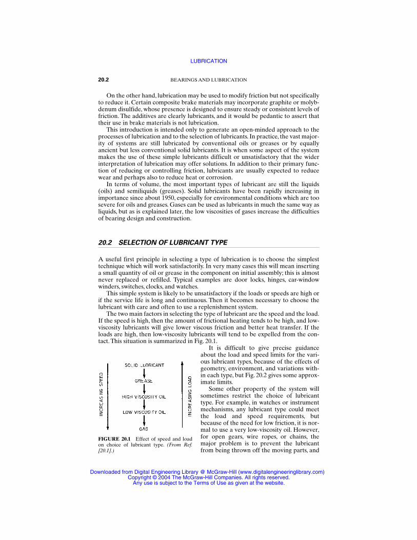
The two main factors in selecting the type of lubricant are the speed and the load.If the speed is high, then the amount of frictional heating tends to be high, and low-viscosity lubricants will give lower viscous friction and better heat transfer. If theloads are high, then low-viscosity lubricants will tend to be expelled from the con-tact. This situation is summarized in Fig. 20.1.
It is difficult to give precise guidanceabout the load and speed limits for the vari-ous lubricant types, because of the effects ofgeometry, environment, and variations with-in each type, but Fig. 20.2 gives some approx-imate limits.
Some other property of the system willsometimes restrict the choice of lubricanttype. For example, in watches or instrumentmechanisms, any lubricant type could meetthe load and speed requirements, butbecause of the need for low friction, it is nor-mal to use a very low-viscosity oil. However,for open gears, wire ropes, or chains, themajor problem is to prevent the lubricantfrom being thrown off the moving parts, and
20.2 BEARINGS AND LUBRICATION
FIGURE 20.1 Effect of speed and loadon choice of lubricant type. (From Ref.[20.1].)
LUBRICATION
Downloaded from Digital Engineering Library @ McGraw-Hill (www.digitalengineeringlibrary.com)Copyright © 2004 The McGraw-Hill Companies. All rights reserved.
Any use is subject to the Terms of Use as given at the website.
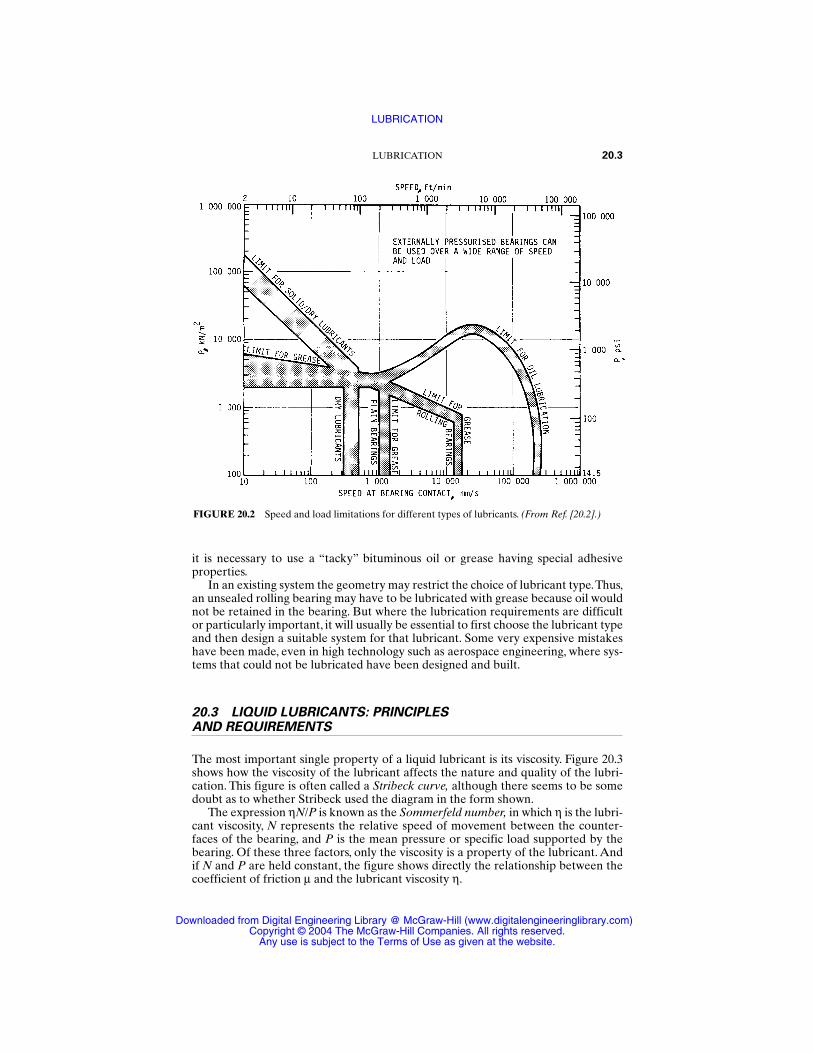
it is necessary to use a “tacky” bituminous oil or grease having special adhesiveproperties.
In an existing system the geometry may restrict the choice of lubricant type.Thus,an unsealed rolling bearing may have to be lubricated with grease because oil wouldnot be retained in the bearing. But where the lubrication requirements are difficultor particularly important, it will usually be essential to first choose the lubricant typeand then design a suitable system for that lubricant. Some very expensive mistakeshave been made, even in high technology such as aerospace engineering, where sys-tems that could not be lubricated have been designed and built.
20.3 LIQUID LUBRICANTS: PRINCIPLES AND REQUIREMENTS
The most important single property of a liquid lubricant is its viscosity. Figure 20.3shows how the viscosity of the lubricant affects the nature and quality of the lubri-cation. This figure is often called a Stribeck curve, although there seems to be somedoubt as to whether Stribeck used the diagram in the form shown.
The expression ηN/P is known as the Sommerfeld number, in which η is the lubri-cant viscosity, N represents the relative speed of movement between the counter-faces of the bearing, and P is the mean pressure or specific load supported by thebearing. Of these three factors, only the viscosity is a property of the lubricant. Andif N and P are held constant, the figure shows directly the relationship between thecoefficient of friction µ and the lubricant viscosity η.
LUBRICATION 20.3
FIGURE 20.2 Speed and load limitations for different types of lubricants. (From Ref. [20.2].)
LUBRICATION
Downloaded from Digital Engineering Library @ McGraw-Hill (www.digitalengineeringlibrary.com)Copyright © 2004 The McGraw-Hill Companies. All rights reserved.
Any use is subject to the Terms of Use as given at the website.
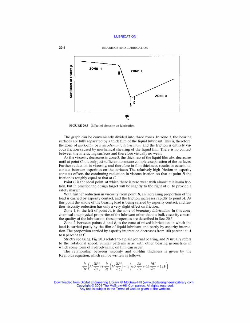
The graph can be conveniently divided into three zones. In zone 3, the bearingsurfaces are fully separated by a thick film of the liquid lubricant. This is, therefore,the zone of thick-film or hydrodynamic lubrication, and the friction is entirely vis-cous friction caused by mechanical shearing of the liquid film. There is no contactbetween the interacting surfaces and therefore virtually no wear.
As the viscosity decreases in zone 3, the thickness of the liquid film also decreasesuntil at point C it is only just sufficient to ensure complete separation of the surfaces.Further reduction in viscosity, and therefore in film thickness, results in occasionalcontact between asperities on the surfaces. The relatively high friction in asperitycontacts offsets the continuing reduction in viscous friction, so that at point B thefriction is roughly equal to that at C.
Point C is the ideal point, at which there is zero wear with almost minimum fric-tion, but in practice the design target will be slightly to the right of C, to provide asafety margin.
With further reduction in viscosity from point B, an increasing proportion of theload is carried by asperity contact, and the friction increases rapidly to point A. Atthis point the whole of the bearing load is being carried by asperity contact, and fur-ther viscosity reduction has only a very slight effect on friction.
Zone 1, to the left of point A, is the zone of boundary lubrication. In this zone,chemical and physical properties of the lubricant other than its bulk viscosity controlthe quality of the lubrication; these properties are described in Sec. 20.5.
Zone 2, between points A and B, is the zone of mixed lubrication, in which theload is carried partly by the film of liquid lubricant and partly by asperity interac-tion.The proportion carried by asperity interaction decreases from 100 percent at Ato 0 percent at C.
Strictly speaking, Fig. 20.3 relates to a plain journal bearing, and N usually refersto the rotational speed. Similar patterns arise with other bearing geometries inwhich some form of hydrodynamic oil film can occur.
The relationship between viscosity and oil-film thickness is given by theReynolds equation, which can be written as follows:
∂∂x h3
∂∂Px +
∂∂z h3
∂∂Pz = η 6U
∂∂hx + 6h
∂∂Ux + 12V
20.4 BEARINGS AND LUBRICATION
FIGURE 20.3 Effect of viscosity on lubrication.
LUBRICATION
Downloaded from Digital Engineering Library @ McGraw-Hill (www.digitalengineeringlibrary.com)Copyright © 2004 The McGraw-Hill Companies. All rights reserved.
Any use is subject to the Terms of Use as given at the website.
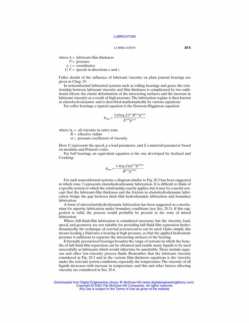
where h = lubricant-film thicknessP = pressure
x, z = coordinatesU, V = speeds in directions x and z
Fuller details of the influence of lubricant viscosity on plain journal bearings aregiven in Chap. 19.
In nonconformal lubricated systems such as rolling bearings and gears, the rela-tionship between lubricant viscosity and film thickness is complicated by two addi-tional effects: the elastic deformation of the interacting surfaces and the increase inlubricant viscosity as a result of high pressure. The lubrication regime is then knownas elastohydrodynamic and is described mathematically by various equations.
For roller bearings, a typical equation is the Dowson-Higginson equation:
hmin =
where ηo = oil viscosity in entry zoneR = effective radiusα = pressure coefficient of viscosity
Here U represents the speed, p a load parameter, and E a material parameter basedon modulus and Poisson’s ratio.
For ball bearings, an equivalent equation is the one developed by Archard andCowking:
hmin =
For such nonconformal systems, a diagram similar to Fig. 20.3 has been suggestedin which zone 2 represents elastohydrodynamic lubrication. It is difficult to think ofa specific system to which the relationship exactly applies, but it may be a useful con-cept that the lubricant-film thickness and the friction in elastohydrodynamic lubri-cation bridge the gap between thick-film hydrodynamic lubrication and boundarylubrication.
A form of microelastohydrodynamic lubrication has been suggested as a mecha-nism for asperity lubrication under boundary conditions (see Sec. 20.5). If this sug-gestion is valid, the process would probably be present in the zone of mixedlubrication.
Where full-fluid-film lubrication is considered necessary but the viscosity, load,speed, and geometry are not suitable for providing full-fluid-film separation hydro-dynamically, the technique of external pressurization can be used. Quite simply, thismeans feeding a fluid into a bearing at high pressure, so that the applied hydrostaticpressure is sufficient to separate the interacting surfaces of the bearing.
Externally pressurized bearings broaden the range of systems in which the bene-fits of full-fluid-film separation can be obtained and enable many liquids to be usedsuccessfully as lubricants which would otherwise be unsuitable. These include aque-ous and other low-viscosity process fluids. Remember that the lubricant viscosityconsidered in Fig. 20.3 and in the various film-thickness equations is the viscosityunder the relevant system conditions, especially the temperature.The viscosity of allliquids decreases with increase in temperature, and this and other factors affectingviscosity are considered in Sec. 20.4.
1.4(ηoUα)0.74E0.074
R0.74p0.074
2.65(ηoU)0.7R0.43α0.54
E0.03p0.13
LUBRICATION 20.5
LUBRICATION
Downloaded from Digital Engineering Library @ McGraw-Hill (www.digitalengineeringlibrary.com)Copyright © 2004 The McGraw-Hill Companies. All rights reserved.
Any use is subject to the Terms of Use as given at the website.
The viscosity and boundary lubrication properties of the lubricant completelydefine the lubrication performance, but many other properties are important in ser-vice. Most of these other properties are related to progressive deterioration of thelubricant; these are described in Sec. 20.6.
20.4 LUBRICANT VISCOSITY
Viscosity of lubricants is defined in two different ways, and unfortunately both defi-nitions are very widely used.
20.4.1 Dynamic or Absolute Viscosity
Dynamic or absolute viscosity is the ratio of the shear stress to the resultant shearrate when a fluid flows. In SI units it is measured in pascal-seconds or newton-seconds per square meter, but the centimeter-gram-second (cgs) unit, the centipoise,is more widely accepted, and
1 centipoise (cP) = 10−3 Pa ⋅ s = 10−3 N ⋅ s/m2
The centipoise is the unit of viscosity used in calculations based on the Reynoldsequation and the various elastohydrodynamic lubrication equations.
20.4.2 Kinematic Viscosity
The kinematic viscosity is equal to the dynamic viscosity divided by the density. TheSI unit is square meters per second, but the cgs unit, the centistoke, is more widelyaccepted, and
1 centistoke (cSt) = 1 mm2/s
The centistoke is the unit most often quoted by lubricant suppliers and users.In practice, the difference between kinematic and dynamic viscosities is not often
of major importance for lubricating oils, because their densities at operating tem-peratures usually lie between 0.8 and 1.2. However, for some fluorinated syntheticoils with high densities, and for gases, the difference can be very significant.
The viscosities of most lubricating oils are between 10 and about 600 cSt at theoperating temperature, with a median figure of about 90 cSt. Lower viscosities aremore applicable for bearings than for gears, as well as where the loads are light, thespeeds are high, or the system is fully enclosed. Conversely, higher viscosities areselected for gears and where the speeds are low, the loads are high, or the system iswell ventilated. Some typical viscosity ranges at the operating temperatures areshown in Table 20.1.
The variation of oil viscosity with temperature will be very important in somesystems, where the operating temperature either varies over a wide range or is verydifferent from the reference temperature for which the oil viscosity is quoted.
The viscosity of any liquid decreases as the temperature increases, but the rate ofdecrease can vary considerably from one liquid to another. Figure 20.4 shows the
20.6 BEARINGS AND LUBRICATION
LUBRICATION
Downloaded from Digital Engineering Library @ McGraw-Hill (www.digitalengineeringlibrary.com)Copyright © 2004 The McGraw-Hill Companies. All rights reserved.
Any use is subject to the Terms of Use as given at the website.
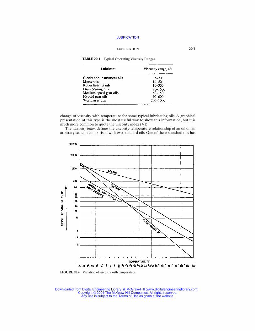
change of viscosity with temperature for some typical lubricating oils. A graphicalpresentation of this type is the most useful way to show this information, but it ismuch more common to quote the viscosity index (VI).
The viscosity index defines the viscosity-temperature relationship of an oil on anarbitrary scale in comparison with two standard oils. One of these standard oils has
LUBRICATION 20.7
TABLE 20.1 Typical Operating Viscosity Ranges
FIGURE 20.4 Variation of viscosity with temperature.
LUBRICATION
Downloaded from Digital Engineering Library @ McGraw-Hill (www.digitalengineeringlibrary.com)Copyright © 2004 The McGraw-Hill Companies. All rights reserved.
Any use is subject to the Terms of Use as given at the website.
a viscosity index of 0, representing the most rapid change of viscosity with tempera-ture normally found with any mineral oil. The second standard oil has a viscosityindex of 100, representing the lowest change of viscosity with temperature foundwith a mineral oil in the absence of relevant additives.
The equation for the calculation of the viscosity index of an oil sample is
VI = 100
L(L
−−H
U)
where U = viscosity of sample in centistokes at 40°C, L = viscosity in centistokes at40°C of oil of 0 VI having the same viscosity at 100°C as the test oil, and H = viscos-ity at 40°C of oil of 100 VI having the same viscosity at 100°C as the test oil.
Some synthetic oils can have viscosity indices of well over 150 by the above defi-nition, but the applicability of the definition at such high values is doubtful. The vis-cosity index of an oil can be increased by dissolving in it a quantity (sometimes ashigh as 20 percent) of a suitable polymer, called a viscosity index improver.
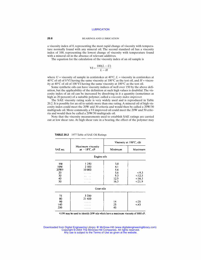
The SAE viscosity rating scale is very widely used and is reproduced in Table20.2. It is possible for an oil to satisfy more than one rating.A mineral oil of high vis-cosity index could meet the 20W and 30 criteria and would then be called a 20W/30multigrade oil. More commonly, a VI improved oil could meet the 20W and 50 crite-ria and would then be called a 20W/50 multigrade oil.
Note that the viscosity measurements used to establish SAE ratings are carriedout at low shear rate. At high shear rate in a bearing, the effect of the polymer may
20.8 BEARINGS AND LUBRICATION
TABLE 20.2 1977 Table of SAE Oil Ratings
LUBRICATION
Downloaded from Digital Engineering Library @ McGraw-Hill (www.digitalengineeringlibrary.com)Copyright © 2004 The McGraw-Hill Companies. All rights reserved.
Any use is subject to the Terms of Use as given at the website.
disappear, and a 20W/50 oil at very high shear rate may behave as a thinner oil thana 20W, namely, a 15W or even 10W. In practice, this may not be important, becausein a high-speed bearing the viscosity will probably still produce adequate oil-filmthickness.
Theoretically the viscosity index is important only where significant temperaturevariations apply, but in fact there is a tendency to use only high-viscosity-index oilsin the manufacture of high-quality lubricant. As a result, a high viscosity index isoften considered a criterion of lubricant quality, even where viscosity index as suchis of little or no importance.
Before we leave the subject of lubricant viscosity, perhaps some obsolescent vis-cosity units should be mentioned. These are the Saybolt viscosity (SUS) in NorthAmerica, the Redwood viscosity in the United Kingdom, and the Engler viscosity incontinental Europe. All three are of little practical utility, but have been very widelyused, and strenuous efforts have been made by standardizing organizations formany years to replace them entirely by kinematic viscosity.
20.5 BOUNDARY LUBRICATION
Boundary lubrication is important where there is significant solid-solid contactbetween sliding surfaces.To understand boundary lubrication, it is useful to first con-sider what happens when two metal surfaces slide against each other with no lubri-cant present.
In an extreme case, where the metal surfaces are not contaminated by an oxidefilm or any other foreign substance, there will be a tendency for the surfaces toadhere to each other. This tendency will be very strong for some pairs of metals andweaker for others. A few guidelines for common metals are as follows:
1. Identical metals in contact have a strong tendency to adhere.
2. Softer metals have a stronger tendency to adhere than harder metals.
3. Nonmetallic alloying elements tend to reduce adhesion (e.g., carbon in cast iron).
4. Iron and its alloys have a low tendency to adhere to lead, silver, tin, cadmium, andcopper and a high tendency to adhere to aluminum, zinc, titanium, and nickel.
Real metal surfaces are usually contaminated, especially by films of their ownoxides. Such contaminant films commonly reduce adhesion and thus reduce frictionand wear. Oxide films are particularly good lubricants, except for titanium.
Thus friction and wear can usually be reduced by deliberately generating suitablecontaminant films on metallic surfaces. Where no liquid lubricant is present, such aprocess is a type of dry or solid lubrication. Where the film-forming process takesplace in a liquid lubricant, it is called boundary lubrication.
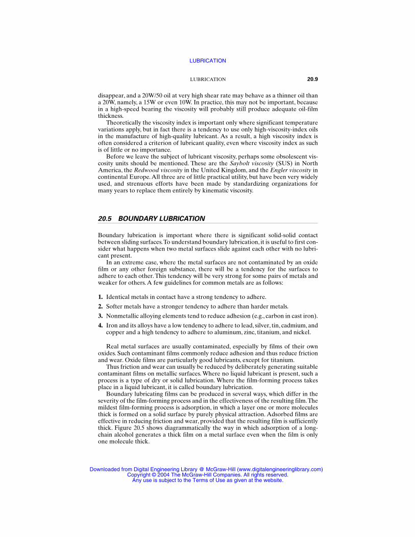
Boundary lubricating films can be produced in several ways, which differ in theseverity of the film-forming process and in the effectiveness of the resulting film.Themildest film-forming process is adsorption, in which a layer one or more moleculesthick is formed on a solid surface by purely physical attraction. Adsorbed films areeffective in reducing friction and wear, provided that the resulting film is sufficientlythick. Figure 20.5 shows diagrammatically the way in which adsorption of a long-chain alcohol generates a thick film on a metal surface even when the film is onlyone molecule thick.
LUBRICATION 20.9
LUBRICATION
Downloaded from Digital Engineering Library @ McGraw-Hill (www.digitalengineeringlibrary.com)Copyright © 2004 The McGraw-Hill Companies. All rights reserved.
Any use is subject to the Terms of Use as given at the website.
Mineral oils often contain small amounts of natural compounds which produceuseful adsorbed films. These compounds include unsaturated hydrocarbons (ole-fines) and nonhydrocarbons containing oxygen, nitrogen, or sulfur atoms (known asasphaltenes). Vegetable oils and animal fats also produce strong adsorbed films andmay be added in small concentrations to mineral oils for that reason. Other mildboundary additives include long-chain alcohols such as lauryl alcohol and esterssuch as ethyl stearate or ethyl oleate.
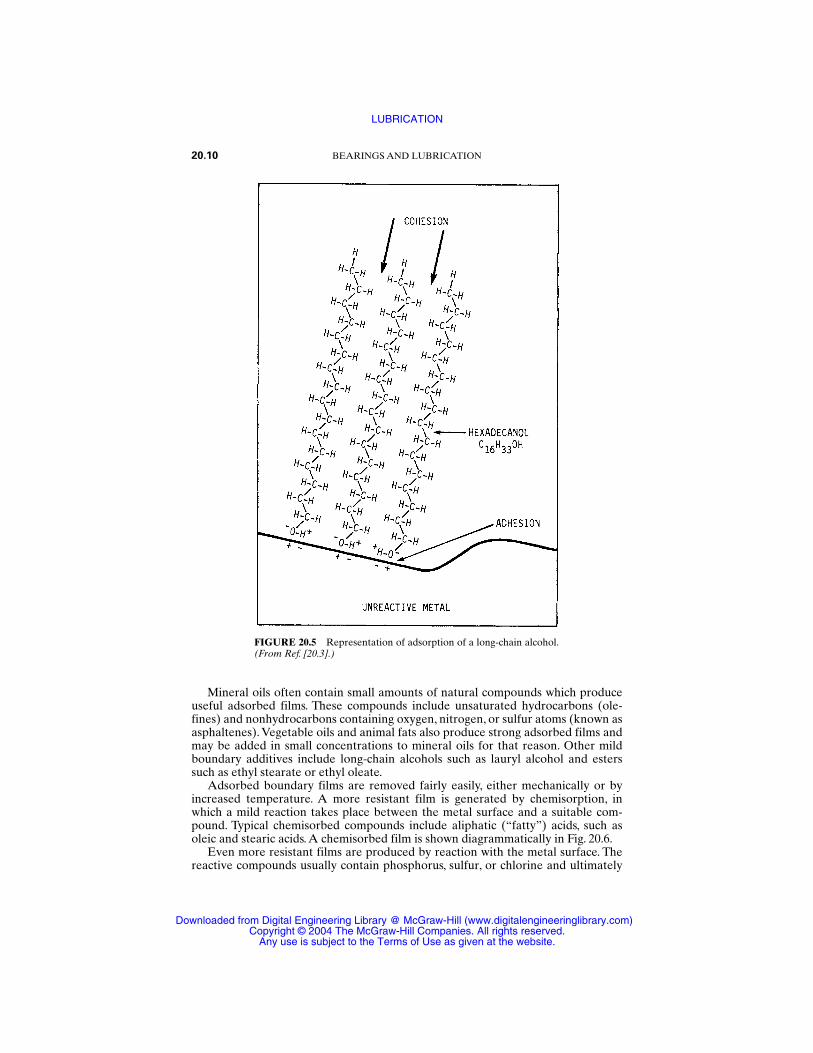
Adsorbed boundary films are removed fairly easily, either mechanically or byincreased temperature. A more resistant film is generated by chemisorption, inwhich a mild reaction takes place between the metal surface and a suitable com-pound. Typical chemisorbed compounds include aliphatic (“fatty”) acids, such asoleic and stearic acids. A chemisorbed film is shown diagrammatically in Fig. 20.6.
Even more resistant films are produced by reaction with the metal surface. Thereactive compounds usually contain phosphorus, sulfur, or chlorine and ultimately
20.10 BEARINGS AND LUBRICATION
FIGURE 20.5 Representation of adsorption of a long-chain alcohol.(From Ref. [20.3].)
LUBRICATION
Downloaded from Digital Engineering Library @ McGraw-Hill (www.digitalengineeringlibrary.com)Copyright © 2004 The McGraw-Hill Companies. All rights reserved.
Any use is subject to the Terms of Use as given at the website.
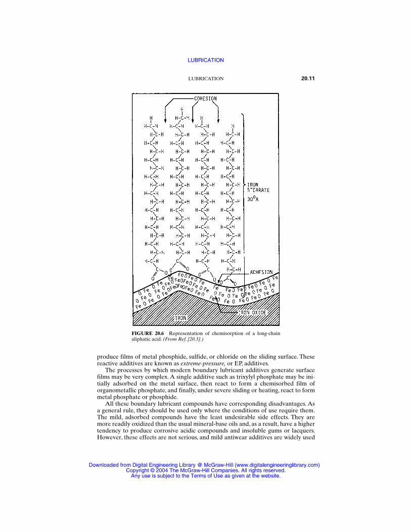
produce films of metal phosphide, sulfide, or chloride on the sliding surface. Thesereactive additives are known as extreme-pressure, or EP, additives.
The processes by which modern boundary lubricant additives generate surfacefilms may be very complex. A single additive such as trixylyl phosphate may be ini-tially adsorbed on the metal surface, then react to form a chemisorbed film oforganometallic phosphate, and finally, under severe sliding or heating, react to formmetal phosphate or phosphide.
All these boundary lubricant compounds have corresponding disadvantages. Asa general rule, they should be used only where the conditions of use require them.The mild, adsorbed compounds have the least undesirable side effects. They aremore readily oxidized than the usual mineral-base oils and, as a result, have a highertendency to produce corrosive acidic compounds and insoluble gums or lacquers.However, these effects are not serious, and mild antiwear additives are widely used
LUBRICATION 20.11
FIGURE 20.6 Representation of chemisorption of a long-chainaliphatic acid. (From Ref. [20.3].)
LUBRICATION
Downloaded from Digital Engineering Library @ McGraw-Hill (www.digitalengineeringlibrary.com)Copyright © 2004 The McGraw-Hill Companies. All rights reserved.
Any use is subject to the Terms of Use as given at the website.
in small quantities where sliding conditions are not severe, such as in hydraulic flu-ids and turbine oils.
The stronger chemisorbed additives such as fatty acids, organic phosphates, andthiophosphates are correspondingly more reactive. They are used in motor oils andgear oils. Finally, the reactive sulfurized olefines and chlorinated compounds are, infact, controlled corrodents and are used only where the sliding conditions are verysevere, such as in hypoid gearboxes and in metalworking processes.
Boundary lubrication is a very complex process. Apart from the direct film-forming techniques described earlier, there are several other effects which probablymake an important contribution to boundary lubrication:
1. The Rehbinder effect The presence of surface-active molecules adjacent to ametal surface decreases the yield stress. Since many boundary lubricants aremore or less surface-active, they can be expected to reduce the stresses devel-oped when asperities interact.
2. Viscosity increase adjacent to a metal surface This effect is controversial, but itseems probable that interaction between adsorbed molecules and the free ambi-ent oil can result in a greaselike thickening or trapping of oil molecules adjacentto the surface.
3. Microelastohydrodynamic effects The interaction between two asperities slid-ing past each other in a liquid is similar to the interaction between gear teeth, andin the same way it can be expected to generate elastohydrodynamic lubricationon a microscopic scale. The increase in viscosity of the lubricant and the elasticdeformation of the asperities will both tend to reduce friction and wear. How-ever, if the Rehbinder effect is also present, then plastic flow of the asperities isalso encouraged. The term microrheodynamic lubrication has been used todescribe this complex process.
4. Heating Even in well-lubricated sliding there will be transient heating effects atasperity interactions, and these will reduce the modulus and the yield stress atasperity interactions.
Boundary lubrication as a whole is not well understood, but the magnitude of itsbeneficial effects can be easily seen from the significant reductions in friction, wear,and seizure obtained with suitable liquid lubricants in slow metallic sliding.
20.6 DETERIORATION PROBLEMS
In theory, if the right viscosity and the right boundary properties have been selected,then the lubrication requirements will be met. In practice, there is one further com-plication—the oil deteriorates. Much of the technology of lubricating oils and addi-tives is concerned with reducing or compensating for deterioration.
The three important types of deterioration are oxidation, thermal decomposi-tion, and contamination.A fourth long-term effect is reaction with other materials inthe system, which is considered in terms of compatibility. Oxidation is the mostimportant deterioration process because over a long period, even at normal atmo-spheric temperature, almost all lubricants show some degree of oxidation.
Petroleum-base oils produced by mild refining techniques oxidize readily above120°C to produce acidic compounds, sludges, and lacquers. The total oxygen uptakeis not high, and this suggests that the trace compounds, such as aromatics and
20.12 BEARINGS AND LUBRICATION
LUBRICATION
Downloaded from Digital Engineering Library @ McGraw-Hill (www.digitalengineeringlibrary.com)Copyright © 2004 The McGraw-Hill Companies. All rights reserved.
Any use is subject to the Terms of Use as given at the website.
asphaltenes, are reacting, and that possibly in doing so some are acting as oxidationinhibitors for the paraffinic hydrocarbons present. Such mildly refined oils are notmuch improved by the addition of antioxidants.
More severe refining or hydrogenation produces a more highly paraffinic oilwhich absorbs oxygen more readily but without producing such harmful oxidationproducts. More important, however, the oxidation resistance of such highly refinedbase oils is very considerably improved by the addition of suitable oxidationinhibitors.
Most modern petroleum-base oils are highly refined in order to give consistentproducts with a wide operating-temperature range. Antioxidants are therefore animportant part of the formulation of almost all modern mineral-oil lubricants.
The commonly used antioxidants are amines, hindered phenols, organic phos-phites, and organometallic compounds. One particularly important additive is zincdiethyl dithiophosphate, which is a very effective antioxidant and also has usefulboundary lubrication and corrosion-inhibition properties.
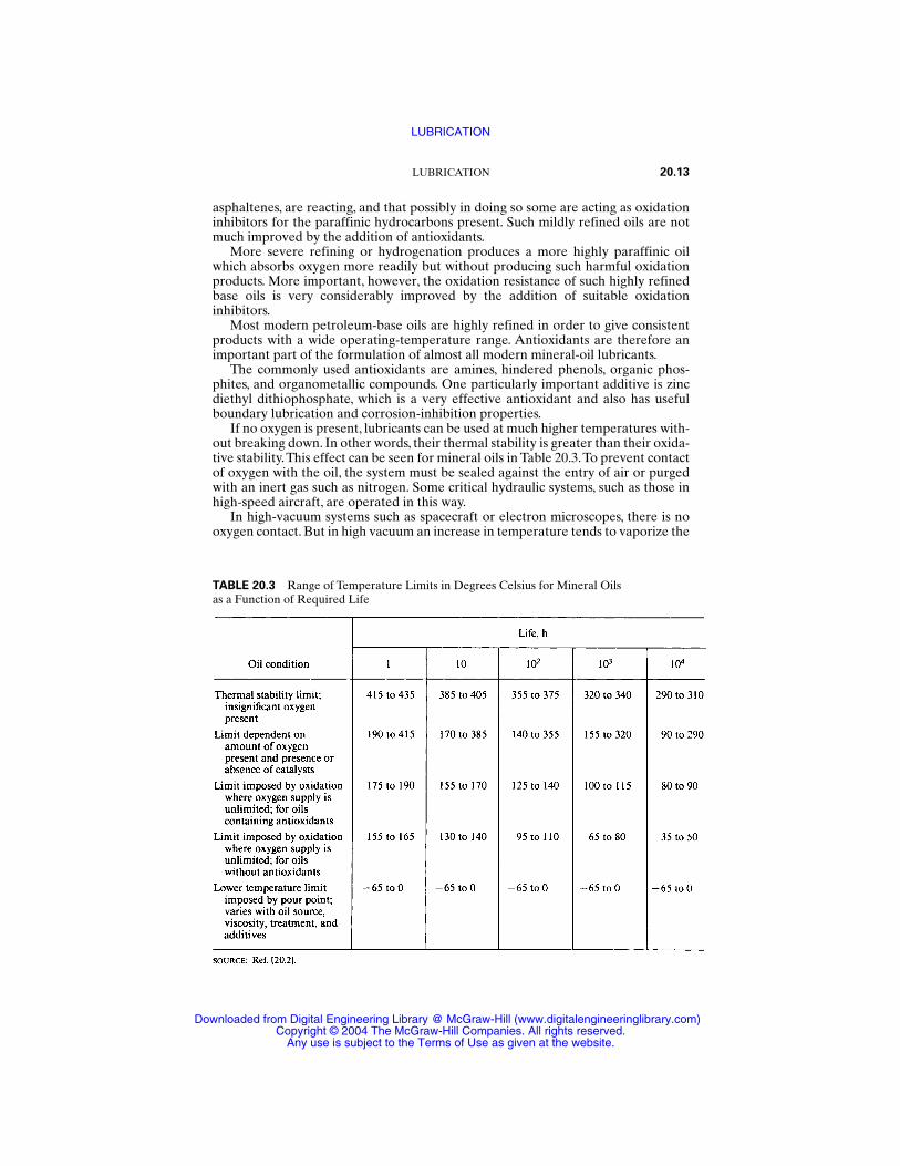
If no oxygen is present, lubricants can be used at much higher temperatures with-out breaking down. In other words, their thermal stability is greater than their oxida-tive stability.This effect can be seen for mineral oils in Table 20.3.To prevent contactof oxygen with the oil, the system must be sealed against the entry of air or purgedwith an inert gas such as nitrogen. Some critical hydraulic systems, such as those inhigh-speed aircraft, are operated in this way.
In high-vacuum systems such as spacecraft or electron microscopes, there is nooxygen contact. But in high vacuum an increase in temperature tends to vaporize the
LUBRICATION 20.13
TABLE 20.3 Range of Temperature Limits in Degrees Celsius for Mineral Oils as a Function of Required Life
LUBRICATION
Downloaded from Digital Engineering Library @ McGraw-Hill (www.digitalengineeringlibrary.com)Copyright © 2004 The McGraw-Hill Companies. All rights reserved.
Any use is subject to the Terms of Use as given at the website.
oil, so that high thermal stability is of little or no value. It follows that oxidative sta-bility is usually much more important than thermal stability.
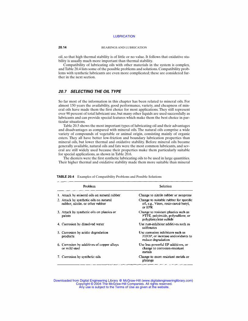
Compatibility of lubricating oils with other materials in the system is complex,and Table 20.4 lists some of the possible problems and solutions. Compatibility prob-lems with synthetic lubricants are even more complicated; these are considered fur-ther in the next section.
20.7 SELECTING THE OIL TYPE
So far most of the information in this chapter has been related to mineral oils. Foralmost 150 years the availability, good performance, variety, and cheapness of min-eral oils have made them the first choice for most applications. They still representover 90 percent of total lubricant use, but many other liquids are used successfully aslubricants and can provide special features which make them the best choice in par-ticular situations.
Table 20.5 shows the most important types of lubricating oil and their advantagesand disadvantages as compared with mineral oils. The natural oils comprise a widevariety of compounds of vegetable or animal origin, consisting mainly of organicesters. They all have better low-friction and boundary lubrication properties thanmineral oils, but lower thermal and oxidative stability. Before mineral oils becamegenerally available, natural oils and fats were the most common lubricants, and sev-eral are still widely used because their properties make them particularly suitablefor special applications, as shown in Table 20.6.
The diesters were the first synthetic lubricating oils to be used in large quantities.Their higher thermal and oxidative stability made them more suitable than mineral
20.14 BEARINGS AND LUBRICATION
TABLE 20.4 Examples of Compatibility Problems and Possible Solutions
LUBRICATION
Downloaded from Digital Engineering Library @ McGraw-Hill (www.digitalengineeringlibrary.com)Copyright © 2004 The McGraw-Hill Companies. All rights reserved.
Any use is subject to the Terms of Use as given at the website.

LUBRICATION 20.15
TABLE 20.5 Advantages and Disadvantages of Main Nonmineral Oils
TABLE 20.6 Some Uses of Natural Oils and Fats
LUBRICATION
Downloaded from Digital Engineering Library @ McGraw-Hill (www.digitalengineeringlibrary.com)Copyright © 2004 The McGraw-Hill Companies. All rights reserved.
Any use is subject to the Terms of Use as given at the website.
oils for gas-turbine lubrication, and by about 1960 they were almost universally usedfor aircraft jet engines. For the even more demanding conditions of supersonic jetengines, the more complex ester lubricants such as hindered phenols and triesterswere developed.
Phosphate esters and chlorinated diphenyls have very low-flammability charac-teristics, and this has led to their wide use where critical fire-risk situations occur,such as in aviation and coal mining. Their overall properties are mediocre, but aresufficiently good for use where fire resistance is particularly important.
Other synthetic fluids such as silicones, chlorinated silicones, fluorinated sili-cones, fluorinated hydrocarbon, and polyphenyl ethers are all used in relativelysmall quantities for their high-temperature stability, but all are inferior lubricantsand very expensive compared with mineral oils.
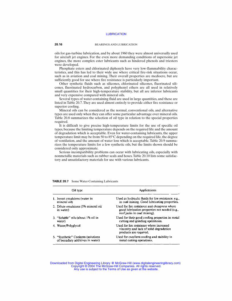
Several types of water-containing fluid are used in large quantities, and these arelisted in Table 20.7. They are used almost entirely to provide either fire resistance orsuperior cooling.
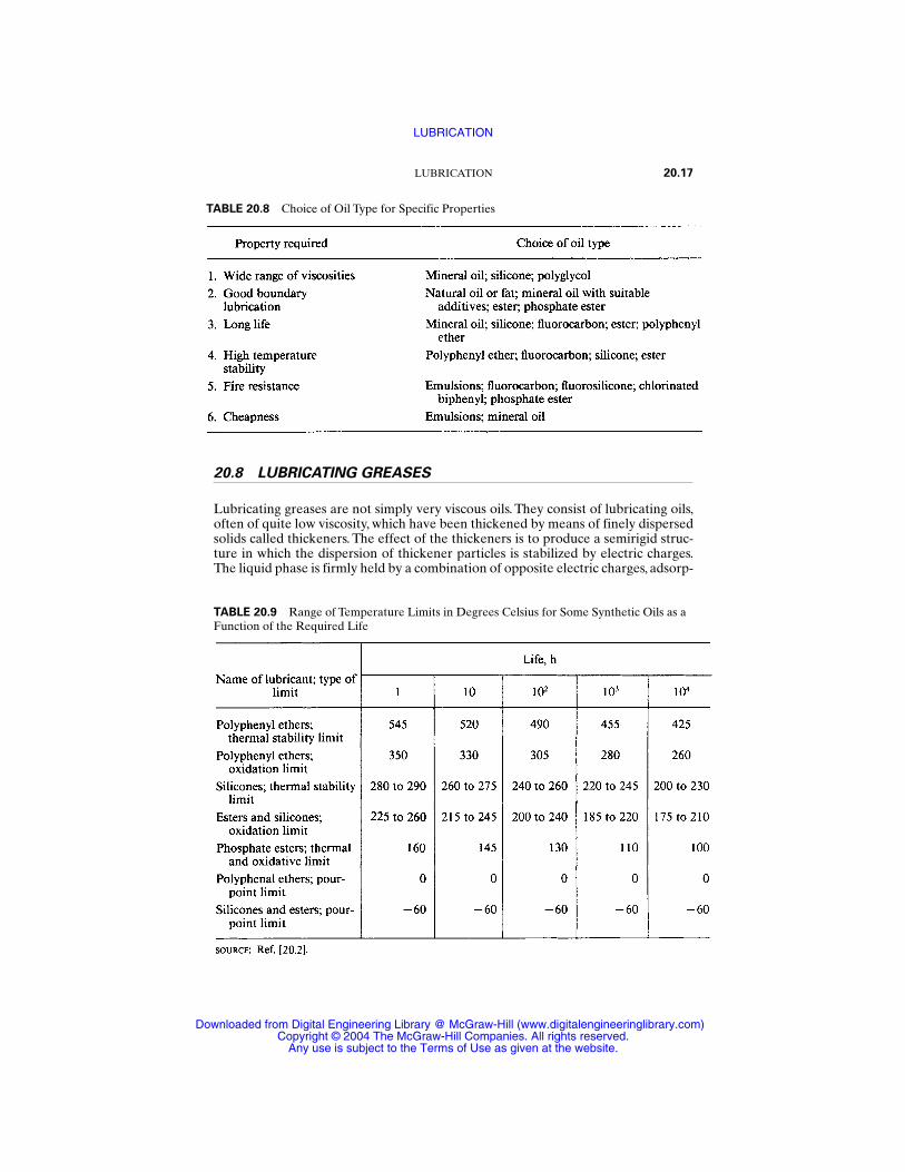
Mineral oils can be considered as the normal, conventional oils, and alternativetypes are used only when they can offer some particular advantage over mineral oils.Table 20.8 summarizes the selection of oil type in relation to the special propertiesrequired.
It is difficult to give precise high-temperature limits for the use of specific oiltypes, because the limiting temperature depends on the required life and the amountof degradation which is acceptable. Even for water-containing lubricants, the uppertemperature limit may be from 50 to 85°C depending on the required life, the degreeof ventilation, and the amount of water loss which is acceptable. Table 20.9 summa-rizes the temperature limits for a few synthetic oils, but the limits shown should beconsidered only approximate.
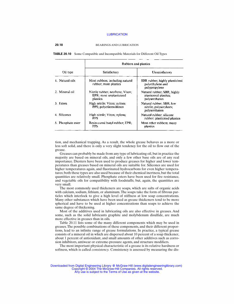
Serious incompatibility problems can occur with lubricating oils, especially withnonmetallic materials such as rubber seals and hoses. Table 20.10 lists some satisfac-tory and unsatisfactory materials for use with various lubricants.
20.16 BEARINGS AND LUBRICATION
TABLE 20.7 Some Water-Containing Lubricants
LUBRICATION
Downloaded from Digital Engineering Library @ McGraw-Hill (www.digitalengineeringlibrary.com)Copyright © 2004 The McGraw-Hill Companies. All rights reserved.
Any use is subject to the Terms of Use as given at the website.
20.8 LUBRICATING GREASES
Lubricating greases are not simply very viscous oils. They consist of lubricating oils,often of quite low viscosity, which have been thickened by means of finely dispersedsolids called thickeners. The effect of the thickeners is to produce a semirigid struc-ture in which the dispersion of thickener particles is stabilized by electric charges.The liquid phase is firmly held by a combination of opposite electric charges, adsorp-
LUBRICATION 20.17
TABLE 20.8 Choice of Oil Type for Specific Properties
TABLE 20.9 Range of Temperature Limits in Degrees Celsius for Some Synthetic Oils as aFunction of the Required Life
LUBRICATION
Downloaded from Digital Engineering Library @ McGraw-Hill (www.digitalengineeringlibrary.com)Copyright © 2004 The McGraw-Hill Companies. All rights reserved.
Any use is subject to the Terms of Use as given at the website.
tion, and mechanical trapping. As a result, the whole grease behaves as a more orless soft solid, and there is only a very slight tendency for the oil to flow out of thegrease.
Greases can probably be made from any type of lubricating oil, but in practice themajority are based on mineral oils, and only a few other base oils are of any realimportance. Diesters have been used to produce greases for higher and lower tem-peratures than greases based on mineral oils are suitable for. Silicones are used forhigher temperatures again, and fluorinated hydrocarbons for even higher tempera-tures; both these types are also used because of their chemical inertness, but the totalquantities are relatively small. Phosphate esters have been used for fire resistance,and vegetable oils for compatibility with foodstuffs; but, again, the quantities arevery small.
The most commonly used thickeners are soaps, which are salts of organic acidswith calcium, sodium, lithium, or aluminum. The soaps take the form of fibrous par-ticles which interlock to give a high level of stiffness at low soap concentrations.Many other substances which have been used as grease thickeners tend to be morespherical and have to be used at higher concentrations than soaps to achieve thesame degree of thickening.
Most of the additives used in lubricating oils are also effective in greases. Andsome, such as the solid lubricants graphite and molybdenum disulfide, are muchmore effective in greases than in oils.
Table 20.11 lists some of the many different components which may be used ingreases. The possible combinations of these components, and their different propor-tions, lead to an infinite range of grease formulations. In practice, a typical greaseconsists of a mineral oil in which are dispersed about 10 percent of a soap thickener,about 1 percent of antioxidant, and small amounts of other additives such as corro-sion inhibitors, antiwear or extreme-pressure agents, and structure modifiers.
The most important physical characteristic of a grease is its relative hardness orsoftness, which is called consistency. Consistency is assessed by measuring the dis-
20.18 BEARINGS AND LUBRICATION
TABLE 20.10 Some Compatible and Incompatible Materials for Different Oil Types
LUBRICATION
Downloaded from Digital Engineering Library @ McGraw-Hill (www.digitalengineeringlibrary.com)Copyright © 2004 The McGraw-Hill Companies. All rights reserved.
Any use is subject to the Terms of Use as given at the website.
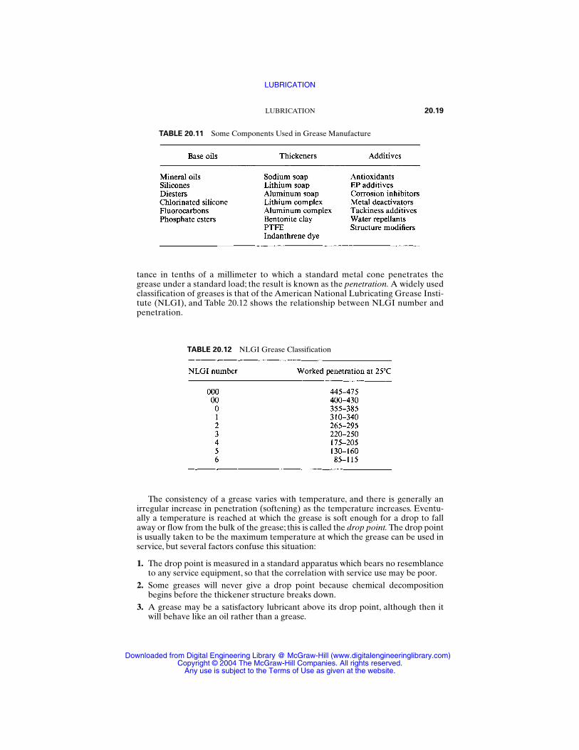
tance in tenths of a millimeter to which a standard metal cone penetrates thegrease under a standard load; the result is known as the penetration. A widely usedclassification of greases is that of the American National Lubricating Grease Insti-tute (NLGI), and Table 20.12 shows the relationship between NLGI number andpenetration.
LUBRICATION 20.19
TABLE 20.11 Some Components Used in Grease Manufacture
TABLE 20.12 NLGI Grease Classification
The consistency of a grease varies with temperature, and there is generally anirregular increase in penetration (softening) as the temperature increases. Eventu-ally a temperature is reached at which the grease is soft enough for a drop to fallaway or flow from the bulk of the grease; this is called the drop point. The drop pointis usually taken to be the maximum temperature at which the grease can be used inservice, but several factors confuse this situation:
1. The drop point is measured in a standard apparatus which bears no resemblanceto any service equipment, so that the correlation with service use may be poor.
2. Some greases will never give a drop point because chemical decompositionbegins before the thickener structure breaks down.
3. A grease may be a satisfactory lubricant above its drop point, although then itwill behave like an oil rather than a grease.
LUBRICATION
Downloaded from Digital Engineering Library @ McGraw-Hill (www.digitalengineeringlibrary.com)Copyright © 2004 The McGraw-Hill Companies. All rights reserved.
Any use is subject to the Terms of Use as given at the website.
4. Some greases can be heated above their drop points and will again form a greasewhen cooled, although normally the re-formed grease will be markedly inferiorin properties.
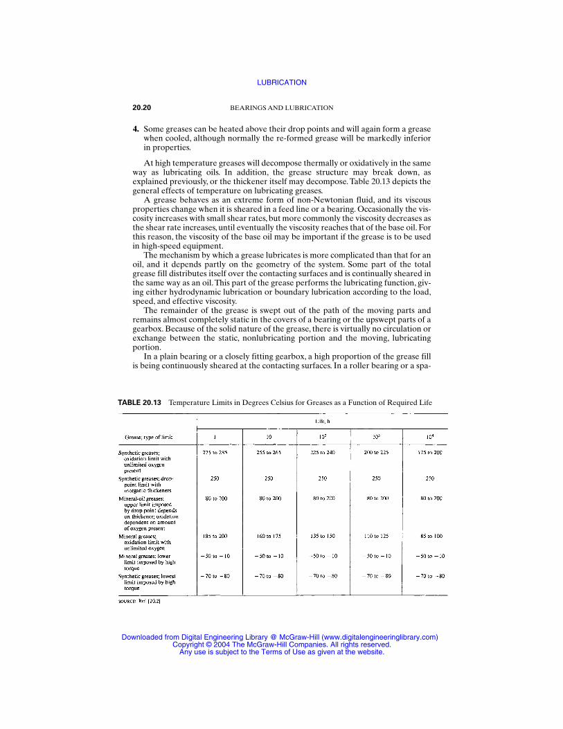
At high temperature greases will decompose thermally or oxidatively in the sameway as lubricating oils. In addition, the grease structure may break down, asexplained previously, or the thickener itself may decompose. Table 20.13 depicts thegeneral effects of temperature on lubricating greases.
A grease behaves as an extreme form of non-Newtonian fluid, and its viscousproperties change when it is sheared in a feed line or a bearing. Occasionally the vis-cosity increases with small shear rates, but more commonly the viscosity decreases asthe shear rate increases, until eventually the viscosity reaches that of the base oil. Forthis reason, the viscosity of the base oil may be important if the grease is to be usedin high-speed equipment.
The mechanism by which a grease lubricates is more complicated than that for anoil, and it depends partly on the geometry of the system. Some part of the totalgrease fill distributes itself over the contacting surfaces and is continually sheared inthe same way as an oil.This part of the grease performs the lubricating function, giv-ing either hydrodynamic lubrication or boundary lubrication according to the load,speed, and effective viscosity.
The remainder of the grease is swept out of the path of the moving parts andremains almost completely static in the covers of a bearing or the upswept parts of agearbox. Because of the solid nature of the grease, there is virtually no circulation orexchange between the static, nonlubricating portion and the moving, lubricatingportion.
In a plain bearing or a closely fitting gearbox, a high proportion of the grease fillis being continuously sheared at the contacting surfaces. In a roller bearing or a spa-
20.20 BEARINGS AND LUBRICATION
TABLE 20.13 Temperature Limits in Degrees Celsius for Greases as a Function of Required Life
LUBRICATION
Downloaded from Digital Engineering Library @ McGraw-Hill (www.digitalengineeringlibrary.com)Copyright © 2004 The McGraw-Hill Companies. All rights reserved.
Any use is subject to the Terms of Use as given at the website.

cious gearbox, a small proportion of the grease is continuously sheared and providesall the lubrication, while the larger proportion is inactive.
If a rolling bearing or gearbox is overfilled with grease, it may be impossible forthe surplus to escape from the moving parts. Then a large quantity of grease will becontinuously sheared, or “churned,” and this causes a buildup of temperature whichcan severely damage the grease and the components. It is, therefore, important withgrease lubrication to leave a void space which is sufficient to accommodate all thesurplus grease; in a ball bearing, this could be more than 60 percent of the total spaceavailable.
The static grease which is not involved in lubrication may fulfill two useful func-tions: It may provide a very effective seal against the ingress of dust or other con-taminants, and it can prevent loss of base oil from the grease fill. In addition, thestatic grease may form a reservoir from which to resupply the lubricated surfaces ifthe lubricating portion of the grease becomes depleted.
If the void space in the system is large, i.e., in a large bearing or gearbox, then usu-ally it is desirable to use a stiffer grease to avoid the surplus grease “slumping” intothe moving parts and being continuously churned. The advantages and disadvan-tages of grease lubrication are summarized in Table 20.14.
The selection of a grease for a specific application depends on five factors: speed,load, size, temperature range, and any grease feed system. For average conditions ofspeed, load, and size with no feed system, an NLGI no. 2 grease would be the normalchoice, and such a grease with a mineral-oil base is sometimes known as a multipur-pose grease.The effect of the various factors on selection can then be summarized ina few paragraphs.
1. Speed For high speeds, a stiffer grease, NLGI no. 3, should be used except inplain bearings, where no. 2 would usually be hard enough. For lower speeds, asofter grease such as no. 1 or no. 0 should be used.
LUBRICATION 20.21
TABLE 20.14 Advantages and Disadvantages of Grease Lubrication
LUBRICATION
Downloaded from Digital Engineering Library @ McGraw-Hill (www.digitalengineeringlibrary.com)Copyright © 2004 The McGraw-Hill Companies. All rights reserved.
Any use is subject to the Terms of Use as given at the website.
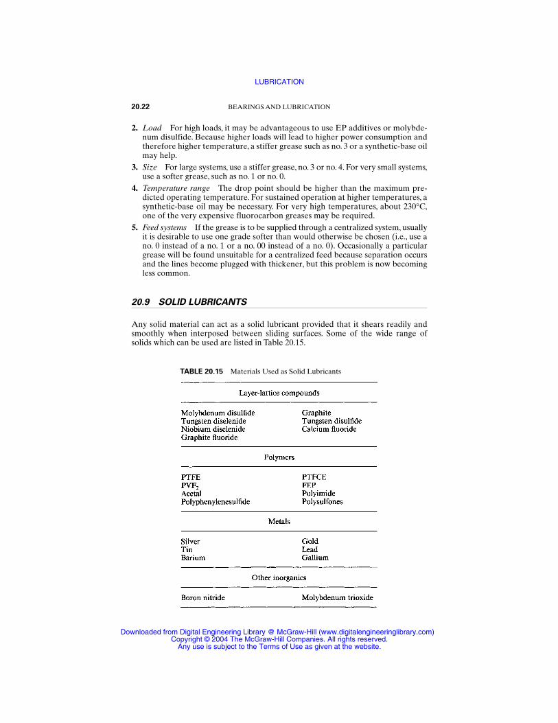
2. Load For high loads, it may be advantageous to use EP additives or molybde-num disulfide. Because higher loads will lead to higher power consumption andtherefore higher temperature, a stiffer grease such as no. 3 or a synthetic-base oilmay help.
3. Size For large systems, use a stiffer grease, no. 3 or no. 4. For very small systems,use a softer grease, such as no. 1 or no. 0.
4. Temperature range The drop point should be higher than the maximum pre-dicted operating temperature. For sustained operation at higher temperatures, asynthetic-base oil may be necessary. For very high temperatures, about 230°C,one of the very expensive fluorocarbon greases may be required.
5. Feed systems If the grease is to be supplied through a centralized system, usuallyit is desirable to use one grade softer than would otherwise be chosen (i.e., use ano. 0 instead of a no. 1 or a no. 00 instead of a no. 0). Occasionally a particulargrease will be found unsuitable for a centralized feed because separation occursand the lines become plugged with thickener, but this problem is now becomingless common.
20.9 SOLID LUBRICANTS
Any solid material can act as a solid lubricant provided that it shears readily andsmoothly when interposed between sliding surfaces. Some of the wide range ofsolids which can be used are listed in Table 20.15.
20.22 BEARINGS AND LUBRICATION
TABLE 20.15 Materials Used as Solid Lubricants
LUBRICATION
Downloaded from Digital Engineering Library @ McGraw-Hill (www.digitalengineeringlibrary.com)Copyright © 2004 The McGraw-Hill Companies. All rights reserved.
Any use is subject to the Terms of Use as given at the website.
There are many other desirable properties, including the following:
1. Ability to adhere to one or both of the bearing surfaces to ensure retention in thecontact area
2. Chemical stability over the required temperature range in the particular envi-ronment
3. Sufficient resistance to wear4. Nontoxicity5. Easy application6. Economy
Most of the available materials are eliminated by these requirements, and inpractice almost all solid lubrication in engineering is provided by three materials—graphite, molybdenum disulfide, and polytetrafluoroethylene (PTFE).
Solid lubricants can be used in several different forms, such as loose powder,adhering powder, bonded film, or solid block. In the form of a solid block, the mate-rial is often called a dry bearing material rather than a solid lubricant.
20.9.1 Graphite
Graphite is probably the oldest known of the three main solid lubricants, and it hasceased to be the dominant one since about 1950. It is a grayish black crystalline formof carbon in which the atoms are arranged hexagonally in monatomic layers. Thestrong chemical bonds between the carbon atoms give strength to the layers, so thatthey resist bending or fracture and can carry useful loads. The bonds between thelayers are relatively weak, and so the layers slide easily over each other and can beeasily separated.
When graphite is used as a lubricant, the crystals orient themselves so that thelayers are parallel to the bearing surfaces. The layers then adhere fairly well to thebearing surfaces, but slide easily over each other to give low friction.
The low shearing forces, and therefore the low friction, are not an inherent prop-erty of the graphite but are strongly influenced by the presence of moisture or cer-tain other adsorbents. If graphite is used in a very dry atmosphere, the crystal layershave quite high interlayer bonding forces, and the friction and wear are high.
The biggest advantage of graphite over molybdenum disulfide and PTFE is itselectrical conductivity, and it is almost universally used as a component in electricbrushes. Its coefficient of friction varies from 0.05 at high loads to 0.15 at low loads,and these low values are maintained to over 500°C in air.
In block form, graphite has quite high structural integrity. It is commonly used inan impure form as graphitized carbon, in which the degree of crystallization can varyfrom 30 to over 80 percent of that of crystalline graphite. The frictional and struc-tural properties and abrasiveness vary with the purity and degree of graphitization,and graphite technology is complex.
Graphite can be used in block form, as free powder, or as a coating depositedfrom dispersion in a liquid. It adheres readily to many solid surfaces, but probably itsstrength of adhesion is generally lower than that of molybdenum disulfide.
20.9.2 Molybdenum Disulfide
Molybdenum disulfide has also been known as a solid lubricant for centuries, butbecause it is similar in appearance, it has often been confused with graphite. Its use
LUBRICATION 20.23
LUBRICATION
Downloaded from Digital Engineering Library @ McGraw-Hill (www.digitalengineeringlibrary.com)Copyright © 2004 The McGraw-Hill Companies. All rights reserved.
Any use is subject to the Terms of Use as given at the website.
has increased enormously since about 1950, and for high-technology applications itis now generally preferred to graphite. In crude form, molybdenum disulfide isfound naturally, sometimes in very large quantities, as molybdenite, the most com-mon ore of molybdenum.
Like graphite, molybdenum disulfide is a dark gray crystalline material with ahexagonal layer-lattice structure.The bond strengths within the layers are very high,whereas those between layers are very low.The load-carrying capacity normal to thecrystal planes is therefore high, and the shear strength parallel to the crystal layers isvery low.
Unlike graphite, molybdenum disulfide does not require the presence ofadsorbed moisture or other vapors to give low interplanar strength. Its low frictionis therefore an inherent property which is maintained in high vacuum and in dryatmospheres.
Molybdenum disulfide starts to oxidize significantly above 350°C in oxygen and450°C in air, but the main oxidation product is molybdic oxide, which is itself a fairhigh-temperature lubricant. In high vacuum the disulfide is said to be stable to1000°C, and it outgasses (evaporates) very slowly, so that it has been widely used inspace.
The adhesion to metals and many other solid surfaces is excellent, and durablecoatings can be produced on metal surfaces by burnishing (a coating of loose pow-der is rubbed into the surface to give a very thin, shiny, and strong film).The powdermay be applied free or from dispersion in a volatile liquid. Durable coatings can alsobe obtained by sputtering, but this technique is expensive and is not widely used.
Bonded coatings are widely used, in which molybdenum disulfide powder isincorporated in almost any effective adhesive, including many polymers, naturalresins, or molten solids. The performance of the softer bonded coatings is alsoimproved if they are carefully burnished before use. The coefficient of friction ofburnished films varies from 0.02 to about 0.12. But for bonded films the frictiondepends on the nature of the binder and the percentage composition, and it can varyfrom 0.02 to about 0.3.
Molybdenum disulfide is often added to oils or greases to give high load-carryingcapacity, especially at low running speeds. There is also strong evidence that theaddition of up to 2 percent to vehicle engine oils produces a small but significant fuelsavings without any apparent disadvantages.
At one time molybdenum disulfide suffered considerable criticism, especially forreported corrosion of steels and aluminum. Some of this may have been due to itsuse in conjunction with graphite. Some was certainly caused by failure to understandthat solid lubricants, unlike oils and greases, do not normally protect against corro-sion. It is probably fair to say that molybdenum disulfide is now well understood andthat, when properly used, it is a very valuable solid lubricant.
20.9.3 Polytetrafluoroethylene
Abbreviated PTFE, polytetrafluoroethylene is a polymer produced from ethylenein which all the hydrogen atoms have been replaced by fluorine atoms. This fluori-nation produces a material of very high chemical stability and low intermolecularbond strength, while the polymerization of an ethylene-type molecule gives long,straight molecular chains.
The result is a white solid which consists of masses of parallel long-chainmolecules that slide easily past one another. This leads to the same sort of low shearstrength parallel to the chains which is found in molybdenum disulfide and to a high
20.24 BEARINGS AND LUBRICATION
LUBRICATION
Downloaded from Digital Engineering Library @ McGraw-Hill (www.digitalengineeringlibrary.com)Copyright © 2004 The McGraw-Hill Companies. All rights reserved.
Any use is subject to the Terms of Use as given at the website.
load-carrying capacity normal to the chains, but significantly lower than that ofmolybdenum disulfide.
PTFE is often used in the form of solid components, occasionally in bonded coat-ings, and very rarely as free powder. In addition, it has been used very successfully incomposites, and two types are particularly effective.
The coefficient of friction of pure PTFE varies from 0.02 at high load to about 0.1at low load. It is a rather soft solid, so that its load-carrying capacity is limited and itswear rate is high. It therefore needs reinforcement for use in highly loaded bearings.One successful form of reinforcement is to incorporate the PTFE in the pores of asintered metal, especially bronze. In one composite, further reinforcement isobtained by dispersing fine particles of lead in the PTFE.
A second, and probably even more successful, form of reinforcement is by meansof strengthening fibers. Glass fiber or carbon fiber can be incorporated in solidPTFE components, but the resulting high structural strength is obtained at the costof an increase in the coefficient of friction to between 0.06 and 0.2. An alternativetechnique is to interweave PTFE fibers and reinforcing fibers of glass, metal, rayon,or other synthetics. Some of the resulting composites have outstanding strength withlow wear rate and low friction.
PTFE can be used in air to about 250°C, but in high vacuum it outgasses slowly,and so it is used in spacecraft only in well-shielded locations.
Because of its high chemical stability, PTFE can be used safely in oxygen systemsand in many types of chemical plants. It is nontoxic in almost all situations and istherefore used in the pharmaceutical and food industries, even in situations where lowfriction is not required, and as the nonstick lubricant in domestic cooking utensils.
20.9.4 Miscellaneous Solid Lubricants
Other solid lubricants are used to a relatively minor degree, in situations where theyhave specific advantages. They can be classified in three broad categories: inorgan-ics, polymers, and metals.
The inorganics include a number of materials similar to molybdenum disulfide,known generally as the lubricating dichalcogenides. None of these occurs naturally,and the synthetic materials are relatively expensive. Tungsten disulfide has a higheroxidation temperature, and both tungsten disulfide and tungsten diselenide oxidizemore slowly than molybdenum disulfide. Niobium diselenide has better electricalconductivity and has been used in electric contact brushes, but in fact molybdenumdisulfide composites have been shown to be equally satisfactory.
Other inorganics have been used for their much higher temperature limits, andthese include molybdic oxide, boron nitride, graphite fluoride, and calcium fluoride.
The low friction and chemical inertness of PTFE make it difficult to bond toother materials, and two other fluorinated polymers have been recommended fortheir better bonding behavior: polyvinylfluoride (PVF2) and polytrifluorochlo-roethylene (PTFCE). But in both cases the advantages of better bonding andslightly higher structural strength are offset by higher friction.
For higher temperatures, polyimide, polysulfones, and polyphenylene sulfide canbe used unlubricated. Other polymers, such as nylons, acetals, and phenolics, areoccasionally used unlubricated where sliding speeds are low, but they require lubri-cation by oil, grease, or water for really useful performance.
Silver, gold, and tin have useful antigalling properties in slow sliding, but metalliccoatings are mainly used as lubricants only in high vacuum, where silver, gold, bar-ium, gallium, and lead have all been used successfully.
LUBRICATION 20.25
LUBRICATION
Downloaded from Digital Engineering Library @ McGraw-Hill (www.digitalengineeringlibrary.com)Copyright © 2004 The McGraw-Hill Companies. All rights reserved.
Any use is subject to the Terms of Use as given at the website.
20.10 GAS LUBRICATION
Gases can be used to provide full-fluid-film lubrication in the same ways as liquidsin hydrodynamic and externally pressurized bearings. The physical laws governingbehavior are the same for both liquids and gases, but the very low viscosities of gaseslead to considerable practical differences in their use, especially in self-pressurizing,or “gas-dynamic,” bearings:
1. Operating speeds are much higher to compensate for low viscosity.2. Surface finish and precision must be better because of the much smaller lubricant-
film thickness.3. Lubricant flow rate is higher for the same pressure differential.4. Load-carrying capacity is generally low.
As a result, gas bearings tend to be small, high-speed, and lightly loaded, withtight tolerances and high-quality surface finishes. The overall design and manufac-turing cost is high, and they are mainly used in high-technology applications.
Any gas or vapor can be used provided that it is chemically stable under the oper-ating conditions and does not attack any of the system materials. If no chemicalchange takes place, there is no upper temperature limit to the use of a gas, and theviscosity increases as temperature increases.
Air is the most common gas used in gas lubrication. Nitrogen or helium may beused where inertness is important. Otherwise, any gas which is available can be used,especially if it is available at high enough pressure for external pressurization.
Some of the advantages of gas lubrication are high precision, very low friction,cleanliness, and ready availability of lubricant. The greatest potential advantage isthe wide temperature range. In theory, it should be possible to design a gas bearingto operate from −250 to +2000°C. The corresponding disadvantages include thedemanding design and construction requirements, the low load-carrying capacity,and the need for a very clean gas supply. Examples of important applications of gasbearings are dentists’ air-turbine drills, high-precision grinding spindles, and inertialgyroscopes.
20.11 LUBRICANT FEED SYSTEMS
In many lubricated components, no feed system is needed, because the initial lubri-cant fill is sufficient to last the required life. A feed system becomes necessary whenthe lubricant must be replaced or replenished, for one of the following reasons:
1. The temperature is too high, so that the lubricant must be removed and replacedby a fresh charge of cooler lubricant.
2. Lubricant becomes depleted by leakage or creepage and must be topped up.3. Lubricant decomposes and must be replaced with a fresh charge.4. Lubricant becomes contaminated and must be replaced with clean material.
Where the rate of loss or deterioration is relatively low, it will be sufficient to pro-vide a facility for occasional topping up by means of an oil can or a grease gun, pro-vided that access to the lubricated component is available. Where this occasionalmanual topping up is not adequate, a lubricant feed system will be needed. It is
20.26 BEARINGS AND LUBRICATION
LUBRICATION
Downloaded from Digital Engineering Library @ McGraw-Hill (www.digitalengineeringlibrary.com)Copyright © 2004 The McGraw-Hill Companies. All rights reserved.
Any use is subject to the Terms of Use as given at the website.
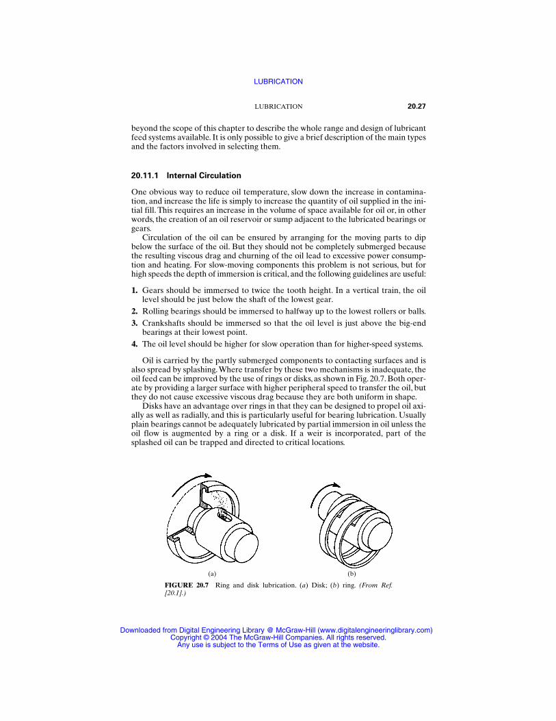
beyond the scope of this chapter to describe the whole range and design of lubricantfeed systems available. It is only possible to give a brief description of the main typesand the factors involved in selecting them.
20.11.1 Internal Circulation
One obvious way to reduce oil temperature, slow down the increase in contamina-tion, and increase the life is simply to increase the quantity of oil supplied in the ini-tial fill. This requires an increase in the volume of space available for oil or, in otherwords, the creation of an oil reservoir or sump adjacent to the lubricated bearings orgears.
Circulation of the oil can be ensured by arranging for the moving parts to dipbelow the surface of the oil. But they should not be completely submerged becausethe resulting viscous drag and churning of the oil lead to excessive power consump-tion and heating. For slow-moving components this problem is not serious, but forhigh speeds the depth of immersion is critical, and the following guidelines are useful:
1. Gears should be immersed to twice the tooth height. In a vertical train, the oillevel should be just below the shaft of the lowest gear.
2. Rolling bearings should be immersed to halfway up to the lowest rollers or balls.3. Crankshafts should be immersed so that the oil level is just above the big-end
bearings at their lowest point.4. The oil level should be higher for slow operation than for higher-speed systems.
Oil is carried by the partly submerged components to contacting surfaces and isalso spread by splashing.Where transfer by these two mechanisms is inadequate, theoil feed can be improved by the use of rings or disks, as shown in Fig. 20.7. Both oper-ate by providing a larger surface with higher peripheral speed to transfer the oil, butthey do not cause excessive viscous drag because they are both uniform in shape.
Disks have an advantage over rings in that they can be designed to propel oil axi-ally as well as radially, and this is particularly useful for bearing lubrication. Usuallyplain bearings cannot be adequately lubricated by partial immersion in oil unless theoil flow is augmented by a ring or a disk. If a weir is incorporated, part of thesplashed oil can be trapped and directed to critical locations.
LUBRICATION 20.27
FIGURE 20.7 Ring and disk lubrication. (a) Disk; (b) ring. (From Ref.[20.1].)
(a) (b)
LUBRICATION
Downloaded from Digital Engineering Library @ McGraw-Hill (www.digitalengineeringlibrary.com)Copyright © 2004 The McGraw-Hill Companies. All rights reserved.
Any use is subject to the Terms of Use as given at the website.
20.11.2 Topping Up Systems
Where the main problem is loss of oil by leakage or creep, it may be sufficient to setup a wick or drip feed to provide a small-scale supply.Wicks or pads consist of porousor permeable materials such as felt which transfer oil by capillary action to the bear-ing surfaces.The pads may form a path from a reservoir to the bearing or may simplycontain a small initial oil fill to increase the quantity available and feed it slowly tothe bearing. This latter approach is commonly used in small electric motors.
Drip feeds consist of small reservoirs mounted above the bearing or gears andequipped with a feed tube with some form of flow regulation and usually a sightglass. They can be used to provide a much higher flow rate than a wick.
20.11.3 Centralized Total-Loss Systems
Wick and drip feeds are examples of total-loss systems, in which no attempt is madeto collect the oil after feeding it to the bearings or gears. Far more sophisticatedtotal-loss systems can be used to supply oil or grease to a number of separate com-ponents.
The requirements of centralized total-loss systems are basically very simple. Atypical system consists of a reservoir, a single pump to pressurize a manifold, and anumber of controllers, each regulating the feed to a single lubrication point. Alter-natively, the flow to several lines may be controlled by a multipiston pump, in whichindividual single-cylinder piston pumps are operated by cams on a commoncamshaft immersed in the lubricant.The number of outlets can vary from one to sev-eral hundred.
The main advantage of centralized total-loss systems is that they reduce the laborrequired where a large number of components need relubricating. They are alsovaluable where the lubrication points are not readily accessible.Their disadvantagesare that they do not provide any form of cooling or removal of contaminants, andthere is no recovery of used lubricant.
20.11.4 Oil Mist or Fog Systems
One type of total-loss system which has become widely used in recent years is oilmist or fog, in which fine droplets of oil are carried by a stream of air from a reser-voir to a bearing or gears. The mist or fog of oil in air is produced by passing theairstream through the reservoir at low speed and low pressure.The oil is usually for-mulated to have low surface tension. The resulting dispersion of oil droplets ispassed through steel, copper, or plastic pipes to the vicinity of the lubricated com-ponent. Passage through fine nozzles, or reclassifiers, then increases the linear flowrate to something over 45 meters per second (m/s) and thus causes the oil dropletsto coalesce, producing a flow of liquid oil to the lubrication point.
Oil mist and fog systems have two advantages over other total-loss systems inthat the oil supply rate can be very low, resulting in a clean system, and the airflowgives a significant amount of cooling.
20.11.5 Oil-Circulation Systems
The most sophisticated centralized systems are those in which the lubricant is collected after use and returned to the reservoir for recirculation.The basic require-
20.28 BEARINGS AND LUBRICATION
LUBRICATION
Downloaded from Digital Engineering Library @ McGraw-Hill (www.digitalengineeringlibrary.com)Copyright © 2004 The McGraw-Hill Companies. All rights reserved.
Any use is subject to the Terms of Use as given at the website.
ments of such a system are a reservoir, a pump, possibly a flow divider or pro-portioner, feed lines, and return lines.
In practice a full-circulation system is likely to be more complex and to includemany of or all the following components:
Multiple or divided reservoirsHeatersCoolersOil-level warning devicesFull-flow filtration to protect the pumpBypass filtrationPressure switches and alarmsWater separatorsChip detectorsSampling pointsSight glass
Circulation systems give a high degree of control over the quality and quantityof oil supplied to each component, enabling the cleanliness and the temperature ofthe oil to be controlled. Their only disadvantage is their complexity and thereforetheir cost.
20.12 LUBRICANT STORAGE
The storage of lubricants, like that of any other class of goods, depends first on mak-ing rational decisions about the number of varieties and the quantities which it isnecessary to store. The special factors which then need to be considered in storinglubricants are as follows:
1. Lubricants are an integral part of the precision components in which they areused. They must therefore be treated as precision components and protectedcarefully against contamination by dirt, water, or other materials. Never storethem in the open.
2. Because most lubricants are liquids, they have no characteristic shapes, and it isvery easy to use the wrong lubricant in a machine. This is always undesirable andsometimes catastrophic. So it is important to label lubricant containers carefullyand to control their issue and use.
3. Some lubricants deteriorate in storage, and it is important to use supplies inproper rotation and ensure that storage lives are not exceeded.
4. Many lubricants are flammable, and special precautions are necessary to reducefire risk.
5. Lubricants are slippery, and spillages can cause accidents. Floor gratings anddrainage channels should be supplied, and absorbent powders or granules keptavailable to absorb spilled oil.
6. Oil drums are very convenient and satisfactory containers for storing lubricants,but water can collect in the recessed top and enter even through sealed aperturesto contaminate the contents. Drums should always be stored horizontally andnever upright.
LUBRICATION 20.29
LUBRICATION
Downloaded from Digital Engineering Library @ McGraw-Hill (www.digitalengineeringlibrary.com)Copyright © 2004 The McGraw-Hill Companies. All rights reserved.
Any use is subject to the Terms of Use as given at the website.

REFERENCES
20.1 A. R. Lansdown, Lubrication: A Practical Guide to Lubricant Selection, Pergamon, NewYork, 1982.
20.2 M. J. Neale (ed.), The Tribology Handbook, 2d ed., Butterworth, London, 1996.
20.3 D. Godfrey, “Boundary Lubrication,” in P. M. Ku (ed.), Interdisciplinary Approach toFriction and Wear, NASA SP-181, 1968.
20.30 BEARINGS AND LUBRICATION
LUBRICATION
Downloaded from Digital Engineering Library @ McGraw-Hill (www.digitalengineeringlibrary.com)Copyright © 2004 The McGraw-Hill Companies. All rights reserved.
Any use is subject to the Terms of Use as given at the website.
CHAPTER 21SEALS
R. Bruce Hopkins, Ph.D., P.E.The Hopkins Engineering Co., P.C.
Cedar Falls, Iowa
21.1 ELASTOMERIC SEAL RINGS / 21.1
21.2 SEALS FOR ROTARY MOTION / 21.4
21.3 SEALS FOR RECIPROCATING MOTION / 21.9
REFERENCES / 21.15
21.1 ELASTOMERIC SEAL RINGS
Seal rings of the O-ring type are used as both static and dynamic seals. Static sealsserve the same purpose as gaskets; that is, they provide a seal between two membersthat are not intended to undergo relative motion. Dynamic seals, however, are usedwhere rotating or reciprocating motion is intended to occur.
O-rings are molded to the size of the elastomeric material with a circular crosssection, as shown in Fig. 21.1a. The size is designated by the cross-sectional diameterw and the nominal inside diameter (ID). The standard sizes specified in SAE J120aare summarized in Table 21.1. The first size number in a group is associated with theminimum inside diameter, and the last size number is associated with the maximuminside diameter. Some manufacturers provide additional sizes that extend the rangeof inside diameters for a particular cross-section size. The nominal inside diameterswere selected to provide dynamic seals in cylinder bores dimensioned in inches andcommon fractions of inches. Either SAE J120a or manufacturers’ recommendationsshould be consulted to obtain the recommended compression of the cross section.The compression is different for static and dynamic applications.
The rectangular-section ring in Fig. 21.1b is manufactured by cutting lengths froma tube of molded material.The standard sizes listed in SAE J120a are summarized inTable 21.2. The first size number in a group is associated with the minimum insidediameter, and the last size number is associated with the maximum inside diameter.Rectangular-section rings are suitable for static applications with pressures up to1500 psi [10.3 newtons per square millimeter (N/mm2)].
The standard shape of groove for sealing rings is shown in Fig. 21.2. The actualgroove dimensions depend on the type and size of the seal ring cross section and thenature of the application. Recommended groove dimensions are provided in SAEJ120a and in the manufacturers’ literature. Because elastomeric materials are almostincompressible, it is necessary to provide sufficient volume for the seal ring in thegroove. The recommended groove dimensions do so.
For static seals, a finish on surfaces contacted by the seal ring that is rougher than32 µin (0.8 µm) may lead to leakage. Because rough finishes accelerate seal wear indynamic seals, a surface finish of 5 to 16 µin (0.13 to 0.4 µm) is preferred. Friction is
21.1
Source: STANDARD HANDBOOK OF MACHINE DESIGN
Downloaded from Digital Engineering Library @ McGraw-Hill (www.digitalengineeringlibrary.com)Copyright © 2004 The McGraw-Hill Companies. All rights reserved.
Any use is subject to the Terms of Use as given at the website.
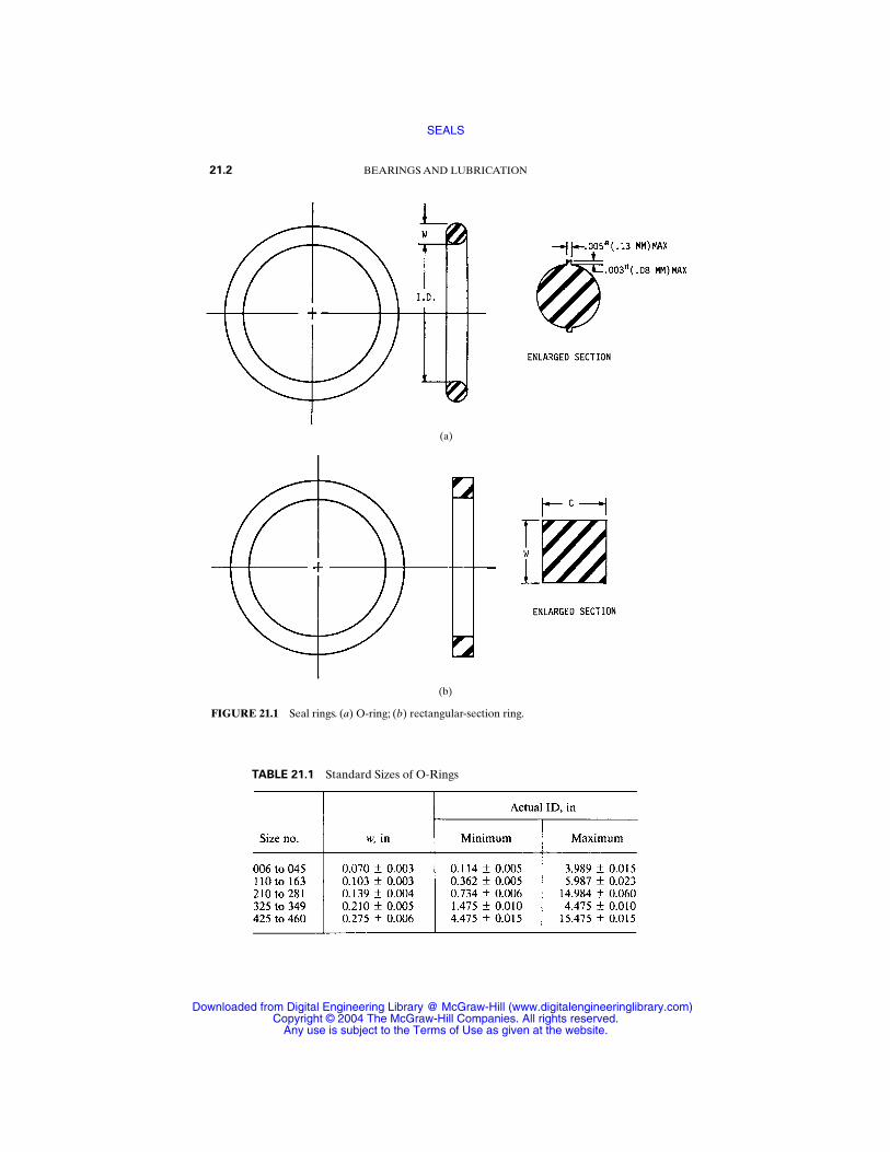
21.2 BEARINGS AND LUBRICATION
FIGURE 21.1 Seal rings. (a) O-ring; (b) rectangular-section ring.
(a)
(b)
TABLE 21.1 Standard Sizes of O-Rings
SEALS
Downloaded from Digital Engineering Library @ McGraw-Hill (www.digitalengineeringlibrary.com)Copyright © 2004 The McGraw-Hill Companies. All rights reserved.
Any use is subject to the Terms of Use as given at the website.
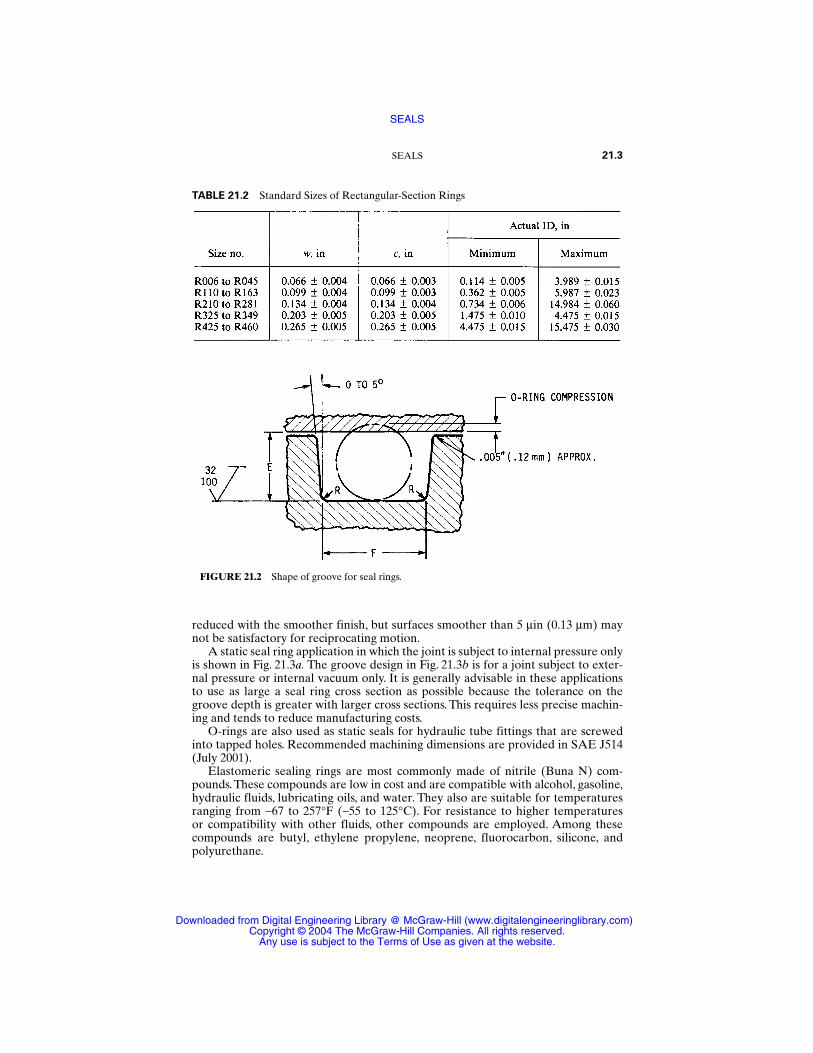
reduced with the smoother finish, but surfaces smoother than 5 µin (0.13 µm) maynot be satisfactory for reciprocating motion.
A static seal ring application in which the joint is subject to internal pressure onlyis shown in Fig. 21.3a. The groove design in Fig. 21.3b is for a joint subject to exter-nal pressure or internal vacuum only. It is generally advisable in these applicationsto use as large a seal ring cross section as possible because the tolerance on thegroove depth is greater with larger cross sections. This requires less precise machin-ing and tends to reduce manufacturing costs.
O-rings are also used as static seals for hydraulic tube fittings that are screwedinto tapped holes. Recommended machining dimensions are provided in SAE J514(July 2001).
Elastomeric sealing rings are most commonly made of nitrile (Buna N) com-pounds.These compounds are low in cost and are compatible with alcohol, gasoline,hydraulic fluids, lubricating oils, and water. They also are suitable for temperaturesranging from −67 to 257°F (−55 to 125°C). For resistance to higher temperatures or compatibility with other fluids, other compounds are employed. Among thesecompounds are butyl, ethylene propylene, neoprene, fluorocarbon, silicone, andpolyurethane.
SEALS 21.3
TABLE 21.2 Standard Sizes of Rectangular-Section Rings
FIGURE 21.2 Shape of groove for seal rings.
SEALS
Downloaded from Digital Engineering Library @ McGraw-Hill (www.digitalengineeringlibrary.com)Copyright © 2004 The McGraw-Hill Companies. All rights reserved.
Any use is subject to the Terms of Use as given at the website.
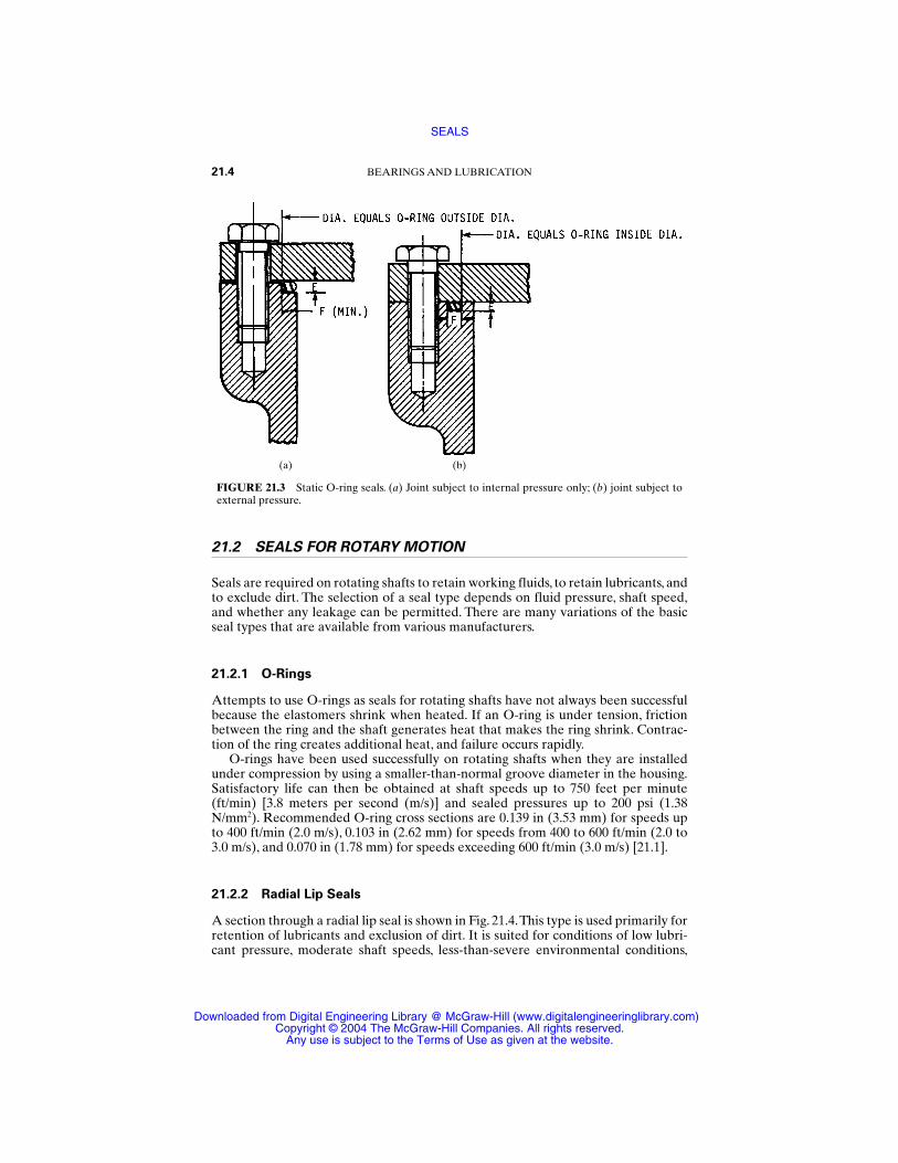
21.2 SEALS FOR ROTARY MOTION
Seals are required on rotating shafts to retain working fluids, to retain lubricants, andto exclude dirt. The selection of a seal type depends on fluid pressure, shaft speed,and whether any leakage can be permitted. There are many variations of the basicseal types that are available from various manufacturers.
21.2.1 O-Rings
Attempts to use O-rings as seals for rotating shafts have not always been successfulbecause the elastomers shrink when heated. If an O-ring is under tension, frictionbetween the ring and the shaft generates heat that makes the ring shrink. Contrac-tion of the ring creates additional heat, and failure occurs rapidly.
O-rings have been used successfully on rotating shafts when they are installedunder compression by using a smaller-than-normal groove diameter in the housing.Satisfactory life can then be obtained at shaft speeds up to 750 feet per minute(ft/min) [3.8 meters per second (m/s)] and sealed pressures up to 200 psi (1.38N/mm2). Recommended O-ring cross sections are 0.139 in (3.53 mm) for speeds upto 400 ft/min (2.0 m/s), 0.103 in (2.62 mm) for speeds from 400 to 600 ft/min (2.0 to3.0 m/s), and 0.070 in (1.78 mm) for speeds exceeding 600 ft/min (3.0 m/s) [21.1].
21.2.2 Radial Lip Seals
A section through a radial lip seal is shown in Fig. 21.4.This type is used primarily forretention of lubricants and exclusion of dirt. It is suited for conditions of low lubri-cant pressure, moderate shaft speeds, less-than-severe environmental conditions,
21.4 BEARINGS AND LUBRICATION
FIGURE 21.3 Static O-ring seals. (a) Joint subject to internal pressure only; (b) joint subject toexternal pressure.
(a) (b)
SEALS
Downloaded from Digital Engineering Library @ McGraw-Hill (www.digitalengineeringlibrary.com)Copyright © 2004 The McGraw-Hill Companies. All rights reserved.
Any use is subject to the Terms of Use as given at the website.
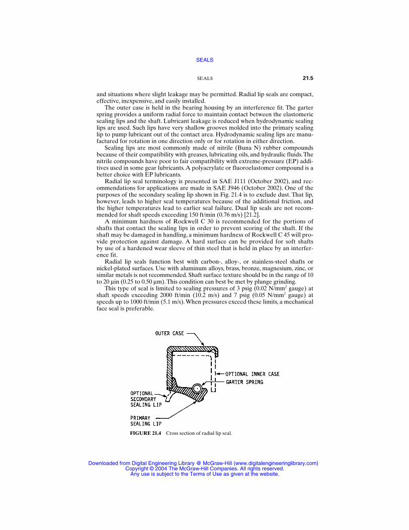
and situations where slight leakage may be permitted. Radial lip seals are compact,effective, inexpensive, and easily installed.
The outer case is held in the bearing housing by an interference fit. The garterspring provides a uniform radial force to maintain contact between the elastomericsealing lips and the shaft. Lubricant leakage is reduced when hydrodynamic sealinglips are used. Such lips have very shallow grooves molded into the primary sealinglip to pump lubricant out of the contact area. Hydrodynamic sealing lips are manu-factured for rotation in one direction only or for rotation in either direction.
Sealing lips are most commonly made of nitrile (Buna N) rubber compoundsbecause of their compatibility with greases, lubricating oils, and hydraulic fluids.Thenitrile compounds have poor to fair compatibility with extreme-pressure (EP) addi-tives used in some gear lubricants.A polyacrylate or fluoroelastomer compound is abetter choice with EP lubricants.
Radial lip seal terminology is presented in SAE J111 (October 2002), and rec-ommendations for applications are made in SAE J946 (October 2002). One of thepurposes of the secondary sealing lip shown in Fig. 21.4 is to exclude dust. That lip,however, leads to higher seal temperatures because of the additional friction, andthe higher temperatures lead to earlier seal failure. Dual lip seals are not recom-mended for shaft speeds exceeding 150 ft/min (0.76 m/s) [21.2].
A minimum hardness of Rockwell C 30 is recommended for the portions ofshafts that contact the sealing lips in order to prevent scoring of the shaft. If theshaft may be damaged in handling, a minimum hardness of Rockwell C 45 will pro-vide protection against damage. A hard surface can be provided for soft shafts by use of a hardened wear sleeve of thin steel that is held in place by an interfer-ence fit.
Radial lip seals function best with carbon-, alloy-, or stainless-steel shafts ornickel-plated surfaces. Use with aluminum alloys, brass, bronze, magnesium, zinc, orsimilar metals is not recommended. Shaft surface texture should be in the range of 10to 20 µin (0.25 to 0.50 µm). This condition can best be met by plunge grinding.
This type of seal is limited to sealing pressures of 3 psig (0.02 N/mm2 gauge) atshaft speeds exceeding 2000 ft/min (10.2 m/s) and 7 psig (0.05 N/mm2 gauge) atspeeds up to 1000 ft/min (5.1 m/s).When pressures exceed these limits, a mechanicalface seal is preferable.
SEALS 21.5
FIGURE 21.4 Cross section of radial lip seal.
SEALS
Downloaded from Digital Engineering Library @ McGraw-Hill (www.digitalengineeringlibrary.com)Copyright © 2004 The McGraw-Hill Companies. All rights reserved.
Any use is subject to the Terms of Use as given at the website.
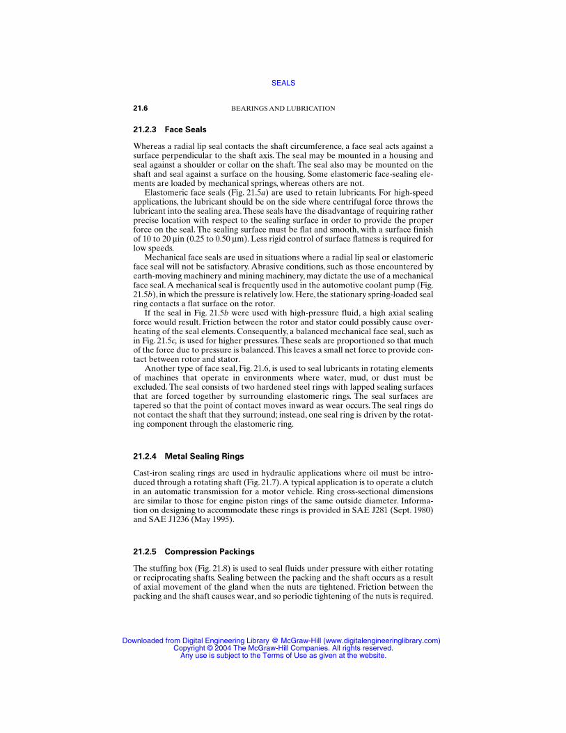
21.2.3 Face Seals
Whereas a radial lip seal contacts the shaft circumference, a face seal acts against asurface perpendicular to the shaft axis. The seal may be mounted in a housing andseal against a shoulder or collar on the shaft. The seal also may be mounted on theshaft and seal against a surface on the housing. Some elastomeric face-sealing ele-ments are loaded by mechanical springs, whereas others are not.
Elastomeric face seals (Fig. 21.5a) are used to retain lubricants. For high-speedapplications, the lubricant should be on the side where centrifugal force throws thelubricant into the sealing area.These seals have the disadvantage of requiring ratherprecise location with respect to the sealing surface in order to provide the properforce on the seal. The sealing surface must be flat and smooth, with a surface finishof 10 to 20 µin (0.25 to 0.50 µm). Less rigid control of surface flatness is required forlow speeds.
Mechanical face seals are used in situations where a radial lip seal or elastomericface seal will not be satisfactory. Abrasive conditions, such as those encountered byearth-moving machinery and mining machinery, may dictate the use of a mechanicalface seal.A mechanical seal is frequently used in the automotive coolant pump (Fig.21.5b), in which the pressure is relatively low. Here, the stationary spring-loaded sealring contacts a flat surface on the rotor.
If the seal in Fig. 21.5b were used with high-pressure fluid, a high axial sealingforce would result. Friction between the rotor and stator could possibly cause over-heating of the seal elements. Consequently, a balanced mechanical face seal, such asin Fig. 21.5c, is used for higher pressures. These seals are proportioned so that muchof the force due to pressure is balanced.This leaves a small net force to provide con-tact between rotor and stator.
Another type of face seal, Fig. 21.6, is used to seal lubricants in rotating elementsof machines that operate in environments where water, mud, or dust must beexcluded. The seal consists of two hardened steel rings with lapped sealing surfacesthat are forced together by surrounding elastomeric rings. The seal surfaces aretapered so that the point of contact moves inward as wear occurs. The seal rings donot contact the shaft that they surround; instead, one seal ring is driven by the rotat-ing component through the elastomeric ring.
21.2.4 Metal Sealing Rings
Cast-iron sealing rings are used in hydraulic applications where oil must be intro-duced through a rotating shaft (Fig. 21.7).A typical application is to operate a clutchin an automatic transmission for a motor vehicle. Ring cross-sectional dimensionsare similar to those for engine piston rings of the same outside diameter. Informa-tion on designing to accommodate these rings is provided in SAE J281 (Sept. 1980)and SAE J1236 (May 1995).
21.2.5 Compression Packings
The stuffing box (Fig. 21.8) is used to seal fluids under pressure with either rotatingor reciprocating shafts. Sealing between the packing and the shaft occurs as a resultof axial movement of the gland when the nuts are tightened. Friction between thepacking and the shaft causes wear, and so periodic tightening of the nuts is required.
21.6 BEARINGS AND LUBRICATION
SEALS
Downloaded from Digital Engineering Library @ McGraw-Hill (www.digitalengineeringlibrary.com)Copyright © 2004 The McGraw-Hill Companies. All rights reserved.
Any use is subject to the Terms of Use as given at the website.
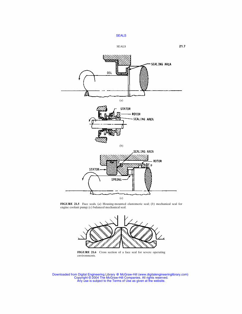
SEALS 21.7
FIGURE 21.5 Face seals. (a) Housing-mounted elastomeric seal; (b) mechanical seal forengine coolant pump; (c) balanced mechanical seal.
(a)
(b)
(c)
FIGURE 21.6 Cross section of a face seal for severe operatingenvironments.
SEALS
Downloaded from Digital Engineering Library @ McGraw-Hill (www.digitalengineeringlibrary.com)Copyright © 2004 The McGraw-Hill Companies. All rights reserved.
Any use is subject to the Terms of Use as given at the website.
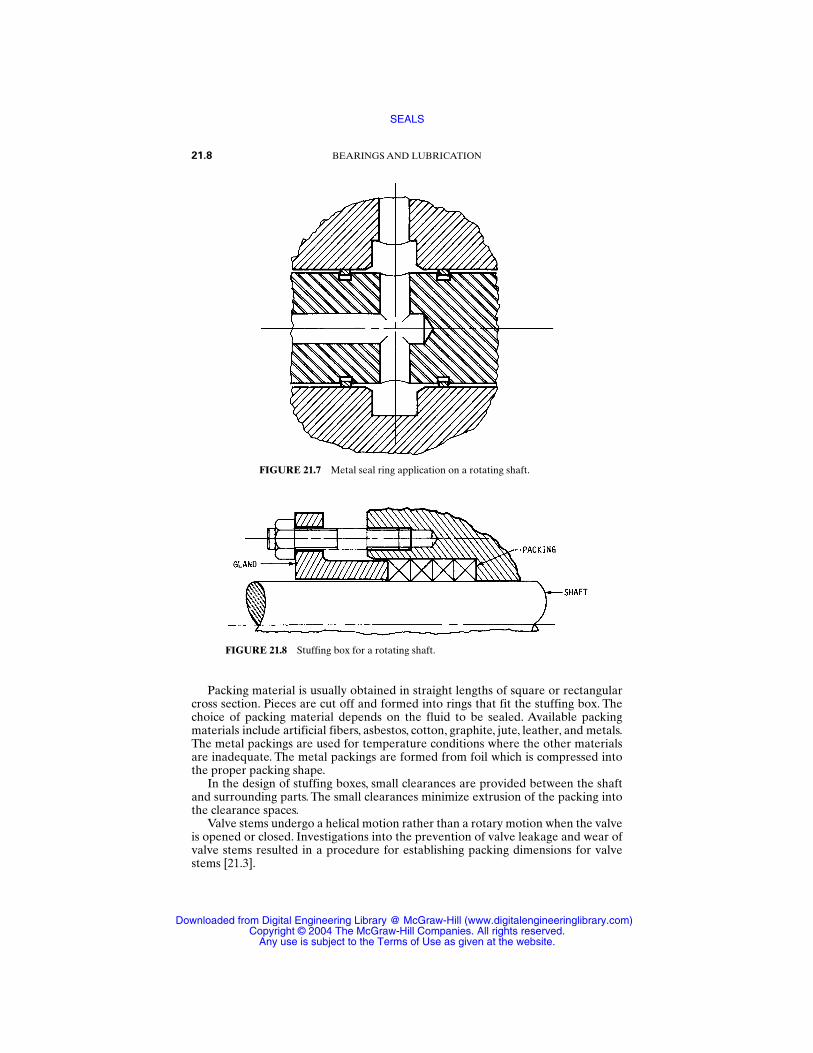
Packing material is usually obtained in straight lengths of square or rectangularcross section. Pieces are cut off and formed into rings that fit the stuffing box. Thechoice of packing material depends on the fluid to be sealed. Available packingmaterials include artificial fibers, asbestos, cotton, graphite, jute, leather, and metals.The metal packings are used for temperature conditions where the other materialsare inadequate. The metal packings are formed from foil which is compressed intothe proper packing shape.
In the design of stuffing boxes, small clearances are provided between the shaftand surrounding parts. The small clearances minimize extrusion of the packing intothe clearance spaces.
Valve stems undergo a helical motion rather than a rotary motion when the valveis opened or closed. Investigations into the prevention of valve leakage and wear ofvalve stems resulted in a procedure for establishing packing dimensions for valvestems [21.3].
21.8 BEARINGS AND LUBRICATION
FIGURE 21.7 Metal seal ring application on a rotating shaft.
FIGURE 21.8 Stuffing box for a rotating shaft.
SEALS
Downloaded from Digital Engineering Library @ McGraw-Hill (www.digitalengineeringlibrary.com)Copyright © 2004 The McGraw-Hill Companies. All rights reserved.
Any use is subject to the Terms of Use as given at the website.
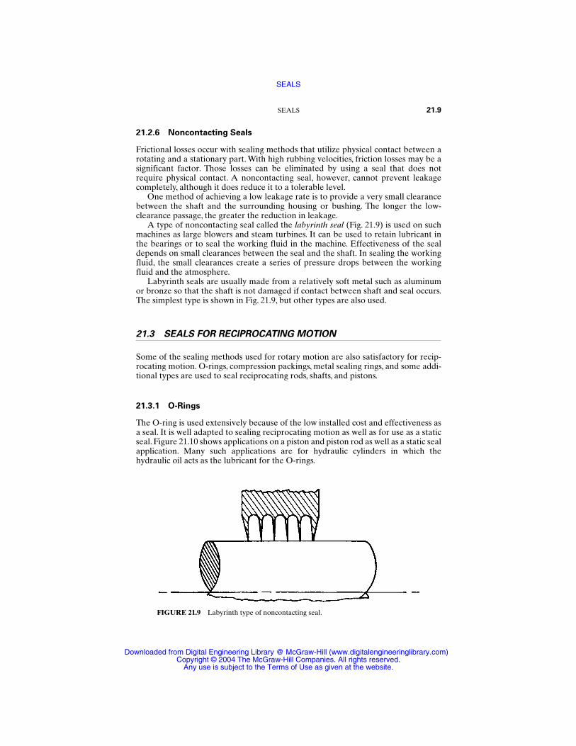
21.2.6 Noncontacting Seals
Frictional losses occur with sealing methods that utilize physical contact between arotating and a stationary part. With high rubbing velocities, friction losses may be asignificant factor. Those losses can be eliminated by using a seal that does notrequire physical contact. A noncontacting seal, however, cannot prevent leakagecompletely, although it does reduce it to a tolerable level.
One method of achieving a low leakage rate is to provide a very small clearancebetween the shaft and the surrounding housing or bushing. The longer the low-clearance passage, the greater the reduction in leakage.
A type of noncontacting seal called the labyrinth seal (Fig. 21.9) is used on suchmachines as large blowers and steam turbines. It can be used to retain lubricant inthe bearings or to seal the working fluid in the machine. Effectiveness of the sealdepends on small clearances between the seal and the shaft. In sealing the workingfluid, the small clearances create a series of pressure drops between the workingfluid and the atmosphere.
Labyrinth seals are usually made from a relatively soft metal such as aluminumor bronze so that the shaft is not damaged if contact between shaft and seal occurs.The simplest type is shown in Fig. 21.9, but other types are also used.
21.3 SEALS FOR RECIPROCATING MOTION
Some of the sealing methods used for rotary motion are also satisfactory for recip-rocating motion. O-rings, compression packings, metal sealing rings, and some addi-tional types are used to seal reciprocating rods, shafts, and pistons.
21.3.1 O-Rings
The O-ring is used extensively because of the low installed cost and effectiveness asa seal. It is well adapted to sealing reciprocating motion as well as for use as a staticseal. Figure 21.10 shows applications on a piston and piston rod as well as a static sealapplication. Many such applications are for hydraulic cylinders in which thehydraulic oil acts as the lubricant for the O-rings.
SEALS 21.9
FIGURE 21.9 Labyrinth type of noncontacting seal.
SEALS
Downloaded from Digital Engineering Library @ McGraw-Hill (www.digitalengineeringlibrary.com)Copyright © 2004 The McGraw-Hill Companies. All rights reserved.
Any use is subject to the Terms of Use as given at the website.
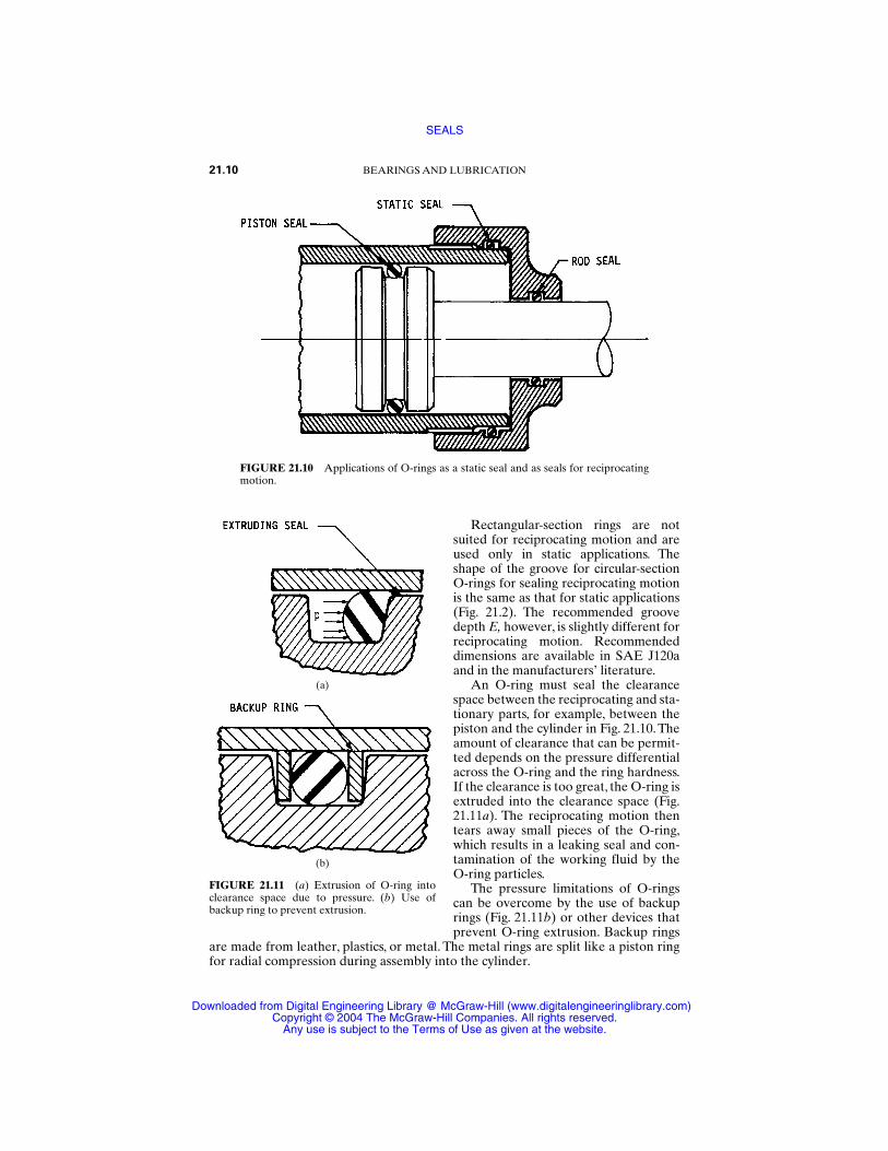
Rectangular-section rings are notsuited for reciprocating motion and areused only in static applications. Theshape of the groove for circular-sectionO-rings for sealing reciprocating motionis the same as that for static applications(Fig. 21.2). The recommended groovedepth E, however, is slightly different forreciprocating motion. Recommendeddimensions are available in SAE J120aand in the manufacturers’ literature.
An O-ring must seal the clearancespace between the reciprocating and sta-tionary parts, for example, between thepiston and the cylinder in Fig. 21.10. Theamount of clearance that can be permit-ted depends on the pressure differentialacross the O-ring and the ring hardness.If the clearance is too great, the O-ring isextruded into the clearance space (Fig.21.11a). The reciprocating motion thentears away small pieces of the O-ring,which results in a leaking seal and con-tamination of the working fluid by theO-ring particles.
The pressure limitations of O-ringscan be overcome by the use of backuprings (Fig. 21.11b) or other devices thatprevent O-ring extrusion. Backup rings
are made from leather, plastics, or metal. The metal rings are split like a piston ringfor radial compression during assembly into the cylinder.
21.10 BEARINGS AND LUBRICATION
FIGURE 21.10 Applications of O-rings as a static seal and as seals for reciprocatingmotion.
FIGURE 21.11 (a) Extrusion of O-ring intoclearance space due to pressure. (b) Use ofbackup ring to prevent extrusion.
(a)
(b)
SEALS
Downloaded from Digital Engineering Library @ McGraw-Hill (www.digitalengineeringlibrary.com)Copyright © 2004 The McGraw-Hill Companies. All rights reserved.
Any use is subject to the Terms of Use as given at the website.
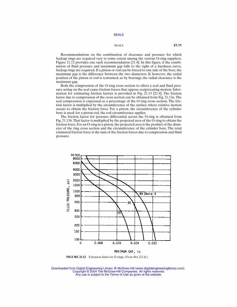
Recommendations on the combination of clearance and pressure for whichbackup rings are required vary to some extent among the various O-ring suppliers.Figure 21.12 provides one such recommendation [21.4]. In this figure, if the combi-nation of fluid pressure and maximum gap falls to the right of a hardness curve,backup rings are required. If a piston or rod can be forced to one side of the bore, themaximum gap is the difference between the two diameters. If, however, the radialposition of the piston or rod is restrained, as by bearings, the radial clearance is themaximum gap.
Both the compression of the O-ring cross section to effect a seal and fluid pres-sure acting on the seal cause friction forces that oppose reciprocating motion. Infor-mation for estimating friction factors is provided in Fig. 21.13 [21.4]. The frictionfactor due to compression of the cross section can be obtained from Fig. 21.13a. Theseal compression is expressed as a percentage of the O-ring cross section. The fric-tion factor is multiplied by the circumference of the surface where relative motionoccurs to obtain the friction force. For a piston, the circumference of the cylinderbore is used; for a piston rod, the rod circumference applies.
The friction factor for pressure differential across the O-ring is obtained fromFig. 21.13b. That factor is multiplied by the projected area of the O-ring to obtain thefriction force. For an O-ring in a piston, the projected area is the product of the diam-eter of the ring cross section and the circumference of the cylinder bore. The totalestimated friction force is the sum of the friction forces due to compression and fluidpressure.
SEALS 21.11
FIGURE 21.12 Extrusion limits for O-rings. (From Ref. [21.4].)
SEALS
Downloaded from Digital Engineering Library @ McGraw-Hill (www.digitalengineeringlibrary.com)Copyright © 2004 The McGraw-Hill Companies. All rights reserved.
Any use is subject to the Terms of Use as given at the website.
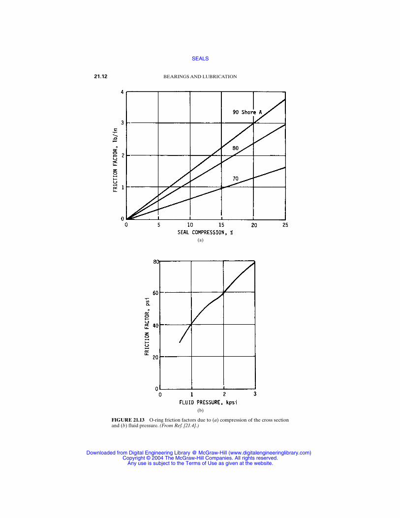
21.12 BEARINGS AND LUBRICATION
FIGURE 21.13 O-ring friction factors due to (a) compression of the cross sectionand (b) fluid pressure. (From Ref. [21.4].)
(a)
(b)
SEALS
Downloaded from Digital Engineering Library @ McGraw-Hill (www.digitalengineeringlibrary.com)Copyright © 2004 The McGraw-Hill Companies. All rights reserved.
Any use is subject to the Terms of Use as given at the website.
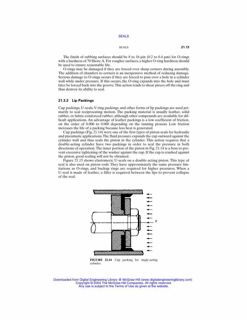
The finish of rubbing surfaces should be 8 to 16 µin (0.2 to 0.4 µm) for O-ringswith a hardness of 70 Shore A. For rougher surfaces, a higher O-ring hardness shouldbe used to ensure reasonable life.
O-rings may be damaged if they are forced over sharp corners during assembly.The addition of chamfers to corners is an inexpensive method of reducing damage.Serious damage to O-rings occurs if they are forced to pass over a hole in a cylinderwall while under pressure. If this occurs, the O-ring expands into the hole and mustlater be forced back into the groove.This action tends to shear pieces off the ring andthus destroy its ability to seal.
21.3.2 Lip Packings
Cup packings, U-seals, V-ring packings, and other forms of lip packings are used pri-marily to seal reciprocating motion. The packing material is usually leather, solidrubber, or fabric-reinforced rubber, although other compounds are available for dif-ficult applications. An advantage of leather packings is a low coefficient of friction,on the order of 0.006 to 0.008 depending on the tanning process. Low frictionincreases the life of a packing because less heat is generated.
Cup packings (Fig. 21.14) were one of the first types of piston seals for hydraulicand pneumatic applications.The fluid pressure expands the cup outward against thecylinder wall and thus seals the piston in the cylinder. This action requires that adouble-acting cylinder have two packings in order to seal the pressure in bothdirections of operation.The inner portion of the piston in Fig. 21.14 is a boss to pre-vent excessive tightening of the washer against the cup. If the cup is crushed againstthe piston, good sealing will not be obtained.
Figure 21.15 shows elastomeric U-seals on a double-acting piston. This type ofseal is also used on piston rods. They have approximately the same pressure lim-itations as O-rings, and backup rings are required for higher pressures. When a U-seal is made of leather, a filler is required between the lips to prevent collapseof the seal.
SEALS 21.13
FIGURE 21.14 Cup packing for single-actingcylinder.
SEALS
Downloaded from Digital Engineering Library @ McGraw-Hill (www.digitalengineeringlibrary.com)Copyright © 2004 The McGraw-Hill Companies. All rights reserved.
Any use is subject to the Terms of Use as given at the website.
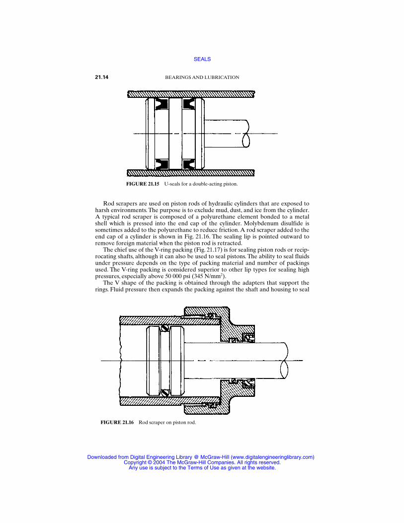
Rod scrapers are used on piston rods of hydraulic cylinders that are exposed toharsh environments. The purpose is to exclude mud, dust, and ice from the cylinder.A typical rod scraper is composed of a polyurethane element bonded to a metalshell which is pressed into the end cap of the cylinder. Molybdenum disulfide issometimes added to the polyurethane to reduce friction. A rod scraper added to theend cap of a cylinder is shown in Fig. 21.16. The sealing lip is pointed outward toremove foreign material when the piston rod is retracted.
The chief use of the V-ring packing (Fig. 21.17) is for sealing piston rods or recip-rocating shafts, although it can also be used to seal pistons. The ability to seal fluidsunder pressure depends on the type of packing material and number of packingsused. The V-ring packing is considered superior to other lip types for sealing highpressures, especially above 50 000 psi (345 N/mm2).
The V shape of the packing is obtained through the adapters that support therings. Fluid pressure then expands the packing against the shaft and housing to seal
21.14 BEARINGS AND LUBRICATION
FIGURE 21.15 U-seals for a double-acting piston.
FIGURE 21.16 Rod scraper on piston rod.
SEALS
Downloaded from Digital Engineering Library @ McGraw-Hill (www.digitalengineeringlibrary.com)Copyright © 2004 The McGraw-Hill Companies. All rights reserved.
Any use is subject to the Terms of Use as given at the website.
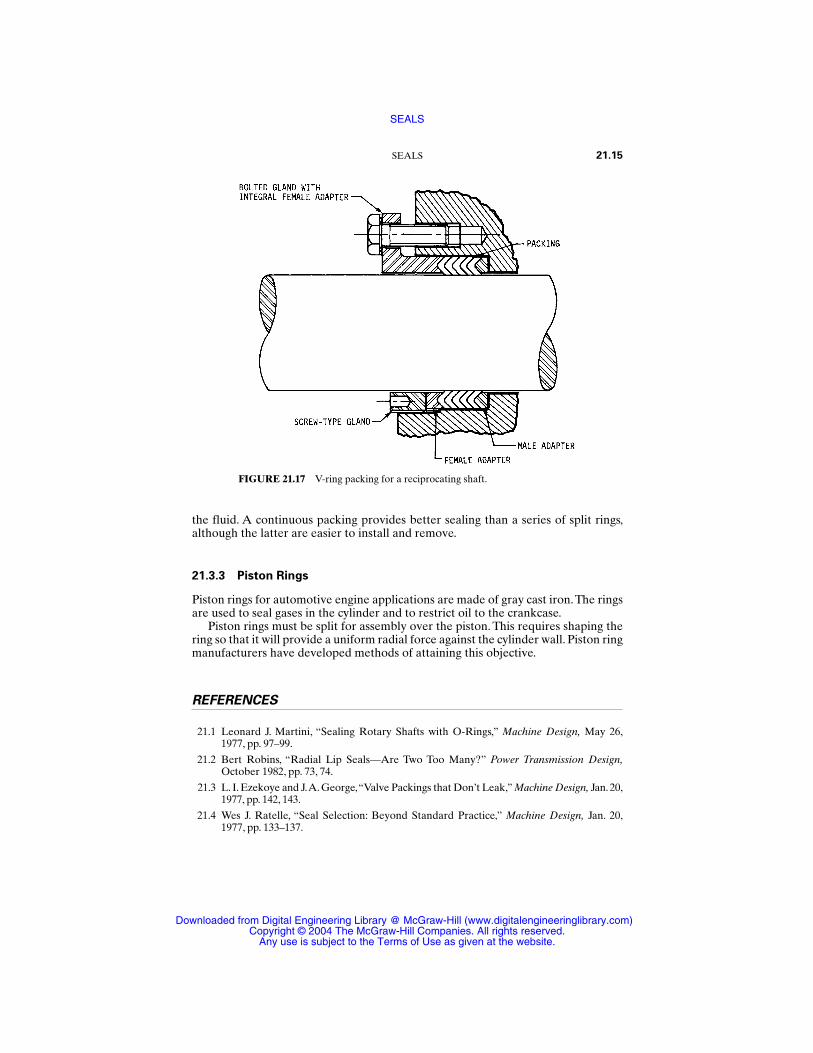
the fluid. A continuous packing provides better sealing than a series of split rings,although the latter are easier to install and remove.
21.3.3 Piston Rings
Piston rings for automotive engine applications are made of gray cast iron.The ringsare used to seal gases in the cylinder and to restrict oil to the crankcase.
Piston rings must be split for assembly over the piston. This requires shaping thering so that it will provide a uniform radial force against the cylinder wall. Piston ringmanufacturers have developed methods of attaining this objective.
REFERENCES
21.1 Leonard J. Martini, “Sealing Rotary Shafts with O-Rings,” Machine Design, May 26,1977, pp. 97–99.
21.2 Bert Robins, “Radial Lip Seals—Are Two Too Many?” Power Transmission Design,October 1982, pp. 73, 74.
21.3 L. I. Ezekoye and J.A. George,“Valve Packings that Don’t Leak,” Machine Design, Jan. 20,1977, pp. 142, 143.
21.4 Wes J. Ratelle, “Seal Selection: Beyond Standard Practice,” Machine Design, Jan. 20,1977, pp. 133–137.
SEALS 21.15
FIGURE 21.17 V-ring packing for a reciprocating shaft.
SEALS
Downloaded from Digital Engineering Library @ McGraw-Hill (www.digitalengineeringlibrary.com)Copyright © 2004 The McGraw-Hill Companies. All rights reserved.
Any use is subject to the Terms of Use as given at the website.

SEALS
Downloaded from Digital Engineering Library @ McGraw-Hill (www.digitalengineeringlibrary.com)Copyright © 2004 The McGraw-Hill Companies. All rights reserved.
Any use is subject to the Terms of Use as given at the website.

P • A • R • T • 6
FASTENING, JOINING,AND CONNECTING
Source: STANDARD HANDBOOK OF MACHINE DESIGN
Downloaded from Digital Engineering Library @ McGraw-Hill (www.digitalengineeringlibrary.com)Copyright © 2004 The McGraw-Hill Companies. All rights reserved.
Any use is subject to the Terms of Use as given at the website.

FASTENING, JOINING, AND CONNECTING
Downloaded from Digital Engineering Library @ McGraw-Hill (www.digitalengineeringlibrary.com)Copyright © 2004 The McGraw-Hill Companies. All rights reserved.
Any use is subject to the Terms of Use as given at the website.

CHAPTER 22BOLTED AND RIVETED
JOINTS
John H. BickfordVice President, Manager of the Power-Dyne Division, Retired
Raymond Engineering Inc.Middletown, Connecticut
22.1 SHEAR LOADING OF JOINTS / 22.6
22.2 ECCENTRIC LOADS ON SHEAR JOINTS / 22.13
22.3 TENSION-LOADED JOINTS: PRELOADING OF BOLTS / 22.18
22.4 BOLT TORQUE REQUIREMENTS / 22.31
22.5 FATIGUE LOADING OF BOLTED AND RIVETED JOINTS / 22.31
22.6 PROGRAMMING SUGGESTIONS FOR JOINTS LOADED IN TENSION / 22.38
REFERENCES / 22.40
SYMBOLS AND UNITS
A Cross-sectional area, in2 (mm2)AB Cross-sectional area of the body of a bolt, in2 (mm2)Ar Cross-sectional area of the body of the rivet, in2 (mm2)AS Cross-sectional area of the tensile stress area of the threaded
portion of a bolt, in2 (mm2)A1, A2, A3, etc. Cross-sectional areas of individual fasteners, in2 (mm2)b Number of shear planes which pass through the fastener; and/or
the number of slip surfaces in a shear jointd Nominal diameter of the bolt, in (mm)E Modulus of elasticity, psi (MPa)F Force, lb (kN)FB Tension in a bolt, lb (kN)Fb Primary shear force on a bolt, lb (kN)FB(max) Maximum anticipated tension in the bolt, lb (kN)FBY Tension in a bolt at yield, lb (kN)FC Clamping force on the joint, lb (kN)FC(min) Minimum acceptable clamping force on a joint, lb (kN)FJ(min) Minimum anticipated clamping force on the joint, lb (kN)
22.3
Source: STANDARD HANDBOOK OF MACHINE DESIGN
Downloaded from Digital Engineering Library @ McGraw-Hill (www.digitalengineeringlibrary.com)Copyright © 2004 The McGraw-Hill Companies. All rights reserved.
Any use is subject to the Terms of Use as given at the website.

Fn Reaction moment force seen by the nth bolt in an eccentricallyloaded shear joint, lb (kN)
FPA Average preload in a group of bolts, lb (kN)FP(max) Maximum anticipated initial preload in a bolt, lb (kN)FP(min) Minimum anticipated initial preload in a bolt, lb (kN)FPT Target preload, lb (kN)FTR Maximum external transverse load on the joint, per bolt, lb
(kN)
Fr External shear load on the rivet, lb (kN)
FT(max) Maximum acceptable tension in a bolt, lb (kN)
FX External tension load on a joint, lb (kN)
F1, F2, F3, etc. Secondary shear or reaction moment forces seen by individualbolts in an eccentric joint, lb (kN)
H Distance between the centerline of the bolt holes nearest to theedge of a joint or splice plate and that edge, in (mm)
kB Stiffness of a bolt or rivet, lb/in (kN/mm)
kG Stiffness of a gasket, lb/in (kN/mm)
kJ Stiffness of the joint members, lb/in (kN/mm)
kT Stiffness of gasketed joint, lb/in (kN/mm)
K Nut factor
lG Grip length of the fasteners, in (mm)
L Distance between the bolt and the nearest edge of the con-nected part, or to the nearest edge of the next bolt hole, mea-sured in the direction of the force on the joint, in (mm)
LB Effective length of the body of a bolt (the length of body in thegrip plus one-half the thickness of the head, for example), in(mm)
LS Effective length of the threaded portion of a bolt [the length ofthe threads within the grip plus one-half the thickness of thenut(s), for example], in (mm)
m Number of fasteners in the joint
M Moment exerted on a shear joint by an external force, lb ⋅ in(N ⋅ m)
n Number of threads per inch
N Number of cycles achieved in fatigue life test
P Pitch of the threads, in (mm)
PS Scatter in preload anticipated from bolting tool used for assem-bly (expressed as a decimal)
PZ Percentage loss (expressed as a decimal) in initial preload as aresult of short-term relaxation and/or elastic interactions
r Radial distance from the centroid of a group of fasteners to afastener, in (mm)
rn Radial distance to the nth fastener, in (mm)
22.4 FASTENING, JOINING, AND CONNECTING
BOLTED AND RIVETED JOINTS
Downloaded from Digital Engineering Library @ McGraw-Hill (www.digitalengineeringlibrary.com)Copyright © 2004 The McGraw-Hill Companies. All rights reserved.
Any use is subject to the Terms of Use as given at the website.

rs Bolt slenderness ratio (lG/d)r1, r2, r3, etc. Radial distance of individual fasteners, in (mm)RJB Stiffness ratio (kJ/kB)RS Slip resistance of a friction-type joint, lb (kN)S Ratio of the ultimate shear strength of the bolt material to its
ultimate tensile strengthSu Minimum ultimate tensile strength, psi (MPa)SYB Yield strength of the bolt, psi (MPa)t Thickness of a joint or a splice plate, in (mm)tJ Total thickness of a joint, in (mm)T Torque, lb ⋅ in (N ⋅ m)W Width of a joint plate, in (mm)x Coordinate distance, in (mm)x Coordinate distance to the centroid of a bolt group, in (mm)x1, x2, x3, etc. x coordinates for individual fasteners, in (mm)y Coordinate distance, in (mm)y Coordinate distance to the centroid of a bolt group, in (mm)y1, y2, y3, etc. y coordinates for individual fasteners, in (mm)∆ Incremental change or variationλ Ratio of shear stress in a bolt to the ultimate tensile strengthµS Slip coefficient of a friction-type jointσ Stress, psi (MPa)σB Bearing stress, psi (MPa)σ(max) Maximum tensile stress imposed during fatigue tests, psi (MPa)σT Allowable tensile stress, psi (MPa)σT (max) Maximum acceptable tensile stress in a bolt, psi (MPa)ç2 Statistical variance (standard deviation squared)çO
2 Statistical variance of the tension errors created by operatorvariables
çT2 Statistical variance of the tension errors created by tool vari-
ablesτ Shear stress, psi (MPa)τA Allowable shear stress, psi (MPa)τB Shear stress in a bolt, psi (MPa)φ Ratio of tensile stress in a bolt to the ultimate tensile strength
Joints are an extremely important part of any structure. Whether held together bybolts or rivets or weldments or adhesives or something else, joints make complexstructures and machines possible. Bolted joints, at least, also make disassembly andreassembly possible.And many joints are critical elements of the structure, the thingmost likely to fail. Because of this, it is important for the designer to understandjoints. In this chapter we will deal specifically with bolted and riveted joints, startingwith a discussion of joints loaded in shear (with the applied loads at right angles to
BOLTED AND RIVETED JOINTS 22.5
BOLTED AND RIVETED JOINTS
Downloaded from Digital Engineering Library @ McGraw-Hill (www.digitalengineeringlibrary.com)Copyright © 2004 The McGraw-Hill Companies. All rights reserved.
Any use is subject to the Terms of Use as given at the website.
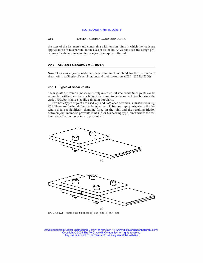
the axes of the fasteners) and continuing with tension joints in which the loads areapplied more or less parallel to the axes of fasteners.As we shall see, the design pro-cedures for shear joints and tension joints are quite different.
22.1 SHEAR LOADING OF JOINTS
Now let us look at joints loaded in shear. I am much indebted, for the discussion ofshear joints, to Shigley, Fisher, Higdon, and their coauthors ([22.1], [22.2], [22.3]).
22.1.1 Types of Shear Joints
Shear joints are found almost exclusively in structural steel work. Such joints can beassembled with either rivets or bolts. Rivets used to be the only choice, but since theearly 1950s, bolts have steadily gained in popularity.
Two basic types of joint are used, lap and butt, each of which is illustrated in Fig.22.1. These are further defined as being either (1) friction-type joints, where the fas-teners create a significant clamping force on the joint and the resulting frictionbetween joint members prevents joint slip, or (2) bearing-type joints, where the fas-teners, in effect, act as points to prevent slip.
22.6 FASTENING, JOINING, AND CONNECTING
FIGURE 22.1 Joints loaded in shear. (a) Lap joint; (b) butt joint.
(a)
(b)
BOLTED AND RIVETED JOINTS
Downloaded from Digital Engineering Library @ McGraw-Hill (www.digitalengineeringlibrary.com)Copyright © 2004 The McGraw-Hill Companies. All rights reserved.
Any use is subject to the Terms of Use as given at the website.
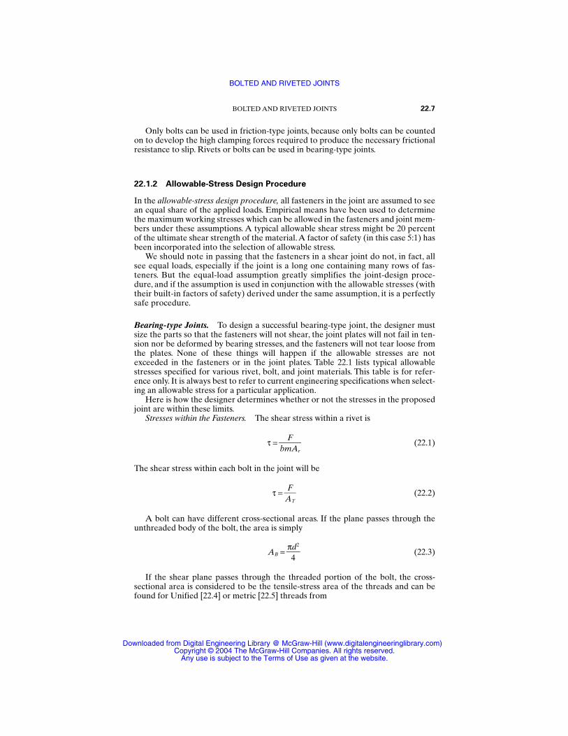
Only bolts can be used in friction-type joints, because only bolts can be countedon to develop the high clamping forces required to produce the necessary frictionalresistance to slip. Rivets or bolts can be used in bearing-type joints.
22.1.2 Allowable-Stress Design Procedure
In the allowable-stress design procedure, all fasteners in the joint are assumed to seean equal share of the applied loads. Empirical means have been used to determinethe maximum working stresses which can be allowed in the fasteners and joint mem-bers under these assumptions. A typical allowable shear stress might be 20 percentof the ultimate shear strength of the material.A factor of safety (in this case 5:1) hasbeen incorporated into the selection of allowable stress.
We should note in passing that the fasteners in a shear joint do not, in fact, allsee equal loads, especially if the joint is a long one containing many rows of fas-teners. But the equal-load assumption greatly simplifies the joint-design proce-dure, and if the assumption is used in conjunction with the allowable stresses (withtheir built-in factors of safety) derived under the same assumption, it is a perfectlysafe procedure.
Bearing-type Joints. To design a successful bearing-type joint, the designer mustsize the parts so that the fasteners will not shear, the joint plates will not fail in ten-sion nor be deformed by bearing stresses, and the fasteners will not tear loose fromthe plates. None of these things will happen if the allowable stresses are notexceeded in the fasteners or in the joint plates. Table 22.1 lists typical allowablestresses specified for various rivet, bolt, and joint materials. This table is for refer-ence only. It is always best to refer to current engineering specifications when select-ing an allowable stress for a particular application.
Here is how the designer determines whether or not the stresses in the proposedjoint are within these limits.
Stresses within the Fasteners. The shear stress within a rivet is
τ = (22.1)
The shear stress within each bolt in the joint will be
τ = (22.2)
A bolt can have different cross-sectional areas. If the plane passes through theunthreaded body of the bolt, the area is simply
AB = (22.3)
If the shear plane passes through the threaded portion of the bolt, the cross-sectional area is considered to be the tensile-stress area of the threads and can befound for Unified [22.4] or metric [22.5] threads from
πd2
4
FAT
FbmAr
BOLTED AND RIVETED JOINTS 22.7
BOLTED AND RIVETED JOINTS
Downloaded from Digital Engineering Library @ McGraw-Hill (www.digitalengineeringlibrary.com)Copyright © 2004 The McGraw-Hill Companies. All rights reserved.
Any use is subject to the Terms of Use as given at the website.
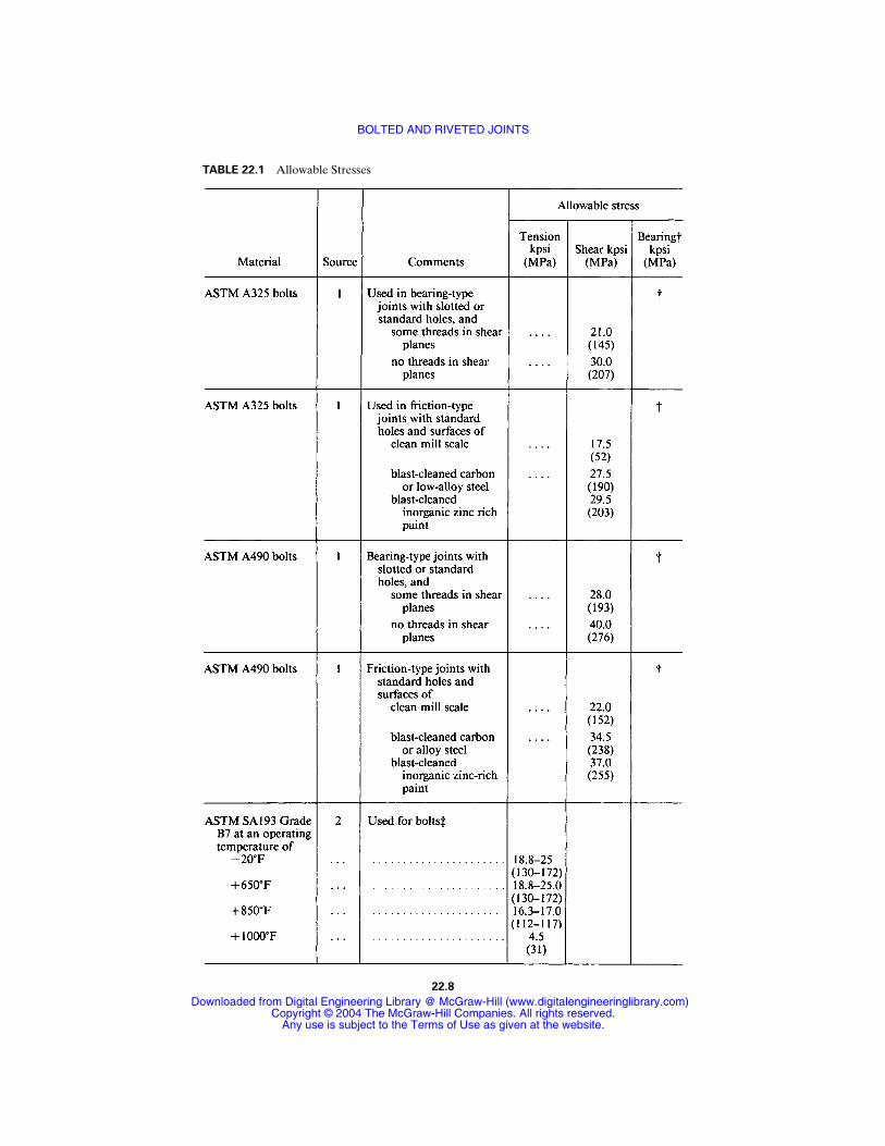
TABLE 22.1 Allowable Stresses
22.8
BOLTED AND RIVETED JOINTS
Downloaded from Digital Engineering Library @ McGraw-Hill (www.digitalengineeringlibrary.com)Copyright © 2004 The McGraw-Hill Companies. All rights reserved.
Any use is subject to the Terms of Use as given at the website.
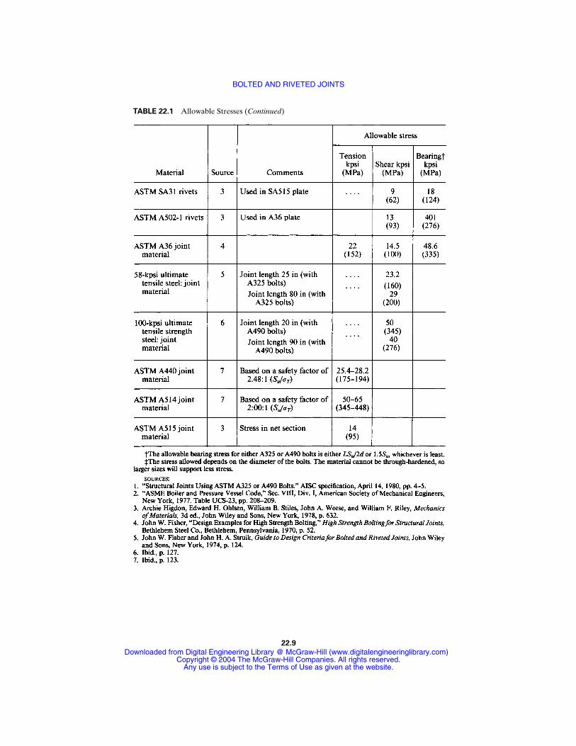
TABLE 22.1 Allowable Stresses (Continued)
22.9
BOLTED AND RIVETED JOINTS
Downloaded from Digital Engineering Library @ McGraw-Hill (www.digitalengineeringlibrary.com)Copyright © 2004 The McGraw-Hill Companies. All rights reserved.
Any use is subject to the Terms of Use as given at the website.
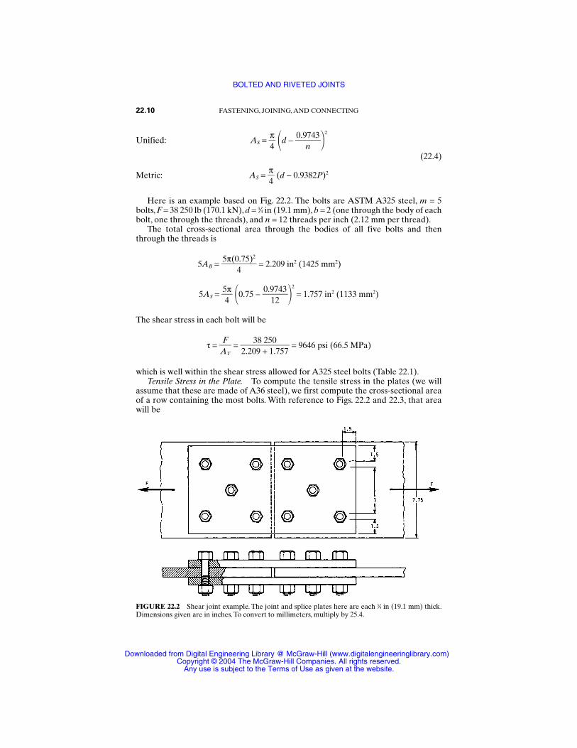
Unified: AS = π4
d − 0.9
n743
2
(22.4)
Metric: AS = π4
(d − 0.9382P)2
Here is an example based on Fig. 22.2. The bolts are ASTM A325 steel, m = 5bolts, F = 38 250 lb (170.1 kN), d = 3⁄4 in (19.1 mm), b = 2 (one through the body of eachbolt, one through the threads), and n = 12 threads per inch (2.12 mm per thread).
The total cross-sectional area through the bodies of all five bolts and thenthrough the threads is
5AB = = 2.209 in2 (1425 mm2)
5AS = 54π 0.75 −
0.917243
2
= 1.757 in2 (1133 mm2)
The shear stress in each bolt will be
τ = AF
T =
2.20398
+25
10.757
= 9646 psi (66.5 MPa)
which is well within the shear stress allowed for A325 steel bolts (Table 22.1).Tensile Stress in the Plate. To compute the tensile stress in the plates (we will
assume that these are made of A36 steel), we first compute the cross-sectional areaof a row containing the most bolts. With reference to Figs. 22.2 and 22.3, that areawill be
5π(0.75)2
4
22.10 FASTENING, JOINING, AND CONNECTING
FIGURE 22.2 Shear joint example. The joint and splice plates here are each 3⁄4 in (19.1 mm) thick.Dimensions given are in inches. To convert to millimeters, multiply by 25.4.
BOLTED AND RIVETED JOINTS
Downloaded from Digital Engineering Library @ McGraw-Hill (www.digitalengineeringlibrary.com)Copyright © 2004 The McGraw-Hill Companies. All rights reserved.
Any use is subject to the Terms of Use as given at the website.
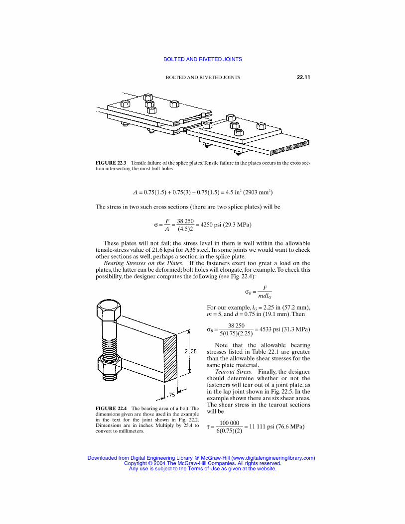
A = 0.75(1.5) + 0.75(3) + 0.75(1.5) = 4.5 in2 (2903 mm2)
The stress in two such cross sections (there are two splice plates) will be
σ = AF
= 3(84.
255)20
= 4250 psi (29.3 MPa)
These plates will not fail; the stress level in them is well within the allowable tensile-stress value of 21.6 kpsi for A36 steel. In some joints we would want to checkother sections as well, perhaps a section in the splice plate.
Bearing Stresses on the Plates. If the fasteners exert too great a load on theplates, the latter can be deformed; bolt holes will elongate, for example.To check thispossibility, the designer computes the following (see Fig. 22.4):
σB = m
FdlG
For our example, lG = 2.25 in (57.2 mm),m = 5, and d = 0.75 in (19.1 mm). Then
σB =5(0.
3785)2(520.25)
= 4533 psi (31.3 MPa)
Note that the allowable bearingstresses listed in Table 22.1 are greaterthan the allowable shear stresses for thesame plate material.
Tearout Stress. Finally, the designershould determine whether or not thefasteners will tear out of a joint plate, asin the lap joint shown in Fig. 22.5. In theexample shown there are six shear areas.The shear stress in the tearout sectionswill be
τ = 6(
100.075
0)0(02)
= 11 111 psi (76.6 MPa)
BOLTED AND RIVETED JOINTS 22.11
FIGURE 22.3 Tensile failure of the splice plates.Tensile failure in the plates occurs in the cross sec-tion intersecting the most bolt holes.
FIGURE 22.4 The bearing area of a bolt. Thedimensions given are those used in the examplein the text for the joint shown in Fig. 22.2.Dimensions are in inches. Multiply by 25.4 toconvert to millimeters.
BOLTED AND RIVETED JOINTS
Downloaded from Digital Engineering Library @ McGraw-Hill (www.digitalengineeringlibrary.com)Copyright © 2004 The McGraw-Hill Companies. All rights reserved.
Any use is subject to the Terms of Use as given at the website.
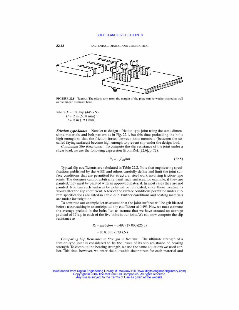
where F = 100 kip (445 kN)H = 2 in (50.8 mm)
t = 3⁄4 in (19.1 mm)
Friction-type Joints. Now let us design a friction-type joint using the same dimen-sions, materials, and bolt pattern as in Fig. 22.1, but this time preloading the boltshigh enough so that the friction forces between joint members (between the so-called faying surfaces) become high enough to prevent slip under the design load.
Computing Slip Resistance. To compute the slip resistance of the joint under ashear load, we use the following expression (from Ref. [22.6], p. 72):
RS = µSFPAbm (22.5)
Typical slip coefficients are tabulated in Table 22.2. Note that engineering speci-fications published by the AISC and others carefully define and limit the joint sur-face conditions that are permitted for structural steel work involving friction-typejoints. The designer cannot arbitrarily paint such surfaces, for example; if they arepainted, they must be painted with an approved material. In most cases they are notpainted. Nor can such surfaces be polished or lubricated, since these treatmentswould alter the slip coefficient.A few of the surface conditions permitted under cur-rent specifications are listed in Table 22.2. Further conditions and coating materialsare under investigation.
To continue our example, let us assume that the joint surfaces will be grit blastedbefore use, resulting in an anticipated slip coefficient of 0.493. Now we must estimatethe average preload in the bolts. Let us assume that we have created an averagepreload of 17 kip in each of the five bolts in our joint. We can now compute the slipresistance as
RS = µSFPAbm = 0.493 (17 000)(2)(5)
= 83 810 lb (373 kN)
Comparing Slip Resistance to Strength in Bearing. The ultimate strength of afriction-type joint is considered to be the lower of its slip resistance or bearingstrength. To compute the bearing strength, we use the same equations we used ear-lier. This time, however, we enter the allowable shear stress for each material and
22.12 FASTENING, JOINING, AND CONNECTING
FIGURE 22.5 Tearout. The pieces torn from the margin of the plate can be wedge-shaped as wellas rectilinear, as shown here.
BOLTED AND RIVETED JOINTS
Downloaded from Digital Engineering Library @ McGraw-Hill (www.digitalengineeringlibrary.com)Copyright © 2004 The McGraw-Hill Companies. All rights reserved.
Any use is subject to the Terms of Use as given at the website.
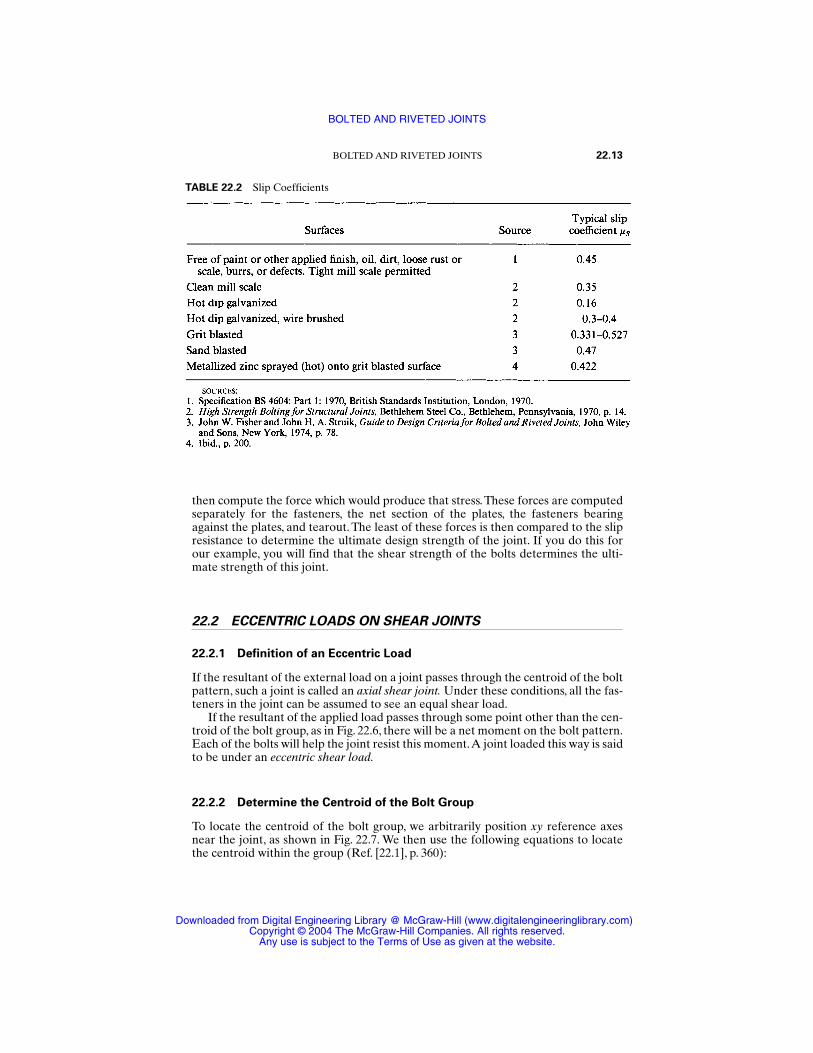
then compute the force which would produce that stress.These forces are computedseparately for the fasteners, the net section of the plates, the fasteners bearingagainst the plates, and tearout. The least of these forces is then compared to the slipresistance to determine the ultimate design strength of the joint. If you do this forour example, you will find that the shear strength of the bolts determines the ulti-mate strength of this joint.
22.2 ECCENTRIC LOADS ON SHEAR JOINTS
22.2.1 Definition of an Eccentric Load
If the resultant of the external load on a joint passes through the centroid of the boltpattern, such a joint is called an axial shear joint. Under these conditions, all the fas-teners in the joint can be assumed to see an equal shear load.
If the resultant of the applied load passes through some point other than the cen-troid of the bolt group, as in Fig. 22.6, there will be a net moment on the bolt pattern.Each of the bolts will help the joint resist this moment.A joint loaded this way is saidto be under an eccentric shear load.
22.2.2 Determine the Centroid of the Bolt Group
To locate the centroid of the bolt group, we arbitrarily position xy reference axesnear the joint, as shown in Fig. 22.7. We then use the following equations to locatethe centroid within the group (Ref. [22.1], p. 360):
BOLTED AND RIVETED JOINTS 22.13
TABLE 22.2 Slip Coefficients
BOLTED AND RIVETED JOINTS
Downloaded from Digital Engineering Library @ McGraw-Hill (www.digitalengineeringlibrary.com)Copyright © 2004 The McGraw-Hill Companies. All rights reserved.
Any use is subject to the Terms of Use as given at the website.
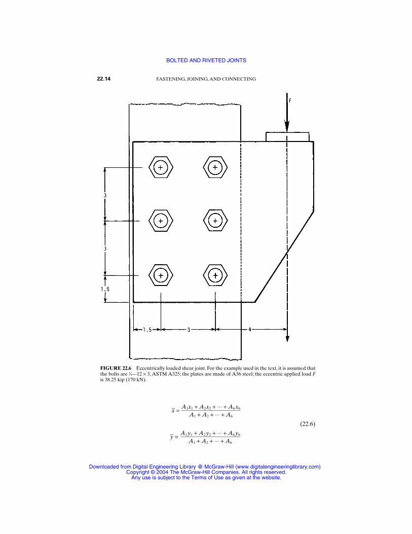
x =
y =
(22.6)
A1y1 + A2y2 + ⋅⋅⋅ + A6y6A1 + A2 + ⋅⋅⋅ + A6
A1x1 + A2x2 + ⋅⋅⋅ + A6x6A1 + A2 + ⋅⋅⋅ + A6
22.14 FASTENING, JOINING, AND CONNECTING
FIGURE 22.6 Eccentrically loaded shear joint. For the example used in the text, it is assumed thatthe bolts are 3⁄4—12 × 3, ASTM A325; the plates are made of A36 steel; the eccentric applied load Fis 38.25 kip (170 kN).
BOLTED AND RIVETED JOINTS
Downloaded from Digital Engineering Library @ McGraw-Hill (www.digitalengineeringlibrary.com)Copyright © 2004 The McGraw-Hill Companies. All rights reserved.
Any use is subject to the Terms of Use as given at the website.
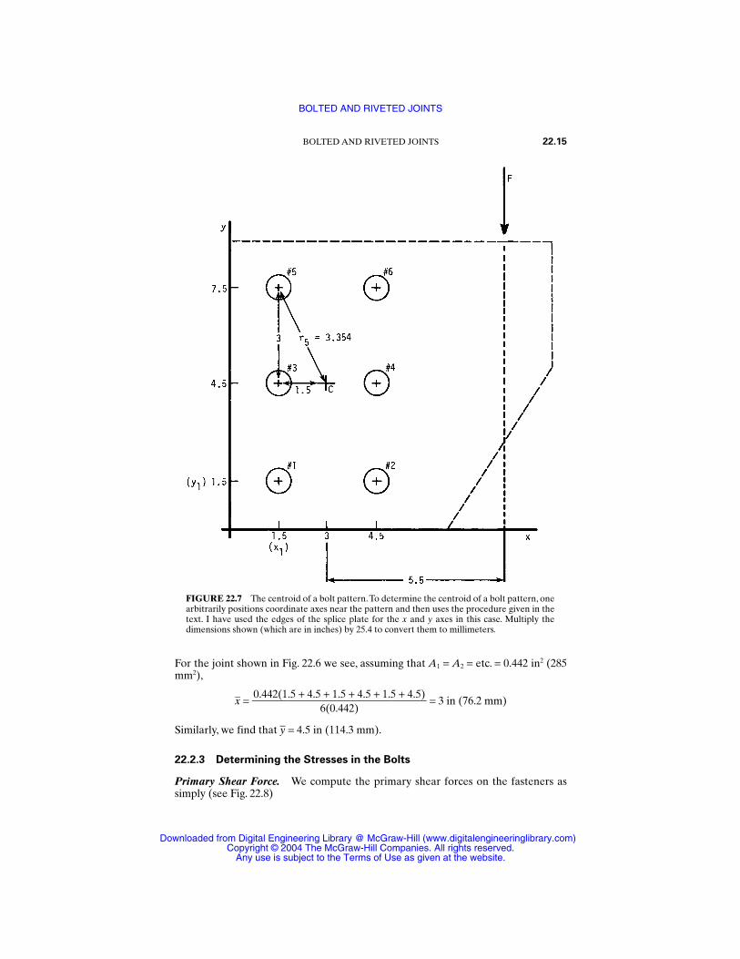
For the joint shown in Fig. 22.6 we see, assuming that A1 = A2 = etc. = 0.442 in2 (285mm2),
x = = 3 in (76.2 mm)
Similarly, we find that y = 4.5 in (114.3 mm).
22.2.3 Determining the Stresses in the Bolts
Primary Shear Force. We compute the primary shear forces on the fasteners assimply (see Fig. 22.8)
0.442(1.5 + 4.5 + 1.5 + 4.5 + 1.5 + 4.5)
6(0.442)
BOLTED AND RIVETED JOINTS 22.15
FIGURE 22.7 The centroid of a bolt pattern.To determine the centroid of a bolt pattern, onearbitrarily positions coordinate axes near the pattern and then uses the procedure given in thetext. I have used the edges of the splice plate for the x and y axes in this case. Multiply thedimensions shown (which are in inches) by 25.4 to convert them to millimeters.
BOLTED AND RIVETED JOINTS
Downloaded from Digital Engineering Library @ McGraw-Hill (www.digitalengineeringlibrary.com)Copyright © 2004 The McGraw-Hill Companies. All rights reserved.
Any use is subject to the Terms of Use as given at the website.
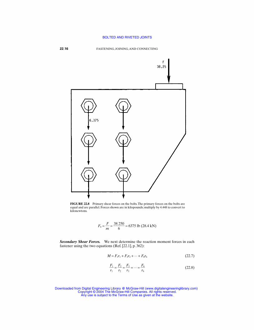
Fb = mF
= 38
6250 = 6375 lb (28.4 kN)
Secondary Shear Forces. We next determine the reaction moment forces in eachfastener using the two equations (Ref. [22.1], p. 362):
M = F1r1 + F2r2 + ⋅⋅⋅ + F6r6 (22.7)
Fr1
1 = Fr2
2 = Fr3
3 = ⋅⋅⋅ = Fr6
6 (22.8)
22.16 FASTENING, JOINING, AND CONNECTING
FIGURE 22.8 Primary shear forces on the bolts.The primary forces on the bolts areequal and are parallel. Forces shown are in kilopounds; multiply by 4.448 to convert tokilonewtons.
BOLTED AND RIVETED JOINTS
Downloaded from Digital Engineering Library @ McGraw-Hill (www.digitalengineeringlibrary.com)Copyright © 2004 The McGraw-Hill Companies. All rights reserved.
Any use is subject to the Terms of Use as given at the website.
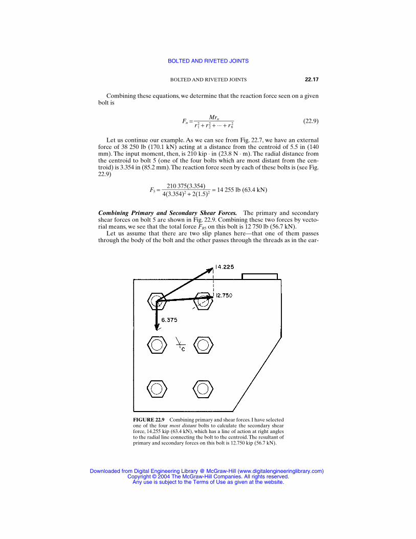
Combining these equations, we determine that the reaction force seen on a givenbolt is
Fn = (22.9)
Let us continue our example. As we can see from Fig. 22.7, we have an externalforce of 38 250 lb (170.1 kN) acting at a distance from the centroid of 5.5 in (140mm). The input moment, then, is 210 kip ⋅ in (23.8 N ⋅ m). The radial distance fromthe centroid to bolt 5 (one of the four bolts which are most distant from the cen-troid) is 3.354 in (85.2 mm).The reaction force seen by each of these bolts is (see Fig.22.9)
F5 = = 14 255 lb (63.4 kN)
Combining Primary and Secondary Shear Forces. The primary and secondaryshear forces on bolt 5 are shown in Fig. 22.9. Combining these two forces by vecto-rial means, we see that the total force FR5 on this bolt is 12 750 lb (56.7 kN).
Let us assume that there are two slip planes here—that one of them passesthrough the body of the bolt and the other passes through the threads as in the ear-
210 375(3.354)4(3.354)2 + 2(1.5)2
Mrnr 1
2 + r 22 + ⋅⋅⋅ + r 6
2
BOLTED AND RIVETED JOINTS 22.17
FIGURE 22.9 Combining primary and shear forces. I have selectedone of the four most distant bolts to calculate the secondary shearforce, 14.255 kip (63.4 kN), which has a line of action at right anglesto the radial line connecting the bolt to the centroid. The resultant ofprimary and secondary forces on this bolt is 12.750 kip (56.7 kN).
BOLTED AND RIVETED JOINTS
Downloaded from Digital Engineering Library @ McGraw-Hill (www.digitalengineeringlibrary.com)Copyright © 2004 The McGraw-Hill Companies. All rights reserved.
Any use is subject to the Terms of Use as given at the website.
lier example illustrated in Fig. 22.2. The shear area of bolt 5, therefore, is (see Sec.22.1.2 for the equations) 0.793 in2 (511 mm2).
We can now compute the shear stress within this bolt:
τ = FA
R
5
5 = 102.779530
= 16 078 psi
This is less than the maximum shear stress allowed for A325 steel bolts (see Table22.1), and so the design is acceptable.
It is informative to compare these results with those obtained in Sec. 22.1.3,where we analyzed a joint having similar dimensions, the same input load, and oneless bolt.The axial load in the earlier case created a shear stress of only 9646 psi (66.5MPa) in each bolt. When the same load is applied eccentrically, passing 5.5 in fromthe centroid, it creates 16 078/9646 times as much stress in the most distant bolts,even though there are more bolts this time to take the load. Be warned!
22.3 TENSION-LOADED JOINTS: PRELOADINGOF BOLTS
In the joints discussed so far, the bolts or rivets were loaded in shear. Such joints areusually encountered in structural steel work. Most other bolted joints in this worldare loaded primarily in tension—with the applied loads more or less parallel to theaxis of the bolts.
The analysis of tension joints usually centers on an analysis of the tension in thefasteners: first with the initial or preload in the fasteners when they are initially tight-ened, and then with the working loads that exist in the fasteners and in the jointmembers when external forces are applied to the joint as the product or structure isput into use. These working loads consist of the preload plus or minus some portionof the external load seen by the joint in use.
Because clamping force is essential when a joint has to resist tension loads, rivetsare rarely used. The following discussion, therefore, will focus on bolted joints. Theanalytical procedure described, however, could be used with riveted joints if thedesigner is able to estimate the initial preload in the rivets.
22.3.1 Preliminary Design and Calculations
Estimate External Loads. The first step in the design procedure is to estimate theexternal loads which will be seen by each bolted joint. Such loads can be static,dynamic, or impact in nature.They can be created by weights such as snow, water, orother parts of the structure.They can be created by inertial forces, by shock or vibra-tion, by changes in temperature, by fluid pressure, or by prime movers.
Fastener Stiffness. The next step is to compute the stiffness or spring rate of thefasteners using the following equation:
kB = (22.10)ASABE
LSAB + LBAS
22.18 FASTENING, JOINING, AND CONNECTING
BOLTED AND RIVETED JOINTS
Downloaded from Digital Engineering Library @ McGraw-Hill (www.digitalengineeringlibrary.com)Copyright © 2004 The McGraw-Hill Companies. All rights reserved.
Any use is subject to the Terms of Use as given at the website.
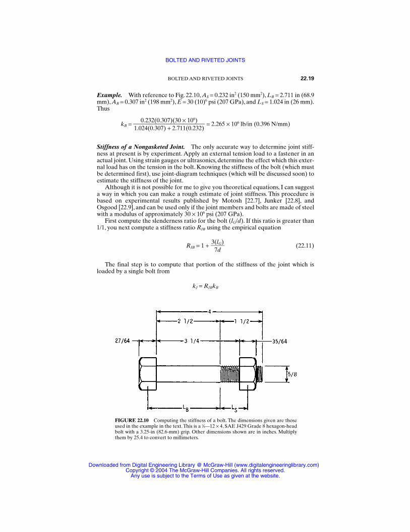
Example. With reference to Fig. 22.10, AS = 0.232 in2 (150 mm2), LB = 2.711 in (68.9mm), AB = 0.307 in2 (198 mm2), E = 30 (10)6 psi (207 GPa), and LS = 1.024 in (26 mm).Thus
kB = = 2.265 × 10⁶ lb/in (0.396 N/mm)
Stiffness of a Nongasketed Joint. The only accurate way to determine joint stiff-ness at present is by experiment. Apply an external tension load to a fastener in anactual joint. Using strain gauges or ultrasonics, determine the effect which this exter-nal load has on the tension in the bolt. Knowing the stiffness of the bolt (which mustbe determined first), use joint-diagram techniques (which will be discussed soon) toestimate the stiffness of the joint.
Although it is not possible for me to give you theoretical equations, I can suggesta way in which you can make a rough estimate of joint stiffness. This procedure isbased on experimental results published by Motosh [22.7], Junker [22.8], andOsgood [22.9], and can be used only if the joint members and bolts are made of steelwith a modulus of approximately 30 × 106 psi (207 GPa).
First compute the slenderness ratio for the bolt (lG/d). If this ratio is greater than1/1, you next compute a stiffness ratio RJB using the empirical equation
RJB = 1 + (22.11)
The final step is to compute that portion of the stiffness of the joint which isloaded by a single bolt from
kJ = RJBkB
3(lG)
7d
0.232(0.307)(30 × 106)1.024(0.307) + 2.711(0.232)
BOLTED AND RIVETED JOINTS 22.19
FIGURE 22.10 Computing the stiffness of a bolt. The dimensions given are thoseused in the example in the text.This is a 5⁄8—12 × 4, SAE J429 Grade 8 hexagon-headbolt with a 3.25-in (82.6-mm) grip. Other dimensions shown are in inches. Multiplythem by 25.4 to convert to millimeters.
BOLTED AND RIVETED JOINTS
Downloaded from Digital Engineering Library @ McGraw-Hill (www.digitalengineeringlibrary.com)Copyright © 2004 The McGraw-Hill Companies. All rights reserved.
Any use is subject to the Terms of Use as given at the website.
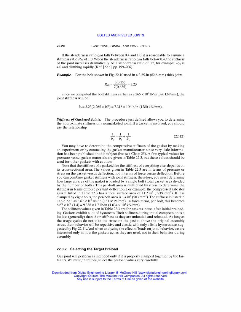
If the slenderness ratio lG/d falls between 0.4 and 1.0, it is reasonable to assume astiffness ratio RJB of 1.0. When the slenderness ratio lG/d falls below 0.4, the stiffnessof the joint increases dramatically. At a slenderness ratio of 0.2, for example, RJB is4.0 and climbing rapidly (Ref. [22.6], pp. 199–206).
Example. For the bolt shown in Fig. 22.10 used in a 3.25-in (82.6-mm) thick joint,
RJB = = 3.23
Since we computed the bolt stiffness earlier as 2.265 × 10⁶ lb/in (396 kN/mm), thejoint stiffness will be
kJ = 3.23(2.265 × 10⁶) = 7.316 × 10⁶ lb/in (1280 kN/mm).
Stiffness of Gasketed Joints. The procedure just defined allows you to determinethe approximate stiffness of a nongasketed joint. If a gasket is involved, you shoulduse the relationship
k1
T =
k1
J +
k1G (22.12)
You may have to determine the compressive stiffness of the gasket by makingan experiment or by contacting the gasket manufacturer, since very little informa-tion has been published on this subject (but see Chap. 25). A few typical values forpressure-vessel gasket materials are given in Table 22.3, but these values should beused for other gaskets with caution.
Note that the stiffness of a gasket, like the stiffness of everything else, depends onits cross-sectional area. The values given in Table 22.3 are in terms of pressure orstress on the gasket versus deflection, not in terms of force versus deflection. Beforeyou can combine gasket stiffness with joint stiffness, therefore, you must determinehow large an area of the gasket is loaded by a single bolt (total gasket area dividedby the number of bolts). This per-bolt area is multiplied by stress to determine thestiffness in terms of force per unit deflection. For example, the compressed asbestosgasket listed in Table 22.3 has a total surface area of 11.2 in2 (7219 mm2). If it isclamped by eight bolts, the per-bolt area is 1.4 in2 (903 mm2).The stiffness is listed inTable 22.3 as 6.67 × 10² ksi/in (181 MPa/mm). In force terms, per bolt, this becomes6.67 × 105 (1.4) = 9.338 × 10⁵ lb/in (1.634 × 10² kN/mm).
The stiffness values given in Table 22.3 are for gaskets in use, after initial preload-ing. Gaskets exhibit a lot of hysteresis. Their stiffness during initial compression is alot less (generally) than their stiffness as they are unloaded and reloaded.As long asthe usage cycles do not take the stress on the gasket above the original assemblystress, their behavior will be repetitive and elastic, with only a little hysteresis, as sug-gested by Fig. 22.11.And when analyzing the effect of loads on joint behavior, we areinterested only in how the gaskets act as they are used, not in their behavior duringassembly.
22.3.2 Selecting the Target Preload
Our joint will perform as intended only if it is properly clamped together by the fas-teners. We must, therefore, select the preload values very carefully.
3(3.25)7(0.625)
22.20 FASTENING, JOINING, AND CONNECTING
BOLTED AND RIVETED JOINTS
Downloaded from Digital Engineering Library @ McGraw-Hill (www.digitalengineeringlibrary.com)Copyright © 2004 The McGraw-Hill Companies. All rights reserved.
Any use is subject to the Terms of Use as given at the website.
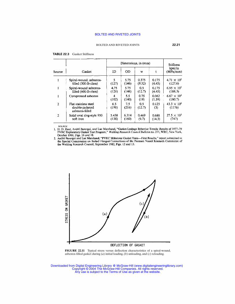
BOLTED AND RIVETED JOINTS 22.21
TABLE 22.3 Gasket Stiffness
FIGURE 22.11 Typical stress versus deflection characteristics of a spiral-wound,asbestos-filled gasket during (a) initial loading, (b) unloading, and (c) reloading.
BOLTED AND RIVETED JOINTS
Downloaded from Digital Engineering Library @ McGraw-Hill (www.digitalengineeringlibrary.com)Copyright © 2004 The McGraw-Hill Companies. All rights reserved.
Any use is subject to the Terms of Use as given at the website.
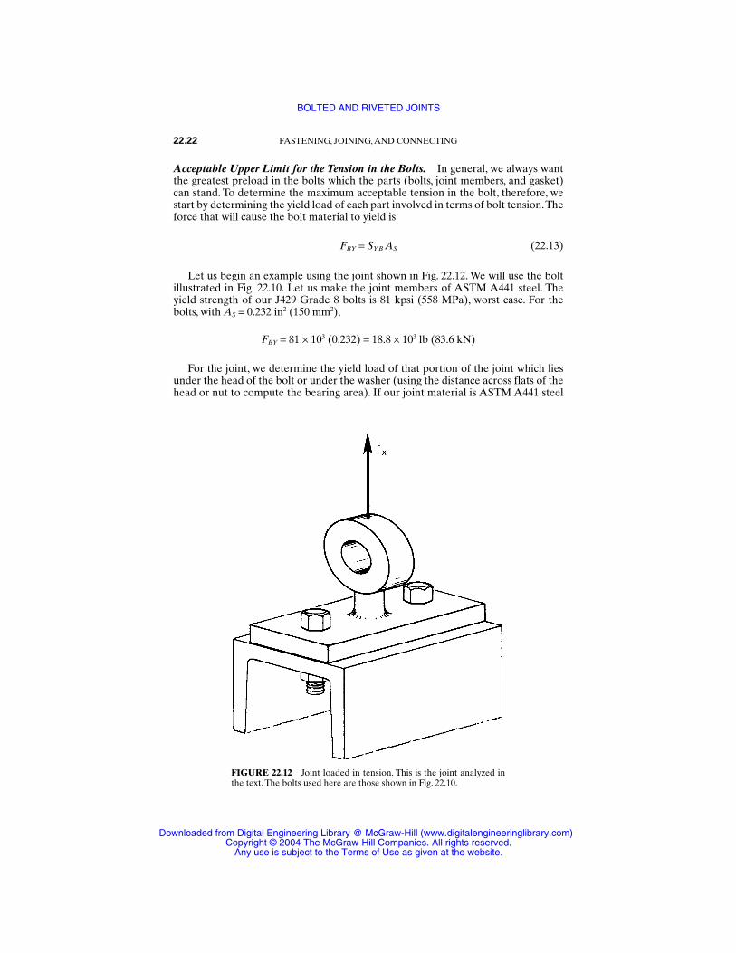
Acceptable Upper Limit for the Tension in the Bolts. In general, we always wantthe greatest preload in the bolts which the parts (bolts, joint members, and gasket)can stand. To determine the maximum acceptable tension in the bolt, therefore, westart by determining the yield load of each part involved in terms of bolt tension.Theforce that will cause the bolt material to yield is
FBY = SYB AS (22.13)
Let us begin an example using the joint shown in Fig. 22.12. We will use the boltillustrated in Fig. 22.10. Let us make the joint members of ASTM A441 steel. Theyield strength of our J429 Grade 8 bolts is 81 kpsi (558 MPa), worst case. For thebolts, with AS = 0.232 in2 (150 mm2),
FBY = 81 × 103 (0.232) = 18.8 × 10³ lb (83.6 kN)
For the joint, we determine the yield load of that portion of the joint which liesunder the head of the bolt or under the washer (using the distance across flats of thehead or nut to compute the bearing area). If our joint material is ASTM A441 steel
22.22 FASTENING, JOINING, AND CONNECTING
FIGURE 22.12 Joint loaded in tension. This is the joint analyzed inthe text. The bolts used here are those shown in Fig. 22.10.
BOLTED AND RIVETED JOINTS
Downloaded from Digital Engineering Library @ McGraw-Hill (www.digitalengineeringlibrary.com)Copyright © 2004 The McGraw-Hill Companies. All rights reserved.
Any use is subject to the Terms of Use as given at the website.

with a yield strength of 40 kpsi (276 MPa), we would find that a bolt force of 27.6 kip(122 kN) would yield the joint. We take the lesser of the joint or bolt yield loads,18.8 × 103 lb (83.6 kN) as the yield load of the system.
Next, since we are planning to tighten these fasteners by applying torque to thenuts, we subtract 10 percent from the yield strength of the fastener to allow for thetorsional stresses which will be developed in the fastener as it is tightened. If wewere planning to use a high-pressure lubricant on the threads, we might subtractonly 2 to 4 percent for torsion. Since no lube will be used in our example, we subtract10 percent, making the upper limit 16.9 × 10³ lb (75.2 kN).
This will remain our upper limit unless the fasteners will also be subjected toshear stress; or unless code limits, stress corrosion problems, or the desire for asafety factor forces us to reduce it further.We will assume, in our example, that theydo not.
Before continuing, however, let us see what we would have to do if the bolts didsee a combined tension and shear load.This might happen, for example, in a bearing-type joint in which we planned to preload (tension) the bolts to a significant per-centage of yield.There are other types of joint, of course, which are subjected to bothtensile and shear loads in use. Any shear load on the bolt will “use up” part of thestrength of the bolt, leaving less capacity for tensile loads (Ref. [22.6], p. 226).
Under these conditions, the maximum acceptable tensile stress in a bolt can bedetermined using any of the static failure theories of Chap. 28. Here, we select theequation
Sλ
2
+ φ2 = 1 (22.14)
where S = the ratio of the shear strength to the tensile strength (typically 0.6) for boltsteels. Equation (22.14) is a form of the maximum-shear-stress theory.
Acceptable Lower Limit for the Clamping Force on the Joint. When we are com-puting the maximum acceptable forces, we focus on the joint, because its behaviorcan be seriously affected if the interface forces become too small. The joint, forexample, might leak, it might vibrate loose, or it might have a short fatigue life. Todetermine the lower acceptable limit, we must consider each potential failure modeseparately, estimate the minimum preload required to control that particular prob-lem, and then select the highest of these several minimum requirements to establishthe minimum for the system.
This is one of the more difficult steps of our procedure. In fact, we may be able todetermine the acceptable minimum preload only by making fatigue or vibrationtests or the like. (We will consider fatigue problems at length in Sec. 22.5.) There aresome rules of thumb, however, which we can apply.
If our joint is a friction-type shear joint, or if it will be subjected to transversevibration, we want a minimum preload which will prevent joint slip under the maxi-mum anticipated shear load. This load is
FC (min) ≥ FS
X (22.15)
If we are dealing with a foundation bolt or something where it is only necessary toavoid separation of the joint members, the minimum acceptable preload can be zero.If we are dealing with a gasketed joint, we will have to worry about the minimumacceptable gasket pressure required to keep that gasket from leaking.
BOLTED AND RIVETED JOINTS 22.23
BOLTED AND RIVETED JOINTS
Downloaded from Digital Engineering Library @ McGraw-Hill (www.digitalengineeringlibrary.com)Copyright © 2004 The McGraw-Hill Companies. All rights reserved.
Any use is subject to the Terms of Use as given at the website.
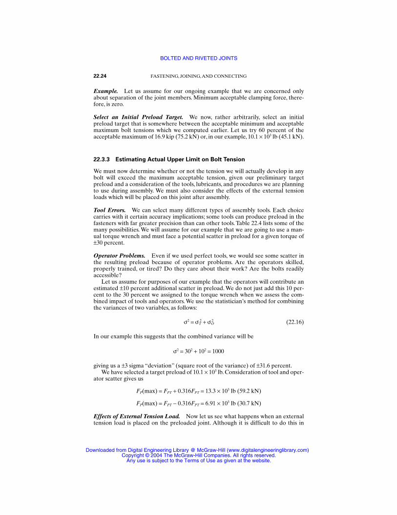
Example. Let us assume for our ongoing example that we are concerned onlyabout separation of the joint members. Minimum acceptable clamping force, there-fore, is zero.
Select an Initial Preload Target. We now, rather arbitrarily, select an initialpreload target that is somewhere between the acceptable minimum and acceptablemaximum bolt tensions which we computed earlier. Let us try 60 percent of theacceptable maximum of 16.9 kip (75.2 kN) or, in our example, 10.1 × 10³ lb (45.1 kN).
22.3.3 Estimating Actual Upper Limit on Bolt Tension
We must now determine whether or not the tension we will actually develop in anybolt will exceed the maximum acceptable tension, given our preliminary targetpreload and a consideration of the tools, lubricants, and procedures we are planningto use during assembly. We must also consider the effects of the external tensionloads which will be placed on this joint after assembly.
Tool Errors. We can select many different types of assembly tools. Each choicecarries with it certain accuracy implications; some tools can produce preload in thefasteners with far greater precision than can other tools. Table 22.4 lists some of themany possibilities. We will assume for our example that we are going to use a man-ual torque wrench and must face a potential scatter in preload for a given torque of±30 percent.
Operator Problems. Even if we used perfect tools, we would see some scatter inthe resulting preload because of operator problems. Are the operators skilled,properly trained, or tired? Do they care about their work? Are the bolts readilyaccessible?
Let us assume for purposes of our example that the operators will contribute anestimated ±10 percent additional scatter in preload. We do not just add this 10 per-cent to the 30 percent we assigned to the torque wrench when we assess the com-bined impact of tools and operators. We use the statistician’s method for combiningthe variances of two variables, as follows:
ç2 = çT2 + çO
2 (22.16)
In our example this suggests that the combined variance will be
ç2 = 302 + 102 = 1000
giving us a ±3 sigma “deviation” (square root of the variance) of ±31.6 percent.We have selected a target preload of 10.1 × 10³ lb. Consideration of tool and oper-
ator scatter gives us
FP(max) = FPT + 0.316FPT = 13.3 × 10³ lb (59.2 kN)
FP(max) = FPT − 0.316FPT = 6.91 × 10³ lb (30.7 kN)
Effects of External Tension Load. Now let us see what happens when an externaltension load is placed on the preloaded joint. Although it is difficult to do this in
22.24 FASTENING, JOINING, AND CONNECTING
BOLTED AND RIVETED JOINTS
Downloaded from Digital Engineering Library @ McGraw-Hill (www.digitalengineeringlibrary.com)Copyright © 2004 The McGraw-Hill Companies. All rights reserved.
Any use is subject to the Terms of Use as given at the website.
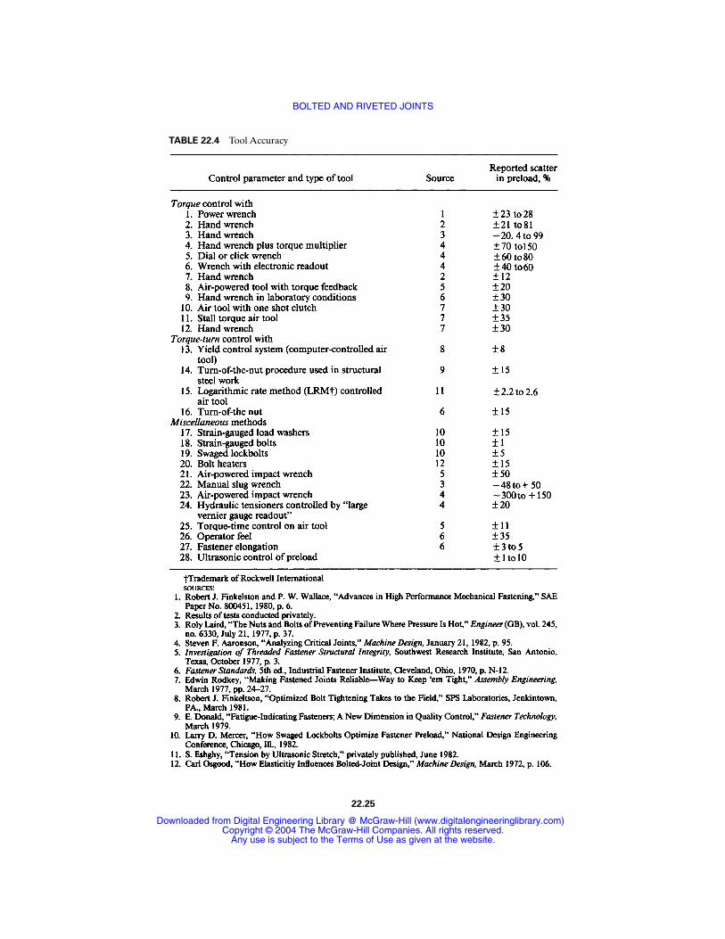
TABLE 22.4 Tool Accuracy
22.25
BOLTED AND RIVETED JOINTS
Downloaded from Digital Engineering Library @ McGraw-Hill (www.digitalengineeringlibrary.com)Copyright © 2004 The McGraw-Hill Companies. All rights reserved.
Any use is subject to the Terms of Use as given at the website.
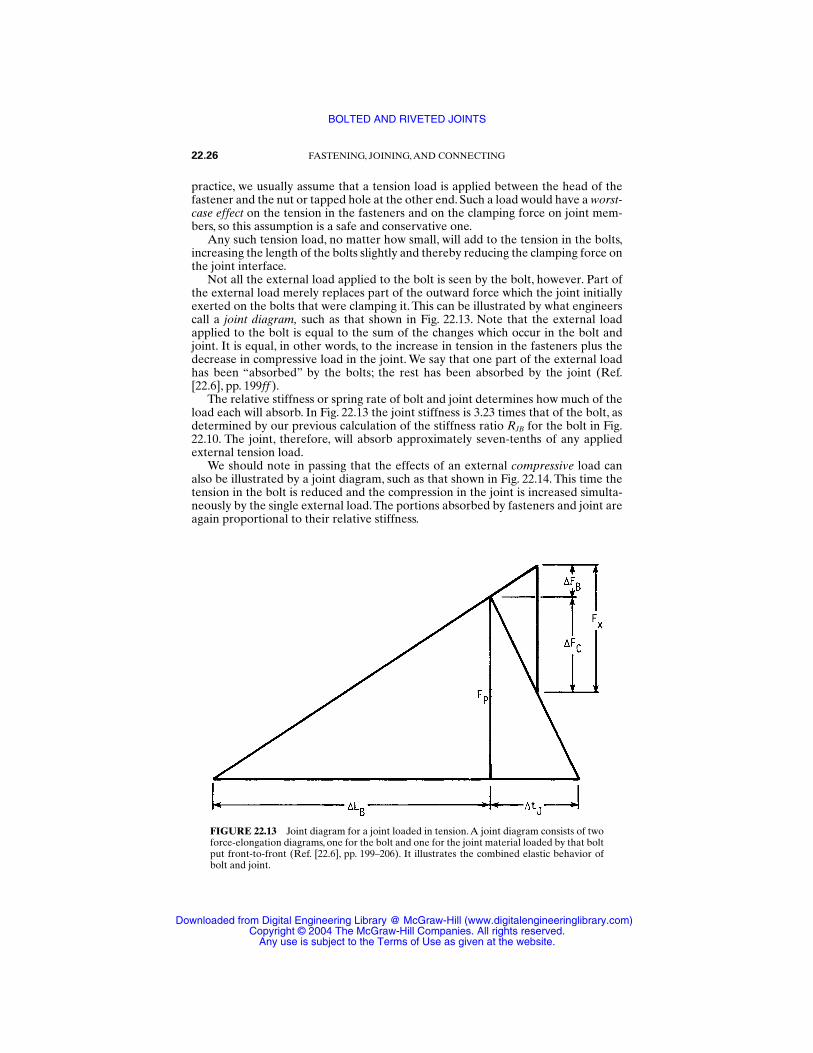
practice, we usually assume that a tension load is applied between the head of thefastener and the nut or tapped hole at the other end. Such a load would have a worst-case effect on the tension in the fasteners and on the clamping force on joint mem-bers, so this assumption is a safe and conservative one.
Any such tension load, no matter how small, will add to the tension in the bolts,increasing the length of the bolts slightly and thereby reducing the clamping force onthe joint interface.
Not all the external load applied to the bolt is seen by the bolt, however. Part ofthe external load merely replaces part of the outward force which the joint initiallyexerted on the bolts that were clamping it. This can be illustrated by what engineerscall a joint diagram, such as that shown in Fig. 22.13. Note that the external loadapplied to the bolt is equal to the sum of the changes which occur in the bolt andjoint. It is equal, in other words, to the increase in tension in the fasteners plus thedecrease in compressive load in the joint. We say that one part of the external loadhas been “absorbed” by the bolts; the rest has been absorbed by the joint (Ref.[22.6], pp. 199ff ).
The relative stiffness or spring rate of bolt and joint determines how much of theload each will absorb. In Fig. 22.13 the joint stiffness is 3.23 times that of the bolt, asdetermined by our previous calculation of the stiffness ratio RJB for the bolt in Fig.22.10. The joint, therefore, will absorb approximately seven-tenths of any appliedexternal tension load.
We should note in passing that the effects of an external compressive load canalso be illustrated by a joint diagram, such as that shown in Fig. 22.14. This time thetension in the bolt is reduced and the compression in the joint is increased simulta-neously by the single external load.The portions absorbed by fasteners and joint areagain proportional to their relative stiffness.
22.26 FASTENING, JOINING, AND CONNECTING
FIGURE 22.13 Joint diagram for a joint loaded in tension.A joint diagram consists of twoforce-elongation diagrams, one for the bolt and one for the joint material loaded by that boltput front-to-front (Ref. [22.6], pp. 199–206). It illustrates the combined elastic behavior ofbolt and joint.
BOLTED AND RIVETED JOINTS
Downloaded from Digital Engineering Library @ McGraw-Hill (www.digitalengineeringlibrary.com)Copyright © 2004 The McGraw-Hill Companies. All rights reserved.
Any use is subject to the Terms of Use as given at the website.
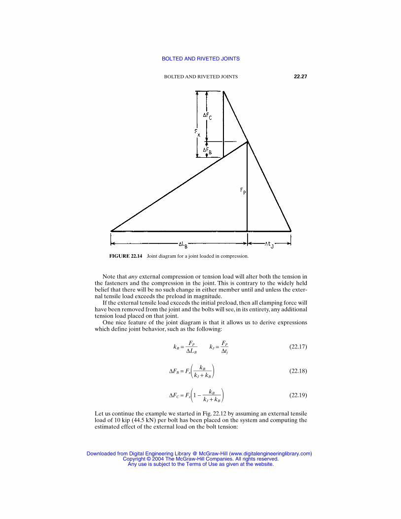
Note that any external compression or tension load will alter both the tension inthe fasteners and the compression in the joint. This is contrary to the widely heldbelief that there will be no such change in either member until and unless the exter-nal tensile load exceeds the preload in magnitude.
If the external tensile load exceeds the initial preload, then all clamping force willhave been removed from the joint and the bolts will see, in its entirety, any additionaltension load placed on that joint.
One nice feature of the joint diagram is that it allows us to derive expressionswhich define joint behavior, such as the following:
kB = kJ = (22.17)
∆FB = FxkJ
k+
B
kB (22.18)
∆FC = Fx1 − (22.19)
Let us continue the example we started in Fig. 22.12 by assuming an external tensileload of 10 kip (44.5 kN) per bolt has been placed on the system and computing theestimated effect of the external load on the bolt tension:
kBkJ + kB
FP∆tj
FP∆LB
BOLTED AND RIVETED JOINTS 22.27
FIGURE 22.14 Joint diagram for a joint loaded in compression.
BOLTED AND RIVETED JOINTS
Downloaded from Digital Engineering Library @ McGraw-Hill (www.digitalengineeringlibrary.com)Copyright © 2004 The McGraw-Hill Companies. All rights reserved.
Any use is subject to the Terms of Use as given at the website.
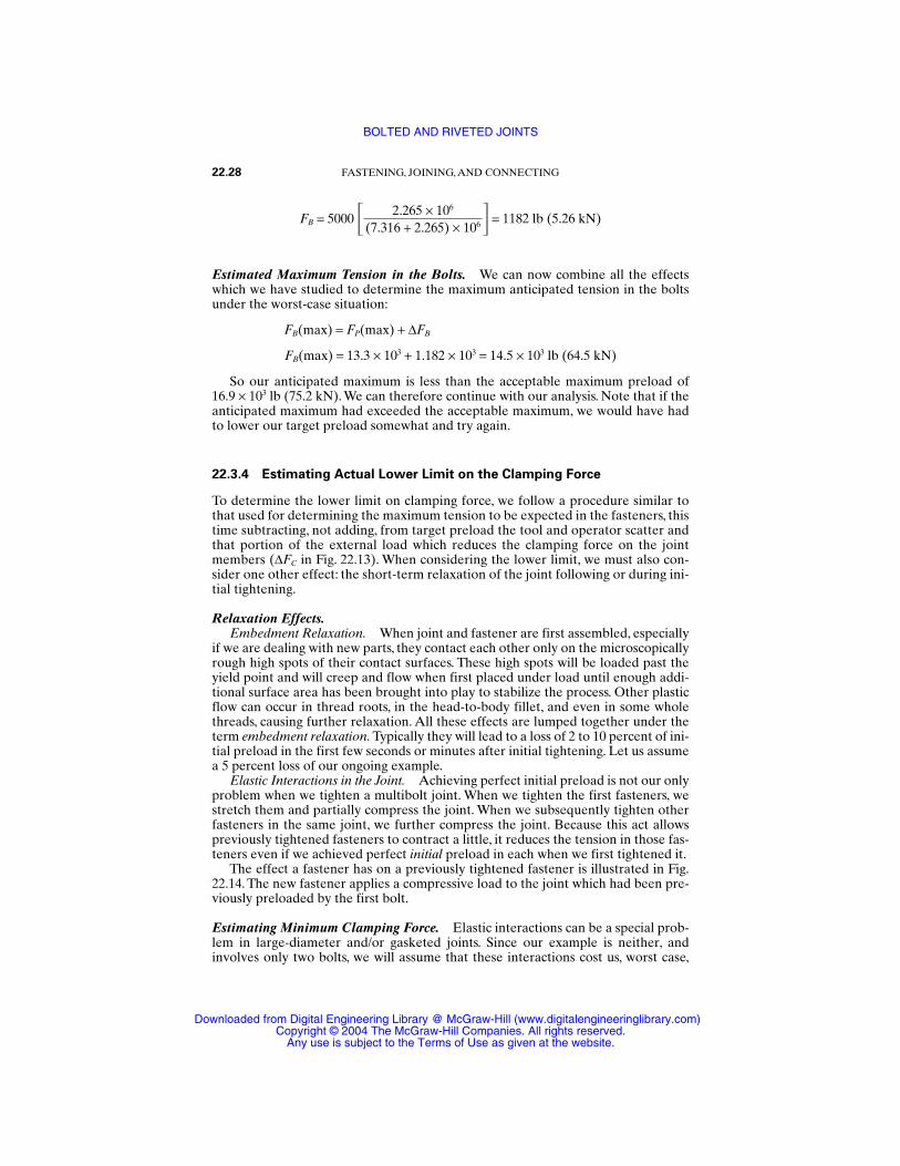
FB = 5000 = 1182 lb (5.26 kN)
Estimated Maximum Tension in the Bolts. We can now combine all the effectswhich we have studied to determine the maximum anticipated tension in the boltsunder the worst-case situation:
FB(max) = FP(max) + ∆FB
FB(max) = 13.3 × 10³ + 1.182 × 103 = 14.5 × 10³ lb (64.5 kN)
So our anticipated maximum is less than the acceptable maximum preload of 16.9 × 10³ lb (75.2 kN). We can therefore continue with our analysis. Note that if theanticipated maximum had exceeded the acceptable maximum, we would have hadto lower our target preload somewhat and try again.
22.3.4 Estimating Actual Lower Limit on the Clamping Force
To determine the lower limit on clamping force, we follow a procedure similar tothat used for determining the maximum tension to be expected in the fasteners, thistime subtracting, not adding, from target preload the tool and operator scatter andthat portion of the external load which reduces the clamping force on the jointmembers (∆FC in Fig. 22.13). When considering the lower limit, we must also con-sider one other effect: the short-term relaxation of the joint following or during ini-tial tightening.
Relaxation Effects.Embedment Relaxation. When joint and fastener are first assembled, especially
if we are dealing with new parts, they contact each other only on the microscopicallyrough high spots of their contact surfaces. These high spots will be loaded past theyield point and will creep and flow when first placed under load until enough addi-tional surface area has been brought into play to stabilize the process. Other plasticflow can occur in thread roots, in the head-to-body fillet, and even in some wholethreads, causing further relaxation. All these effects are lumped together under theterm embedment relaxation. Typically they will lead to a loss of 2 to 10 percent of ini-tial preload in the first few seconds or minutes after initial tightening. Let us assumea 5 percent loss of our ongoing example.
Elastic Interactions in the Joint. Achieving perfect initial preload is not our onlyproblem when we tighten a multibolt joint. When we tighten the first fasteners, westretch them and partially compress the joint. When we subsequently tighten otherfasteners in the same joint, we further compress the joint. Because this act allowspreviously tightened fasteners to contract a little, it reduces the tension in those fas-teners even if we achieved perfect initial preload in each when we first tightened it.
The effect a fastener has on a previously tightened fastener is illustrated in Fig.22.14. The new fastener applies a compressive load to the joint which had been pre-viously preloaded by the first bolt.
Estimating Minimum Clamping Force. Elastic interactions can be a special prob-lem in large-diameter and/or gasketed joints. Since our example is neither, andinvolves only two bolts, we will assume that these interactions cost us, worst case,
2.265 × 10⁶
(7.316 + 2.265) × 106
22.28 FASTENING, JOINING, AND CONNECTING
BOLTED AND RIVETED JOINTS
Downloaded from Digital Engineering Library @ McGraw-Hill (www.digitalengineeringlibrary.com)Copyright © 2004 The McGraw-Hill Companies. All rights reserved.
Any use is subject to the Terms of Use as given at the website.
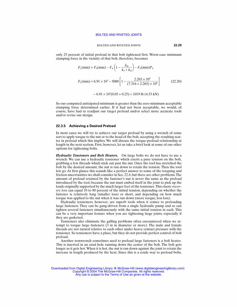
only 25 percent of initial preload in that bolt tightened first. Worst-case minimumclamping force in the vicinity of that bolt, therefore, becomes
FC(min) = FP(min) − FX 1 − − FP(min)PZ
FC(min) = 6.91 × 10³ − 5000 1 − (22.20)
− 6.91 × 10³(0.05 + 0.25) = 1019 lb (4.53 kN)
So our computed anticipated minimum is greater than the zero minimum acceptableclamping force determined earlier. If it had not been acceptable, we would, ofcourse, have had to readjust our target preload and/or select more accurate toolsand/or revise our design.
22.3.5 Achieving a Desired Preload
In most cases we will try to achieve our target preload by using a wrench of somesort to apply torque to the nut or to the head of the bolt, accepting the resulting scat-ter in preload which this implies. We will discuss the torque-preload relationship atlength in the next section. First, however, let us take a brief look at some of our otheroptions for tightening bolts.
Hydraulic Tensioners and Bolt Heaters. On large bolts we do not have to use awrench. We can use a hydraulic tensioner which exerts a pure tension on the bolt,grabbing a few threads which stick out past the nut. Once the tool has stretched thebolt by the desired amount, the nut is run down to retain the tension. Then the toollets go. At first glance this sounds like a perfect answer to some of the torquing andfriction uncertainties we shall consider in Sec. 22.4, but there are other problems.Theamount of preload retained by the fastener’s nut is never the same as the preloadintroduced by the tool, because the nut must embed itself in the joint to pick up theloads originally supported by the much larger feet of the tensioner.This elastic recov-ery loss can equal 10 to 80 percent of the initial tension, depending on whether thefastener is relatively long (smaller loss) or short, and depending on how muchtorque was applied to the nut when it was run down (more torque, less loss).
Hydraulic tensioners, however, are superb tools when it comes to preloadinglarge fasteners. They can be gang-driven from a single hydraulic pump and so cantighten several fasteners simultaneously with the same initial tension in each. Thiscan be a very important feature when you are tightening large joints, especially ifthey are gasketed.
Tensioners also eliminate the galling problems often encountered when we at-tempt to torque large fasteners (3 in in diameter or more). The male and femalethreads are not turned relative to each other under heavy contact pressure with thetensioner. So tensioners have a place, but they do not provide perfect control of boltpreload.
Another nonwrench sometimes used to preload large fasteners is a bolt heater.This is inserted in an axial hole running down the center of the bolt. The bolt getslonger as it gets hot.When it is hot, the nut is run down against the joint to retain theincrease in length produced by the heat. Since this is a crude way to preload bolts,
2.265 × 10⁶
(7.316 + 2.265) × 106
kBkJ + kB
BOLTED AND RIVETED JOINTS 22.29
BOLTED AND RIVETED JOINTS
Downloaded from Digital Engineering Library @ McGraw-Hill (www.digitalengineeringlibrary.com)Copyright © 2004 The McGraw-Hill Companies. All rights reserved.
Any use is subject to the Terms of Use as given at the website.
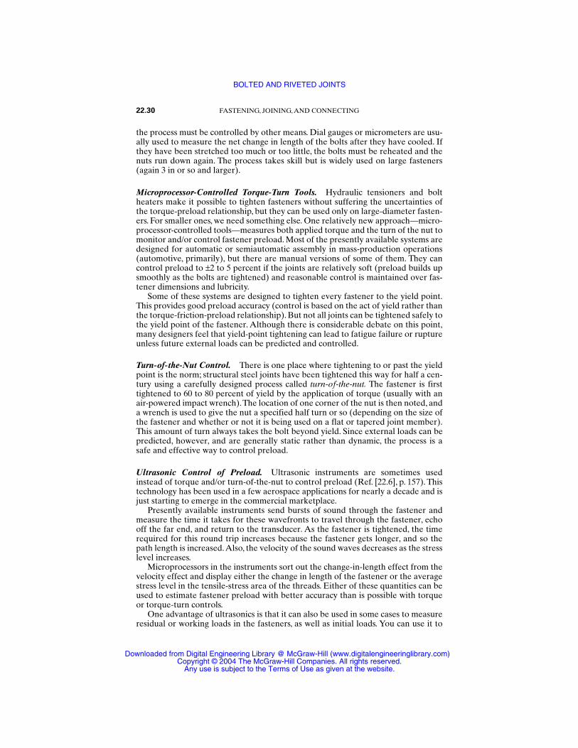
the process must be controlled by other means. Dial gauges or micrometers are usu-ally used to measure the net change in length of the bolts after they have cooled. Ifthey have been stretched too much or too little, the bolts must be reheated and thenuts run down again. The process takes skill but is widely used on large fasteners(again 3 in or so and larger).
Microprocessor-Controlled Torque-Turn Tools. Hydraulic tensioners and boltheaters make it possible to tighten fasteners without suffering the uncertainties ofthe torque-preload relationship, but they can be used only on large-diameter fasten-ers. For smaller ones, we need something else. One relatively new approach—micro-processor-controlled tools—measures both applied torque and the turn of the nut tomonitor and/or control fastener preload. Most of the presently available systems aredesigned for automatic or semiautomatic assembly in mass-production operations(automotive, primarily), but there are manual versions of some of them. They cancontrol preload to ±2 to 5 percent if the joints are relatively soft (preload builds upsmoothly as the bolts are tightened) and reasonable control is maintained over fas-tener dimensions and lubricity.
Some of these systems are designed to tighten every fastener to the yield point.This provides good preload accuracy (control is based on the act of yield rather thanthe torque-friction-preload relationship). But not all joints can be tightened safely tothe yield point of the fastener. Although there is considerable debate on this point,many designers feel that yield-point tightening can lead to fatigue failure or ruptureunless future external loads can be predicted and controlled.
Turn-of-the-Nut Control. There is one place where tightening to or past the yieldpoint is the norm; structural steel joints have been tightened this way for half a cen-tury using a carefully designed process called turn-of-the-nut. The fastener is firsttightened to 60 to 80 percent of yield by the application of torque (usually with anair-powered impact wrench).The location of one corner of the nut is then noted, anda wrench is used to give the nut a specified half turn or so (depending on the size ofthe fastener and whether or not it is being used on a flat or tapered joint member).This amount of turn always takes the bolt beyond yield. Since external loads can bepredicted, however, and are generally static rather than dynamic, the process is asafe and effective way to control preload.
Ultrasonic Control of Preload. Ultrasonic instruments are sometimes usedinstead of torque and/or turn-of-the-nut to control preload (Ref. [22.6], p. 157). Thistechnology has been used in a few aerospace applications for nearly a decade and isjust starting to emerge in the commercial marketplace.
Presently available instruments send bursts of sound through the fastener andmeasure the time it takes for these wavefronts to travel through the fastener, echooff the far end, and return to the transducer. As the fastener is tightened, the timerequired for this round trip increases because the fastener gets longer, and so thepath length is increased.Also, the velocity of the sound waves decreases as the stresslevel increases.
Microprocessors in the instruments sort out the change-in-length effect from thevelocity effect and display either the change in length of the fastener or the averagestress level in the tensile-stress area of the threads. Either of these quantities can beused to estimate fastener preload with better accuracy than is possible with torqueor torque-turn controls.
One advantage of ultrasonics is that it can also be used in some cases to measureresidual or working loads in the fasteners, as well as initial loads. You can use it to
22.30 FASTENING, JOINING, AND CONNECTING
BOLTED AND RIVETED JOINTS
Downloaded from Digital Engineering Library @ McGraw-Hill (www.digitalengineeringlibrary.com)Copyright © 2004 The McGraw-Hill Companies. All rights reserved.
Any use is subject to the Terms of Use as given at the website.
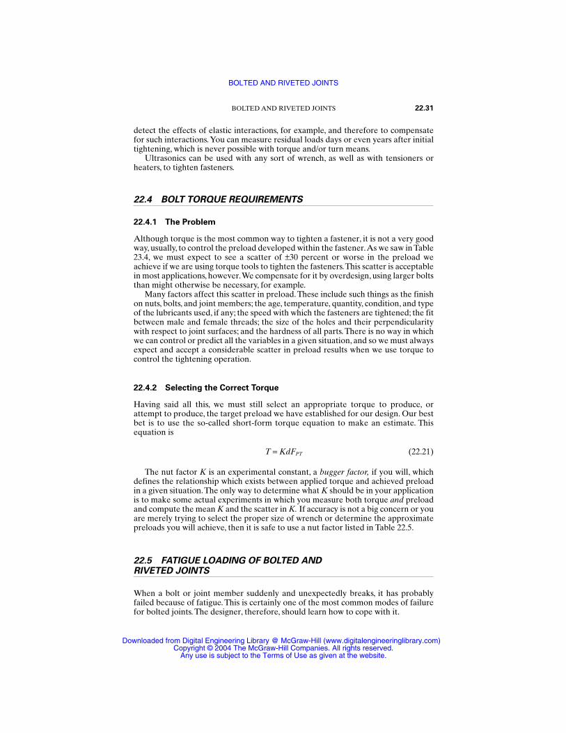
detect the effects of elastic interactions, for example, and therefore to compensatefor such interactions. You can measure residual loads days or even years after initialtightening, which is never possible with torque and/or turn means.
Ultrasonics can be used with any sort of wrench, as well as with tensioners orheaters, to tighten fasteners.
22.4 BOLT TORQUE REQUIREMENTS
22.4.1 The Problem
Although torque is the most common way to tighten a fastener, it is not a very goodway, usually, to control the preload developed within the fastener.As we saw in Table23.4, we must expect to see a scatter of ±30 percent or worse in the preload weachieve if we are using torque tools to tighten the fasteners.This scatter is acceptablein most applications, however.We compensate for it by overdesign, using larger boltsthan might otherwise be necessary, for example.
Many factors affect this scatter in preload. These include such things as the finishon nuts, bolts, and joint members; the age, temperature, quantity, condition, and typeof the lubricants used, if any; the speed with which the fasteners are tightened; the fitbetween male and female threads; the size of the holes and their perpendicularitywith respect to joint surfaces; and the hardness of all parts. There is no way in whichwe can control or predict all the variables in a given situation, and so we must alwaysexpect and accept a considerable scatter in preload results when we use torque tocontrol the tightening operation.
22.4.2 Selecting the Correct Torque
Having said all this, we must still select an appropriate torque to produce, orattempt to produce, the target preload we have established for our design. Our bestbet is to use the so-called short-form torque equation to make an estimate. Thisequation is
T = KdFPT (22.21)
The nut factor K is an experimental constant, a bugger factor, if you will, whichdefines the relationship which exists between applied torque and achieved preloadin a given situation.The only way to determine what K should be in your applicationis to make some actual experiments in which you measure both torque and preloadand compute the mean K and the scatter in K. If accuracy is not a big concern or youare merely trying to select the proper size of wrench or determine the approximatepreloads you will achieve, then it is safe to use a nut factor listed in Table 22.5.
22.5 FATIGUE LOADING OF BOLTED ANDRIVETED JOINTS
When a bolt or joint member suddenly and unexpectedly breaks, it has probablyfailed because of fatigue. This is certainly one of the most common modes of failurefor bolted joints. The designer, therefore, should learn how to cope with it.
BOLTED AND RIVETED JOINTS 22.31
BOLTED AND RIVETED JOINTS
Downloaded from Digital Engineering Library @ McGraw-Hill (www.digitalengineeringlibrary.com)Copyright © 2004 The McGraw-Hill Companies. All rights reserved.
Any use is subject to the Terms of Use as given at the website.
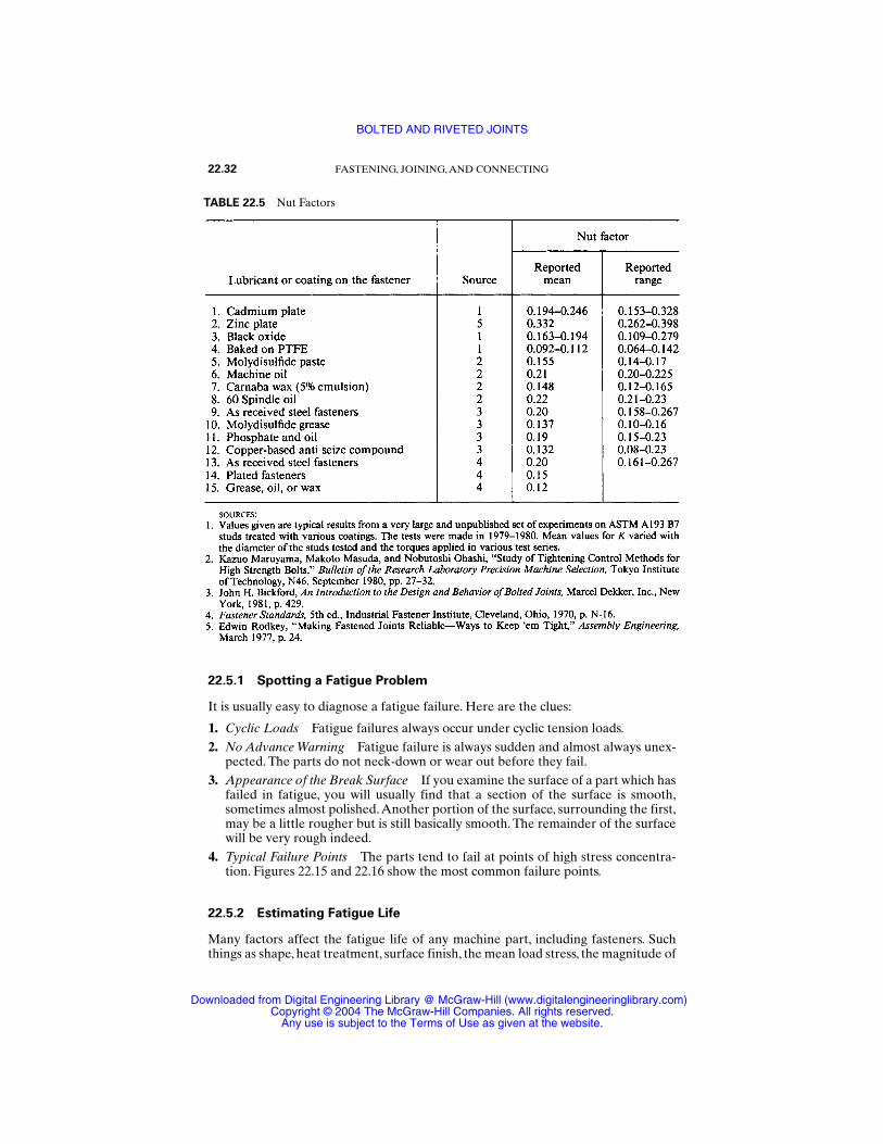
22.5.1 Spotting a Fatigue Problem
It is usually easy to diagnose a fatigue failure. Here are the clues:
1. Cyclic Loads Fatigue failures always occur under cyclic tension loads.2. No Advance Warning Fatigue failure is always sudden and almost always unex-
pected. The parts do not neck-down or wear out before they fail.3. Appearance of the Break Surface If you examine the surface of a part which has
failed in fatigue, you will usually find that a section of the surface is smooth,sometimes almost polished.Another portion of the surface, surrounding the first,may be a little rougher but is still basically smooth. The remainder of the surfacewill be very rough indeed.
4. Typical Failure Points The parts tend to fail at points of high stress concentra-tion. Figures 22.15 and 22.16 show the most common failure points.
22.5.2 Estimating Fatigue Life
Many factors affect the fatigue life of any machine part, including fasteners. Suchthings as shape, heat treatment, surface finish, the mean load stress, the magnitude of
22.32 FASTENING, JOINING, AND CONNECTING
TABLE 22.5 Nut Factors
BOLTED AND RIVETED JOINTS
Downloaded from Digital Engineering Library @ McGraw-Hill (www.digitalengineeringlibrary.com)Copyright © 2004 The McGraw-Hill Companies. All rights reserved.
Any use is subject to the Terms of Use as given at the website.
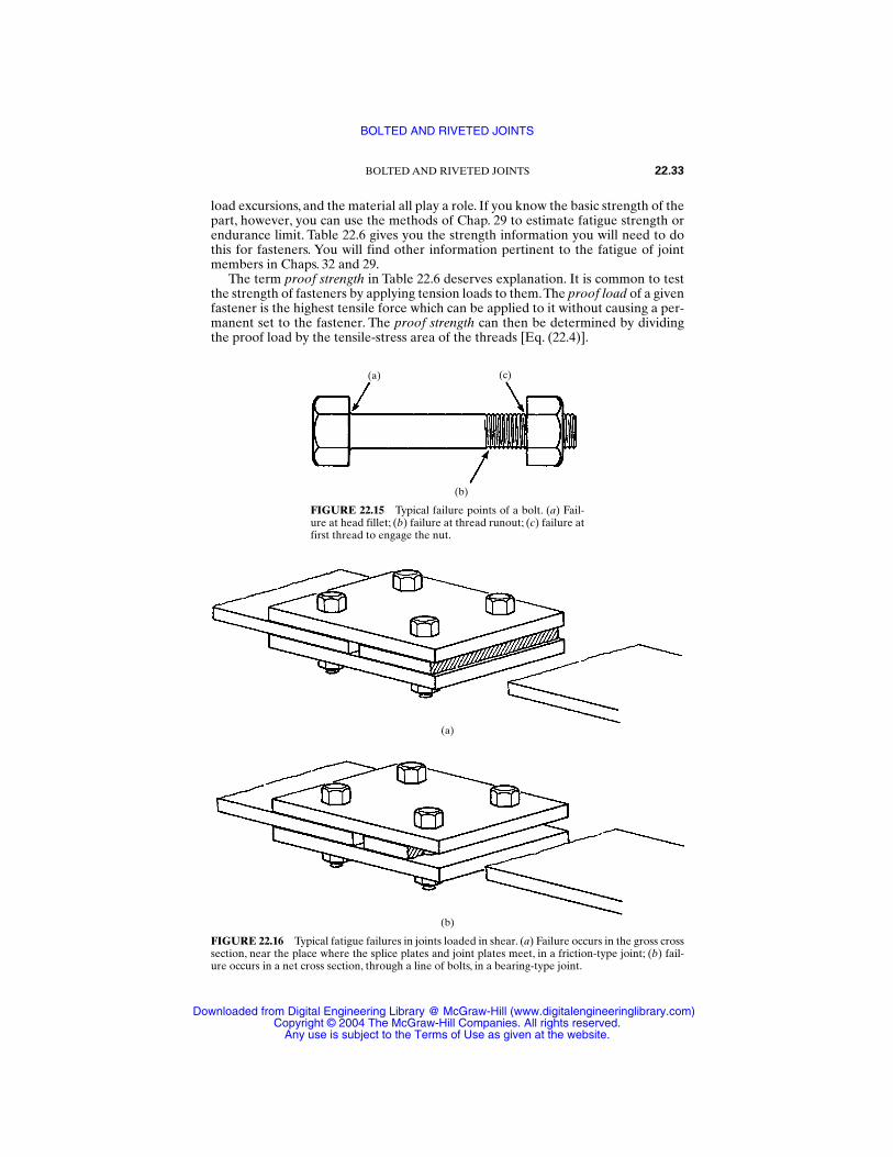
load excursions, and the material all play a role. If you know the basic strength of thepart, however, you can use the methods of Chap. 29 to estimate fatigue strength orendurance limit. Table 22.6 gives you the strength information you will need to dothis for fasteners. You will find other information pertinent to the fatigue of jointmembers in Chaps. 32 and 29.
The term proof strength in Table 22.6 deserves explanation. It is common to testthe strength of fasteners by applying tension loads to them.The proof load of a givenfastener is the highest tensile force which can be applied to it without causing a per-manent set to the fastener. The proof strength can then be determined by dividingthe proof load by the tensile-stress area of the threads [Eq. (22.4)].
BOLTED AND RIVETED JOINTS 22.33
FIGURE 22.15 Typical failure points of a bolt. (a) Fail-ure at head fillet; (b) failure at thread runout; (c) failure atfirst thread to engage the nut.
(a)
(b)
(c)
FIGURE 22.16 Typical fatigue failures in joints loaded in shear. (a) Failure occurs in the gross crosssection, near the place where the splice plates and joint plates meet, in a friction-type joint; (b) fail-ure occurs in a net cross section, through a line of bolts, in a bearing-type joint.
(a)
(b)
BOLTED AND RIVETED JOINTS
Downloaded from Digital Engineering Library @ McGraw-Hill (www.digitalengineeringlibrary.com)Copyright © 2004 The McGraw-Hill Companies. All rights reserved.
Any use is subject to the Terms of Use as given at the website.
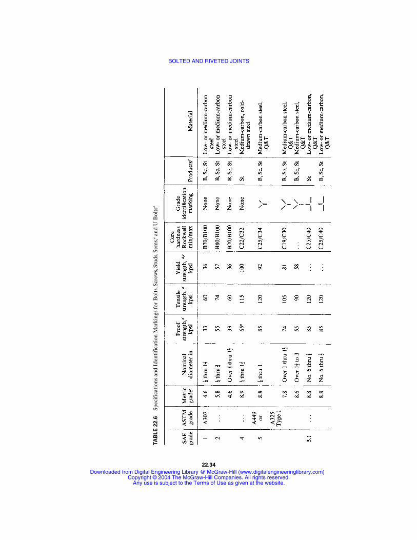
TA
BLE
22.6
Spec
ific
atio
ns a
nd I
dent
ific
atio
n M
arki
ngs
for
Bol
ts,S
crew
s,St
uds,
Sem
s,a
and
U B
olts
b
22.34
BOLTED AND RIVETED JOINTS
Downloaded from Digital Engineering Library @ McGraw-Hill (www.digitalengineeringlibrary.com)Copyright © 2004 The McGraw-Hill Companies. All rights reserved.
Any use is subject to the Terms of Use as given at the website.
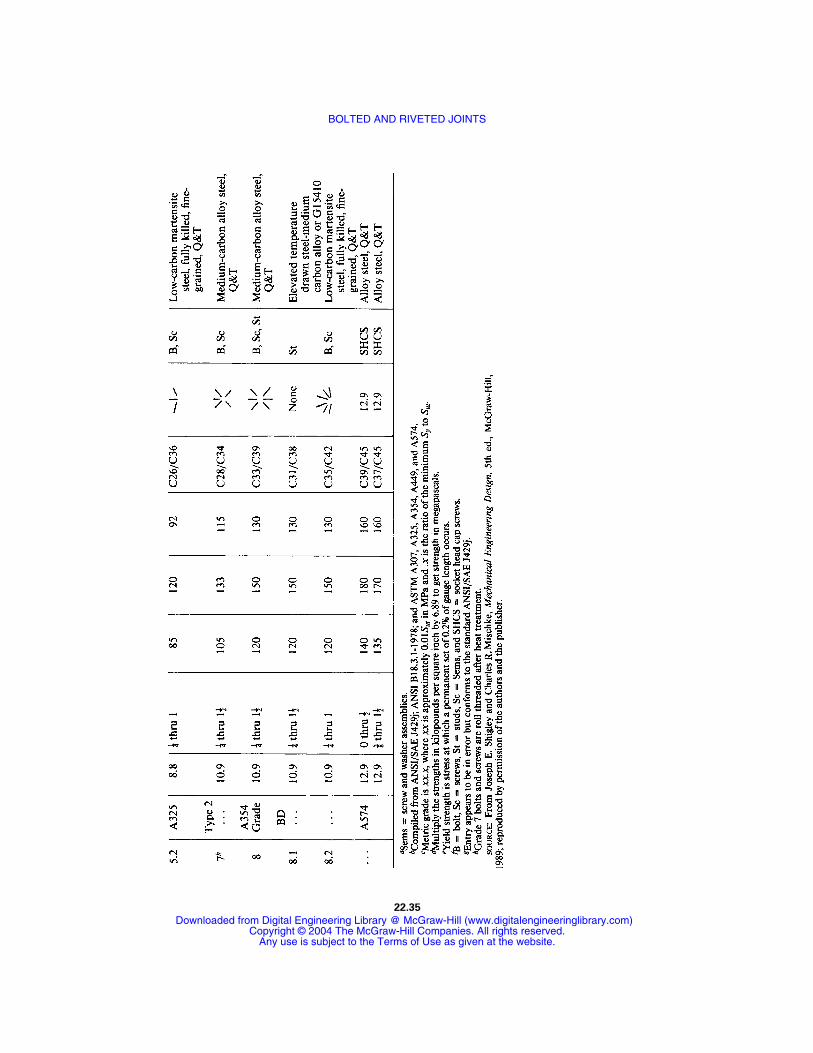
22.35
BOLTED AND RIVETED JOINTS
Downloaded from Digital Engineering Library @ McGraw-Hill (www.digitalengineeringlibrary.com)Copyright © 2004 The McGraw-Hill Companies. All rights reserved.
Any use is subject to the Terms of Use as given at the website.

22.5.3 Reducing Fatigue Problems
There are a lot of things you can do to minimize fatigue problems.
Material and Part Selection and Care. Materials with higher tensile strengthstend to have better fatigue lives than those with lower tensile strengths, at least up toan ultimate tensile strength of 200 kpsi (1379 MPa) or so. It also helps to select amaterial having low-notch sensitivity.
Avoid decarburization of the parts. Decarburization can weaken part surfacesand make it much easier for initial cracks to form.
Make sure that nut faces and the undersurface of the bolt head are perpendicu-lar to the axis of the bolt threads and that the holes are perpendicular to the surfacesof the joints [22.10].Two degrees of angularity can reduce fatigue life to only 25 per-cent of normal.
Lubricate the threads [22.10]. If nothing else, this can reduce corrosion problems,and corrosion is a main source of initial cracks.
If using fasteners with a tensile strength above 150 kpsi (1034 MPa), do not uselubricants containing sulfides, since these can contribute to stress-corrosion crack-ing, which will accelerate fatigue failure [22.11].
Grit blast the surfaces of joints loaded in shear before assembling because any-thing which increases the slip resistance improves fatigue life ([22.2], p. 120).
Prevent Crack Initiation. Polish, but do not hard coat, bolt surfaces, or shot peenthe surfaces, or roll bolt threads after heat treatment. Do anything and everythingpossible to avoid corrosion of bolts or joint members (see Chap. 35).
Reduce Load Excursions. Even if the magnitude of external loads imposed on ajoint are beyond the designer’s control, there are many things which he or she can doto reduce the variations in load seen by a given joint. And these variations, or loadexcursions, are a key issue.We always want to keep the ratio between minimum loadand maximum load seen by the parts as close to unity as possible.
Some say the minimum bolt tension should always be more than half the maxi-mum bolt tension. Others recommend a preload that is at least two to three timesthe magnitude of the worst-case external load to be applied to the joint. Because ofthe large number of variables involved, such rules will apply only to certain applica-tions. Nevertheless, they give you an idea of the importance of minimizing loadexcursions.
It helps to increase the ratio between the stiffness of the joint and the stiffness ofthe bolt (kJ/kB) so that the joint will absorb a larger percentage of the applied loadexcursions. There are many ways to do this. For examples, see Fig. 22.17a and b.Reducing the body of the bolt to nine-tenths of the nominal diameter is sometimesrecommended.
It helps to compensate for initial preload loss and relaxation effects by retighten-ing the bolts after they have relaxed. By the same token, try to avoid vibration lossof preload by providing damping and/or by periodic retightening of the nuts and/orby using special vibration-resistant fasteners.
Reduce Stresses in Parts. Make sure there are at least three threads above andbelow the faces of the nut (Fig. 22.17c). Do not let the thread run-out point coincidewith the shear plane of the joint (Fig. 22.17d). Roll the threads instead of cutting
22.36 FASTENING, JOINING, AND CONNECTING
BOLTED AND RIVETED JOINTS
Downloaded from Digital Engineering Library @ McGraw-Hill (www.digitalengineeringlibrary.com)Copyright © 2004 The McGraw-Hill Companies. All rights reserved.
Any use is subject to the Terms of Use as given at the website.
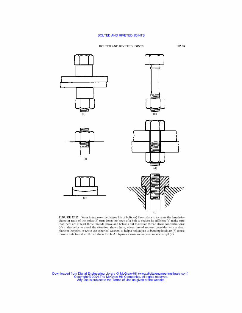
BOLTED AND RIVETED JOINTS 22.37
FIGURE 22.17 Ways to improve the fatigue life of bolts. (a) Use collars to increase the length-to-diameter ratio of the bolts; (b) turn down the body of a bolt to reduce its stiffness; (c) make surethat there are at least three threads above and below a nut to reduce thread stress concentrations;(d) it also helps to avoid the situation, shown here, where thread run-out coincides with a shearplane in the joint, or (e) to use spherical washers to help a bolt adjust to bending loads, or (f ) to usetension nuts to reduce thread stress levels. All figures shown are improvements except (d).
(a)
(c)
(e)
(b)
(d)
(f)
BOLTED AND RIVETED JOINTS
Downloaded from Digital Engineering Library @ McGraw-Hill (www.digitalengineeringlibrary.com)Copyright © 2004 The McGraw-Hill Companies. All rights reserved.
Any use is subject to the Terms of Use as given at the website.
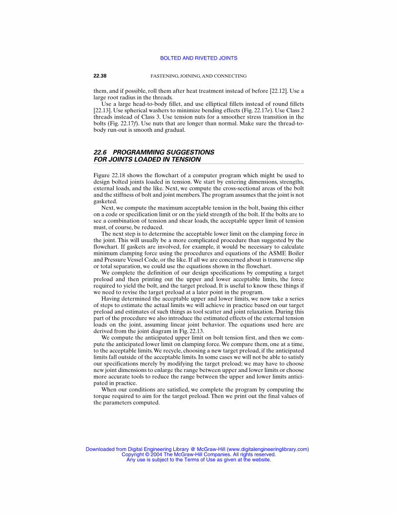
them, and if possible, roll them after heat treatment instead of before [22.12]. Use alarge root radius in the threads.
Use a large head-to-body fillet, and use elliptical fillets instead of round fillets[22.13]. Use spherical washers to minimize bending effects (Fig. 22.17e). Use Class 2threads instead of Class 3. Use tension nuts for a smoother stress transition in thebolts (Fig. 22.17f). Use nuts that are longer than normal. Make sure the thread-to-body run-out is smooth and gradual.
22.6 PROGRAMMING SUGGESTIONS FOR JOINTS LOADED IN TENSION
Figure 22.18 shows the flowchart of a computer program which might be used todesign bolted joints loaded in tension. We start by entering dimensions, strengths,external loads, and the like. Next, we compute the cross-sectional areas of the boltand the stiffness of bolt and joint members.The program assumes that the joint is notgasketed.
Next, we compute the maximum acceptable tension in the bolt, basing this eitheron a code or specification limit or on the yield strength of the bolt. If the bolts are tosee a combination of tension and shear loads, the acceptable upper limit of tensionmust, of course, be reduced.
The next step is to determine the acceptable lower limit on the clamping force inthe joint. This will usually be a more complicated procedure than suggested by theflowchart. If gaskets are involved, for example, it would be necessary to calculateminimum clamping force using the procedures and equations of the ASME Boilerand Pressure Vessel Code, or the like. If all we are concerned about is transverse slipor total separation, we could use the equations shown in the flowchart.
We complete the definition of our design specifications by computing a targetpreload and then printing out the upper and lower acceptable limits, the forcerequired to yield the bolt, and the target preload. It is useful to know these things ifwe need to revise the target preload at a later point in the program.
Having determined the acceptable upper and lower limits, we now take a seriesof steps to estimate the actual limits we will achieve in practice based on our targetpreload and estimates of such things as tool scatter and joint relaxation. During thispart of the procedure we also introduce the estimated effects of the external tensionloads on the joint, assuming linear joint behavior. The equations used here arederived from the joint diagram in Fig. 22.13.
We compute the anticipated upper limit on bolt tension first, and then we com-pute the anticipated lower limit on clamping force.We compare them, one at a time,to the acceptable limits.We recycle, choosing a new target preload, if the anticipatedlimits fall outside of the acceptable limits. In some cases we will not be able to satisfyour specifications merely by modifying the target preload; we may have to choosenew joint dimensions to enlarge the range between upper and lower limits or choosemore accurate tools to reduce the range between the upper and lower limits antici-pated in practice.
When our conditions are satisfied, we complete the program by computing thetorque required to aim for the target preload. Then we print out the final values ofthe parameters computed.
22.38 FASTENING, JOINING, AND CONNECTING
BOLTED AND RIVETED JOINTS
Downloaded from Digital Engineering Library @ McGraw-Hill (www.digitalengineeringlibrary.com)Copyright © 2004 The McGraw-Hill Companies. All rights reserved.
Any use is subject to the Terms of Use as given at the website.
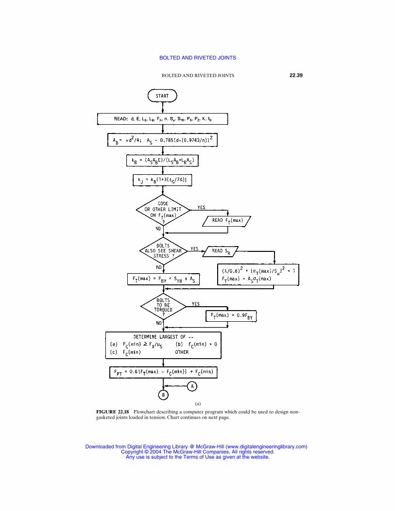
BOLTED AND RIVETED JOINTS 22.39
FIGURE 22.18 Flowchart describing a computer program which could be used to design non-gasketed joints loaded in tension. Chart continues on next page.
(a)
BOLTED AND RIVETED JOINTS
Downloaded from Digital Engineering Library @ McGraw-Hill (www.digitalengineeringlibrary.com)Copyright © 2004 The McGraw-Hill Companies. All rights reserved.
Any use is subject to the Terms of Use as given at the website.
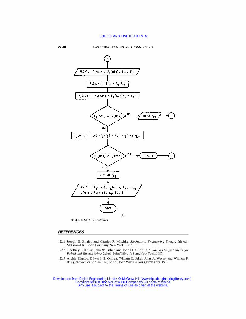
REFERENCES
22.1 Joseph E. Shigley and Charles R. Mischke, Mechanical Engineering Design, 5th ed.,McGraw-Hill Book Company, New York, 1989.
22.2 Goeffrey L. Kulak, John W. Fisher, and John H. A. Struik, Guide to Design Criteria forBolted and Riveted Joints, 2d ed., John Wiley & Sons, New York, 1987.
22.3 Archie Higdon, Edward H. Ohlsen, William B. Stiles, John A. Weese, and William F.Riley, Mechanics of Materials, 3d ed., John Wiley & Sons, New York, 1978.
22.40 FASTENING, JOINING, AND CONNECTING
FIGURE 22.18 (Continued)
(b)
BOLTED AND RIVETED JOINTS
Downloaded from Digital Engineering Library @ McGraw-Hill (www.digitalengineeringlibrary.com)Copyright © 2004 The McGraw-Hill Companies. All rights reserved.
Any use is subject to the Terms of Use as given at the website.

22.4 ANSI Specification B1.1-1974, “Screw Threads,” American Society of Mechanical Engi-neers, New York, 1974, p. 80.
22.5 Specifications BS 3643: Part 2: 1981, “ISO Metric Screw Threads,” British StandardsInstitute, London, 1981, p. 10.
22.6 John H. Bickford, An Introduction to the Design and Behavior of Bolted Joints, 2d ed.,Marcel Dekker, New York, 1990, p. 106.
22.7 Nabil Motosh, “Determination of Joint Stiffness in Bolted Connections,” Trans. ASME,August 1976, p. 859.
22.8 G. H. Junker,“Principle of the Calculation of High Duty Bolted Joints: Interpretation ofVDI Directive 2230,” Unbrako Technical Thesis, SPS, Jenkintown, Pa., 1974, p. 8.
22.9 Carl C. Osgood, Fatigue Design, Wiley-Interscience, New York, 1970, p. 196.
22.10 Joseph Viglione, “Nut Design Factors for Long Life,” Machine Design, August 1965, p.138.
22.11 “Degradation of Threaded Fasteners in the Reactor Coolant Pressure Boundary ofPWR Plants,” U.S. Nuclear Regulatory Commission, Washington, D.C., June 1982, p. 2.
22.12 Edwin Rodkey, “Making Fastened Joints Reliable—Ways to Keep ’em Tight,” AssemblyEngineering, March 1977, pp. 24–27.
22.13 “Thread Forms and Torque Systems Boost Reliability of Bolted Joints,” Product Engi-neering, December 1977, p. 38.
BOLTED AND RIVETED JOINTS 22.41
BOLTED AND RIVETED JOINTS
Downloaded from Digital Engineering Library @ McGraw-Hill (www.digitalengineeringlibrary.com)Copyright © 2004 The McGraw-Hill Companies. All rights reserved.
Any use is subject to the Terms of Use as given at the website.

BOLTED AND RIVETED JOINTS
Downloaded from Digital Engineering Library @ McGraw-Hill (www.digitalengineeringlibrary.com)Copyright © 2004 The McGraw-Hill Companies. All rights reserved.
Any use is subject to the Terms of Use as given at the website.
CHAPTER 23THREADED FASTENERS
Joseph E. ShigleyProfessor Emeritus
The University of MichiganAnn Arbor, Michigan
23.1 SCREW THREADS / 23.1
23.2 BOLTS / 23.5
23.3 SCREWS / 23.11
23.4 NUTS / 23.28
23.5 TAPPING SCREWS / 23.35
REFERENCE / 23.38
This chapter is intended to cover the description, uses, materials, and sizes ofthreaded fasteners. The amount of data available concerning this subject isextremely large, so the intent here is to provide the information necessary for theusual machine-design task of selecting such fasteners. The data contained in thischapter have been compiled in part from the standards listed in Ref. [23.1].
23.1 SCREW THREADS
Standard screw threads consist of the Unified inch series and the metric series. Twoprofiles have been standardized in the metric series; these are called the M and MJprofiles. Figure 23.1 shows that both the Unified and metric M threads utilize thesame profile.
The metric MJ profile has a rounded fillet at the root of the external thread anda larger minor diameter of both the internal and external threads.This profile is usedfor applications requiring a high fatigue strength and is also employed in aerospaceapplications.
The Unified-series profile, shown in Fig. 23.1, is designated as UN. Another uni-fied profile, designated as UNR, has a rounded root on the external thread.
Unified thread standards are based on the nominal size (major diameter) and thenumber of threads per inch. The three standards coarse (UNC), fine (UNF), andextra fine (UNEF) are listed in Table 23.1 and are called the standard series. Typicalspecifications would be written
1⁄4–20 UNC or 1⁄4–20 UNRC
Both these designations specify a nominal size of 1⁄4 in and 20 threads per inch.A constant-pitch unified series consisting of 4, 6, 8, 12, 16, 20, 28, and 32 threads
per inch has also been standardized. These are used mostly for sizes over 1 in, and 8UN, 12 UN, and 16 UN are the preferred pitches.
23.1
Source: STANDARD HANDBOOK OF MACHINE DESIGN
Downloaded from Digital Engineering Library @ McGraw-Hill (www.digitalengineeringlibrary.com)Copyright © 2004 The McGraw-Hill Companies. All rights reserved.
Any use is subject to the Terms of Use as given at the website.
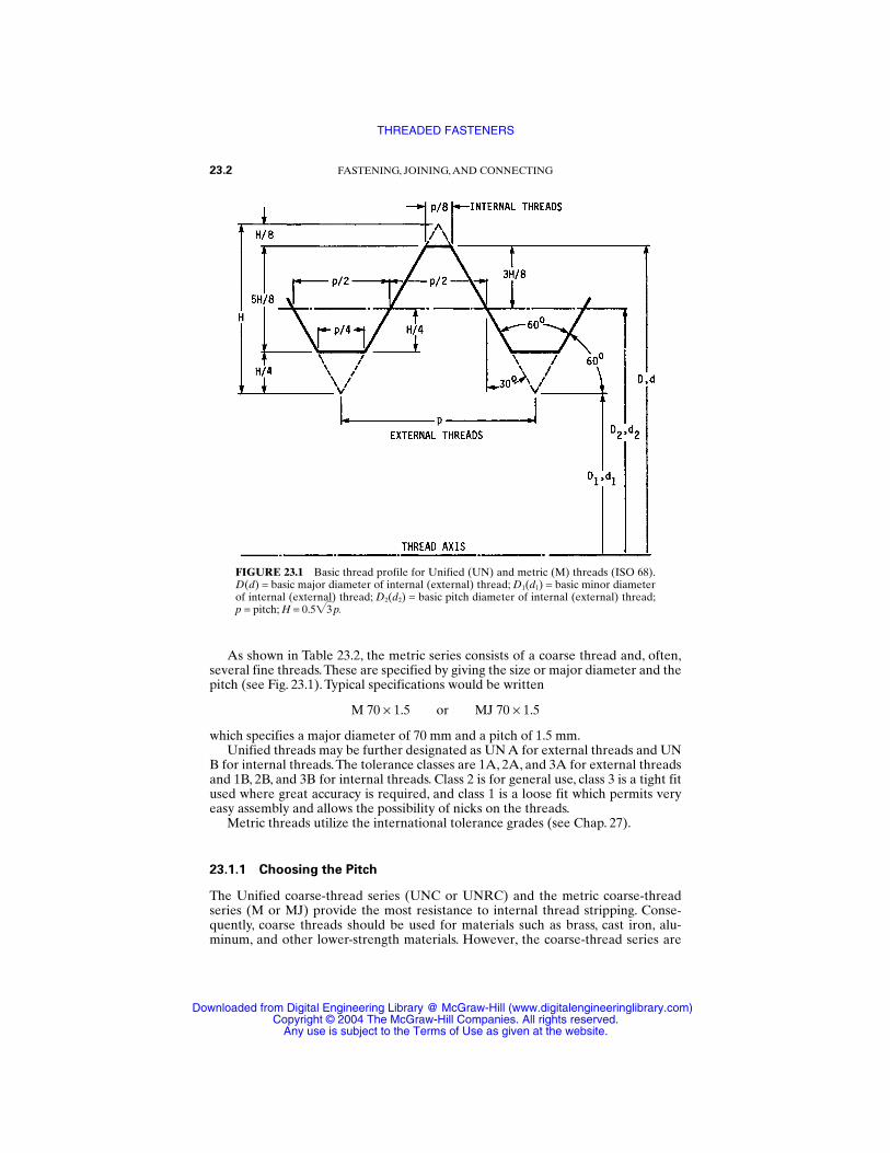
As shown in Table 23.2, the metric series consists of a coarse thread and, often,several fine threads.These are specified by giving the size or major diameter and thepitch (see Fig. 23.1). Typical specifications would be written
M 70 × 1.5 or MJ 70 × 1.5
which specifies a major diameter of 70 mm and a pitch of 1.5 mm.Unified threads may be further designated as UN A for external threads and UN
B for internal threads.The tolerance classes are 1A, 2A, and 3A for external threadsand 1B, 2B, and 3B for internal threads. Class 2 is for general use, class 3 is a tight fitused where great accuracy is required, and class 1 is a loose fit which permits veryeasy assembly and allows the possibility of nicks on the threads.
Metric threads utilize the international tolerance grades (see Chap. 27).
23.1.1 Choosing the Pitch
The Unified coarse-thread series (UNC or UNRC) and the metric coarse-threadseries (M or MJ) provide the most resistance to internal thread stripping. Conse-quently, coarse threads should be used for materials such as brass, cast iron, alu-minum, and other lower-strength materials. However, the coarse-thread series are
23.2 FASTENING, JOINING, AND CONNECTING
FIGURE 23.1 Basic thread profile for Unified (UN) and metric (M) threads (ISO 68).D(d) = basic major diameter of internal (external) thread; D1(d1) = basic minor diameterof internal (external) thread; D2(d2) = basic pitch diameter of internal (external) thread;p = pitch; H = 0.53 p.
THREADED FASTENERS
Downloaded from Digital Engineering Library @ McGraw-Hill (www.digitalengineeringlibrary.com)Copyright © 2004 The McGraw-Hill Companies. All rights reserved.
Any use is subject to the Terms of Use as given at the website.
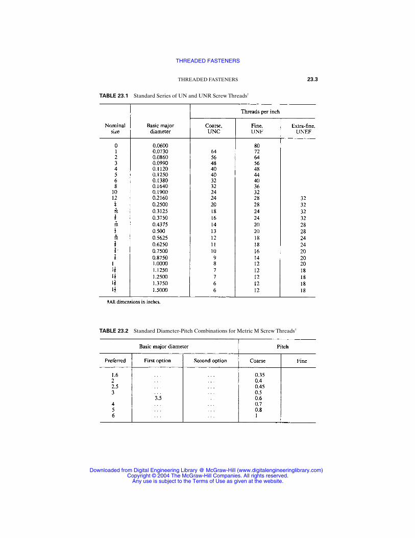
THREADED FASTENERS 23.3
TABLE 23.1 Standard Series of UN and UNR Screw Threads†
TABLE 23.2 Standard Diameter-Pitch Combinations for Metric M Screw Threads†
THREADED FASTENERS
Downloaded from Digital Engineering Library @ McGraw-Hill (www.digitalengineeringlibrary.com)Copyright © 2004 The McGraw-Hill Companies. All rights reserved.
Any use is subject to the Terms of Use as given at the website.
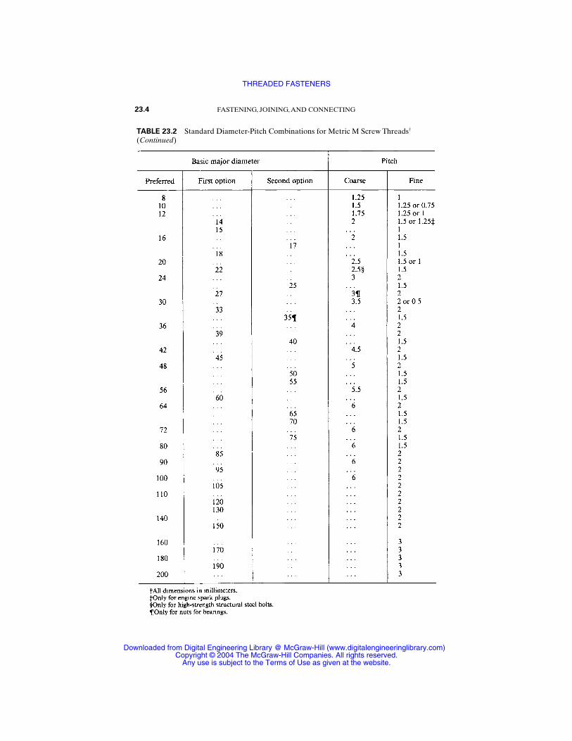
23.4 FASTENING, JOINING, AND CONNECTING
TABLE 23.2 Standard Diameter-Pitch Combinations for Metric M Screw Threads†
(Continued)
THREADED FASTENERS
Downloaded from Digital Engineering Library @ McGraw-Hill (www.digitalengineeringlibrary.com)Copyright © 2004 The McGraw-Hill Companies. All rights reserved.
Any use is subject to the Terms of Use as given at the website.
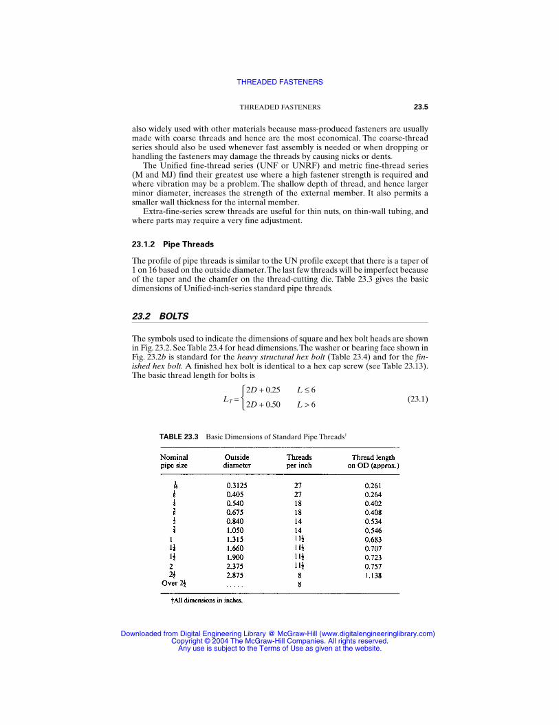
also widely used with other materials because mass-produced fasteners are usuallymade with coarse threads and hence are the most economical. The coarse-threadseries should also be used whenever fast assembly is needed or when dropping orhandling the fasteners may damage the threads by causing nicks or dents.
The Unified fine-thread series (UNF or UNRF) and metric fine-thread series (M and MJ) find their greatest use where a high fastener strength is required andwhere vibration may be a problem. The shallow depth of thread, and hence largerminor diameter, increases the strength of the external member. It also permits asmaller wall thickness for the internal member.
Extra-fine-series screw threads are useful for thin nuts, on thin-wall tubing, andwhere parts may require a very fine adjustment.
23.1.2 Pipe Threads
The profile of pipe threads is similar to the UN profile except that there is a taper of1 on 16 based on the outside diameter.The last few threads will be imperfect becauseof the taper and the chamfer on the thread-cutting die. Table 23.3 gives the basicdimensions of Unified-inch-series standard pipe threads.
23.2 BOLTS
The symbols used to indicate the dimensions of square and hex bolt heads are shownin Fig. 23.2. See Table 23.4 for head dimensions.The washer or bearing face shown inFig. 23.2b is standard for the heavy structural hex bolt (Table 23.4) and for the fin-ished hex bolt. A finished hex bolt is identical to a hex cap screw (see Table 23.13).The basic thread length for bolts is
LT = 2D + 0.25 L ≤ 6
2D + 0.50 L > 6(23.1)
THREADED FASTENERS 23.5
TABLE 23.3 Basic Dimensions of Standard Pipe Threads†
THREADED FASTENERS
Downloaded from Digital Engineering Library @ McGraw-Hill (www.digitalengineeringlibrary.com)Copyright © 2004 The McGraw-Hill Companies. All rights reserved.
Any use is subject to the Terms of Use as given at the website.
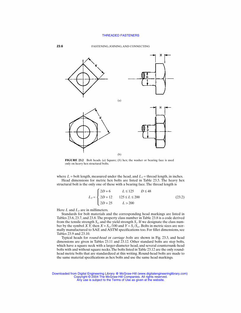
where L = bolt length, measured under the head, and LT = thread length, in inches.Head dimensions for metric hex bolts are listed in Table 23.5. The heavy hex
structural bolt is the only one of these with a bearing face. The thread length is
2D + 6 L ≤ 125 D ≤ 48
LT = 2D + 12 125 ≤ L ≤ 200 (23.2)
2D + 25 L > 200
Here L and LT are in millimeters.Standards for bolt materials and the corresponding head markings are listed in
Tables 23.6, 23.7, and 23.8. The property class number in Table 23.8 is a code derivedfrom the tensile strength Sut and the yield strength Sy. If we designate the class num-ber by the symbol X.Y, then X = Su t /100 and Y = Sy /Sut. Bolts in metric sizes are nor-mally manufactured to SAE and ASTM specifications too. For fillet dimensions, seeTables 23.9 and 23.10.
Typical heads for round-head or carriage bolts are shown in Fig. 23.3, and headdimensions are given in Tables 23.11 and 23.12. Other standard bolts are step bolts,which have a square neck with a larger-diameter head, and several countersunk-headbolts with and without square necks.The bolts listed in Table 23.12 are the only round-head metric bolts that are standardized at this writing. Round-head bolts are made tothe same material specifications as hex bolts and use the same head markings.
23.6 FASTENING, JOINING, AND CONNECTING
FIGURE 23.2 Bolt heads. (a) Square; (b) hex; the washer or bearing face is usedonly on heavy hex structural bolts.
(a)
(b)
THREADED FASTENERS
Downloaded from Digital Engineering Library @ McGraw-Hill (www.digitalengineeringlibrary.com)Copyright © 2004 The McGraw-Hill Companies. All rights reserved.
Any use is subject to the Terms of Use as given at the website.
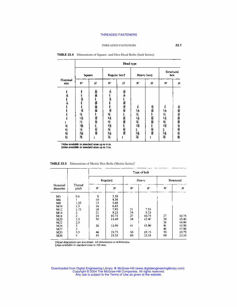
THREADED FASTENERS 23.7
TABLE 23.4 Dimensions of Square- and Hex-Head Bolts (Inch Series)
TABLE 23.5 Dimensions of Metric Hex Bolts (Metric Series)†
THREADED FASTENERS
Downloaded from Digital Engineering Library @ McGraw-Hill (www.digitalengineeringlibrary.com)Copyright © 2004 The McGraw-Hill Companies. All rights reserved.
Any use is subject to the Terms of Use as given at the website.
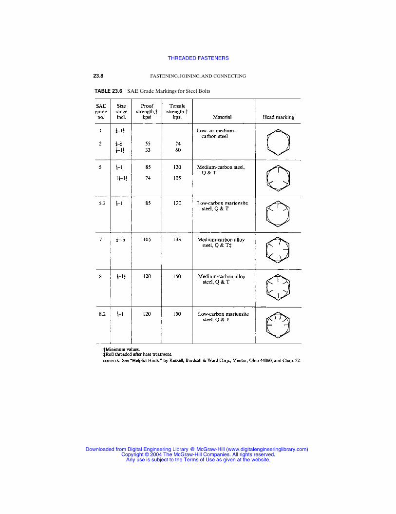
23.8 FASTENING, JOINING, AND CONNECTING
TABLE 23.6 SAE Grade Markings for Steel Bolts
THREADED FASTENERS
Downloaded from Digital Engineering Library @ McGraw-Hill (www.digitalengineeringlibrary.com)Copyright © 2004 The McGraw-Hill Companies. All rights reserved.
Any use is subject to the Terms of Use as given at the website.

THREADED FASTENERS 23.9
TABLE 23.7 ASTM Grade Markings for Steel Bolts
THREADED FASTENERS
Downloaded from Digital Engineering Library @ McGraw-Hill (www.digitalengineeringlibrary.com)Copyright © 2004 The McGraw-Hill Companies. All rights reserved.
Any use is subject to the Terms of Use as given at the website.

23.10 FASTENING, JOINING, AND CONNECTING
TABLE 23.8 Metric Mechanical-Property Classes for Steel Bolts, Screws, and Studs
THREADED FASTENERS
Downloaded from Digital Engineering Library @ McGraw-Hill (www.digitalengineeringlibrary.com)Copyright © 2004 The McGraw-Hill Companies. All rights reserved.
Any use is subject to the Terms of Use as given at the website.
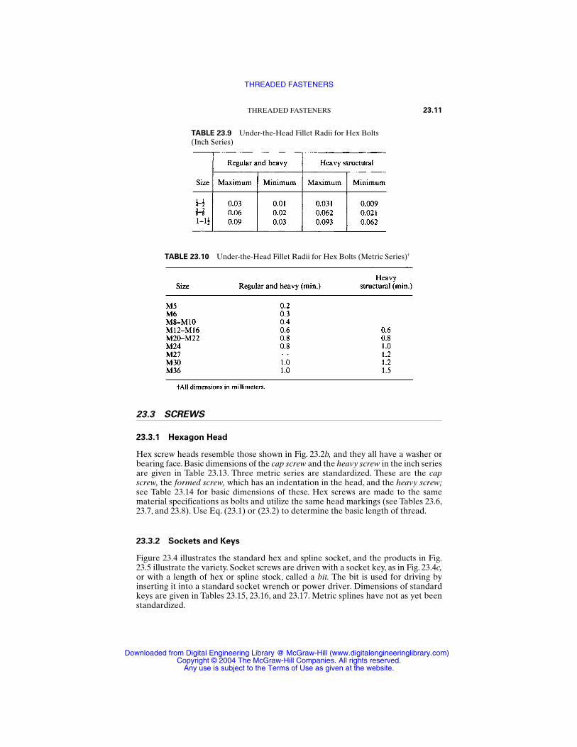
23.3 SCREWS
23.3.1 Hexagon Head
Hex screw heads resemble those shown in Fig. 23.2b, and they all have a washer orbearing face. Basic dimensions of the cap screw and the heavy screw in the inch seriesare given in Table 23.13. Three metric series are standardized. These are the capscrew, the formed screw, which has an indentation in the head, and the heavy screw;see Table 23.14 for basic dimensions of these. Hex screws are made to the samematerial specifications as bolts and utilize the same head markings (see Tables 23.6,23.7, and 23.8). Use Eq. (23.1) or (23.2) to determine the basic length of thread.
23.3.2 Sockets and Keys
Figure 23.4 illustrates the standard hex and spline socket, and the products in Fig.23.5 illustrate the variety. Socket screws are driven with a socket key, as in Fig. 23.4c,or with a length of hex or spline stock, called a bit. The bit is used for driving byinserting it into a standard socket wrench or power driver. Dimensions of standardkeys are given in Tables 23.15, 23.16, and 23.17. Metric splines have not as yet beenstandardized.
THREADED FASTENERS 23.11
TABLE 23.9 Under-the-Head Fillet Radii for Hex Bolts(Inch Series)
TABLE 23.10 Under-the-Head Fillet Radii for Hex Bolts (Metric Series)†
THREADED FASTENERS
Downloaded from Digital Engineering Library @ McGraw-Hill (www.digitalengineeringlibrary.com)Copyright © 2004 The McGraw-Hill Companies. All rights reserved.
Any use is subject to the Terms of Use as given at the website.
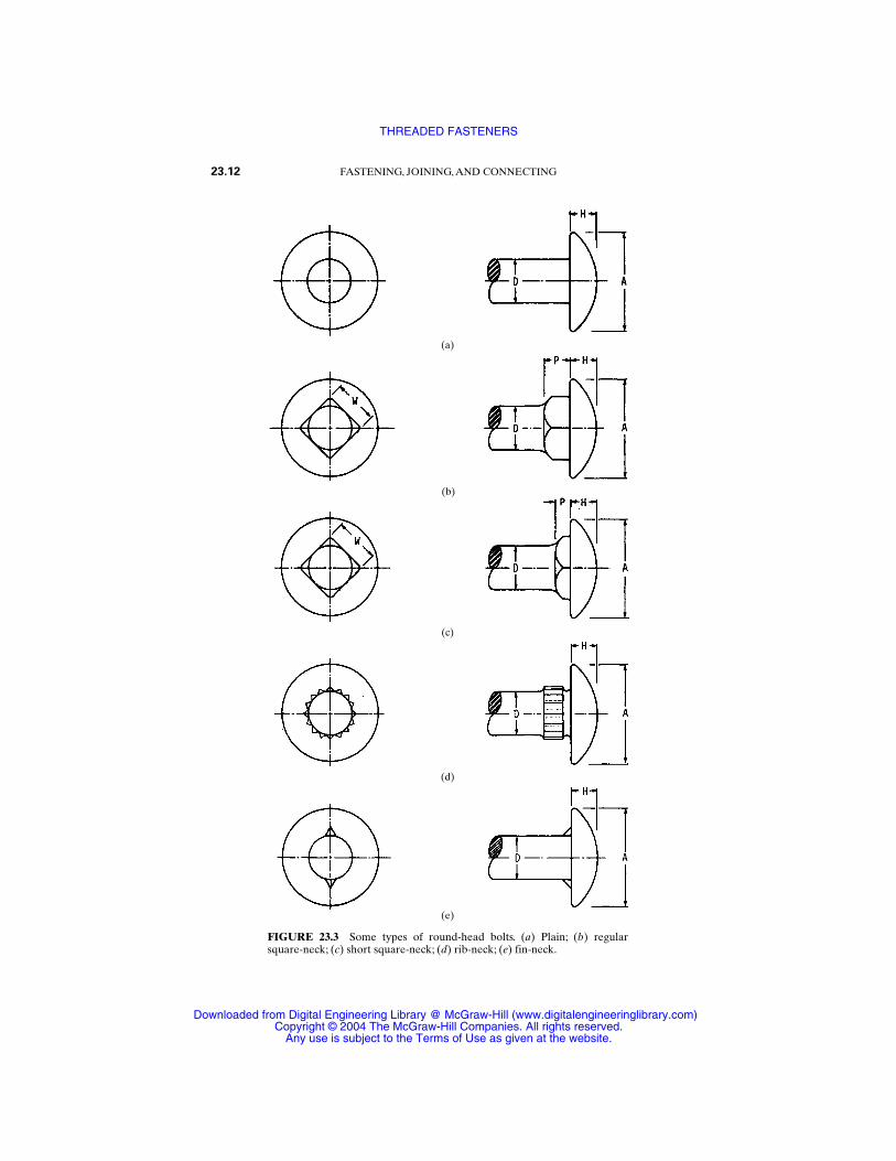
23.12 FASTENING, JOINING, AND CONNECTING
FIGURE 23.3 Some types of round-head bolts. (a) Plain; (b) regularsquare-neck; (c) short square-neck; (d) rib-neck; (e) fin-neck.
(e)
(d)
(c)
(b)
(a)
THREADED FASTENERS
Downloaded from Digital Engineering Library @ McGraw-Hill (www.digitalengineeringlibrary.com)Copyright © 2004 The McGraw-Hill Companies. All rights reserved.
Any use is subject to the Terms of Use as given at the website.

23.3.3 Socket-Head Cap Screws
Figure 23.6a illustrates a socket-head cap screw, and Fig. 23.6c shows a flat counter-sunk-head cap screw. Socket button-head cap screws resemble Fig. 23.8a, but have ahex or spline driving socket instead of the slot. Head dimensions for these, in inchand metric sizes, are given in Tables 23.18 to 23.23 inclusive.
Thread-length formulas are
LT = 2D + 0.50 in LT = 2D + 12 mm (23.3)
Shorter cap screws are threaded full length.Alloy-steel cap screws, in both inch and metric sizes, should contain an alloying
element, such as chromium, nickel, molybdenum, or vanadium, in such quantities asto ensure that a hardness range of 36 to 45 RC is achieved.
THREADED FASTENERS 23.13
TABLE 23.11 Some Basic Dimensions of Round-Head Bolts (Inch Series)†
TABLE 23.12 Some Basic Dimensions of Round-Head Short Square-Neck Metric Bolts
THREADED FASTENERS
Downloaded from Digital Engineering Library @ McGraw-Hill (www.digitalengineeringlibrary.com)Copyright © 2004 The McGraw-Hill Companies. All rights reserved.
Any use is subject to the Terms of Use as given at the website.
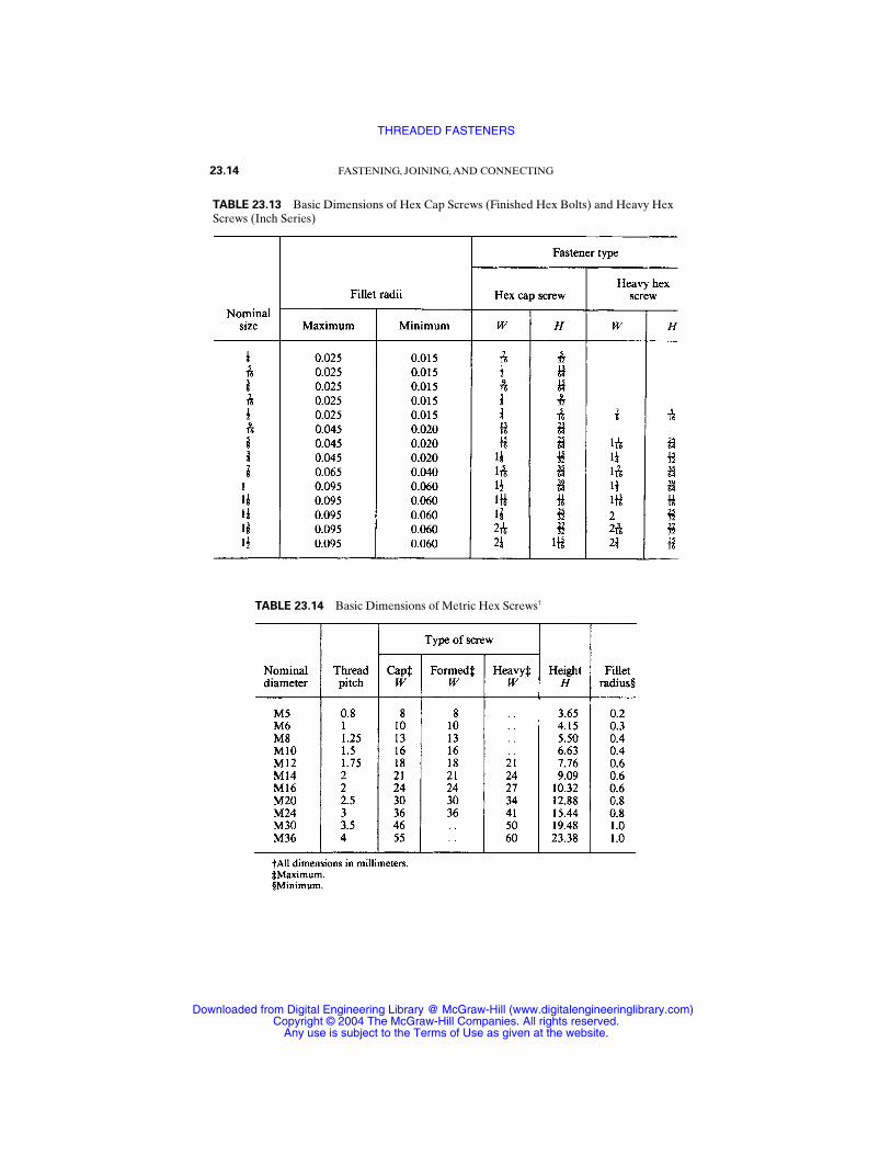
23.14 FASTENING, JOINING, AND CONNECTING
TABLE 23.13 Basic Dimensions of Hex Cap Screws (Finished Hex Bolts) and Heavy HexScrews (Inch Series)
TABLE 23.14 Basic Dimensions of Metric Hex Screws†
THREADED FASTENERS
Downloaded from Digital Engineering Library @ McGraw-Hill (www.digitalengineeringlibrary.com)Copyright © 2004 The McGraw-Hill Companies. All rights reserved.
Any use is subject to the Terms of Use as given at the website.
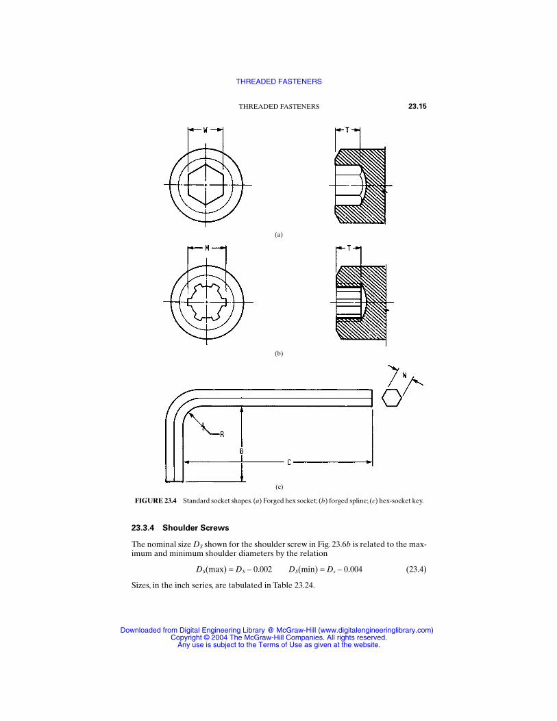
23.3.4 Shoulder Screws
The nominal size DS shown for the shoulder screw in Fig. 23.6b is related to the max-imum and minimum shoulder diameters by the relation
DS(max) = DS − 0.002 DS(min) = Ds − 0.004 (23.4)
Sizes, in the inch series, are tabulated in Table 23.24.
THREADED FASTENERS 23.15
FIGURE 23.4 Standard socket shapes. (a) Forged hex socket; (b) forged spline; (c) hex-socket key.
(c)
(b)
(a)
THREADED FASTENERS
Downloaded from Digital Engineering Library @ McGraw-Hill (www.digitalengineeringlibrary.com)Copyright © 2004 The McGraw-Hill Companies. All rights reserved.
Any use is subject to the Terms of Use as given at the website.
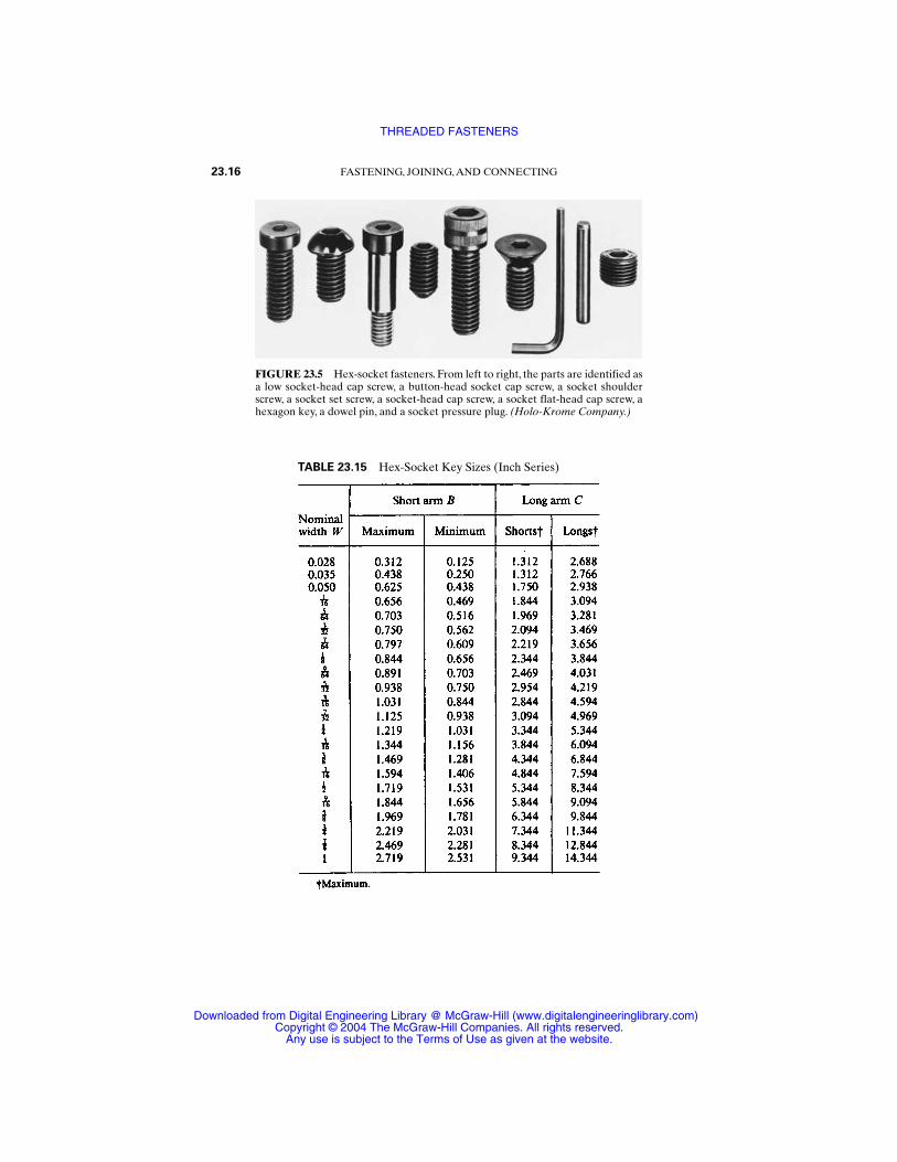
23.16 FASTENING, JOINING, AND CONNECTING
FIGURE 23.5 Hex-socket fasteners. From left to right, the parts are identified asa low socket-head cap screw, a button-head socket cap screw, a socket shoulderscrew, a socket set screw, a socket-head cap screw, a socket flat-head cap screw, ahexagon key, a dowel pin, and a socket pressure plug. (Holo-Krome Company.)
TABLE 23.15 Hex-Socket Key Sizes (Inch Series)
THREADED FASTENERS
Downloaded from Digital Engineering Library @ McGraw-Hill (www.digitalengineeringlibrary.com)Copyright © 2004 The McGraw-Hill Companies. All rights reserved.
Any use is subject to the Terms of Use as given at the website.

TABLE 23.16 Spline-Socket Key Sizes (Inch Series)
TABLE 23.17 Basic Maximum Dimensions of Metric Hex Keys†
23.17
THREADED FASTENERS
Downloaded from Digital Engineering Library @ McGraw-Hill (www.digitalengineeringlibrary.com)Copyright © 2004 The McGraw-Hill Companies. All rights reserved.
Any use is subject to the Terms of Use as given at the website.
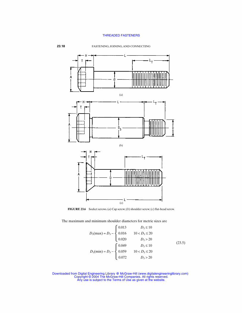
The maximum and minimum shoulder diameters for metric sizes are
0.013 DS ≤ 10
DS(max) = DS − 0.016 10 < DS ≤ 20
0.020 DS > 20(23.5)
0.049 DS ≤ 10
DS(min) = DS − 0.059 10 < DS ≤ 20
0.072 DS > 20
23.18 FASTENING, JOINING, AND CONNECTING
FIGURE 23.6 Socket screws. (a) Cap screw; (b) shoulder screw; (c) flat-head screw.
(a)
(b)
(c)
THREADED FASTENERS
Downloaded from Digital Engineering Library @ McGraw-Hill (www.digitalengineeringlibrary.com)Copyright © 2004 The McGraw-Hill Companies. All rights reserved.
Any use is subject to the Terms of Use as given at the website.
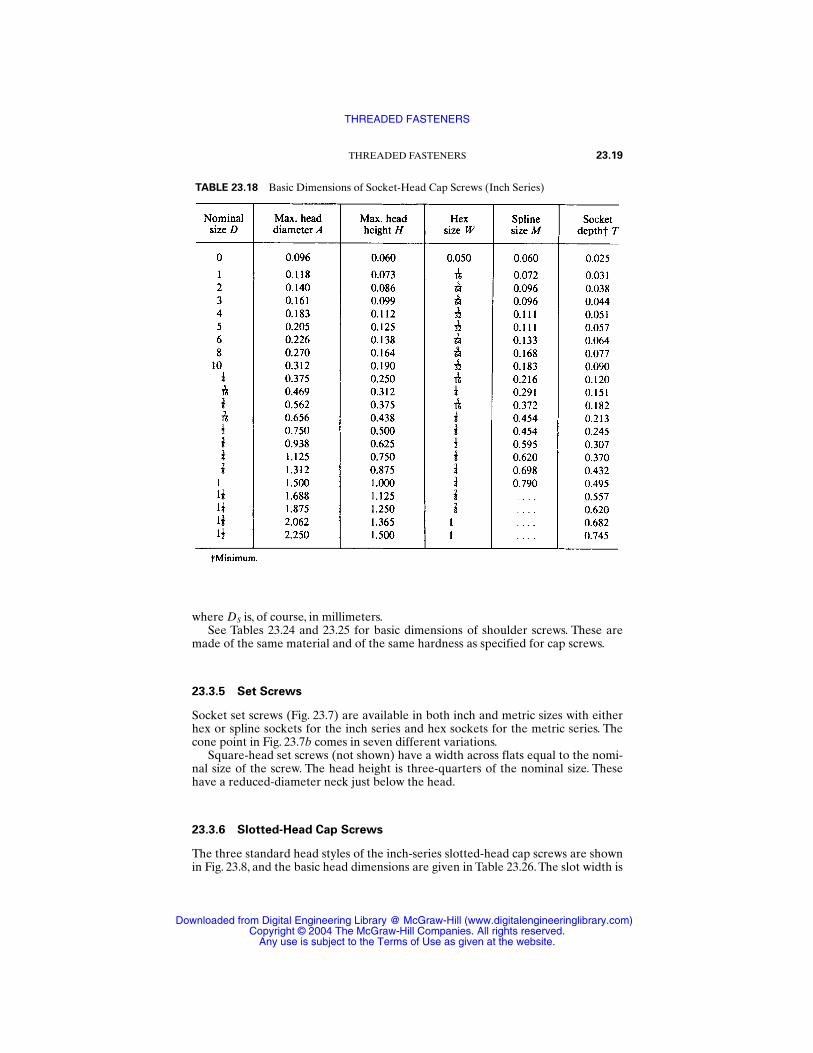
where DS is, of course, in millimeters.See Tables 23.24 and 23.25 for basic dimensions of shoulder screws. These are
made of the same material and of the same hardness as specified for cap screws.
23.3.5 Set Screws
Socket set screws (Fig. 23.7) are available in both inch and metric sizes with eitherhex or spline sockets for the inch series and hex sockets for the metric series. Thecone point in Fig. 23.7b comes in seven different variations.
Square-head set screws (not shown) have a width across flats equal to the nomi-nal size of the screw. The head height is three-quarters of the nominal size. Thesehave a reduced-diameter neck just below the head.
23.3.6 Slotted-Head Cap Screws
The three standard head styles of the inch-series slotted-head cap screws are shownin Fig. 23.8, and the basic head dimensions are given in Table 23.26. The slot width is
THREADED FASTENERS 23.19
TABLE 23.18 Basic Dimensions of Socket-Head Cap Screws (Inch Series)
THREADED FASTENERS
Downloaded from Digital Engineering Library @ McGraw-Hill (www.digitalengineeringlibrary.com)Copyright © 2004 The McGraw-Hill Companies. All rights reserved.
Any use is subject to the Terms of Use as given at the website.
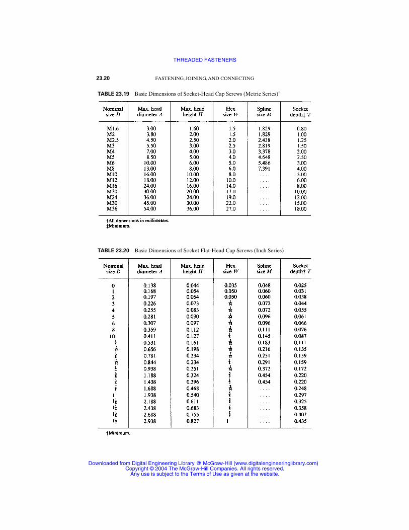
23.20 FASTENING, JOINING, AND CONNECTING
TABLE 23.19 Basic Dimensions of Socket-Head Cap Screws (Metric Series)†
TABLE 23.20 Basic Dimensions of Socket Flat-Head Cap Screws (Inch Series)
THREADED FASTENERS
Downloaded from Digital Engineering Library @ McGraw-Hill (www.digitalengineeringlibrary.com)Copyright © 2004 The McGraw-Hill Companies. All rights reserved.
Any use is subject to the Terms of Use as given at the website.

TABLE 23.21 Basic Dimensions of Socket Flat-Head Cap Screws (Metric Series)†
TABLE 23.22 Basic Dimensions of Socket Button-Head Cap Screws (Inch Series)
TABLE 23.23 Basic Dimensions of Socket Button-Head Cap Screws (Metric Series)†
23.21
THREADED FASTENERS
Downloaded from Digital Engineering Library @ McGraw-Hill (www.digitalengineeringlibrary.com)Copyright © 2004 The McGraw-Hill Companies. All rights reserved.
Any use is subject to the Terms of Use as given at the website.
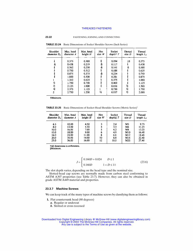
J = 0.160D + 0.024 D ≤ 1
0.160D 1 < D ≤ 11⁄2(23.6)
The slot depth varies, depending on the head type and the nominal size.Slotted-head cap screws are normally made from carbon steel conforming to
ASTM A307 properties (see Table 23.7). However, they can also be obtained ingrade ASTM A449 material and properties.
23.3.7 Machine Screws
We can keep track of the many types of machine screws by classifying them as follows:
1. Flat countersunk head (80 degrees)a. Regular or undercutb. Slotted or cross-recessed
23.22 FASTENING, JOINING, AND CONNECTING
TABLE 23.24 Basic Dimensions of Socket Shoulder Screws (Inch Series)
TABLE 23.25 Basic Dimensions of Socket-Head Shoulder Screws (Metric Series)†
THREADED FASTENERS
Downloaded from Digital Engineering Library @ McGraw-Hill (www.digitalengineeringlibrary.com)Copyright © 2004 The McGraw-Hill Companies. All rights reserved.
Any use is subject to the Terms of Use as given at the website.
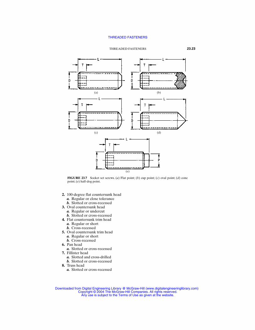
2. 100-degree flat countersunk heada. Regular or close toleranceb. Slotted or cross-recessed
3. Oval countersunk heada. Regular or undercutb. Slotted or cross-recessed
4. Flat countersunk trim heada. Regular or shortb. Cross-recessed
5. Oval countersunk trim heada. Regular or shortb. Cross-recessed
6. Pan heada. Slotted or cross-recessed
7. Fillister heada. Slotted and cross-drilledb. Slotted or cross-recessed
8. Truss heada. Slotted or cross-recessed
THREADED FASTENERS 23.23
FIGURE 23.7 Socket set screws. (a) Flat point; (b) cup point; (c) oval point; (d) conepoint; (e) half-dog point.
(a) (b)
(c) (d)
(e)
THREADED FASTENERS
Downloaded from Digital Engineering Library @ McGraw-Hill (www.digitalengineeringlibrary.com)Copyright © 2004 The McGraw-Hill Companies. All rights reserved.
Any use is subject to the Terms of Use as given at the website.
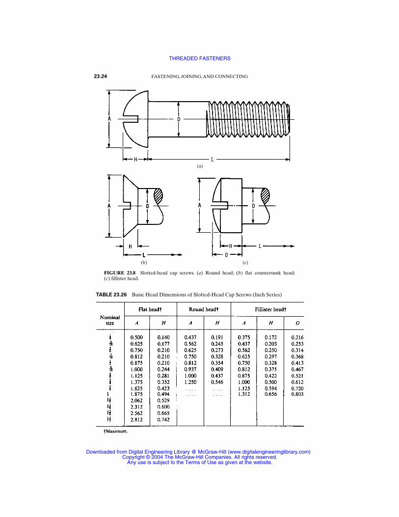
23.24 FASTENING, JOINING, AND CONNECTING
FIGURE 23.8 Slotted-head cap screws. (a) Round head; (b) flat countersunk head;(c) fillister head.
(a)
(b) (c)
TABLE 23.26 Basic Head Dimensions of Slotted-Head Cap Screws (Inch Series)
THREADED FASTENERS
Downloaded from Digital Engineering Library @ McGraw-Hill (www.digitalengineeringlibrary.com)Copyright © 2004 The McGraw-Hill Companies. All rights reserved.
Any use is subject to the Terms of Use as given at the website.
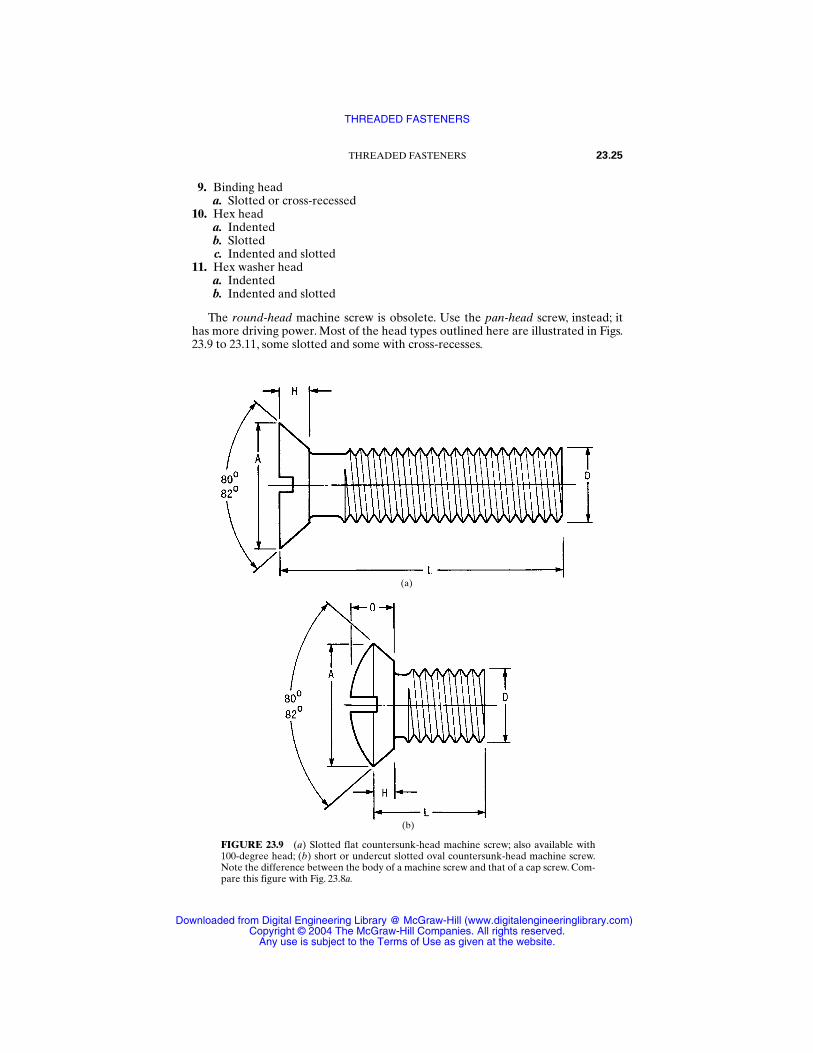
9. Binding heada. Slotted or cross-recessed
10. Hex heada. Indentedb. Slottedc. Indented and slotted
11. Hex washer heada. Indentedb. Indented and slotted
The round-head machine screw is obsolete. Use the pan-head screw, instead; ithas more driving power. Most of the head types outlined here are illustrated in Figs.23.9 to 23.11, some slotted and some with cross-recesses.
THREADED FASTENERS 23.25
FIGURE 23.9 (a) Slotted flat countersunk-head machine screw; also available with100-degree head; (b) short or undercut slotted oval countersunk-head machine screw.Note the difference between the body of a machine screw and that of a cap screw. Com-pare this figure with Fig. 23.8a.
(a)
(b)
THREADED FASTENERS
Downloaded from Digital Engineering Library @ McGraw-Hill (www.digitalengineeringlibrary.com)Copyright © 2004 The McGraw-Hill Companies. All rights reserved.
Any use is subject to the Terms of Use as given at the website.
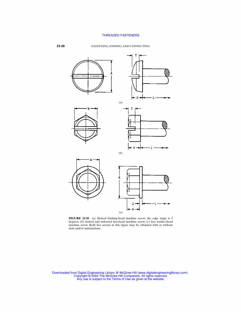
23.26 FASTENING, JOINING, AND CONNECTING
FIGURE 23.10 (a) Slotted binding-head machine screw; the edge angle is 5degrees; (b) slotted and indented hex-head machine screw; (c) hex washer-headmachine screw. Both hex screws in this figure may be obtained with or withoutslots and/or indentations.
(a)
(b)
(c)
THREADED FASTENERS
Downloaded from Digital Engineering Library @ McGraw-Hill (www.digitalengineeringlibrary.com)Copyright © 2004 The McGraw-Hill Companies. All rights reserved.
Any use is subject to the Terms of Use as given at the website.
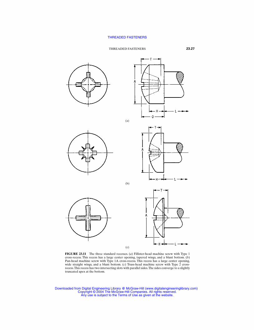
THREADED FASTENERS 23.27
FIGURE 23.11 The three standard recesses. (a) Fillister-head machine screw with Type 1cross-recess. This recess has a large center opening, tapered wings, and a blunt bottom. (b)Pan-head machine screw with Type 1A cross-recess. This recess has a large center opening,wide straight wings, and a blunt bottom. (c) Truss-head machine screw with Type 2 cross-recess.This recess has two intersecting slots with parallel sides.The sides converge to a slightlytruncated apex at the bottom.
(a)
(b)
(c)
THREADED FASTENERS
Downloaded from Digital Engineering Library @ McGraw-Hill (www.digitalengineeringlibrary.com)Copyright © 2004 The McGraw-Hill Companies. All rights reserved.
Any use is subject to the Terms of Use as given at the website.
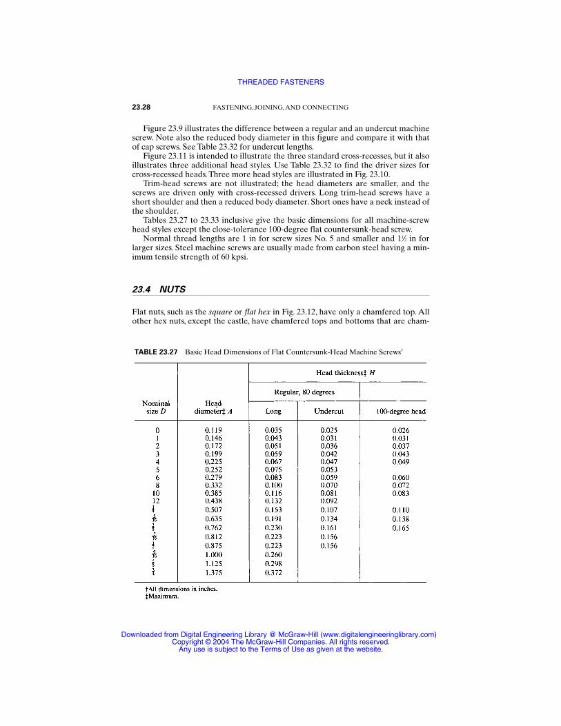
Figure 23.9 illustrates the difference between a regular and an undercut machinescrew. Note also the reduced body diameter in this figure and compare it with thatof cap screws. See Table 23.32 for undercut lengths.
Figure 23.11 is intended to illustrate the three standard cross-recesses, but it alsoillustrates three additional head styles. Use Table 23.32 to find the driver sizes forcross-recessed heads. Three more head styles are illustrated in Fig. 23.10.
Trim-head screws are not illustrated; the head diameters are smaller, and thescrews are driven only with cross-recessed drivers. Long trim-head screws have ashort shoulder and then a reduced body diameter. Short ones have a neck instead ofthe shoulder.
Tables 23.27 to 23.33 inclusive give the basic dimensions for all machine-screwhead styles except the close-tolerance 100-degree flat countersunk-head screw.
Normal thread lengths are 1 in for screw sizes No. 5 and smaller and 11⁄2 in forlarger sizes. Steel machine screws are usually made from carbon steel having a min-imum tensile strength of 60 kpsi.
23.4 NUTS
Flat nuts, such as the square or flat hex in Fig. 23.12, have only a chamfered top. Allother hex nuts, except the castle, have chamfered tops and bottoms that are cham-
23.28 FASTENING, JOINING, AND CONNECTING
TABLE 23.27 Basic Head Dimensions of Flat Countersunk-Head Machine Screws†
THREADED FASTENERS
Downloaded from Digital Engineering Library @ McGraw-Hill (www.digitalengineeringlibrary.com)Copyright © 2004 The McGraw-Hill Companies. All rights reserved.
Any use is subject to the Terms of Use as given at the website.

THREADED FASTENERS 23.29
TABLE 23.28 Total Head Heights O for Oval Countersunk-Head Machine Screws†
TABLE 23.29 Basic Head Dimensions of Flat and Oval Countersunk Trim-Head MachineScrews (Available Only with Cross-Recessed Heads)†
THREADED FASTENERS
Downloaded from Digital Engineering Library @ McGraw-Hill (www.digitalengineeringlibrary.com)Copyright © 2004 The McGraw-Hill Companies. All rights reserved.
Any use is subject to the Terms of Use as given at the website.
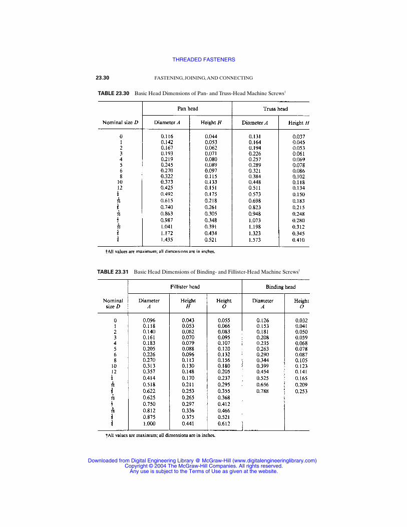
23.30 FASTENING, JOINING, AND CONNECTING
TABLE 23.30 Basic Head Dimensions of Pan- and Truss-Head Machine Screws†
TABLE 23.31 Basic Head Dimensions of Binding- and Fillister-Head Machine Screws†
THREADED FASTENERS
Downloaded from Digital Engineering Library @ McGraw-Hill (www.digitalengineeringlibrary.com)Copyright © 2004 The McGraw-Hill Companies. All rights reserved.
Any use is subject to the Terms of Use as given at the website.
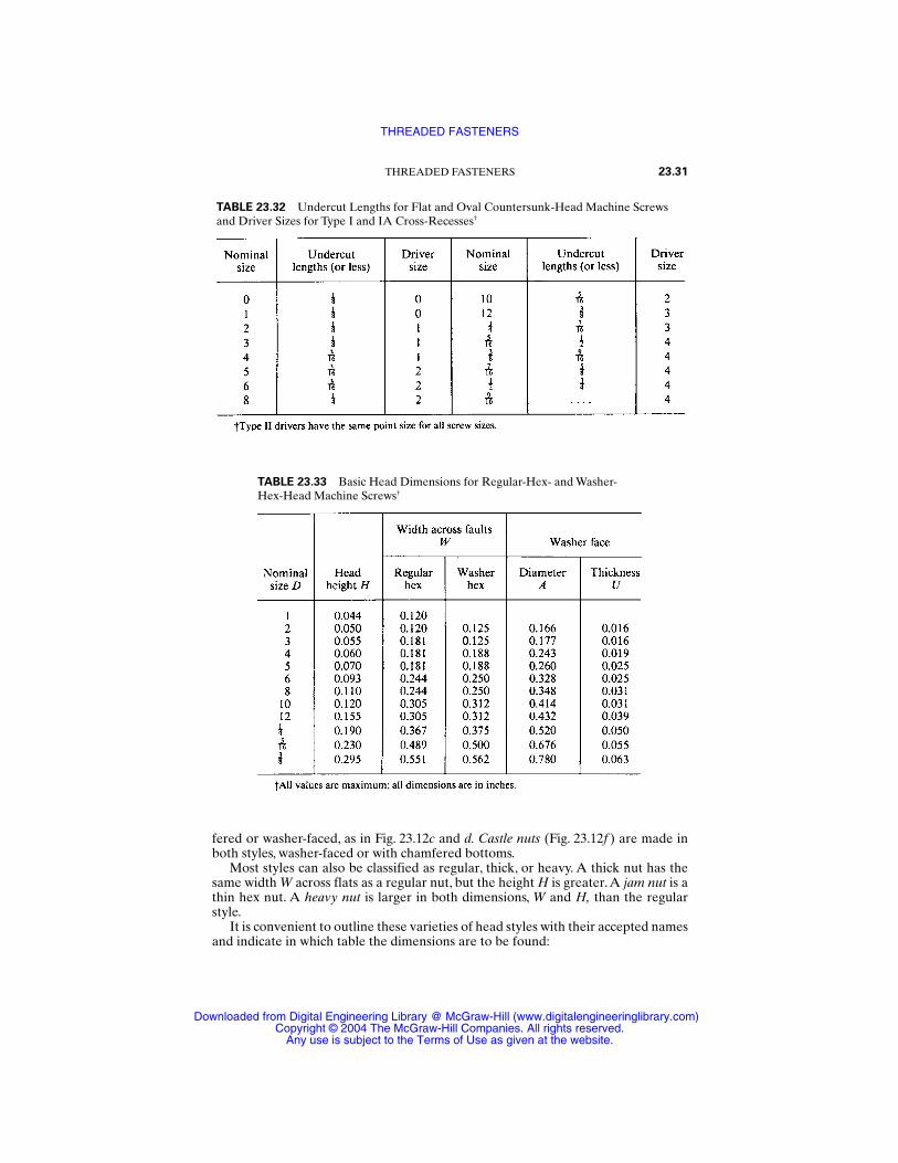
fered or washer-faced, as in Fig. 23.12c and d. Castle nuts (Fig. 23.12f ) are made inboth styles, washer-faced or with chamfered bottoms.
Most styles can also be classified as regular, thick, or heavy. A thick nut has thesame width W across flats as a regular nut, but the height H is greater.A jam nut is athin hex nut. A heavy nut is larger in both dimensions, W and H, than the regularstyle.
It is convenient to outline these varieties of head styles with their accepted namesand indicate in which table the dimensions are to be found:
THREADED FASTENERS 23.31
TABLE 23.32 Undercut Lengths for Flat and Oval Countersunk-Head Machine Screws and Driver Sizes for Type I and IA Cross-Recesses†
TABLE 23.33 Basic Head Dimensions for Regular-Hex- and Washer-Hex-Head Machine Screws†
THREADED FASTENERS
Downloaded from Digital Engineering Library @ McGraw-Hill (www.digitalengineeringlibrary.com)Copyright © 2004 The McGraw-Hill Companies. All rights reserved.
Any use is subject to the Terms of Use as given at the website.
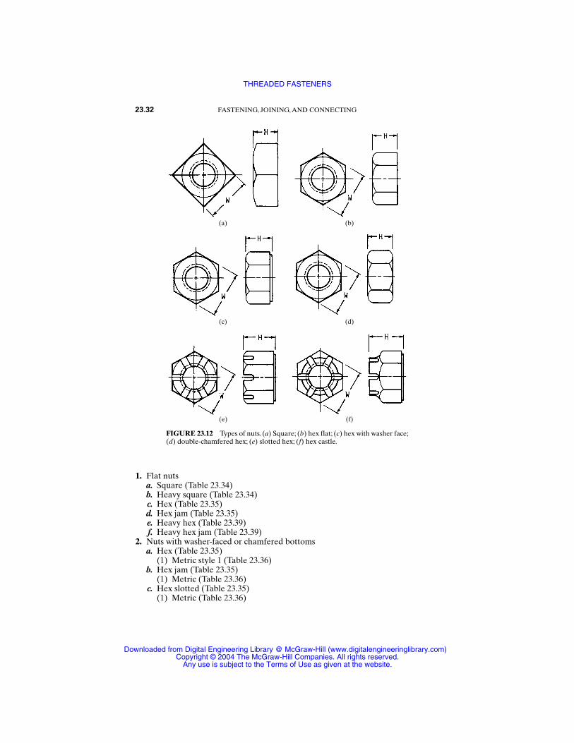
1. Flat nutsa. Square (Table 23.34)b. Heavy square (Table 23.34)c. Hex (Table 23.35)d. Hex jam (Table 23.35)e. Heavy hex (Table 23.39)f. Heavy hex jam (Table 23.39)
2. Nuts with washer-faced or chamfered bottomsa. Hex (Table 23.35)
(1) Metric style 1 (Table 23.36)b. Hex jam (Table 23.35)
(1) Metric (Table 23.36)c. Hex slotted (Table 23.35)
(1) Metric (Table 23.36)
23.32 FASTENING, JOINING, AND CONNECTING
FIGURE 23.12 Types of nuts. (a) Square; (b) hex flat; (c) hex with washer face;(d) double-chamfered hex; (e) slotted hex; (f) hex castle.
(a) (b)
(c) (d)
(e) (f)
THREADED FASTENERS
Downloaded from Digital Engineering Library @ McGraw-Hill (www.digitalengineeringlibrary.com)Copyright © 2004 The McGraw-Hill Companies. All rights reserved.
Any use is subject to the Terms of Use as given at the website.

THREADED FASTENERS 23.33
TABLE 23.34 Basic Dimensions of SquareNuts (Inch Series)
TABLE 23.35 Basic Dimensions of Hex, Hex Jam, Hex Flat, Hex Flat Jam, Hex Slotted,Hex Thick, and Hex Thick Slotted Nuts (Inch Series)
THREADED FASTENERS
Downloaded from Digital Engineering Library @ McGraw-Hill (www.digitalengineeringlibrary.com)Copyright © 2004 The McGraw-Hill Companies. All rights reserved.
Any use is subject to the Terms of Use as given at the website.
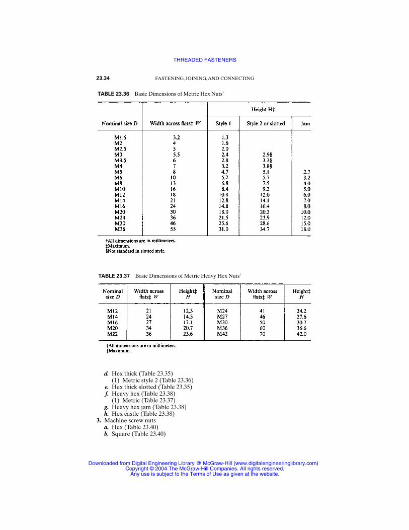
d. Hex thick (Table 23.35)(1) Metric style 2 (Table 23.36)
e. Hex thick slotted (Table 23.35)f. Heavy hex (Table 23.38)
(1) Metric (Table 23.37)g. Heavy hex jam (Table 23.38)h. Hex castle (Table 23.38)
3. Machine screw nutsa. Hex (Table 23.40)b. Square (Table 23.40)
23.34 FASTENING, JOINING, AND CONNECTING
TABLE 23.36 Basic Dimensions of Metric Hex Nuts†
TABLE 23.37 Basic Dimensions of Metric Heavy Hex Nuts†
THREADED FASTENERS
Downloaded from Digital Engineering Library @ McGraw-Hill (www.digitalengineeringlibrary.com)Copyright © 2004 The McGraw-Hill Companies. All rights reserved.
Any use is subject to the Terms of Use as given at the website.

Carbon steel nuts usually are made to conform to ASTM A563 Grade A specifi-cations or to SAE Grade 2.
23.5 TAPPING SCREWS
Self-tapping screws are available in all head styles and in sizes up to and including 3⁄8in. They are hardened sufficiently to form their own mating threads when driven. In
THREADED FASTENERS 23.35
TABLE 23.38 Basic Dimensions of Heavy Hex, Heavy Hex Jam, Heavy Hex Slotted, andHeavy Hex Castle Nuts (Inch Series)
TABLE 23.39 Basic Dimensions of HeavyHex Flat and Heavy Hex Flat Jam Nuts (Inch Series)
THREADED FASTENERS
Downloaded from Digital Engineering Library @ McGraw-Hill (www.digitalengineeringlibrary.com)Copyright © 2004 The McGraw-Hill Companies. All rights reserved.
Any use is subject to the Terms of Use as given at the website.
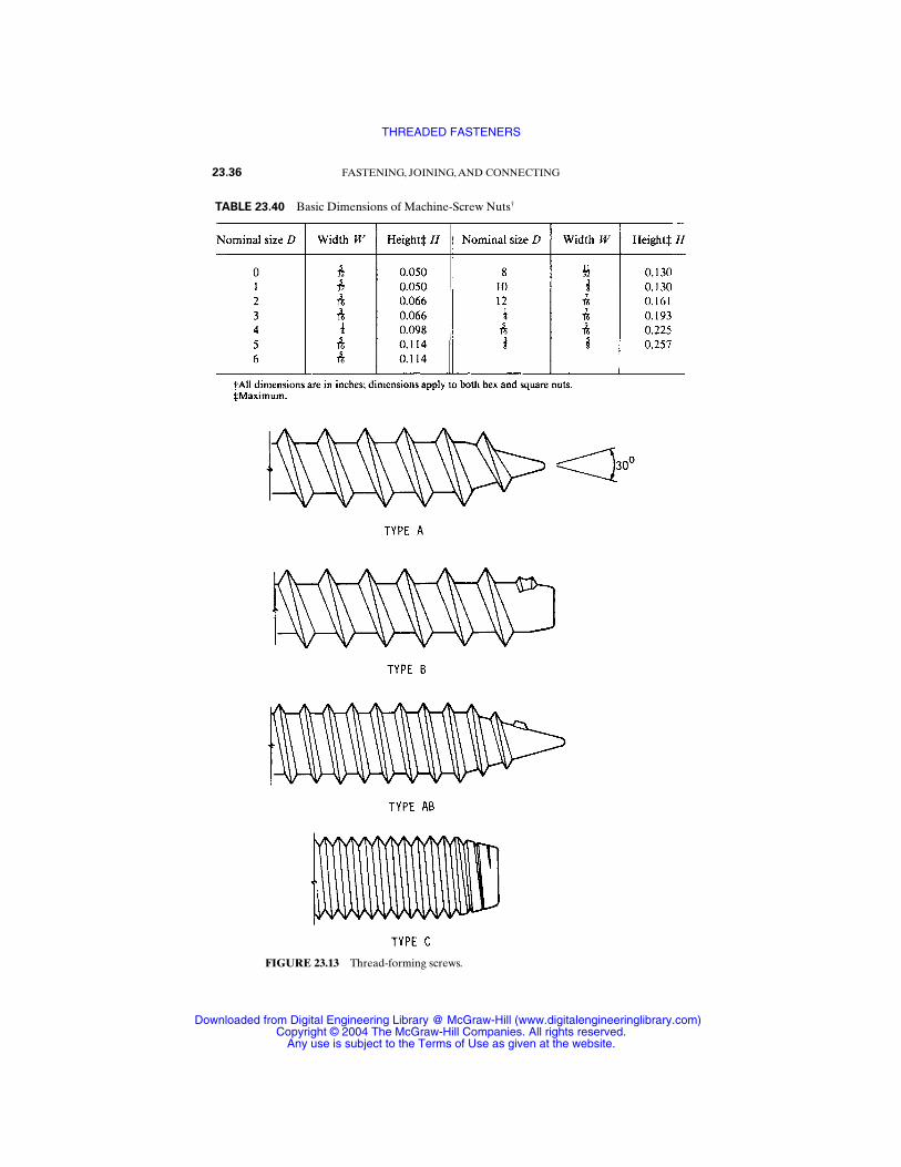
23.36 FASTENING, JOINING, AND CONNECTING
TABLE 23.40 Basic Dimensions of Machine-Screw Nuts†
FIGURE 23.13 Thread-forming screws.
THREADED FASTENERS
Downloaded from Digital Engineering Library @ McGraw-Hill (www.digitalengineeringlibrary.com)Copyright © 2004 The McGraw-Hill Companies. All rights reserved.
Any use is subject to the Terms of Use as given at the website.
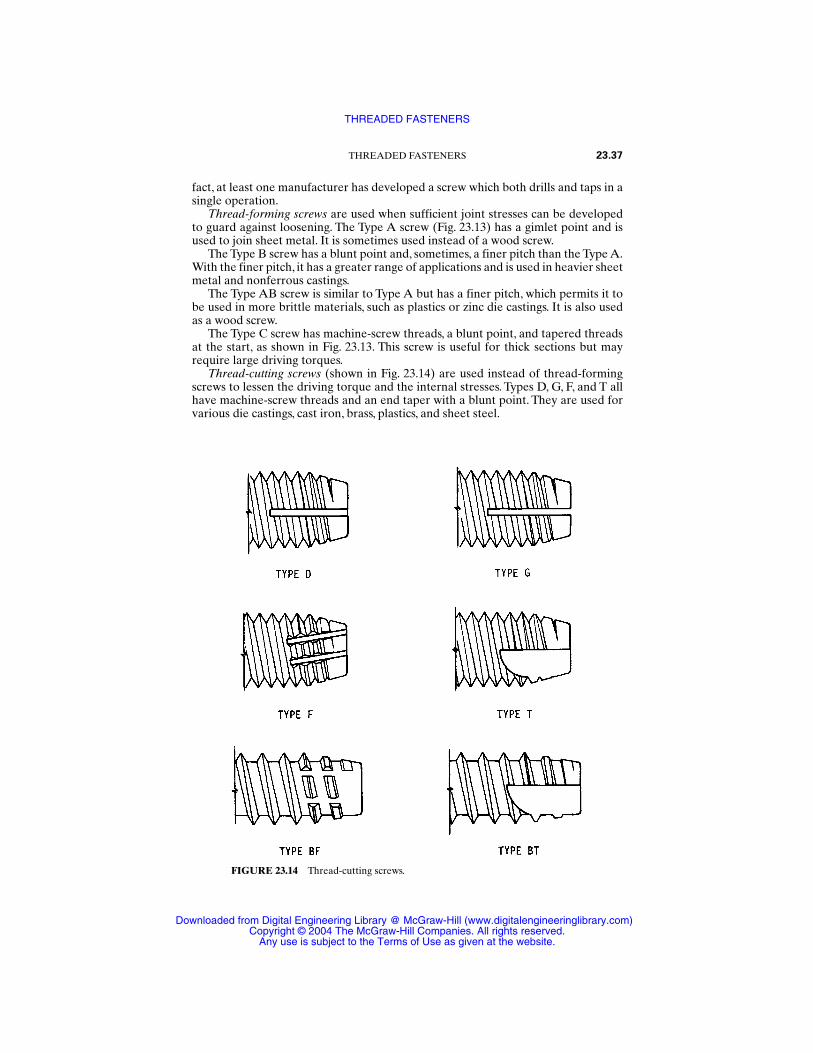
fact, at least one manufacturer has developed a screw which both drills and taps in asingle operation.
Thread-forming screws are used when sufficient joint stresses can be developedto guard against loosening. The Type A screw (Fig. 23.13) has a gimlet point and isused to join sheet metal. It is sometimes used instead of a wood screw.
The Type B screw has a blunt point and, sometimes, a finer pitch than the Type A.With the finer pitch, it has a greater range of applications and is used in heavier sheetmetal and nonferrous castings.
The Type AB screw is similar to Type A but has a finer pitch, which permits it tobe used in more brittle materials, such as plastics or zinc die castings. It is also usedas a wood screw.
The Type C screw has machine-screw threads, a blunt point, and tapered threadsat the start, as shown in Fig. 23.13. This screw is useful for thick sections but mayrequire large driving torques.
Thread-cutting screws (shown in Fig. 23.14) are used instead of thread-formingscrews to lessen the driving torque and the internal stresses. Types D, G, F, and T allhave machine-screw threads and an end taper with a blunt point. They are used forvarious die castings, cast iron, brass, plastics, and sheet steel.
THREADED FASTENERS 23.37
FIGURE 23.14 Thread-cutting screws.
THREADED FASTENERS
Downloaded from Digital Engineering Library @ McGraw-Hill (www.digitalengineeringlibrary.com)Copyright © 2004 The McGraw-Hill Companies. All rights reserved.
Any use is subject to the Terms of Use as given at the website.

Types BF and BT screws (shown in Fig. 23.14) have additional cutting edges anda greater chip-storage capacity. They are useful for various plastics and composi-tions.
Thread-rolling screws (not shown) have a unique point and body shape to makestarting easier and to lessen the driving torque. The thread rolling cold-works thematerial, thus contributing to the strength of the joint.
REFERENCE
23.1 “Codes and Standards; Fasteners,” in ASME Publications Catalog, American Society ofMechanical Engineers, New York, 1985.
23.38 FASTENING, JOINING, AND CONNECTING
THREADED FASTENERS
Downloaded from Digital Engineering Library @ McGraw-Hill (www.digitalengineeringlibrary.com)Copyright © 2004 The McGraw-Hill Companies. All rights reserved.
Any use is subject to the Terms of Use as given at the website.
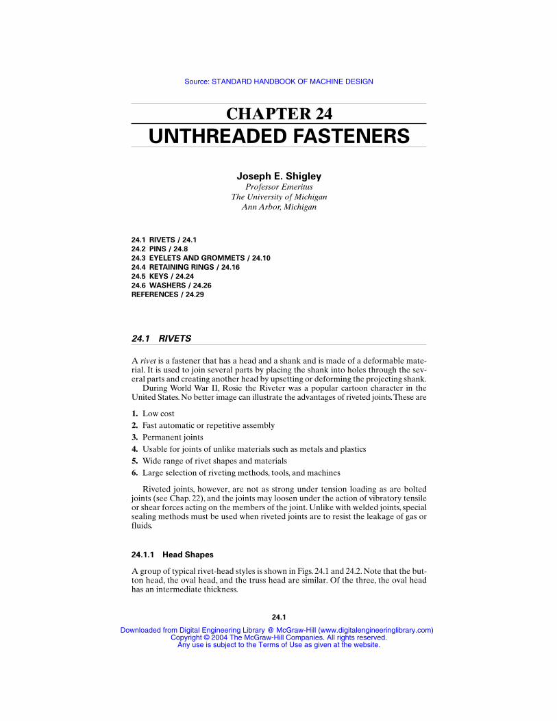
CHAPTER 24UNTHREADED FASTENERS
Joseph E. ShigleyProfessor Emeritus
The University of MichiganAnn Arbor, Michigan
24.1 RIVETS / 24.1
24.2 PINS / 24.8
24.3 EYELETS AND GROMMETS / 24.10
24.4 RETAINING RINGS / 24.16
24.5 KEYS / 24.24
24.6 WASHERS / 24.26
REFERENCES / 24.29
24.1 RIVETS
A rivet is a fastener that has a head and a shank and is made of a deformable mate-rial. It is used to join several parts by placing the shank into holes through the sev-eral parts and creating another head by upsetting or deforming the projecting shank.
During World War II, Rosie the Riveter was a popular cartoon character in theUnited States. No better image can illustrate the advantages of riveted joints.These are
1. Low cost2. Fast automatic or repetitive assembly3. Permanent joints4. Usable for joints of unlike materials such as metals and plastics5. Wide range of rivet shapes and materials6. Large selection of riveting methods, tools, and machines
Riveted joints, however, are not as strong under tension loading as are boltedjoints (see Chap. 22), and the joints may loosen under the action of vibratory tensileor shear forces acting on the members of the joint. Unlike with welded joints, specialsealing methods must be used when riveted joints are to resist the leakage of gas orfluids.
24.1.1 Head Shapes
A group of typical rivet-head styles is shown in Figs. 24.1 and 24.2. Note that the but-ton head, the oval head, and the truss head are similar. Of the three, the oval headhas an intermediate thickness.
24.1
Source: STANDARD HANDBOOK OF MACHINE DESIGN
Downloaded from Digital Engineering Library @ McGraw-Hill (www.digitalengineeringlibrary.com)Copyright © 2004 The McGraw-Hill Companies. All rights reserved.
Any use is subject to the Terms of Use as given at the website.
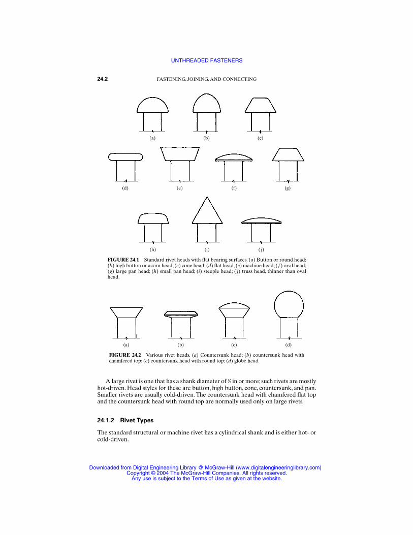
A large rivet is one that has a shank diameter of 1⁄2 in or more; such rivets are mostlyhot-driven. Head styles for these are button, high button, cone, countersunk, and pan.Smaller rivets are usually cold-driven. The countersunk head with chamfered flat topand the countersunk head with round top are normally used only on large rivets.
24.1.2 Rivet Types
The standard structural or machine rivet has a cylindrical shank and is either hot- orcold-driven.
24.2 FASTENING, JOINING, AND CONNECTING
FIGURE 24.1 Standard rivet heads with flat bearing surfaces. (a) Button or round head;(b) high button or acorn head; (c) cone head; (d) flat head; (e) machine head; ( f ) oval head;(g) large pan head; (h) small pan head; (i) steeple head; ( j) truss head, thinner than ovalhead.
FIGURE 24.2 Various rivet heads. (a) Countersunk head; (b) countersunk head withchamfered top; (c) countersunk head with round top; (d) globe head.
(a) (b) (c)
(d) (e) (f) (g)
(h) (i) ( j)
(a) (b) (c) (d)
UNTHREADED FASTENERS
Downloaded from Digital Engineering Library @ McGraw-Hill (www.digitalengineeringlibrary.com)Copyright © 2004 The McGraw-Hill Companies. All rights reserved.
Any use is subject to the Terms of Use as given at the website.
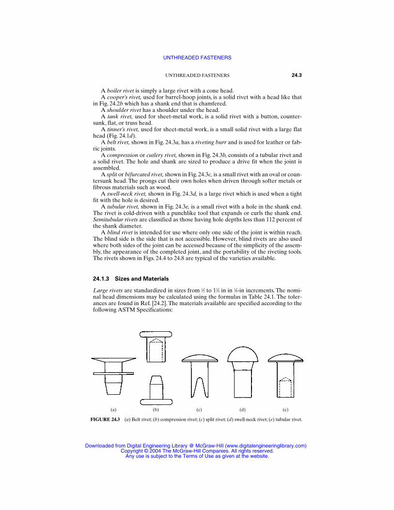
A boiler rivet is simply a large rivet with a cone head.A cooper’s rivet, used for barrel-hoop joints, is a solid rivet with a head like that
in Fig. 24.2b which has a shank end that is chamfered.A shoulder rivet has a shoulder under the head.A tank rivet, used for sheet-metal work, is a solid rivet with a button, counter-
sunk, flat, or truss head.A tinner’s rivet, used for sheet-metal work, is a small solid rivet with a large flat
head (Fig. 24.1d).A belt rivet, shown in Fig. 24.3a, has a riveting burr and is used for leather or fab-
ric joints.A compression or cutlery rivet, shown in Fig. 24.3b, consists of a tubular rivet and
a solid rivet. The hole and shank are sized to produce a drive fit when the joint isassembled.
A split or bifurcated rivet, shown in Fig. 24.3c, is a small rivet with an oval or coun-tersunk head. The prongs cut their own holes when driven through softer metals orfibrous materials such as wood.
A swell-neck rivet, shown in Fig. 24.3d, is a large rivet which is used when a tightfit with the hole is desired.
A tubular rivet, shown in Fig. 24.3e, is a small rivet with a hole in the shank end.The rivet is cold-driven with a punchlike tool that expands or curls the shank end.Semitubular rivets are classified as those having hole depths less than 112 percent ofthe shank diameter.
A blind rivet is intended for use where only one side of the joint is within reach.The blind side is the side that is not accessible. However, blind rivets are also usedwhere both sides of the joint can be accessed because of the simplicity of the assem-bly, the appearance of the completed joint, and the portability of the riveting tools.The rivets shown in Figs. 24.4 to 24.8 are typical of the varieties available.
24.1.3 Sizes and Materials
Large rivets are standardized in sizes from 1⁄2 to 13⁄4 in in 1⁄8-in increments. The nomi-nal head dimensions may be calculated using the formulas in Table 24.1. The toler-ances are found in Ref. [24.2]. The materials available are specified according to thefollowing ASTM Specifications:
UNTHREADED FASTENERS 24.3
FIGURE 24.3 (a) Belt rivet; (b) compression rivet; (c) split rivet; (d) swell-neck rivet; (e) tubular rivet.
(a) (b) (c) (d) (e)
UNTHREADED FASTENERS
Downloaded from Digital Engineering Library @ McGraw-Hill (www.digitalengineeringlibrary.com)Copyright © 2004 The McGraw-Hill Companies. All rights reserved.
Any use is subject to the Terms of Use as given at the website.
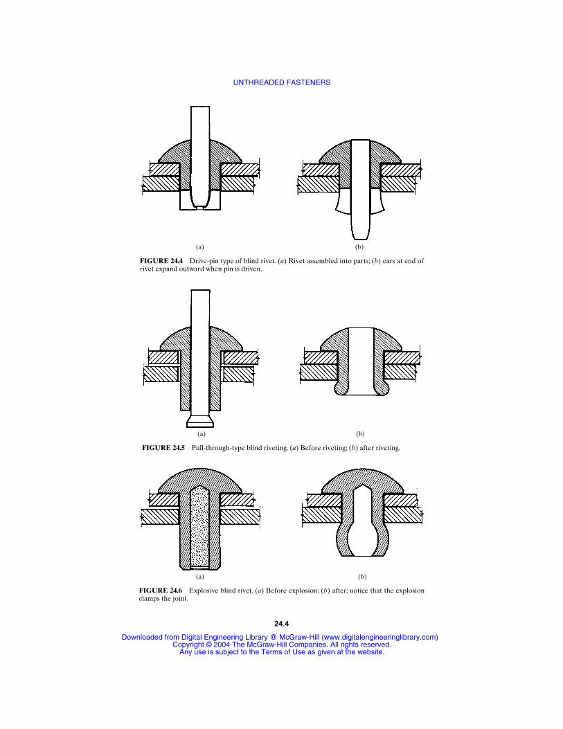
FIGURE 24.4 Drive-pin type of blind rivet. (a) Rivet assembled into parts; (b) ears at end ofrivet expand outward when pin is driven.
(a) (b)
FIGURE 24.5 Pull-through-type blind riveting. (a) Before riveting; (b) after riveting.
(a) (b)
(a)
FIGURE 24.6 Explosive blind rivet. (a) Before explosion; (b) after; notice that the explosionclamps the joint.
(b)
24.4
UNTHREADED FASTENERS
Downloaded from Digital Engineering Library @ McGraw-Hill (www.digitalengineeringlibrary.com)Copyright © 2004 The McGraw-Hill Companies. All rights reserved.
Any use is subject to the Terms of Use as given at the website.
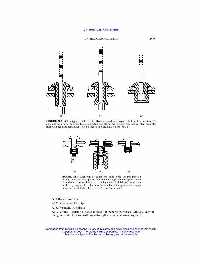
A31 Boiler rivet steel.A131 Rivet steel for ships.A152 Wrought-iron rivets.A502 Grade 1 carbon structural steel for general purposes. Grade 2 carbon-manganese steel for use with high-strength carbon and low-alloy steels.
UNTHREADED FASTENERS 24.5
FIGURE 24.7 Self-plugging blind rivet. (a) Rivet inserted into prepared hole with power tool; (b)axial pull with power tool fills holes completely and clamps work pieces together; (c) stem separatesflush with head and remaining section is locked in place. (Avdel Corporation.)
(a) (b) (c)
FIGURE 24.8 Lock-bolt or collar-type blind rivet. (a) Pin insertedthrough holes and collar placed over the pin tail; (b) nose tool pulls on thepin and reacts against the collar, clamping the work tightly; (c) installationfinished by swaging the collar into the annular locking grooves and sepa-rating the pin at the breaker groove. (Avdel Corporation.)
(a) (b) (c)
UNTHREADED FASTENERS
Downloaded from Digital Engineering Library @ McGraw-Hill (www.digitalengineeringlibrary.com)Copyright © 2004 The McGraw-Hill Companies. All rights reserved.
Any use is subject to the Terms of Use as given at the website.
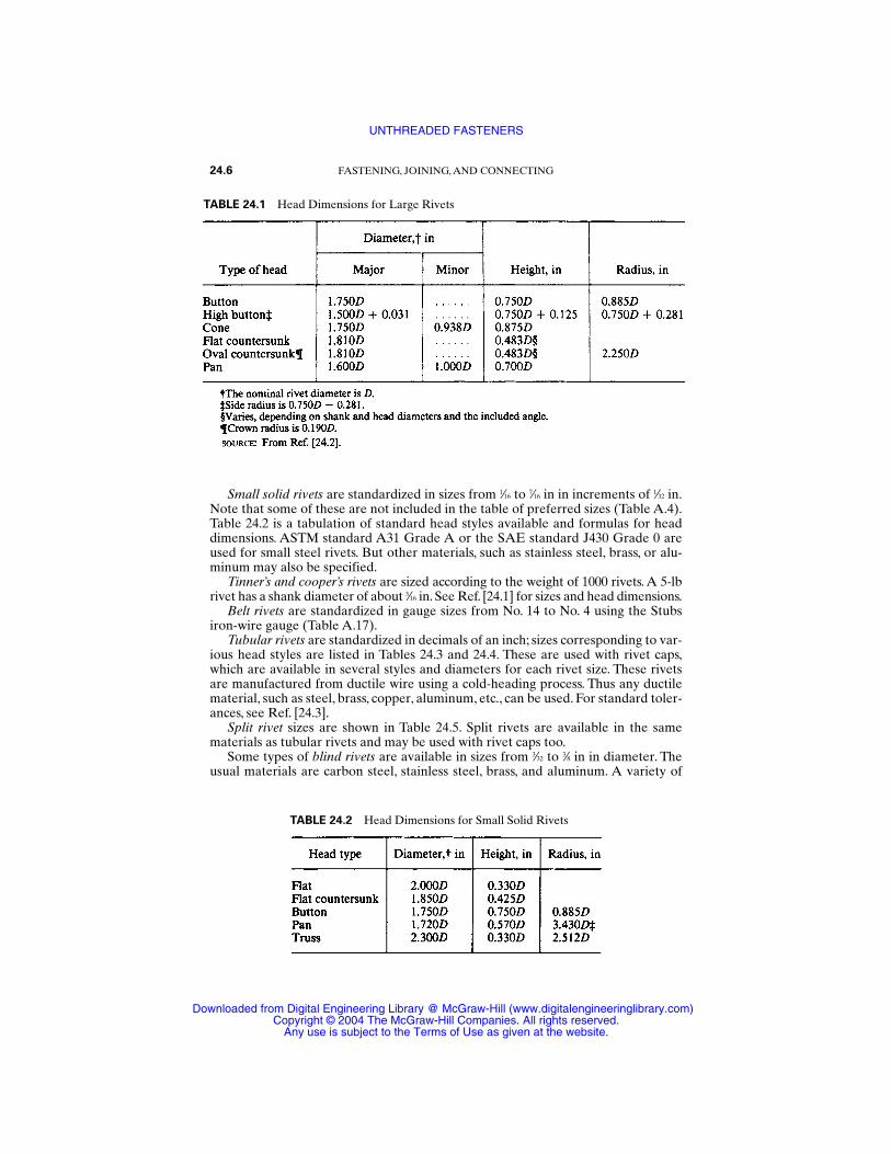
Small solid rivets are standardized in sizes from 1⁄16 to 7⁄16 in in increments of 1⁄32 in.Note that some of these are not included in the table of preferred sizes (Table A.4).Table 24.2 is a tabulation of standard head styles available and formulas for headdimensions. ASTM standard A31 Grade A or the SAE standard J430 Grade 0 areused for small steel rivets. But other materials, such as stainless steel, brass, or alu-minum may also be specified.
Tinner’s and cooper’s rivets are sized according to the weight of 1000 rivets. A 5-lbrivet has a shank diameter of about 3⁄16 in. See Ref. [24.1] for sizes and head dimensions.
Belt rivets are standardized in gauge sizes from No. 14 to No. 4 using the Stubsiron-wire gauge (Table A.17).
Tubular rivets are standardized in decimals of an inch; sizes corresponding to var-ious head styles are listed in Tables 24.3 and 24.4. These are used with rivet caps,which are available in several styles and diameters for each rivet size. These rivetsare manufactured from ductile wire using a cold-heading process. Thus any ductilematerial, such as steel, brass, copper, aluminum, etc., can be used. For standard toler-ances, see Ref. [24.3].
Split rivet sizes are shown in Table 24.5. Split rivets are available in the samematerials as tubular rivets and may be used with rivet caps too.
Some types of blind rivets are available in sizes from 3⁄32 to 3⁄8 in in diameter. Theusual materials are carbon steel, stainless steel, brass, and aluminum. A variety of
24.6 FASTENING, JOINING, AND CONNECTING
TABLE 24.1 Head Dimensions for Large Rivets
TABLE 24.2 Head Dimensions for Small Solid Rivets
UNTHREADED FASTENERS
Downloaded from Digital Engineering Library @ McGraw-Hill (www.digitalengineeringlibrary.com)Copyright © 2004 The McGraw-Hill Companies. All rights reserved.
Any use is subject to the Terms of Use as given at the website.
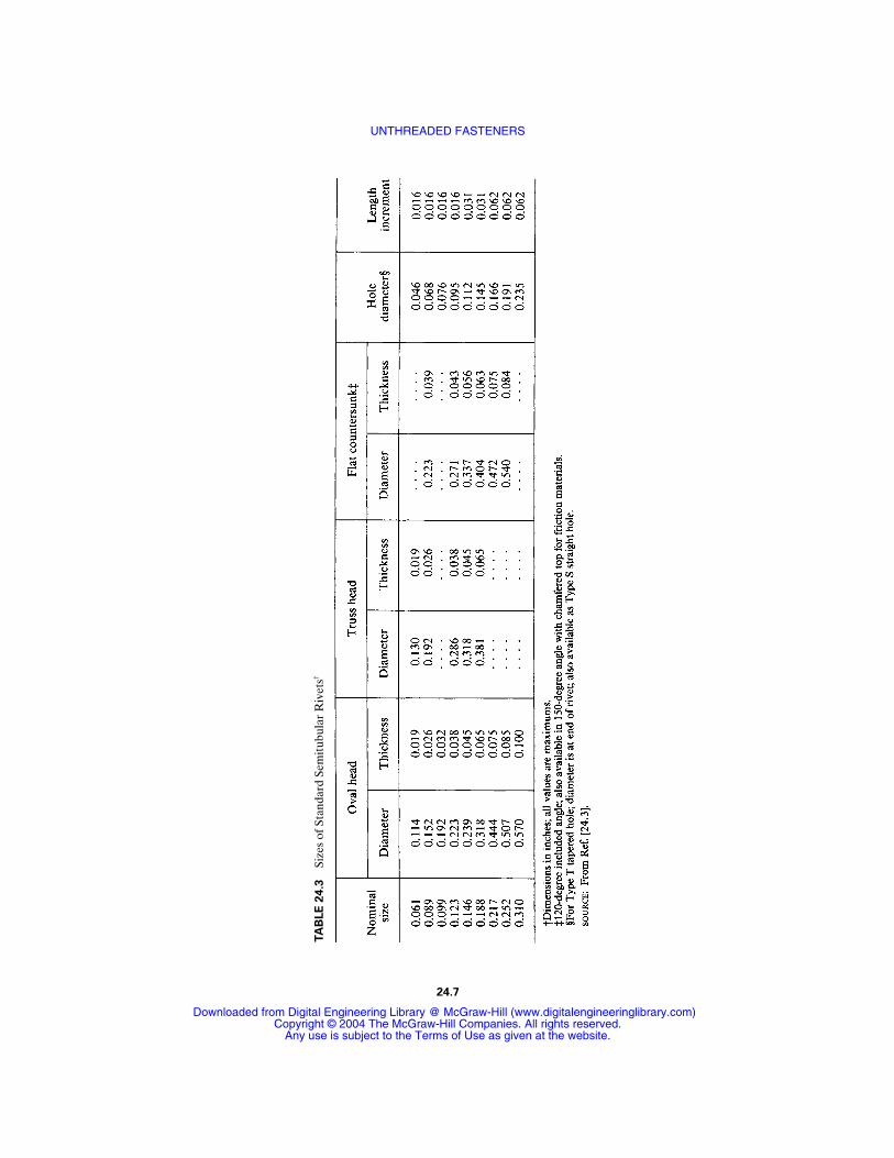
TA
BLE
24.3
Size
s of
Sta
ndar
d Se
mit
ubul
ar R
ivet
s†
24.7
UNTHREADED FASTENERS
Downloaded from Digital Engineering Library @ McGraw-Hill (www.digitalengineeringlibrary.com)Copyright © 2004 The McGraw-Hill Companies. All rights reserved.
Any use is subject to the Terms of Use as given at the website.
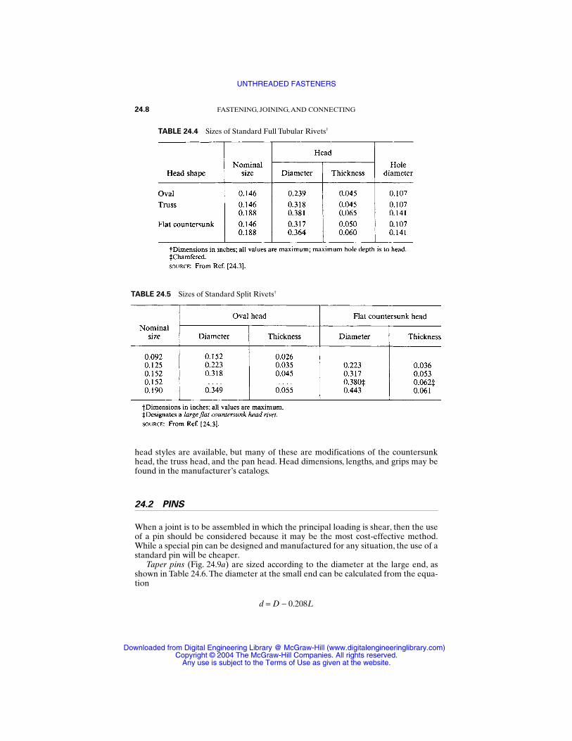
head styles are available, but many of these are modifications of the countersunkhead, the truss head, and the pan head. Head dimensions, lengths, and grips may befound in the manufacturer’s catalogs.
24.2 PINS
When a joint is to be assembled in which the principal loading is shear, then the useof a pin should be considered because it may be the most cost-effective method.While a special pin can be designed and manufactured for any situation, the use of astandard pin will be cheaper.
Taper pins (Fig. 24.9a) are sized according to the diameter at the large end, asshown in Table 24.6. The diameter at the small end can be calculated from the equa-tion
d = D − 0.208L
24.8 FASTENING, JOINING, AND CONNECTING
TABLE 24.4 Sizes of Standard Full Tubular Rivets†
TABLE 24.5 Sizes of Standard Split Rivets†
UNTHREADED FASTENERS
Downloaded from Digital Engineering Library @ McGraw-Hill (www.digitalengineeringlibrary.com)Copyright © 2004 The McGraw-Hill Companies. All rights reserved.
Any use is subject to the Terms of Use as given at the website.
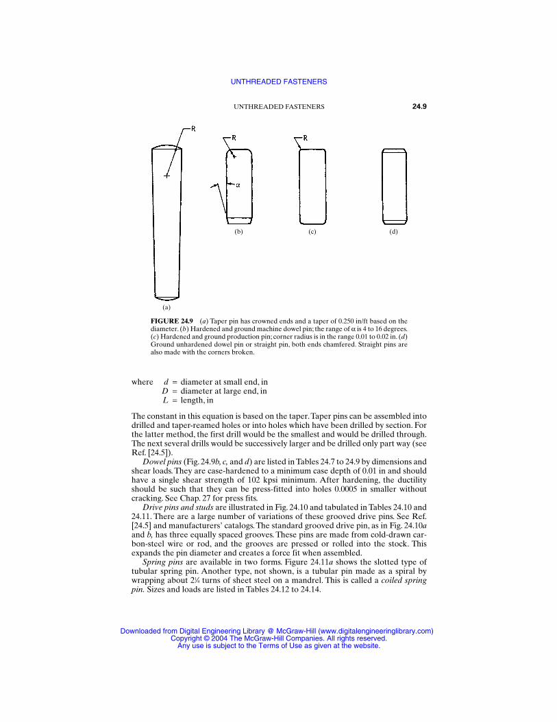
where d = diameter at small end, inD = diameter at large end, inL = length, in
The constant in this equation is based on the taper.Taper pins can be assembled intodrilled and taper-reamed holes or into holes which have been drilled by section. Forthe latter method, the first drill would be the smallest and would be drilled through.The next several drills would be successively larger and be drilled only part way (seeRef. [24.5]).
Dowel pins (Fig. 24.9b, c, and d) are listed in Tables 24.7 to 24.9 by dimensions andshear loads. They are case-hardened to a minimum case depth of 0.01 in and shouldhave a single shear strength of 102 kpsi minimum. After hardening, the ductilityshould be such that they can be press-fitted into holes 0.0005 in smaller withoutcracking. See Chap. 27 for press fits.
Drive pins and studs are illustrated in Fig. 24.10 and tabulated in Tables 24.10 and24.11. There are a large number of variations of these grooved drive pins. See Ref.[24.5] and manufacturers’ catalogs. The standard grooved drive pin, as in Fig. 24.10aand b, has three equally spaced grooves. These pins are made from cold-drawn car-bon-steel wire or rod, and the grooves are pressed or rolled into the stock. Thisexpands the pin diameter and creates a force fit when assembled.
Spring pins are available in two forms. Figure 24.11a shows the slotted type oftubular spring pin. Another type, not shown, is a tubular pin made as a spiral bywrapping about 21⁄4 turns of sheet steel on a mandrel. This is called a coiled springpin. Sizes and loads are listed in Tables 24.12 to 24.14.
UNTHREADED FASTENERS 24.9
FIGURE 24.9 (a) Taper pin has crowned ends and a taper of 0.250 in/ft based on thediameter. (b) Hardened and ground machine dowel pin; the range of α is 4 to 16 degrees.(c) Hardened and ground production pin; corner radius is in the range 0.01 to 0.02 in. (d)Ground unhardened dowel pin or straight pin, both ends chamfered. Straight pins arealso made with the corners broken.
(a)
(b) (c) (d)
UNTHREADED FASTENERS
Downloaded from Digital Engineering Library @ McGraw-Hill (www.digitalengineeringlibrary.com)Copyright © 2004 The McGraw-Hill Companies. All rights reserved.
Any use is subject to the Terms of Use as given at the website.
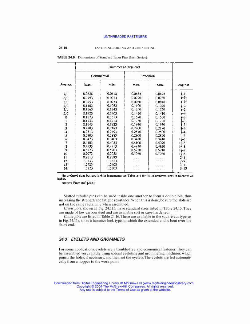
Slotted tubular pins can be used inside one another to form a double pin, thusincreasing the strength and fatigue resistance.When this is done, be sure the slots arenot on the same radial line when assembled.
Clevis pins, shown in Fig. 24.11b, have standard sizes listed in Table 24.15. Theyare made of low-carbon steel and are available soft or case-hardened.
Cotter pins are listed in Table 24.16. These are available in the square-cut type, asin Fig. 24.11c, or as a hammer-lock type, in which the extended end is bent over theshort end.
24.3 EYELETS AND GROMMETS
For some applications, eyelets are a trouble-free and economical fastener. They canbe assembled very rapidly using special eyeleting and grommeting machines, whichpunch the holes, if necessary, and then set the eyelets. The eyelets are fed automati-cally from a hopper to the work point.
24.10 FASTENING, JOINING, AND CONNECTING
TABLE 24.6 Dimensions of Standard Taper Pins (Inch Series)
UNTHREADED FASTENERS
Downloaded from Digital Engineering Library @ McGraw-Hill (www.digitalengineeringlibrary.com)Copyright © 2004 The McGraw-Hill Companies. All rights reserved.
Any use is subject to the Terms of Use as given at the website.

UNTHREADED FASTENERS 24.11
TABLE 24.7 Dimensions of Hardened Ground Machine Dowel Pins (Inch Series) (Fig. 24.9b)
TABLE 24.8 Dimensions of Hardened Ground Production Dowel Pins (Inch Series) (Fig. 24.9c)
UNTHREADED FASTENERS
Downloaded from Digital Engineering Library @ McGraw-Hill (www.digitalengineeringlibrary.com)Copyright © 2004 The McGraw-Hill Companies. All rights reserved.
Any use is subject to the Terms of Use as given at the website.
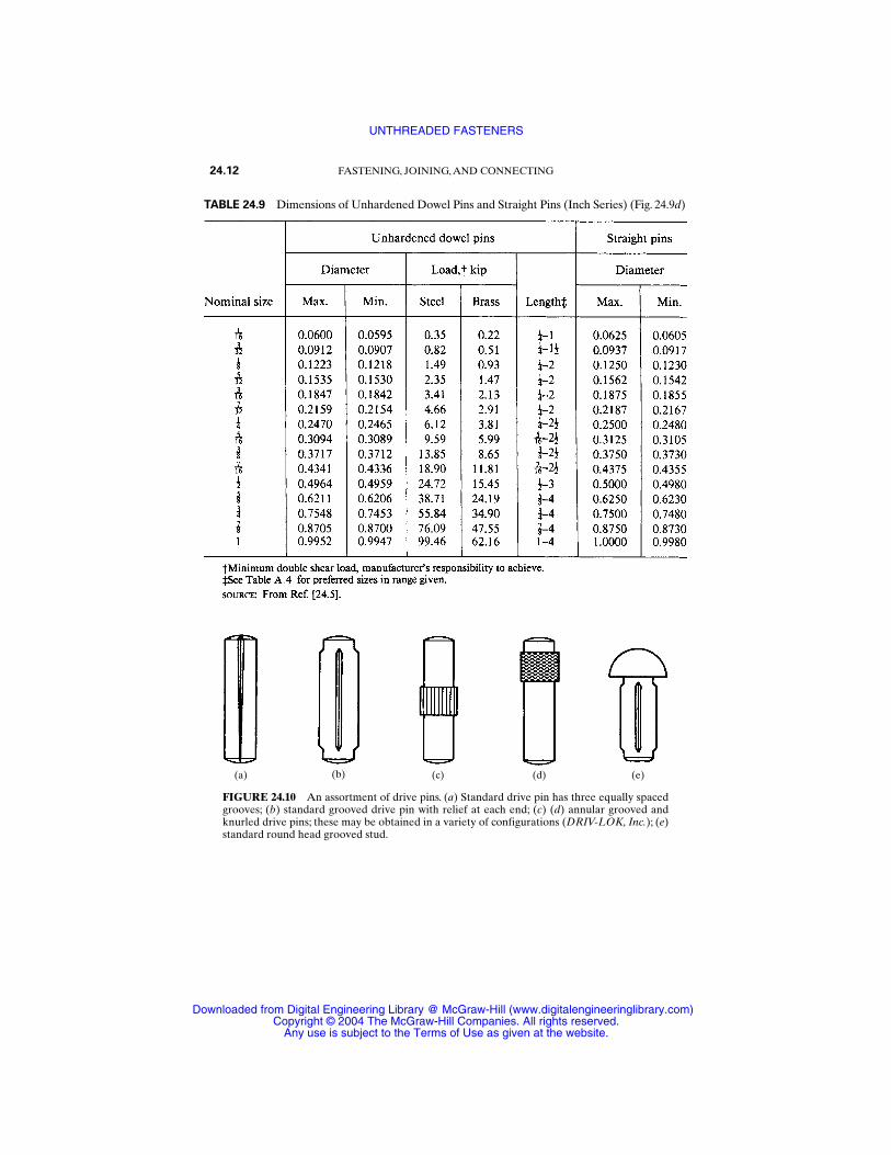
24.12 FASTENING, JOINING, AND CONNECTING
TABLE 24.9 Dimensions of Unhardened Dowel Pins and Straight Pins (Inch Series) (Fig. 24.9d)
FIGURE 24.10 An assortment of drive pins. (a) Standard drive pin has three equally spacedgrooves; (b) standard grooved drive pin with relief at each end; (c) (d) annular grooved andknurled drive pins; these may be obtained in a variety of configurations (DRIV-LOK, Inc.); (e)standard round head grooved stud.
(a) (b) (c) (d) (e)
UNTHREADED FASTENERS
Downloaded from Digital Engineering Library @ McGraw-Hill (www.digitalengineeringlibrary.com)Copyright © 2004 The McGraw-Hill Companies. All rights reserved.
Any use is subject to the Terms of Use as given at the website.
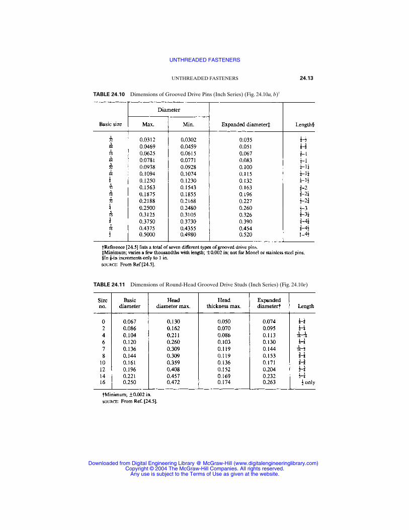
UNTHREADED FASTENERS 24.13
TABLE 24.10 Dimensions of Grooved Drive Pins (Inch Series) (Fig. 24.10a, b)†
TABLE 24.11 Dimensions of Round-Head Grooved Drive Studs (Inch Series) (Fig. 24.10e)
UNTHREADED FASTENERS
Downloaded from Digital Engineering Library @ McGraw-Hill (www.digitalengineeringlibrary.com)Copyright © 2004 The McGraw-Hill Companies. All rights reserved.
Any use is subject to the Terms of Use as given at the website.
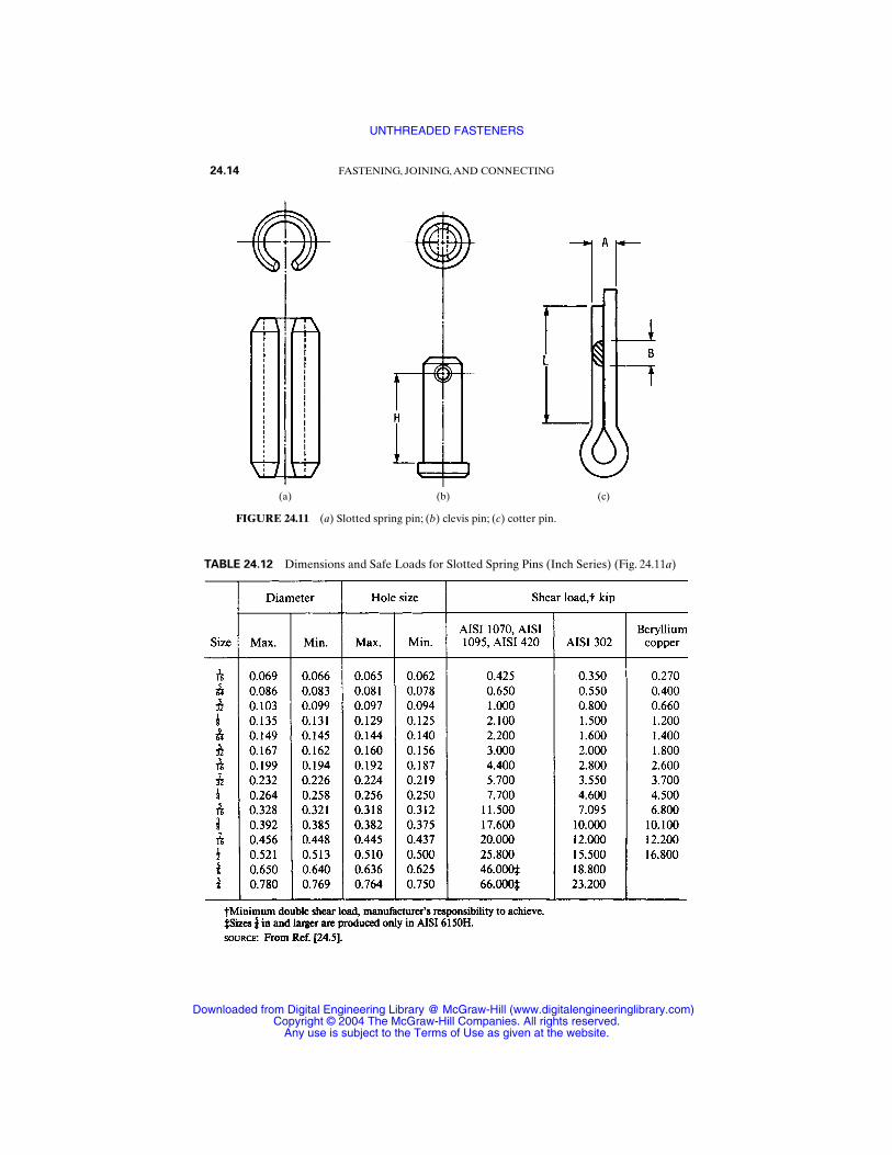
24.14 FASTENING, JOINING, AND CONNECTING
FIGURE 24.11 (a) Slotted spring pin; (b) clevis pin; (c) cotter pin.
(a) (b) (c)
TABLE 24.12 Dimensions and Safe Loads for Slotted Spring Pins (Inch Series) (Fig. 24.11a)
UNTHREADED FASTENERS
Downloaded from Digital Engineering Library @ McGraw-Hill (www.digitalengineeringlibrary.com)Copyright © 2004 The McGraw-Hill Companies. All rights reserved.
Any use is subject to the Terms of Use as given at the website.
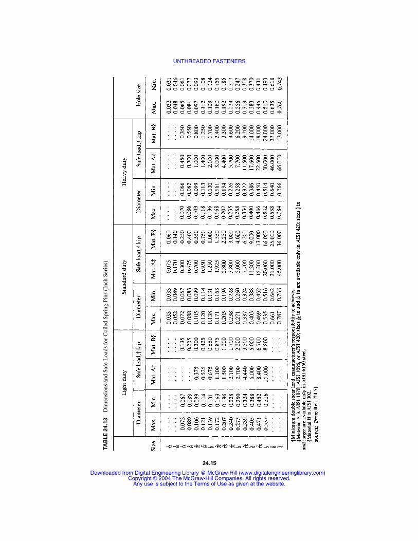
TA
BLE
24.1
3D
imen
sion
s an
d Sa
fe L
oads
for
Coi
led
Spri
ng P
ins
(Inc
h Se
ries
)
24.15
UNTHREADED FASTENERS
Downloaded from Digital Engineering Library @ McGraw-Hill (www.digitalengineeringlibrary.com)Copyright © 2004 The McGraw-Hill Companies. All rights reserved.
Any use is subject to the Terms of Use as given at the website.
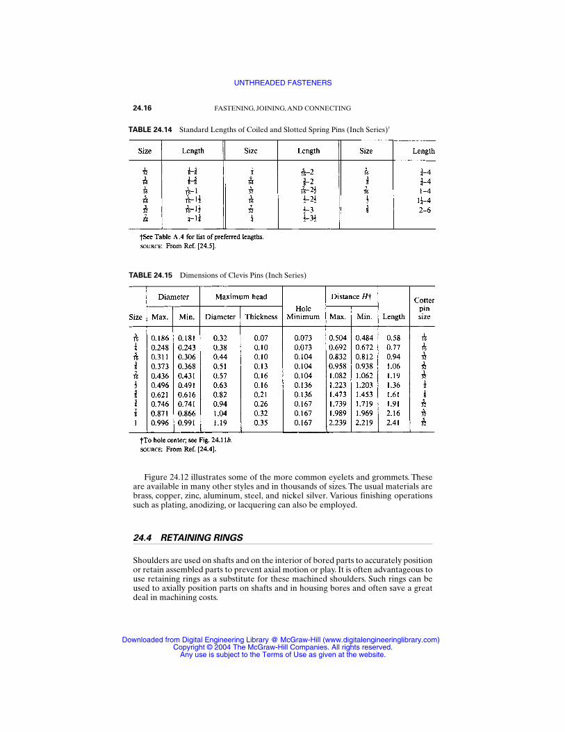
Figure 24.12 illustrates some of the more common eyelets and grommets. Theseare available in many other styles and in thousands of sizes. The usual materials arebrass, copper, zinc, aluminum, steel, and nickel silver. Various finishing operationssuch as plating, anodizing, or lacquering can also be employed.
24.4 RETAINING RINGS
Shoulders are used on shafts and on the interior of bored parts to accurately positionor retain assembled parts to prevent axial motion or play. It is often advantageous touse retaining rings as a substitute for these machined shoulders. Such rings can beused to axially position parts on shafts and in housing bores and often save a greatdeal in machining costs.
24.16 FASTENING, JOINING, AND CONNECTING
TABLE 24.14 Standard Lengths of Coiled and Slotted Spring Pins (Inch Series)†
TABLE 24.15 Dimensions of Clevis Pins (Inch Series)
UNTHREADED FASTENERS
Downloaded from Digital Engineering Library @ McGraw-Hill (www.digitalengineeringlibrary.com)Copyright © 2004 The McGraw-Hill Companies. All rights reserved.
Any use is subject to the Terms of Use as given at the website.

UNTHREADED FASTENERS 24.17
TABLE 24.16 Dimensions of Cotter Pins (Inch Series) (Fig. 24.11c)
FIGURE 24.12 (a) Flat-flange eyelet; (b) funnel-flange eyelet; (c) rolled-flange eyelet;(d) telescoping eyelet with neck washer; (e) plain grommet; (f ) toothed grommet.
(a) (b) (c)
(d) (e) (f)
UNTHREADED FASTENERS
Downloaded from Digital Engineering Library @ McGraw-Hill (www.digitalengineeringlibrary.com)Copyright © 2004 The McGraw-Hill Companies. All rights reserved.
Any use is subject to the Terms of Use as given at the website.
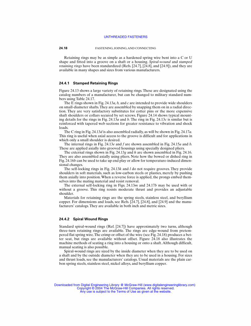
Retaining rings may be as simple as a hardened spring wire bent into a C or Ushape and fitted into a groove on a shaft or a housing. Spiral-wound and stampedretaining rings have been standardized (Refs. [24.7], [24.8], and [24.9]), and they areavailable in many shapes and sizes from various manufacturers.
24.4.1 Stamped Retaining Rings
Figure 24.13 shows a large variety of retaining rings. These are designated using thecatalog numbers of a manufacturer, but can be changed to military standard num-bers using Table 24.17.
The E rings shown in Fig. 24.13a, b, and c are intended to provide wide shoulderson small-diameter shafts.They are assembled by snapping them on in a radial direc-tion. They are very satisfactory substitutes for cotter pins or the more expensiveshaft shoulders or collars secured by set screws. Figure 24.14 shows typical mount-ing details for the rings in Fig. 24.13a and b. The ring in Fig. 24.13c is similar but isreinforced with tapered web sections for greater resistance to vibration and shockloads.
The C ring in Fig. 24.13d is also assembled radially, as will be shown in Fig. 24.17a.This ring is useful when axial access to the groove is difficult and for applications inwhich only a small shoulder is desired.
The internal rings in Fig. 24.13e and f are shown assembled in Fig. 24.15a and b.These are applied axially into grooved housings using specially designed pliers.
The external rings shown in Fig. 24.13g and h are shown assembled in Fig. 24.16.They are also assembled axially using pliers. Note how the bowed or dished ring inFig. 24.16b can be used to take up end play or allow for temperature-induced dimen-sional changes.
The self-locking rings in Fig. 24.13k and l do not require grooves. They provideshoulders in soft materials, such as low-carbon steels or plastics, merely by pushingthem axially into position. When a reverse force is applied, the prongs embed them-selves into the mating material and resist removal.
The external self-locking ring in Figs. 24.13m and 24.17b may be used with orwithout a groove. This ring resists moderate thrust and provides an adjustableshoulder.
Materials for retaining rings are the spring steels, stainless steel, and berylliumcopper. For dimensions and loads, see Refs. [24.7], [24.8], and [24.9] and the manu-facturers’ catalogs. They are available in both inch and metric sizes.
24.4.2 Spiral Wound Rings
Standard spiral-wound rings (Ref. [24.7]) have approximately two turns, althoughthree-turn retaining rings are available. The rings are edge-wound from pretem-pered flat spring wire.The crimp or offset of the wire (see Fig. 24.18) produces a bet-ter seat, but rings are available without offset. Figure 24.18 also illustrates themachine methods of seating a ring into a housing or onto a shaft. Although difficult,manual seating is also possible.
Spiral-wound rings are sized by the inside diameter when they are to be used ona shaft and by the outside diameter when they are to be used in a housing. For sizesand thrust loads, see the manufacturers’ catalogs. Usual materials are the plain car-bon spring steels, stainless steel, nickel alloys, and beryllium copper.
24.18 FASTENING, JOINING, AND CONNECTING
UNTHREADED FASTENERS
Downloaded from Digital Engineering Library @ McGraw-Hill (www.digitalengineeringlibrary.com)Copyright © 2004 The McGraw-Hill Companies. All rights reserved.
Any use is subject to the Terms of Use as given at the website.
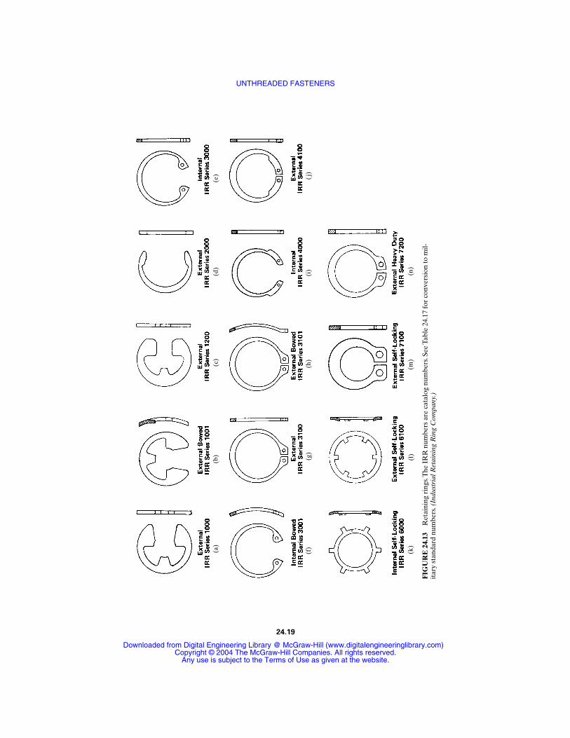
FIG
UR
E 2
4.13
Ret
aini
ng r
ings
.The
IR
R n
umbe
rs a
re c
atal
og n
umbe
rs.S
ee T
able
24.
17 fo
r co
nver
sion
to m
il-it
ary
stan
dard
num
bers
.(In
dust
rial
Ret
aini
ng R
ing
Com
pany
.)
(a)
(b)
(c)
(d)
(e)
(f)
(g)
(h)
(i)
(j)
(k)
(l)
(m)
(n)
24.19
UNTHREADED FASTENERS
Downloaded from Digital Engineering Library @ McGraw-Hill (www.digitalengineeringlibrary.com)Copyright © 2004 The McGraw-Hill Companies. All rights reserved.
Any use is subject to the Terms of Use as given at the website.
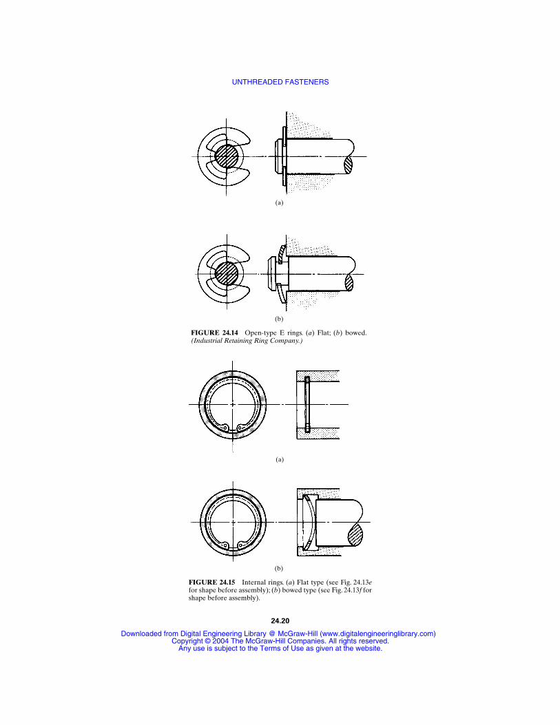
FIGURE 24.14 Open-type E rings. (a) Flat; (b) bowed.(Industrial Retaining Ring Company.)
(a)
(b)
FIGURE 24.15 Internal rings. (a) Flat type (see Fig. 24.13efor shape before assembly); (b) bowed type (see Fig. 24.13f forshape before assembly).
(a)
(b)
24.20
UNTHREADED FASTENERS
Downloaded from Digital Engineering Library @ McGraw-Hill (www.digitalengineeringlibrary.com)Copyright © 2004 The McGraw-Hill Companies. All rights reserved.
Any use is subject to the Terms of Use as given at the website.
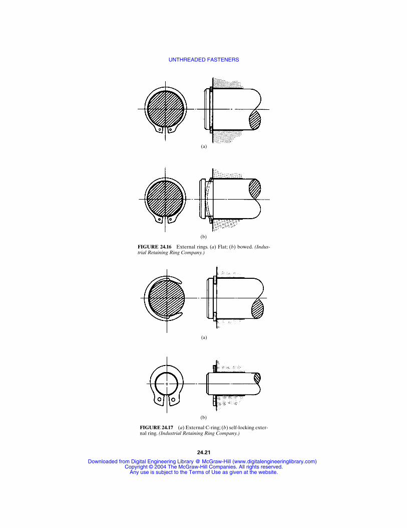
FIGURE 24.16 External rings. (a) Flat; (b) bowed. (Indus-trial Retaining Ring Company.)
(a)
(b)
FIGURE 24.17 (a) External C-ring; (b) self-locking exter-nal ring. (Industrial Retaining Ring Company.)
(a)
(b)
24.21
UNTHREADED FASTENERS
Downloaded from Digital Engineering Library @ McGraw-Hill (www.digitalengineeringlibrary.com)Copyright © 2004 The McGraw-Hill Companies. All rights reserved.
Any use is subject to the Terms of Use as given at the website.
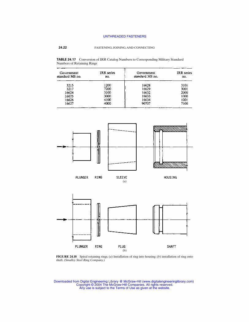
24.22 FASTENING, JOINING, AND CONNECTING
FIGURE 24.18 Spiral retaining rings. (a) Installation of ring into housing; (b) installation of ring ontoshaft. (Smalley Steel Ring Company.)
(a)
(b)
TABLE 24.17 Conversion of IRR Catalog Numbers to Corresponding Military StandardNumbers of Retaining Rings
UNTHREADED FASTENERS
Downloaded from Digital Engineering Library @ McGraw-Hill (www.digitalengineeringlibrary.com)Copyright © 2004 The McGraw-Hill Companies. All rights reserved.
Any use is subject to the Terms of Use as given at the website.

UNTHREADED FASTENERS 24.23
FIGURE 24.19 (a) Square or rectangular key. (b) Square or rectangular key with one end rounded;also available with both ends rounded. (c) Square or rectangular key with gib head. (d) Woodruff key;also available with flattened bottom. (e) Tapered rectangular key; = hub length, h = height; taper is 1⁄8in for 12 in or 1 for 100 for metric sizes. (f ) Tapered gib-head key; dimensions and taper same as in (e).
(a) (b)
(c)
(d)
(e) (f)
UNTHREADED FASTENERS
Downloaded from Digital Engineering Library @ McGraw-Hill (www.digitalengineeringlibrary.com)Copyright © 2004 The McGraw-Hill Companies. All rights reserved.
Any use is subject to the Terms of Use as given at the website.
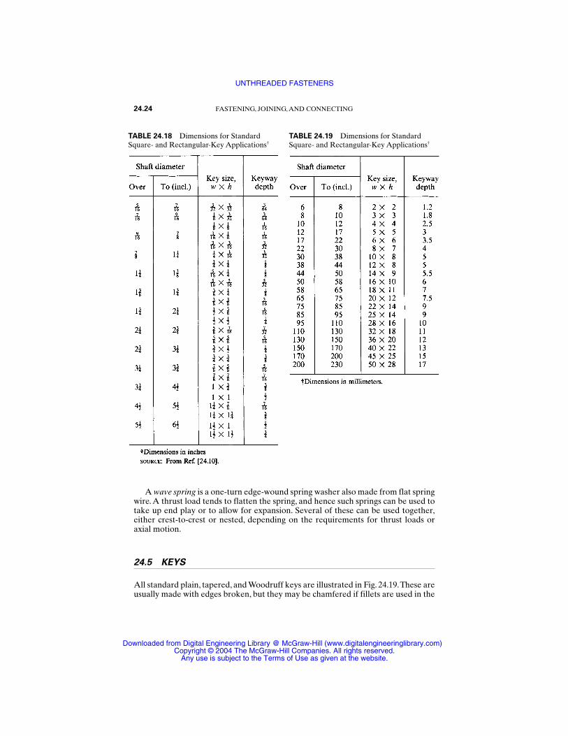
A wave spring is a one-turn edge-wound spring washer also made from flat springwire. A thrust load tends to flatten the spring, and hence such springs can be used totake up end play or to allow for expansion. Several of these can be used together,either crest-to-crest or nested, depending on the requirements for thrust loads oraxial motion.
24.5 KEYS
All standard plain, tapered, and Woodruff keys are illustrated in Fig. 24.19.These areusually made with edges broken, but they may be chamfered if fillets are used in the
24.24 FASTENING, JOINING, AND CONNECTING
TABLE 24.18 Dimensions for StandardSquare- and Rectangular-Key Applications†
TABLE 24.19 Dimensions for StandardSquare- and Rectangular-Key Applications†
UNTHREADED FASTENERS
Downloaded from Digital Engineering Library @ McGraw-Hill (www.digitalengineeringlibrary.com)Copyright © 2004 The McGraw-Hill Companies. All rights reserved.
Any use is subject to the Terms of Use as given at the website.
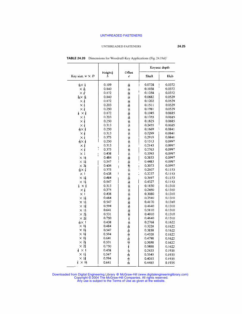
UNTHREADED FASTENERS 24.25
TABLE 24.20 Dimensions for Woodruff-Key Applications (Fig. 24.19d)†
UNTHREADED FASTENERS
Downloaded from Digital Engineering Library @ McGraw-Hill (www.digitalengineeringlibrary.com)Copyright © 2004 The McGraw-Hill Companies. All rights reserved.
Any use is subject to the Terms of Use as given at the website.
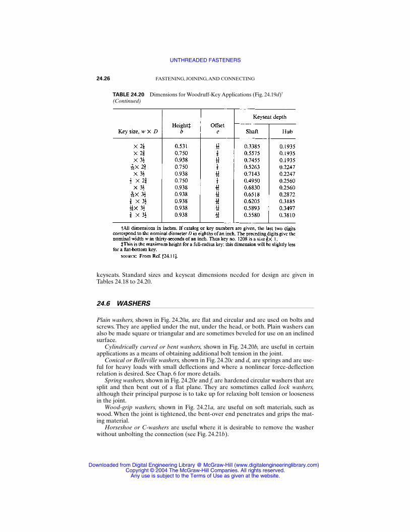
keyseats. Standard sizes and keyseat dimensions needed for design are given inTables 24.18 to 24.20.
24.6 WASHERS
Plain washers, shown in Fig. 24.20a, are flat and circular and are used on bolts andscrews. They are applied under the nut, under the head, or both. Plain washers canalso be made square or triangular and are sometimes beveled for use on an inclinedsurface.
Cylindrically curved or bent washers, shown in Fig. 24.20b, are useful in certainapplications as a means of obtaining additional bolt tension in the joint.
Conical or Belleville washers, shown in Fig. 24.20c and d, are springs and are use-ful for heavy loads with small deflections and where a nonlinear force-deflectionrelation is desired. See Chap. 6 for more details.
Spring washers, shown in Fig. 24.20e and f, are hardened circular washers that aresplit and then bent out of a flat plane. They are sometimes called lock washers,although their principal purpose is to take up for relaxing bolt tension or loosenessin the joint.
Wood-grip washers, shown in Fig. 24.21a, are useful on soft materials, such aswood. When the joint is tightened, the bent-over end penetrates and grips the mat-ing material.
Horseshoe or C-washers are useful where it is desirable to remove the washerwithout unbolting the connection (see Fig. 24.21b).
24.26 FASTENING, JOINING, AND CONNECTING
TABLE 24.20 Dimensions for Woodruff-Key Applications (Fig. 24.19d)†
(Continued)
UNTHREADED FASTENERS
Downloaded from Digital Engineering Library @ McGraw-Hill (www.digitalengineeringlibrary.com)Copyright © 2004 The McGraw-Hill Companies. All rights reserved.
Any use is subject to the Terms of Use as given at the website.
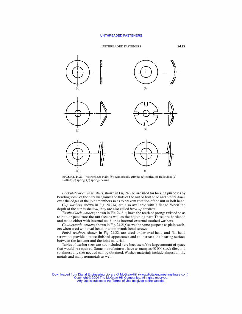
Lockplate or eared washers, shown in Fig. 24.21c, are used for locking purposes bybending some of the ears up against the flats of the nut or bolt head and others downover the edges of the joint members so as to prevent rotation of the nut or bolt head.
Cup washers, shown in Fig. 24.21d, are also available with a flange. When thedepth of the cup is shallow, they are also called back-up washers.
Toothed lock washers, shown in Fig. 24.21e, have the teeth or prongs twisted so asto bite or penetrate the nut face as well as the adjoining part. These are hardenedand made either with internal teeth or as internal-external toothed washers.
Countersunk washers, shown in Fig. 24.21f, serve the same purpose as plain wash-ers when used with oval-head or countersunk-head screws.
Finish washers, shown in Fig. 24.22, are used under oval-head and flat-headscrews to provide a more finished appearance and to increase the bearing surfacebetween the fastener and the joint material.
Tables of washer sizes are not included here because of the large amount of spacethat would be required. Some manufacturers have as many as 60 000 stock dies, andso almost any size needed can be obtained. Washer materials include almost all themetals and many nonmetals as well.
UNTHREADED FASTENERS 24.27
FIGURE 24.20 Washers. (a) Plain; (b) cylindrically curved; (c) conical or Belleville; (d)slotted; (e) spring; (f ) spring-locking.
(a) (b)
(c) (d)
(e) (f)
UNTHREADED FASTENERS
Downloaded from Digital Engineering Library @ McGraw-Hill (www.digitalengineeringlibrary.com)Copyright © 2004 The McGraw-Hill Companies. All rights reserved.
Any use is subject to the Terms of Use as given at the website.
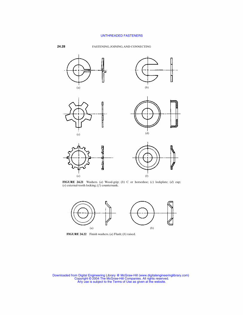
24.28 FASTENING, JOINING, AND CONNECTING
FIGURE 24.22 Finish washers. (a) Flush; (b) raised.
(a) (b)
FIGURE 24.21 Washers. (a) Wood-grip; (b) C or horseshoe; (c) lockplate; (d) cup;(e) external-tooth locking; (f ) countersunk.
(a) (b)
(c) (d)
(e) (f)
UNTHREADED FASTENERS
Downloaded from Digital Engineering Library @ McGraw-Hill (www.digitalengineeringlibrary.com)Copyright © 2004 The McGraw-Hill Companies. All rights reserved.
Any use is subject to the Terms of Use as given at the website.

REFERENCES†
24.1 ANSI B18.1.1-1972 (R2001), “Small Solid Rivets.”
24.2 ANSI B18.1.2-1972 (R2001), “Large Rivets.”
24.3 ANSI B18.7-1972 (R2001), “General Purpose Semi-Tubular Rivets, Full Tubular Rivets,Split Rivets, and Rivet Caps.”
24.4 ANSI B18.8.1-1994, “Clevis Pins and Cotter Pins.”
24.5 ANSI B18.8.2-2000, “Taper Pins, Dowel Pins, Straight Pins, Grooved Pins, and SpringPins (Inch Series).”
24.6 ASA B18.12-2001 (R2002), “Glossary of Terms for Mechanical Fasteners.”
24.7 ANSI B27.6-1972 (R1977), “General Purpose Uniform Cross Section Spiral RetainingRings.”
24.8 ANSI B27.7-1977, “General Purpose Tapered and Reduced Cross Section RetainingRings (Metric).”
24.9 ANSI B27.8M-1978, “General Purpose Metric Tapered and Reduced Cross SectionRetaining Rings.”
24.10 ANSI B17.1-1967 (R2003), “Keys and Keyseats.”
24.11 ANSI B17.2-1967 (R2003), “Woodruff Keys and Keyseats.”
UNTHREADED FASTENERS 24.29
† References [24.1] to [24.5] and [24.7] to [24.11] are published by American Society of Mechanical Engi-neers; Ref. [24.6] is published by American Standards Association.
UNTHREADED FASTENERS
Downloaded from Digital Engineering Library @ McGraw-Hill (www.digitalengineeringlibrary.com)Copyright © 2004 The McGraw-Hill Companies. All rights reserved.
Any use is subject to the Terms of Use as given at the website.

UNTHREADED FASTENERS
Downloaded from Digital Engineering Library @ McGraw-Hill (www.digitalengineeringlibrary.com)Copyright © 2004 The McGraw-Hill Companies. All rights reserved.
Any use is subject to the Terms of Use as given at the website.
CHAPTER 25GASKETS
Daniel E. CzernikDirector of Product Engineering
Fel-Pro Inc.Skokie, Illinois
25.1 DEFINITION / 25.1
25.2 STANDARD CLASSIFICATION SYSTEM FOR NONMETALLIC
GASKET MATERIALS / 25.1
25.3 GASKET PROPERTIES, TEST METHODS, AND THEIR
SIGNIFICANCE IN GASKETED JOINTS / 25.2
25.4 PERMEABILITY PROPERTIES / 25.3
25.5 LOAD-BEARING PROPERTIES / 25.7
25.6 ENVIRONMENTAL CONDITIONS / 25.12
25.7 GASKET DESIGN AND SELECTION PROCEDURE / 25.13
25.8 GASKET COMPRESSION AND STRESS-DISTRIBUTION TESTING / 25.22
25.9 INSTALLATION SPECIFICATIONS / 25.23
REFERENCES / 25.23
In the field of gaskets and seals, the former are generally associated with sealing mat-ing flanges while the latter are generally associated with sealing reciprocating shafts ormoving parts. Some designers refer to gaskets as static seals and consider seals to bedynamic sealing components.This chapter covers gaskets, and Chap. 21 discusses seals.
25.1 DEFINITION
A gasket is a material or combination of materials clamped between two separablemembers of a mechanical joint. Its function is to effect a seal between the members(flanges) and maintain the seal for a prolonged period. The gasket must be capableof sealing mating surfaces, must be impervious and resistant to the medium beingsealed, and must be able to withstand the application temperature. Figure 25.1depicts the nomenclature associated with a gasketed joint.
25.2 STANDARD CLASSIFICATION SYSTEM FORNONMETALLIC GASKET MATERIALS†
This classification system provides a means for specifying or describing pertinentproperties of commercial nonmetallic gasket materials. Materials composed of
25.1
† Ref. [25.1] (ANSI/ASTM F104).
Source: STANDARD HANDBOOK OF MACHINE DESIGN
Downloaded from Digital Engineering Library @ McGraw-Hill (www.digitalengineeringlibrary.com)Copyright © 2004 The McGraw-Hill Companies. All rights reserved.
Any use is subject to the Terms of Use as given at the website.
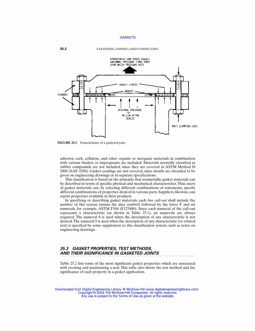
asbestos, cork, cellulose, and other organic or inorganic materials in combinationwith various binders or impregnants are included. Materials normally classified asrubber compounds are not included, since they are covered in ASTM Method D2000 (SAE J200). Gasket coatings are not covered, since details are intended to begiven on engineering drawings or in separate specifications.
This classification is based on the principle that nonmetallic gasket materials canbe described in terms of specific physical and mechanical characteristics. Thus, usersof gasket materials can, by selecting different combinations of statements, specifydifferent combinations of properties desired in various parts. Suppliers, likewise, canreport properties available in their products.
In specifying or describing gasket materials, each line call-out shall include thenumber of this system (minus the date symbol) followed by the letter F and sixnumerals, for example, ASTM F104 (F125400). Since each numeral of the call-outrepresents a characteristic (as shown in Table 25.1), six numerals are alwaysrequired. The numeral 0 is used when the description of any characteristic is notdesired. The numeral 9 is used when the description of any characteristic (or relatedtest) is specified by some supplement to this classification system, such as notes onengineering drawings.
25.3 GASKET PROPERTIES, TEST METHODS,AND THEIR SIGNIFICANCE IN GASKETED JOINTS
Table 25.2 lists some of the most significant gasket properties which are associatedwith creating and maintaining a seal. This table also shows the test method and thesignificance of each property in a gasket application.
25.2 FASTENING, JOINING, AND CONNECTING
FIGURE 25.1 Nomenclature of a gasketed joint.
GASKETS
Downloaded from Digital Engineering Library @ McGraw-Hill (www.digitalengineeringlibrary.com)Copyright © 2004 The McGraw-Hill Companies. All rights reserved.
Any use is subject to the Terms of Use as given at the website.
25.4 PERMEABILITY PROPERTIES
For a material to be impervious to a fluid, a sufficient density to eliminate voidswhich might allow capillary flow of the fluid through the construction must beachieved. This requirement may be met in two ways: by compressing the material tofill the voids and/or by partially or completely filling them during fabrication bymeans of binders and fillers.Also, for the material to maintain its impermeability fora prolonged time, its constituents must be able to resist degradation and disintegra-tion resulting from chemical attack and temperature of the application [25.2].
Most gasket materials are composed of a fibrous or granular base material, form-ing a basic matrix or foundation, which is held together or strengthened with abinder.The choice of combinations of binder and base material depends on the com-patibility of the components, the conditions of the sealing environment, and theload-bearing properties required for the application.
Some of the major constituents and the properties which are related to imper-meability are listed here.
25.4.1 Base Materials—Nonmetallic
Cork and Cork-Rubber. High compressibility allows easy density increase of thematerial, thus enabling an effective seal at low flange pressures. The temperaturelimit is approximately 250°F (121°C) for cork and 300°F (149°C) for cork-rubbercompositions. Chemical resistance to water, oil, and solvents is good, but resistanceto inorganic acids, alkalies, and oxidizing environments is poor.These materials con-form well to distorted flanges.
Cellulose Fiber. Cellulose has good chemical resistance to most fluids exceptstrong acids and bases. The temperature limitation is approximately 300°F (149°C).Changes in humidity may result in dimensional changes and/or hardening.
Asbestos Fiber. This material has good heat resistance to 800°F (427°C) and isnoncombustible. It is almost chemically inert (crocidolite fibers, commonly knownas blue asbestos, resist even inorganic acids) and has very low compressibility. Thebinder dictates the resistance to temperature and the medium to be sealed.
Nonasbestos Fibers. A number of nonasbestos fibers are being used in gaskets.Some of these are glass, carbon, aramid, and ceramic.These fibers are expensive andare normally used only in small amounts. Temperature limits from 750 to 2400°F(399 to 1316°C) are obtainable. Use of these fillers is an emerging field today, andsuppliers should be contacted before these fibers are specified for use.
25.4.2 Binders and Fillers
Rubber. Rubber binders provide varying temperature and chemical resistancedepending on the type of rubber used. These rubber and rubberlike materials areused as binders and, in some cases, gaskets:
1. Natural This rubber has good mechanical properties and is impervious towater and air. It has uncontrolled swell in petroleum oil and fuel and chlori-nated solvents. The temperature limit is 250°F (121°C).
GASKETS 25.3
GASKETS
Downloaded from Digital Engineering Library @ McGraw-Hill (www.digitalengineeringlibrary.com)Copyright © 2004 The McGraw-Hill Companies. All rights reserved.
Any use is subject to the Terms of Use as given at the website.

25.4 FASTENING, JOINING, AND CONNECTING
TABLE 25.1 Basic Physical and Mechanical Characteristics
GASKETS
Downloaded from Digital Engineering Library @ McGraw-Hill (www.digitalengineeringlibrary.com)Copyright © 2004 The McGraw-Hill Companies. All rights reserved.
Any use is subject to the Terms of Use as given at the website.
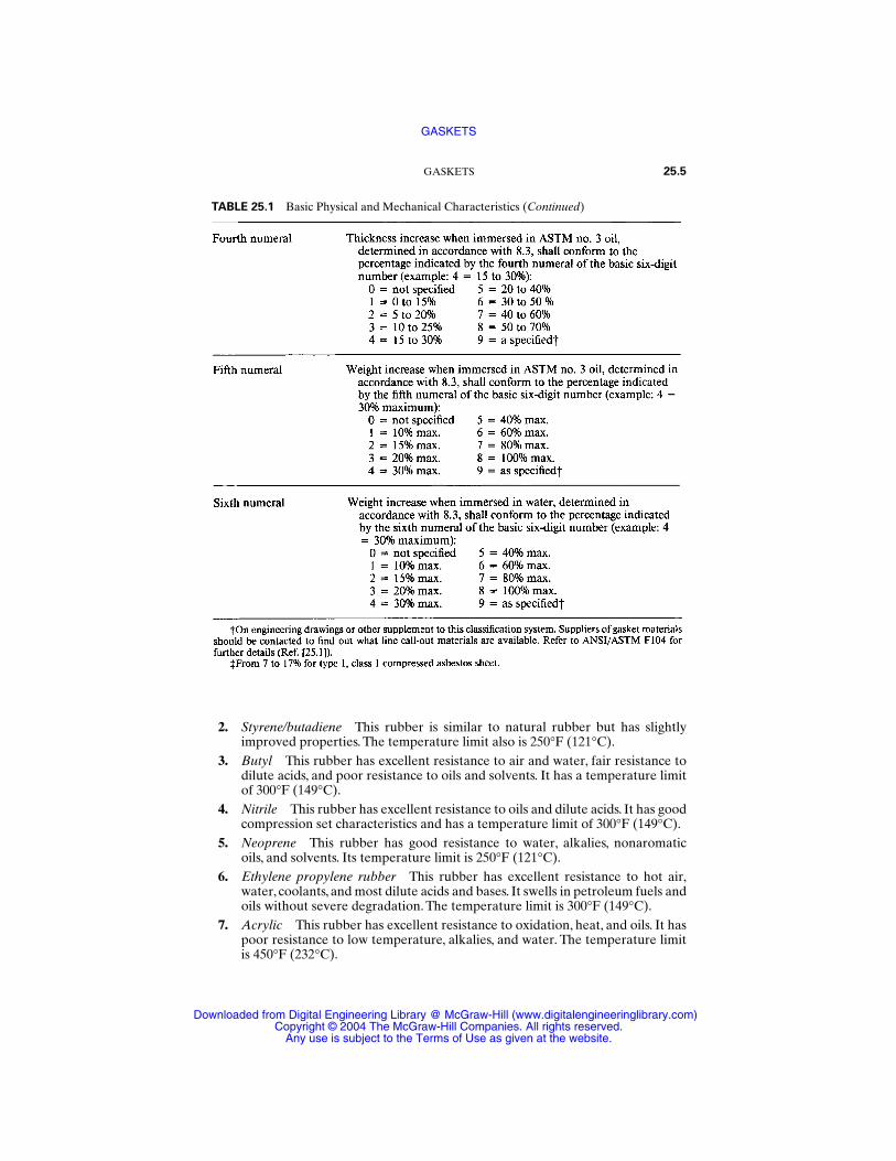
2. Styrene/butadiene This rubber is similar to natural rubber but has slightlyimproved properties. The temperature limit also is 250°F (121°C).
3. Butyl This rubber has excellent resistance to air and water, fair resistance todilute acids, and poor resistance to oils and solvents. It has a temperature limitof 300°F (149°C).
4. Nitrile This rubber has excellent resistance to oils and dilute acids. It has goodcompression set characteristics and has a temperature limit of 300°F (149°C).
5. Neoprene This rubber has good resistance to water, alkalies, nonaromaticoils, and solvents. Its temperature limit is 250°F (121°C).
6. Ethylene propylene rubber This rubber has excellent resistance to hot air,water, coolants, and most dilute acids and bases. It swells in petroleum fuels andoils without severe degradation. The temperature limit is 300°F (149°C).
7. Acrylic This rubber has excellent resistance to oxidation, heat, and oils. It haspoor resistance to low temperature, alkalies, and water. The temperature limitis 450°F (232°C).
GASKETS 25.5
TABLE 25.1 Basic Physical and Mechanical Characteristics (Continued)
GASKETS
Downloaded from Digital Engineering Library @ McGraw-Hill (www.digitalengineeringlibrary.com)Copyright © 2004 The McGraw-Hill Companies. All rights reserved.
Any use is subject to the Terms of Use as given at the website.

8. Silicone This rubber has good heat stability and low-temperature flexibility. It isnot suitable for high mechanical pressure. Its temperature limit is 600°F (316°C).
9. Viton This rubber has good resistance to oils, fuel, and chlorinated solvents. Italso has excellent low-temperature properties. Its temperature limit is 600°F(316°C).
10. Fluorocarbon This rubber has excellent resistance to most fluids, except syn-thetic lubricants. The temperature limit is 500°F (260°C).
Resins. These usually possess better chemical resistance than rubber.Temperaturelimitations depend on whether the resin is thermosetting or thermoplastic.
Tanned Glue and Glycerine. This combination produces a continuous gel struc-ture throughout the material, allowing sealing at low flange loading. It has goodchemical resistance to most oils, fuels, and solvents. It swells in water but is not solu-ble. The temperature limit is 200°F (93°C). It is used as a saturant in cellulose paper.
Fillers. In some cases, inert fillers are added to the material composition to aid infilling voids. Some examples are barytes, asbestine, and cork dust.
25.4.3 Reinforcements
Some of the properties of nonmetallic gasket materials can be improved if the gas-kets are reinforced with metal or fabric cores. Major improvements in torque reten-tion and blowout resistance are normally seen. Traditionally, perforated or upsetmetal cores have been used to support gasket facings. A number of designs havebeen utilized for production. Size of the perforations and their frequency in a givenarea are the usual specified parameters.
25.6 FASTENING, JOINING, AND CONNECTING
TABLE 25.2 Identification, Test Method, and Significance of Various Properties Associatedwith Gasket Materials
GASKETS
Downloaded from Digital Engineering Library @ McGraw-Hill (www.digitalengineeringlibrary.com)Copyright © 2004 The McGraw-Hill Companies. All rights reserved.
Any use is subject to the Terms of Use as given at the website.
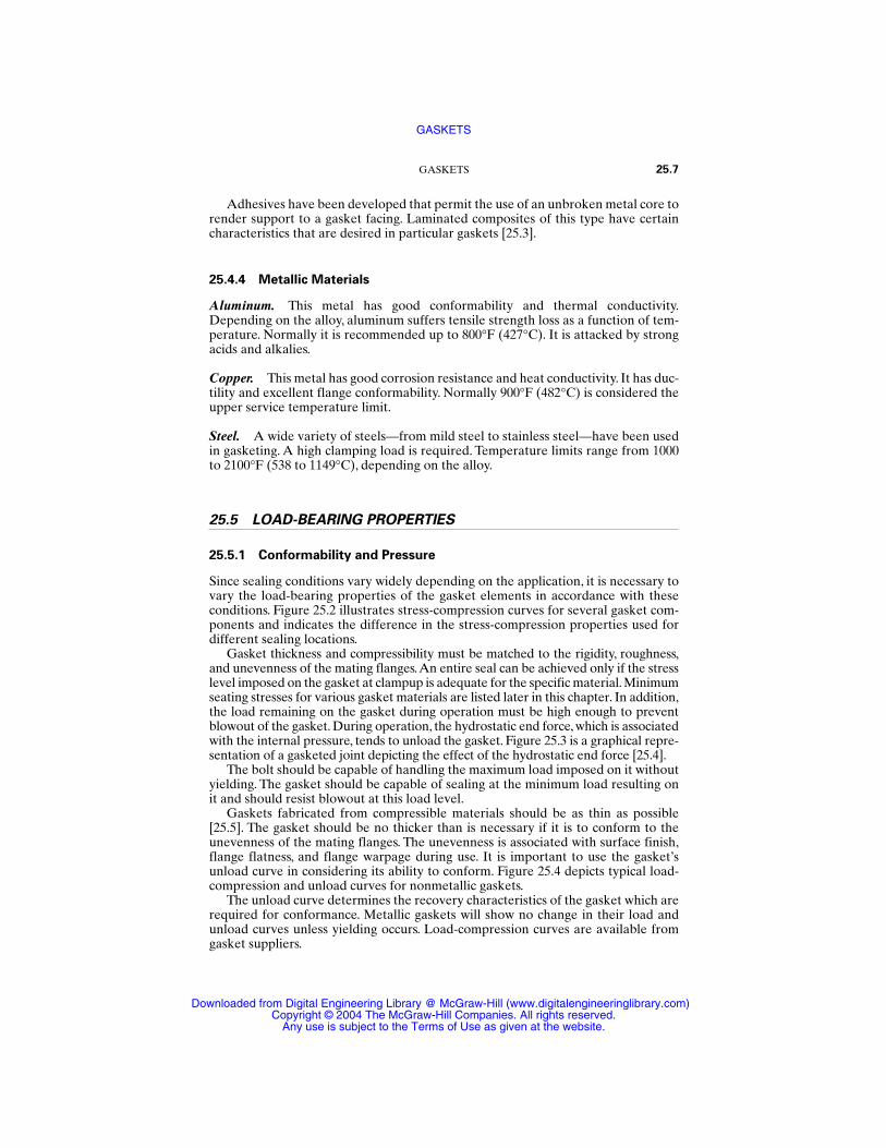
Adhesives have been developed that permit the use of an unbroken metal core torender support to a gasket facing. Laminated composites of this type have certaincharacteristics that are desired in particular gaskets [25.3].
25.4.4 Metallic Materials
Aluminum. This metal has good conformability and thermal conductivity.Depending on the alloy, aluminum suffers tensile strength loss as a function of tem-perature. Normally it is recommended up to 800°F (427°C). It is attacked by strongacids and alkalies.
Copper. This metal has good corrosion resistance and heat conductivity. It has duc-tility and excellent flange conformability. Normally 900°F (482°C) is considered theupper service temperature limit.
Steel. A wide variety of steels—from mild steel to stainless steel—have been usedin gasketing. A high clamping load is required. Temperature limits range from 1000to 2100°F (538 to 1149°C), depending on the alloy.
25.5 LOAD-BEARING PROPERTIES
25.5.1 Conformability and Pressure
Since sealing conditions vary widely depending on the application, it is necessary tovary the load-bearing properties of the gasket elements in accordance with theseconditions. Figure 25.2 illustrates stress-compression curves for several gasket com-ponents and indicates the difference in the stress-compression properties used fordifferent sealing locations.
Gasket thickness and compressibility must be matched to the rigidity, roughness,and unevenness of the mating flanges.An entire seal can be achieved only if the stresslevel imposed on the gasket at clampup is adequate for the specific material. Minimumseating stresses for various gasket materials are listed later in this chapter. In addition,the load remaining on the gasket during operation must be high enough to preventblowout of the gasket. During operation, the hydrostatic end force, which is associatedwith the internal pressure, tends to unload the gasket. Figure 25.3 is a graphical repre-sentation of a gasketed joint depicting the effect of the hydrostatic end force [25.4].
The bolt should be capable of handling the maximum load imposed on it withoutyielding. The gasket should be capable of sealing at the minimum load resulting onit and should resist blowout at this load level.
Gaskets fabricated from compressible materials should be as thin as possible[25.5]. The gasket should be no thicker than is necessary if it is to conform to theunevenness of the mating flanges. The unevenness is associated with surface finish,flange flatness, and flange warpage during use. It is important to use the gasket’sunload curve in considering its ability to conform. Figure 25.4 depicts typical load-compression and unload curves for nonmetallic gaskets.
The unload curve determines the recovery characteristics of the gasket which arerequired for conformance. Metallic gaskets will show no change in their load andunload curves unless yielding occurs. Load-compression curves are available fromgasket suppliers.
GASKETS 25.7
GASKETS
Downloaded from Digital Engineering Library @ McGraw-Hill (www.digitalengineeringlibrary.com)Copyright © 2004 The McGraw-Hill Companies. All rights reserved.
Any use is subject to the Terms of Use as given at the website.
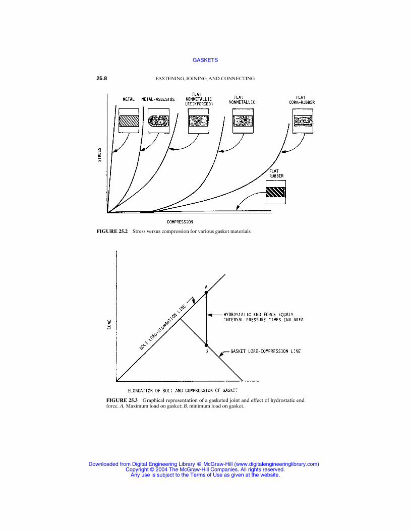
25.8 FASTENING, JOINING, AND CONNECTING
FIGURE 25.2 Stress versus compression for various gasket materials.
FIGURE 25.3 Graphical representation of a gasketed joint and effect of hydrostatic endforce. A, Maximum load on gasket; B, minimum load on gasket.
GASKETS
Downloaded from Digital Engineering Library @ McGraw-Hill (www.digitalengineeringlibrary.com)Copyright © 2004 The McGraw-Hill Companies. All rights reserved.
Any use is subject to the Terms of Use as given at the website.
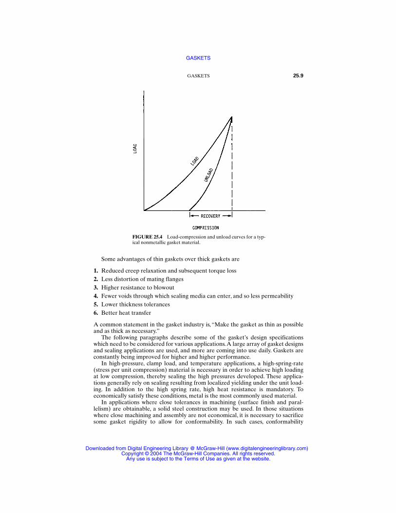
Some advantages of thin gaskets over thick gaskets are
1. Reduced creep relaxation and subsequent torque loss2. Less distortion of mating flanges3. Higher resistance to blowout4. Fewer voids through which sealing media can enter, and so less permeability5. Lower thickness tolerances6. Better heat transfer
A common statement in the gasket industry is, “Make the gasket as thin as possibleand as thick as necessary.”
The following paragraphs describe some of the gasket’s design specificationswhich need to be considered for various applications.A large array of gasket designsand sealing applications are used, and more are coming into use daily. Gaskets areconstantly being improved for higher and higher performance.
In high-pressure, clamp load, and temperature applications, a high-spring-rate(stress per unit compression) material is necessary in order to achieve high loadingat low compression, thereby sealing the high pressures developed. These applica-tions generally rely on sealing resulting from localized yielding under the unit load-ing. In addition to the high spring rate, high heat resistance is mandatory. Toeconomically satisfy these conditions, metal is the most commonly used material.
In applications where close tolerances in machining (surface finish and paral-lelism) are obtainable, a solid steel construction may be used. In those situationswhere close machining and assembly are not economical, it is necessary to sacrificesome gasket rigidity to allow for conformability. In such cases, conformability
GASKETS 25.9
FIGURE 25.4 Load-compression and unload curves for a typ-ical nonmetallic gasket material.
GASKETS
Downloaded from Digital Engineering Library @ McGraw-Hill (www.digitalengineeringlibrary.com)Copyright © 2004 The McGraw-Hill Companies. All rights reserved.
Any use is subject to the Terms of Use as given at the website.
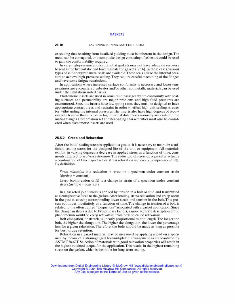
exceeding that resulting from localized yielding must be inherent in the design. Themetal can be corrugated, or a composite design consisting of asbestos could be usedto gain the conformability required.
In very-high-pressure applications, flat gaskets may not have adequate recoveryto seal as the hydrostatic end force unseats the gaskets [25.6]. In these cases, varioustypes of self-energized metal seals are available.These seals utilize the internal pres-sure to achieve high-pressure sealing. They require careful machining of the flangesand have some fatigue restrictions.
In applications where increased surface conformity is necessary and lower tem-peratures are encountered, asbestos and/or other nonmetallic materials can be usedunder the limitations noted earlier.
Elastomeric inserts are used in some fluid passages where conformity with seal-ing surfaces and permeability are major problems and high fluid pressures areencountered. Since the inserts have low spring rates, they must be designed to haveappropriate contact areas and restraint in order to effect high unit sealing stressesfor withstanding the internal pressures. The inserts also have high degrees of recov-ery, which allow them to follow high thermal distortions normally associated in themating flanges. Compression set and heat-aging characteristics must also be consid-ered when elastomeric inserts are used.
25.5.2 Creep and Relaxation
After the initial sealing stress is applied to a gasket, it is necessary to maintain a suf-ficient sealing stress for the designed life of the unit or equipment. All materialsexhibit, in varying degrees, a decrease in applied stress as a function of time, com-monly referred to as stress relaxation. The reduction of stress on a gasket is actuallya combination of two major factors: stress relaxation and creep (compression drift).By definition,
Stress relaxation is a reduction in stress on a specimen under constant strain(dσ/dt; e = constant).Creep (compression drift) is a change in strain of a specimen under constantstress (de/dt; σ = constant).
In a gasketed joint, stress is applied by tension in a bolt or stud and transmittedas a compressive force to the gasket.After loading, stress relaxation and creep occurin the gasket, causing corresponding lower strain and tension in the bolt. This pro-cess continues indefinitely as a function of time. The change in tension of a bolt isrelated to the often quoted “torque loss” associated with a gasket application. Sincethe change in stress is due to two primary factors, a more accurate description of thephenomenon would be creep relaxation, from now on called relaxation.
Bolt elongation, or stretch, is linearly proportional to bolt length. The longer thebolt, the higher the elongation. The higher the elongation, the lower the percentageloss for a given relaxation. Therefore, the bolts should be made as long as possiblefor best torque retention.
Relaxation in a gasket material may be measured by applying a load on a speci-men by means of a strain-gauged bolt-nut-platen arrangement as standardized byASTM F38-62T. Selection of materials with good relaxation properties will result inthe highest retained torque for the application. This results in the highest remainingstress on the gasket, which is desirable for long-term sealing.
25.10 FASTENING, JOINING, AND CONNECTING
GASKETS
Downloaded from Digital Engineering Library @ McGraw-Hill (www.digitalengineeringlibrary.com)Copyright © 2004 The McGraw-Hill Companies. All rights reserved.
Any use is subject to the Terms of Use as given at the website.
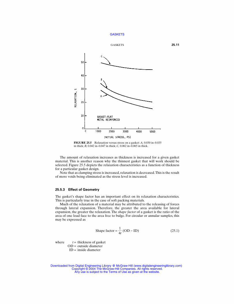
The amount of relaxation increases as thickness is increased for a given gasketmaterial. This is another reason why the thinnest gasket that will work should beselected. Figure 25.5 depicts the relaxation characteristics as a function of thicknessfor a particular gasket design.
Note that as clamping stress is increased, relaxation is decreased.This is the resultof more voids being eliminated as the stress level is increased.
25.5.3 Effect of Geometry
The gasket’s shape factor has an important effect on its relaxation characteristics.This is particularly true in the case of soft packing materials.
Much of the relaxation of a material may be attributed to the releasing of forcesthrough lateral expansion. Therefore, the greater the area available for lateralexpansion, the greater the relaxation. The shape factor of a gasket is the ratio of thearea of one load face to the area free to bulge. For circular or annular samples, thismay be expressed as
Shape factor = (OD − ID) (25.1)
where t = thickness of gasketOD = outside diameterID = inside diameter
14t
GASKETS 25.11
FIGURE 25.5 Relaxation versus stress on a gasket: A, 0.030 in–0.035in thick; B, 0.042 in–0.047 in thick; C, 0.062 in–0.065 in thick.
GASKETS
Downloaded from Digital Engineering Library @ McGraw-Hill (www.digitalengineeringlibrary.com)Copyright © 2004 The McGraw-Hill Companies. All rights reserved.
Any use is subject to the Terms of Use as given at the website.
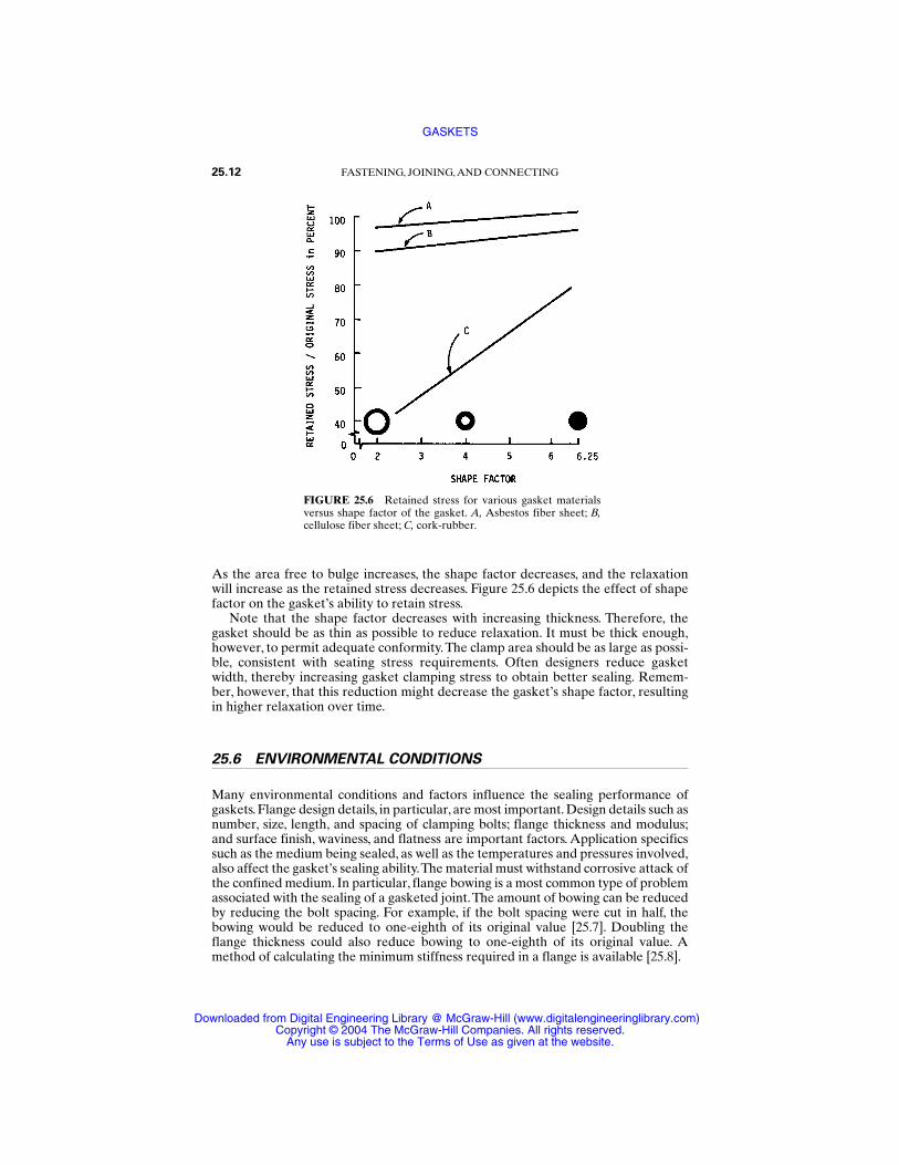
As the area free to bulge increases, the shape factor decreases, and the relaxationwill increase as the retained stress decreases. Figure 25.6 depicts the effect of shapefactor on the gasket’s ability to retain stress.
Note that the shape factor decreases with increasing thickness. Therefore, thegasket should be as thin as possible to reduce relaxation. It must be thick enough,however, to permit adequate conformity.The clamp area should be as large as possi-ble, consistent with seating stress requirements. Often designers reduce gasketwidth, thereby increasing gasket clamping stress to obtain better sealing. Remem-ber, however, that this reduction might decrease the gasket’s shape factor, resultingin higher relaxation over time.
25.6 ENVIRONMENTAL CONDITIONS
Many environmental conditions and factors influence the sealing performance ofgaskets. Flange design details, in particular, are most important. Design details such asnumber, size, length, and spacing of clamping bolts; flange thickness and modulus;and surface finish, waviness, and flatness are important factors. Application specificssuch as the medium being sealed, as well as the temperatures and pressures involved,also affect the gasket’s sealing ability.The material must withstand corrosive attack ofthe confined medium. In particular, flange bowing is a most common type of problemassociated with the sealing of a gasketed joint.The amount of bowing can be reducedby reducing the bolt spacing. For example, if the bolt spacing were cut in half, thebowing would be reduced to one-eighth of its original value [25.7]. Doubling theflange thickness could also reduce bowing to one-eighth of its original value. Amethod of calculating the minimum stiffness required in a flange is available [25.8].
25.12 FASTENING, JOINING, AND CONNECTING
FIGURE 25.6 Retained stress for various gasket materialsversus shape factor of the gasket. A, Asbestos fiber sheet; B,cellulose fiber sheet; C, cork-rubber.
GASKETS
Downloaded from Digital Engineering Library @ McGraw-Hill (www.digitalengineeringlibrary.com)Copyright © 2004 The McGraw-Hill Companies. All rights reserved.
Any use is subject to the Terms of Use as given at the website.
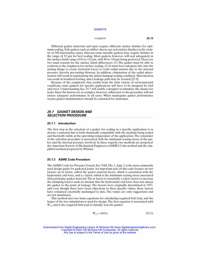
Different gasket materials and types require different surface finishes for opti-mum sealing. Soft gaskets such as rubber sheets can seal surface finishes in the vicin-ity of 500 microinches (µin), whereas some metallic gaskets may require finishes inthe range of 32 µin for best sealing. Most gaskets, however, will seal adequately inthe surface finish range of 63 to 125 µin, with 90 to 110 µin being preferred.There aretwo main reasons for the surface finish differences: (1) The gasket must be able toconform to the roughness for surface sealing. (2) It must have adequate bite into themating flange to create frictional forces to resist radial motion due to the internalpressure, thereby preventing blowout. In addition, elimination of the radial micro-motion will result in maintaining the initial clampup sealing condition. Micromotioncan result in localized fretting, and a leakage path may be created [25.9].
Because of the complexity that results from the wide variety of environmentalconditions, some gaskets for specific applications will have to be designed by trialand error. Understanding Sec. 25.7 will enable a designer to minimize the chance forleaks. Since the factors are so complex, however, adherence to the procedure will notensure adequate performance in all cases. When inadequate gasket performanceoccurs, gasket manufacturers should be contacted for assistance.
25.7 GASKET DESIGN AND SELECTION PROCEDURE
25.7.1 Introduction
The first step in the selection of a gasket for sealing in a specific application is tochoose a material that is both chemically compatible with the medium being sealedand thermally stable at the operating temperature of the application.The remainderof the selection procedure is associated with the minimum seating stress of the gas-ket and the internal pressure involved. In these regards, two methods are proposed:the American Society of Mechanical Engineers (ASME) Code method and the sim-plified method proposed by Whalen.
25.7.2 ASME Code Procedure
The ASME Code for Pressure Vessels, Sec.VIII, Div. 1,App. 2, is the most commonlyused design guide for gasketed joints. An important part of this code focuses on twofactors: an m factor, called the gasket material factor, which is associated with thehydrostatic end force, and a y factor, which is the minimum seating stress associatedwith particular gasket material. The m factor is essentially a safety factor to increasethe clamping load to such an amount that the hydrostatic end force does not unseatthe gasket to the point of leakage. The factors were originally determined in 1937,and even though there have been objections to their specific values, these factorshave remained essentially unchanged to date. The values are only suggestions andare not mandatory.
This method uses two basic equations for calculating required bolt load, and thelarger of the two calculations is used for design. The first equation is associated withWm2 and is the required bolt load to initially seat the gasket:
Wm2 = πbGy (25.2)
GASKETS 25.13
GASKETS
Downloaded from Digital Engineering Library @ McGraw-Hill (www.digitalengineeringlibrary.com)Copyright © 2004 The McGraw-Hill Companies. All rights reserved.
Any use is subject to the Terms of Use as given at the website.
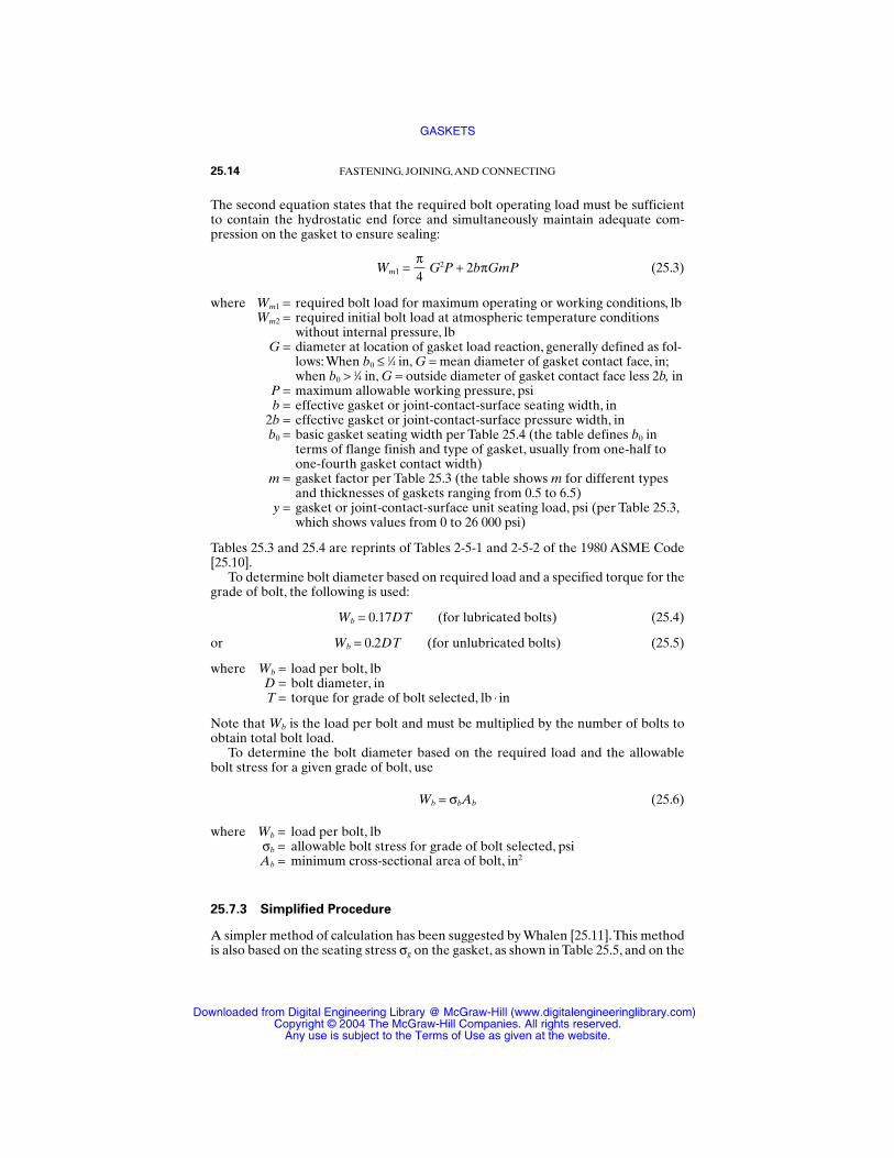
The second equation states that the required bolt operating load must be sufficientto contain the hydrostatic end force and simultaneously maintain adequate com-pression on the gasket to ensure sealing:
Wm1 = G2P + 2bπGmP (25.3)
where Wm1 = required bolt load for maximum operating or working conditions, lbWm2 = required initial bolt load at atmospheric temperature conditions
without internal pressure, lbG = diameter at location of gasket load reaction, generally defined as fol-
lows: When b0 ≤ 1⁄4 in, G = mean diameter of gasket contact face, in;when b0 > 1⁄4 in, G = outside diameter of gasket contact face less 2b, in
P = maximum allowable working pressure, psib = effective gasket or joint-contact-surface seating width, in
2b = effective gasket or joint-contact-surface pressure width, inb0 = basic gasket seating width per Table 25.4 (the table defines b0 in
terms of flange finish and type of gasket, usually from one-half toone-fourth gasket contact width)
m = gasket factor per Table 25.3 (the table shows m for different typesand thicknesses of gaskets ranging from 0.5 to 6.5)
y = gasket or joint-contact-surface unit seating load, psi (per Table 25.3,which shows values from 0 to 26 000 psi)
Tables 25.3 and 25.4 are reprints of Tables 2-5-1 and 2-5-2 of the 1980 ASME Code[25.10].
To determine bolt diameter based on required load and a specified torque for thegrade of bolt, the following is used:
Wb = 0.17DT (for lubricated bolts) (25.4)
or Wb = 0.2DT (for unlubricated bolts) (25.5)
where Wb = load per bolt, lbD = bolt diameter, inT = torque for grade of bolt selected, lb ⋅ in
Note that Wb is the load per bolt and must be multiplied by the number of bolts toobtain total bolt load.
To determine the bolt diameter based on the required load and the allowablebolt stress for a given grade of bolt, use
Wb = σbAb (25.6)
where Wb = load per bolt, lbσb = allowable bolt stress for grade of bolt selected, psiAb = minimum cross-sectional area of bolt, in2
25.7.3 Simplified Procedure
A simpler method of calculation has been suggested by Whalen [25.11].This methodis also based on the seating stress σg on the gasket, as shown in Table 25.5, and on the
π4
25.14 FASTENING, JOINING, AND CONNECTING
GASKETS
Downloaded from Digital Engineering Library @ McGraw-Hill (www.digitalengineeringlibrary.com)Copyright © 2004 The McGraw-Hill Companies. All rights reserved.
Any use is subject to the Terms of Use as given at the website.
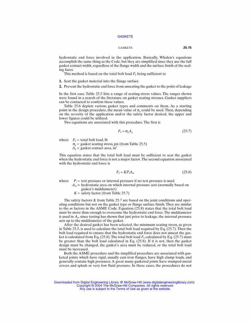
hydrostatic end force involved in the application. Basically, Whalen’s equationsaccomplish the same thing as the Code, but they are simplified since they use the fullgasket contact width, regardless of the flange width and the surface finish of the seal-ing faces.
This method is based on the total bolt load Fb being sufficient to
1. Seat the gasket material into the flange surface2. Prevent the hydrostatic end force from unseating the gasket to the point of leakage
In the first case, Table 25.5 lists a range of seating-stress values. The ranges shownwere found in a search of the literature on gasket seating stresses. Gasket supplierscan be contacted to confirm these values.
Table 25.6 depicts various gasket types and comments on them. As a startingpoint in the design procedure, the mean value of σg could be used. Then, dependingon the severity of the application and/or the safety factor desired, the upper andlower figures could be utilized.
Two equations are associated with this procedure. The first is
Fb = σgAg (25.7)
where Fb = total bolt load, lbσg = gasket seating stress, psi (from Table 25.5)Ag = gasket contact area, in2
This equation states that the total bolt load must be sufficient to seat the gasketwhen the hydrostatic end force is not a major factor.The second equation associatedwith the hydrostatic end force is
Fb = KPtAm (25.8)
where Pt = test pressure or internal pressure if no test pressure is usedAm = hydrostatic area on which internal pressure acts (normally based on
gasket’s middiameter)K = safety factor (from Table 25.7)
The safety factors K from Table 25.7 are based on the joint conditions and oper-ating conditions but not on the gasket type or flange surface finish. They are similarto the m factors in the ASME Code. Equation (25.8) states that the total bolt loadmust be more than enough to overcome the hydrostatic end force. The middiameteris used in Am since testing has shown that just prior to leakage, the internal pressureacts up to the middiameter of the gasket.
After the desired gasket has been selected, the minimum seating stress, as givenin Table 25.5, is used to calculate the total bolt load required by Eq. (25.7). Then thebolt load required to ensure that the hydrostatic end force does not unseat the gas-ket is calculated from Eq. (25.8).The total bolt load Fb calculated by Eq. (25.7) mustbe greater than the bolt load calculated in Eq. (25.8). If it is not, then the gasketdesign must be changed, the gasket’s area must be reduced, or the total bolt loadmust be increased.
Both the ASME procedure and the simplified procedure are associated with gas-keted joints which have rigid, usually cast-iron flanges, have high clamp loads, andgenerally contain high pressures. A great many gasketed joints have stamped-metalcovers and splash or very low fluid pressure. In these cases, the procedures do not
GASKETS 25.15
GASKETS
Downloaded from Digital Engineering Library @ McGraw-Hill (www.digitalengineeringlibrary.com)Copyright © 2004 The McGraw-Hill Companies. All rights reserved.
Any use is subject to the Terms of Use as given at the website.
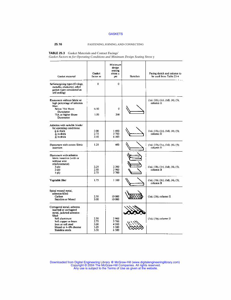
25.16 FASTENING, JOINING, AND CONNECTING
TABLE 25.3 Gasket Materials and Contact Facings†
Gasket Factors m for Operating Conditions and Minimum Design Seating Stress y
GASKETS
Downloaded from Digital Engineering Library @ McGraw-Hill (www.digitalengineeringlibrary.com)Copyright © 2004 The McGraw-Hill Companies. All rights reserved.
Any use is subject to the Terms of Use as given at the website.
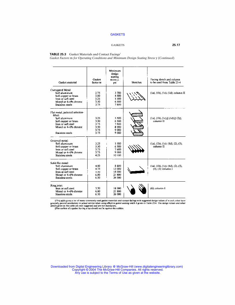
GASKETS 25.17
TABLE 25.3 Gasket Materials and Contact Facings†
Gasket Factors m for Operating Conditions and Minimum Design Seating Stress y (Continued)
GASKETS
Downloaded from Digital Engineering Library @ McGraw-Hill (www.digitalengineeringlibrary.com)Copyright © 2004 The McGraw-Hill Companies. All rights reserved.
Any use is subject to the Terms of Use as given at the website.
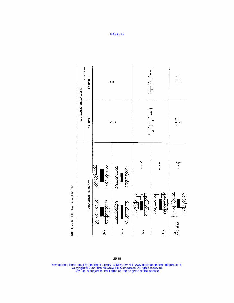
TA
BLE
25.4
Eff
ecti
ve G
aske
t Wid
th†
25.18
GASKETS
Downloaded from Digital Engineering Library @ McGraw-Hill (www.digitalengineeringlibrary.com)Copyright © 2004 The McGraw-Hill Companies. All rights reserved.
Any use is subject to the Terms of Use as given at the website.
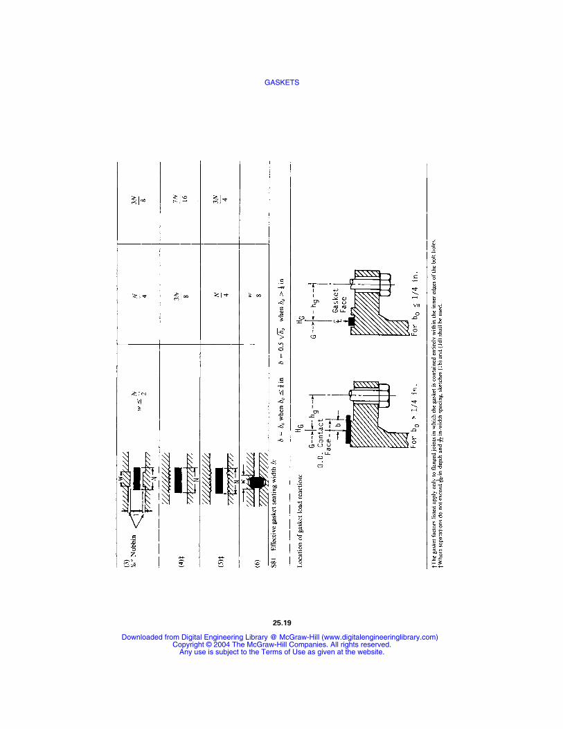
25.19
GASKETS
Downloaded from Digital Engineering Library @ McGraw-Hill (www.digitalengineeringlibrary.com)Copyright © 2004 The McGraw-Hill Companies. All rights reserved.
Any use is subject to the Terms of Use as given at the website.

25.20 FASTENING, JOINING, AND CONNECTING
TABLE 25.5 Minimum Recommended Seating Stresses for Various Gasket Materials
GASKETS
Downloaded from Digital Engineering Library @ McGraw-Hill (www.digitalengineeringlibrary.com)Copyright © 2004 The McGraw-Hill Companies. All rights reserved.
Any use is subject to the Terms of Use as given at the website.
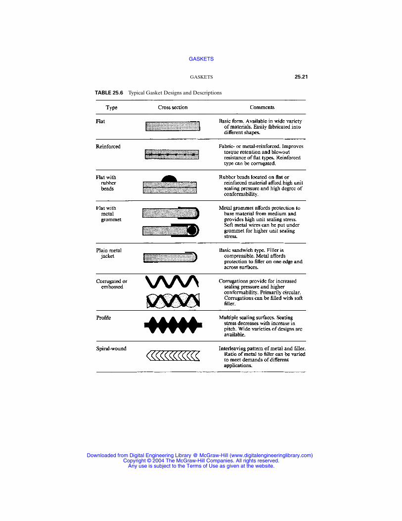
GASKETS 25.21
TABLE 25.6 Typical Gasket Designs and Descriptions
GASKETS
Downloaded from Digital Engineering Library @ McGraw-Hill (www.digitalengineeringlibrary.com)Copyright © 2004 The McGraw-Hill Companies. All rights reserved.
Any use is subject to the Terms of Use as given at the website.
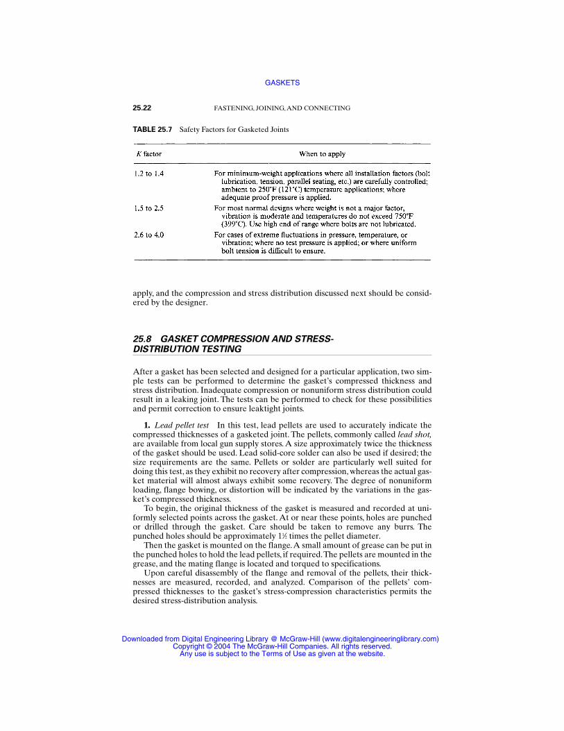
apply, and the compression and stress distribution discussed next should be consid-ered by the designer.
25.8 GASKET COMPRESSION AND STRESS-DISTRIBUTION TESTING
After a gasket has been selected and designed for a particular application, two sim-ple tests can be performed to determine the gasket’s compressed thickness andstress distribution. Inadequate compression or nonuniform stress distribution couldresult in a leaking joint. The tests can be performed to check for these possibilitiesand permit correction to ensure leaktight joints.
1. Lead pellet test In this test, lead pellets are used to accurately indicate thecompressed thicknesses of a gasketed joint. The pellets, commonly called lead shot,are available from local gun supply stores. A size approximately twice the thicknessof the gasket should be used. Lead solid-core solder can also be used if desired; thesize requirements are the same. Pellets or solder are particularly well suited fordoing this test, as they exhibit no recovery after compression, whereas the actual gas-ket material will almost always exhibit some recovery. The degree of nonuniformloading, flange bowing, or distortion will be indicated by the variations in the gas-ket’s compressed thickness.
To begin, the original thickness of the gasket is measured and recorded at uni-formly selected points across the gasket. At or near these points, holes are punchedor drilled through the gasket. Care should be taken to remove any burrs. Thepunched holes should be approximately 11⁄2 times the pellet diameter.
Then the gasket is mounted on the flange.A small amount of grease can be put inthe punched holes to hold the lead pellets, if required.The pellets are mounted in thegrease, and the mating flange is located and torqued to specifications.
Upon careful disassembly of the flange and removal of the pellets, their thick-nesses are measured, recorded, and analyzed. Comparison of the pellets’ com-pressed thicknesses to the gasket’s stress-compression characteristics permits thedesired stress-distribution analysis.
25.22 FASTENING, JOINING, AND CONNECTING
TABLE 25.7 Safety Factors for Gasketed Joints
GASKETS
Downloaded from Digital Engineering Library @ McGraw-Hill (www.digitalengineeringlibrary.com)Copyright © 2004 The McGraw-Hill Companies. All rights reserved.
Any use is subject to the Terms of Use as given at the website.
2. NCR paper test This test utilizes no-carbon-required (NCR) paper forvisual determination of the stress distribution on a gasket. NCR paper is a pressure-sensitive, color-reactive paper. The intensity of color is proportional to the stressimposed on the paper, which is the same as the stress on the gasket.
NCR paper is available from the NCR Corp., the 3M Company, and other papercompanies. Various grades are available, but the medium grade is usually chosen.Some papers are only one sheet, whereas others are composed of two sheets. Eithertype can be used.
To begin, the bolt holes are pierced in a piece of the impression paper. Thepierced holes in the paper are made slightly larger than the bolts.The paper is placedon the flange, and the mating flange is assembled per torque specifications.
When you are using the two-piece carbonless paper, make sure to keep the twopapers oriented to each other as they were purchased; otherwise, no impression mayresult. Upon torquing, the impression is made on the paper. The flange is removed,and the impression is inspected for stress distribution. A judgment of the gasket’ssealing ability can now be made. Further analysis can be done by calibrating the loadversus the color intensity of the paper. Various known stresses can be applied to thepaper and the resulting color impressions identified. The impressions can be com-pared to the test sample, and then the stress on the sample can be determined.
In both the lead pellet and NCR paper tests, gasket manufacturers can be con-tacted for further interpretation of the results and more detailed analysis.
25.9 INSTALLATION SPECIFICATIONS
An installation is only as good as its gasket; likewise, a gasket is only as good as itsinstallation [25.1]. The following are some recommendations associated with gasketinstallation:
1. Be sure that mating surfaces are clean and in specification with regard to finish,flatness, and waviness.
2. Check gasket for damage before installing it.3. Make certain the gasket fits the application.4. Specify lubricated bolts. Bolt threads and the underside of the bolt head should
be lubricated.5. Specify the torque level.6. Specify the torquing sequence. In addition to the sequence, two or three stages of
torque before reaching the specified level are recommended.
REFERENCES
25.1 ANSI/ASTM F104-03, Standard Classification System for Nonmetallic Gasket Materials,American Society for Testing and Materials.
25.2 D. E. Czernik, J. C. Moerk, Jr., and F. A. Robbins, “The Relationship of a Gasket’s Phys-ical Properties to the Sealing Phenomena,” SAE paper 650431, May 1965.
25.3 D. E. Czernik, “Recent Developments and New Approaches in Mechanical and Chemi-cal Gasketing,” SAE paper 810367, February 1981.
GASKETS 25.23
GASKETS
Downloaded from Digital Engineering Library @ McGraw-Hill (www.digitalengineeringlibrary.com)Copyright © 2004 The McGraw-Hill Companies. All rights reserved.
Any use is subject to the Terms of Use as given at the website.
25.4 V. M. Faires, Design of Machine Elements, Macmillan, New York, 1955.
25.5 D. J. McDowell, “Choose the Right Gasket Material,” Assembly Engineering, October1978.
25.6 H. A. Rothbart, Mechanical Design and Systems Handbook, 2d ed., McGraw-Hill, NewYork, 1985, Sec. 27.4.
25.7 Armstrong Gasket Design Manual, Armstrong Cork Co., Lancaster, Pa., 1978.
25.8 J. W. Oren, “Creating Gasket Seals with Rigid Flanges,” SAE paper 810362, February1981.
25.9 D. E. Czernik, “Gasketing the Internal Combustion Engine,” SAE paper 800073, Febru-ary 1980.
25.10 The American Society of Mechanical Engineers, Code for Pressure Vessels, Sec. VIII,Div. 1, App. 2, 1980 (see 2004 edition).
25.11 J. J. Whalen, “How to Select the Right Gasket Material,” Product Engineering, October1960.
25.12 D. E. Czernik, “Sealing Today’s Engines,” Fleet Maintenance and Specifying, Irving-Cloud, July 1977.
25.24 FASTENING, JOINING, AND CONNECTING
GASKETS
Downloaded from Digital Engineering Library @ McGraw-Hill (www.digitalengineeringlibrary.com)Copyright © 2004 The McGraw-Hill Companies. All rights reserved.
Any use is subject to the Terms of Use as given at the website.

CHAPTER 26WELDED
CONNECTIONS
Richard S. SaboManager, Educational ServicesThe Lincoln Electric Company
Cleveland, Ohio
Omer W. BlodgettDesign Consultant
The Lincoln Electric CompanyCleveland, Ohio
26.1 DEFINITIONS AND TERMINOLOGY / 26.1
26.2 BASIC WELDING CIRCUIT / 26.2
26.3 ARC SHIELDING / 26.2
26.4 NATURE OF THE ARC / 26.4
26.5 OVERCOMING CURRENT LIMITATIONS / 26.5
26.6 COMMERCIAL ARC-WELDING PROCESSES / 26.6
26.7 ARC-WELDING CONSUMABLES / 26.18
26.8 DESIGN OF WELDED JOINTS / 26.23
26.9 CODES AND SPECIFICATIONS FOR WELDS / 26.39
26.1 DEFINITIONS AND TERMINOLOGY
Arc welding is one of several fusion processes for joining metals. By the applicationof intense heat, metal at the joint between two parts is melted and caused to inter-mix—directly or, more commonly, with an intermediate molten filler metal. Uponcooling and solidification, a metallurgical bond results. Since the joining is by inter-mixture of the substance of one part with the substance of the other part, with orwithout an intermediate of like substance, the final weldment has the potential forexhibiting at the joint the same strength properties as the metal of the parts. This isin sharp contrast to nonfusion processes of joining—such as soldering, brazing, oradhesive bonding—in which the mechanical and physical properties of the basematerials cannot be duplicated at the joint.
In arc welding, the intense heat needed to melt metal is produced by an electricarc. The arc is formed between the work to be welded and an electrode that is man-ually or mechanically moved along the joint (or the work may be moved under a sta-tionary electrode). The electrode may be a carbon or tungsten rod, the sole purposeof which is to carry the current and sustain the electric arc between its tip and theworkpiece. Or it may be a specially prepared rod or wire that not only conducts the
26.1
Source: STANDARD HANDBOOK OF MACHINE DESIGN
Downloaded from Digital Engineering Library @ McGraw-Hill (www.digitalengineeringlibrary.com)Copyright © 2004 The McGraw-Hill Companies. All rights reserved.
Any use is subject to the Terms of Use as given at the website.
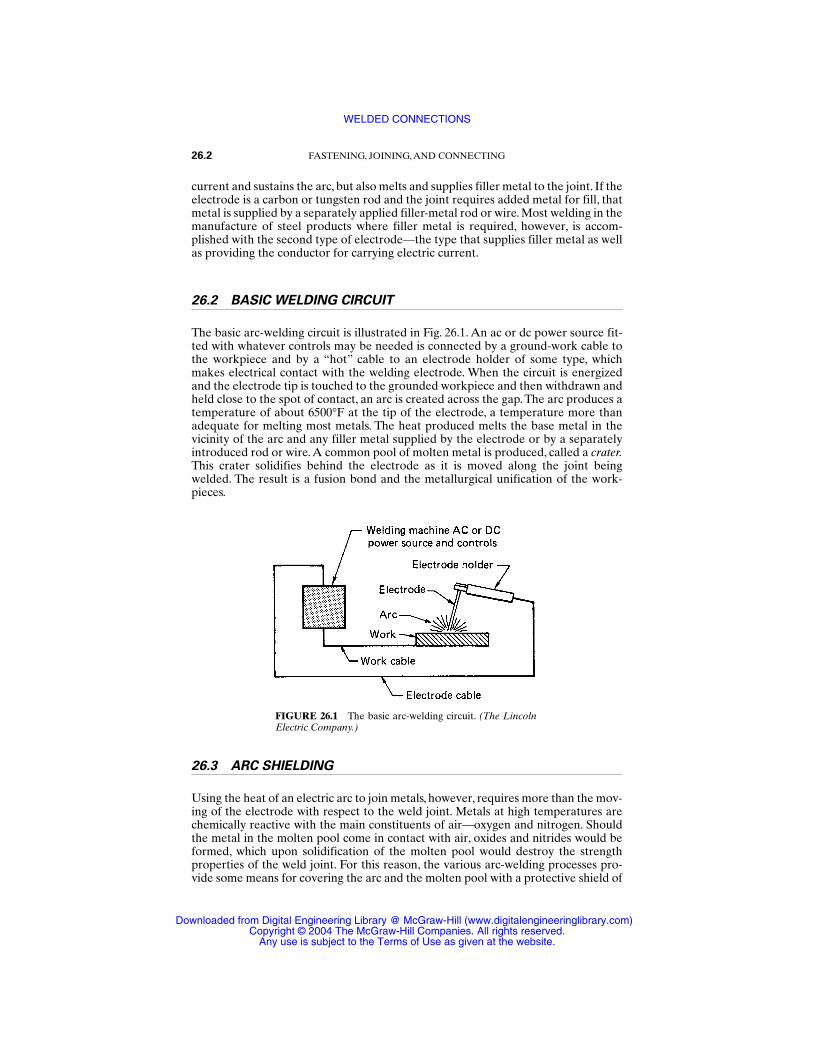
current and sustains the arc, but also melts and supplies filler metal to the joint. If theelectrode is a carbon or tungsten rod and the joint requires added metal for fill, thatmetal is supplied by a separately applied filler-metal rod or wire. Most welding in themanufacture of steel products where filler metal is required, however, is accom-plished with the second type of electrode—the type that supplies filler metal as wellas providing the conductor for carrying electric current.
26.2 BASIC WELDING CIRCUIT
The basic arc-welding circuit is illustrated in Fig. 26.1. An ac or dc power source fit-ted with whatever controls may be needed is connected by a ground-work cable tothe workpiece and by a “hot” cable to an electrode holder of some type, whichmakes electrical contact with the welding electrode. When the circuit is energizedand the electrode tip is touched to the grounded workpiece and then withdrawn andheld close to the spot of contact, an arc is created across the gap. The arc produces atemperature of about 6500°F at the tip of the electrode, a temperature more thanadequate for melting most metals. The heat produced melts the base metal in thevicinity of the arc and any filler metal supplied by the electrode or by a separatelyintroduced rod or wire.A common pool of molten metal is produced, called a crater.This crater solidifies behind the electrode as it is moved along the joint beingwelded. The result is a fusion bond and the metallurgical unification of the work-pieces.
26.3 ARC SHIELDING
Using the heat of an electric arc to join metals, however, requires more than the mov-ing of the electrode with respect to the weld joint. Metals at high temperatures arechemically reactive with the main constituents of air—oxygen and nitrogen. Shouldthe metal in the molten pool come in contact with air, oxides and nitrides would beformed, which upon solidification of the molten pool would destroy the strengthproperties of the weld joint. For this reason, the various arc-welding processes pro-vide some means for covering the arc and the molten pool with a protective shield of
26.2 FASTENING, JOINING, AND CONNECTING
FIGURE 26.1 The basic arc-welding circuit. (The LincolnElectric Company.)
WELDED CONNECTIONS
Downloaded from Digital Engineering Library @ McGraw-Hill (www.digitalengineeringlibrary.com)Copyright © 2004 The McGraw-Hill Companies. All rights reserved.
Any use is subject to the Terms of Use as given at the website.
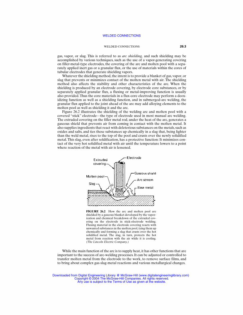
gas, vapor, or slag. This is referred to as arc shielding, and such shielding may beaccomplished by various techniques, such as the use of a vapor-generating coveringon filler-metal-type electrodes, the covering of the arc and molten pool with a sepa-rately applied inert gas or a granular flux, or the use of materials within the cores oftubular electrodes that generate shielding vapors.
Whatever the shielding method, the intent is to provide a blanket of gas, vapor, orslag that prevents or minimizes contact of the molten metal with air. The shieldingmethod also affects the stability and other characteristics of the arc. When theshielding is produced by an electrode covering, by electrode core substances, or byseparately applied granular flux, a fluxing or metal-improving function is usuallyalso provided. Thus the core materials in a flux-core electrode may perform a deox-idizing function as well as a shielding function, and in submerged-arc welding, thegranular flux applied to the joint ahead of the arc may add alloying elements to themolten pool as well as shielding it and the arc.
Figure 26.2 illustrates the shielding of the welding arc and molten pool with acovered “stick” electrode—the type of electrode used in most manual arc welding.The extruded covering on the filler metal rod, under the heat of the arc, generates agaseous shield that prevents air from coming in contact with the molten metal. Italso supplies ingredients that react with deleterious substances on the metals, such asoxides and salts, and ties these substances up chemically in a slag that, being lighterthan the weld metal, rises to the top of the pool and crusts over the newly solidifiedmetal. This slag, even after soldification, has a protective function: It minimizes con-tact of the very hot solidified metal with air until the temperature lowers to a pointwhere reaction of the metal with air is lessened.
While the main function of the arc is to supply heat, it has other functions that areimportant to the success of arc-welding processes. It can be adjusted or controlled totransfer molten metal from the electrode to the work, to remove surface films, andto bring about complex gas-slag-metal reactions and various metallurgical changes.
WELDED CONNECTIONS 26.3
FIGURE 26.2 How the arc and molten pool areshielded by a gaseous blanket developed by the vapor-ization and chemical breakdown of the extruded cov-ering on the electrode in stick-electrode welding.Fluxing material in the electrode covering reacts withunwanted substances in the molten pool, tying them upchemically and forming a slag that crusts over the hotsolidified metal. The slag, in turn, protects the hotmetal from reaction with the air while it is cooling.(The Lincoln Electric Company.)
WELDED CONNECTIONS
Downloaded from Digital Engineering Library @ McGraw-Hill (www.digitalengineeringlibrary.com)Copyright © 2004 The McGraw-Hill Companies. All rights reserved.
Any use is subject to the Terms of Use as given at the website.
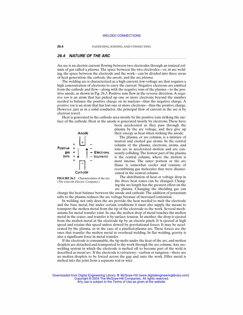
26.4 NATURE OF THE ARC
An arc is an electric current flowing between two electrodes through an ionized col-umn of gas called a plasma. The space between the two electrodes—or, in arc weld-ing, the space between the electrode and the work—can be divided into three areasof heat generation: the cathode, the anode, and the arc plasma.
The welding arc is characterized as a high-current, low-voltage arc that requires ahigh concentration of electrons to carry the current. Negative electrons are emittedfrom the cathode and flow—along with the negative ions of the plasma—to the pos-itive anode, as shown in Fig. 26.3. Positive ions flow in the reverse direction. A nega-tive ion is an atom that has picked up one or more electrons beyond the numberneeded to balance the positive charge on its nucleus—thus the negative charge. Apositive ion is an atom that has lost one or more electrons—thus the positive charge.However, just as in a solid conductor, the principal flow of current in the arc is byelectron travel.
Heat is generated in the cathode area mostly by the positive ions striking the sur-face of the cathode. Heat at the anode is generated mostly by electrons. These have
been accelerated as they pass through theplasma by the arc voltage, and they give uptheir energy as heat when striking the anode.
The plasma, or arc column, is a mixture ofneutral and excited gas atoms. In the centralcolumn of the plasma, electrons, atoms, andions are in accelerated motion and are con-stantly colliding.The hottest part of the plasmais the central column, where the motion ismost intense. The outer portion or the arcflame is somewhat cooler and consists ofrecombining gas molecules that were disasso-ciated in the central column.
The distribution of heat or voltage drop inthe three heat zones can be changed. Chang-ing the arc length has the greatest effect on thearc plasma. Changing the shielding gas can
change the heat balance between the anode and cathode. The addition of potassiumsalts to the plasma reduces the arc voltage because of increased ionization.
In welding, not only does the arc provide the heat needed to melt the electrodeand the base metal, but under certain conditions it must also supply the means totransport the molten metal from the tip of the electrode to the work. Several mech-anisms for metal transfer exist. In one, the molten drop of metal touches the moltenmetal in the crater, and transfer is by surface tension. In another, the drop is ejectedfrom the molten metal at the electrode tip by an electric pinch. It is ejected at highspeed and retains this speed unless slowed by gravitational forces. It may be accel-erated by the plasma, as in the case of a pinched-plasma arc. These forces are theones that transfer the molten metal in overhead welding. In flat welding, gravity isalso a significant force in metal transfer.
If the electrode is consumable, the tip melts under the heat of the arc, and moltendroplets are detached and transported to the work through the arc column.Any arc-welding system in which the electrode is melted off to become part of the weld isdescribed as metal arc. If the electrode is refractory—carbon or tungsten—there areno molten droplets to be forced across the gap and onto the work. Filler metal ismelted into the joint from a separate rod or wire.
26.4 FASTENING, JOINING, AND CONNECTING
FIGURE 26.3 Characteristics of the arc.(The Lincoln Electric Company.)
WELDED CONNECTIONS
Downloaded from Digital Engineering Library @ McGraw-Hill (www.digitalengineeringlibrary.com)Copyright © 2004 The McGraw-Hill Companies. All rights reserved.
Any use is subject to the Terms of Use as given at the website.
More of the heat developed by the arc ends up in the weld pool with consumableelectrodes than with nonconsumable electrodes, with the result that higher thermalefficiencies and narrower heat-affected zones are obtained.Typical thermal efficien-cies for metal-arc welding are in the 75 to 80 percent range; for welding with non-consumable electrodes, efficiencies are 50 to 60 percent.
Since there must be an ionized path to conduct electricity across a gap, the mereswitching on of the welding current with a cold electrode poised over the work willnot start the arc. The arc must first be ignited. This is accomplished either by supply-ing an initial voltage high enough to cause a discharge or by touching the electrodeto the work and then withdrawing it as the contact area becomes heated. High-frequency spark discharges are frequently used for igniting gas-shielded arcs, but themost common method of striking an arc is the touch-and-withdraw method.
Arc welding may be done with either alternating or direct current and with theelectrode either positive or negative. The choice of current and polarity depends onthe process, the type of electrode, the arc atmosphere, and the metal being welded.Whatever the current, it must be controlled to satisfy the variables—amperage andvoltage—which are specified by the welding procedures.
26.5 OVERCOMING CURRENT LIMITATIONS
The objective in commercial welding is to get the job done as fast as possible so as tolessen the time costs of skilled workers. One way to speed the welding process is toraise the current—use a higher amperage—since the faster electrical energy can beinduced in the weld joint, the faster will be the welding rate.
With manual stick-electrode welding, however, there is a practical limit to thecurrent. The covered electrodes are from 9 to 18 in long, and if the current is raisedtoo high, electrical resistance heating within the unused length of electrode willbecome so great that the covering overheats and “breaks down”—the coveringingredients react with each other or oxidize and do not function properly at the arc.Also, the hot core wire increases the melt-off rate and the arc characteristics change.The mechanics of stick-electrode welding are such that electric contact with the elec-trode cannot be made immediately above the arc—a technique that would circum-vent much of the resistance heating.
Not until semiautomatic guns and automatic welding heads (which are fed bycontinuous electrode wires) were developed was there a way of solving the resis-tance-heating problem and thus making feasible the use of high currents to speedthe welding process. In such guns and heads, electric contact with the electrode ismade close to the arc. The length between the tip of the electrode and the point ofelectric contact is then inadequate for enough resistance heating to take place tooverheat the electrode in advance of the arc, even with currents two or three timesthose usable with stick-electrode welding.
This solving of the point-of-contact problem and circumventing of the effects ofresistance heating in the electrode constituted a breakthrough that substantiallylowered welding costs and increased the use of arc welding in industrial metalsjoining. In fact, through the ingenuity of welding equipment manufacturers, theresistance-heating effect has been put to work constructively in a techniqueknown as long-stickout welding. Here, the length of electrode between the point ofelectric contact in the welding gun or head and the arc is adjusted so that resis-tance heating almost—but not quite—overheats the protruding electrode. Thuswhen a point on the electrode reaches the arc, the metal at that point is about
WELDED CONNECTIONS 26.5
WELDED CONNECTIONS
Downloaded from Digital Engineering Library @ McGraw-Hill (www.digitalengineeringlibrary.com)Copyright © 2004 The McGraw-Hill Companies. All rights reserved.
Any use is subject to the Terms of Use as given at the website.
ready to melt and less arc heat is required to melt it. Because of this, still higherwelding speeds are possible.
26.6 COMMERCIAL ARC-WELDING PROCESSES
26.6.1 Shielded Metal-Arc Welding
The shielded metal-arc process—commonly called stick-electrode welding or manualwelding—is the most widely used of the various arc-welding processes. It is charac-terized by application versatility and flexibility and relative simplicity in equipment.It is the process used by the small welding shop, by the home mechanic, and by thefarmer for repair of equipment; it is also a process having extensive application inindustrial fabrication, structural steel erection, weldment manufacture, and othercommercial metals joining. Arc welding, to persons only casually acquainted withwelding, usually means shielded metal-arc welding.
With this process, an electric arc is struck between the electrically groundedwork and a 9- to 18-in length of covered metal rod—the electrode. The electrodeis clamped in an electrode holder, which is joined by a cable to the power source.The welder grips the insulated handle of the electrode holder and maneuvers thetip of the electrode with respect to the weld joint. When the welder touches the tipof the electrode against the work and then withdraws it to establish the arc, thewelding circuit is completed. The heat of the arc melts base metal in the imme-diate area, the electrode’s metal core, and any metal particles that may be in the electrode’s covering. It also melts, vaporizes, or breaks down chemically nonmetallic substances incorporated in the covering for arc-shielding, metal-protection, or metal-conditioning purposes. The mixing of molten base metal andfiller metal from the electrode provides the coalescence required to effect joining(see Fig. 26.2).
As welding progresses, the covered rod becomes shorter and shorter. Finally, thewelding must be stopped to remove the stub and replace it with a new electrode.Thisperiodic changing of electrodes is one of the major disadvantages of the process inproduction welding. It decreases the operating factor, or the percent of the welder’stime spent in the actual laying of weld beads.
Another disadvantage of shielded metal-arc welding is the limitation placed onthe current that can be used. High amperages, such as those used with semiauto-matic guns or automatic welding heads, are impractical because of the long (andvarying) length of electrode between the arc and the point of electric contact inthe jaws of the electrode holder. The welding current is limited by the resistanceheating of the electrode. The electrode temperature must not exceed the break-down temperature of the covering. If the temperature is too high, the coveringchemicals react with each other or with air and therefore do not function properlyat the arc.
The versatility of the process—plus the simplicity of equipment—is viewed bymany users whose work would permit some degree of mechanized welding as over-riding its inherent disadvantages. This point of view was formerly well taken, butnow that semiautomatic self-shielded flux-cored arc welding has been developed toa similar (or even superior) degree of versatility and flexibility, there is less justifica-tion for adhering to stick-electrode welding in steel fabrication and erection wher-ever substantial amounts of weld metals must be placed.
26.6 FASTENING, JOINING, AND CONNECTING
WELDED CONNECTIONS
Downloaded from Digital Engineering Library @ McGraw-Hill (www.digitalengineeringlibrary.com)Copyright © 2004 The McGraw-Hill Companies. All rights reserved.
Any use is subject to the Terms of Use as given at the website.
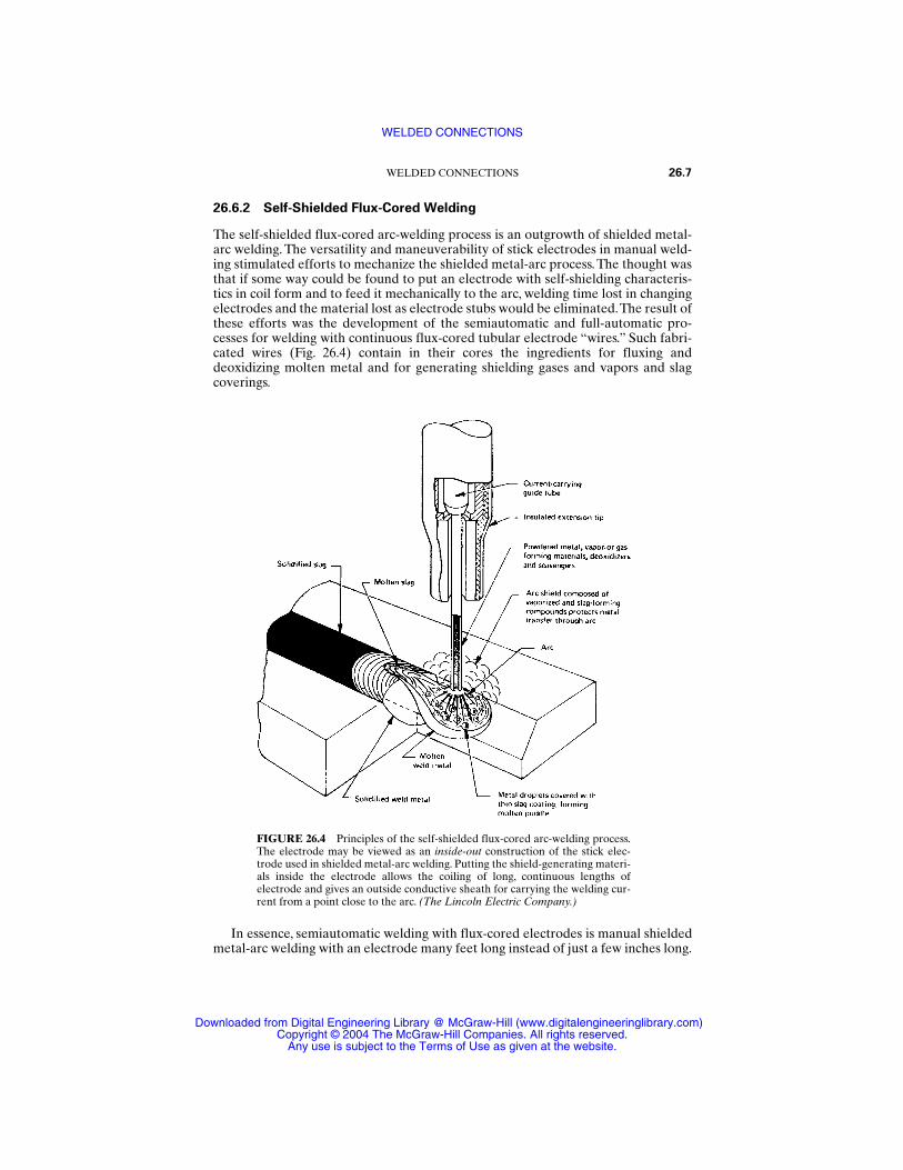
26.6.2 Self-Shielded Flux-Cored Welding
The self-shielded flux-cored arc-welding process is an outgrowth of shielded metal-arc welding. The versatility and maneuverability of stick electrodes in manual weld-ing stimulated efforts to mechanize the shielded metal-arc process. The thought wasthat if some way could be found to put an electrode with self-shielding characteris-tics in coil form and to feed it mechanically to the arc, welding time lost in changingelectrodes and the material lost as electrode stubs would be eliminated.The result ofthese efforts was the development of the semiautomatic and full-automatic pro-cesses for welding with continuous flux-cored tubular electrode “wires.” Such fabri-cated wires (Fig. 26.4) contain in their cores the ingredients for fluxing anddeoxidizing molten metal and for generating shielding gases and vapors and slagcoverings.
In essence, semiautomatic welding with flux-cored electrodes is manual shieldedmetal-arc welding with an electrode many feet long instead of just a few inches long.
WELDED CONNECTIONS 26.7
FIGURE 26.4 Principles of the self-shielded flux-cored arc-welding process.The electrode may be viewed as an inside-out construction of the stick elec-trode used in shielded metal-arc welding. Putting the shield-generating materi-als inside the electrode allows the coiling of long, continuous lengths ofelectrode and gives an outside conductive sheath for carrying the welding cur-rent from a point close to the arc. (The Lincoln Electric Company.)
WELDED CONNECTIONS
Downloaded from Digital Engineering Library @ McGraw-Hill (www.digitalengineeringlibrary.com)Copyright © 2004 The McGraw-Hill Companies. All rights reserved.
Any use is subject to the Terms of Use as given at the website.
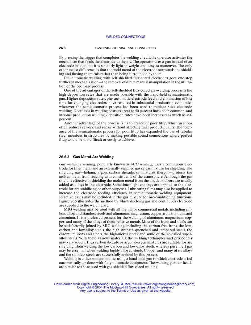
By pressing the trigger that completes the welding circuit, the operator activates themechanism that feeds the electrode to the arc.The operator uses a gun instead of anelectrode holder, but it is similarly light in weight and easy to maneuver. The onlyother major difference is that the weld metal of the electrode surrounds the shield-ing and fluxing chemicals rather than being surrounded by them.
Full-automatic welding with self-shielded flux-cored electrodes goes one stepfurther in mechanization—the removal of direct manual manipulation in the utiliza-tion of the open-arc process.
One of the advantages of the self-shielded flux-cored arc-welding process is thehigh deposition rates that are made possible with the hand-held semiautomaticgun. Higher deposition rates, plus automatic electrode feed and elimination of losttime for changing electrodes, have resulted in substantial production economieswherever the semiautomatic process has been used to replace stick-electrodewelding. Decreases in welding costs as great as 50 percent have been common, andin some production welding, deposition rates have been increased as much as 400percent.
Another advantage of the process is its tolerance of poor fitup, which in shopsoften reduces rework and repair without affecting final product quality. The toler-ance of the semiautomatic process for poor fitup has expanded the use of tubularsteel members in structures by making possible sound connections where perfectfitup would be too difficult or costly to achieve.
26.6.3 Gas Metal-Arc Welding
Gas metal-arc welding, popularly known as MIG welding, uses a continuous elec-trode for filler metal and an externally supplied gas or gas mixture for shielding.Theshielding gas—helium, argon, carbon dioxide, or mixtures thereof—protects themolten metal from reacting with constituents of the atmosphere. Although the gasshield is effective in shielding the molten metal from the air, deoxidizers are usuallyadded as alloys in the electrode. Sometimes light coatings are applied to the elec-trode for arc stabilizing or other purposes. Lubricating films may also be applied toincrease the electrode feeding efficiency in semiautomatic welding equipment.Reactive gases may be included in the gas mixture for arc-conditioning functions.Figure 26.5 illustrates the method by which shielding gas and continuous electrodeare supplied to the welding arc.
MIG welding may be used with all the major commercial metals, including car-bon, alloy, and stainless steels and aluminum, magnesium, copper, iron, titanium, andzirconium. It is a preferred process for the welding of aluminum, magnesium, cop-per, and many of the alloys of these reactive metals. Most of the irons and steels canbe satisfactorily joined by MIG welding, including the carbon-free irons, the low-carbon and low-alloy steels, the high-strength quenched and tempered steels, thechromium irons and steels, the high-nickel steels, and some of the so-called super-alloy steels. With these various materials, the welding techniques and proceduresmay vary widely. Thus carbon dioxide or argon-oxygen mixtures are suitable for arcshielding when welding the low-carbon and low-alloy steels, whereas pure inert gasmay be essential when welding highly alloyed steels. Copper and many of its alloysand the stainless steels are successfully welded by this process.
Welding is either semiautomatic, using a hand-held gun to which electrode is fedautomatically, or done with fully automatic equipment. The welding guns or headsare similar to those used with gas-shielded flux-cored welding.
26.8 FASTENING, JOINING, AND CONNECTING
WELDED CONNECTIONS
Downloaded from Digital Engineering Library @ McGraw-Hill (www.digitalengineeringlibrary.com)Copyright © 2004 The McGraw-Hill Companies. All rights reserved.
Any use is subject to the Terms of Use as given at the website.
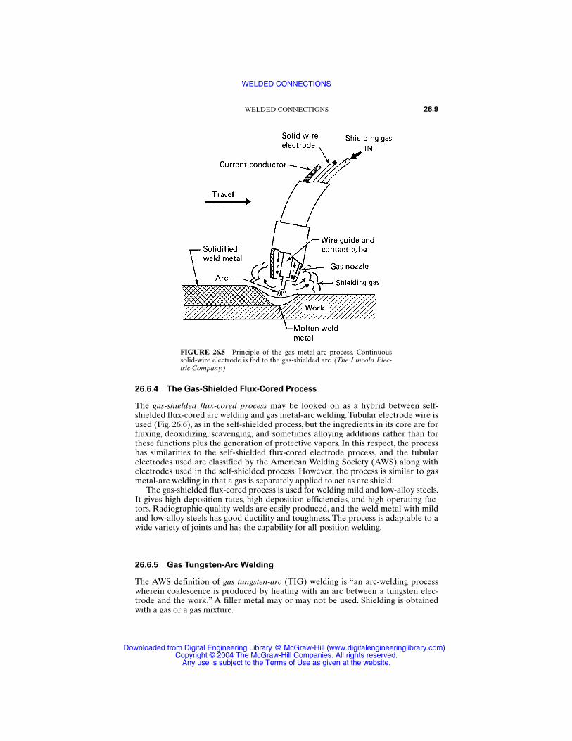
26.6.4 The Gas-Shielded Flux-Cored Process
The gas-shielded flux-cored process may be looked on as a hybrid between self-shielded flux-cored arc welding and gas metal-arc welding. Tubular electrode wire isused (Fig. 26.6), as in the self-shielded process, but the ingredients in its core are forfluxing, deoxidizing, scavenging, and sometimes alloying additions rather than forthese functions plus the generation of protective vapors. In this respect, the processhas similarities to the self-shielded flux-cored electrode process, and the tubularelectrodes used are classified by the American Welding Society (AWS) along withelectrodes used in the self-shielded process. However, the process is similar to gasmetal-arc welding in that a gas is separately applied to act as arc shield.
The gas-shielded flux-cored process is used for welding mild and low-alloy steels.It gives high deposition rates, high deposition efficiencies, and high operating fac-tors. Radiographic-quality welds are easily produced, and the weld metal with mildand low-alloy steels has good ductility and toughness. The process is adaptable to awide variety of joints and has the capability for all-position welding.
26.6.5 Gas Tungsten-Arc Welding
The AWS definition of gas tungsten-arc (TIG) welding is “an arc-welding processwherein coalescence is produced by heating with an arc between a tungsten elec-trode and the work.” A filler metal may or may not be used. Shielding is obtainedwith a gas or a gas mixture.
WELDED CONNECTIONS 26.9
FIGURE 26.5 Principle of the gas metal-arc process. Continuoussolid-wire electrode is fed to the gas-shielded arc. (The Lincoln Elec-tric Company.)
WELDED CONNECTIONS
Downloaded from Digital Engineering Library @ McGraw-Hill (www.digitalengineeringlibrary.com)Copyright © 2004 The McGraw-Hill Companies. All rights reserved.
Any use is subject to the Terms of Use as given at the website.
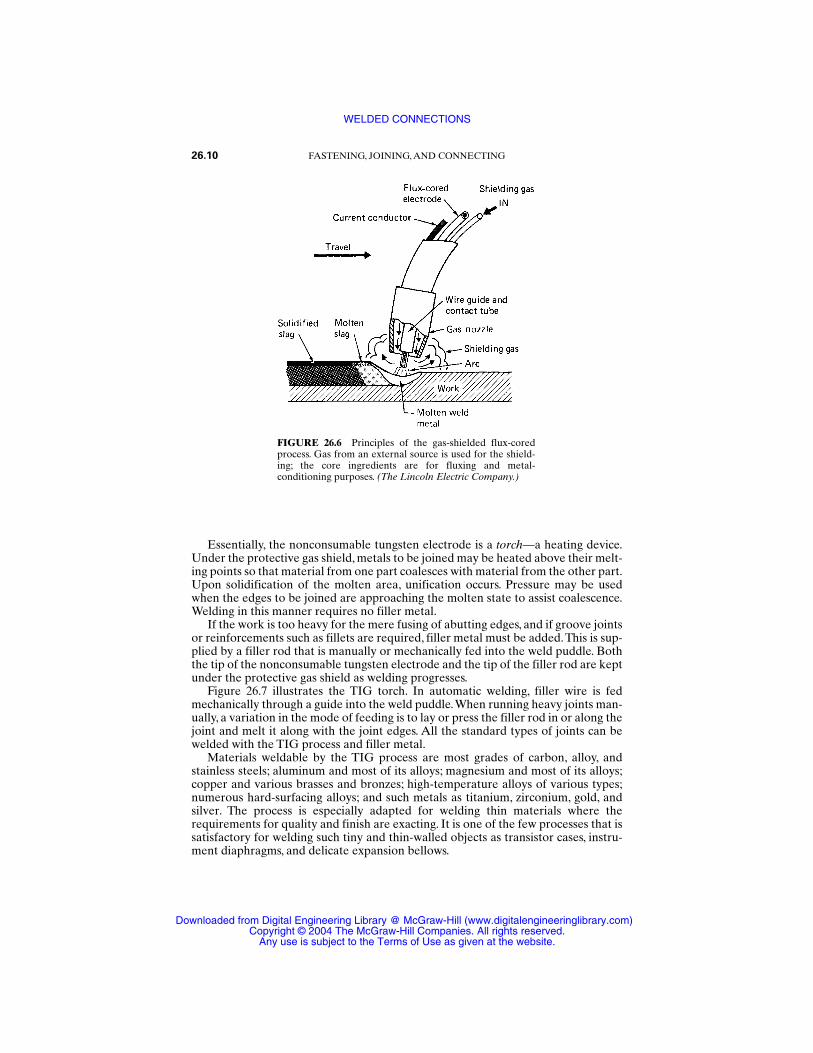
Essentially, the nonconsumable tungsten electrode is a torch—a heating device.Under the protective gas shield, metals to be joined may be heated above their melt-ing points so that material from one part coalesces with material from the other part.Upon solidification of the molten area, unification occurs. Pressure may be usedwhen the edges to be joined are approaching the molten state to assist coalescence.Welding in this manner requires no filler metal.
If the work is too heavy for the mere fusing of abutting edges, and if groove jointsor reinforcements such as fillets are required, filler metal must be added.This is sup-plied by a filler rod that is manually or mechanically fed into the weld puddle. Boththe tip of the nonconsumable tungsten electrode and the tip of the filler rod are keptunder the protective gas shield as welding progresses.
Figure 26.7 illustrates the TIG torch. In automatic welding, filler wire is fedmechanically through a guide into the weld puddle.When running heavy joints man-ually, a variation in the mode of feeding is to lay or press the filler rod in or along thejoint and melt it along with the joint edges. All the standard types of joints can bewelded with the TIG process and filler metal.
Materials weldable by the TIG process are most grades of carbon, alloy, andstainless steels; aluminum and most of its alloys; magnesium and most of its alloys;copper and various brasses and bronzes; high-temperature alloys of various types;numerous hard-surfacing alloys; and such metals as titanium, zirconium, gold, andsilver. The process is especially adapted for welding thin materials where therequirements for quality and finish are exacting. It is one of the few processes that issatisfactory for welding such tiny and thin-walled objects as transistor cases, instru-ment diaphragms, and delicate expansion bellows.
26.10 FASTENING, JOINING, AND CONNECTING
FIGURE 26.6 Principles of the gas-shielded flux-coredprocess. Gas from an external source is used for the shield-ing; the core ingredients are for fluxing and metal-conditioning purposes. (The Lincoln Electric Company.)
WELDED CONNECTIONS
Downloaded from Digital Engineering Library @ McGraw-Hill (www.digitalengineeringlibrary.com)Copyright © 2004 The McGraw-Hill Companies. All rights reserved.
Any use is subject to the Terms of Use as given at the website.
26.6.6 Submerged-Arc Welding
Submerged-arc welding differs from other arc-welding processes in that a blanket offusible granular material—commonly called flux—is used for shielding the arc andthe molten metal.The arc is struck between the workpiece and a bare wire electrode,the tip of which is submerged in the flux. Since the arc is completely covered by theflux, it is not visible, and the weld is run without the flash, spatter, and sparks thatcharacterize the open-arc process. The nature of the flux is such that very littlesmoke or visible fumes are developed.
The process is either semiautomatic or fully automatic, and the electrode is fedmechanically to the welding gun, head, or heads. In semiautomatic welding, thewelder moves the gun, usually equipped with a flux-feeding device, along the joint.Flux feed may be by gravity flow through a nozzle concentric with the electrodefrom a small hopper atop the gun, or it may be through a concentric nozzle tube con-nected to an air-pressurized flux tank. Flux may also be applied in advance of thewelding operation or ahead of the arc from a hopper run along the joint. In fullyautomatic submerged-arc welding, flux is fed continuously to the joint ahead of orconcentric with the arc, and fully automatic installations are commonly equippedwith vacuum systems to pick up the unfused flux left by the welding head or headsfor cleaning and reuse.
During welding, the heat of the arc melts some of the flux along with the tip of theelectrode, as illustrated in Fig. 26.8.The tip of the electrode and the welding zone arealways surrounded and shielded by molten flux, surmounted by a layer of unfusedflux. The electrode is held a short distance above the workpiece. As the electrodeprogresses along the joint, the lighter molten flux rises above the molten metal in theform of a slag. The weld metal, having a higher melting (freezing) point, solidifies
WELDED CONNECTIONS 26.11
FIGURE 26.7 Principles of the gas tungsten-arc process. If fillermetal is required, it is fed into the pool from a separate filler rod.(The Lincoln Electric Company.)
WELDED CONNECTIONS
Downloaded from Digital Engineering Library @ McGraw-Hill (www.digitalengineeringlibrary.com)Copyright © 2004 The McGraw-Hill Companies. All rights reserved.
Any use is subject to the Terms of Use as given at the website.
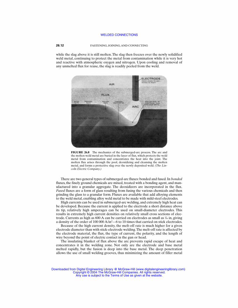
while the slag above it is still molten. The slag then freezes over the newly solidifiedweld metal, continuing to protect the metal from contamination while it is very hotand reactive with atmospheric oxygen and nitrogen. Upon cooling and removal ofany unmelted flux for reuse, the slag is readily peeled from the weld.
There are two general types of submerged-arc fluxes: bonded and fused. In bondedfluxes, the finely ground chemicals are mixed, treated with a bonding agent, and man-ufactured into a granular aggregate. The deoxidizers are incorporated in the flux.Fused fluxes are a form of glass resulting from fusing the various chemicals and thengrinding the glass to a granular form. Fluxes are available that add alloying elementsto the weld metal, enabling alloy weld metal to be made with mild-steel electrodes.
High currents can be used in submerged-arc welding, and extremely high heat canbe developed. Because the current is applied to the electrode a short distance aboveits tip, relatively high amperages can be used on small-diameter electrodes. Thisresults in extremely high current densities on relatively small cross sections of elec-trode. Currents as high as 600 A can be carried on electrodes as small as 5⁄64 in, givinga density of the order of 100 000 A/in2—6 to 10 times that carried on stick electrodes.
Because of the high current density, the melt-off rate is much higher for a givenelectrode diameter than with stick-electrode welding.The melt-off rate is affected bythe electrode material, the flux, the type of current, the polarity, and the length ofwire beyond the point of electric contact in the gun or head.
The insulating blanket of flux above the arc prevents rapid escape of heat andconcentrates it in the welding zone. Not only are the electrode and base metalmelted rapidly, but the fusion is deep into the base metal. The deep penetrationallows the use of small welding grooves, thus minimizing the amount of filler metal
26.12 FASTENING, JOINING, AND CONNECTING
FIGURE 26.8 The mechanics of the submerged-arc process. The arc andthe molten weld metal are buried in the layer of flux, which protects the weldmetal from contamination and concentrates the heat into the joint. Themolten flux arises through the pool, deoxidizing and cleansing the moltenmetal, and forms a protective slag over the newly deposited weld. (The Lin-coln Electric Company.)
WELDED CONNECTIONS
Downloaded from Digital Engineering Library @ McGraw-Hill (www.digitalengineeringlibrary.com)Copyright © 2004 The McGraw-Hill Companies. All rights reserved.
Any use is subject to the Terms of Use as given at the website.
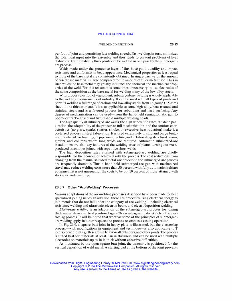
per foot of joint and permitting fast welding speeds. Fast welding, in turn, minimizesthe total heat input into the assembly and thus tends to prevent problems of heatdistortion. Even relatively thick joints can be welded in one pass by the submerged-arc process.
Welds made under the protective layer of flux have good ductility and impactresistance and uniformity in bead appearance. Mechanical properties at least equalto those of the base metal are consistently obtained. In single-pass welds, the amountof fused base material is large compared to the amount of filler metal used. Thus insuch welds the base metal may greatly influence the chemical and mechanical prop-erties of the weld. For this reason, it is sometimes unnecessary to use electrodes ofthe same composition as the base metal for welding many of the low-alloy steels.
With proper selection of equipment, submerged-arc welding is widely applicableto the welding requirements of industry. It can be used with all types of joints andpermits welding a full range of carbon and low-alloy steels, from 16-gauge (1.5-mm)sheet to the thickest plate. It is also applicable to some high-alloy, heat-treated, andstainless steels and is a favored process for rebuilding and hard surfacing. Anydegree of mechanization can be used—from the hand-held semiautomatic gun toboom- or track-carried and fixture-held multiple welding heads.
The high quality of submerged-arc welds, the high deposition rates, the deep pen-etration, the adaptability of the process to full mechanization, and the comfort char-acteristics (no glare, sparks, spatter, smoke, or excessive heat radiation) make it apreferred process in steel fabrication. It is used extensively in ship and barge build-ing, in railroad car building, in pipe manufacture, and in fabricating structural beams,girders, and columns where long welds are required. Automatic submerged-arcinstallations are also key features of the welding areas of plants turning out mass-produced assemblies joined with repetitive short welds.
The high deposition rates attained with submerged-arc welding are chieflyresponsible for the economies achieved with the process. The cost reductions fromchanging from the manual shielded metal-arc process to the submerged-arc processare frequently dramatic. Thus a hand-held submerged-arc gun with mechanizedtravel may reduce welding costs more than 50 percent; with fully automatic multiarcequipment, it is not unusual for the costs to be but 10 percent of those attained withstick-electrode welding.
26.6.7 Other “Arc-Welding” Processes
Various adaptations of the arc-welding processes described have been made to meetspecialized joining needs. In addition, there are processes using electrical energy tojoin metals that do not fall under the category of arc welding—including electricalresistance welding and ultrasonic, electron beam, and electrodeposition welding.
Electroslag welding is an adaptation of the submerged-arc process for joiningthick materials in a vertical position. Figure 26.9 is a diagrammatic sketch of the elec-troslag process. It will be noted that whereas some of the principles of submerged-arc welding apply, in other respects the process resembles a casting operation.
In Fig. 26.9, a square butt joint in heavy plate is illustrated, but the electroslagprocess—with modifications in equipment and technique—is also applicable to Tjoints, corner joints, girth seams in heavy-wall cylinders, and other joints.The processis suited best for materials at least 1 in in thickness and can be used with multipleelectrodes on materials up to 10 in thick without excessive difficulties.
As illustrated by the open square butt joint, the assembly is positioned for thevertical deposition of weld metal. A starting pad at the bottom of the joint prevents
WELDED CONNECTIONS 26.13
WELDED CONNECTIONS
Downloaded from Digital Engineering Library @ McGraw-Hill (www.digitalengineeringlibrary.com)Copyright © 2004 The McGraw-Hill Companies. All rights reserved.
Any use is subject to the Terms of Use as given at the website.
the fall-out of the initially deposited weld metal and, since it is penetrated, ensures afull weld at this point. Welding is started at the bottom and progresses upward.Water-cooled dams, which may be looked on as molds, are placed on each side of thejoint. These dams are moved upward as the weld-metal deposition progresses. Thejoint is filled in one pass—a single upward progression—of one or more consumableelectrodes.The electrode or electrodes may be oscillated across the joint if the widthof the joint makes this desirable.
At the start of the operation, a layer of flux is placed in the bottom of the jointand an arc is struck between the electrode (or electrodes) and the work. The arcmelts the slag, forming a molten layer, which subsequently acts as an electrolyticheating medium. The arc is then quenched or shorted-out by this molten conductivelayer. Heat for melting the electrode and the base metal subsequently results fromthe electrical resistance heating of the electrode section extending from the contacttube and from the resistance heating within the molten slag layer. As the electrode(or electrodes) is consumed, the welding head (or heads) and the cooling dams moveupward.
In conventional practice, the weld deposit usually contains about one-thirdmelted base metal and two-thirds electrode metal—which means that the base metalsubstantially contributes to the chemical composition of the weld metal. Flux con-sumption is low, since the molten flux and the unmelted flux above it “ride” abovethe progressing weld.
The flux used has a degree of electrical conductivity and low viscosity in themolten condition and a high vaporization temperature. The consumable electrodesmay be either solid wire or tubular wire filled with metal powders.Alloying elementsmay be incorporated into the weld by each of these electrodes.
26.14 FASTENING, JOINING, AND CONNECTING
FIGURE 26.9 Schematic sketch of electroslag welding: (1) elec-trode guide tube, (2) electrode, (3) water-cooled copper shoes, (4)finished weld, (5) base metal, (6) molten slag, (7) molten weld metal,and (8) solidified weld metal. (The Lincoln Electric Company.)
WELDED CONNECTIONS
Downloaded from Digital Engineering Library @ McGraw-Hill (www.digitalengineeringlibrary.com)Copyright © 2004 The McGraw-Hill Companies. All rights reserved.
Any use is subject to the Terms of Use as given at the website.
Weld quality with the electroslag process is generally excellent, because of theprotective action of the heavy slag layer. Sometimes, however, the copper dams areprovided with orifices just above the slag layer through which a protective gas—argon or carbon dioxide—is introduced to flush out the air above the weld and thusgive additional assurance against oxidation. Such provisions are sometimes consid-ered worthwhile when welding highly alloyed steels or steels that contain easily oxi-dized elements.
Electrogas welding is very similar to electroslag welding in that the equipment issimilar and the joint is in the vertical position. As the name implies, the shielding isby carbon dioxide or an inert gas. A thin layer of slag, supplied by the flux-coredelectrode, covers the molten metal, and the heat is supplied by an arc rather than byresistance heating, as in the electroslag process.
A disadvantage of the process is that it requires an external source of shieldinggas. However, one advantage is that if the welding is stopped, the electrogas processcan be started again with less difficulty than the electroslag process.
Stud arc welding is a variation of the shielded metal-arc process that is widelyused for attaching studs, screws, pins, and similar fasteners to a large workpiece. Thestud (or small part) itself—often plus a ceramic ferrule at its tip—is the arc-weldingelectrode during the brief period of time required for studding.
In operation, the stud is held in a portable pistol-shaped tool called a stud gunand positioned by the operator over the spot where it is to be weld-attached. At apress of the trigger, current flows through the stud, which is lifted slightly, creating anarc. After a very short arcing period, the stud is then plunged down into the moltenpool created on the base plate, the gun is withdrawn from it, and the ceramic fer-rule—if one has been used—is removed. The timing is controlled automatically, andthe stud is welded onto the workpiece in less than a second.The fundamentals of theprocess are illustrated in Fig. 26.10.
Studs are of many shapes. All may be weld-attached with portable equipment.The stud may be used with a ceramic arc-shielding ferrule, as shown in Fig. 26.10,which prevents air infiltration and also acts as a dam to retain the molten metal, orit may have a granular flux, flux coating, or solid flux affixed to the welding end, asillustrated in Fig. 26.11. The flux may include any of the agents found in a regularelectrode covering; most important to stud welding is a deoxidizer to guard againstporosity.
Plasma-arc (or plasma-torch) welding is one of the newer welding processeswhich is used industrially, frequently as a substitute for the gas tungsten-arc process.In some applications, it offers greater welding speeds, better weld quality, and lesssensitivity to process variables than the conventional processes it replaces. With theplasma torch, temperatures as high as 60 000°F are developed, and theoretically,temperatures as high as 200 000°F are possible.
The heat in plasma-arc welding originates in an arc, but this arc is not diffused asis an ordinary welding arc. Instead, it is constricted by being forced through a rela-tively small orifice. The orifice, or plasma gas, may be supplemented by an auxiliarysource of shielding gas.
Orifice gas refers to the gas that is directed into the torch to surround the elec-trode. It becomes ionized in the arc to form the plasma and emerges from the orificein the torch nozzle as a plasma jet. If a shielding gas is used, it is directed onto theworkpiece from an outer shielding ring.
The workpiece may or may not be part of the electric circuit. In the transferred-arc system, the workpiece is a part of the circuit, as in other arc-welding processes.The arc transfers from the electrode through the orifice to the work. In the non-transferred system, the constricting nozzle surrounding the electrode acts as an elec-
WELDED CONNECTIONS 26.15
WELDED CONNECTIONS
Downloaded from Digital Engineering Library @ McGraw-Hill (www.digitalengineeringlibrary.com)Copyright © 2004 The McGraw-Hill Companies. All rights reserved.
Any use is subject to the Terms of Use as given at the website.
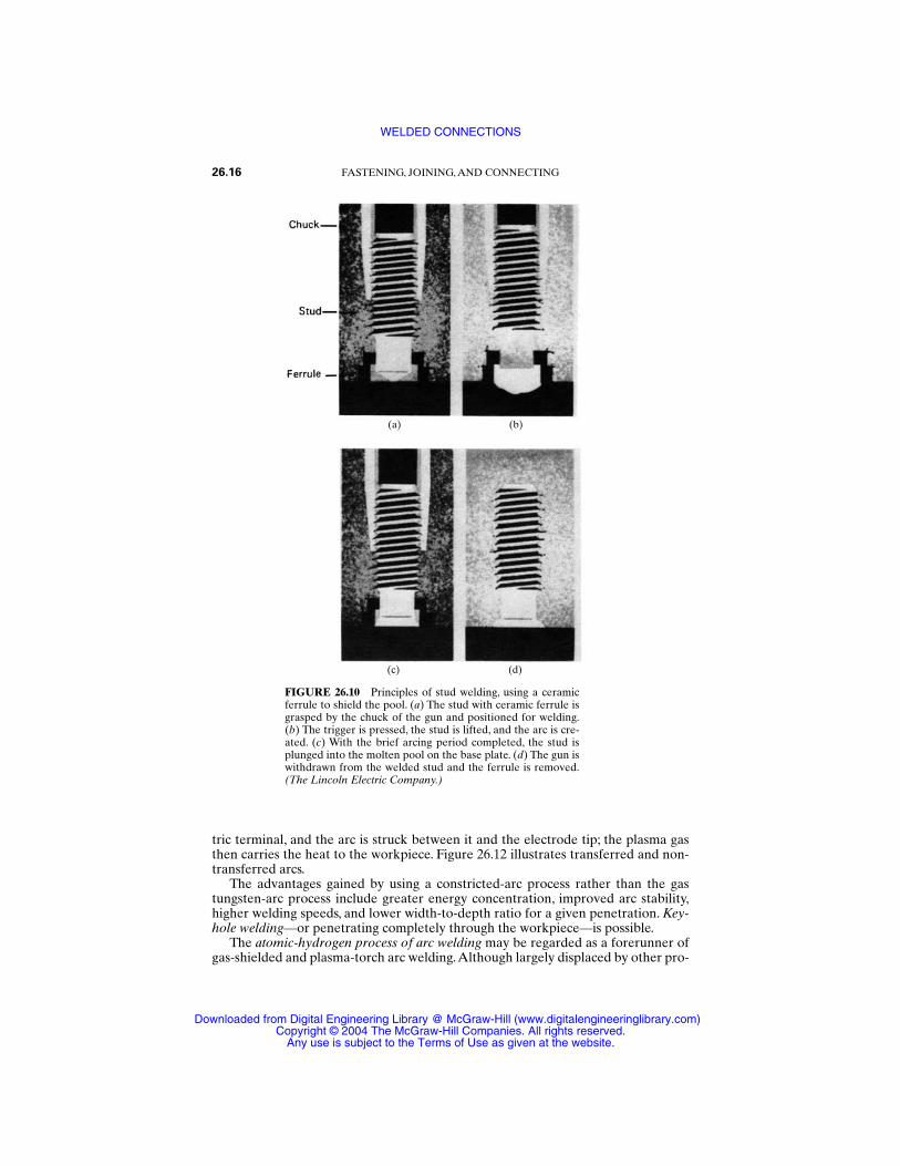
tric terminal, and the arc is struck between it and the electrode tip; the plasma gasthen carries the heat to the workpiece. Figure 26.12 illustrates transferred and non-transferred arcs.
The advantages gained by using a constricted-arc process rather than the gastungsten-arc process include greater energy concentration, improved arc stability,higher welding speeds, and lower width-to-depth ratio for a given penetration. Key-hole welding—or penetrating completely through the workpiece—is possible.
The atomic-hydrogen process of arc welding may be regarded as a forerunner ofgas-shielded and plasma-torch arc welding.Although largely displaced by other pro-
26.16 FASTENING, JOINING, AND CONNECTING
FIGURE 26.10 Principles of stud welding, using a ceramicferrule to shield the pool. (a) The stud with ceramic ferrule isgrasped by the chuck of the gun and positioned for welding.(b) The trigger is pressed, the stud is lifted, and the arc is cre-ated. (c) With the brief arcing period completed, the stud isplunged into the molten pool on the base plate. (d) The gun iswithdrawn from the welded stud and the ferrule is removed.(The Lincoln Electric Company.)
(a) (b)
(c) (d)
WELDED CONNECTIONS
Downloaded from Digital Engineering Library @ McGraw-Hill (www.digitalengineeringlibrary.com)Copyright © 2004 The McGraw-Hill Companies. All rights reserved.
Any use is subject to the Terms of Use as given at the website.
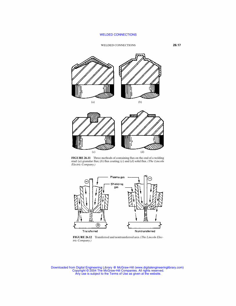
WELDED CONNECTIONS 26.17
FIGURE 26.11 Three methods of containing flux on the end of a weldingstud: (a) granular flux; (b) flux coating; (c) and (d) solid flux. (The LincolnElectric Company.)
FIGURE 26.12 Transferred and nontransferred arcs. (The Lincoln Elec-tric Company.)
(c) (d)
(a) (b)
WELDED CONNECTIONS
Downloaded from Digital Engineering Library @ McGraw-Hill (www.digitalengineeringlibrary.com)Copyright © 2004 The McGraw-Hill Companies. All rights reserved.
Any use is subject to the Terms of Use as given at the website.
cesses that require less skill and are less costly, it is still preferred in some manualoperations where close control of heat input is required.
In the atomic-hydrogen process, an arc is established between two tungsten elec-trodes in a stream of hydrogen gas using alternating current.As the gas passes throughthe arc, molecular hydrogen is dissociated into atomic hydrogen under the intenseheat. When the stream of hydrogen atoms strikes the workpiece, the environmentaltemperature is then at a level where recombining into molecules is possible.As a resultof the recombining, the heat of dissociation absorbed in the arc is liberated, supplyingthe heat needed for fusing the base metal and any filler metal that may be introduced.
The atomic-hydrogen process depends on an arc, but is really a heating torch.Thearc supplies the heat through the intermediate of the molecular-dissociation, atom-recombination mechanism. The hydrogen gas, however, does more than provide themechanism for heat transfer. Before entering the arc, it acts as a shield and a coolantto keep the tungsten electrodes from overheating.At the weld puddle, the gas acts asa shield. Since hydrogen is a powerful reducing agent, any rust in the weld area isreduced to iron, and no oxide can form or exist in the hydrogen atmosphere. Weldmetal, however, can absorb hydrogen, with unfavorable metallurgical effects. For thisreason, the process gives difficulties with steels containing sulfur or selenium, sincehydrogen reacts with these elements to form hydrogen sulfide or hydrogen selenidegases. These are almost insoluble in molten metal and either bubble out of the weldpool vigorously or become entrapped in the solidifying metal, resulting in porosity.
26.7 ARC-WELDING CONSUMABLES
Arc-welding consumables are the materials used up during welding, such as elec-trodes, filler rods, fluxes, and externally applied shielding gases. With the exceptionof the gases, all the commonly used consumables are covered by AWS specifications.
Twenty specifications in the AWS A5.x series prescribed the requirements forwelding electrodes, rods, and fluxes.
26.7.1 Electrodes, Rods, and Fluxes
The first specification for mild-steel-covered electrodes, A5.1, was written in 1940.As the welding industry expanded and the number of types of electrodes for weld-ing steel increased, it became necessary to devise a system of electrode classificationto avoid confusion.The system used applies to both the mild-steel A5.1 and the low-alloy steel A5.5 specifications.
Classifications of mild and low-alloy steel electrodes are based on an E prefix anda four- or five-digit number. The first two digits (or three, in a five-digit number)indicate the minimum required tensile strength in thousands of pounds per squareinch. For example, 60 = 60 kpsi, 70 = 70 kpsi, and 100 = 100 kpsi. The next to the lastdigit indicates the welding position in which the electrode is capable of making sat-isfactory welds: 1 = all positions—flat, horizontal, vertical, and overhead; 2 = flat andhorizontal fillet welding (see Table 26.1). The last digit indicates the type of currentto be used and the type of covering on the electrode (see Table 26.2).
Originally a color identification system was developed by the National ElectricalManufacturers Association (NEMA) in conjunction with the AWS to identify theelectrode’s classification. This was a system of color markings applied in a specificrelationship on the electrode, as in Fig. 26.13a. The colors and their significance are
26.18 FASTENING, JOINING, AND CONNECTING
WELDED CONNECTIONS
Downloaded from Digital Engineering Library @ McGraw-Hill (www.digitalengineeringlibrary.com)Copyright © 2004 The McGraw-Hill Companies. All rights reserved.
Any use is subject to the Terms of Use as given at the website.

listed in Tables 26.3 and 26.4. The NEMA specification also included the choice ofimprinting the classification number on the electrode, as in Fig. 26.13b.
Starting in 1964, new and revised AWS specifications for covered electrodesrequired that the classification number be imprinted on the covering, as in Fig.26.13b. However, some electrodes can be manufactured faster than the imprintingequipment can mark them, and some sizes are too small to be legibly marked withan imprint. Although AWS specifies an imprint, the color code is accepted on elec-trodes if imprinting is not practical.
Bare mild-steel electrodes (electrode wires) for submerged-arc welding are classi-fied on the basis of chemical composition, as shown in Table 26.5. In this classifyingsystem, the letter E indicates an electrode as in the other classifying systems, but
WELDED CONNECTIONS 26.19
TABLE 26.1 AWS A5.1-69 and A5.5-69 Designations for Manual Electrodes
TABLE 26.2 AWS A5.1-69 Electrode Designations for Covered Arc-Welding Electrodes
WELDED CONNECTIONS
Downloaded from Digital Engineering Library @ McGraw-Hill (www.digitalengineeringlibrary.com)Copyright © 2004 The McGraw-Hill Companies. All rights reserved.
Any use is subject to the Terms of Use as given at the website.
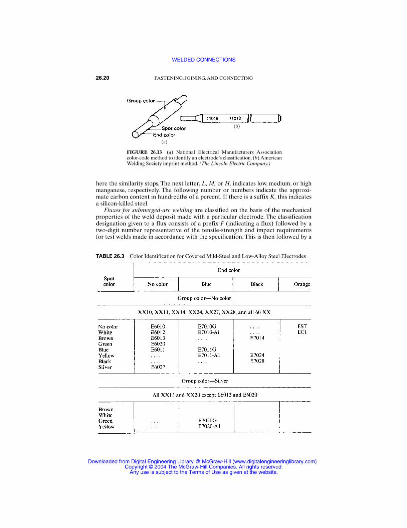
here the similarity stops. The next letter, L, M, or H, indicates low, medium, or highmanganese, respectively. The following number or numbers indicate the approxi-mate carbon content in hundredths of a percent. If there is a suffix K, this indicatesa silicon-killed steel.
Fluxes for submerged-arc welding are classified on the basis of the mechanicalproperties of the weld deposit made with a particular electrode. The classificationdesignation given to a flux consists of a prefix F (indicating a flux) followed by atwo-digit number representative of the tensile-strength and impact requirementsfor test welds made in accordance with the specification. This is then followed by a
26.20 FASTENING, JOINING, AND CONNECTING
FIGURE 26.13 (a) National Electrical Manufacturers Associationcolor-code method to identify an electrode’s classification. (b) AmericanWelding Society imprint method. (The Lincoln Electric Company.)
TABLE 26.3 Color Identification for Covered Mild-Steel and Low-Alloy Steel Electrodes
(b)
(a)
WELDED CONNECTIONS
Downloaded from Digital Engineering Library @ McGraw-Hill (www.digitalengineeringlibrary.com)Copyright © 2004 The McGraw-Hill Companies. All rights reserved.
Any use is subject to the Terms of Use as given at the website.
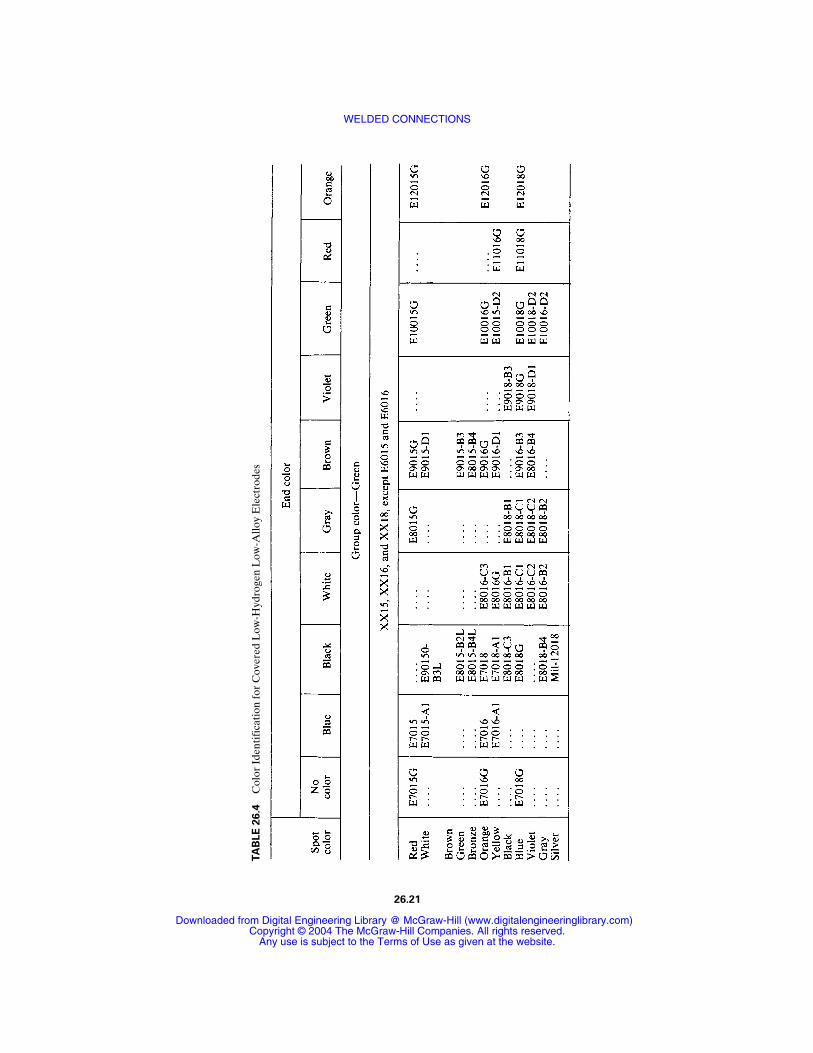
TA
BLE
26.4
Col
or I
dent
ific
atio
n fo
r C
over
ed L
ow-H
ydro
gen
Low
-Allo
y E
lect
rode
s
26.21
WELDED CONNECTIONS
Downloaded from Digital Engineering Library @ McGraw-Hill (www.digitalengineeringlibrary.com)Copyright © 2004 The McGraw-Hill Companies. All rights reserved.
Any use is subject to the Terms of Use as given at the website.
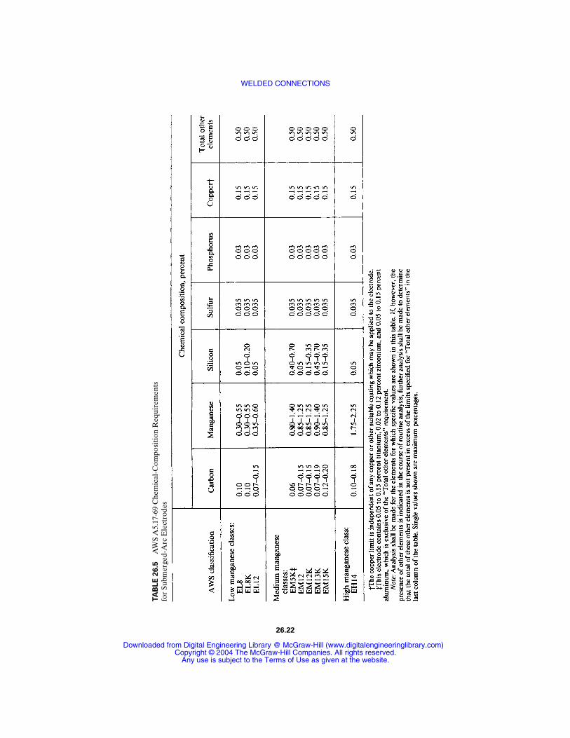
TA
BLE
26.5
AW
S A
5.17
-69
Che
mic
al-C
ompo
siti
on R
equi
rem
ents
fo
r Su
bmer
ged-
Arc
Ele
ctro
des
26.22
WELDED CONNECTIONS
Downloaded from Digital Engineering Library @ McGraw-Hill (www.digitalengineeringlibrary.com)Copyright © 2004 The McGraw-Hill Companies. All rights reserved.
Any use is subject to the Terms of Use as given at the website.
set of letters and numbers corresponding to the classification of the electrode usedwith the flux.
Gas-shielded flux-cored electrodes are available for welding the low-alloy high-tensile steels. Self-shielded flux-cored electrodes are available for all-position weld-ing, as in building construction. Fabricators using or anticipating using the flux-coredarc-welding processes should keep in touch with the electrode manufacturers fornew or improved electrodes not included in present specifications.
Mild-steel electrodes for gas metal-arc welding of mild and low-alloy steels areclassified on the basis of their chemical compositions and the as-welded mechanicalproperties of the weld metal. Tables 26.6 and 26.7 are illustrative.
AWS specifications for electrodes also cover those used for welding the stainlesssteels, aluminum and aluminum alloys, and copper and copper alloys, as well as forweld surfacing.
Shielding gases are consumables used with the MIG and TIG welding processes.The AWS does not write specifications for gases.There are federal specifications, butthe welding industry usually relies on welding grade to describe the required purity.
The primary purpose of a shielding gas is to protect the molten weld metal fromcontamination by the oxygen and nitrogen in air.The factors, in addition to cost, thataffect the suitability of a gas include the influence of the gas on the arcing and metal-transfer characteristics during welding, weld penetration, width of fusion and surfaceshape, welding speed, and the tendency to undercut. Among the inert gases—helium, argon, neon, krypton, and xenon—the only ones plentiful enough for practi-cal use in welding are helium and argon. These gases provide satisfactory shieldingfor the more reactive metals, such as aluminum, magnesium, beryllium, columbium,tantalum, titanium, and zirconium.
Although pure inert gases protect metal at any temperature from reaction withconstituents of the air, they are not suitable for all welding applications. Controlledquantities of reactive gases mixed with inert gases improve the arc action and metal-transfer characteristics when welding steels, but such mixtures are not used for reac-tive metals.
Oxygen, nitrogen, and carbon dioxide are reactive gases. With the exception ofcarbon dioxide, these gases are not generally used alone for arc shielding. Carbondioxide can be used alone or mixed with an inert gas for welding many carbon andlow-alloy steels. Oxygen is used in small quantities with one of the inert gases—usually argon. Nitrogen is occasionally used alone, but it is usually mixed with argonas a shielding gas to weld copper. The most extensive use of nitrogen is in Europe,where helium is relatively unavailable.
26.8 DESIGN OF WELDED JOINTS
While designers need some basic knowledge of welding processes, equipment, mate-rials, and techniques, their main interest is in how to transfer forces through weldedjoints most effectively and efficiently. Proper joint design is the key to good welddesign.
The loads in a welded-steel design are transferred from one member to anotherthrough welds placed in weld joints. Both the type of joint and the type of weld arespecified by the designer.
Figure 26.14 shows the joint and weld types. Specifying a joint does not by itselfdescribe the type of weld to be used. Thus 10 types of welds are shown for making a
WELDED CONNECTIONS 26.23
WELDED CONNECTIONS
Downloaded from Digital Engineering Library @ McGraw-Hill (www.digitalengineeringlibrary.com)Copyright © 2004 The McGraw-Hill Companies. All rights reserved.
Any use is subject to the Terms of Use as given at the website.
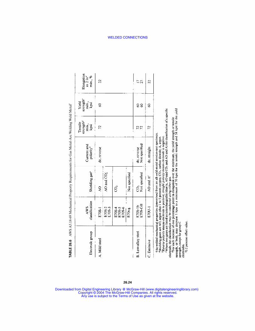
TA
BLE
26.6
AW
S A
5.18
-69
Mec
hani
cal P
rope
rty
Req
uire
men
ts fo
r G
as M
etal
-Arc
Wel
ding
Wel
d M
etal
†
26.24
WELDED CONNECTIONS
Downloaded from Digital Engineering Library @ McGraw-Hill (www.digitalengineeringlibrary.com)Copyright © 2004 The McGraw-Hill Companies. All rights reserved.
Any use is subject to the Terms of Use as given at the website.

TA
BLE
26.7
AW
S A
5.18
-69
Che
mic
al-C
ompo
siti
on R
equi
rem
ents
for
Gas
Met
al-A
rc W
eldi
ng E
lect
rode
26.25
WELDED CONNECTIONS
Downloaded from Digital Engineering Library @ McGraw-Hill (www.digitalengineeringlibrary.com)Copyright © 2004 The McGraw-Hill Companies. All rights reserved.
Any use is subject to the Terms of Use as given at the website.
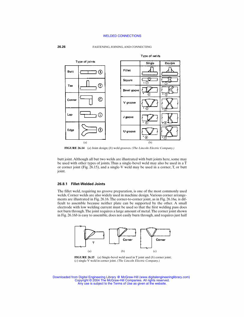
butt joint. Although all but two welds are illustrated with butt joints here, some maybe used with other types of joints. Thus a single-bevel weld may also be used in a Tor corner joint (Fig. 26.15), and a single-V weld may be used in a corner, T, or buttjoint.
26.8.1 Fillet-Welded Joints
The fillet weld, requiring no groove preparation, is one of the most commonly usedwelds. Corner welds are also widely used in machine design.Various corner arrange-ments are illustrated in Fig. 26.16. The corner-to-corner joint, as in Fig. 26.16a, is dif-ficult to assemble because neither plate can be supported by the other. A smallelectrode with low welding current must be used so that the first welding pass doesnot burn through.The joint requires a large amount of metal.The corner joint shownin Fig. 26.16b is easy to assemble, does not easily burn through, and requires just half
26.26 FASTENING, JOINING, AND CONNECTING
FIGURE 26.14 (a) Joint design; (b) weld grooves. (The Lincoln Electric Company.)
FIGURE 26.15 (a) Single-bevel weld used in T joint and (b) corner joint;(c) single-V weld in corner joint. (The Lincoln Electric Company.)
(a) (b)
(a) (b) (c)
WELDED CONNECTIONS
Downloaded from Digital Engineering Library @ McGraw-Hill (www.digitalengineeringlibrary.com)Copyright © 2004 The McGraw-Hill Companies. All rights reserved.
Any use is subject to the Terms of Use as given at the website.
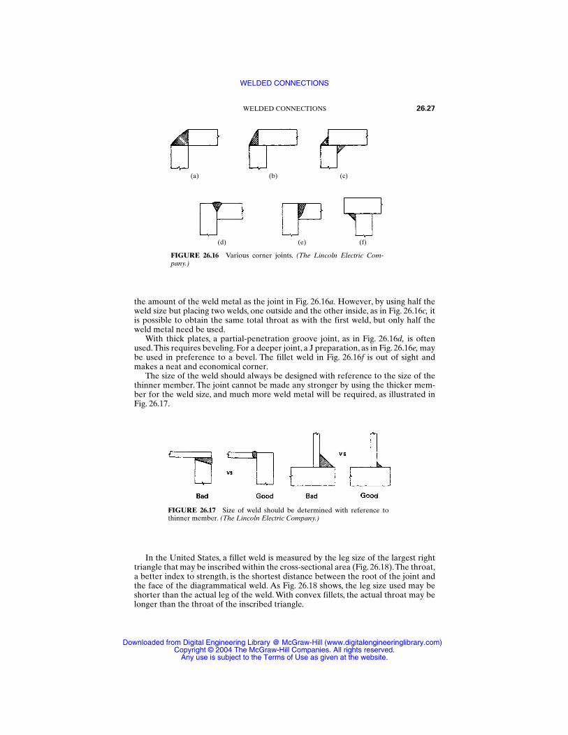
the amount of the weld metal as the joint in Fig. 26.16a. However, by using half theweld size but placing two welds, one outside and the other inside, as in Fig. 26.16c, itis possible to obtain the same total throat as with the first weld, but only half theweld metal need be used.
With thick plates, a partial-penetration groove joint, as in Fig. 26.16d, is oftenused.This requires beveling. For a deeper joint, a J preparation, as in Fig. 26.16e, maybe used in preference to a bevel. The fillet weld in Fig. 26.16f is out of sight andmakes a neat and economical corner.
The size of the weld should always be designed with reference to the size of thethinner member. The joint cannot be made any stronger by using the thicker mem-ber for the weld size, and much more weld metal will be required, as illustrated inFig. 26.17.
In the United States, a fillet weld is measured by the leg size of the largest righttriangle that may be inscribed within the cross-sectional area (Fig. 26.18).The throat,a better index to strength, is the shortest distance between the root of the joint andthe face of the diagrammatical weld. As Fig. 26.18 shows, the leg size used may beshorter than the actual leg of the weld. With convex fillets, the actual throat may belonger than the throat of the inscribed triangle.
WELDED CONNECTIONS 26.27
FIGURE 26.17 Size of weld should be determined with reference tothinner member. (The Lincoln Electric Company.)
(a) (b) (c)
FIGURE 26.16 Various corner joints. (The Lincoln Electric Com-pany.)
(d) (e) (f)
WELDED CONNECTIONS
Downloaded from Digital Engineering Library @ McGraw-Hill (www.digitalengineeringlibrary.com)Copyright © 2004 The McGraw-Hill Companies. All rights reserved.
Any use is subject to the Terms of Use as given at the website.
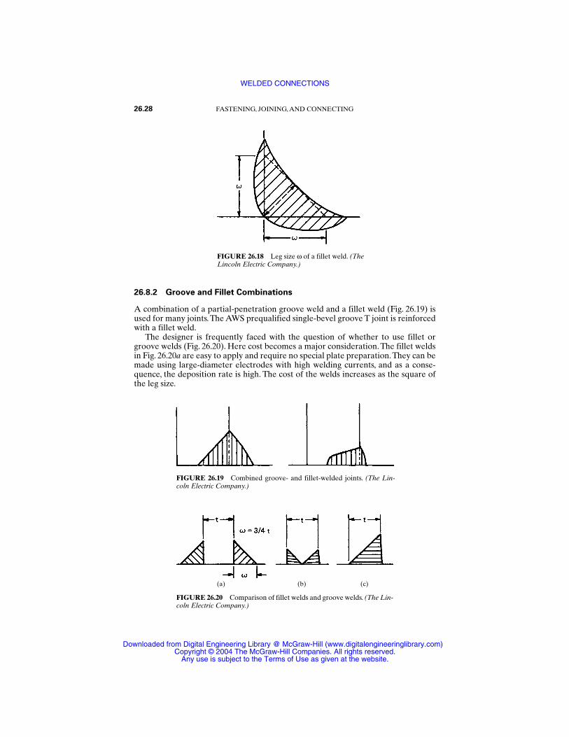
26.8.2 Groove and Fillet Combinations
A combination of a partial-penetration groove weld and a fillet weld (Fig. 26.19) isused for many joints.The AWS prequalified single-bevel groove T joint is reinforcedwith a fillet weld.
The designer is frequently faced with the question of whether to use fillet orgroove welds (Fig. 26.20). Here cost becomes a major consideration. The fillet weldsin Fig. 26.20a are easy to apply and require no special plate preparation.They can bemade using large-diameter electrodes with high welding currents, and as a conse-quence, the deposition rate is high. The cost of the welds increases as the square ofthe leg size.
26.28 FASTENING, JOINING, AND CONNECTING
FIGURE 26.19 Combined groove- and fillet-welded joints. (The Lin-coln Electric Company.)
FIGURE 26.20 Comparison of fillet welds and groove welds. (The Lin-coln Electric Company.)
FIGURE 26.18 Leg size ω of a fillet weld. (TheLincoln Electric Company.)
(a) (b) (c)
WELDED CONNECTIONS
Downloaded from Digital Engineering Library @ McGraw-Hill (www.digitalengineeringlibrary.com)Copyright © 2004 The McGraw-Hill Companies. All rights reserved.
Any use is subject to the Terms of Use as given at the website.
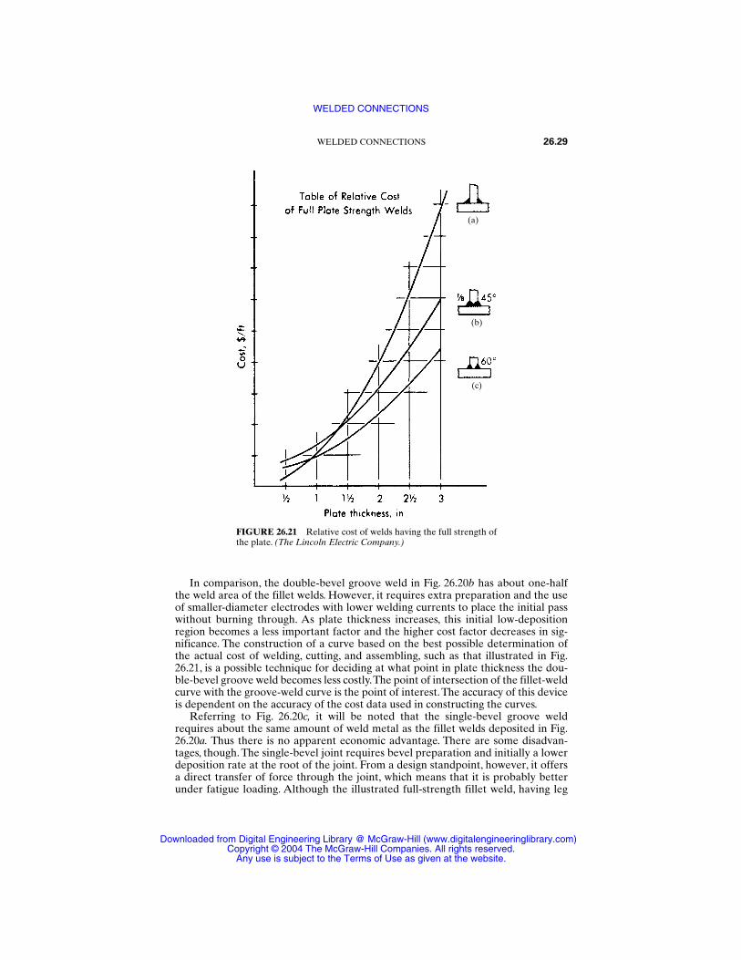
In comparison, the double-bevel groove weld in Fig. 26.20b has about one-halfthe weld area of the fillet welds. However, it requires extra preparation and the useof smaller-diameter electrodes with lower welding currents to place the initial passwithout burning through. As plate thickness increases, this initial low-depositionregion becomes a less important factor and the higher cost factor decreases in sig-nificance. The construction of a curve based on the best possible determination ofthe actual cost of welding, cutting, and assembling, such as that illustrated in Fig.26.21, is a possible technique for deciding at what point in plate thickness the dou-ble-bevel groove weld becomes less costly.The point of intersection of the fillet-weldcurve with the groove-weld curve is the point of interest.The accuracy of this deviceis dependent on the accuracy of the cost data used in constructing the curves.
Referring to Fig. 26.20c, it will be noted that the single-bevel groove weldrequires about the same amount of weld metal as the fillet welds deposited in Fig.26.20a. Thus there is no apparent economic advantage. There are some disadvan-tages, though. The single-bevel joint requires bevel preparation and initially a lowerdeposition rate at the root of the joint. From a design standpoint, however, it offersa direct transfer of force through the joint, which means that it is probably betterunder fatigue loading. Although the illustrated full-strength fillet weld, having leg
WELDED CONNECTIONS 26.29
FIGURE 26.21 Relative cost of welds having the full strength ofthe plate. (The Lincoln Electric Company.)
(a)
(b)
(c)
WELDED CONNECTIONS
Downloaded from Digital Engineering Library @ McGraw-Hill (www.digitalengineeringlibrary.com)Copyright © 2004 The McGraw-Hill Companies. All rights reserved.
Any use is subject to the Terms of Use as given at the website.
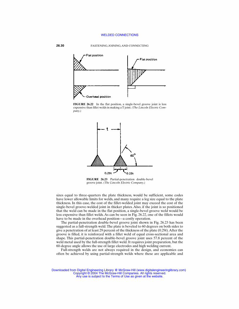
sizes equal to three-quarters the plate thickness, would be sufficient, some codeshave lower allowable limits for welds, and many require a leg size equal to the platethickness. In this case, the cost of the fillet-welded joint may exceed the cost of thesingle-bevel groove-welded joint in thicker plates. Also, if the joint is so positionedthat the weld can be made in the flat position, a single-bevel groove weld would beless expensive than fillet welds. As can be seen in Fig. 26.22, one of the fillets wouldhave to be made in the overhead position—a costly operation.
The partial-penetration double-bevel groove joint shown in Fig. 26.23 has beensuggested as a full-strength weld. The plate is beveled to 60 degrees on both sides togive a penetration of at least 29 percent of the thickness of the plate (0.29t).After thegroove is filled, it is reinforced with a fillet weld of equal cross-sectional area andshape. This partial-penetration double-bevel groove joint uses 57.8 percent of theweld metal used by the full-strength fillet weld. It requires joint preparation, but the60-degree angle allows the use of large electrodes and high welding current.
Full-strength welds are not always required in the design, and economies canoften be achieved by using partial-strength welds where these are applicable and
26.30 FASTENING, JOINING, AND CONNECTING
FIGURE 26.22 In the flat position, a single-bevel groove joint is lessexpensive than fillet welds in making a T joint. (The Lincoln Electric Com-pany.)
FIGURE 26.23 Partial-penetration double-bevelgroove joint. (The Lincoln Electric Company.)
WELDED CONNECTIONS
Downloaded from Digital Engineering Library @ McGraw-Hill (www.digitalengineeringlibrary.com)Copyright © 2004 The McGraw-Hill Companies. All rights reserved.
Any use is subject to the Terms of Use as given at the website.
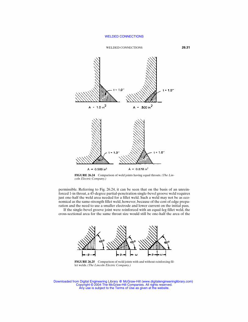
permissible. Referring to Fig. 26.24, it can be seen that on the basis of an unrein-forced 1-in throat, a 45-degree partial-penetration single-bevel groove weld requiresjust one-half the weld area needed for a fillet weld. Such a weld may not be as eco-nomical as the same-strength fillet weld, however, because of the cost of edge prepa-ration and the need to use a smaller electrode and lower current on the initial pass.
If the single-bevel groove joint were reinforced with an equal-leg fillet weld, thecross-sectional area for the same throat size would still be one-half the area of the
WELDED CONNECTIONS 26.31
FIGURE 26.24 Comparison of weld joints having equal throats. (The Lin-coln Electric Company.)
FIGURE 26.25 Comparison of weld joints with and without reinforcing fil-let welds. (The Lincoln Electric Company.)
WELDED CONNECTIONS
Downloaded from Digital Engineering Library @ McGraw-Hill (www.digitalengineeringlibrary.com)Copyright © 2004 The McGraw-Hill Companies. All rights reserved.
Any use is subject to the Terms of Use as given at the website.
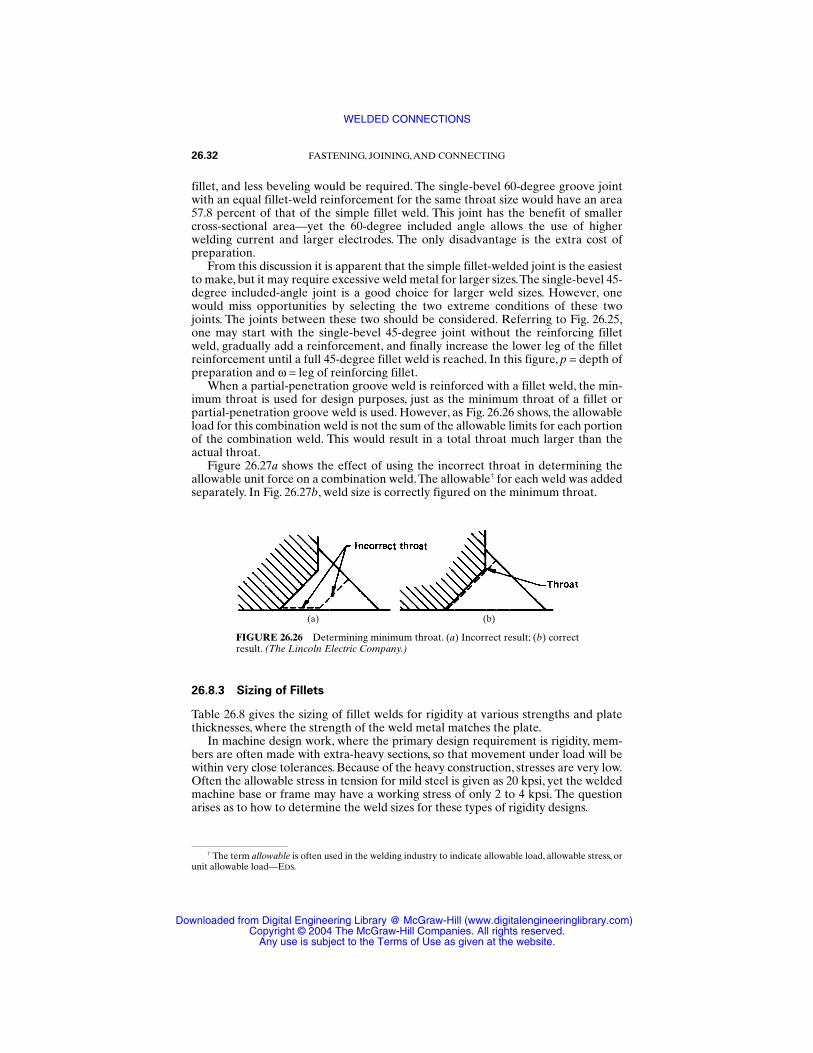
fillet, and less beveling would be required. The single-bevel 60-degree groove jointwith an equal fillet-weld reinforcement for the same throat size would have an area57.8 percent of that of the simple fillet weld. This joint has the benefit of smallercross-sectional area—yet the 60-degree included angle allows the use of higherwelding current and larger electrodes. The only disadvantage is the extra cost ofpreparation.
From this discussion it is apparent that the simple fillet-welded joint is the easiestto make, but it may require excessive weld metal for larger sizes.The single-bevel 45-degree included-angle joint is a good choice for larger weld sizes. However, onewould miss opportunities by selecting the two extreme conditions of these twojoints. The joints between these two should be considered. Referring to Fig. 26.25,one may start with the single-bevel 45-degree joint without the reinforcing filletweld, gradually add a reinforcement, and finally increase the lower leg of the filletreinforcement until a full 45-degree fillet weld is reached. In this figure, p = depth ofpreparation and ω = leg of reinforcing fillet.
When a partial-penetration groove weld is reinforced with a fillet weld, the min-imum throat is used for design purposes, just as the minimum throat of a fillet or partial-penetration groove weld is used. However, as Fig. 26.26 shows, the allowableload for this combination weld is not the sum of the allowable limits for each portionof the combination weld. This would result in a total throat much larger than theactual throat.
Figure 26.27a shows the effect of using the incorrect throat in determining theallowable unit force on a combination weld.The allowable† for each weld was addedseparately. In Fig. 26.27b, weld size is correctly figured on the minimum throat.
26.8.3 Sizing of Fillets
Table 26.8 gives the sizing of fillet welds for rigidity at various strengths and platethicknesses, where the strength of the weld metal matches the plate.
In machine design work, where the primary design requirement is rigidity, mem-bers are often made with extra-heavy sections, so that movement under load will bewithin very close tolerances. Because of the heavy construction, stresses are very low.Often the allowable stress in tension for mild steel is given as 20 kpsi, yet the weldedmachine base or frame may have a working stress of only 2 to 4 kpsi. The questionarises as to how to determine the weld sizes for these types of rigidity designs.
26.32 FASTENING, JOINING, AND CONNECTING
FIGURE 26.26 Determining minimum throat. (a) Incorrect result; (b) correctresult. (The Lincoln Electric Company.)
† The term allowable is often used in the welding industry to indicate allowable load, allowable stress, orunit allowable load—EDS.
(a) (b)
WELDED CONNECTIONS
Downloaded from Digital Engineering Library @ McGraw-Hill (www.digitalengineeringlibrary.com)Copyright © 2004 The McGraw-Hill Companies. All rights reserved.
Any use is subject to the Terms of Use as given at the website.
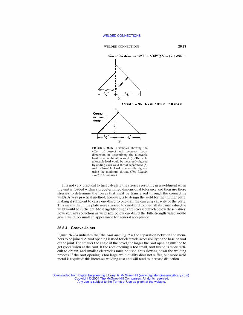
It is not very practical to first calculate the stresses resulting in a weldment whenthe unit is loaded within a predetermined dimensional tolerance and then use thesestresses to determine the forces that must be transferred through the connectingwelds. A very practical method, however, is to design the weld for the thinner plate,making it sufficient to carry one-third to one-half the carrying capacity of the plate.This means that if the plate were stressed to one-third to one-half its usual value, theweld would be sufficient. Most rigidity designs are stressed much below these values;however, any reduction in weld size below one-third the full-strength value wouldgive a weld too small an appearance for general acceptance.
26.8.4 Groove Joints
Figure 26.28a indicates that the root opening R is the separation between the mem-bers to be joined.A root opening is used for electrode accessibility to the base or rootof the joint.The smaller the angle of the bevel, the larger the root opening must be toget good fusion at the root. If the root opening is too small, root fusion is more diffi-cult to obtain, and smaller electrodes must be used, thus slowing down the weldingprocess. If the root opening is too large, weld quality does not suffer, but more weldmetal is required; this increases welding cost and will tend to increase distortion.
WELDED CONNECTIONS 26.33
FIGURE 26.27 Examples showing theeffect of correct and incorrect throatdimension in determining the allowableload on a combination weld. (a) The weldallowable load would be incorrectly figuredby adding each weld throat separately; (b)weld allowable load is correctly figuredusing the minimum throat. (The LincolnElectric Company.)
(b)
(a)
WELDED CONNECTIONS
Downloaded from Digital Engineering Library @ McGraw-Hill (www.digitalengineeringlibrary.com)Copyright © 2004 The McGraw-Hill Companies. All rights reserved.
Any use is subject to the Terms of Use as given at the website.
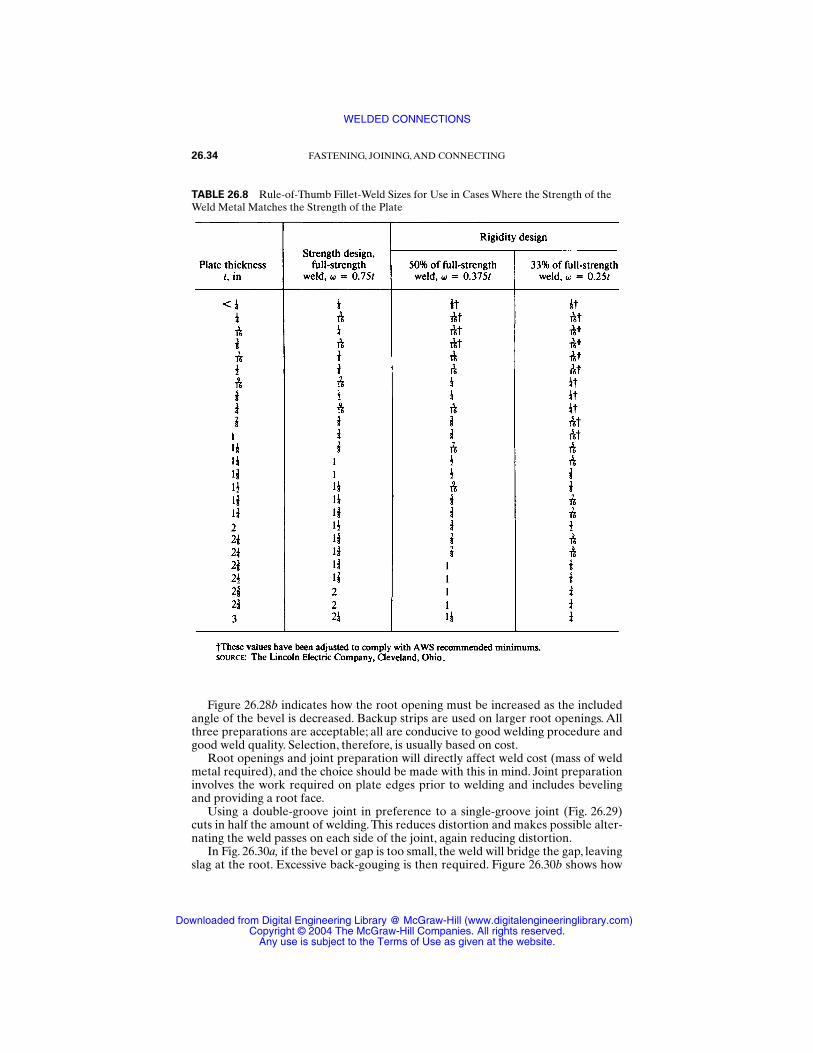
Figure 26.28b indicates how the root opening must be increased as the includedangle of the bevel is decreased. Backup strips are used on larger root openings. Allthree preparations are acceptable; all are conducive to good welding procedure andgood weld quality. Selection, therefore, is usually based on cost.
Root openings and joint preparation will directly affect weld cost (mass of weldmetal required), and the choice should be made with this in mind. Joint preparationinvolves the work required on plate edges prior to welding and includes bevelingand providing a root face.
Using a double-groove joint in preference to a single-groove joint (Fig. 26.29)cuts in half the amount of welding.This reduces distortion and makes possible alter-nating the weld passes on each side of the joint, again reducing distortion.
In Fig. 26.30a, if the bevel or gap is too small, the weld will bridge the gap, leavingslag at the root. Excessive back-gouging is then required. Figure 26.30b shows how
26.34 FASTENING, JOINING, AND CONNECTING
TABLE 26.8 Rule-of-Thumb Fillet-Weld Sizes for Use in Cases Where the Strength of theWeld Metal Matches the Strength of the Plate
WELDED CONNECTIONS
Downloaded from Digital Engineering Library @ McGraw-Hill (www.digitalengineeringlibrary.com)Copyright © 2004 The McGraw-Hill Companies. All rights reserved.
Any use is subject to the Terms of Use as given at the website.
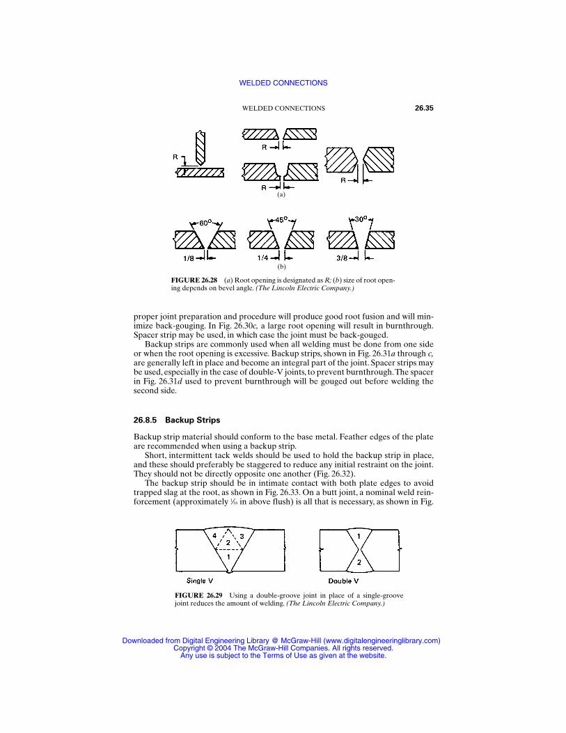
proper joint preparation and procedure will produce good root fusion and will min-imize back-gouging. In Fig. 26.30c, a large root opening will result in burnthrough.Spacer strip may be used, in which case the joint must be back-gouged.
Backup strips are commonly used when all welding must be done from one sideor when the root opening is excessive. Backup strips, shown in Fig. 26.31a through c,are generally left in place and become an integral part of the joint. Spacer strips maybe used, especially in the case of double-V joints, to prevent burnthrough.The spacerin Fig. 26.31d used to prevent burnthrough will be gouged out before welding thesecond side.
26.8.5 Backup Strips
Backup strip material should conform to the base metal. Feather edges of the plateare recommended when using a backup strip.
Short, intermittent tack welds should be used to hold the backup strip in place,and these should preferably be staggered to reduce any initial restraint on the joint.They should not be directly opposite one another (Fig. 26.32).
The backup strip should be in intimate contact with both plate edges to avoidtrapped slag at the root, as shown in Fig. 26.33. On a butt joint, a nominal weld rein-forcement (approximately 1⁄16 in above flush) is all that is necessary, as shown in Fig.
WELDED CONNECTIONS 26.35
FIGURE 26.28 (a) Root opening is designated as R; (b) size of root open-ing depends on bevel angle. (The Lincoln Electric Company.)
(a)
(b)
FIGURE 26.29 Using a double-groove joint in place of a single-groovejoint reduces the amount of welding. (The Lincoln Electric Company.)
WELDED CONNECTIONS
Downloaded from Digital Engineering Library @ McGraw-Hill (www.digitalengineeringlibrary.com)Copyright © 2004 The McGraw-Hill Companies. All rights reserved.
Any use is subject to the Terms of Use as given at the website.
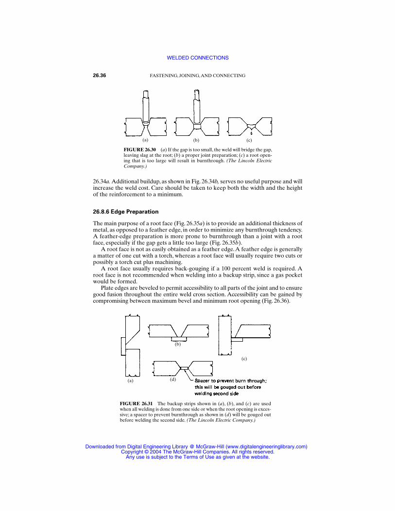
26.34a. Additional buildup, as shown in Fig. 26.34b, serves no useful purpose and willincrease the weld cost. Care should be taken to keep both the width and the heightof the reinforcement to a minimum.
26.8.6 Edge Preparation
The main purpose of a root face (Fig. 26.35a) is to provide an additional thickness ofmetal, as opposed to a feather edge, in order to minimize any burnthrough tendency.A feather-edge preparation is more prone to burnthrough than a joint with a rootface, especially if the gap gets a little too large (Fig. 26.35b).
A root face is not as easily obtained as a feather edge.A feather edge is generallya matter of one cut with a torch, whereas a root face will usually require two cuts orpossibly a torch cut plus machining.
A root face usually requires back-gouging if a 100 percent weld is required. Aroot face is not recommended when welding into a backup strip, since a gas pocketwould be formed.
Plate edges are beveled to permit accessibility to all parts of the joint and to ensuregood fusion throughout the entire weld cross section. Accessibility can be gained bycompromising between maximum bevel and minimum root opening (Fig. 26.36).
26.36 FASTENING, JOINING, AND CONNECTING
FIGURE 26.30 (a) If the gap is too small, the weld will bridge the gap,leaving slag at the root; (b) a proper joint preparation; (c) a root open-ing that is too large will result in burnthrough. (The Lincoln ElectricCompany.)
(a) (b) (c)
FIGURE 26.31 The backup strips shown in (a), (b), and (c) are usedwhen all welding is done from one side or when the root opening is exces-sive; a spacer to prevent burnthrough as shown in (d) will be gouged outbefore welding the second side. (The Lincoln Electric Company.)
(b)
(c)
(a) (d)
WELDED CONNECTIONS
Downloaded from Digital Engineering Library @ McGraw-Hill (www.digitalengineeringlibrary.com)Copyright © 2004 The McGraw-Hill Companies. All rights reserved.
Any use is subject to the Terms of Use as given at the website.
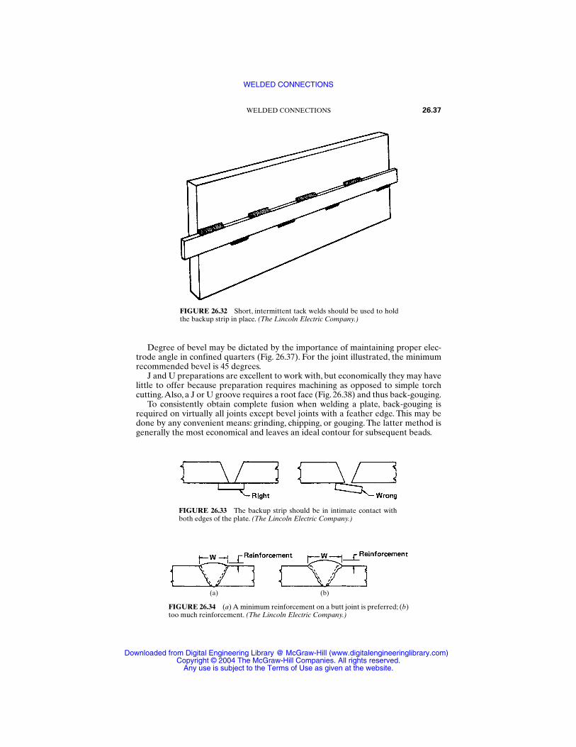
Degree of bevel may be dictated by the importance of maintaining proper elec-trode angle in confined quarters (Fig. 26.37). For the joint illustrated, the minimumrecommended bevel is 45 degrees.
J and U preparations are excellent to work with, but economically they may havelittle to offer because preparation requires machining as opposed to simple torchcutting.Also, a J or U groove requires a root face (Fig. 26.38) and thus back-gouging.
To consistently obtain complete fusion when welding a plate, back-gouging isrequired on virtually all joints except bevel joints with a feather edge. This may bedone by any convenient means: grinding, chipping, or gouging. The latter method isgenerally the most economical and leaves an ideal contour for subsequent beads.
WELDED CONNECTIONS 26.37
FIGURE 26.32 Short, intermittent tack welds should be used to holdthe backup strip in place. (The Lincoln Electric Company.)
FIGURE 26.33 The backup strip should be in intimate contact withboth edges of the plate. (The Lincoln Electric Company.)
FIGURE 26.34 (a) A minimum reinforcement on a butt joint is preferred; (b)too much reinforcement. (The Lincoln Electric Company.)
(a) (b)
WELDED CONNECTIONS
Downloaded from Digital Engineering Library @ McGraw-Hill (www.digitalengineeringlibrary.com)Copyright © 2004 The McGraw-Hill Companies. All rights reserved.
Any use is subject to the Terms of Use as given at the website.
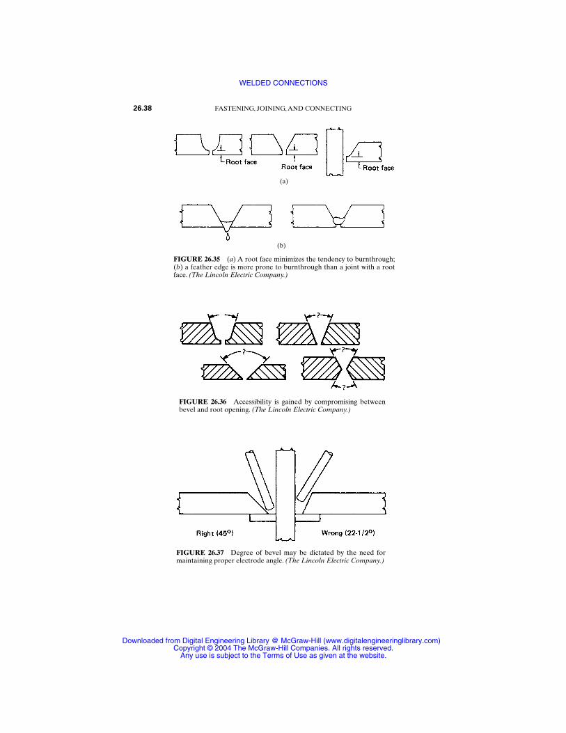
26.38 FASTENING, JOINING, AND CONNECTING
FIGURE 26.35 (a) A root face minimizes the tendency to burnthrough;(b) a feather edge is more prone to burnthrough than a joint with a rootface. (The Lincoln Electric Company.)
(a)
(b)
FIGURE 26.36 Accessibility is gained by compromising betweenbevel and root opening. (The Lincoln Electric Company.)
FIGURE 26.37 Degree of bevel may be dictated by the need formaintaining proper electrode angle. (The Lincoln Electric Company.)
WELDED CONNECTIONS
Downloaded from Digital Engineering Library @ McGraw-Hill (www.digitalengineeringlibrary.com)Copyright © 2004 The McGraw-Hill Companies. All rights reserved.
Any use is subject to the Terms of Use as given at the website.
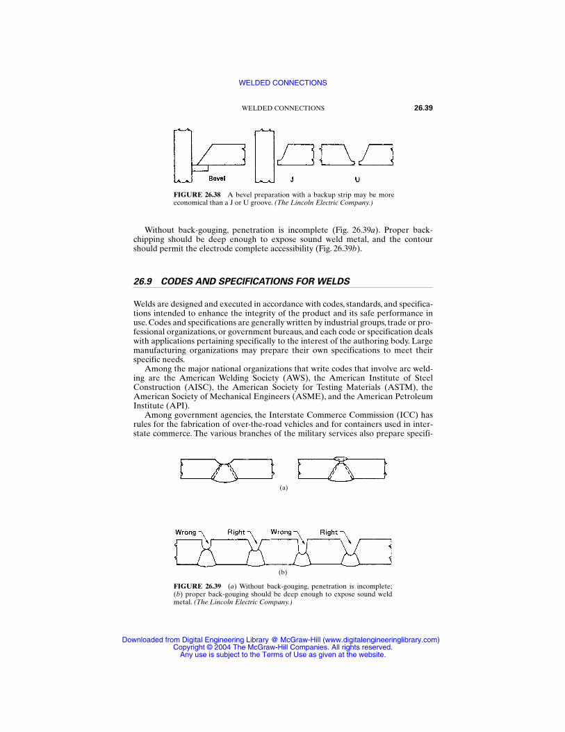
Without back-gouging, penetration is incomplete (Fig. 26.39a). Proper back-chipping should be deep enough to expose sound weld metal, and the contourshould permit the electrode complete accessibility (Fig. 26.39b).
26.9 CODES AND SPECIFICATIONS FOR WELDS
Welds are designed and executed in accordance with codes, standards, and specifica-tions intended to enhance the integrity of the product and its safe performance inuse. Codes and specifications are generally written by industrial groups, trade or pro-fessional organizations, or government bureaus, and each code or specification dealswith applications pertaining specifically to the interest of the authoring body. Largemanufacturing organizations may prepare their own specifications to meet theirspecific needs.
Among the major national organizations that write codes that involve arc weld-ing are the American Welding Society (AWS), the American Institute of Steel Construction (AISC), the American Society for Testing Materials (ASTM), theAmerican Society of Mechanical Engineers (ASME), and the American PetroleumInstitute (API).
Among government agencies, the Interstate Commerce Commission (ICC) hasrules for the fabrication of over-the-road vehicles and for containers used in inter-state commerce. The various branches of the military services also prepare specifi-
WELDED CONNECTIONS 26.39
FIGURE 26.38 A bevel preparation with a backup strip may be moreeconomical than a J or U groove. (The Lincoln Electric Company.)
FIGURE 26.39 (a) Without back-gouging, penetration is incomplete;(b) proper back-gouging should be deep enough to expose sound weldmetal. (The Lincoln Electric Company.)
(b)
(a)
WELDED CONNECTIONS
Downloaded from Digital Engineering Library @ McGraw-Hill (www.digitalengineeringlibrary.com)Copyright © 2004 The McGraw-Hill Companies. All rights reserved.
Any use is subject to the Terms of Use as given at the website.
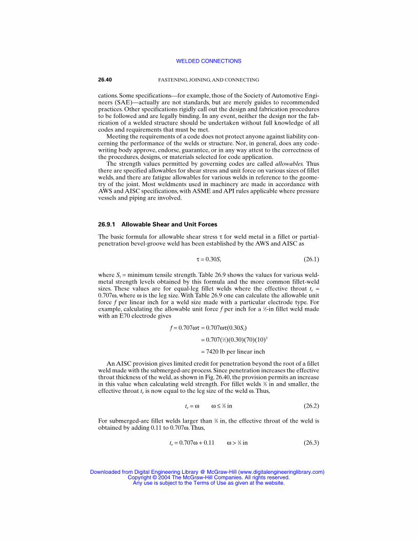
cations. Some specifications—for example, those of the Society of Automotive Engi-neers (SAE)—actually are not standards, but are merely guides to recommendedpractices. Other specifications rigidly call out the design and fabrication proceduresto be followed and are legally binding. In any event, neither the design nor the fab-rication of a welded structure should be undertaken without full knowledge of allcodes and requirements that must be met.
Meeting the requirements of a code does not protect anyone against liability con-cerning the performance of the welds or structure. Nor, in general, does any code-writing body approve, endorse, guarantee, or in any way attest to the correctness ofthe procedures, designs, or materials selected for code application.
The strength values permitted by governing codes are called allowables. Thusthere are specified allowables for shear stress and unit force on various sizes of filletwelds, and there are fatigue allowables for various welds in reference to the geome-try of the joint. Most weldments used in machinery are made in accordance withAWS and AISC specifications, with ASME and API rules applicable where pressurevessels and piping are involved.
26.9.1 Allowable Shear and Unit Forces
The basic formula for allowable shear stress τ for weld metal in a fillet or partial-penetration bevel-groove weld has been established by the AWS and AISC as
τ = 0.30St (26.1)
where St = minimum tensile strength. Table 26.9 shows the values for various weld-metal strength levels obtained by this formula and the more common fillet-weldsizes. These values are for equal-leg fillet welds where the effective throat te =0.707ω, where ω is the leg size. With Table 26.9 one can calculate the allowable unitforce f per linear inch for a weld size made with a particular electrode type. Forexample, calculating the allowable unit force f per inch for a 1⁄2-in fillet weld madewith an E70 electrode gives
f = 0.707ωτ = 0.707ωτ(0.30St)
= 0.707(1⁄2)(0.30)(70)(10)3
= 7420 lb per linear inch
An AISC provision gives limited credit for penetration beyond the root of a filletweld made with the submerged-arc process. Since penetration increases the effectivethroat thickness of the weld, as shown in Fig. 26.40, the provision permits an increasein this value when calculating weld strength. For fillet welds 3⁄8 in and smaller, theeffective throat te is now equal to the leg size of the weld ω. Thus,
te = ω ω ≤ 3⁄8 in (26.2)
For submerged-arc fillet welds larger than 3⁄8 in, the effective throat of the weld isobtained by adding 0.11 to 0.707ω. Thus,
te = 0.707ω + 0.11 ω > 3⁄8 in (26.3)
26.40 FASTENING, JOINING, AND CONNECTING
WELDED CONNECTIONS
Downloaded from Digital Engineering Library @ McGraw-Hill (www.digitalengineeringlibrary.com)Copyright © 2004 The McGraw-Hill Companies. All rights reserved.
Any use is subject to the Terms of Use as given at the website.
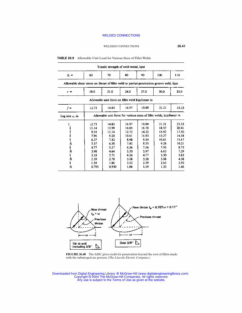
WELDED CONNECTIONS 26.41
TABLE 26.9 Allowable Unit Load for Various Sizes of Fillet Welds
FIGURE 26.40 The AISC gives credit for penetration beyond the root of fillets madewith the submerged-arc process. (The Lincoln Electric Company.)
WELDED CONNECTIONS
Downloaded from Digital Engineering Library @ McGraw-Hill (www.digitalengineeringlibrary.com)Copyright © 2004 The McGraw-Hill Companies. All rights reserved.
Any use is subject to the Terms of Use as given at the website.

where te is in inches. Note that allowance for penetration applies only to fillet weldsmade by the submerged-arc welding process. Electrode polarity will provide thispenetration.
26.9.2 Minimum Fillet-Weld Size
The minimum sizes of fillet welds for specific material thicknesses are shown inTable 26.10. In the AISC Specifications and the AWS Structural Welding Code, thistable has been expanded to include material less than 1⁄4 in thick and 1⁄8-in fillets.Where materials of different thicknesses are being joined, the minimum fillet weldsize is governed by the thicker material, but this size does not have to exceed thethickness of the thinner material unless required by the calculated stress.
26.9.3 Allowables for Weld Metal—A Handy Reference
Table 26.11 summarizes the AWS Structural Welding Code and AISC allowables forweld metal. It is intended to provide a ready reference for picking the properstrength levels for the various types of steels. Once this selection has been made, theallowables can be quickly found for the various types of welds that may be requiredfor the specific assembly.
26.9.4 AISC Fatigue Allowables
The AISC Specifications include fatigue allowables, which also are accepted by theAWS Building Code, Sec. 8. Therefore, designers have something other than theAWS Building Code, Sec. 10, Bridges, with its automatic 10 percent lower allowabledesign stress, on which to base fatigue considerations.
Although developed for structures, these allowables are adaptable to the fatigueproblems of machine-tool makers, equipment manufacturers, and others who fabri-cate with welded steel. They cover a wide range of welded joints and members andnot only provide values for various types of welds, but also take into considerationthe strength of members attached by welds.
26.42 FASTENING, JOINING, AND CONNECTING
TABLE 26.10 Minimum Fillet-Weld Size ωin Inches
WELDED CONNECTIONS
Downloaded from Digital Engineering Library @ McGraw-Hill (www.digitalengineeringlibrary.com)Copyright © 2004 The McGraw-Hill Companies. All rights reserved.
Any use is subject to the Terms of Use as given at the website.
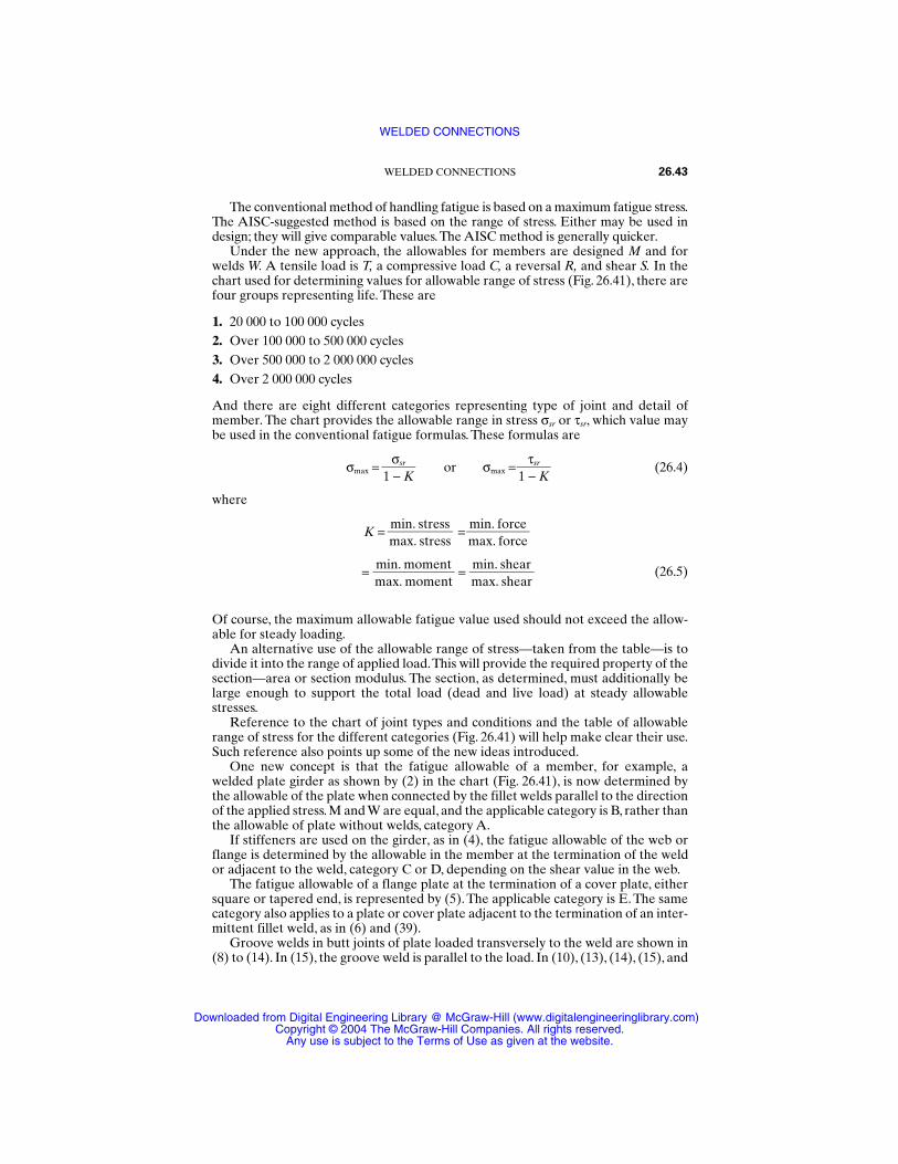
The conventional method of handling fatigue is based on a maximum fatigue stress.The AISC-suggested method is based on the range of stress. Either may be used indesign; they will give comparable values.The AISC method is generally quicker.
Under the new approach, the allowables for members are designed M and forwelds W. A tensile load is T, a compressive load C, a reversal R, and shear S. In thechart used for determining values for allowable range of stress (Fig. 26.41), there arefour groups representing life. These are
1. 20 000 to 100 000 cycles2. Over 100 000 to 500 000 cycles3. Over 500 000 to 2 000 000 cycles4. Over 2 000 000 cycles
And there are eight different categories representing type of joint and detail ofmember. The chart provides the allowable range in stress σsr or τsr, which value maybe used in the conventional fatigue formulas. These formulas are
σmax = or σmax = (26.4)
where
K = =
(26.5)= =
Of course, the maximum allowable fatigue value used should not exceed the allow-able for steady loading.
An alternative use of the allowable range of stress—taken from the table—is todivide it into the range of applied load.This will provide the required property of thesection—area or section modulus. The section, as determined, must additionally belarge enough to support the total load (dead and live load) at steady allowablestresses.
Reference to the chart of joint types and conditions and the table of allowablerange of stress for the different categories (Fig. 26.41) will help make clear their use.Such reference also points up some of the new ideas introduced.
One new concept is that the fatigue allowable of a member, for example, awelded plate girder as shown by (2) in the chart (Fig. 26.41), is now determined bythe allowable of the plate when connected by the fillet welds parallel to the directionof the applied stress. M and W are equal, and the applicable category is B, rather thanthe allowable of plate without welds, category A.
If stiffeners are used on the girder, as in (4), the fatigue allowable of the web orflange is determined by the allowable in the member at the termination of the weldor adjacent to the weld, category C or D, depending on the shear value in the web.
The fatigue allowable of a flange plate at the termination of a cover plate, eithersquare or tapered end, is represented by (5). The applicable category is E. The samecategory also applies to a plate or cover plate adjacent to the termination of an inter-mittent fillet weld, as in (6) and (39).
Groove welds in butt joints of plate loaded transversely to the weld are shown in(8) to (14). In (15), the groove weld is parallel to the load. In (10), (13), (14), (15), and
min. shearmax. shear
min. momentmax. moment
min. forcemax. force
min. stressmax. stress
τsr1 − K
σsr1 − K
WELDED CONNECTIONS 26.43
WELDED CONNECTIONS
Downloaded from Digital Engineering Library @ McGraw-Hill (www.digitalengineeringlibrary.com)Copyright © 2004 The McGraw-Hill Companies. All rights reserved.
Any use is subject to the Terms of Use as given at the website.
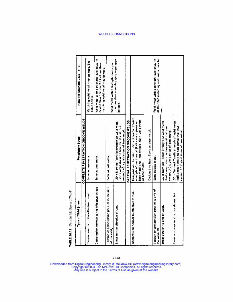
TA
BLE
26.1
1P
erm
issi
ble
Stre
ss o
f Wel
d†
26.44
WELDED CONNECTIONS
Downloaded from Digital Engineering Library @ McGraw-Hill (www.digitalengineeringlibrary.com)Copyright © 2004 The McGraw-Hill Companies. All rights reserved.
Any use is subject to the Terms of Use as given at the website.
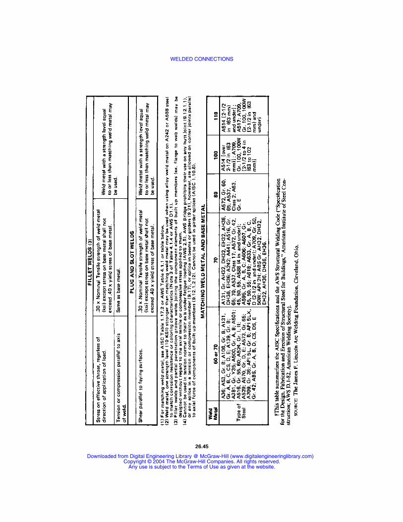
26.45
WELDED CONNECTIONS
Downloaded from Digital Engineering Library @ McGraw-Hill (www.digitalengineeringlibrary.com)Copyright © 2004 The McGraw-Hill Companies. All rights reserved.
Any use is subject to the Terms of Use as given at the website.

26.46 FASTENING, JOINING, AND CONNECTING
FIGURE 26.41 The AISC allowable range of stress σsr or τsr. (The Lincoln Electric Company.)
WELDED CONNECTIONS
Downloaded from Digital Engineering Library @ McGraw-Hill (www.digitalengineeringlibrary.com)Copyright © 2004 The McGraw-Hill Companies. All rights reserved.
Any use is subject to the Terms of Use as given at the website.

WELDED CONNECTIONS 26.47
FIGURE 26.41 (Continued) The AISC allowable range of stress σsr or τsr. (The Lincoln ElectricCompany.)
WELDED CONNECTIONS
Downloaded from Digital Engineering Library @ McGraw-Hill (www.digitalengineeringlibrary.com)Copyright © 2004 The McGraw-Hill Companies. All rights reserved.
Any use is subject to the Terms of Use as given at the website.
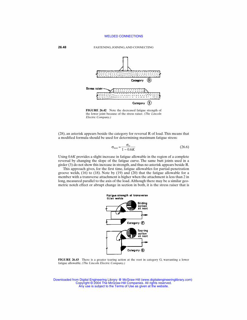
(28), an asterisk appears beside the category for reversal R of load. This means thata modified formula should be used for determining maximum fatigue stress:
σmax = (26.6)
Using 0.6K provides a slight increase in fatigue allowable in the region of a completereversal by changing the slope of the fatigue curve. The same butt joints used in agirder (3) do not show this increase in strength, and thus no asterisk appears beside R.
This approach gives, for the first time, fatigue allowables for partial-penetrationgroove welds, (16) to (18). Note by (19) and (20) that the fatigue allowable for amember with a transverse attachment is higher when the attachment is less than 2 inlong, measured parallel to the axis of the load.Although there may be a similar geo-metric notch effect or abrupt change in section in both, it is the stress raiser that is
σsr1 − 0.6K
26.48 FASTENING, JOINING, AND CONNECTING
FIGURE 26.42 Note the decreased fatigue strength ofthe lower joint because of the stress raiser. (The LincolnElectric Company.)
FIGURE 26.43 There is a greater tearing action at the root in category G, warranting a lowerfatigue allowable. (The Lincoln Electric Company.)
WELDED CONNECTIONS
Downloaded from Digital Engineering Library @ McGraw-Hill (www.digitalengineeringlibrary.com)Copyright © 2004 The McGraw-Hill Companies. All rights reserved.
Any use is subject to the Terms of Use as given at the website.

important.The transverse bar in (19) is so short as far as the axis of the member andload are concerned that very little of the force is able to swing up and into the barand then back down again. Consequently, the stress raiser is not severe. The longerbar attachment in (20), however, is sufficiently long to provide a path for the forcethrough it and the connecting welds. Because of this force transfer through thewelds, there will be a higher stress raiser and, as a result, a reduction of the fatiguestrength of the member. The difference is illustrated in Fig. 26.42.
Item (30) of the chart, which falls into category E, should not be confused with(37), category G. Both depict transverse fillet welds, but (30) provides a fatigueallowable for the member adjacent to the fillet weld, whereas (37) provides a fatigueshear allowable for the throat of the fillet weld.
Knowing that the steady strength of a transverse fillet is about a third strongerthan that of a parallel fillet, one might question why the fatigue allowable for a par-allel fillet, (34) and (35), category F, is the same as that for a transverse fillet (36) andhigher than that for a transverse fillet (37), category G. The fatigue strength of thetransverse fillet (36) is actually higher than that of a parallel fillet (34), but they bothfall into the range covered by category F. However, there is a difference in the twotransverse fillet welds in (36) and (37). In (36) there may be a slight stress raiserbecause of the pinching together of forces as they pass through the weld. But in (37)there is a greater tearing action at the root of the weld, thus producing a lower fatiguestrength and warranting a lower fatigue allowable. This is illustrated by Fig. 26.43.
WELDED CONNECTIONS 26.49
WELDED CONNECTIONS
Downloaded from Digital Engineering Library @ McGraw-Hill (www.digitalengineeringlibrary.com)Copyright © 2004 The McGraw-Hill Companies. All rights reserved.
Any use is subject to the Terms of Use as given at the website.

WELDED CONNECTIONS
Downloaded from Digital Engineering Library @ McGraw-Hill (www.digitalengineeringlibrary.com)Copyright © 2004 The McGraw-Hill Companies. All rights reserved.
Any use is subject to the Terms of Use as given at the website.

CHAPTER 27FITS AND TOLERANCES
Joseph E. ShigleyProfessor Emeritus
The University of MichiganAnn Arbor, Michigan
Charles R. Mischke, Ph.D., P.E.Professor Emeritus of Mechanical Engineering
Iowa State UniversityAmes, Iowa
27.1 INTRODUCTION / 27.2
27.2 METRIC STANDARDS / 27.2
27.3 U.S. STANDARD—INCH UNITS / 27.9
27.4 INTERFERENCE-FIT STRESSES / 27.9
27.5 ABSOLUTE TOLERANCES / 27.13
REFERENCES / 27.16
NOMENCLATURE
a RadiusB Smallest bore diameterb Radiusc Radius radial clearanceD Diameter, mean of size range, largest journal diameterE Young’s moduluse Bilateral tolerance expressing errorL Upper or lower limitp Probabilitypf Probability of failuret Bilateral tolerance of dimensionw Left-tending vector representing gapx Right-tending dimensional vector magnitudey Left-tending dimensional vector magnitudeδ Radial interferenceυ Poisson’s ratioσ Normal stressç Standard deviation
27.1
Source: STANDARD HANDBOOK OF MACHINE DESIGN
Downloaded from Digital Engineering Library @ McGraw-Hill (www.digitalengineeringlibrary.com)Copyright © 2004 The McGraw-Hill Companies. All rights reserved.
Any use is subject to the Terms of Use as given at the website.
27.1 INTRODUCTION
Standards of limits and fits for mating parts have been approved for general use inthe United States for use with U.S. customary units [27.1] and for use with SI units[27.2]. The tables included in these standards are so lengthy that formulas are pre-sented here instead of the tables to save space. As a result of rounding and othervariations, the formulas are only close approximations. The nomenclature and sym-bols used in the two standards differ from each other, and so it is necessary topresent the details of each standard separately.
27.2 METRIC STANDARDS
27.2.1 Definitions
Terms used are illustrated in Fig. 27.1 and are defined as follows:
1. Basic size is the size to which limits or deviations are assigned and is the same forboth members of a fit. It is measured in millimeters.
2. Deviation is the algebraic difference between a size and the corresponding basicsize.
3. Upper deviation is the algebraic difference between the maximum limit and thecorresponding basic size.
4. Lower deviation is the algebraic difference between the minimum limit and thecorresponding basic size.
5. Fundamental deviation is either the upper or the lower deviation, depending onwhich is closest to the basic size.
6. Tolerance is the difference between the maximum and minimum size limits of apart.
7. International tolerance grade (IT) is a group of tolerances which have the samerelative level of accuracy but which vary depending on the basic size.
8. Hole basis represents a system of fits corresponding to a basic hole size.9. Shaft basis represents a system of fits corresponding to a basic shaft size.
27.2.2 International Tolerance Grades
The variation in part size, also called the magnitude of the tolerance zone, isexpressed in grade or IT numbers. Seven grade numbers are used for high-precisionparts; these are
IT01, IT0, IT1, IT2, IT3, IT4, IT5
The most commonly used grade numbers are IT6 through IT16, and these are basedon the Renard R5 geometric series of numbers. For these, the basic equation is
i = 10
100 (0.45D1/3 + 0.001D) (27.1)
27.2 FASTENING, JOINING, AND CONNECTING
FITS AND TOLERANCES
Downloaded from Digital Engineering Library @ McGraw-Hill (www.digitalengineeringlibrary.com)Copyright © 2004 The McGraw-Hill Companies. All rights reserved.
Any use is subject to the Terms of Use as given at the website.
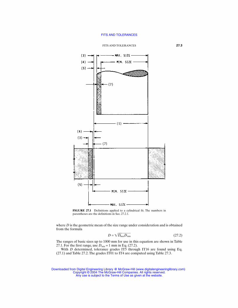
where D is the geometric mean of the size range under consideration and is obtainedfrom the formula
D = DmaxDmin (27.2)
The ranges of basic sizes up to 1000 mm for use in this equation are shown in Table27.1. For the first range, use Dmin = 1 mm in Eq. (27.2).
With D determined, tolerance grades IT5 through IT16 are found using Eq.(27.1) and Table 27.2. The grades IT01 to IT4 are computed using Table 27.3.
FITS AND TOLERANCES 27.3
FIGURE 27.1 Definitions applied to a cylindrical fit. The numbers inparentheses are the definitions in Sec. 27.2.1.
FITS AND TOLERANCES
Downloaded from Digital Engineering Library @ McGraw-Hill (www.digitalengineeringlibrary.com)Copyright © 2004 The McGraw-Hill Companies. All rights reserved.
Any use is subject to the Terms of Use as given at the website.
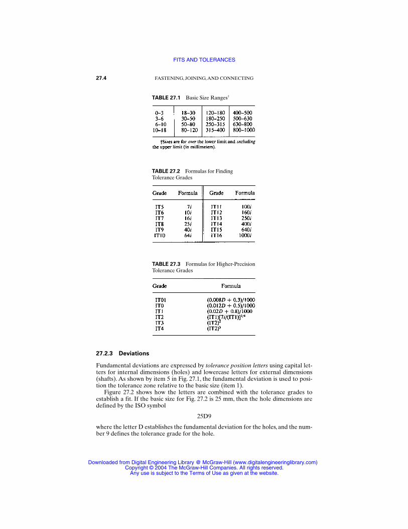
27.2.3 Deviations
Fundamental deviations are expressed by tolerance position letters using capital let-ters for internal dimensions (holes) and lowercase letters for external dimensions(shafts). As shown by item 5 in Fig. 27.1, the fundamental deviation is used to posi-tion the tolerance zone relative to the basic size (item 1).
Figure 27.2 shows how the letters are combined with the tolerance grades toestablish a fit. If the basic size for Fig. 27.2 is 25 mm, then the hole dimensions aredefined by the ISO symbol
25D9
where the letter D establishes the fundamental deviation for the holes, and the num-ber 9 defines the tolerance grade for the hole.
27.4 FASTENING, JOINING, AND CONNECTING
TABLE 27.1 Basic Size Ranges†
TABLE 27.2 Formulas for Finding Tolerance Grades
TABLE 27.3 Formulas for Higher-PrecisionTolerance Grades
FITS AND TOLERANCES
Downloaded from Digital Engineering Library @ McGraw-Hill (www.digitalengineeringlibrary.com)Copyright © 2004 The McGraw-Hill Companies. All rights reserved.
Any use is subject to the Terms of Use as given at the website.
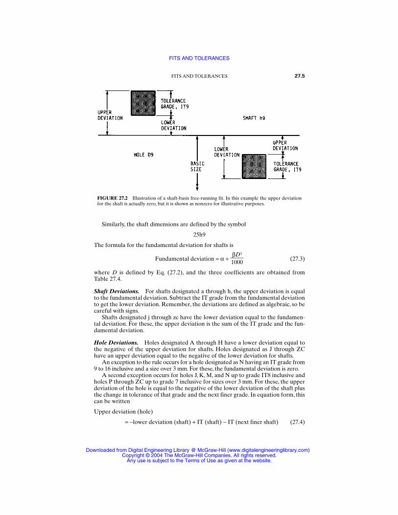
Similarly, the shaft dimensions are defined by the symbol
25h9
The formula for the fundamental deviation for shafts is
Fundamental deviation = α + (27.3)
where D is defined by Eq. (27.2), and the three coefficients are obtained fromTable 27.4.
Shaft Deviations. For shafts designated a through h, the upper deviation is equalto the fundamental deviation. Subtract the IT grade from the fundamental deviationto get the lower deviation. Remember, the deviations are defined as algebraic, so becareful with signs.
Shafts designated j through zc have the lower deviation equal to the fundamen-tal deviation. For these, the upper deviation is the sum of the IT grade and the fun-damental deviation.
Hole Deviations. Holes designated A through H have a lower deviation equal tothe negative of the upper deviation for shafts. Holes designated as J through ZChave an upper deviation equal to the negative of the lower deviation for shafts.
An exception to the rule occurs for a hole designated as N having an IT grade from9 to 16 inclusive and a size over 3 mm. For these, the fundamental deviation is zero.
A second exception occurs for holes J, K, M, and N up to grade IT8 inclusive andholes P through ZC up to grade 7 inclusive for sizes over 3 mm. For these, the upperdeviation of the hole is equal to the negative of the lower deviation of the shaft plusthe change in tolerance of that grade and the next finer grade. In equation form, thiscan be written
Upper deviation (hole)
= −lower deviation (shaft) + IT (shaft) − IT (next finer shaft) (27.4)
βDγ
1000
FITS AND TOLERANCES 27.5
FIGURE 27.2 Illustration of a shaft-basis free-running fit. In this example the upper deviationfor the shaft is actually zero, but it is shown as nonzero for illustrative purposes.
FITS AND TOLERANCES
Downloaded from Digital Engineering Library @ McGraw-Hill (www.digitalengineeringlibrary.com)Copyright © 2004 The McGraw-Hill Companies. All rights reserved.
Any use is subject to the Terms of Use as given at the website.
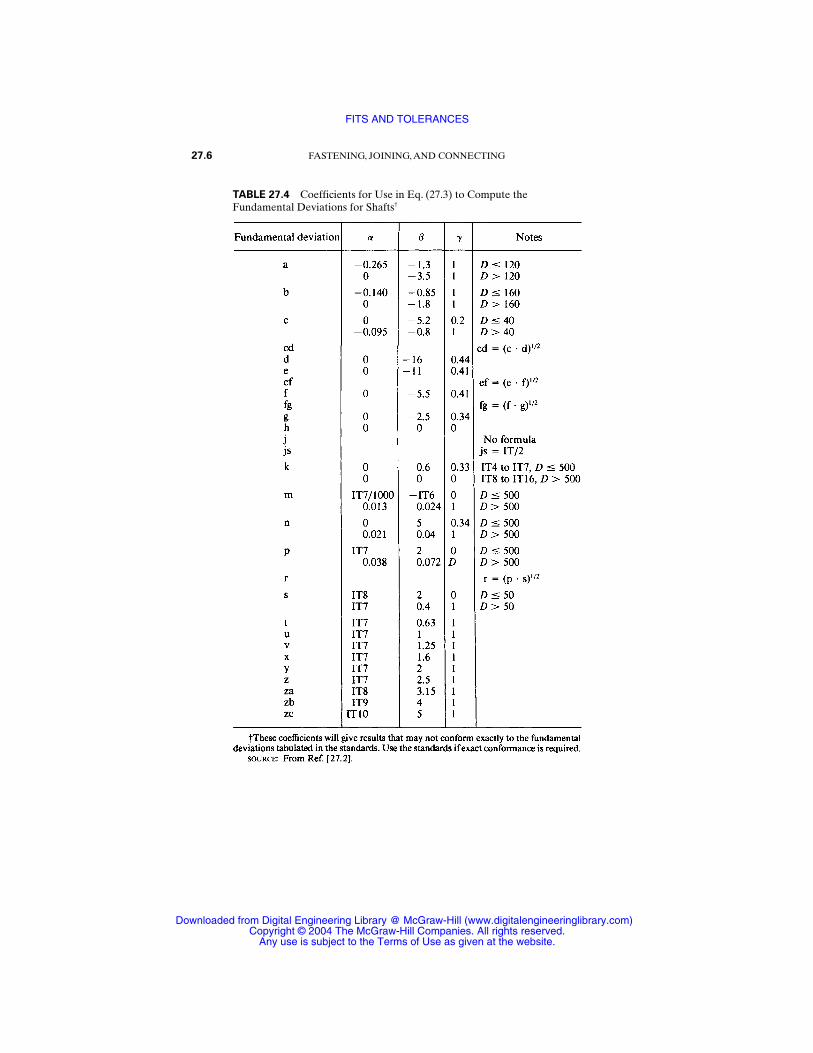
27.6 FASTENING, JOINING, AND CONNECTING
TABLE 27.4 Coefficients for Use in Eq. (27.3) to Compute the Fundamental Deviations for Shafts†
FITS AND TOLERANCES
Downloaded from Digital Engineering Library @ McGraw-Hill (www.digitalengineeringlibrary.com)Copyright © 2004 The McGraw-Hill Companies. All rights reserved.
Any use is subject to the Terms of Use as given at the website.

FITS AND TOLERANCES 27.7
TABLE 27.5 Preferred Fits
FITS AND TOLERANCES
Downloaded from Digital Engineering Library @ McGraw-Hill (www.digitalengineeringlibrary.com)Copyright © 2004 The McGraw-Hill Companies. All rights reserved.
Any use is subject to the Terms of Use as given at the website.
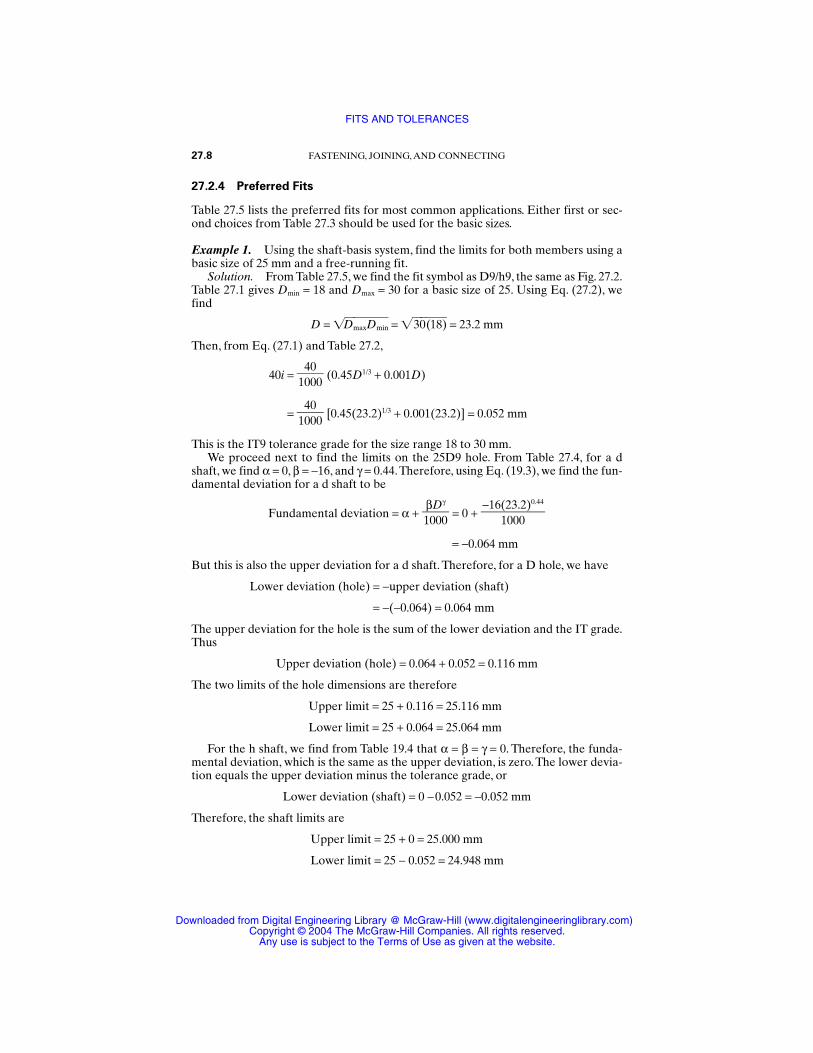
27.2.4 Preferred Fits
Table 27.5 lists the preferred fits for most common applications. Either first or sec-ond choices from Table 27.3 should be used for the basic sizes.
Example 1. Using the shaft-basis system, find the limits for both members using abasic size of 25 mm and a free-running fit.
Solution. From Table 27.5, we find the fit symbol as D9/h9, the same as Fig. 27.2.Table 27.1 gives Dmin = 18 and Dmax = 30 for a basic size of 25. Using Eq. (27.2), wefind
D = DmaxDmin = 30(18) = 23.2 mm
Then, from Eq. (27.1) and Table 27.2,
40i = 140000 (0.45D1/3 + 0.001D)
= 140000 [0.45(23.2)1/3 + 0.001(23.2)] = 0.052 mm
This is the IT9 tolerance grade for the size range 18 to 30 mm.We proceed next to find the limits on the 25D9 hole. From Table 27.4, for a d
shaft, we find α = 0, β = −16, and γ = 0.44.Therefore, using Eq. (19.3), we find the fun-damental deviation for a d shaft to be
Fundamental deviation = α + = 0 +
= −0.064 mm
But this is also the upper deviation for a d shaft. Therefore, for a D hole, we have
Lower deviation (hole) = −upper deviation (shaft)
= −(−0.064) = 0.064 mm
The upper deviation for the hole is the sum of the lower deviation and the IT grade.Thus
Upper deviation (hole) = 0.064 + 0.052 = 0.116 mm
The two limits of the hole dimensions are therefore
Upper limit = 25 + 0.116 = 25.116 mm
Lower limit = 25 + 0.064 = 25.064 mm
For the h shaft, we find from Table 19.4 that α = β = γ = 0. Therefore, the funda-mental deviation, which is the same as the upper deviation, is zero. The lower devia-tion equals the upper deviation minus the tolerance grade, or
Lower deviation (shaft) = 0 −0.052 = −0.052 mm
Therefore, the shaft limits are
Upper limit = 25 + 0 = 25.000 mm
Lower limit = 25 − 0.052 = 24.948 mm
−16(23.2)0.44
1000
βDγ
1000
27.8 FASTENING, JOINING, AND CONNECTING
FITS AND TOLERANCES
Downloaded from Digital Engineering Library @ McGraw-Hill (www.digitalengineeringlibrary.com)Copyright © 2004 The McGraw-Hill Companies. All rights reserved.
Any use is subject to the Terms of Use as given at the website.
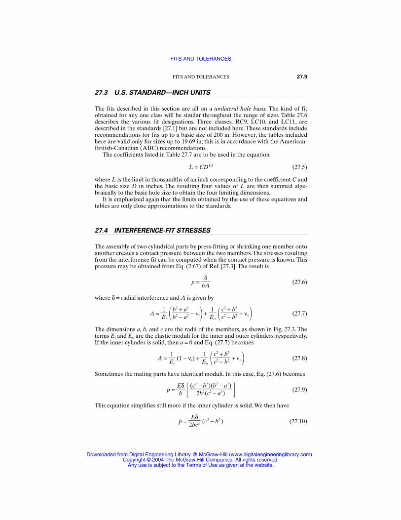
27.3 U.S. STANDARD—INCH UNITS
The fits described in this section are all on a unilateral hole basis. The kind of fitobtained for any one class will be similar throughout the range of sizes. Table 27.6describes the various fit designations. Three classes, RC9, LC10, and LC11, aredescribed in the standards [27.1] but are not included here. These standards includerecommendations for fits up to a basic size of 200 in. However, the tables includedhere are valid only for sizes up to 19.69 in; this is in accordance with the American-British-Canadian (ABC) recommendations.
The coefficients listed in Table 27.7 are to be used in the equation
L = CD1/3 (27.5)
where L is the limit in thousandths of an inch corresponding to the coefficient C andthe basic size D in inches. The resulting four values of L are then summed alge-braically to the basic hole size to obtain the four limiting dimensions.
It is emphasized again that the limits obtained by the use of these equations andtables are only close approximations to the standards.
27.4 INTERFERENCE-FIT STRESSES
The assembly of two cylindrical parts by press-fitting or shrinking one member ontoanother creates a contact pressure between the two members. The stresses resultingfrom the interference fit can be computed when the contact pressure is known. Thispressure may be obtained from Eq. (2.67) of Ref. [27.3]. The result is
p = bδA (27.6)
where δ = radial interference and A is given by
A = E1
i − νi +
E1
o + νo (27.7)
The dimensions a, b, and c are the radii of the members, as shown in Fig. 27.3. Theterms Ei and Eo are the elastic moduli for the inner and outer cylinders, respectively.If the inner cylinder is solid, then a = 0 and Eq. (27.7) becomes
A = E1
i (1 − νi) +
E1
o + νo (27.8)
Sometimes the mating parts have identical moduli. In this case, Eq. (27.6) becomes
p = Ebδ (27.9)
This equation simplifies still more if the inner cylinder is solid. We then have
p = (c2 − b2) (27.10)Eδ2bc2
(c2 − b2)(b2 − a2)
2b2(c2 − a2)
c2 + b2
c2 − b2
c2 + b2
c2 − b2
b2 + a2
b2 − a2
FITS AND TOLERANCES 27.9
FITS AND TOLERANCES
Downloaded from Digital Engineering Library @ McGraw-Hill (www.digitalengineeringlibrary.com)Copyright © 2004 The McGraw-Hill Companies. All rights reserved.
Any use is subject to the Terms of Use as given at the website.
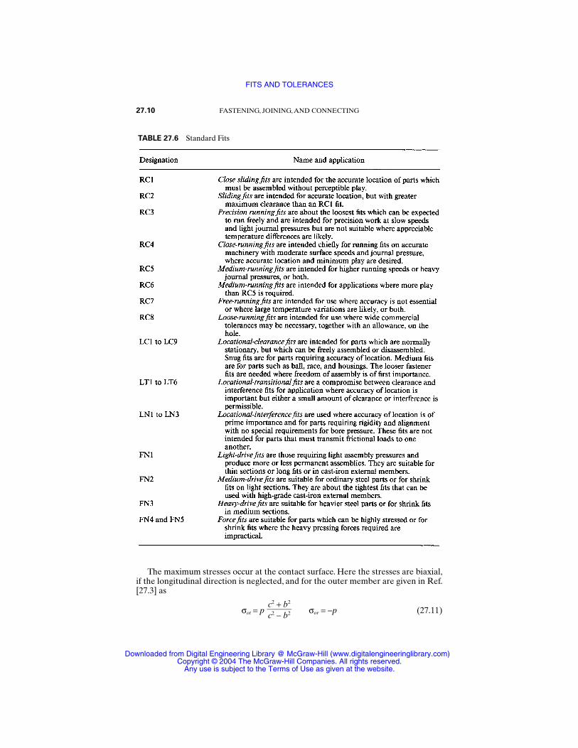
The maximum stresses occur at the contact surface. Here the stresses are biaxial,if the longitudinal direction is neglected, and for the outer member are given in Ref.[27.3] as
σot = p σor = −p (27.11)c2 + b2
c2 − b2
27.10 FASTENING, JOINING, AND CONNECTING
TABLE 27.6 Standard Fits
FITS AND TOLERANCES
Downloaded from Digital Engineering Library @ McGraw-Hill (www.digitalengineeringlibrary.com)Copyright © 2004 The McGraw-Hill Companies. All rights reserved.
Any use is subject to the Terms of Use as given at the website.
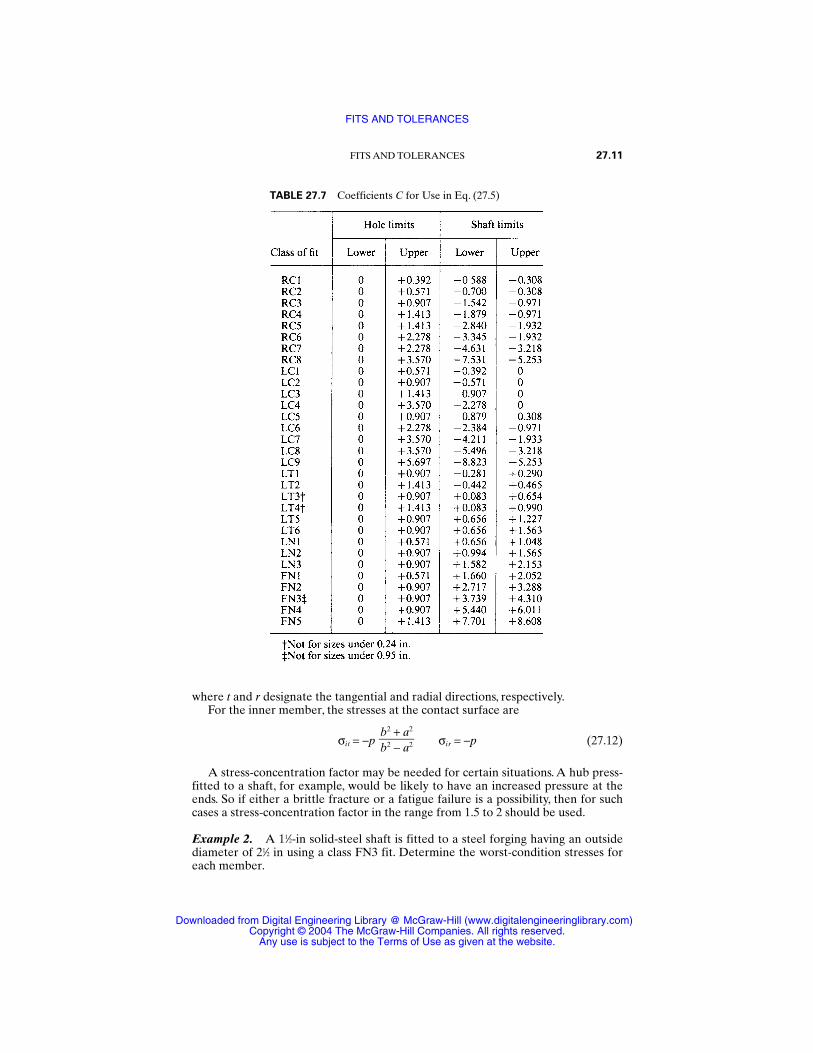
where t and r designate the tangential and radial directions, respectively.For the inner member, the stresses at the contact surface are
σit = −p σir = −p (27.12)
A stress-concentration factor may be needed for certain situations. A hub press-fitted to a shaft, for example, would be likely to have an increased pressure at theends. So if either a brittle fracture or a fatigue failure is a possibility, then for suchcases a stress-concentration factor in the range from 1.5 to 2 should be used.
Example 2. A 11⁄2-in solid-steel shaft is fitted to a steel forging having an outsidediameter of 21⁄2 in using a class FN3 fit. Determine the worst-condition stresses foreach member.
b2 + a2
b2 − a2
FITS AND TOLERANCES 27.11
TABLE 27.7 Coefficients C for Use in Eq. (27.5)
FITS AND TOLERANCES
Downloaded from Digital Engineering Library @ McGraw-Hill (www.digitalengineeringlibrary.com)Copyright © 2004 The McGraw-Hill Companies. All rights reserved.
Any use is subject to the Terms of Use as given at the website.
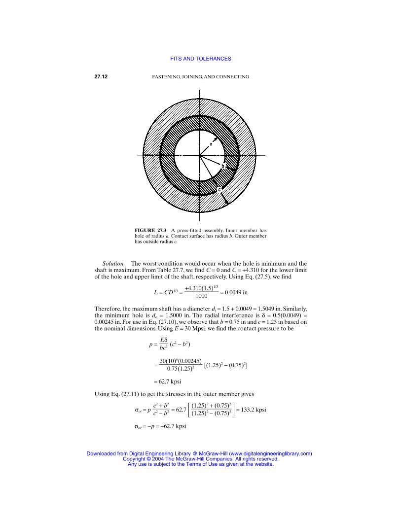
Solution. The worst condition would occur when the hole is minimum and theshaft is maximum. From Table 27.7, we find C = 0 and C = +4.310 for the lower limitof the hole and upper limit of the shaft, respectively. Using Eq. (27.5), we find
L = CD1/3 = = 0.0049 in
Therefore, the maximum shaft has a diameter di = 1.5 + 0.0049 = 1.5049 in. Similarly,the minimum hole is do = 1.5000 in. The radial interference is δ = 0.5(0.0049) =0.00245 in. For use in Eq. (27.10), we observe that b = 0.75 in and c = 1.25 in based onthe nominal dimensions. Using E = 30 Mpsi, we find the contact pressure to be
p = (c2 − b2)
= [(1.25)2 − (0.75)2]
= 62.7 kpsi
Using Eq. (27.11) to get the stresses in the outer member gives
σot = p = 62.7 = 133.2 kpsi
σor = −p = −62.7 kpsi
(1.25)2 + (0.75)2
(1.25)2 − (0.75)2
c2 + b2
c2 − b2
30(10)6(0.00245)
0.75(1.25)2
Eδbc2
+4.310(1.5)1/3
1000
27.12 FASTENING, JOINING, AND CONNECTING
FIGURE 27.3 A press-fitted assembly. Inner member hashole of radius a. Contact surface has radius b. Outer memberhas outside radius c.
FITS AND TOLERANCES
Downloaded from Digital Engineering Library @ McGraw-Hill (www.digitalengineeringlibrary.com)Copyright © 2004 The McGraw-Hill Companies. All rights reserved.
Any use is subject to the Terms of Use as given at the website.
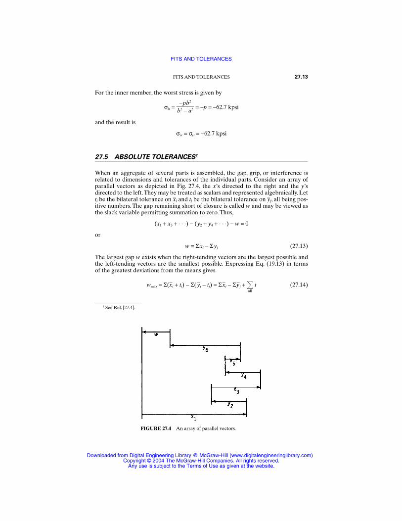
For the inner member, the worst stress is given by
σit = = −p = −62.7 kpsi
and the result is
σir = σit = −62.7 kpsi
27.5 ABSOLUTE TOLERANCES†
When an aggregate of several parts is assembled, the gap, grip, or interference isrelated to dimensions and tolerances of the individual parts. Consider an array ofparallel vectors as depicted in Fig. 27.4, the x’s directed to the right and the y’sdirected to the left.They may be treated as scalars and represented algebraically. Letti be the bilateral tolerance on xi and tj be the bilateral tolerance on yj, all being pos-itive numbers. The gap remaining short of closure is called w and may be viewed asthe slack variable permitting summation to zero. Thus,
(x1 + x3 + ⋅ ⋅ ⋅) − (y2 + y4 + ⋅ ⋅ ⋅) − w = 0
or
w = Σxi − Σyj (27.13)
The largest gap w exists when the right-tending vectors are the largest possible andthe left-tending vectors are the smallest possible. Expressing Eq. (19.13) in terms of the greatest deviations from the means gives
wmax = Σ(xi + ti) − Σ(yj − tj) = Σxi − Σyj + all
t (27.14)
−pb2
b2 − a2
FITS AND TOLERANCES 27.13
FIGURE 27.4 An array of parallel vectors.
† See Ref. [27.4].
FITS AND TOLERANCES
Downloaded from Digital Engineering Library @ McGraw-Hill (www.digitalengineeringlibrary.com)Copyright © 2004 The McGraw-Hill Companies. All rights reserved.
Any use is subject to the Terms of Use as given at the website.
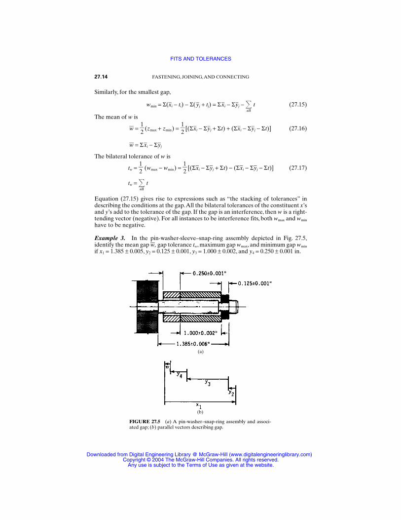
Similarly, for the smallest gap,
wmin = Σ(xi − ti) − Σ(yj + tj) = Σxi − Σyj − all
t (27.15)
The mean of w is
w = 12
(zmax + zmin) = 12
[(Σxi − Σyj + Σt) + (Σxi − Σyj − Σt)] (27.16)
w = Σxi − Σyj
The bilateral tolerance of w is
tw = 12
(wmax − wmin) = 12
[(Σxi − Σyj + Σt) − (Σxi − Σyj − Σt)] (27.17)
tw = all
t
Equation (27.15) gives rise to expressions such as “the stacking of tolerances” indescribing the conditions at the gap.All the bilateral tolerances of the constituent x’sand y’s add to the tolerance of the gap. If the gap is an interference, then w is a right-tending vector (negative). For all instances to be interference fits, both wmax and wmin
have to be negative.
Example 3. In the pin-washer-sleeve–snap-ring assembly depicted in Fig. 27.5,identify the mean gap w, gap tolerance tw, maximum gap wmax, and minimum gap wmin
if x1 = 1.385 ± 0.005, y2 = 0.125 ± 0.001, y3 = 1.000 ± 0.002, and y4 = 0.250 ± 0.001 in.
27.14 FASTENING, JOINING, AND CONNECTING
FIGURE 27.5 (a) A pin-washer–snap-ring assembly and associ-ated gap; (b) parallel vectors describing gap.
(a)
(b)
FITS AND TOLERANCES
Downloaded from Digital Engineering Library @ McGraw-Hill (www.digitalengineeringlibrary.com)Copyright © 2004 The McGraw-Hill Companies. All rights reserved.
Any use is subject to the Terms of Use as given at the website.
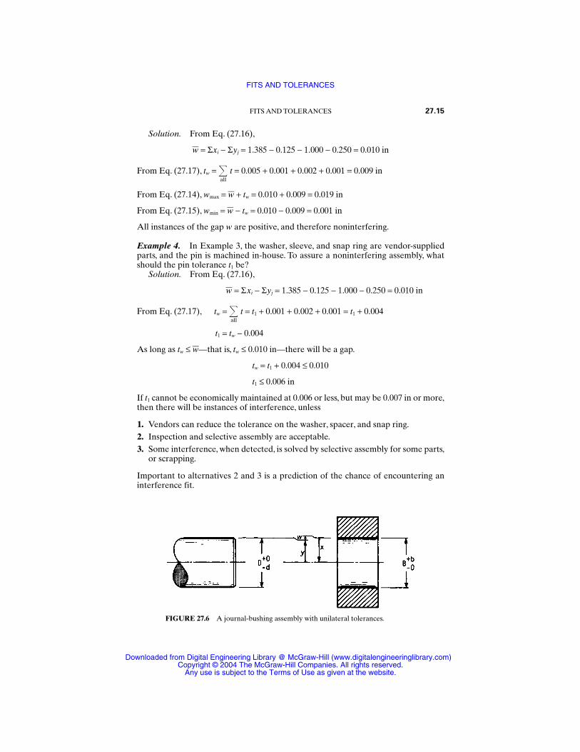
Solution. From Eq. (27.16),
w = Σxi − Σyj = 1.385 − 0.125 − 1.000 − 0.250 = 0.010 in
From Eq. (27.17), tw = all
t = 0.005 + 0.001 + 0.002 + 0.001 = 0.009 in
From Eq. (27.14), wmax = w + tw = 0.010 + 0.009 = 0.019 in
From Eq. (27.15), wmin = w − tw = 0.010 − 0.009 = 0.001 in
All instances of the gap w are positive, and therefore noninterfering.
Example 4. In Example 3, the washer, sleeve, and snap ring are vendor-suppliedparts, and the pin is machined in-house. To assure a noninterfering assembly, whatshould the pin tolerance t1 be?
Solution. From Eq. (27.16),
w = Σxi − Σyj = 1.385 − 0.125 − 1.000 − 0.250 = 0.010 in
From Eq. (27.17), tw = all
t = t1 + 0.001 + 0.002 + 0.001 = t1 + 0.004
t1 = tw − 0.004
As long as tw ≤ w—that is, tw ≤ 0.010 in—there will be a gap.
tw = t1 + 0.004 ≤ 0.010
t1 ≤ 0.006 in
If t1 cannot be economically maintained at 0.006 or less, but may be 0.007 in or more,then there will be instances of interference, unless
1. Vendors can reduce the tolerance on the washer, spacer, and snap ring.2. Inspection and selective assembly are acceptable.3. Some interference, when detected, is solved by selective assembly for some parts,
or scrapping.
Important to alternatives 2 and 3 is a prediction of the chance of encountering aninterference fit.
FITS AND TOLERANCES 27.15
FIGURE 27.6 A journal-bushing assembly with unilateral tolerances.
FITS AND TOLERANCES
Downloaded from Digital Engineering Library @ McGraw-Hill (www.digitalengineeringlibrary.com)Copyright © 2004 The McGraw-Hill Companies. All rights reserved.
Any use is subject to the Terms of Use as given at the website.
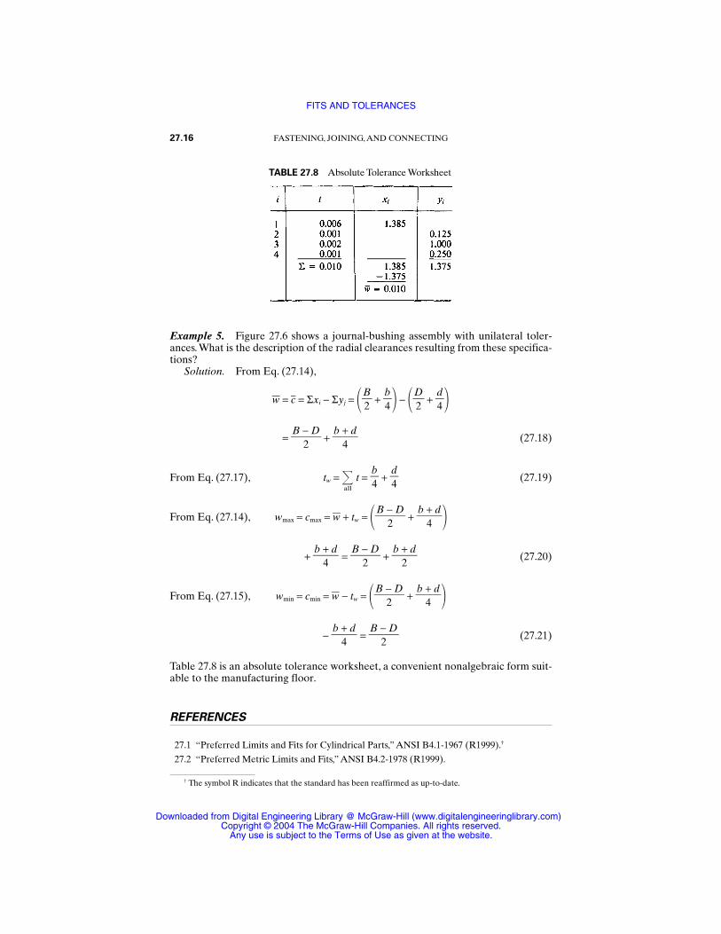
Example 5. Figure 27.6 shows a journal-bushing assembly with unilateral toler-ances.What is the description of the radial clearances resulting from these specifica-tions?
Solution. From Eq. (27.14),
w = c = Σxi − Σyj = B2
+ b4
− D2 +
d4
=
B −2
D +
b +4
d (27.18)
From Eq. (27.17), tw = all
t = b4
+ d4
(27.19)
From Eq. (27.14), wmax = cmax = w + tw = B −2
D +
b +4
d
+ b +
4d
= B −
2D
+ b +
2d
(27.20)
From Eq. (27.15), wmin = cmin = w − tw = B −2
D +
b +4
d
− b +
4d
= B −
2D
(27.21)
Table 27.8 is an absolute tolerance worksheet, a convenient nonalgebraic form suit-able to the manufacturing floor.
REFERENCES
27.1 “Preferred Limits and Fits for Cylindrical Parts,” ANSI B4.1-1967 (R1999).†
27.2 “Preferred Metric Limits and Fits,” ANSI B4.2-1978 (R1999).
27.16 FASTENING, JOINING, AND CONNECTING
TABLE 27.8 Absolute Tolerance Worksheet
† The symbol R indicates that the standard has been reaffirmed as up-to-date.
FITS AND TOLERANCES
Downloaded from Digital Engineering Library @ McGraw-Hill (www.digitalengineeringlibrary.com)Copyright © 2004 The McGraw-Hill Companies. All rights reserved.
Any use is subject to the Terms of Use as given at the website.

27.3 Joseph E. Shigley and Charles R. Mischke, Mechanical Engineering Design, 5th ed.,McGraw-Hill, New York, 1989.
27.4 M. F. Spotts, Dimensioning and Tolerancing for Quality Production, Prentice-Hall,Englewood Cliffs, N.J., 1983. (Excellent bibliography on standards and handbooks,dimensioning and tolerancing, quality control, gauging and shop practice, probabilityand statistics.)
FITS AND TOLERANCES 27.17
FITS AND TOLERANCES
Downloaded from Digital Engineering Library @ McGraw-Hill (www.digitalengineeringlibrary.com)Copyright © 2004 The McGraw-Hill Companies. All rights reserved.
Any use is subject to the Terms of Use as given at the website.

FITS AND TOLERANCES
Downloaded from Digital Engineering Library @ McGraw-Hill (www.digitalengineeringlibrary.com)Copyright © 2004 The McGraw-Hill Companies. All rights reserved.
Any use is subject to the Terms of Use as given at the website.

P • A • R • T • 7
LOAD CAPABILITYCONSIDERATIONS
Source: STANDARD HANDBOOK OF MACHINE DESIGN
Downloaded from Digital Engineering Library @ McGraw-Hill (www.digitalengineeringlibrary.com)Copyright © 2004 The McGraw-Hill Companies. All rights reserved.
Any use is subject to the Terms of Use as given at the website.

LOAD CAPABILITY CONSIDERATIONS
Downloaded from Digital Engineering Library @ McGraw-Hill (www.digitalengineeringlibrary.com)Copyright © 2004 The McGraw-Hill Companies. All rights reserved.
Any use is subject to the Terms of Use as given at the website.

CHAPTER 28STRENGTH UNDER STATIC
CIRCUMSTANCES
Charles R. Mischke, Ph.D., P.E.Professor Emeritus of Mechanical Engineering
Iowa State UniversityAmes, Iowa
Joseph E. ShigleyProfessor Emeritus
The University of MichiganAnn Arbor, Michigan
28.1 PERMISSIBLE STRESSES AND STRAINS / 28.4
28.2 THEORY OF STATIC FAILURE / 28.5
28.3 STRESS CONCENTRATION / 28.9
28.4 FRACTURE MECHANICS / 28.13
28.5 NONFERROUS METALS / 28.19
REFERENCES / 28.22
GLOSSARY OF SYMBOLS
a Crack semilengthA AreaD, d DiameterF Force or loadI Second moment of areaJ Second polar moment of areaK Stress-intensity factorK′ Stress-concentration factor for static loadingKc Critical-stress-intensity factorKt Normal-stress-concentration factorKts Shear-stress-concentration factorM Momentn Design factorqs Sensitivity index
28.3
Source: STANDARD HANDBOOK OF MACHINE DESIGN
Downloaded from Digital Engineering Library @ McGraw-Hill (www.digitalengineeringlibrary.com)Copyright © 2004 The McGraw-Hill Companies. All rights reserved.
Any use is subject to the Terms of Use as given at the website.
r Radius or ratioSsy Yield strength in shearSuc Ultimate compressive strengthSut Ultimate tensile strengthSy Yield strengthη Factor of safetyσ Normal stressσ′ von Mises stressτ Shear stressτo Octahedral shear stress or nominal shear stress
28.1 PERMISSIBLE STRESSES AND STRAINS
The discovery of the relationship between stress and strain during elastic and plasticdeformation allows interpretation either as a stress problem or as a strain problem.Imposed conditions on machine elements are more often loads than deformations,and so the usual focus is on stress rather than strain. Consequently, when durabilityunder static conditions is addressed, attention to permissible stress is more commonthan attention to permissible strain.
Permissible stress levels are established by
Experience with successful machine elements Laboratory simulations of field conditions Corporate experience manifested as a design-manual edict Codes, standards, and state of the art
During the design process, permissible stress levels are established by dividingthe significant strength by a design factor n. The design factor represents the originalintent or goal.As decisions involving discrete sizes are made, the stress levels departfrom those intended. The quotient, obtained by dividing the significant strength bythe load-induced stress at the critical location, is the factor of safety η, which isunique to the completed design.The design factor represents the goal and the factorof safety represents attainment.The adequacy assessment of a design includes exam-ination of the factor of safety. Finding a permissible stress level which will providesatisfactory service is not difficult. Competition forces a search for the highest stresslevel which still permits satisfactory service. This is more difficult.
Permissible stress level is a function of material strength, which is assessible onlyby test. Testing is costly. Where there is neither time nor money available or testingthe part is impossible, investigators have proposed theories of failure for guidance ofdesigners. Use of a theory of failure involves (1) identifying the significant stress atthe critical location and (2) comparing that stress condition with the strength of thepart at that location in the condition and geometry of use. Standardized tests, such asthe simple tension test, Jominy test, and others, provide some of the necessary infor-mation. For example, initiation of general yielding in a ductile part is predicted onthe basis of yield strength exhibited in the simple tension test and modified by themanufacturing process. Rupture of brittle parts is predicted on the basis of ultimatestrength (see Chap. 33).
28.4 LOAD CAPABILITY CONSIDERATIONS
STRENGTH UNDER STATIC CIRCUMSTANCES
Downloaded from Digital Engineering Library @ McGraw-Hill (www.digitalengineeringlibrary.com)Copyright © 2004 The McGraw-Hill Companies. All rights reserved.
Any use is subject to the Terms of Use as given at the website.
Estimates of permissible stress level for long and satisfactory performance offunction as listed above are based on design factors reflecting these experiences andare modified by the following:
1. Uncertainty as to material properties within a part, within a bar of steelstock, and within a heat of steel or whatever material is being considered for thedesign. Properties used by a designer may come not from an actual test, but from his-torical experience, since parts are sometimes designed before the material fromwhich they will be made has even been produced.
2. Uncertainty owing to the discrepancy between the designed part and the nec-essarily small size of the test specimen. The influence of size on strength is such thatsmaller parts tend to exhibit larger strengths.
3. Uncertainty concerning the actual effects of the manufacturing process onthe local material properties at the critical locations in the part. Processes such asupsetting, cold or hot forming, heat treatment, and surface treatment changestrengths and other properties.
4. Uncertainties as to the true effect of peripheral assembly operations onstrengths and other properties. Nearby weldments, mechanical fasteners, shrink fits,etc., all have influences that are difficult to predict with any precision.
5. Uncertainty as to the effect of elapsed time on properties.Aging in steels, alu-minums, and other alloys occurs, and some strengthening mechanisms are time-dependent. Corrosion is another time-dependent enemy of integrity.
6. Uncertainty as to the actual operating environment.7. Uncertainty as to the validity and precision of the mathematical models
employed in reaching decisions on the geometric specifications of a part.8. Uncertainty as to the intensity and dispersion of loads that may or will be
imposed on a machine member and as to the understanding of the effect of impact.9. Uncertainty as to the stress concentrations actually present in a manufac-
tured part picked at random for assembly and use. Changes in tool radius due towear, regrinding, or replacement can have a significant influence on the stress levelsactually attained in parts in service.
10. Company design policies or the dictates of codes.11. Uncertainty as to the completeness of a list of uncertainties.
Although specific recommendations that suggest design factors qualified byusage are to be found in many places, such factors depend on the stochastic natureof properties, loading, geometry, the form of functional relationships between them,and the reliability goal.
28.2 THEORY OF STATIC FAILURE
For ductile materials, the best estimation method for predicting the onset of yielding,for materials exhibiting equal strengths in tension and compression, is the octahe-dral shear theory (distortion energy or Hencky-von Mises). The octahedral shearstress is
τo = 1⁄3[(σ1 − σ2)2 + (σ2 − σ3)2 + (σ3 − σ1)2]1/2
STRENGTH UNDER STATIC CIRCUMSTANCES 28.5
STRENGTH UNDER STATIC CIRCUMSTANCES
Downloaded from Digital Engineering Library @ McGraw-Hill (www.digitalengineeringlibrary.com)Copyright © 2004 The McGraw-Hill Companies. All rights reserved.
Any use is subject to the Terms of Use as given at the website.
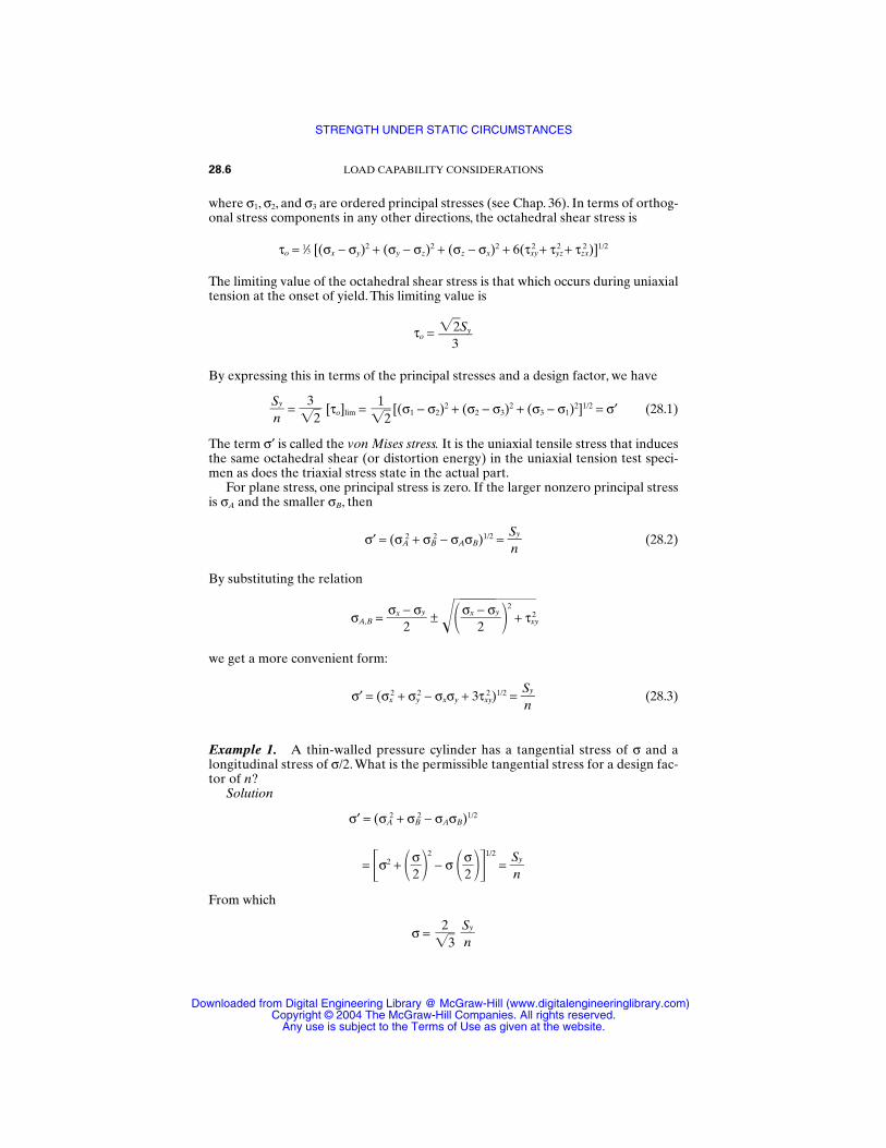
where σ1, σ2, and σ3 are ordered principal stresses (see Chap. 36). In terms of orthog-onal stress components in any other directions, the octahedral shear stress is
τo = 1⁄3 [(σx − σy)2 + (σy − σz)2 + (σz − σx)2 + 6(τxy2 + τyz
2 + τzx2 )]1/2
The limiting value of the octahedral shear stress is that which occurs during uniaxialtension at the onset of yield. This limiting value is
τo =
By expressing this in terms of the principal stresses and a design factor, we have
= [τo]lim = [(σ1 − σ2)2 + (σ2 − σ3)2 + (σ3 − σ1)2]1/2 = σ′ (28.1)
The term σ′ is called the von Mises stress. It is the uniaxial tensile stress that inducesthe same octahedral shear (or distortion energy) in the uniaxial tension test speci-men as does the triaxial stress state in the actual part.
For plane stress, one principal stress is zero. If the larger nonzero principal stressis σA and the smaller σB, then
σ′ = (σA2 + σB
2 − σAσB)1/2 = (28.2)
By substituting the relation
σA,B = ± 2
+ τ xy2
we get a more convenient form:
σ′ = (σx2 + σy
2 − σxσy + 3τxy2)1/2 = (28.3)
Example 1. A thin-walled pressure cylinder has a tangential stress of σ and alongitudinal stress of σ/2. What is the permissible tangential stress for a design fac-tor of n?
Solution
σ′ = (σA2 + σB
2 − σAσB)1/2
= σ2 + σ2
2
− σ σ2
1/2
=
From which
σ = Syn
23
Syn
Syn
σx − σy
2σx − σy
2
Syn
12
32
Syn
2Sy3
28.6 LOAD CAPABILITY CONSIDERATIONS
STRENGTH UNDER STATIC CIRCUMSTANCES
Downloaded from Digital Engineering Library @ McGraw-Hill (www.digitalengineeringlibrary.com)Copyright © 2004 The McGraw-Hill Companies. All rights reserved.
Any use is subject to the Terms of Use as given at the website.
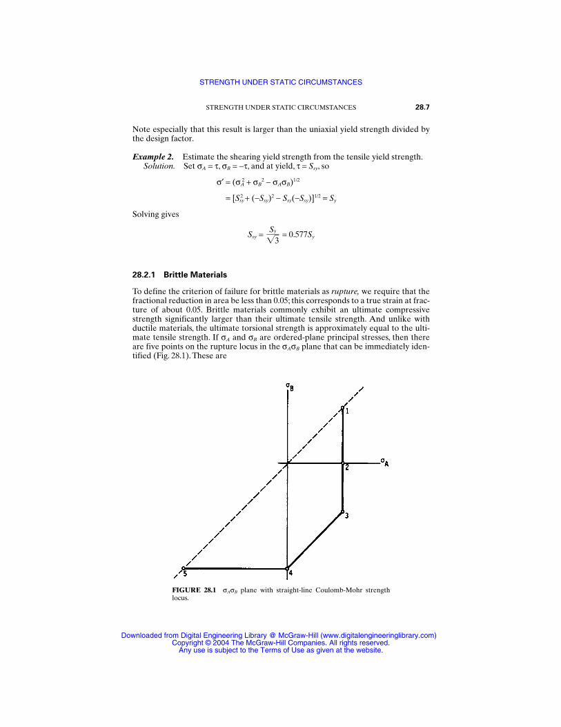
Note especially that this result is larger than the uniaxial yield strength divided bythe design factor.
Example 2. Estimate the shearing yield strength from the tensile yield strength.Solution. Set σA = τ, σB = −τ, and at yield, τ = Ssy, so
σ′ = (σA2 + σB
2 − σAσB)1/2
= [Ssy2 + (−Ssy)2 − Ssy(−Ssy)]1/2 = Sy
Solving gives
Ssy = = 0.577Sy
28.2.1 Brittle Materials
To define the criterion of failure for brittle materials as rupture, we require that thefractional reduction in area be less than 0.05; this corresponds to a true strain at frac-ture of about 0.05. Brittle materials commonly exhibit an ultimate compressivestrength significantly larger than their ultimate tensile strength. And unlike withductile materials, the ultimate torsional strength is approximately equal to the ulti-mate tensile strength. If σA and σB are ordered-plane principal stresses, then thereare five points on the rupture locus in the σAσB plane that can be immediately iden-tified (Fig. 28.1). These are
Sy3
STRENGTH UNDER STATIC CIRCUMSTANCES 28.7
FIGURE 28.1 σAσB plane with straight-line Coulomb-Mohr strengthlocus.
STRENGTH UNDER STATIC CIRCUMSTANCES
Downloaded from Digital Engineering Library @ McGraw-Hill (www.digitalengineeringlibrary.com)Copyright © 2004 The McGraw-Hill Companies. All rights reserved.
Any use is subject to the Terms of Use as given at the website.
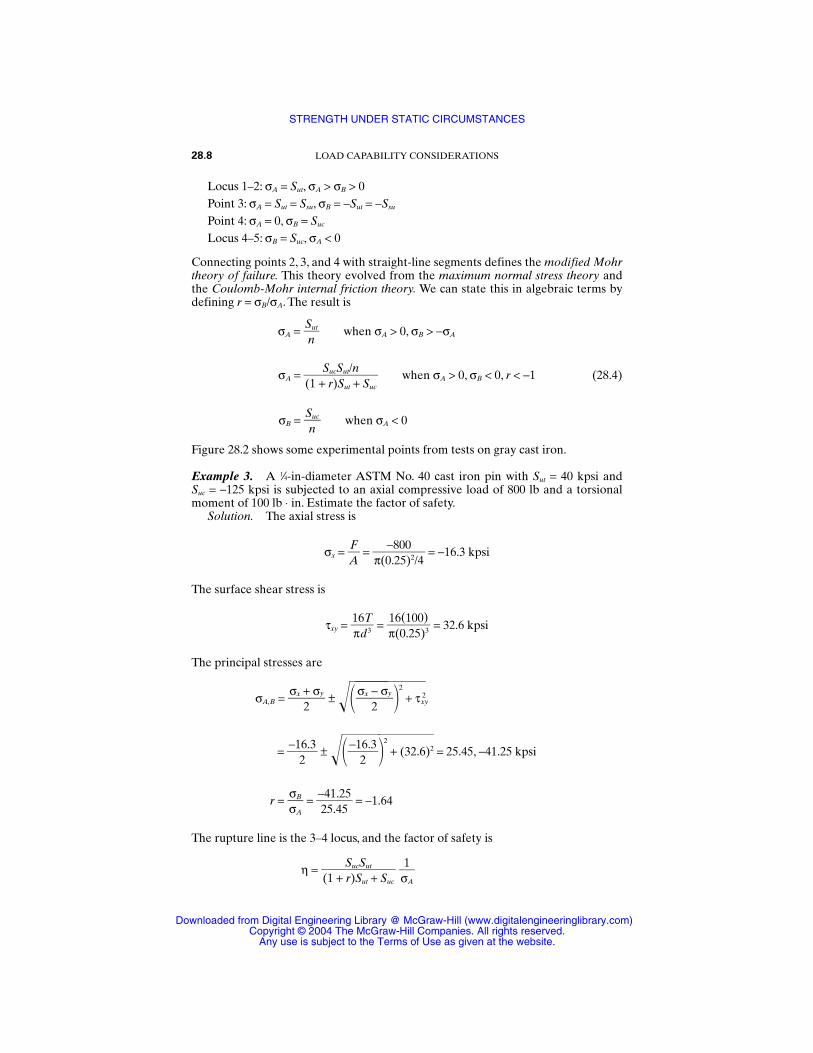
Locus 1–2: σA = Sut, σA > σB > 0Point 3: σA = Sut = Ssu, σB = −Sut = −Ssu
Point 4: σA = 0, σB = Suc
Locus 4–5: σB = Suc, σA < 0
Connecting points 2, 3, and 4 with straight-line segments defines the modified Mohrtheory of failure. This theory evolved from the maximum normal stress theory andthe Coulomb-Mohr internal friction theory. We can state this in algebraic terms bydefining r = σB/σA. The result is
σA = when σA > 0, σB > −σA
σA =(1 +
Sru
)cSS
u
u
t
t
/n+ Suc
when σA > 0, σB < 0, r < −1 (28.4)
σB = when σA < 0
Figure 28.2 shows some experimental points from tests on gray cast iron.
Example 3. A 1⁄4-in-diameter ASTM No. 40 cast iron pin with Sut = 40 kpsi and Suc = −125 kpsi is subjected to an axial compressive load of 800 lb and a torsionalmoment of 100 lb ⋅ in. Estimate the factor of safety.
Solution. The axial stress is
σx = AF
= π(0
−.82050)2/4
= −16.3 kpsi
The surface shear stress is
τxy = = = 32.6 kpsi
The principal stresses are
σA,B = ± 2
+ τ xy2
= −1
26.3 ± −1
26.3
2
+ ( 3 2 .6 )2 = 25.45, −41.25 kpsi
r = = −2451.4.255
= −1.64
The rupture line is the 3–4 locus, and the factor of safety is
η = σ1
A
SucSut(1 + r)Sut + Suc
σBσA
σx − σy
2σx + σy
2
16(100)π(0.25)3
16Tπd3
Sucn
Sutn
28.8 LOAD CAPABILITY CONSIDERATIONS
STRENGTH UNDER STATIC CIRCUMSTANCES
Downloaded from Digital Engineering Library @ McGraw-Hill (www.digitalengineeringlibrary.com)Copyright © 2004 The McGraw-Hill Companies. All rights reserved.
Any use is subject to the Terms of Use as given at the website.
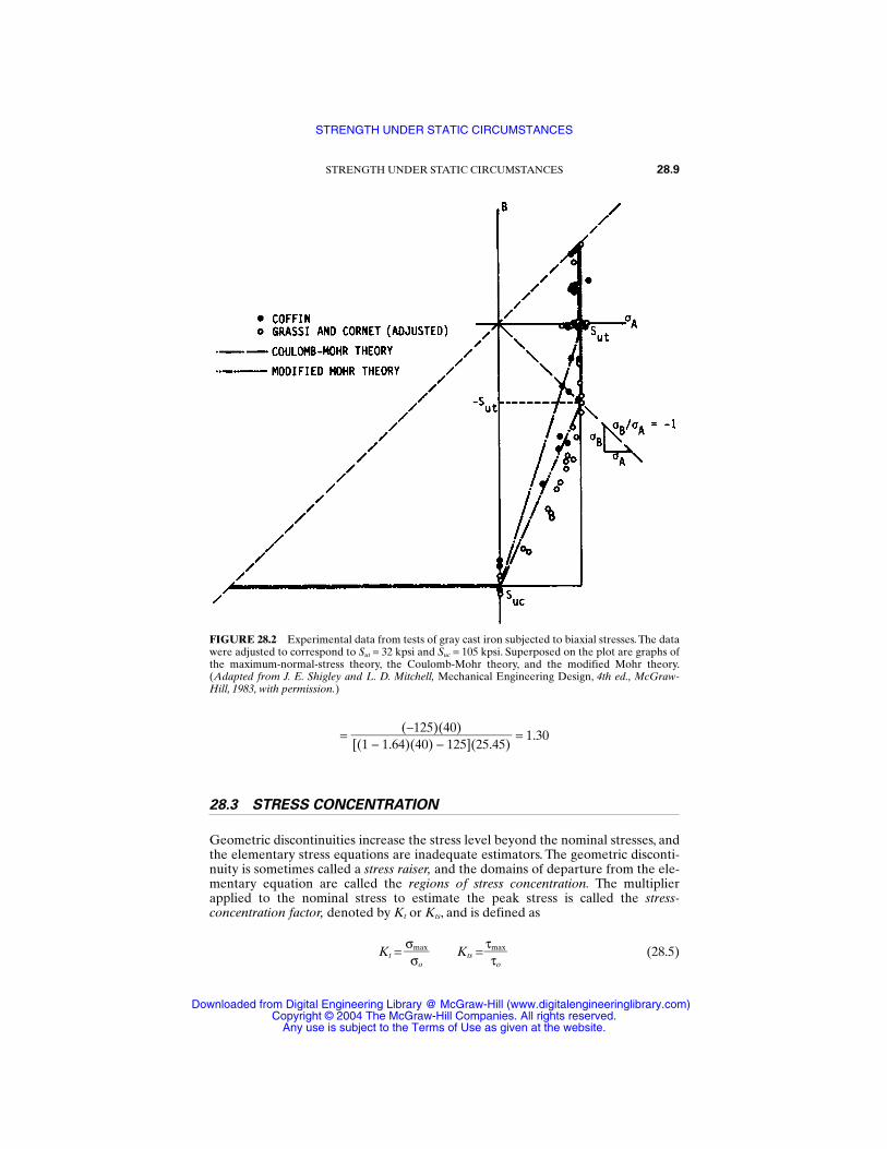
= = 1.30
28.3 STRESS CONCENTRATION
Geometric discontinuities increase the stress level beyond the nominal stresses, andthe elementary stress equations are inadequate estimators. The geometric disconti-nuity is sometimes called a stress raiser, and the domains of departure from the ele-mentary equation are called the regions of stress concentration. The multiplierapplied to the nominal stress to estimate the peak stress is called the stress-concentration factor, denoted by Kt or Kts, and is defined as
Kt = Kts = (28.5)τmaxτo
σmaxσo
(−125)(40)[(1 − 1.64)(40) − 125](25.45)
STRENGTH UNDER STATIC CIRCUMSTANCES 28.9
FIGURE 28.2 Experimental data from tests of gray cast iron subjected to biaxial stresses. The datawere adjusted to correspond to Sut = 32 kpsi and Suc = 105 kpsi. Superposed on the plot are graphs ofthe maximum-normal-stress theory, the Coulomb-Mohr theory, and the modified Mohr theory.(Adapted from J. E. Shigley and L. D. Mitchell, Mechanical Engineering Design, 4th ed., McGraw-Hill, 1983, with permission.)
STRENGTH UNDER STATIC CIRCUMSTANCES
Downloaded from Digital Engineering Library @ McGraw-Hill (www.digitalengineeringlibrary.com)Copyright © 2004 The McGraw-Hill Companies. All rights reserved.
Any use is subject to the Terms of Use as given at the website.

respectively. These factors depend solely on part geometry and manner of loadingand are independent of the material. Methods for determining stress-concentrationfactors include theory of elasticity, photoelasticity, numerical methods including finiteelements, gridding, brittle lacquers, brittle models, and strain-gauging techniques.
Peterson [28.1] has been responsible for many useful charts. Some charts repre-senting common geometries and loadings are included as Figs. 28.3 through 28.17.The user of any such charts is cautioned to use the nominal stress equation uponwhich the chart is based.
When the region of stress concentration is small compared to the section resist-ing the static loading, localized yielding in ductile materials limits the peak stress tothe approximate level of the yield strength. The load is carried without gross plasticdistortion. The stress concentration does no damage (strain strengthening occurs),and it can be ignored. No stress-concentration factor is applied to the stress. For low-ductility materials, such as the heat-treated and case-hardened steels, the full geo-metric stress-concentration factor is applied unless notch-sensitivity information tothe contrary is available. This notch-sensitivity equation is
K′ = 1 + qs(Kt − 1) (28.6)
where K′ = the actual stress-concentration factor for static loading and qs = an indexof sensitivity of the material in static loading determined by test. The value of qs forhardened steels is approximately 0.15 (if untempered, 0.25). For cast irons, whichhave internal discontinuities as severe as the notch, qs approaches zero and the fullvalue of Kt is rarely applied.
Kurajian and West [28.3] have derived stress-concentration factors for hollowstepped shafts. They develop an equivalent solid stepped shaft and then use theusual charts (Figs. 28.10 and 28.11) to find Kt. The formulas are
28.10 LOAD CAPABILITY CONSIDERATIONS
FIGURE 28.3 Bar in tension or simple compression with a transverse hole. σo = F/A, whereA = (w − d)t, and t = thickness. (From Peterson [28.2].)
STRENGTH UNDER STATIC CIRCUMSTANCES
Downloaded from Digital Engineering Library @ McGraw-Hill (www.digitalengineeringlibrary.com)Copyright © 2004 The McGraw-Hill Companies. All rights reserved.
Any use is subject to the Terms of Use as given at the website.
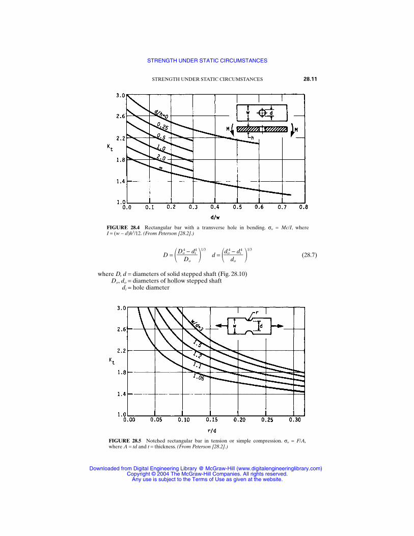
STRENGTH UNDER STATIC CIRCUMSTANCES 28.11
FIGURE 28.4 Rectangular bar with a transverse hole in bending. σo = Mc/I, whereI = (w − d)h3/12. (From Peterson [28.2].)
FIGURE 28.5 Notched rectangular bar in tension or simple compression. σo = F/A,where A = td and t = thickness. (From Peterson [28.2].)
D = 1/3
d = 1/3
(28.7)
where D, d = diameters of solid stepped shaft (Fig. 28.10)Do, do = diameters of hollow stepped shaft
di = hole diameter
do4 − di
4
do
Do4 − di
4
Do
STRENGTH UNDER STATIC CIRCUMSTANCES
Downloaded from Digital Engineering Library @ McGraw-Hill (www.digitalengineeringlibrary.com)Copyright © 2004 The McGraw-Hill Companies. All rights reserved.
Any use is subject to the Terms of Use as given at the website.
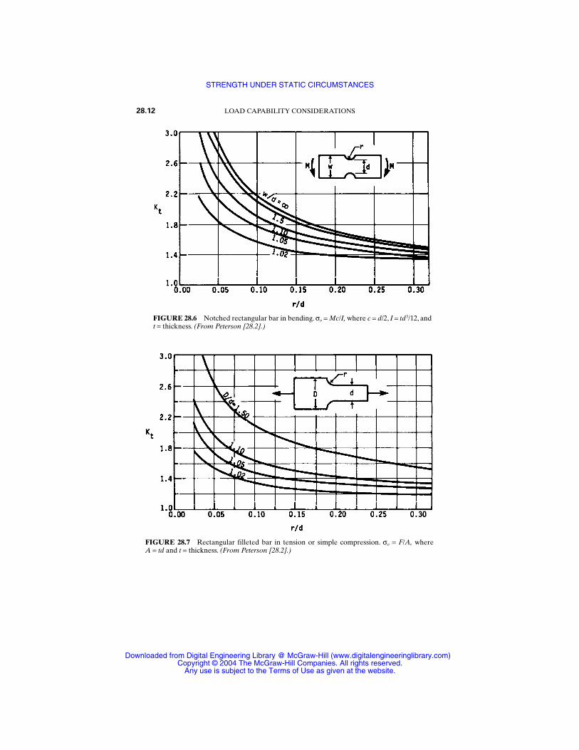
28.12 LOAD CAPABILITY CONSIDERATIONS
FIGURE 28.6 Notched rectangular bar in bending. σo = Mc/I, where c = d/2, I = td3/12, andt = thickness. (From Peterson [28.2].)
FIGURE 28.7 Rectangular filleted bar in tension or simple compression. σo = F/A, whereA = td and t = thickness. (From Peterson [28.2].)
STRENGTH UNDER STATIC CIRCUMSTANCES
Downloaded from Digital Engineering Library @ McGraw-Hill (www.digitalengineeringlibrary.com)Copyright © 2004 The McGraw-Hill Companies. All rights reserved.
Any use is subject to the Terms of Use as given at the website.
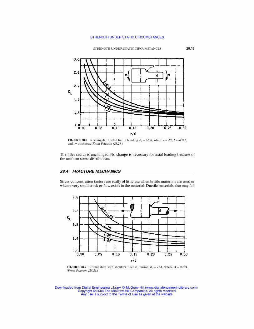
The fillet radius is unchanged. No change is necessary for axial loading because ofthe uniform stress distribution.
28.4 FRACTURE MECHANICS
Stress-concentration factors are really of little use when brittle materials are used orwhen a very small crack or flaw exists in the material. Ductile materials also may fail
STRENGTH UNDER STATIC CIRCUMSTANCES 28.13
FIGURE 28.8 Rectangular filleted bar in bending. σo = Mc/I, where c = d/2, I = td3/12,and t = thickness. (From Peterson [28.2].)
FIGURE 28.9 Round shaft with shoulder fillet in tension. σo = F/A, where A = πd2/4.(From Peterson [28.2].)
STRENGTH UNDER STATIC CIRCUMSTANCES
Downloaded from Digital Engineering Library @ McGraw-Hill (www.digitalengineeringlibrary.com)Copyright © 2004 The McGraw-Hill Companies. All rights reserved.
Any use is subject to the Terms of Use as given at the website.
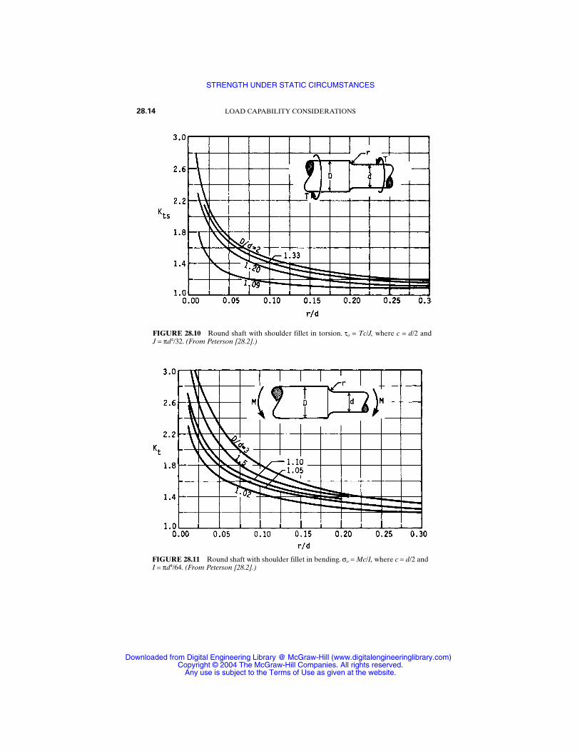
28.14 LOAD CAPABILITY CONSIDERATIONS
FIGURE 28.10 Round shaft with shoulder fillet in torsion. τo = Tc/J, where c = d/2 and J = πd4/32. (From Peterson [28.2].)
FIGURE 28.11 Round shaft with shoulder fillet in bending. σo = Mc/I, where c = d/2 andI = πd4/64. (From Peterson [28.2].)
STRENGTH UNDER STATIC CIRCUMSTANCES
Downloaded from Digital Engineering Library @ McGraw-Hill (www.digitalengineeringlibrary.com)Copyright © 2004 The McGraw-Hill Companies. All rights reserved.
Any use is subject to the Terms of Use as given at the website.
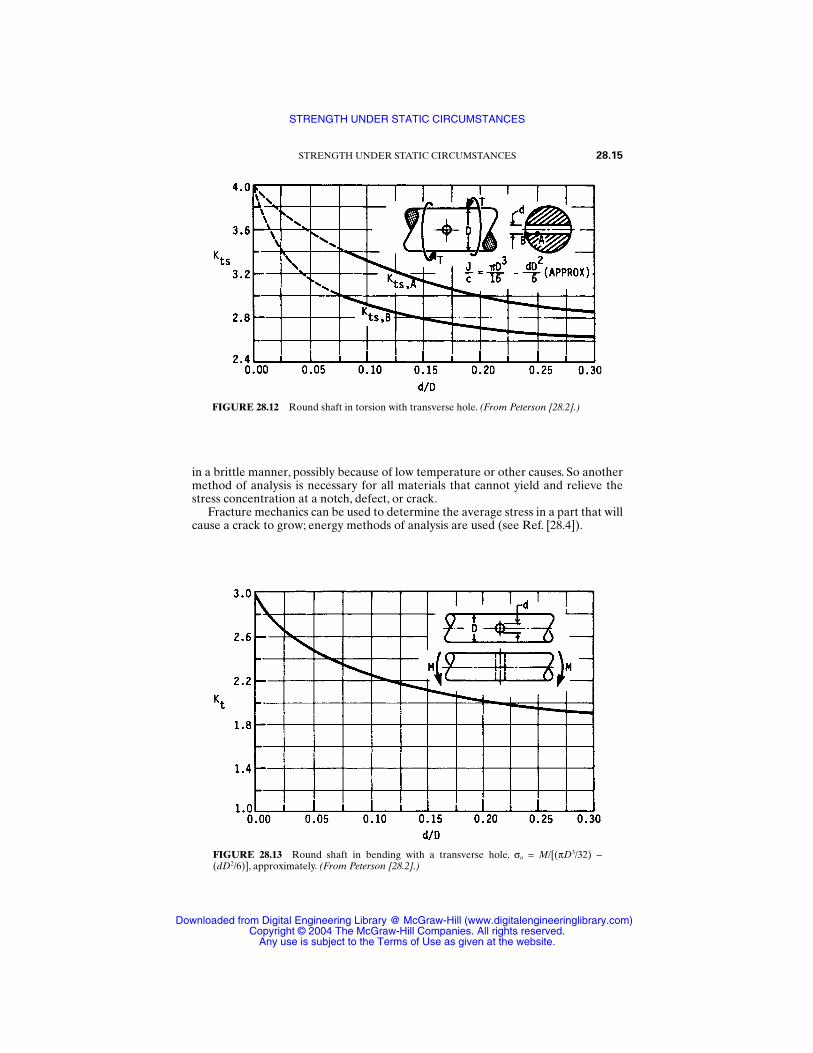
in a brittle manner, possibly because of low temperature or other causes. So anothermethod of analysis is necessary for all materials that cannot yield and relieve thestress concentration at a notch, defect, or crack.
Fracture mechanics can be used to determine the average stress in a part that willcause a crack to grow; energy methods of analysis are used (see Ref. [28.4]).
STRENGTH UNDER STATIC CIRCUMSTANCES 28.15
FIGURE 28.12 Round shaft in torsion with transverse hole. (From Peterson [28.2].)
FIGURE 28.13 Round shaft in bending with a transverse hole. σo = M/[(πD3/32) −(dD2/6)], approximately. (From Peterson [28.2].)
STRENGTH UNDER STATIC CIRCUMSTANCES
Downloaded from Digital Engineering Library @ McGraw-Hill (www.digitalengineeringlibrary.com)Copyright © 2004 The McGraw-Hill Companies. All rights reserved.
Any use is subject to the Terms of Use as given at the website.
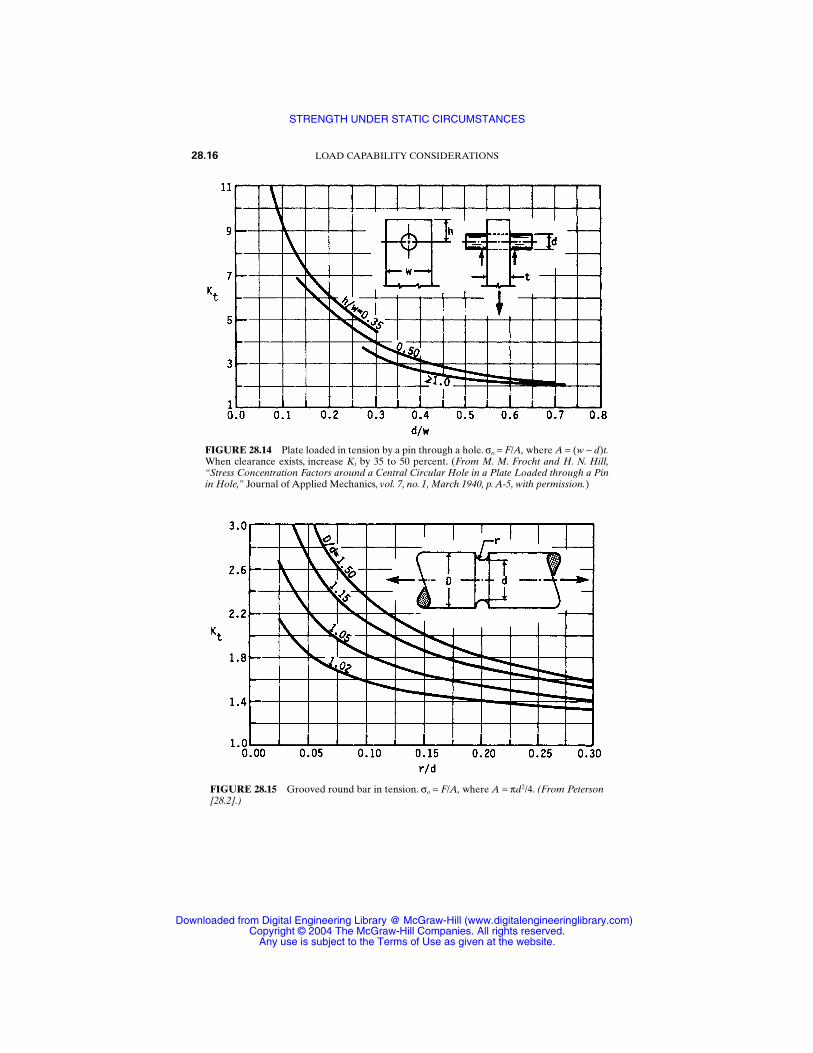
28.16 LOAD CAPABILITY CONSIDERATIONS
FIGURE 28.14 Plate loaded in tension by a pin through a hole. σo = F/A, where A = (w − d)t.When clearance exists, increase Kt by 35 to 50 percent. (From M. M. Frocht and H. N. Hill,“Stress Concentration Factors around a Central Circular Hole in a Plate Loaded through a Pinin Hole,” Journal of Applied Mechanics, vol. 7, no. 1, March 1940, p. A-5, with permission.)
FIGURE 28.15 Grooved round bar in tension. σo = F/A, where A = πd2/4. (From Peterson[28.2].)
STRENGTH UNDER STATIC CIRCUMSTANCES
Downloaded from Digital Engineering Library @ McGraw-Hill (www.digitalengineeringlibrary.com)Copyright © 2004 The McGraw-Hill Companies. All rights reserved.
Any use is subject to the Terms of Use as given at the website.
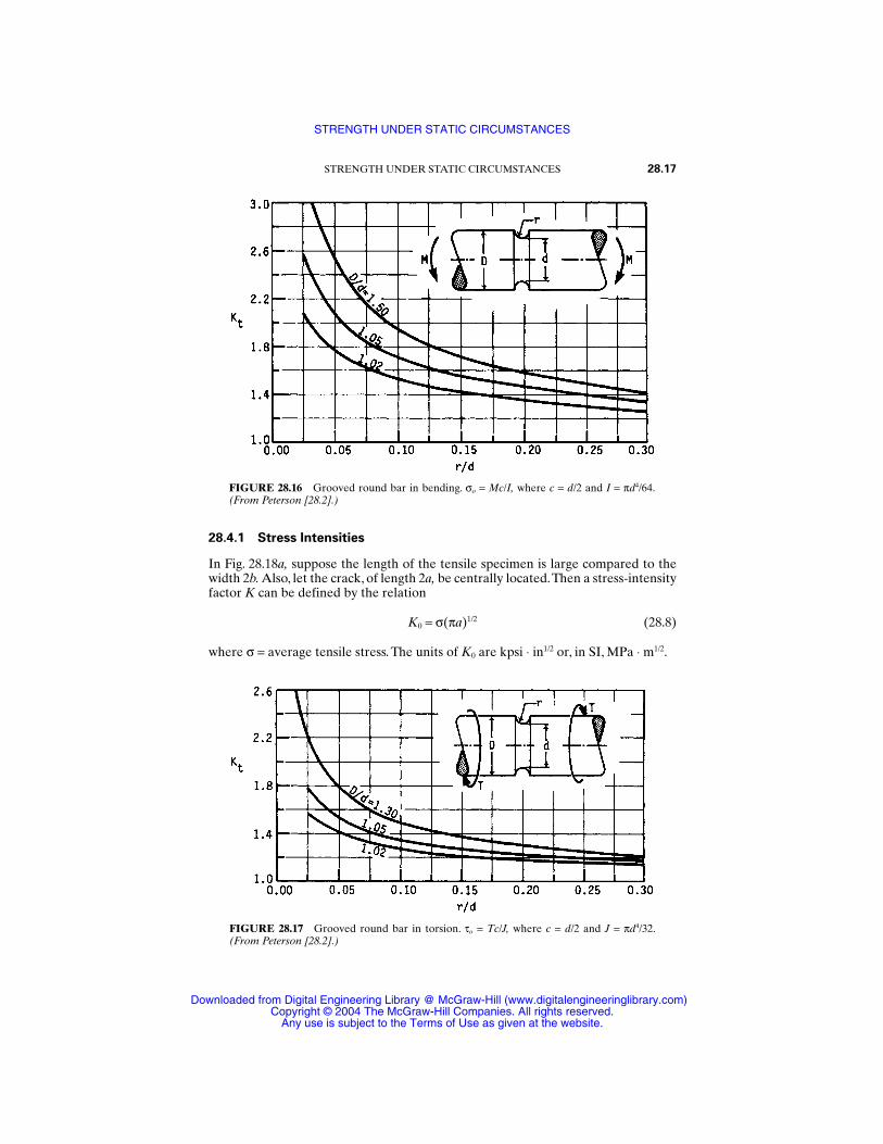
28.4.1 Stress Intensities
In Fig. 28.18a, suppose the length of the tensile specimen is large compared to thewidth 2b. Also, let the crack, of length 2a, be centrally located.Then a stress-intensityfactor K can be defined by the relation
K0 = σ(πa)1/2 (28.8)
where σ = average tensile stress. The units of K0 are kpsi ⋅ in1/2 or, in SI, MPa ⋅ m1/2.
STRENGTH UNDER STATIC CIRCUMSTANCES 28.17
FIGURE 28.16 Grooved round bar in bending. σo = Mc/I, where c = d/2 and I = πd4/64.(From Peterson [28.2].)
FIGURE 28.17 Grooved round bar in torsion. τo = Tc/J, where c = d/2 and J = πd4/32.(From Peterson [28.2].)
STRENGTH UNDER STATIC CIRCUMSTANCES
Downloaded from Digital Engineering Library @ McGraw-Hill (www.digitalengineeringlibrary.com)Copyright © 2004 The McGraw-Hill Companies. All rights reserved.
Any use is subject to the Terms of Use as given at the website.
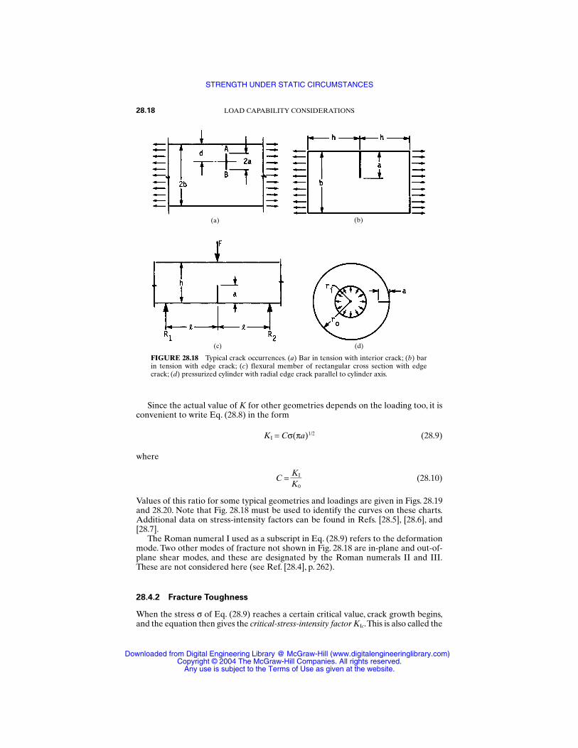
Since the actual value of K for other geometries depends on the loading too, it isconvenient to write Eq. (28.8) in the form
KI = Cσ(πa)1/2 (28.9)
where
C = (28.10)
Values of this ratio for some typical geometries and loadings are given in Figs. 28.19and 28.20. Note that Fig. 28.18 must be used to identify the curves on these charts.Additional data on stress-intensity factors can be found in Refs. [28.5], [28.6], and[28.7].
The Roman numeral I used as a subscript in Eq. (28.9) refers to the deformationmode. Two other modes of fracture not shown in Fig. 28.18 are in-plane and out-of-plane shear modes, and these are designated by the Roman numerals II and III.These are not considered here (see Ref. [28.4], p. 262).
28.4.2 Fracture Toughness
When the stress σ of Eq. (28.9) reaches a certain critical value, crack growth begins,and the equation then gives the critical-stress-intensity factor KIc.This is also called the
KIK0
28.18 LOAD CAPABILITY CONSIDERATIONS
FIGURE 28.18 Typical crack occurrences. (a) Bar in tension with interior crack; (b) barin tension with edge crack; (c) flexural member of rectangular cross section with edgecrack; (d) pressurized cylinder with radial edge crack parallel to cylinder axis.
(a) (b)
(c) (d)
STRENGTH UNDER STATIC CIRCUMSTANCES
Downloaded from Digital Engineering Library @ McGraw-Hill (www.digitalengineeringlibrary.com)Copyright © 2004 The McGraw-Hill Companies. All rights reserved.
Any use is subject to the Terms of Use as given at the website.
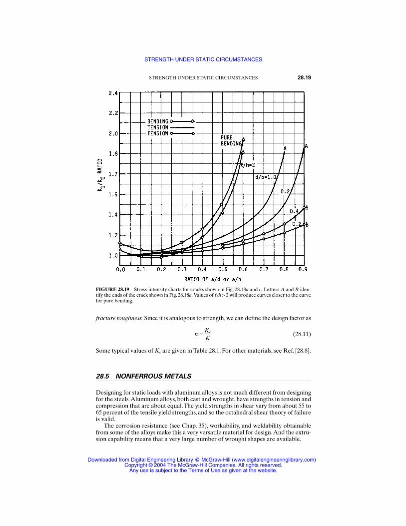
fracture toughness. Since it is analogous to strength, we can define the design factor as
n = (28.11)
Some typical values of Kc are given in Table 28.1. For other materials, see Ref. [28.8].
28.5 NONFERROUS METALS
Designing for static loads with aluminum alloys is not much different from designingfor the steels.Aluminum alloys, both cast and wrought, have strengths in tension andcompression that are about equal.The yield strengths in shear vary from about 55 to65 percent of the tensile yield strengths, and so the octahedral shear theory of failureis valid.
The corrosion resistance (see Chap. 35), workability, and weldability obtainablefrom some of the alloys make this a very versatile material for design.And the extru-sion capability means that a very large number of wrought shapes are available.
KcK
STRENGTH UNDER STATIC CIRCUMSTANCES 28.19
FIGURE 28.19 Stress-intensity charts for cracks shown in Fig. 28.18a and c. Letters A and B iden-tify the ends of the crack shown in Fig. 28.18a. Values of /h > 2 will produce curves closer to the curvefor pure bending.
STRENGTH UNDER STATIC CIRCUMSTANCES
Downloaded from Digital Engineering Library @ McGraw-Hill (www.digitalengineeringlibrary.com)Copyright © 2004 The McGraw-Hill Companies. All rights reserved.
Any use is subject to the Terms of Use as given at the website.
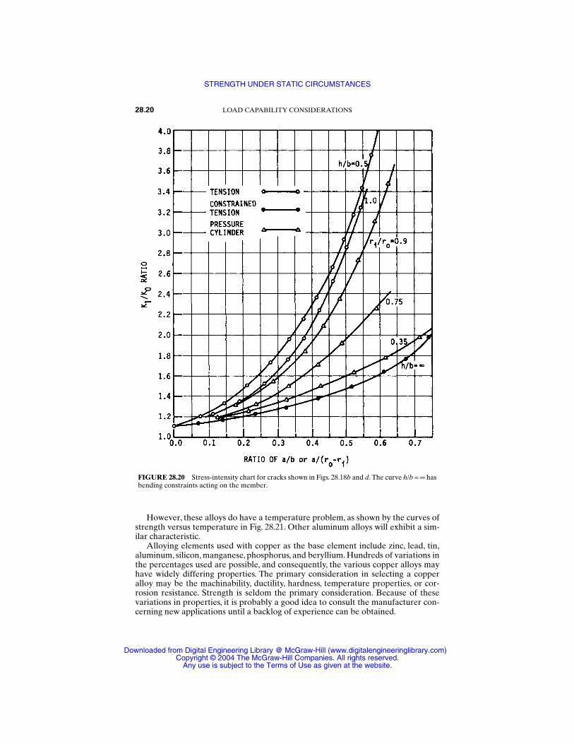
However, these alloys do have a temperature problem, as shown by the curves ofstrength versus temperature in Fig. 28.21. Other aluminum alloys will exhibit a sim-ilar characteristic.
Alloying elements used with copper as the base element include zinc, lead, tin,aluminum, silicon, manganese, phosphorus, and beryllium. Hundreds of variations inthe percentages used are possible, and consequently, the various copper alloys mayhave widely differing properties. The primary consideration in selecting a copperalloy may be the machinability, ductility, hardness, temperature properties, or cor-rosion resistance. Strength is seldom the primary consideration. Because of thesevariations in properties, it is probably a good idea to consult the manufacturer con-cerning new applications until a backlog of experience can be obtained.
28.20 LOAD CAPABILITY CONSIDERATIONS
FIGURE 28.20 Stress-intensity chart for cracks shown in Figs. 28.18b and d. The curve h/b = ∞ hasbending constraints acting on the member.
STRENGTH UNDER STATIC CIRCUMSTANCES
Downloaded from Digital Engineering Library @ McGraw-Hill (www.digitalengineeringlibrary.com)Copyright © 2004 The McGraw-Hill Companies. All rights reserved.
Any use is subject to the Terms of Use as given at the website.
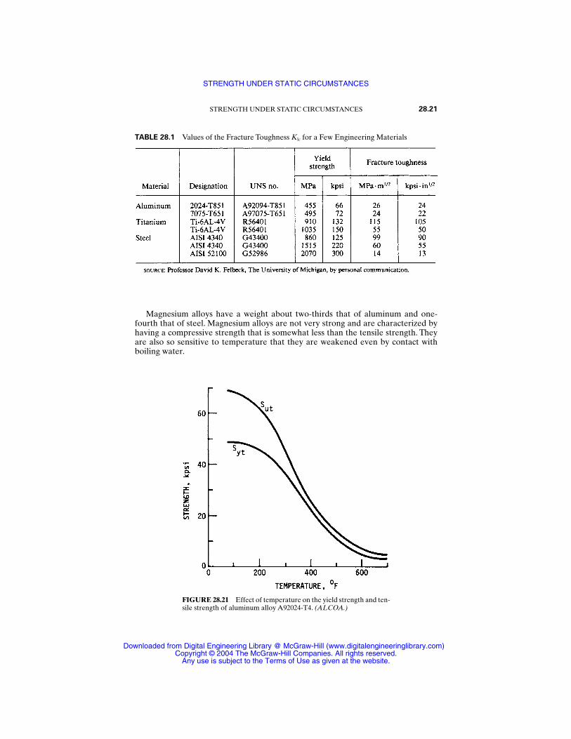
Magnesium alloys have a weight about two-thirds that of aluminum and one-fourth that of steel. Magnesium alloys are not very strong and are characterized byhaving a compressive strength that is somewhat less than the tensile strength. Theyare also so sensitive to temperature that they are weakened even by contact withboiling water.
STRENGTH UNDER STATIC CIRCUMSTANCES 28.21
TABLE 28.1 Values of the Fracture Toughness Klc for a Few Engineering Materials
FIGURE 28.21 Effect of temperature on the yield strength and ten-sile strength of aluminum alloy A92024-T4. (ALCOA.)
STRENGTH UNDER STATIC CIRCUMSTANCES
Downloaded from Digital Engineering Library @ McGraw-Hill (www.digitalengineeringlibrary.com)Copyright © 2004 The McGraw-Hill Companies. All rights reserved.
Any use is subject to the Terms of Use as given at the website.

REFERENCES
28.1 R. E. Peterson, Stress Concentration Factors, John Wiley & Sons, New York, 1974.
28.2 R. E. Peterson, “Design Factors for Stress Concentration,” Machine Design, vol. 23, no. 2,p. 161; no. 5, p. 159; no. 6, p. 173; no. 7, p. 155; 1951.
28.3 G. M. Kurajian and D. J. West, “Stress Concentration Factor Determination in SteppedHollow Shafts,” Failure Prevention and Reliability, American Society of Mechanical Engi-neers, New York, 1977.
28.4 R. W. Hertzberg, Deformation and Fracture Mechanics of Engineering Materials, JohnWiley & Sons, New York, 1976.
28.5 H. Tada, P. C. Paris, and G. R. Irwin, The Stress Analysis of Cracks Handbook, DelResearch, Hellertown, Pa., 1973.
28.6 G. C. M. Sih, Handbook of Stress Intensity Factors, Lehigh University, Bethlehem, Pa.,1973.
28.7 D. P. Rooke and D. J. Cartwright, Compendium of Stress Intensity Factors, HillingdonPress, Uxbridge, England, 1976.
28.8 Damage Tolerant Handbook, Metals and Ceramics Information Center, Battelle, Colum-bus, Ohio, 1975.
28.22 LOAD CAPABILITY CONSIDERATIONS
STRENGTH UNDER STATIC CIRCUMSTANCES
Downloaded from Digital Engineering Library @ McGraw-Hill (www.digitalengineeringlibrary.com)Copyright © 2004 The McGraw-Hill Companies. All rights reserved.
Any use is subject to the Terms of Use as given at the website.

CHAPTER 29STRENGTH UNDER DYNAMIC
CONDITIONS
Charles R. Mischke, Ph.D., P.E.Professor Emeritus of Mechanical Engineering
Iowa State UniversityAmes, Iowa
29.1 TESTING METHODS AND PRESENTATION OF RESULTS / 29.3
29.2 SN DIAGRAM FOR SINUSOIDAL AND RANDOM LOADING / 29.7
29.3 FATIGUE-STRENGTH MODIFICATION FACTORS / 29.9
29.4 FLUCTUATING STRESS / 29.18
29.5 COMPLICATED STRESS-VARIATION PATTERNS / 29.20
29.6 STRENGTH AT CRITICAL LOCATIONS / 29.22
29.7 COMBINED LOADING / 29.27
29.8 SURFACE FATIGUE / 29.32
REFERENCES / 29.35
RECOMMENDED READING / 29.36
NOMENCLATURE
a Distance, exponent, constantA Area, addition factor, ΣiNi
b Distance, width, exponentB Σi2Ni
bhn Brinell hardness, roller or pinionBHN Brinell hardness, cam or gearc ExponentC Coefficient of variationCp Materials constant in rolling contactd Difference in stress level, diameterde Equivalent diameterD Damage per cycle or block of cyclesDI Ideal critical diameterE Young’s modulusf Fraction of mean ultimate tensile strengthfi Fraction of life measure
29.1
Source: STANDARD HANDBOOK OF MACHINE DESIGN
Downloaded from Digital Engineering Library @ McGraw-Hill (www.digitalengineeringlibrary.com)Copyright © 2004 The McGraw-Hill Companies. All rights reserved.
Any use is subject to the Terms of Use as given at the website.

F Force Significant force in contact fatigueh DepthHB Brinell hardnessI Second area momentka Marin surface condition modification factorkb Marin size modification factorkc Marin load modification factorkd Marin temperature modification factorke Marin miscellaneous-effects modification factorK Load-life constantKf Fatigue stress concentration factorKt Geometric (theoretical) stress concentration factor Lengthlog Base 10 logarithmln Natural logarithmL Life measureLN Lognormalm Strain-strengthening exponent, revolutions ratioM Bending momentn, n Design factorN CyclesNf Cycles to failureN(µ, ç) Normal distribution with mean µ and standard deviation çp PressureP Axial loadq Notch sensitivityr Notch radius, slope of load lineri Average peak-to-valley distanceR ReliabilityRa Average deviation from the meanRrms Root-mean-squared deviation from the meanRA Fraction reduction in areaRQ As-quenched hardness, Rockwell C scaleRT Tempered hardness, Rockwell C scaleS StrengthSax′ Axial endurance limitSe′ Rotating-beam endurance limitSf Fatigue strength
29.2 LOAD CAPABILITY CONSIDERATIONS
STRENGTH UNDER DYNAMIC CONDITIONS
Downloaded from Digital Engineering Library @ McGraw-Hill (www.digitalengineeringlibrary.com)Copyright © 2004 The McGraw-Hill Companies. All rights reserved.
Any use is subject to the Terms of Use as given at the website.

Sse′ Torsional endurance limitSu, Sut Ultimate tensile strengthSy Yield strengthtf Temperature, °FT Torquew Widthx Variable, coordinatey Variable, coordinatez Variable, coordinate, variable of N(0, z)α Prot loading rate, psi/cycleβ Rectangular beam width∆ Approach of center of rollerε True strainεf True strain at fractureη Factor of safetyθ Angle, misalignment angleλ Lognormally distributedµ Meanν Poisson’s ratioξ Normally distributedσ Normal stressσa Normal stress amplitude componentσ′f Fatigue strength coefficientσm Steady normal stress componentσmax Largest normal stressσmin Smallest normal stressσ0 Nominal normal stressσ0 Strain-strengthening coefficientç Standard deviationτ Shear stressφ Pressure angle
29.1 TESTING METHODS AND PRESENTATIONOF RESULTS
The designer has need of knowledge concerning endurance limit (if one exists) andendurance strengths for materials specified or contemplated.These can be estimatedfrom the following:
STRENGTH UNDER DYNAMIC CONDITIONS 29.3
STRENGTH UNDER DYNAMIC CONDITIONS
Downloaded from Digital Engineering Library @ McGraw-Hill (www.digitalengineeringlibrary.com)Copyright © 2004 The McGraw-Hill Companies. All rights reserved.
Any use is subject to the Terms of Use as given at the website.

Tabulated material properties (experience of others) Personal or corporate R. R. Moore endurance testing Uniaxial tension testing and various correlations For plain carbon steels, if heat treating is involved, Jominy test and estimation of
tempering effects by the method of Crafts and Lamont For low-alloy steels, if heat treating is involved, prediction of the Jominy curve by
the method of Grossmann and Fields and estimation of tempering effects by themethod of Crafts and Lamont
If less than infinite life is required, estimation from correlations If cold work or plastic strain is an integral part of the manufacturing process, using
the method of Datsko
The representation of data gathered in support of fatigue-strength estimation is bestmade probabilistically, since inferences are being made from the testing of necessar-ily small samples.There is a long history of presentation of these quantities as deter-ministic, which necessitated generous design factors. The plotting of cycles to failureas abscissa and corresponding stress level as ordinate is the common SN curve.When the presentation is made on logarithmic scales, some piecewise rectificationmay be present, which forms the basis of useful curve fits. Some ferrous materialsexhibit a pronounced knee in the curve and then very little dependency of strengthwith life. Deterministic researchers declared the existence of a zero-slope portion ofthe curve and coined the name endurance limit for this apparent asymptote.
Based on many tests over the years, the general form of a steel SN curve is takento be approximately linear on log-log coordinates in the range 103 to 106 cycles andnearly invariant beyond 107 cycles.With these useful approximations and knowledgethat cycles-to-failure distributions at constant stress level are lognormal and thatstress-to-failure distributions at constant life are likewise lognormal, specializedmethods can be used to find some needed attribute of the SN picture. The cost andtime penalties associated with developing the complete picture motivate the exper-imentor to seek only what is needed.
29.1.1 Sparse Survey
On the order of a dozen specimens are run to failure in an R. R. Moore apparatus atstress levels giving lives of about 103 to 107 cycles. The points are plotted on log-logpaper, and in the interval 103 < N < 107 cycles, a “best” straight line is drawn. Thosespecimens which have not failed by 108 or 5 × 10⁸ cycles are used as evidence of theexistence of an endurance limit. All that this method produces is estimates of twomedian lines, one of the form
Sf′ = CN b 103 < N < 106 (29.1)
and the other of the form
Sf′ = Se′ N > 106 (29.2)
This procedure “roughs in” the SN curve as a gross estimate. No standard deviationinformation is generated, and so no reliability contours may be created.
29.4 LOAD CAPABILITY CONSIDERATIONS
STRENGTH UNDER DYNAMIC CONDITIONS
Downloaded from Digital Engineering Library @ McGraw-Hill (www.digitalengineeringlibrary.com)Copyright © 2004 The McGraw-Hill Companies. All rights reserved.
Any use is subject to the Terms of Use as given at the website.
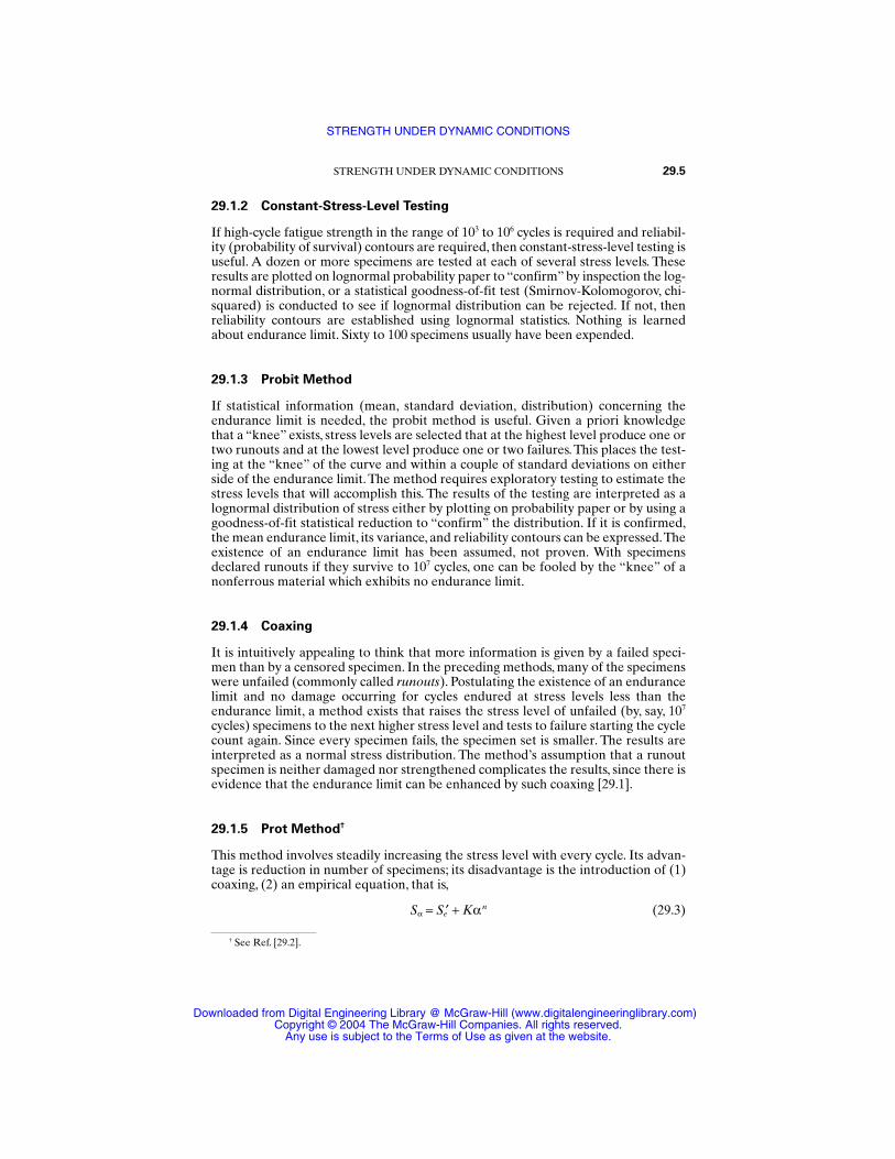
29.1.2 Constant-Stress-Level Testing
If high-cycle fatigue strength in the range of 103 to 106 cycles is required and reliabil-ity (probability of survival) contours are required, then constant-stress-level testing isuseful. A dozen or more specimens are tested at each of several stress levels. Theseresults are plotted on lognormal probability paper to “confirm” by inspection the log-normal distribution, or a statistical goodness-of-fit test (Smirnov-Kolomogorov, chi-squared) is conducted to see if lognormal distribution can be rejected. If not, thenreliability contours are established using lognormal statistics. Nothing is learnedabout endurance limit. Sixty to 100 specimens usually have been expended.
29.1.3 Probit Method
If statistical information (mean, standard deviation, distribution) concerning theendurance limit is needed, the probit method is useful. Given a priori knowledgethat a “knee” exists, stress levels are selected that at the highest level produce one ortwo runouts and at the lowest level produce one or two failures. This places the test-ing at the “knee” of the curve and within a couple of standard deviations on eitherside of the endurance limit. The method requires exploratory testing to estimate thestress levels that will accomplish this. The results of the testing are interpreted as alognormal distribution of stress either by plotting on probability paper or by using agoodness-of-fit statistical reduction to “confirm” the distribution. If it is confirmed,the mean endurance limit, its variance, and reliability contours can be expressed.Theexistence of an endurance limit has been assumed, not proven. With specimensdeclared runouts if they survive to 107 cycles, one can be fooled by the “knee” of anonferrous material which exhibits no endurance limit.
29.1.4 Coaxing
It is intuitively appealing to think that more information is given by a failed speci-men than by a censored specimen. In the preceding methods, many of the specimenswere unfailed (commonly called runouts). Postulating the existence of an endurancelimit and no damage occurring for cycles endured at stress levels less than theendurance limit, a method exists that raises the stress level of unfailed (by, say, 107
cycles) specimens to the next higher stress level and tests to failure starting the cyclecount again. Since every specimen fails, the specimen set is smaller. The results areinterpreted as a normal stress distribution. The method’s assumption that a runoutspecimen is neither damaged nor strengthened complicates the results, since there isevidence that the endurance limit can be enhanced by such coaxing [29.1].
29.1.5 Prot Method†
This method involves steadily increasing the stress level with every cycle. Its advan-tage is reduction in number of specimens; its disadvantage is the introduction of (1)coaxing, (2) an empirical equation, that is,
Sα = Se′ + Kαn (29.3)
STRENGTH UNDER DYNAMIC CONDITIONS 29.5
† See Ref. [29.2].
STRENGTH UNDER DYNAMIC CONDITIONS
Downloaded from Digital Engineering Library @ McGraw-Hill (www.digitalengineeringlibrary.com)Copyright © 2004 The McGraw-Hill Companies. All rights reserved.
Any use is subject to the Terms of Use as given at the website.
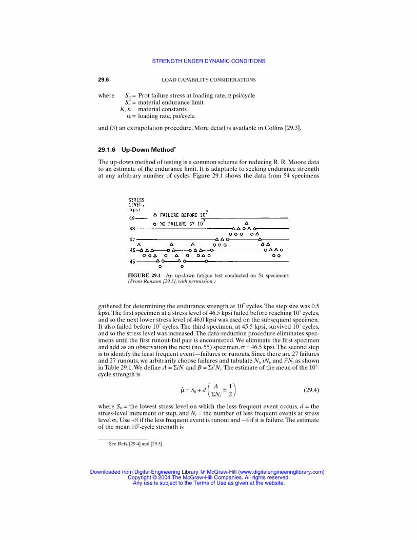
where Sα = Prot failure stress at loading rate, α psi/cycleSe′ = material endurance limit
K, n = material constantsα = loading rate, psi/cycle
and (3) an extrapolation procedure. More detail is available in Collins [29.3].
29.1.6 Up-Down Method†
The up-down method of testing is a common scheme for reducing R. R. Moore datato an estimate of the endurance limit. It is adaptable to seeking endurance strengthat any arbitrary number of cycles. Figure 29.1 shows the data from 54 specimens
29.6 LOAD CAPABILITY CONSIDERATIONS
† See Refs. [29.4] and [29.5].
FIGURE 29.1 An up-down fatigue test conducted on 54 specimens.(From Ransom [29.5], with permission.)
gathered for determining the endurance strength at 107 cycles. The step size was 0.5kpsi.The first specimen at a stress level of 46.5 kpsi failed before reaching 107 cycles,and so the next lower stress level of 46.0 kpsi was used on the subsequent specimen.It also failed before 107 cycles. The third specimen, at 45.5 kpsi, survived 107 cycles,and so the stress level was increased.The data-reduction procedure eliminates spec-imens until the first runout-fail pair is encountered. We eliminate the first specimenand add as an observation the next (no. 55) specimen, σ = 46.5 kpsi. The second stepis to identify the least frequent event—failures or runouts. Since there are 27 failuresand 27 runouts, we arbitrarily choose failures and tabulate Ni, iNi, and i2Ni as shownin Table 29.1. We define A = ΣiNi and B = Σi2Ni. The estimate of the mean of the 107-cycle strength is
µ = S0 + d ± (29.4)
where S0 = the lowest stress level on which the less frequent event occurs, d = thestress-level increment or step, and Ni = the number of less frequent events at stresslevel σi. Use +1⁄2 if the less frequent event is runout and −1⁄2 if it is failure.The estimateof the mean 107-cycle strength is
12
AΣNi
STRENGTH UNDER DYNAMIC CONDITIONS
Downloaded from Digital Engineering Library @ McGraw-Hill (www.digitalengineeringlibrary.com)Copyright © 2004 The McGraw-Hill Companies. All rights reserved.
Any use is subject to the Terms of Use as given at the website.
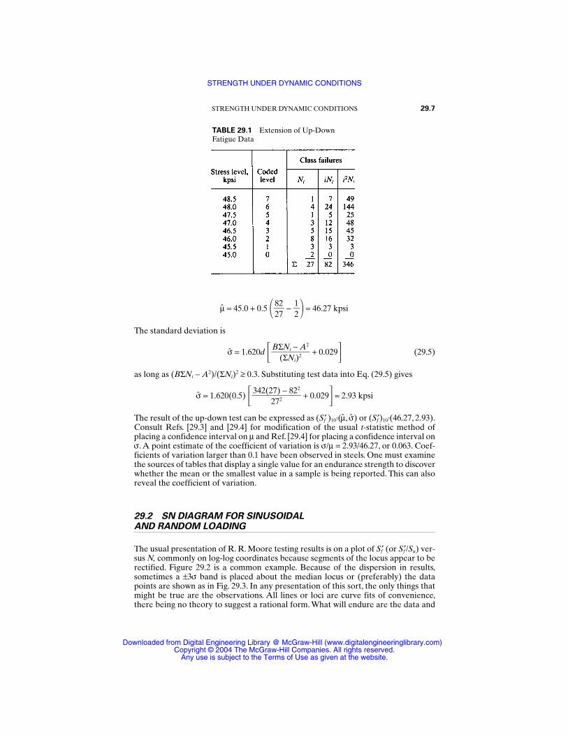
µ = 45.0 + 0.5 − = 46.27 kpsi
The standard deviation is
å = 1.620d + 0.029 (29.5)
as long as (BΣNi − A2)/(ΣNi)2 ≥ 0.3. Substituting test data into Eq. (29.5) gives
å = 1.620(0.5) + 0.029 = 2.93 kpsi
The result of the up-down test can be expressed as (Sf′ )107(µ,å) or (Sf′)107(46.27, 2.93).Consult Refs. [29.3] and [29.4] for modification of the usual t-statistic method ofplacing a confidence interval on µ and Ref. [29.4] for placing a confidence interval onç. A point estimate of the coefficient of variation is ç/µ = 2.93/46.27, or 0.063. Coef-ficients of variation larger than 0.1 have been observed in steels. One must examinethe sources of tables that display a single value for an endurance strength to discoverwhether the mean or the smallest value in a sample is being reported. This can alsoreveal the coefficient of variation.
29.2 SN DIAGRAM FOR SINUSOIDAL AND RANDOM LOADING
The usual presentation of R. R. Moore testing results is on a plot of Sf′ (or Sf′/Su) ver-sus N, commonly on log-log coordinates because segments of the locus appear to berectified. Figure 29.2 is a common example. Because of the dispersion in results,sometimes a ±3ç band is placed about the median locus or (preferably) the datapoints are shown as in Fig. 29.3. In any presentation of this sort, the only things thatmight be true are the observations. All lines or loci are curve fits of convenience,there being no theory to suggest a rational form. What will endure are the data and
342(27) − 822
272
BΣNi − A2
(ΣNi)2
12
8227
STRENGTH UNDER DYNAMIC CONDITIONS 29.7
TABLE 29.1 Extension of Up-DownFatigue Data
STRENGTH UNDER DYNAMIC CONDITIONS
Downloaded from Digital Engineering Library @ McGraw-Hill (www.digitalengineeringlibrary.com)Copyright © 2004 The McGraw-Hill Companies. All rights reserved.
Any use is subject to the Terms of Use as given at the website.
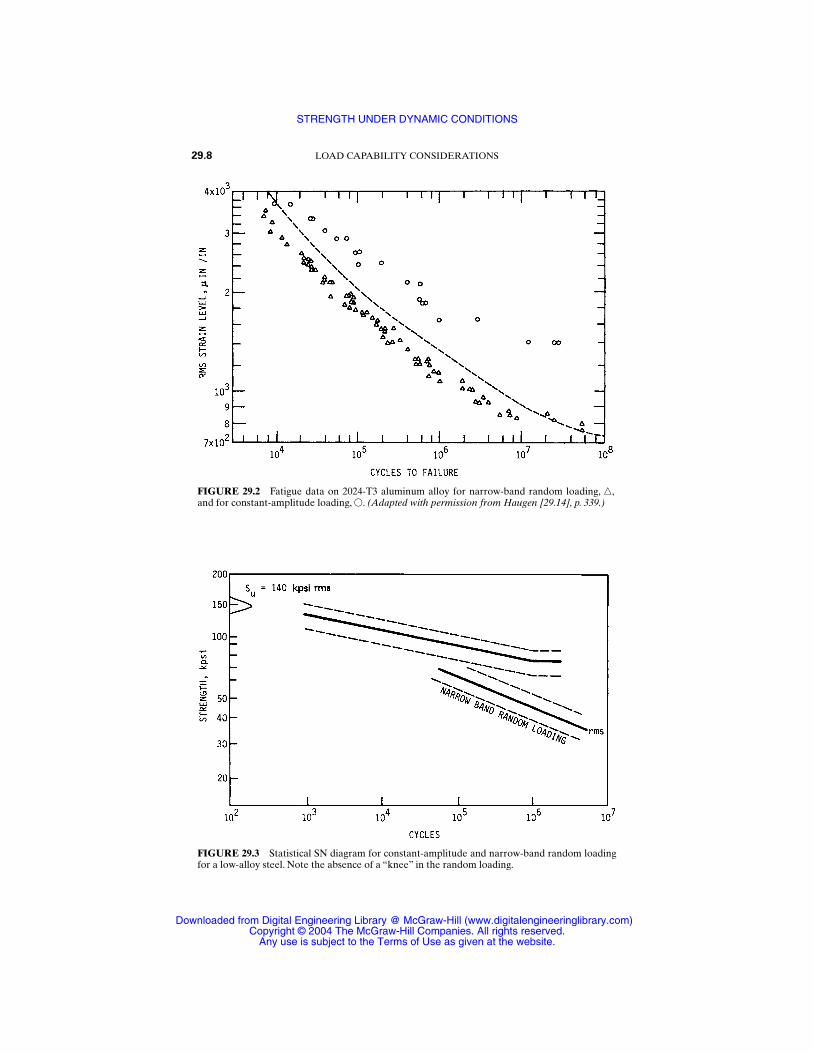
29.8 LOAD CAPABILITY CONSIDERATIONS
FIGURE 29.2 Fatigue data on 2024-T3 aluminum alloy for narrow-band random loading, ,and for constant-amplitude loading, . (Adapted with permission from Haugen [29.14], p. 339.)
FIGURE 29.3 Statistical SN diagram for constant-amplitude and narrow-band random loadingfor a low-alloy steel. Note the absence of a “knee” in the random loading.
STRENGTH UNDER DYNAMIC CONDITIONS
Downloaded from Digital Engineering Library @ McGraw-Hill (www.digitalengineeringlibrary.com)Copyright © 2004 The McGraw-Hill Companies. All rights reserved.
Any use is subject to the Terms of Use as given at the website.
not the loci. Unfortunately, too much reported work is presented without data;hence early effort is largely lost as we learn more.
The R. R. Moore test is a sinusoidal completely reversed flexural loading, which istypical of much rotating machinery, but not of other forms of fatigue. Narrow-bandrandom loading (zero mean) exhibits a lower strength than constant-amplitude sine-wave loading. Figure 29.3 is an example of a distributional presentation, and Fig. 29.2shows the difference between sinusoidal and random-loading strength.
29.3 FATIGUE-STRENGTH MODIFICATION FACTORS
The results of endurance testing are often made available to the designer in a con-cise form by metals suppliers and company materials sections. Plotting coordinatesare chosen so that it is just as easy to enter the plot with maximum-stress, minimum-stress information as steady and alternating stresses. The failure contours areindexed from about 103 cycles up to about 109 cycles. Figures 29.4, 29.5, and 29.6 are
STRENGTH UNDER DYNAMIC CONDITIONS 29.9
FIGURE 29.4 Fatigue-strength diagram for 2024-T3, 2024-T4, and 2014-T6 aluminum alloys,axial loading. Average of test data for polished specimens (unclad) from rolled and drawnsheet and bar. Static properties for 2024: Su = 72 kpsi, Sy = 52 kpsi; for 2014: Su = 72 kpsi, Sy = 63kpsi. (Grumman Aerospace Corp.)
examples. The usual testing basis is bending fatigue, zero mean, constant amplitude.Figure 29.6 represents axial fatigue. The problem for the designer is how to adjustthis information to account for all the discrepancies between the R. R. Moore spec-imen and the contemplated machine part.The Marin approach [29.6] is to introducemultiplicative modification factors to adjust the endurance limit, in the determinis-tic form
Se = kakbkckdkeSe′ (29.6)
STRENGTH UNDER DYNAMIC CONDITIONS
Downloaded from Digital Engineering Library @ McGraw-Hill (www.digitalengineeringlibrary.com)Copyright © 2004 The McGraw-Hill Companies. All rights reserved.
Any use is subject to the Terms of Use as given at the website.
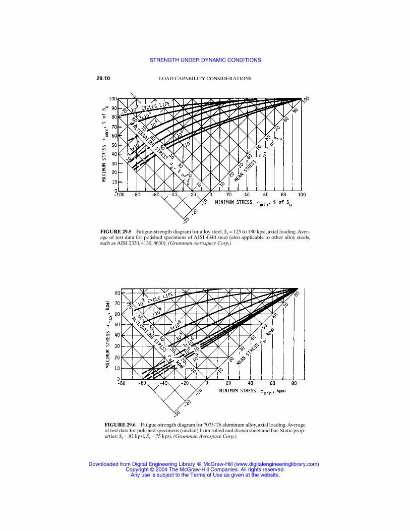
29.10 LOAD CAPABILITY CONSIDERATIONS
FIGURE 29.5 Fatigue-strength diagram for alloy steel, Su = 125 to 180 kpsi, axial loading. Aver-age of test data for polished specimens of AISI 4340 steel (also applicable to other alloy steels,such as AISI 2330, 4130, 8630). (Grumman Aerospace Corp.)
FIGURE 29.6 Fatigue-strength diagram for 7075-T6 aluminum alloy, axial loading.Averageof test data for polished specimens (unclad) from rolled and drawn sheet and bar. Static prop-erties: Su = 82 kpsi, Sy = 75 kpsi. (Grumman Aerospace Corp.)
STRENGTH UNDER DYNAMIC CONDITIONS
Downloaded from Digital Engineering Library @ McGraw-Hill (www.digitalengineeringlibrary.com)Copyright © 2004 The McGraw-Hill Companies. All rights reserved.
Any use is subject to the Terms of Use as given at the website.
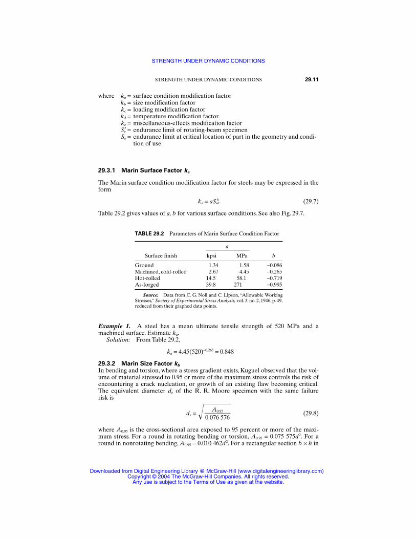
where ka = surface condition modification factorkb = size modification factorkc = loading modification factorkd = temperature modification factorke = miscellaneous-effects modification factorSe′ = endurance limit of rotating-beam specimenSe = endurance limit at critical location of part in the geometry and condi-
tion of use
29.3.1 Marin Surface Factor ka
The Marin surface condition modification factor for steels may be expressed in theform
ka = aSutb (29.7)
Table 29.2 gives values of a, b for various surface conditions. See also Fig. 29.7.
STRENGTH UNDER DYNAMIC CONDITIONS 29.11
Example 1. A steel has a mean ultimate tensile strength of 520 MPa and amachined surface. Estimate ka.
Solution: From Table 29.2,
ka = 4.45(520)−0.265 = 0.848
29.3.2 Marin Size Factor kb
In bending and torsion, where a stress gradient exists, Kuguel observed that the vol-ume of material stressed to 0.95 or more of the maximum stress controls the risk ofencountering a crack nucleation, or growth of an existing flaw becoming critical.The equivalent diameter de of the R. R. Moore specimen with the same failure risk is
de = (29.8)
where A0.95 is the cross-sectional area exposed to 95 percent or more of the maxi-mum stress. For a round in rotating bending or torsion, A0.95 = 0.075 575d2. For around in nonrotating bending, A0.95 = 0.010 462d2. For a rectangular section b × h in
A0.950.076 576
TABLE 29.2 Parameters of Marin Surface Condition Factor
a
Surface finish kpsi MPa b
Ground 1.34 1.58 −0.086Machined, cold-rolled 2.67 4.45 −0.265Hot-rolled 14.5 58.1 −0.719As-forged 39.8 271 −0.995
Source: Data from C. G. Noll and C. Lipson, “Allowable WorkingStresses,” Society of Experimental Stress Analysis, vol. 3, no. 2, 1946, p. 49,reduced from their graphed data points.
STRENGTH UNDER DYNAMIC CONDITIONS
Downloaded from Digital Engineering Library @ McGraw-Hill (www.digitalengineeringlibrary.com)Copyright © 2004 The McGraw-Hill Companies. All rights reserved.
Any use is subject to the Terms of Use as given at the website.
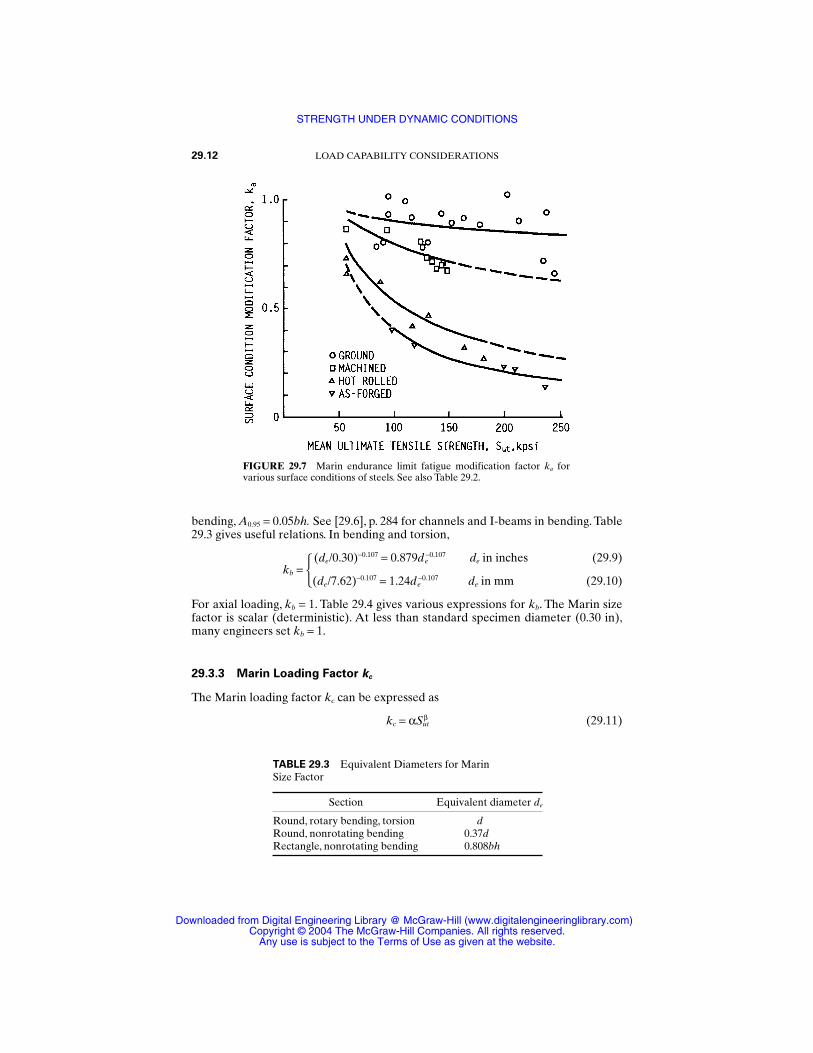
bending, A0.95 = 0.05bh. See [29.6], p. 284 for channels and I-beams in bending. Table29.3 gives useful relations. In bending and torsion,
kb = (de/0.30)−0.107 = 0.879de−0.107 de in inches (29.9)
(de/7.62)−0.107 = 1.24de−0.107 de in mm (29.10)
For axial loading, kb = 1. Table 29.4 gives various expressions for kb. The Marin sizefactor is scalar (deterministic). At less than standard specimen diameter (0.30 in),many engineers set kb = 1.
29.3.3 Marin Loading Factor kc
The Marin loading factor kc can be expressed as
kc = αSutβ (29.11)
29.12 LOAD CAPABILITY CONSIDERATIONS
FIGURE 29.7 Marin endurance limit fatigue modification factor ka forvarious surface conditions of steels. See also Table 29.2.
TABLE 29.3 Equivalent Diameters for Marin Size Factor
Section Equivalent diameter de
Round, rotary bending, torsion dRound, nonrotating bending 0.37dRectangle, nonrotating bending 0.808bh
STRENGTH UNDER DYNAMIC CONDITIONS
Downloaded from Digital Engineering Library @ McGraw-Hill (www.digitalengineeringlibrary.com)Copyright © 2004 The McGraw-Hill Companies. All rights reserved.
Any use is subject to the Terms of Use as given at the website.
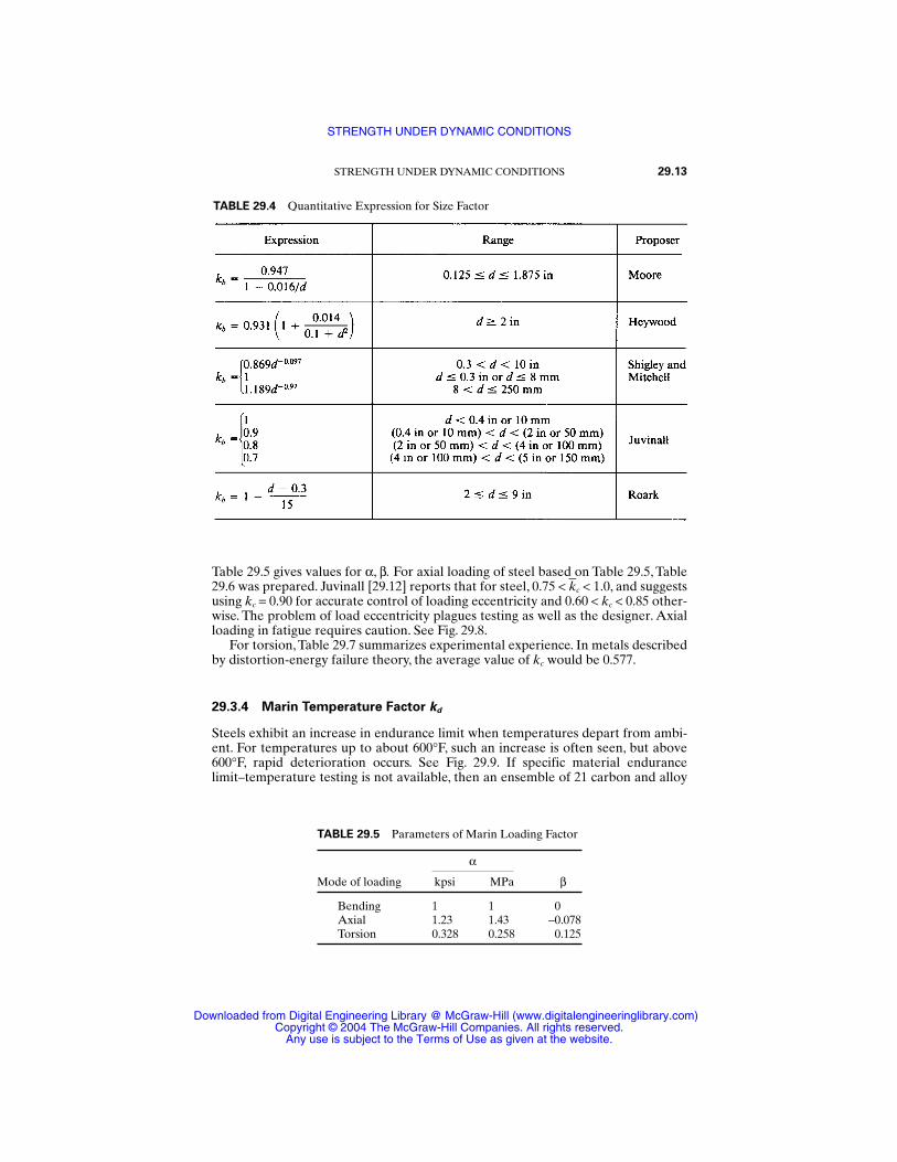
Table 29.5 gives values for α, β. For axial loading of steel based on Table 29.5, Table29.6 was prepared. Juvinall [29.12] reports that for steel, 0.75 < kc < 1.0, and suggestsusing kc = 0.90 for accurate control of loading eccentricity and 0.60 < kc < 0.85 other-wise. The problem of load eccentricity plagues testing as well as the designer. Axialloading in fatigue requires caution. See Fig. 29.8.
For torsion, Table 29.7 summarizes experimental experience. In metals describedby distortion-energy failure theory, the average value of kc would be 0.577.
29.3.4 Marin Temperature Factor kd
Steels exhibit an increase in endurance limit when temperatures depart from ambi-ent. For temperatures up to about 600°F, such an increase is often seen, but above600°F, rapid deterioration occurs. See Fig. 29.9. If specific material endurancelimit–temperature testing is not available, then an ensemble of 21 carbon and alloy
STRENGTH UNDER DYNAMIC CONDITIONS 29.13
TABLE 29.4 Quantitative Expression for Size Factor
TABLE 29.5 Parameters of Marin Loading Factor
α
Mode of loading kpsi MPa β
Bending 1 1 0Axial 1.23 1.43 −0.078Torsion 0.328 0.258 0.125
STRENGTH UNDER DYNAMIC CONDITIONS
Downloaded from Digital Engineering Library @ McGraw-Hill (www.digitalengineeringlibrary.com)Copyright © 2004 The McGraw-Hill Companies. All rights reserved.
Any use is subject to the Terms of Use as given at the website.
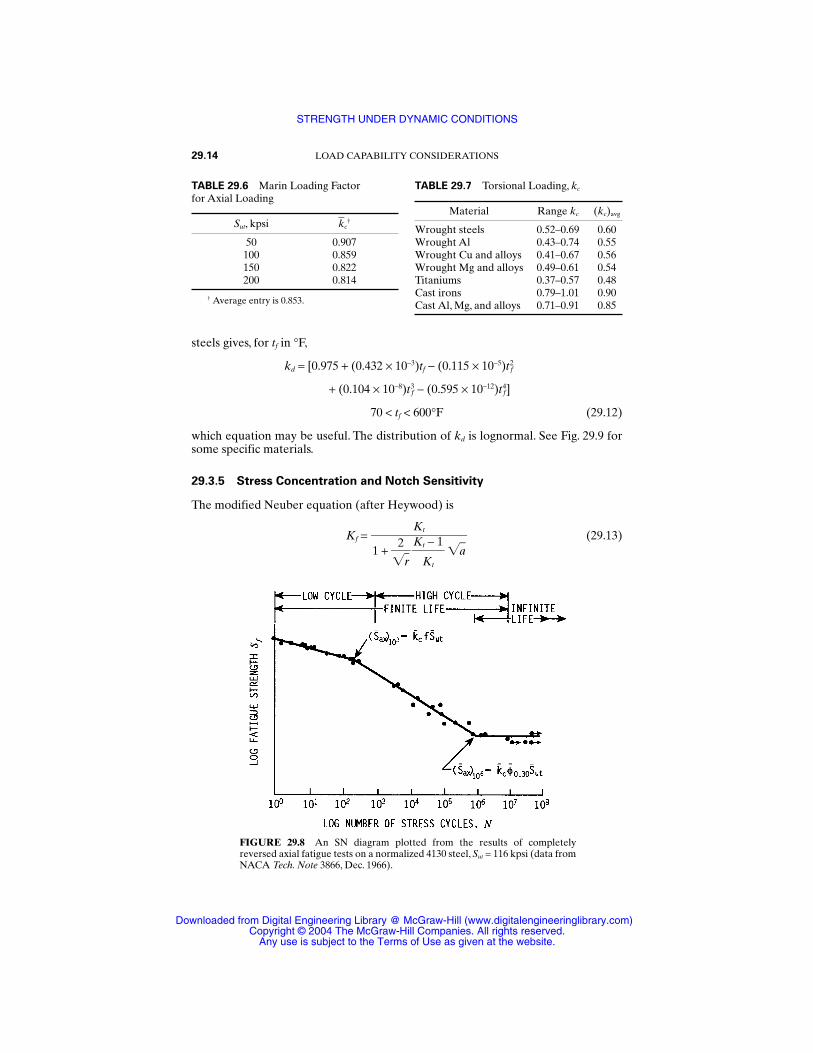
29.14 LOAD CAPABILITY CONSIDERATIONS
TABLE 29.6 Marin Loading Factor for Axial Loading
Sut, kpsi kc†
50 0.907100 0.859150 0.822200 0.814
† Average entry is 0.853.
TABLE 29.7 Torsional Loading, kc
Material Range kc (kc)avg
Wrought steels 0.52–0.69 0.60Wrought Al 0.43–0.74 0.55Wrought Cu and alloys 0.41–0.67 0.56Wrought Mg and alloys 0.49–0.61 0.54Titaniums 0.37–0.57 0.48Cast irons 0.79–1.01 0.90Cast Al, Mg, and alloys 0.71–0.91 0.85
FIGURE 29.8 An SN diagram plotted from the results of completelyreversed axial fatigue tests on a normalized 4130 steel, Sut = 116 kpsi (data fromNACA Tech. Note 3866, Dec. 1966).
steels gives, for tf in °F,
kd = [0.975 + (0.432 × 10⁻³)tf − (0.115 × 10⁻⁵)t f2
+ (0.104 × 10⁻⁸)t f3 − (0.595 × 10⁻¹²)t f
4]
70 < tf < 600°F (29.12)
which equation may be useful. The distribution of kd is lognormal. See Fig. 29.9 forsome specific materials.
29.3.5 Stress Concentration and Notch Sensitivity
The modified Neuber equation (after Heywood) is
Kf = (29.13)Kt
1 + 2
r
K
K
t −
t
1 a
STRENGTH UNDER DYNAMIC CONDITIONS
Downloaded from Digital Engineering Library @ McGraw-Hill (www.digitalengineeringlibrary.com)Copyright © 2004 The McGraw-Hill Companies. All rights reserved.
Any use is subject to the Terms of Use as given at the website.
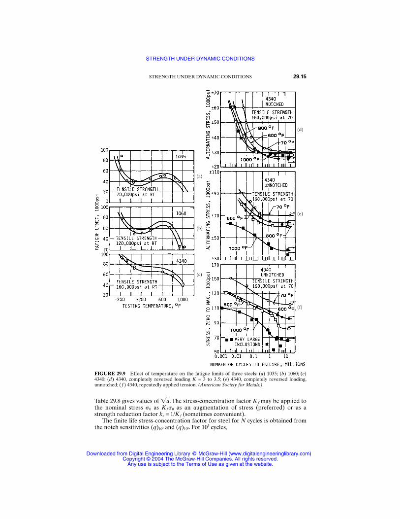
Table 29.8 gives values of a. The stress-concentration factor Kf may be applied tothe nominal stress 0 as Kf0 as an augmentation of stress (preferred) or as astrength reduction factor ke = 1/Kf (sometimes convenient).
The finite life stress-concentration factor for steel for N cycles is obtained fromthe notch sensitivities (q)103 and (q)106. For 103 cycles,
STRENGTH UNDER DYNAMIC CONDITIONS 29.15
FIGURE 29.9 Effect of temperature on the fatigue limits of three steels: (a) 1035; (b) 1060; (c)4340; (d) 4340, completely reversed loading K = 3 to 3.5; (e) 4340, completely reversed loading,unnotched; (f ) 4340, repeatedly applied tension. (American Society for Metals.)
(a)
(b)
(c)
(d)
(e)
(f)
STRENGTH UNDER DYNAMIC CONDITIONS
Downloaded from Digital Engineering Library @ McGraw-Hill (www.digitalengineeringlibrary.com)Copyright © 2004 The McGraw-Hill Companies. All rights reserved.
Any use is subject to the Terms of Use as given at the website.
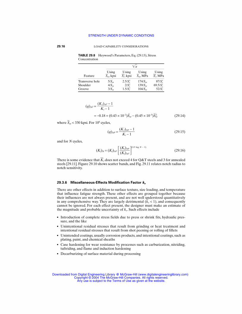
(q)103 =
= −0.18 + (0.43 × 10⁻²)Sut − (0.45 × 10⁻⁵)Sut2 (29.14)
where Sut < 330 kpsi. For 106 cycles,
(q)106 = (29.15)
and for N cycles,
(Kf)N = (Kf)103 (1/3 log N − 1)
(29.16)
There is some evidence that K f does not exceed 4 for Q&T steels and 3 for annealedsteels [29.11]. Figure 29.10 shows scatter bands, and Fig. 29.11 relates notch radius tonotch sensitivity.
29.3.6 Miscellaneous-Effects Modification Factor ke
There are other effects in addition to surface texture, size loading, and temperaturethat influence fatigue strength. These other effects are grouped together becausetheir influences are not always present, and are not well understood quantitativelyin any comprehensive way. They are largely detrimental (ke < 1), and consequentlycannot be ignored. For each effect present, the designer must make an estimate ofthe magnitude and probable uncertainty of ke. Such effects include
Introduction of complete stress fields due to press or shrink fits, hydraulic pres-sure, and the like
Unintentional residual stresses that result from grinding or heat treatment andintentional residual stresses that result from shot peening or rolling of fillets
Unintended coatings, usually corrosion products, and intentional coatings, such asplating, paint, and chemical sheaths
Case hardening for wear resistance by processes such as carburization, nitriding,tuftriding, and flame and induction hardening
Decarburizing of surface material during processing
(Kf)106
(Kf)103
(Kf)106 − 1
Kt − 1
(Kf)103 − 1
Kt − 1
29.16 LOAD CAPABILITY CONSIDERATIONS
TABLE 29.8 Heywood’s Parameters, Eq. (29.13), Stress Concentration
a
Using Using Using Using Feature Sut, kpsi Se′, kpsi Sut, MPa Se′, MPa
Transverse hole 5/Sut 2.5/Se′ 174/Sut 87/Se′Shoulder 4/Sut 2/Se′ 139/Sut 69.5/Se′Groove 3/Sut 1.5/Se′ 104/Sut 52/Se′
STRENGTH UNDER DYNAMIC CONDITIONS
Downloaded from Digital Engineering Library @ McGraw-Hill (www.digitalengineeringlibrary.com)Copyright © 2004 The McGraw-Hill Companies. All rights reserved.
Any use is subject to the Terms of Use as given at the website.
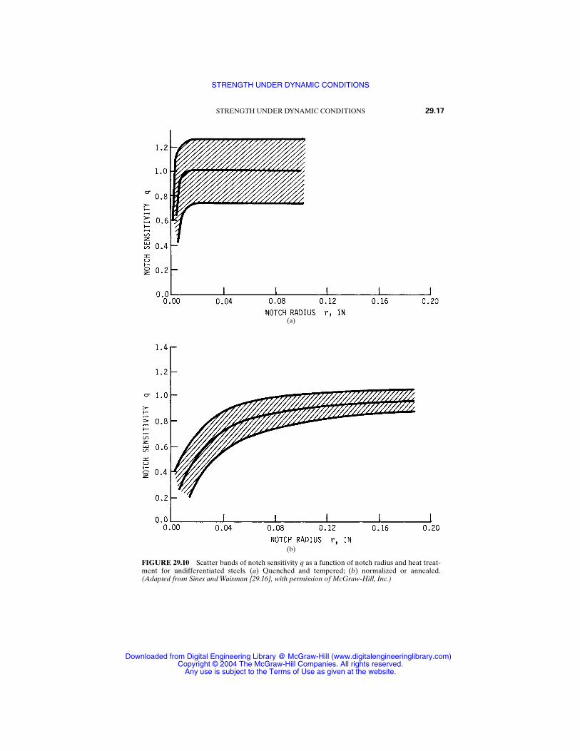
STRENGTH UNDER DYNAMIC CONDITIONS 29.17
FIGURE 29.10 Scatter bands of notch sensitivity q as a function of notch radius and heat treat-ment for undifferentiated steels. (a) Quenched and tempered; (b) normalized or annealed.(Adapted from Sines and Waisman [29.16], with permission of McGraw-Hill, Inc.)
(b)
(a)
STRENGTH UNDER DYNAMIC CONDITIONS
Downloaded from Digital Engineering Library @ McGraw-Hill (www.digitalengineeringlibrary.com)Copyright © 2004 The McGraw-Hill Companies. All rights reserved.
Any use is subject to the Terms of Use as given at the website.
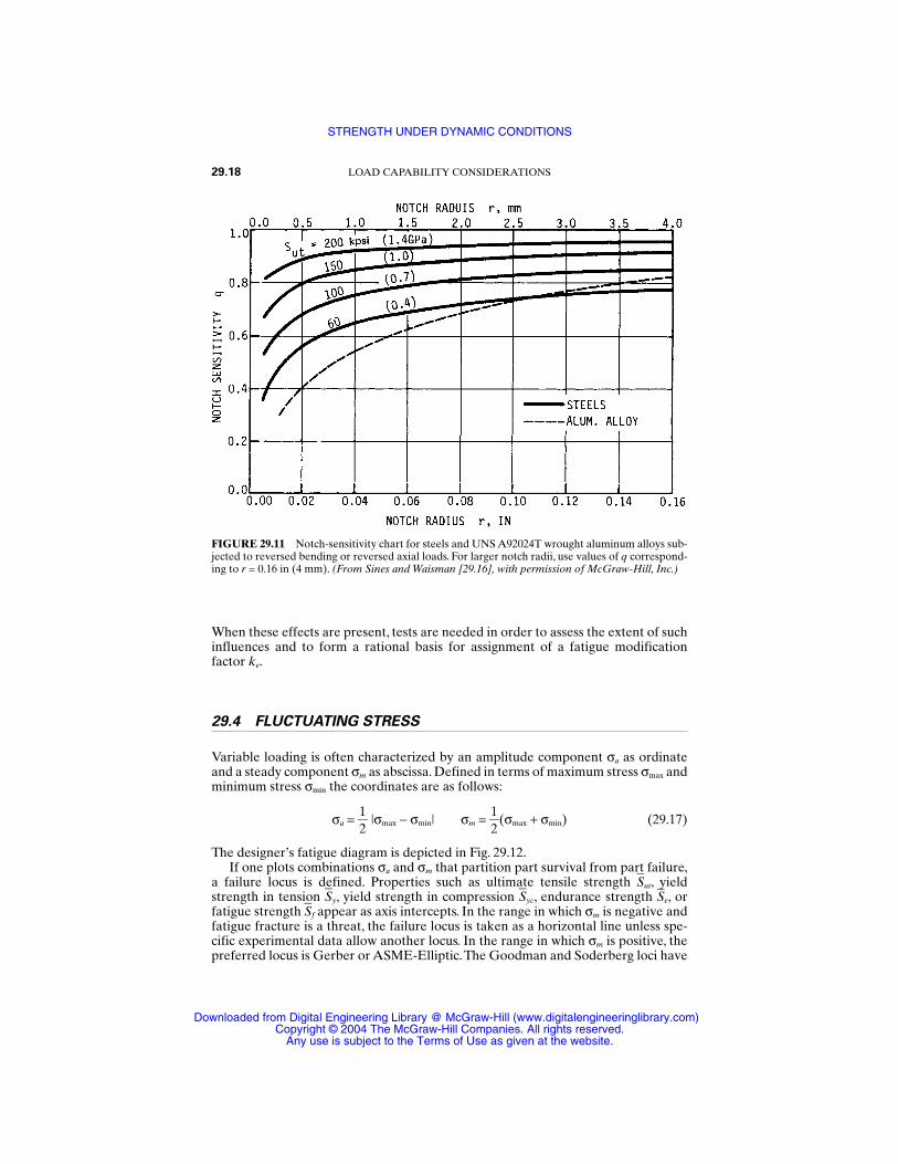
When these effects are present, tests are needed in order to assess the extent of suchinfluences and to form a rational basis for assignment of a fatigue modification factor ke.
29.4 FLUCTUATING STRESS
Variable loading is often characterized by an amplitude component σa as ordinateand a steady component σm as abscissa. Defined in terms of maximum stress σmax andminimum stress σmin the coordinates are as follows:
σa = 12
|σmax − σmin| σm = 12
(σmax + σmin) (29.17)
The designer’s fatigue diagram is depicted in Fig. 29.12.If one plots combinations σa and σm that partition part survival from part failure,
a failure locus is defined. Properties such as ultimate tensile strength Sut, yieldstrength in tension Sy, yield strength in compression Syc, endurance strength Se, orfatigue strength Sf appear as axis intercepts. In the range in which σm is negative andfatigue fracture is a threat, the failure locus is taken as a horizontal line unless spe-cific experimental data allow another locus. In the range in which σm is positive, thepreferred locus is Gerber or ASME-Elliptic.The Goodman and Soderberg loci have
29.18 LOAD CAPABILITY CONSIDERATIONS
FIGURE 29.11 Notch-sensitivity chart for steels and UNS A92024T wrought aluminum alloys sub-jected to reversed bending or reversed axial loads. For larger notch radii, use values of q correspond-ing to r = 0.16 in (4 mm). (From Sines and Waisman [29.16], with permission of McGraw-Hill, Inc.)
STRENGTH UNDER DYNAMIC CONDITIONS
Downloaded from Digital Engineering Library @ McGraw-Hill (www.digitalengineeringlibrary.com)Copyright © 2004 The McGraw-Hill Companies. All rights reserved.
Any use is subject to the Terms of Use as given at the website.
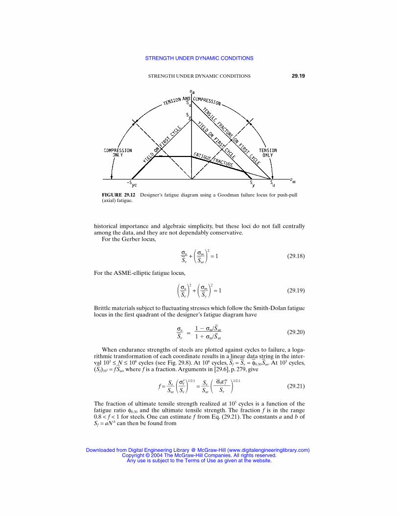
historical importance and algebraic simplicity, but these loci do not fall centrallyamong the data, and they are not dependably conservative.
For the Gerber locus,
+ 2
= 1 (29.18)
For the ASME-elliptic fatigue locus,
σSe
a2
+ σS
m
y
2
= 1 (29.19)
Brittle materials subject to fluctuating stresses which follow the Smith-Dolan fatiguelocus in the first quadrant of the designer’s fatigue diagram have
σSe
a (29.20)
When endurance strengths of steels are plotted against cycles to failure, a loga-rithmic transformation of each coordinate results in a linear data string in the inter-val 103 ≤ N ≤ 106 cycles (see Fig. 29.8). At 106 cycles, Sf = Se = φ0.30Sut. At 103 cycles,(Sf)103 = fSut, where f is a fraction. Arguments in [29.6], p. 279, give
f = SS
u
e
t
σSe
f′
1/2.1
= SS
u
e
t
1/2.1
(29.21)
The fraction of ultimate tensile strength realized at 103 cycles is a function of thefatigue ratio φ0.30 and the ultimate tensile strength. The fraction f is in the range 0.8 < f < 1 for steels. One can estimate f from Eq. (29.21). The constants a and b ofSf = aN b can then be found from
σ0ε fm
Se
1 σm/S–
ut1 σm/S
–ut
σmSut
σaSe
STRENGTH UNDER DYNAMIC CONDITIONS 29.19
FIGURE 29.12 Designer’s fatigue diagram using a Goodman failure locus for push-pull(axial) fatigue.
STRENGTH UNDER DYNAMIC CONDITIONS
Downloaded from Digital Engineering Library @ McGraw-Hill (www.digitalengineeringlibrary.com)Copyright © 2004 The McGraw-Hill Companies. All rights reserved.
Any use is subject to the Terms of Use as given at the website.
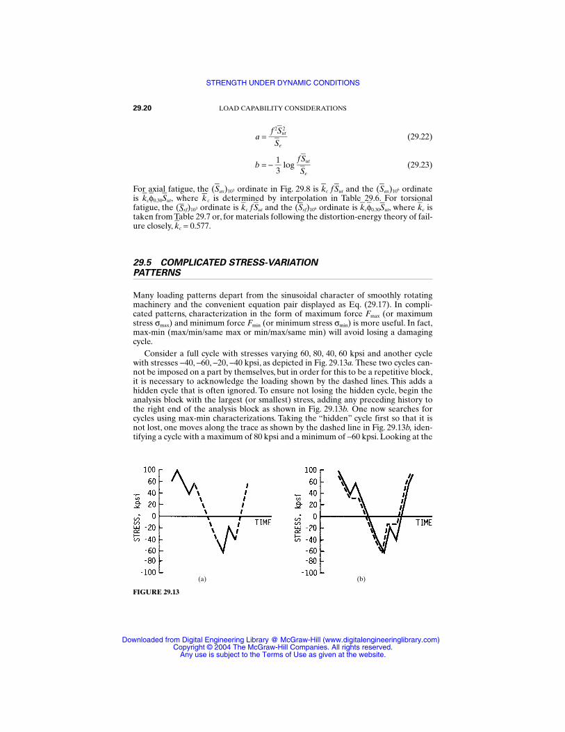
a = (29.22)
b = − 13
log (29.23)
For axial fatigue, the (Sax)103 ordinate in Fig. 29.8 is kc fSut and the (Sax)106 ordinateis kcφ0.30Sut, where kc is determined by interpolation in Table 29.6. For torsionalfatigue, the (Ssf)103 ordinate is kc fSut and the (Ssf)106 ordinate is kcφ0.30Sut, where kc istaken from Table 29.7 or, for materials following the distortion-energy theory of fail-ure closely, kc = 0.577.
29.5 COMPLICATED STRESS-VARIATIONPATTERNS
Many loading patterns depart from the sinusoidal character of smoothly rotatingmachinery and the convenient equation pair displayed as Eq. (29.17). In compli-cated patterns, characterization in the form of maximum force Fmax (or maximumstress σmax) and minimum force Fmin (or minimum stress σmin) is more useful. In fact,max-min (max/min/same max or min/max/same min) will avoid losing a damagingcycle.
Consider a full cycle with stresses varying 60, 80, 40, 60 kpsi and another cyclewith stresses −40, −60, −20, −40 kpsi, as depicted in Fig. 29.13a. These two cycles can-not be imposed on a part by themselves, but in order for this to be a repetitive block,it is necessary to acknowledge the loading shown by the dashed lines. This adds ahidden cycle that is often ignored. To ensure not losing the hidden cycle, begin theanalysis block with the largest (or smallest) stress, adding any preceding history tothe right end of the analysis block as shown in Fig. 29.13b. One now searches forcycles using max-min characterizations. Taking the “hidden” cycle first so that it isnot lost, one moves along the trace as shown by the dashed line in Fig. 29.13b, iden-tifying a cycle with a maximum of 80 kpsi and a minimum of −60 kpsi. Looking at the
fSutSe
f 2Sut2
Se
29.20 LOAD CAPABILITY CONSIDERATIONS
FIGURE 29.13
(a) (b)
STRENGTH UNDER DYNAMIC CONDITIONS
Downloaded from Digital Engineering Library @ McGraw-Hill (www.digitalengineeringlibrary.com)Copyright © 2004 The McGraw-Hill Companies. All rights reserved.
Any use is subject to the Terms of Use as given at the website.
remaining cycles, one notes a cycle with a maximum of 60 and a minimum of 40 kpsi.There is another with a maximum of −20 and a minimum of −40 kpsi. Since failuretheories are expressed in terms of σa and σm components, one uses Eqs. (29.17) andconstructs the table below.
Cycle σmax σmin σa σm
1 80 −60 70 102 60 40 10 503 −20 −40 10 −30
Note that the most damaging cycle, cycle 1, has been identified because care wastaken not to lose it. The method used is a variation of the rainflow counting tech-nique. One is now ready to apply Miner’s rule. Note that if the original cycles weredoubled in the block, there would be five cycles, with the additional two duplicatingcycles 2 and 3 above.
Example 2. The loading of Fig. 29.13a is imposed on a part made of 1045 HR steel.Properties at the critical location are Sut = 92.5 kpsi, Se′ = 46 kpsi, strain-strengtheningcoefficient σ0 = 140 kpsi, true strain at fracture εf = 0.58, and strain-strengtheningexponent m = 0.14. Estimate how many repetitions of the loading block may beapplied if a Gerber fatigue locus is used.
Solution. From Eq. (29.21),
f = SS
u
e
t
1/2.1
= 1/2.1
= 9426.5
1/2.1
= 0.815
From Eq. (29.22), a = = 123.5 kpsi
From Eq. (29.23),
b = − 13
log 0.815
4(692.5) = −0.0715
(Sf)103 = fSut = 0.815(92.5) = 75.39 kpsi
For cycle 1, which has σa = 70 kpsi and σm = 10 kpsi, using Eq. (29.18),
Sf = = = 70.83 kpsi
Since required endurance strength 70.83 kpsi is less than (Sf)103, the number of cyclesexceeds 103.
N1 = 1/b
= 7102.38.35
−1/0.0715
= 2383 cycles
For cycle 2, Sf = 14.1 kpsi and N2 = 1.5(1013) ∞. For cycle 3, Sf = σa = 10 kpsi and N3 = 1.8(1015) ∞. Extend the previous table:
Sfa
701 − (10/92.5)2
σa1 − (σm/Sut)2
0.815292.52
46
140(0.58)0.14
46
σ0εfm
Se
SeSut
σf′Se
STRENGTH UNDER DYNAMIC CONDITIONS 29.21
STRENGTH UNDER DYNAMIC CONDITIONS
Downloaded from Digital Engineering Library @ McGraw-Hill (www.digitalengineeringlibrary.com)Copyright © 2004 The McGraw-Hill Companies. All rights reserved.
Any use is subject to the Terms of Use as given at the website.
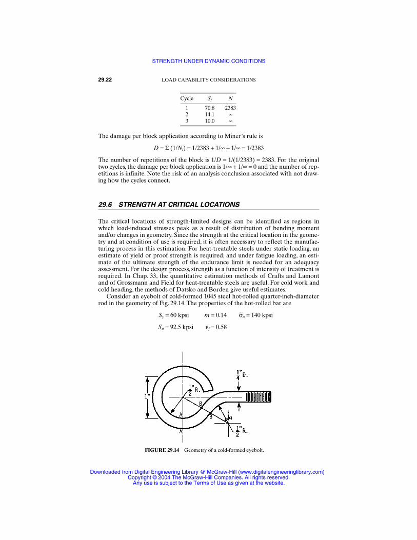
Cycle Sf N
1 70.8 23832 14.1 ∞3 10.0 ∞
The damage per block application according to Miner’s rule is
D = Σ (1/Ni) = 1/2383 + 1/∞ + 1/∞ = 1/2383
The number of repetitions of the block is 1/D = 1/(1/2383) = 2383. For the originaltwo cycles, the damage per block application is 1/∞ + 1/∞ = 0 and the number of rep-etitions is infinite. Note the risk of an analysis conclusion associated with not draw-ing how the cycles connect.
29.6 STRENGTH AT CRITICAL LOCATIONS
The critical locations of strength-limited designs can be identified as regions inwhich load-induced stresses peak as a result of distribution of bending momentand/or changes in geometry. Since the strength at the critical location in the geome-try and at condition of use is required, it is often necessary to reflect the manufac-turing process in this estimation. For heat-treatable steels under static loading, anestimate of yield or proof strength is required, and under fatigue loading, an esti-mate of the ultimate strength of the endurance limit is needed for an adequacyassessment. For the design process, strength as a function of intensity of treatment isrequired. In Chap. 33, the quantitative estimation methods of Crafts and Lamontand of Grossmann and Field for heat-treatable steels are useful. For cold work andcold heading, the methods of Datsko and Borden give useful estimates.
Consider an eyebolt of cold-formed 1045 steel hot-rolled quarter-inch-diameterrod in the geometry of Fig. 29.14. The properties of the hot-rolled bar are
Sy = 60 kpsi m = 0.14 σo = 140 kpsi
Su = 92.5 kpsi εf = 0.58
29.22 LOAD CAPABILITY CONSIDERATIONS
FIGURE 29.14 Geometry of a cold-formed eyebolt.
STRENGTH UNDER DYNAMIC CONDITIONS
Downloaded from Digital Engineering Library @ McGraw-Hill (www.digitalengineeringlibrary.com)Copyright © 2004 The McGraw-Hill Companies. All rights reserved.
Any use is subject to the Terms of Use as given at the website.
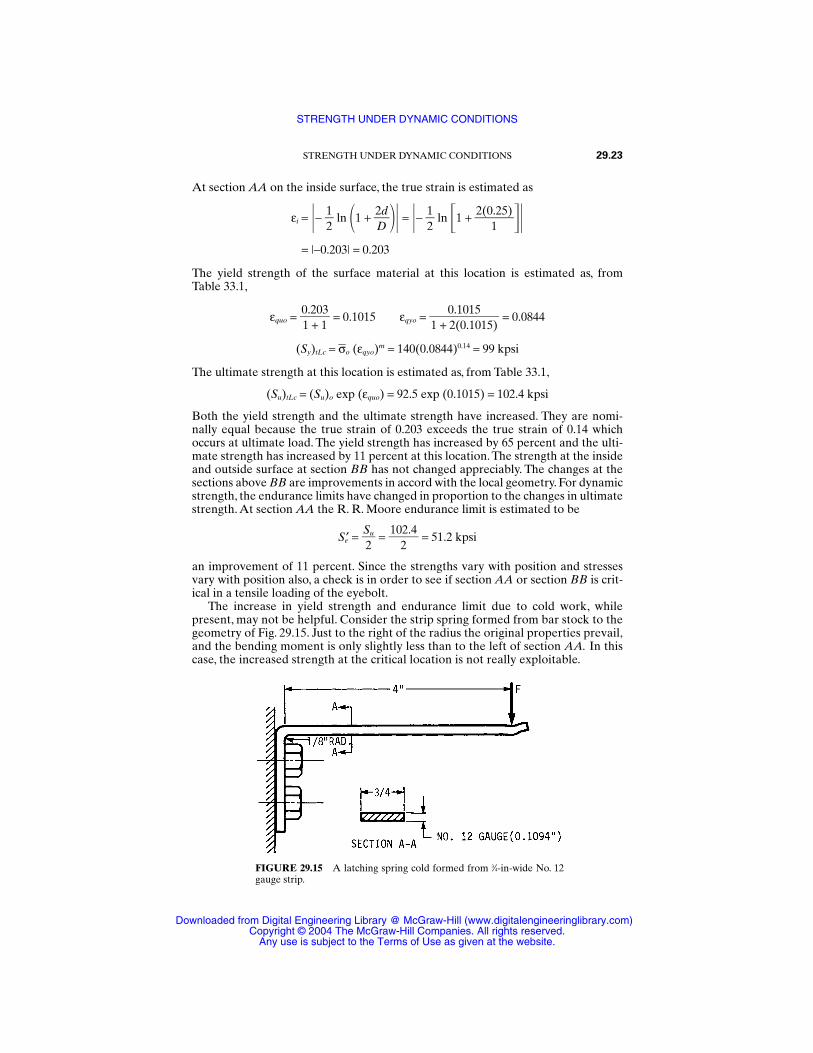
At section AA on the inside surface, the true strain is estimated as
εi = − 12
ln 1 + 2Dd = −
12
ln 1 + 2(0
1.25)
= |−0.203| = 0.203
The yield strength of the surface material at this location is estimated as, from Table 33.1,
εquo = = 0.1015 εqyo = = 0.0844
(Sy)tLc = σo (εqyo)m = 140(0.0844)0.14 = 99 kpsi
The ultimate strength at this location is estimated as, from Table 33.1,
(Su)tLc = (Su)o exp (εquo) = 92.5 exp (0.1015) = 102.4 kpsi
Both the yield strength and the ultimate strength have increased. They are nomi-nally equal because the true strain of 0.203 exceeds the true strain of 0.14 whichoccurs at ultimate load. The yield strength has increased by 65 percent and the ulti-mate strength has increased by 11 percent at this location. The strength at the insideand outside surface at section BB has not changed appreciably. The changes at thesections above BB are improvements in accord with the local geometry. For dynamicstrength, the endurance limits have changed in proportion to the changes in ultimatestrength. At section AA the R. R. Moore endurance limit is estimated to be
Se′ = = = 51.2 kpsi
an improvement of 11 percent. Since the strengths vary with position and stressesvary with position also, a check is in order to see if section AA or section BB is crit-ical in a tensile loading of the eyebolt.
The increase in yield strength and endurance limit due to cold work, whilepresent, may not be helpful. Consider the strip spring formed from bar stock to thegeometry of Fig. 29.15. Just to the right of the radius the original properties prevail,and the bending moment is only slightly less than to the left of section AA. In thiscase, the increased strength at the critical location is not really exploitable.
102.4
2Su2
0.10151 + 2(0.1015)
0.2031 + 1
STRENGTH UNDER DYNAMIC CONDITIONS 29.23
FIGURE 29.15 A latching spring cold formed from 3⁄4-in-wide No. 12gauge strip.
STRENGTH UNDER DYNAMIC CONDITIONS
Downloaded from Digital Engineering Library @ McGraw-Hill (www.digitalengineeringlibrary.com)Copyright © 2004 The McGraw-Hill Companies. All rights reserved.
Any use is subject to the Terms of Use as given at the website.
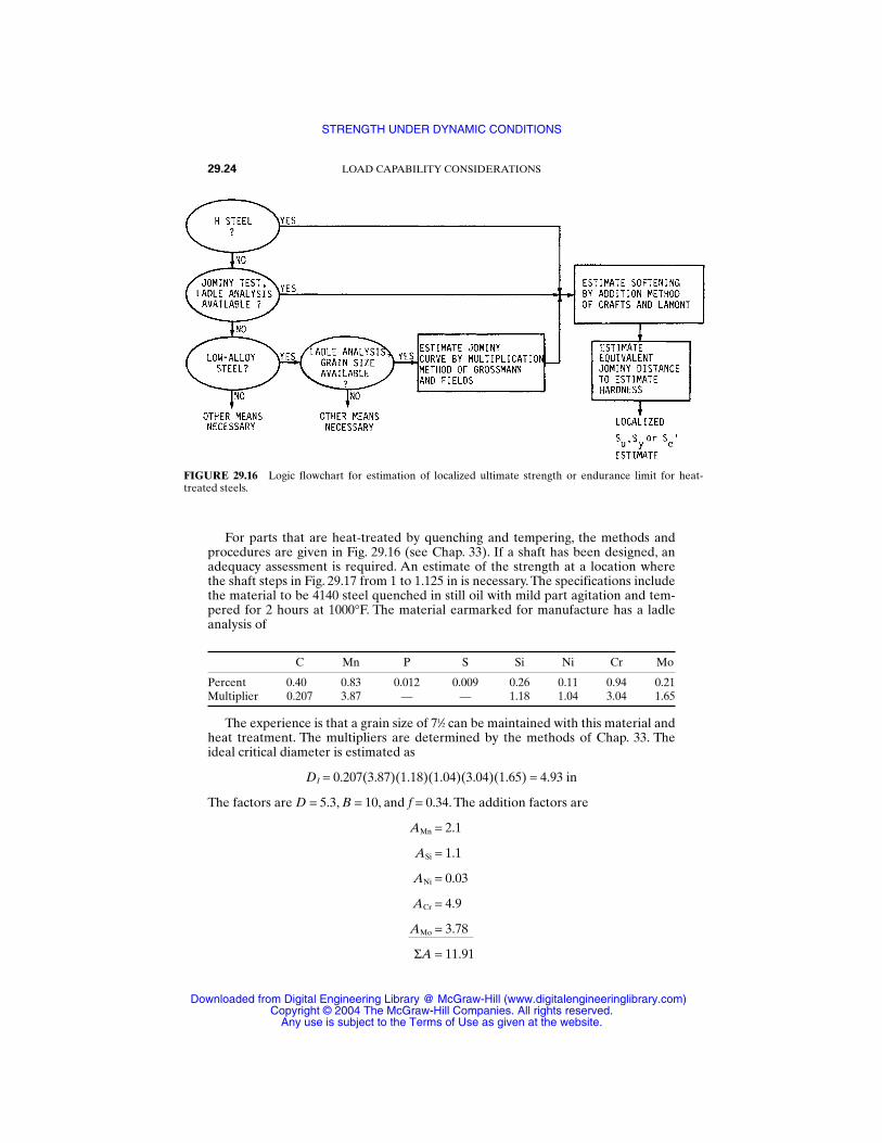
For parts that are heat-treated by quenching and tempering, the methods and procedures are given in Fig. 29.16 (see Chap. 33). If a shaft has been designed, an adequacy assessment is required. An estimate of the strength at a location where the shaft steps in Fig. 29.17 from 1 to 1.125 in is necessary. The specifications includethe material to be 4140 steel quenched in still oil with mild part agitation and tem-pered for 2 hours at 1000°F. The material earmarked for manufacture has a ladleanalysis of
C Mn P S Si Ni Cr Mo
Percent 0.40 0.83 0.012 0.009 0.26 0.11 0.94 0.21Multiplier 0.207 3.87 — — 1.18 1.04 3.04 1.65
The experience is that a grain size of 71⁄2 can be maintained with this material andheat treatment. The multipliers are determined by the methods of Chap. 33. Theideal critical diameter is estimated as
DI = 0.207(3.87)(1.18)(1.04)(3.04)(1.65) = 4.93 in
The factors are D = 5.3, B = 10, and f = 0.34. The addition factors are
AMn = 2.1
ASi = 1.1
ANi = 0.03
ACr = 4.9
AMo = 3.78
ΣA = 11.91
29.24 LOAD CAPABILITY CONSIDERATIONS
FIGURE 29.16 Logic flowchart for estimation of localized ultimate strength or endurance limit for heat-treated steels.
STRENGTH UNDER DYNAMIC CONDITIONS
Downloaded from Digital Engineering Library @ McGraw-Hill (www.digitalengineeringlibrary.com)Copyright © 2004 The McGraw-Hill Companies. All rights reserved.
Any use is subject to the Terms of Use as given at the website.
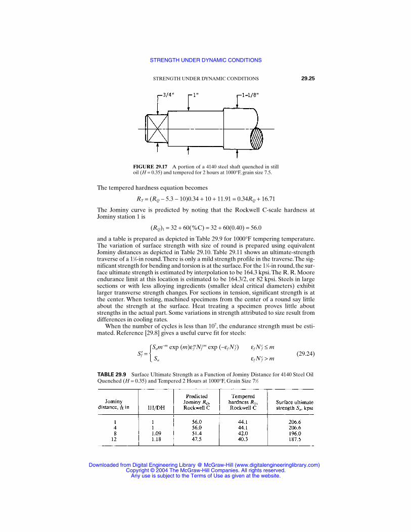
The tempered hardness equation becomes
RT = (RQ − 5.3 − 10)0.34 + 10 + 11.91 = 0.34RQ + 16.71
The Jominy curve is predicted by noting that the Rockwell C-scale hardness atJominy station 1 is
(RQ)1 = 32 + 60(%C) = 32 + 60(0.40) = 56.0
and a table is prepared as depicted in Table 29.9 for 1000°F tempering temperature.The variation of surface strength with size of round is prepared using equivalentJominy distances as depicted in Table 29.10. Table 29.11 shows an ultimate-strengthtraverse of a 11⁄8-in round.There is only a mild strength profile in the traverse.The sig-nificant strength for bending and torsion is at the surface. For the 11⁄8-in round, the sur-face ultimate strength is estimated by interpolation to be 164.3 kpsi.The R. R. Mooreendurance limit at this location is estimated to be 164.3/2, or 82 kpsi. Steels in largesections or with less alloying ingredients (smaller ideal critical diameters) exhibitlarger transverse strength changes. For sections in tension, significant strength is atthe center. When testing, machined specimens from the center of a round say littleabout the strength at the surface. Heat treating a specimen proves little aboutstrengths in the actual part. Some variations in strength attributed to size result fromdifferences in cooling rates.
When the number of cycles is less than 107, the endurance strength must be esti-mated. Reference [29.8] gives a useful curve fit for steels:
Sf′ = Sum−m exp (m)ε fmNf
cm exp (−εf Nfc) εf N f
c ≤ m
Su εf N fc > m
(29.24)
STRENGTH UNDER DYNAMIC CONDITIONS 29.25
FIGURE 29.17 A portion of a 4140 steel shaft quenched in stilloil (H = 0.35) and tempered for 2 hours at 1000°F, grain size 7.5.
TABLE 29.9 Surface Ultimate Strength as a Function of Jominy Distance for 4140 Steel OilQuenched (H = 0.35) and Tempered 2 Hours at 1000°F, Grain Size 71⁄2
STRENGTH UNDER DYNAMIC CONDITIONS
Downloaded from Digital Engineering Library @ McGraw-Hill (www.digitalengineeringlibrary.com)Copyright © 2004 The McGraw-Hill Companies. All rights reserved.
Any use is subject to the Terms of Use as given at the website.
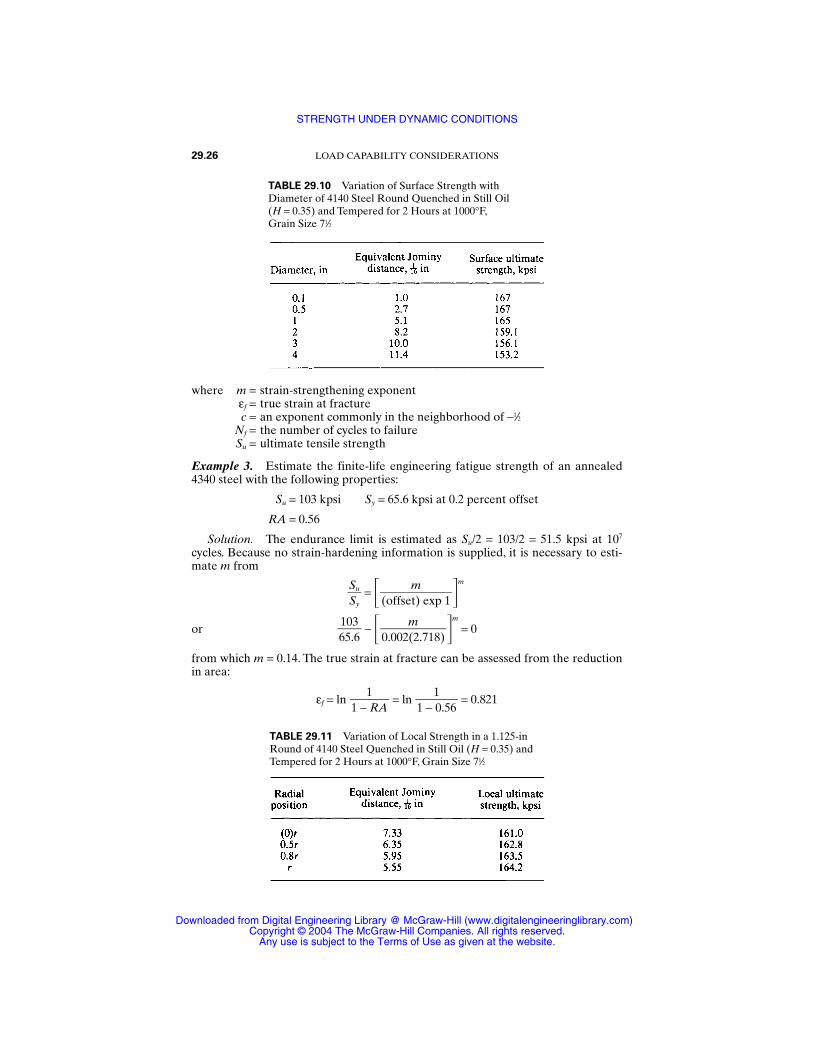
where m = strain-strengthening exponentεf = true strain at fracturec = an exponent commonly in the neighborhood of −1⁄2
Nf = the number of cycles to failureSu = ultimate tensile strength
Example 3. Estimate the finite-life engineering fatigue strength of an annealed4340 steel with the following properties:
Su = 103 kpsi Sy = 65.6 kpsi at 0.2 percent offset
RA = 0.56
Solution. The endurance limit is estimated as Su/2 = 103/2 = 51.5 kpsi at 107
cycles. Because no strain-hardening information is supplied, it is necessary to esti-mate m from
= m
or − m
= 0
from which m = 0.14. The true strain at fracture can be assessed from the reductionin area:
εf = ln = ln = 0.8211
1 − 0.56
11 − RA
m0.002(2.718)
10365.6
m(offset) exp 1
SuSy
29.26 LOAD CAPABILITY CONSIDERATIONS
TABLE 29.10 Variation of Surface Strength with Diameter of 4140 Steel Round Quenched in Still Oil (H = 0.35) and Tempered for 2 Hours at 1000°F,Grain Size 71⁄2
TABLE 29.11 Variation of Local Strength in a 1.125-inRound of 4140 Steel Quenched in Still Oil (H = 0.35) andTempered for 2 Hours at 1000°F, Grain Size 71⁄2
STRENGTH UNDER DYNAMIC CONDITIONS
Downloaded from Digital Engineering Library @ McGraw-Hill (www.digitalengineeringlibrary.com)Copyright © 2004 The McGraw-Hill Companies. All rights reserved.
Any use is subject to the Terms of Use as given at the website.
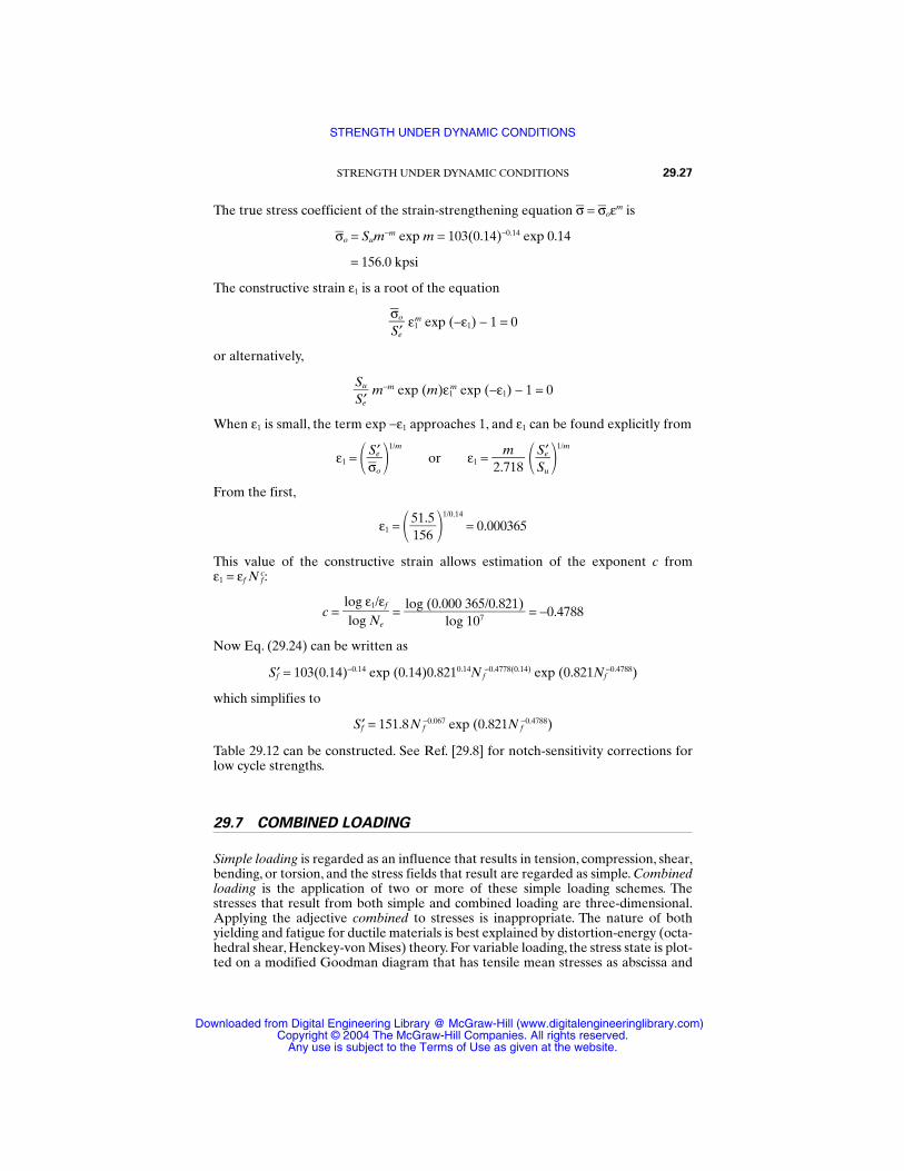
The true stress coefficient of the strain-strengthening equation σ = σoεm is
σo = Sum−m exp m = 103(0.14)−0.14 exp 0.14
= 156.0 kpsi
The constructive strain ε1 is a root of the equation
ε1m exp (−ε1) − 1 = 0
or alternatively,
m−m exp (m)ε1m exp (−ε1) − 1 = 0
When ε1 is small, the term exp −ε1 approaches 1, and ε1 can be found explicitly from
ε1 = 1/m
or ε1 = 1/m
From the first,
ε1 = 1/0.14
= 0.000365
This value of the constructive strain allows estimation of the exponent c fromε1 = εf N f
c:
c = = = −0.4788
Now Eq. (29.24) can be written as
Sf′ = 103(0.14)−0.14 exp (0.14)0.8210.14Nf−0.4778(0.14) exp (0.821Nf
−0.4788)
which simplifies to
Sf′ = 151.8N f−0.067 exp (0.821N f
−0.4788)
Table 29.12 can be constructed. See Ref. [29.8] for notch-sensitivity corrections forlow cycle strengths.
29.7 COMBINED LOADING
Simple loading is regarded as an influence that results in tension, compression, shear,bending, or torsion, and the stress fields that result are regarded as simple. Combinedloading is the application of two or more of these simple loading schemes. Thestresses that result from both simple and combined loading are three-dimensional.Applying the adjective combined to stresses is inappropriate. The nature of bothyielding and fatigue for ductile materials is best explained by distortion-energy (octa-hedral shear, Henckey-von Mises) theory. For variable loading, the stress state is plot-ted on a modified Goodman diagram that has tensile mean stresses as abscissa and
log (0.000 365/0.821)
log 107
log ε1/εflog Ne
51.5156
Se′Su
m2.718
Se′σo
SuSe′
σoSe′
STRENGTH UNDER DYNAMIC CONDITIONS 29.27
STRENGTH UNDER DYNAMIC CONDITIONS
Downloaded from Digital Engineering Library @ McGraw-Hill (www.digitalengineeringlibrary.com)Copyright © 2004 The McGraw-Hill Companies. All rights reserved.
Any use is subject to the Terms of Use as given at the website.
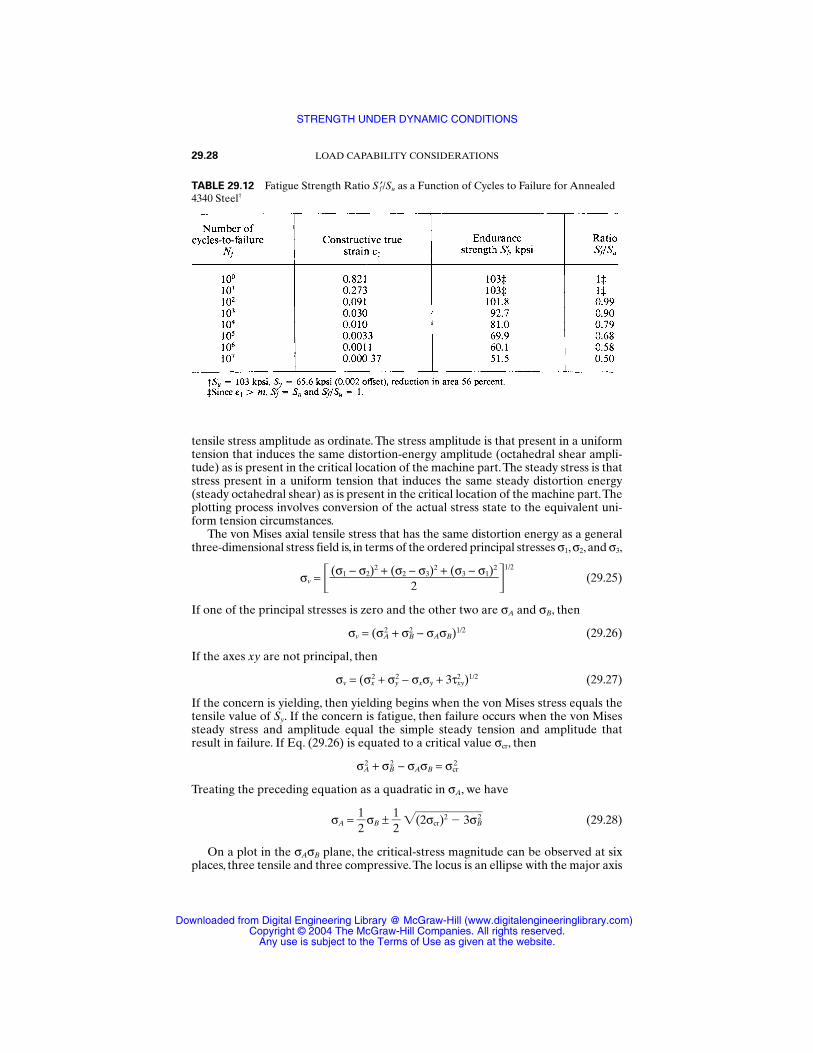
tensile stress amplitude as ordinate. The stress amplitude is that present in a uniformtension that induces the same distortion-energy amplitude (octahedral shear ampli-tude) as is present in the critical location of the machine part.The steady stress is thatstress present in a uniform tension that induces the same steady distortion energy(steady octahedral shear) as is present in the critical location of the machine part.Theplotting process involves conversion of the actual stress state to the equivalent uni-form tension circumstances.
The von Mises axial tensile stress that has the same distortion energy as a generalthree-dimensional stress field is, in terms of the ordered principal stresses σ1, σ2, and σ3,
σv = 1/2
(29.25)
If one of the principal stresses is zero and the other two are σA and σB, then
σv = (σA2 + σB
2 − σAσB)1/2 (29.26)
If the axes xy are not principal, then
σv = (σx2 + σy
2 − σxσy + 3τxy2 )1/2 (29.27)
If the concern is yielding, then yielding begins when the von Mises stress equals thetensile value of Sy. If the concern is fatigue, then failure occurs when the von Misessteady stress and amplitude equal the simple steady tension and amplitude thatresult in failure. If Eq. (29.26) is equated to a critical value σcr, then
σA2 + σB
2 − σAσB = σcr2
Treating the preceding equation as a quadratic in σA, we have
σA = 12
σB ± 12
(2σcr)2 3σB2 (29.28)
On a plot in the σAσB plane, the critical-stress magnitude can be observed at sixplaces, three tensile and three compressive.The locus is an ellipse with the major axis
(σ1 − σ2)2 + (σ2 − σ3)2 + (σ3 − σ1)2
2
29.28 LOAD CAPABILITY CONSIDERATIONS
TABLE 29.12 Fatigue Strength Ratio Sf′/Su as a Function of Cycles to Failure for Annealed4340 Steel†
STRENGTH UNDER DYNAMIC CONDITIONS
Downloaded from Digital Engineering Library @ McGraw-Hill (www.digitalengineeringlibrary.com)Copyright © 2004 The McGraw-Hill Companies. All rights reserved.
Any use is subject to the Terms of Use as given at the website.
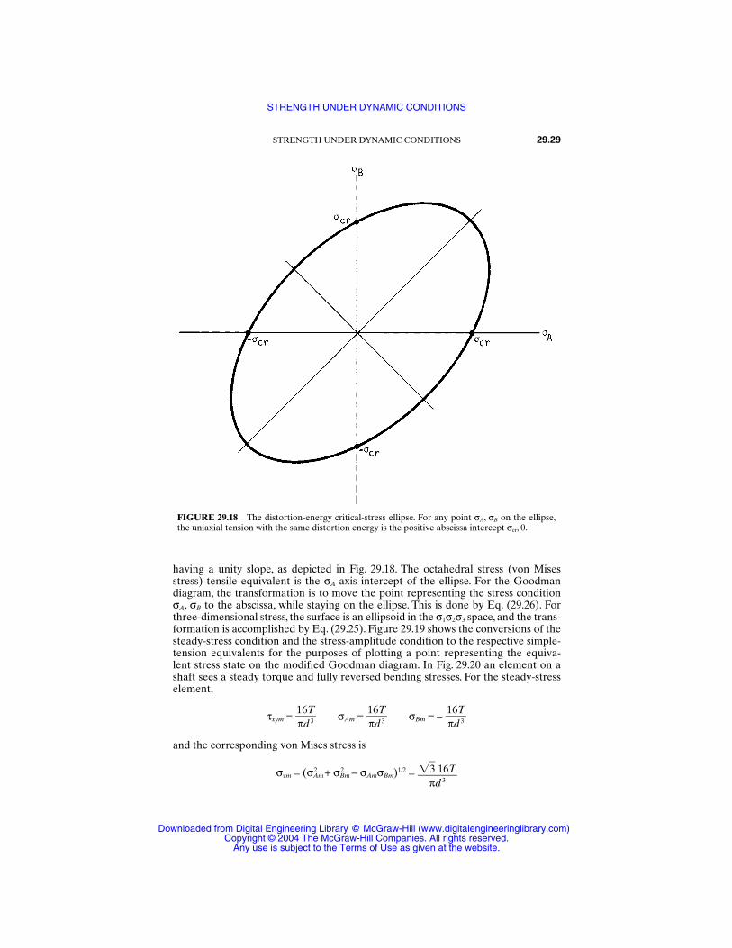
having a unity slope, as depicted in Fig. 29.18. The octahedral stress (von Misesstress) tensile equivalent is the σA-axis intercept of the ellipse. For the Goodman diagram, the transformation is to move the point representing the stress conditionσA, σB to the abscissa, while staying on the ellipse. This is done by Eq. (29.26). Forthree-dimensional stress, the surface is an ellipsoid in the σ1σ2σ3 space, and the trans-formation is accomplished by Eq. (29.25). Figure 29.19 shows the conversions of thesteady-stress condition and the stress-amplitude condition to the respective simple-tension equivalents for the purposes of plotting a point representing the equiva-lent stress state on the modified Goodman diagram. In Fig. 29.20 an element on ashaft sees a steady torque and fully reversed bending stresses. For the steady-stress element,
τxym = σAm = σBm = −
and the corresponding von Mises stress is
σvm = (σAm2 + σBm
2 − σAmσBm)1/2 = 3 16T
πd 3
16Tπd 3
16Tπd 3
16Tπd 3
STRENGTH UNDER DYNAMIC CONDITIONS 29.29
FIGURE 29.18 The distortion-energy critical-stress ellipse. For any point σA, σB on the ellipse,the uniaxial tension with the same distortion energy is the positive abscissa intercept σcr, 0.
STRENGTH UNDER DYNAMIC CONDITIONS
Downloaded from Digital Engineering Library @ McGraw-Hill (www.digitalengineeringlibrary.com)Copyright © 2004 The McGraw-Hill Companies. All rights reserved.
Any use is subject to the Terms of Use as given at the website.
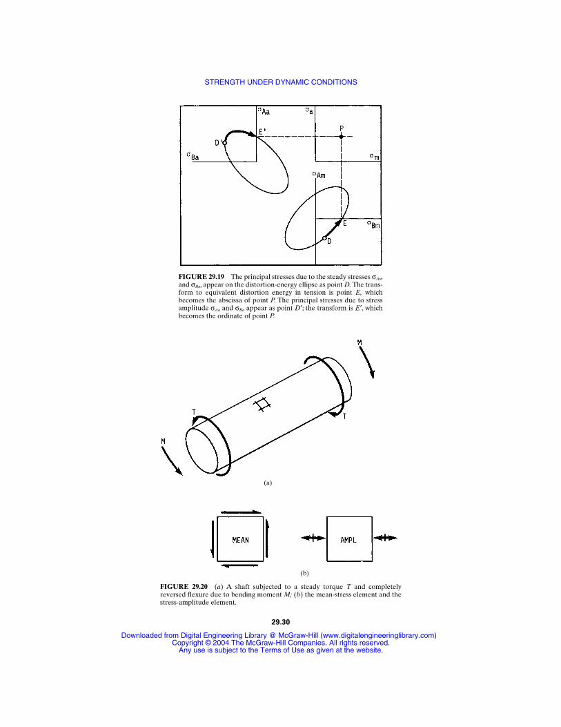
FIGURE 29.19 The principal stresses due to the steady stresses σAm
and σBm appear on the distortion-energy ellipse as point D. The trans-form to equivalent distortion energy in tension is point E, whichbecomes the abscissa of point P. The principal stresses due to stressamplitude σAa and σBa appear as point D′; the transform is E′, whichbecomes the ordinate of point P.
FIGURE 29.20 (a) A shaft subjected to a steady torque T and completelyreversed flexure due to bending moment M; (b) the mean-stress element and thestress-amplitude element.
(b)
(a)
29.30
STRENGTH UNDER DYNAMIC CONDITIONS
Downloaded from Digital Engineering Library @ McGraw-Hill (www.digitalengineeringlibrary.com)Copyright © 2004 The McGraw-Hill Companies. All rights reserved.
Any use is subject to the Terms of Use as given at the website.
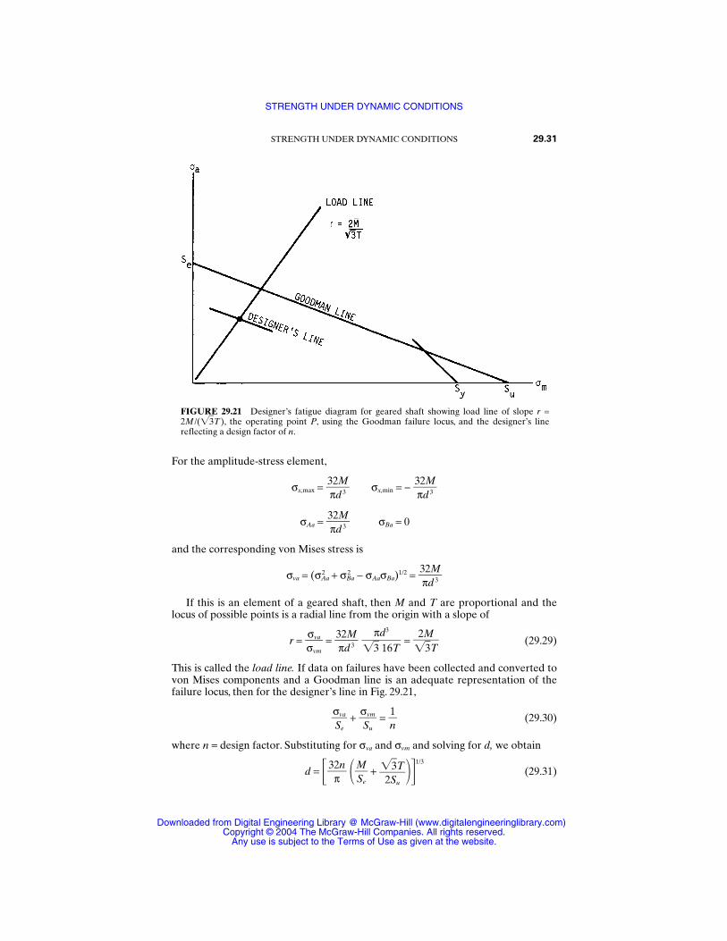
For the amplitude-stress element,
σx,max = σx,min = −
σAa = σBa = 0
and the corresponding von Mises stress is
σva = (σAa2 + σBa
2 − σAaσBa)1/2 =
If this is an element of a geared shaft, then M and T are proportional and thelocus of possible points is a radial line from the origin with a slope of
r = = = (29.29)
This is called the load line. If data on failures have been collected and converted tovon Mises components and a Goodman line is an adequate representation of thefailure locus, then for the designer’s line in Fig. 29.21,
+ = (29.30)
where n = design factor. Substituting for σva and σvm and solving for d, we obtain
d = + 1/3
(29.31)3T
2Su
MSe
32n
π
1n
σvmSu
σvaSe
2M3T
πd3
3 16T
32Mπd 3
σvaσvm
32Mπd 3
32Mπd 3
32Mπd 3
32Mπd 3
STRENGTH UNDER DYNAMIC CONDITIONS 29.31
FIGURE 29.21 Designer’s fatigue diagram for geared shaft showing load line of slope r =2M /(3T), the operating point P, using the Goodman failure locus, and the designer’s linereflecting a design factor of n.
STRENGTH UNDER DYNAMIC CONDITIONS
Downloaded from Digital Engineering Library @ McGraw-Hill (www.digitalengineeringlibrary.com)Copyright © 2004 The McGraw-Hill Companies. All rights reserved.
Any use is subject to the Terms of Use as given at the website.
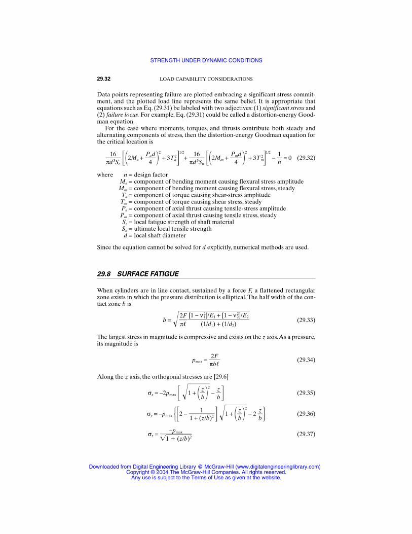
Data points representing failure are plotted embracing a significant stress commit-ment, and the plotted load line represents the same belief. It is appropriate thatequations such as Eq. (29.31) be labeled with two adjectives: (1) significant stress and(2) failure locus. For example, Eq. (29.31) could be called a distortion-energy Good-man equation.
For the case where moments, torques, and thrusts contribute both steady andalternating components of stress, then the distortion-energy Goodman equation forthe critical location is
2Ma + 2
+ 3Ta2
1/2
+ 2Mm + 2
+ 3Tm2
1/2
− = 0 (29.32)
where n = design factorMa = component of bending moment causing flexural stress amplitudeMm = component of bending moment causing flexural stress, steadyTa = component of torque causing shear-stress amplitudeTm = component of torque causing shear stress, steadyPa = component of axial thrust causing tensile-stress amplitudePm = component of axial thrust causing tensile stress, steadySe = local fatigue strength of shaft materialSu = ultimate local tensile strengthd = local shaft diameter
Since the equation cannot be solved for d explicitly, numerical methods are used.
29.8 SURFACE FATIGUE
When cylinders are in line contact, sustained by a force F, a flattened rectangularzone exists in which the pressure distribution is elliptical. The half width of the con-tact zone b is
b = (29.33)
The largest stress in magnitude is compressive and exists on the z axis.As a pressure,its magnitude is
pmax = (29.34)
Along the z axis, the orthogonal stresses are [29.6]
σx = −2pmax 1 + bz
2 −
bz
(29.35)
σy = −pmax 2 − 1 + bz
2 − 2
bz
(29.36)
σz = (29.37)−pmax
1 (z/b)2
11 + (z/b)2
2Fπb
[1 − ν 12]/E1 + [1 − ν2
2]/E2
(1/d1) + (1/d2)2Fπ
1n
Pmd
416
πd 3Su
Pad
416
πd 3Se
29.32 LOAD CAPABILITY CONSIDERATIONS
STRENGTH UNDER DYNAMIC CONDITIONS
Downloaded from Digital Engineering Library @ McGraw-Hill (www.digitalengineeringlibrary.com)Copyright © 2004 The McGraw-Hill Companies. All rights reserved.
Any use is subject to the Terms of Use as given at the website.
These equations can be useful with rolling contact, such as occurs in cams, rollerbearings, and gear teeth. The approach of the center of the rollers is
∆ = + ln + ln + (29.38)
The largest principal stress is compressive and located at the center of the rectangu-lar flat and is −pmax in magnitude. The largest shear stress is approximately 0.30pmax
and is located at about 0.78b below the surface. The maximum compressive stress isrepeatedly applied in rolling cylinders. At a position of z = 0.4b, y = 0.915b the shearstress has a magnitude of 0.242pmax but is completely reversed in rolling cylinders.
The loss of surface integrity due to repeated application of hertzian contactstresses is called surface fatigue. The phenomenon is marked by the loss of materialfrom the surface, leaving pits or voids. The onset of fatigue is often defined as theappearance of craters larger than a specified breadth. If Eq. (29.33) is substitutedinto Eq. (29.34) and the magnitude of pmax associated with the first tangible evidenceof fatigue at a specified number of cycles is called the surface endurance strength Sfe,then
F
d2
1 +
d2
2 = πSfe
2 + = K (29.39)
The left-hand side of the equation consists of parameters under the designer’s con-trol.The right-hand side consists of materials properties.The factor K is called Buck-ingham’s load-stress factor and is associated with a number of cycles. In gear studiesa similar K factor is used and is related to K through
Kg = K4 sin φ (29.40)
where φ = gear-tooth pressure angle. Note that pmax is proportional to other stressespresent, and it is conventional to describe surface fatigue in terms of the strength Sfe. Reference [29.1] gives Kg information for pressure angles of φ = 141⁄2 degrees andφ = 20 degrees, as well as Sfe for various materials and numbers of cycles. The impli-cation in the literature that above various cycles Kg does not change is unsupported.Log-log plots of K or Kg versus cycles to failure produce “parallel” lines with someconsistency in slope for classes of material.AGMA standard 218.01 (Dec. 1982) sug-gests allowable contact-stress numbers for steel as high as
(σ)107 = 0.364HB + 27 kpsi (29.41)
for 107 cycles, and for the curve fit for other than 107 cycles,
σN = CLσ107 = 2.46N −0.056(0.364HB + 27) kpsi (29.42)
For applications where little or no pitting is permissible, the slope of −0.056 persiststo 1010 (end of presentation). Another curve fit to Sfe data for steel at 108 cycles is
(Sfe)108 = 0.4HB − 10 kpsi (29.43)
When a gear and pinion are in mesh, the number of cycles to which a point on thetooth surface is exposed is different. Consequently, the material strengths can betuned to have both pinion and gear show tangible signs of wear simultaneously. Forsteel gears, using Eq. (29.43), the appropriate gear hardness BHN for a stipulatedpinion hardness bhn is
BHN = mGb/2(bhn − 25) + 25 (29.44)
1 − ν22
E2
1 − ν12
E1
23
d2b
d1b
1 − ν22
E2
1 − ν12
E1
2Fπ
STRENGTH UNDER DYNAMIC CONDITIONS 29.33
STRENGTH UNDER DYNAMIC CONDITIONS
Downloaded from Digital Engineering Library @ McGraw-Hill (www.digitalengineeringlibrary.com)Copyright © 2004 The McGraw-Hill Companies. All rights reserved.
Any use is subject to the Terms of Use as given at the website.
where mG = gear ratio, i.e., teeth on the gear per tooth on the pinion. This matchingcan be done by controlling surface hardness. Strength matching for bending resis-tance is accomplished by control of core properties.
When needle bearings are specified, the needle assembly is a vendor’s product,but the roller track is supplied by the user and is a design concern. The equivalentload Feq accumulating the same damage as a variable radial load F is
Feq = 2π
0F a dθ
1/a
If the entire assembly is vendor-supplied as a needle-bearing cam follower, then theaverage load is dictated by the cam-follower force F23. The follower makes m turnsper cam revolution. The follower’s first turn has an average load to the a power of
(F23)1a = 2π/m
0F 23
a dθ
where dθ = cam angular displacement. The subsequent averages are
(F23)2a = 4π/m
2π/mF 23
a dθ
⋅⋅⋅
The global average to the a power is
Fglobala =
m1
m
i = 1
(F23)ia =
21π 2π
0F23
a dθ
Consequently, the roller average radial load is identical to the cam’s, but the followermakes m times as many turns.
The follower contact surface between the cam and follower has an endurancestrength cycles-to-failure relation of the form of S−1/bN = K, and so the averagehertzian stress can be written
σH = 21π 2π
0σH
−1/b dθ−b
= 2π
0[F23(Kc + Kr)]−1/2b dθ
−b
(29.45)
where θ = cam rotation angle, b = slope of the rectified SN locus, w = width of theroller or cam (whichever is less), Cp = a joint materials constant
Cp = (29.46)
and the parameters Kc and Kr = the curvatures of the cam and roller surfaces, respec-tively.
One surface location on the cam sees the most intense hertzian stress every rev-olution. That spot has a hertzian stress of
σH = [F23(Kc + Kr)]max1/2 (29.47)
Cpw
1
π1 E−
1
ν12
+ 1
E−
2
ν22
12π
Cpw
12π/m
12π/m
12π
29.34 LOAD CAPABILITY CONSIDERATIONS
STRENGTH UNDER DYNAMIC CONDITIONS
Downloaded from Digital Engineering Library @ McGraw-Hill (www.digitalengineeringlibrary.com)Copyright © 2004 The McGraw-Hill Companies. All rights reserved.
Any use is subject to the Terms of Use as given at the website.
Relative strengths can be assessed by noting that the cam requires a strength of(Sfe)mN at the critical location in order to survive N cycles.The roller sees the averagestress everywhere on its periphery mN times, and its strength requirement is (Sfe)mN.The strength ratio is
=
=
If cam and roller are steel,
(Sfe)mN = mb(Sfe)N
enabling us to place endurance strengths on the same life basis, namely, N, which isconvenient when consulting tables of Buckingham load-strength data giving K or itsequivalent. Thus,
=
For steel, a 108 cycle expression, that is, (Sfe) = 0.4HB − 10 kpsi, can be used. Using bhnfor roller Brinell hardness and BHN for cam Brinell hardness, we can write
BHN = (bhn − 25) + 25 (29.48)
This form is convenient because the roller follower is often a vendor-supplied itemand the cam is manufactured elsewhere. Since max is larger than ()avg, thisalone tends to require that the cam be harder, but since the roller endures moreturns, the roller should be harder, since m > 1 and b < 0. Matching (tuning) therespective hardnesses so that the cam and roller will wear out together is often adesign goal.
Design factor can be introduced by reducing strength rather than increasing load(not equivalent when stress is not directly proportional to load). Since the loads areoften more accurately known than strengths in these applications, design factors are applied to strength. The relative hardnesses are unaffected by design factor, butthe necessary widths are
w = cam
2
max w = roller
2
()avgm−2b (29.49)
Either equation may be used. The width decision controls the median cycles to failure.
REFERENCES
29.1 R. C. Juvinall, Stress Strain and Strength, McGraw-Hill, New York, 1967, p. 218.
29.2 E. M. Prot, “Fatigue Testing under Progressive Loading: A New Technique for TestingMaterials,” E. J. Ward (trans.), Wright Air Development Center Tech. Rep., TR52-148,September 1952.
CpSfe/n
CpSfe/n
mb max
()avg
mb max
()avg
[(Sfe)N]cam[(Sfe)N]roller
max()avg
[F23(Kc + Kr)]max1/2
21π 2π
0[F23(Kc + Kr)]−1/2b dθ
−b
[(Sfe)N]cam[(Sfe)mN]roller
STRENGTH UNDER DYNAMIC CONDITIONS 29.35
STRENGTH UNDER DYNAMIC CONDITIONS
Downloaded from Digital Engineering Library @ McGraw-Hill (www.digitalengineeringlibrary.com)Copyright © 2004 The McGraw-Hill Companies. All rights reserved.
Any use is subject to the Terms of Use as given at the website.

29.3 J. A. Collins, Failure of Materials in Mechanical Design, Wiley-Interscience, New York,1981, chap. 10.
29.4 W. J. Dixon and F. J. Massey, Jr., Introduction to Statistical Analysis, 3d ed., McGraw-Hill,New York, 1969, p. 380.
29.5 J. T. Ransom, Statistical Aspects of Fatigue, Special Technical Publication No. 121, Amer-ican Society for Testing Materials, Philadelphia, Pa., 1952, p. 61.
29.6 J. E. Shigley and C. R. Mischke, Mechanical Engineering Design, 5th ed., McGraw-Hill,New York, 1989.
29.7 C. R. Mischke, “A Probabilistic Model of Size Effect in Fatigue Strength of Rounds inBending and Torsion,” Transactions of ASME, Journal of Machine Design, vol. 102, no. 1,January 1980, pp. 32–37.
29.8 C. R. Mischke, “A Rationale for Mechanical Design to a Reliability Specification,” Pro-ceedings of the Design Engineering Technical Conference of ASME, American Society ofMechanical Engineers, New York, 1974, pp. 221–248.
29.9 L. Sors, Fatigue Design of Machine Components, Part 1, Pergamon Press, Oxford, 1971,pp. 9–13.
29.10 H. J. Grover, S.A. Gordon, and L. R. Jackson, Fatigue of Metals and Structures, Bureau ofNaval Weapons Document NAVWEPS 00-25-534, Washington, D.C., 1960, pp. 282–314.
29.11 C. Lipson and R. C. Juvinall, Handbook of Stress and Strength, Macmillan, New York,1963.
29.12 R. C. Juvinall, Fundamentals of Machine Component Design, John Wiley & Sons,New York, 1983.
29.13 A. D. Deutschman, W. J. Michels, and C. E. Wilson, Machine Design, MacMillan,New York, 1975.
29.14 E. B. Haugen, Probabilistic Mechanical Design, John Wiley & Sons, New York, 1980.
29.15 C. R. Mischke, Mathematical Model Building, 2d rev. ed., Iowa State University Press,Ames, 1980.
29.16 G. Sines and J. L. Waisman (eds.), Metal Fatigue, McGraw-Hill, New York, 1959.
29.17 H. O. Fuchs and R. I. Stephens, Metal Fatigue in Engineering, John Wiley & Sons,New York, 1980.
RECOMMENDED READING
Proceedings of the Society of Automotive Engineers Fatigue Conference, P109, Warrendale, Pa.April 1982.
29.36 LOAD CAPABILITY CONSIDERATIONS
STRENGTH UNDER DYNAMIC CONDITIONS
Downloaded from Digital Engineering Library @ McGraw-Hill (www.digitalengineeringlibrary.com)Copyright © 2004 The McGraw-Hill Companies. All rights reserved.
Any use is subject to the Terms of Use as given at the website.

CHAPTER 30INSTABILITIES IN BEAMS
AND COLUMNS
Harry HermanProfessor of Mechanical Engineering
New Jersey Institute of TechnologyNewark, New Jersey
30.1 EULER’S FORMULA / 30.2
30.2 EFFECTIVE LENGTH / 30.4
30.3 GENERALIZATION OF THE PROBLEM / 30.6
30.4 MODIFIED BUCKLING FORMULAS / 30.7
30.5 STRESS-LIMITING CRITERION / 30.8
30.6 BEAM-COLUMN ANALYSIS / 30.12
30.7 APPROXIMATE METHOD / 30.13
30.8 INSTABILITY OF BEAMS / 30.14
REFERENCES / 30.18
NOTATION
A Area of cross sectionB(n) Arbitrary constantsc(n) Coefficients in seriesc(y), c(z) Distance from y and z axis, respectively, to outermost compressive
fibere Eccentricity of axial load PE Modulus of elasticity of materialE(t) Tangent modulus for buckling outside of elastic rangeF(x) A function of xG Shear modulus of materialh Height of cross sectionH Horizontal (transverse) force on columnI Moment of inertia of cross sectionI(y), I(z) Moment of inertia with respect to y and z axis, respectivelyJ Torsion constant; polar moment of inertiak2 P/EIK Effective-length coefficientK(0) Spring constant for constraining spring at origin
30.1
Source: STANDARD HANDBOOK OF MACHINE DESIGN
Downloaded from Digital Engineering Library @ McGraw-Hill (www.digitalengineeringlibrary.com)Copyright © 2004 The McGraw-Hill Companies. All rights reserved.
Any use is subject to the Terms of Use as given at the website.

K(T, 0), K(T, L) Torsional spring constants at x = 0, L, respectivelyl Developed length of cross sectionL Length of column or beamLeff Effective length of columnM, M′ Bending momentsM(0), M(L), Mmid Bending moments at x = 0, L, and midpoint, respectivelyM(0)cr Critical moment for buckling of beamMtr Moment due to transverse loadM(y), M(z) Moment about y and z axis, respectivelyn Integer; running indexP Axial load on columnPcr Critical axial load for buckling of columnr Radius of gyrationR Radius of cross sections Running coordinate, measured from one endt Thickness of cross sectionT Torque about x axisx Axial coordinate of column or beamy, z Transverse coordinates and deflectionsY Initial deflection (crookedness) of columnYtr Deflection of beam-column due to transverse loadη Factor of safetyσ Stressφ Angle of twist
As the terms beam and column imply, this chapter deals with members whose cross-sectional dimensions are small in comparison with their lengths. Particularly, we areconcerned with the stability of beams and columns whose axes in the undeformedstate are substantially straight. Classically, instability is associated with a state inwhich the deformation of an idealized, perfectly straight member can become arbi-trarily large. However, some of the criteria for stable design which we will developwill take into account the influences of imperfections such as the eccentricity of theaxial load and the crookedness of the centroidal axis of the column.The magnitudesof these imperfections are generally not known, but they can be estimated frommanufacturing tolerances. For axially loaded columns, the onset of instability isrelated to the moment of inertia of the column cross section about its minor princi-pal axis. For beams, stability design requires, in addition to the moment of inertia, theconsideration of the torsional stiffness.
30.1 EULER’S FORMULA
We will begin with the familiar Euler column-buckling problem.The column is ideal-ized as shown in Fig. 30.1. The top and bottom ends are pinned; that is, the moments
30.2 LOAD CAPABILITY CONSIDERATIONS
INSTABILITIES IN BEAMS AND COLUMNS
Downloaded from Digital Engineering Library @ McGraw-Hill (www.digitalengineeringlibrary.com)Copyright © 2004 The McGraw-Hill Companies. All rights reserved.
Any use is subject to the Terms of Use as given at the website.
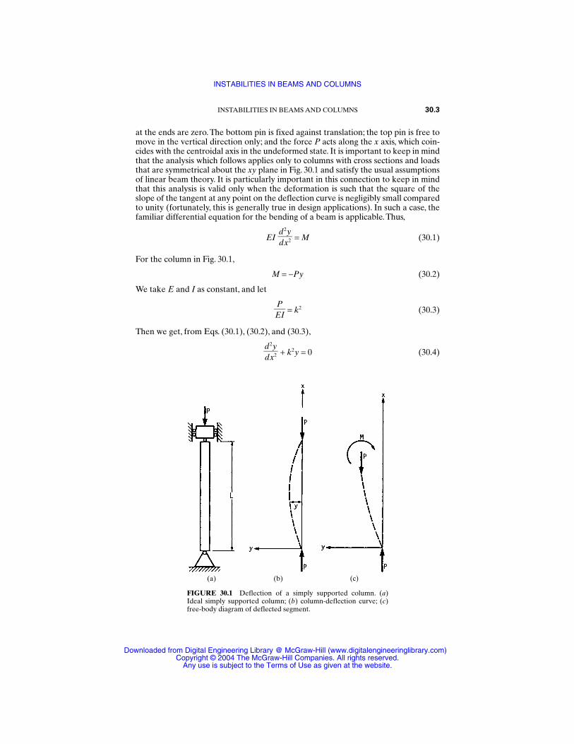
at the ends are zero. The bottom pin is fixed against translation; the top pin is free tomove in the vertical direction only; and the force P acts along the x axis, which coin-cides with the centroidal axis in the undeformed state. It is important to keep in mindthat the analysis which follows applies only to columns with cross sections and loadsthat are symmetrical about the xy plane in Fig. 30.1 and satisfy the usual assumptionsof linear beam theory. It is particularly important in this connection to keep in mindthat this analysis is valid only when the deformation is such that the square of theslope of the tangent at any point on the deflection curve is negligibly small comparedto unity (fortunately, this is generally true in design applications). In such a case, thefamiliar differential equation for the bending of a beam is applicable. Thus,
EI = M (30.1)
For the column in Fig. 30.1,
M = −Py (30.2)
We take E and I as constant, and let
EPI = k2 (30.3)
Then we get, from Eqs. (30.1), (30.2), and (30.3),
+ k2y = 0 (30.4)d2ydx2
d2ydx2
INSTABILITIES IN BEAMS AND COLUMNS 30.3
FIGURE 30.1 Deflection of a simply supported column. (a)Ideal simply supported column; (b) column-deflection curve; (c)free-body diagram of deflected segment.
(a) (b) (c)
INSTABILITIES IN BEAMS AND COLUMNS
Downloaded from Digital Engineering Library @ McGraw-Hill (www.digitalengineeringlibrary.com)Copyright © 2004 The McGraw-Hill Companies. All rights reserved.
Any use is subject to the Terms of Use as given at the website.
The boundary conditions at x = 0 and x = L are
y(0) = y(L) = 0 (30.5)
In order that Eqs. (30.4) and (30.5) should have a solution y(x) that need not beequal to zero for all values of x, k must take one of the values in Eq. (30.6):
k(n) = nLπ n = 1, 2, 3, . . . (30.6)
which means that the axial load P must take one of the values in Eq. (30.7):
P(n) = n = 1, 2, 3, . . . (30.7)
For each value of n, the corresponding nonzero solution for y is
y(n) = B(n) sin n = 1, 2, 3, . . . (30.8)
where B(n) is an arbitrary constant.In words, the preceding results state the following: Suppose that we have a per-
fectly straight prismatic column with constant properties over its entire length. If thecolumn is subjected to a perfectly axial load, there is a set of load values, togetherwith a set of sine-shaped deformation curves for the column axis, such that theapplied moment due to the axial load and the resisting internal moment are in equi-librium everywhere along the column, no matter what the amplitude of the sinecurve may be. From Eq. (30.7), the smallest load at which such deformation occurs,called the critical load, is
Pcr = (30.9)
This is the familiar Euler formula.
30.2 EFFECTIVE LENGTH
Note that the sinusoidal shape of the solution function is determined by the differ-ential equation and does not depend on the boundary conditions. If we can find asegment of a sinusoidal curve that satisfies our chosen boundary conditions and, inturn, we can find some segment of that curve which matches the curve in Fig. 30.1,we can establish a correlation between the two cases. This notion is the basis for the“effective-length” concept. Recall that Eq. (30.9) was obtained for a column withboth ends simply supported (that is, the moment is zero at the ends). Figure 30.2illustrates columns of length L with various idealized end conditions. In each case,there is a multiple of L, KL, which is called the effective length of the column Leff,that has a shape which is similar to and behaves like a simply supported column ofthat length. To determine the critical loads for columns whose end supports may beidealized as shown in Fig. 30.2, we can make use of Eq. (30.9) if we replace L by KL,with the appropriate value of K taken from Fig. 30.2. Particular care has to be taken
π2EI
L2
nπx
L
n2π2EI
L2
30.4 LOAD CAPABILITY CONSIDERATIONS
INSTABILITIES IN BEAMS AND COLUMNS
Downloaded from Digital Engineering Library @ McGraw-Hill (www.digitalengineeringlibrary.com)Copyright © 2004 The McGraw-Hill Companies. All rights reserved.
Any use is subject to the Terms of Use as given at the website.
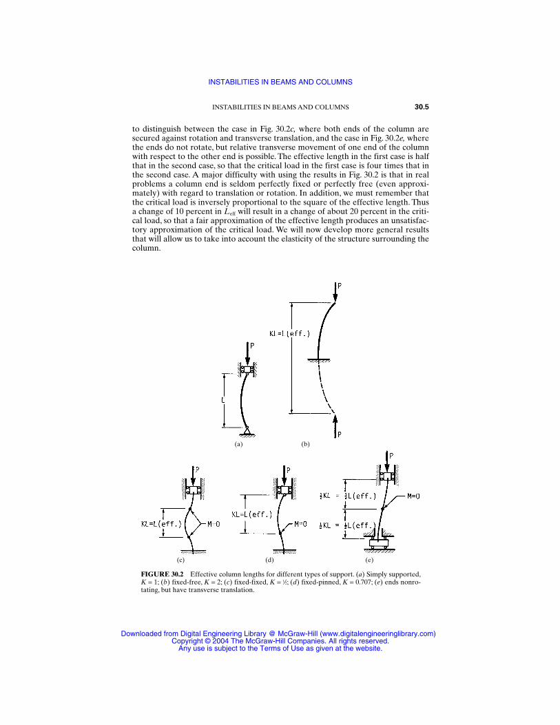
to distinguish between the case in Fig. 30.2c, where both ends of the column aresecured against rotation and transverse translation, and the case in Fig. 30.2e, wherethe ends do not rotate, but relative transverse movement of one end of the columnwith respect to the other end is possible. The effective length in the first case is halfthat in the second case, so that the critical load in the first case is four times that inthe second case. A major difficulty with using the results in Fig. 30.2 is that in realproblems a column end is seldom perfectly fixed or perfectly free (even approxi-mately) with regard to translation or rotation. In addition, we must remember thatthe critical load is inversely proportional to the square of the effective length. Thusa change of 10 percent in Leff will result in a change of about 20 percent in the criti-cal load, so that a fair approximation of the effective length produces an unsatisfac-tory approximation of the critical load. We will now develop more general resultsthat will allow us to take into account the elasticity of the structure surrounding thecolumn.
INSTABILITIES IN BEAMS AND COLUMNS 30.5
FIGURE 30.2 Effective column lengths for different types of support. (a) Simply supported,K = 1; (b) fixed-free, K = 2; (c) fixed-fixed, K = 1⁄2; (d) fixed-pinned, K = 0.707; (e) ends nonro-tating, but have transverse translation.
(a) (b)
(c) (d) (e)
INSTABILITIES IN BEAMS AND COLUMNS
Downloaded from Digital Engineering Library @ McGraw-Hill (www.digitalengineeringlibrary.com)Copyright © 2004 The McGraw-Hill Companies. All rights reserved.
Any use is subject to the Terms of Use as given at the website.
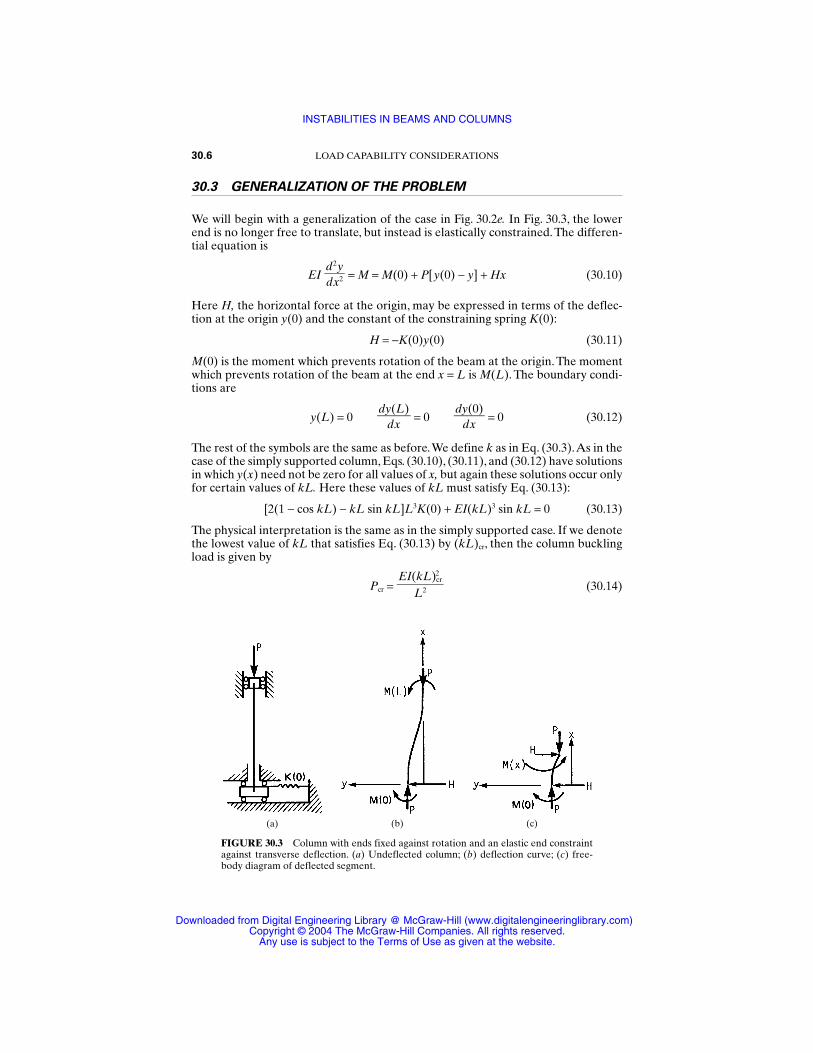
30.3 GENERALIZATION OF THE PROBLEM
We will begin with a generalization of the case in Fig. 30.2e. In Fig. 30.3, the lowerend is no longer free to translate, but instead is elastically constrained. The differen-tial equation is
EI = M = M(0) + P[y(0) − y] + Hx (30.10)
Here H, the horizontal force at the origin, may be expressed in terms of the deflec-tion at the origin y(0) and the constant of the constraining spring K(0):
H = −K(0)y(0) (30.11)
M(0) is the moment which prevents rotation of the beam at the origin. The momentwhich prevents rotation of the beam at the end x = L is M(L). The boundary condi-tions are
y(L) = 0 = 0 = 0 (30.12)
The rest of the symbols are the same as before.We define k as in Eq. (30.3).As in thecase of the simply supported column, Eqs. (30.10), (30.11), and (30.12) have solutionsin which y(x) need not be zero for all values of x, but again these solutions occur onlyfor certain values of kL. Here these values of kL must satisfy Eq. (30.13):
[2(1 − cos kL) − kL sin kL]L3K(0) + EI(kL)3 sin kL = 0 (30.13)
The physical interpretation is the same as in the simply supported case. If we denotethe lowest value of kL that satisfies Eq. (30.13) by (kL)cr, then the column bucklingload is given by
Pcr = (30.14)EI(kL)2
cr
L2
dy(0)
dxdy(L)
dx
d2ydx2
30.6 LOAD CAPABILITY CONSIDERATIONS
FIGURE 30.3 Column with ends fixed against rotation and an elastic end constraintagainst transverse deflection. (a) Undeflected column; (b) deflection curve; (c) free-body diagram of deflected segment.
(a) (b) (c)
INSTABILITIES IN BEAMS AND COLUMNS
Downloaded from Digital Engineering Library @ McGraw-Hill (www.digitalengineeringlibrary.com)Copyright © 2004 The McGraw-Hill Companies. All rights reserved.
Any use is subject to the Terms of Use as given at the website.
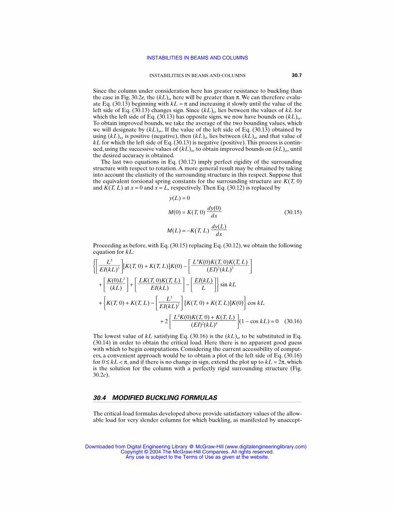
Since the column under consideration here has greater resistance to buckling thanthe case in Fig. 30.2e, the (kL)cr here will be greater than π. We can therefore evalu-ate Eq. (30.13) beginning with kL = π and increasing it slowly until the value of theleft side of Eq. (30.13) changes sign. Since (kL)cr lies between the values of kL forwhich the left side of Eq. (30.13) has opposite signs, we now have bounds on (kL)cr.To obtain improved bounds, we take the average of the two bounding values, whichwe will designate by (kL)av. If the value of the left side of Eq. (30.13) obtained byusing (kL)av is positive (negative), then (kL)cr lies between (kL)av and that value ofkL for which the left side of Eq. (30.13) is negative (positive).This process is contin-ued, using the successive values of (kL)av to obtain improved bounds on (kL)cr, untilthe desired accuracy is obtained.
The last two equations in Eq. (30.12) imply perfect rigidity of the surroundingstructure with respect to rotation. A more general result may be obtained by takinginto account the elasticity of the surrounding structure in this respect. Suppose thatthe equivalent torsional spring constants for the surrounding structure are K(T, 0)and K(T, L) at x = 0 and x = L, respectively. Then Eq. (30.12) is replaced by
y(L) = 0
M(0) = K(T, 0) (30.15)
M(L) = −K(T, L)
Proceeding as before, with Eq. (30.15) replacing Eq. (30.12), we obtain the followingequation for kL:
[K(T, 0) + K(T, L)]K(0) − + + − sin kL
+ K(T, 0) + K(T, L) − [K(T, 0) + K(T, L)]K(0) cos kL
+ 2 (1 − cos kL) = 0 (30.16)
The lowest value of kL satisfying Eq. (30.16) is the (kL)cr to be substituted in Eq.(30.14) in order to obtain the critical load. Here there is no apparent good guesswith which to begin computations. Considering the current accessibility of comput-ers, a convenient approach would be to obtain a plot of the left side of Eq. (30.16)for 0 ≤ kL < π, and if there is no change in sign, extend the plot up to kL = 2π, whichis the solution for the column with a perfectly rigid surrounding structure (Fig.30.2c).
30.4 MODIFIED BUCKLING FORMULAS
The critical-load formulas developed above provide satisfactory values of the allow-able load for very slender columns for which buckling, as manifested by unaccept-
L4K(0)K(T, 0) + K(T, L)
(EI)2(kL)4
L3
EI(kL)2
EI(kL)
LLK(T, 0)K(T, L)
EI(kL)K(0)L2
(kL)
L4K(0)K(T, 0)K(T, L)
(EI)2(kL)3
L3
EI(kL)3
dy(L)
dx
dy(0)
dx
INSTABILITIES IN BEAMS AND COLUMNS 30.7
INSTABILITIES IN BEAMS AND COLUMNS
Downloaded from Digital Engineering Library @ McGraw-Hill (www.digitalengineeringlibrary.com)Copyright © 2004 The McGraw-Hill Companies. All rights reserved.
Any use is subject to the Terms of Use as given at the website.
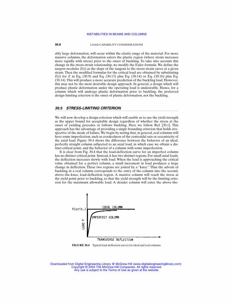
ably large deformation, will occur within the elastic range of the material. For moremassive columns, the deformation enters the plastic region (where strain increasesmore rapidly with stress) prior to the onset of buckling. To take into account thischange in the stress-strain relationship, we modify the Euler formula. We define thetangent modulus E(t) as the slope of the tangent to the stress-strain curve at a givenstrain. Then the modified formulas for the critical load are obtained by substitutingE(t) for E in Eq. (30.9) and Eq. (30.13) plus Eq. (30.14) or Eq. (30.16) plus Eq.(30.14).This will produce a more accurate prediction of the buckling load. However,this may not be the most desirable design approach. In general, a design which willproduce plastic deformation under the operating load is undesirable. Hence, for acolumn which will undergo plastic deformation prior to buckling, the preferreddesign-limiting criterion is the onset of plastic deformation, not the buckling.
30.5 STRESS-LIMITING CRITERION
We will now develop a design criterion which will enable us to use the yield strengthas the upper bound for acceptable design regardless of whether the stress at theonset of yielding precedes or follows buckling. Here we follow Ref. [30.1]. Thisapproach has the advantage of providing a single bounding criterion that holds irre-spective of the mode of failure.We begin by noting that, in general, real columns willhave some imperfection, such as crookedness of the centroidal axis or eccentricity ofthe axial load. Figure 30.4 shows the difference between the behavior of an ideal,perfectly straight column subjected to an axial load, in which case we obtain a dis-tinct critical point, and the behavior of a column with some imperfection.
It is clear from Fig. 30.4 that the load-deflection curve for an imperfect columnhas no distinct critical point. Instead, it has two distinct regions. For small axial loads,the deflection increases slowly with load. When the load is approaching the criticalvalue obtained for a perfect column, a small increment in load produces a largechange in deflection. These two regions are joined by a “knee.” Thus the advent ofbuckling in a real column corresponds to the entry of the column into the second,above-the-knee, load-deflection region. A massive column will reach the stress atthe yield point prior to buckling, so that the yield strength will be the limiting crite-rion for the maximum allowable load. A slender column will enter the above-the-
30.8 LOAD CAPABILITY CONSIDERATIONS
FIGURE 30.4 Typical load-deflection curves for ideal and real columns.
INSTABILITIES IN BEAMS AND COLUMNS
Downloaded from Digital Engineering Library @ McGraw-Hill (www.digitalengineeringlibrary.com)Copyright © 2004 The McGraw-Hill Companies. All rights reserved.
Any use is subject to the Terms of Use as given at the website.
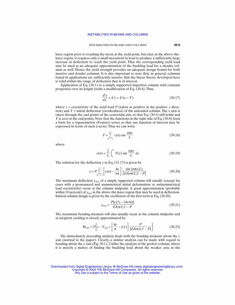
knee region prior to reaching the stress at the yield point, but once in the above-the-knee region, it requires only a small increment in load to produce a sufficiently largeincrease in deflection to reach the yield point. Thus the corresponding yield loadmay be used as an adequate approximation of the buckling load for a slender col-umn as well. Hence the yield strength provides an adequate design bound for bothmassive and slender columns. It is also important to note that, in general, columnsfound in applications are sufficiently massive that the linear theory developed hereis valid within the range of deflection that is of interest.
Application of Eq. (30.1) to a simply supported imperfect column with constantproperties over its length yields a modification of Eq. (30.4). Thus,
+ k2y = k2(e − Y) (30.17)
where e = eccentricity of the axial load P (taken as positive in the positive y direc-tion) and Y = initial deflection (crookedness) of the unloaded column. The x axis istaken through the end points of the centroidal axis, so that Eq. (30.5) still holds andY is zero at the end points. Note that the functions in the right side of Eq. (30.8) forma basis for a trigonometric (Fourier) series, so that any function of interest may beexpressed in terms of such a series. Thus we can write
Y = ∞
n = 1
c(n) sin (30.18)
where
c(n) = L2
L
0Y(x) sin dx (30.19)
The solution for the deflection y in Eq. (15.17) is given by
y = P ∞
n = 1c(n) − (30.20)
The maximum deflection ymax of a simply supported column will usually (except forcases with a pronounced and asymmetrical initial deformation or antisymmetricalload eccentricity) occur at the column midpoint. A good approximation (probablywithin 10 percent) of ymax in the above-the-knee region that may be used in deflection-limited column design is given by the coefficient of the first term in Eq. (30.20):
ymax = (30.21)
The maximum bending moment will also usually occur at the column midpoint andat incipient yielding is closely approximated by
Mmax = Pe − Ymid + 4πe − c(1) (30.22)
The immediately preceding analysis deals with the bending moment about the zaxis (normal to the paper). Clearly, a similar analysis can be made with regard tobending about the y axis (Fig. 30.1). Unlike the analysis of the perfect column, whereit is merely a matter of finding the buckling load about the weaker axis, in the
P[EI(π/L)2 − P]
P[c(1) − (4e/π)]
EI(π/L)2 − P
sin (nπx/L)[EI(nπ/L)2 − P]
4enπ
nπx
L
nπx
L
d2ydx2
INSTABILITIES IN BEAMS AND COLUMNS 30.9
INSTABILITIES IN BEAMS AND COLUMNS
Downloaded from Digital Engineering Library @ McGraw-Hill (www.digitalengineeringlibrary.com)Copyright © 2004 The McGraw-Hill Companies. All rights reserved.
Any use is subject to the Terms of Use as given at the website.
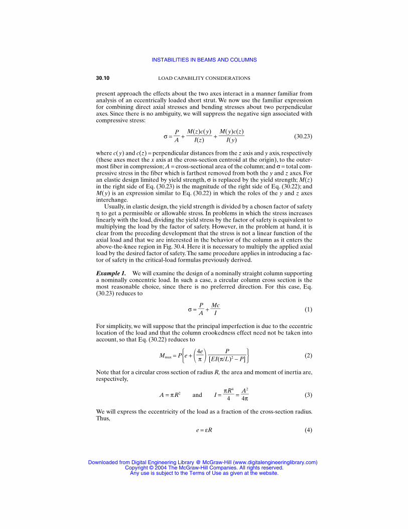
present approach the effects about the two axes interact in a manner familiar fromanalysis of an eccentrically loaded short strut. We now use the familiar expressionfor combining direct axial stresses and bending stresses about two perpendicularaxes. Since there is no ambiguity, we will suppress the negative sign associated withcompressive stress:
σ = AP
+ + (30.23)
where c(y) and c(z) = perpendicular distances from the z axis and y axis, respectively(these axes meet the x axis at the cross-section centroid at the origin), to the outer-most fiber in compression; A = cross-sectional area of the column; and σ = total com-pressive stress in the fiber which is farthest removed from both the y and z axes. Foran elastic design limited by yield strength, σ is replaced by the yield strength; M(z)in the right side of Eq. (30.23) is the magnitude of the right side of Eq. (30.22); andM(y) is an expression similar to Eq. (30.22) in which the roles of the y and z axesinterchange.
Usually, in elastic design, the yield strength is divided by a chosen factor of safetyη to get a permissible or allowable stress. In problems in which the stress increaseslinearly with the load, dividing the yield stress by the factor of safety is equivalent tomultiplying the load by the factor of safety. However, in the problem at hand, it isclear from the preceding development that the stress is not a linear function of theaxial load and that we are interested in the behavior of the column as it enters theabove-the-knee region in Fig. 30.4. Here it is necessary to multiply the applied axialload by the desired factor of safety.The same procedure applies in introducing a fac-tor of safety in the critical-load formulas previously derived.
Example 1. We will examine the design of a nominally straight column supportinga nominally concentric load. In such a case, a circular column cross section is themost reasonable choice, since there is no preferred direction. For this case, Eq.(30.23) reduces to
σ = AP
+ MIc
(1)
For simplicity, we will suppose that the principal imperfection is due to the eccentriclocation of the load and that the column crookedness effect need not be taken intoaccount, so that Eq. (30.22) reduces to
Mmax = Pe + 4πe (2)
Note that for a circular cross section of radius R, the area and moment of inertia are,respectively,
A = πR2 and I = = (3)
We will express the eccentricity of the load as a fraction of the cross-section radius.Thus,
e = εR (4)
A2
4π
πR4
4
P[EI(π/L)2 − P]
M(y)c(z)
I(y)M(z)c(y)
I(z)
30.10 LOAD CAPABILITY CONSIDERATIONS
INSTABILITIES IN BEAMS AND COLUMNS
Downloaded from Digital Engineering Library @ McGraw-Hill (www.digitalengineeringlibrary.com)Copyright © 2004 The McGraw-Hill Companies. All rights reserved.
Any use is subject to the Terms of Use as given at the website.
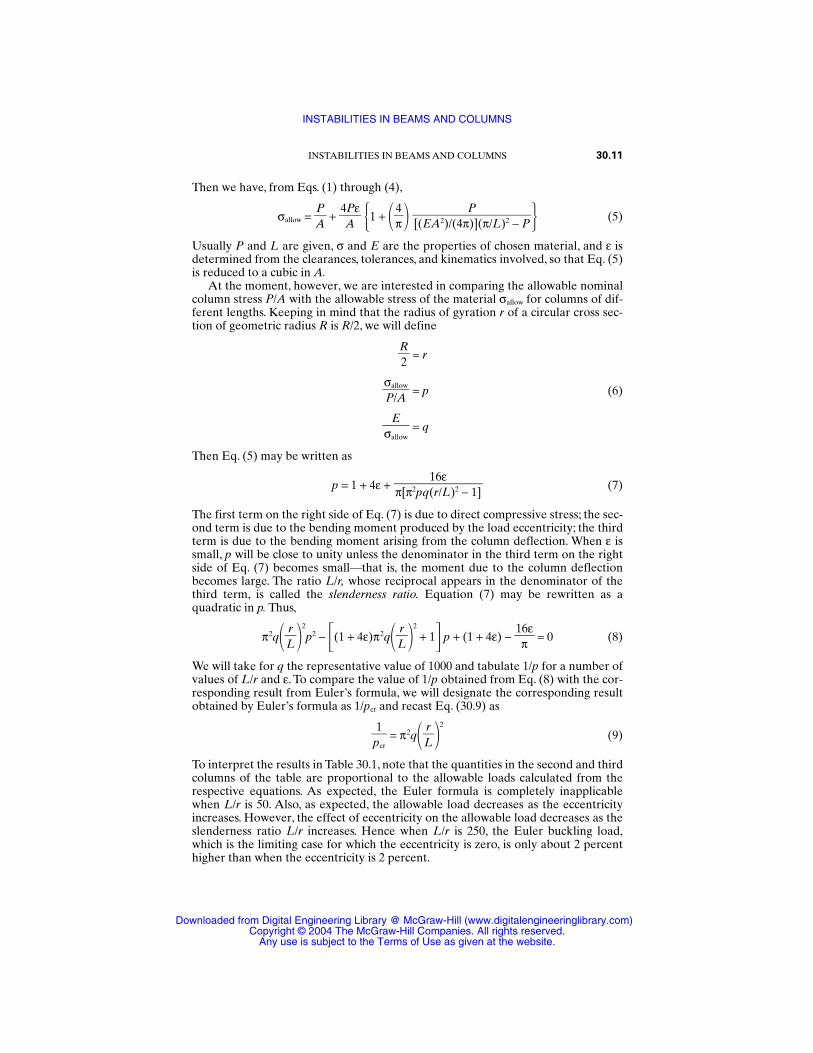
Then we have, from Eqs. (1) through (4),
σallow = AP
+ 4APε 1 +
π4
(5)
Usually P and L are given, σ and E are the properties of chosen material, and ε isdetermined from the clearances, tolerances, and kinematics involved, so that Eq. (5)is reduced to a cubic in A.
At the moment, however, we are interested in comparing the allowable nominalcolumn stress P/A with the allowable stress of the material σallow for columns of dif-ferent lengths. Keeping in mind that the radius of gyration r of a circular cross sec-tion of geometric radius R is R/2, we will define
R2
= r
= p (6)
= q
Then Eq. (5) may be written as
p = 1 + 4ε + (7)
The first term on the right side of Eq. (7) is due to direct compressive stress; the sec-ond term is due to the bending moment produced by the load eccentricity; the thirdterm is due to the bending moment arising from the column deflection. When ε issmall, p will be close to unity unless the denominator in the third term on the rightside of Eq. (7) becomes small—that is, the moment due to the column deflectionbecomes large. The ratio L/r, whose reciprocal appears in the denominator of thethird term, is called the slenderness ratio. Equation (7) may be rewritten as aquadratic in p. Thus,
π2qLr
2
p2 − (1 + 4ε)π2qLr
2
+ 1 p + (1 + 4ε) − 1π6ε = 0 (8)
We will take for q the representative value of 1000 and tabulate 1/p for a number ofvalues of L/r and ε. To compare the value of 1/p obtained from Eq. (8) with the cor-responding result from Euler’s formula, we will designate the corresponding resultobtained by Euler’s formula as 1/pcr and recast Eq. (30.9) as
p1cr = π2q
Lr
2
(9)
To interpret the results in Table 30.1, note that the quantities in the second and thirdcolumns of the table are proportional to the allowable loads calculated from therespective equations. As expected, the Euler formula is completely inapplicablewhen L/r is 50. Also, as expected, the allowable load decreases as the eccentricityincreases. However, the effect of eccentricity on the allowable load decreases as theslenderness ratio L/r increases. Hence when L/r is 250, the Euler buckling load,which is the limiting case for which the eccentricity is zero, is only about 2 percenthigher than when the eccentricity is 2 percent.
16επ[π2pq(r/L)2 − 1]
Eσallow
σallowP/A
P[(EA2)/(4π)](π/L)2 − P
INSTABILITIES IN BEAMS AND COLUMNS 30.11
INSTABILITIES IN BEAMS AND COLUMNS
Downloaded from Digital Engineering Library @ McGraw-Hill (www.digitalengineeringlibrary.com)Copyright © 2004 The McGraw-Hill Companies. All rights reserved.
Any use is subject to the Terms of Use as given at the website.
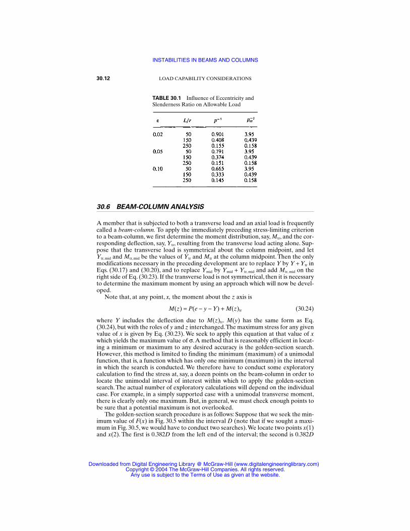
30.6 BEAM-COLUMN ANALYSIS
A member that is subjected to both a transverse load and an axial load is frequentlycalled a beam-column. To apply the immediately preceding stress-limiting criterionto a beam-column, we first determine the moment distribution, say, Mtr, and the cor-responding deflection, say, Ytr, resulting from the transverse load acting alone. Sup-pose that the transverse load is symmetrical about the column midpoint, and let Ytr, mid and Mtr, mid be the values of Ytr and Mtr at the column midpoint. Then the onlymodifications necessary in the preceding development are to replace Y by Y + Ytr inEqs. (30.17) and (30.20), and to replace Ymid by Ymid + Ytr, mid and add Mtr, mid on theright side of Eq. (30.23). If the transverse load is not symmetrical, then it is necessaryto determine the maximum moment by using an approach which will now be devel-oped.
Note that, at any point, x, the moment about the z axis is
M(z) = P(e − y − Y) + M(z)tr (30.24)
where Y includes the deflection due to M(z)tr. M(y) has the same form as Eq.(30.24), but with the roles of y and z interchanged.The maximum stress for any givenvalue of x is given by Eq. (30.23). We seek to apply this equation at that value of xwhich yields the maximum value of σ.A method that is reasonably efficient in locat-ing a minimum or maximum to any desired accuracy is the golden-section search.However, this method is limited to finding the minimum (maximum) of a unimodalfunction, that is, a function which has only one minimum (maximum) in the intervalin which the search is conducted. We therefore have to conduct some exploratorycalculation to find the stress at, say, a dozen points on the beam-column in order tolocate the unimodal interval of interest within which to apply the golden-sectionsearch. The actual number of exploratory calculations will depend on the individualcase. For example, in a simply supported case with a unimodal transverse moment,there is clearly only one maximum. But, in general, we must check enough points tobe sure that a potential maximum is not overlooked.
The golden-section search procedure is as follows: Suppose that we seek the min-imum value of F(x) in Fig. 30.5 within the interval D (note that if we sought a maxi-mum in Fig. 30.5, we would have to conduct two searches).We locate two points x(1)and x(2). The first is 0.382D from the left end of the interval; the second is 0.382D
30.12 LOAD CAPABILITY CONSIDERATIONS
TABLE 30.1 Influence of Eccentricity andSlenderness Ratio on Allowable Load
INSTABILITIES IN BEAMS AND COLUMNS
Downloaded from Digital Engineering Library @ McGraw-Hill (www.digitalengineeringlibrary.com)Copyright © 2004 The McGraw-Hill Companies. All rights reserved.
Any use is subject to the Terms of Use as given at the website.
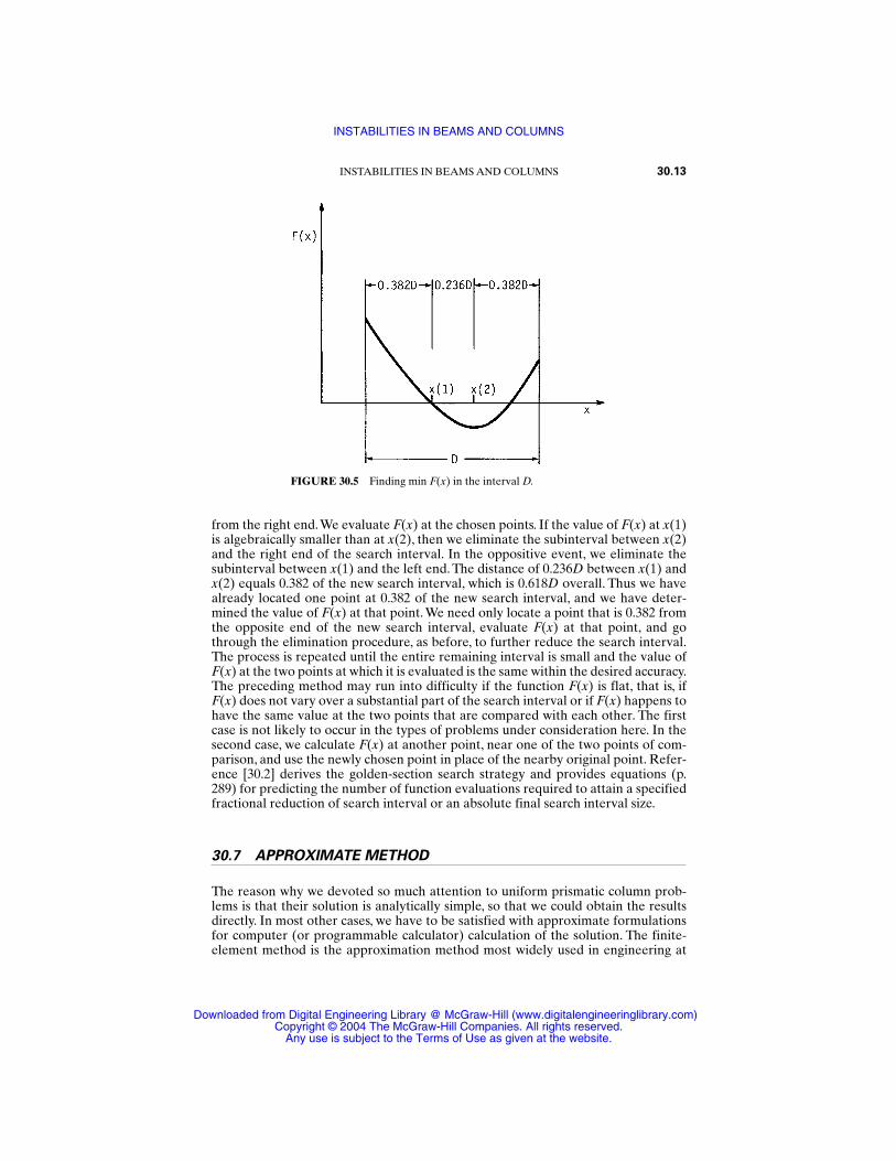
from the right end.We evaluate F(x) at the chosen points. If the value of F(x) at x(1)is algebraically smaller than at x(2), then we eliminate the subinterval between x(2)and the right end of the search interval. In the oppositive event, we eliminate thesubinterval between x(1) and the left end. The distance of 0.236D between x(1) andx(2) equals 0.382 of the new search interval, which is 0.618D overall. Thus we havealready located one point at 0.382 of the new search interval, and we have deter-mined the value of F(x) at that point. We need only locate a point that is 0.382 fromthe opposite end of the new search interval, evaluate F(x) at that point, and gothrough the elimination procedure, as before, to further reduce the search interval.The process is repeated until the entire remaining interval is small and the value ofF(x) at the two points at which it is evaluated is the same within the desired accuracy.The preceding method may run into difficulty if the function F(x) is flat, that is, ifF(x) does not vary over a substantial part of the search interval or if F(x) happens tohave the same value at the two points that are compared with each other. The firstcase is not likely to occur in the types of problems under consideration here. In thesecond case, we calculate F(x) at another point, near one of the two points of com-parison, and use the newly chosen point in place of the nearby original point. Refer-ence [30.2] derives the golden-section search strategy and provides equations (p.289) for predicting the number of function evaluations required to attain a specifiedfractional reduction of search interval or an absolute final search interval size.
30.7 APPROXIMATE METHOD
The reason why we devoted so much attention to uniform prismatic column prob-lems is that their solution is analytically simple, so that we could obtain the resultsdirectly. In most other cases, we have to be satisfied with approximate formulationsfor computer (or programmable calculator) calculation of the solution. The finite-element method is the approximation method most widely used in engineering at
INSTABILITIES IN BEAMS AND COLUMNS 30.13
FIGURE 30.5 Finding min F(x) in the interval D.
INSTABILITIES IN BEAMS AND COLUMNS
Downloaded from Digital Engineering Library @ McGraw-Hill (www.digitalengineeringlibrary.com)Copyright © 2004 The McGraw-Hill Companies. All rights reserved.
Any use is subject to the Terms of Use as given at the website.
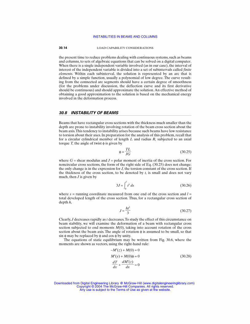
the present time to reduce problems dealing with continuous systems, such as beamsand columns, to sets of algebraic equations that can be solved on a digital computer.When there is a single independent variable involved (as in our case), the interval ofinterest of the independent variable is divided into a set of subintervals called finiteelements. Within each subinterval, the solution is represented by an arc that isdefined by a simple function, usually a polynomial of low degree. The curve result-ing from the connected arc segments should have a certain degree of smoothness(for the problems under discussion, the deflection curve and its first derivativeshould be continuous) and should approximate the solution.An effective method ofobtaining a good approximation to the solution is based on the mechanical energyinvolved in the deformation process.
30.8 INSTABILITY OF BEAMS
Beams that have rectangular cross sections with the thickness much smaller than thedepth are prone to instability involving rotation of the beam cross section about thebeam axis.This tendency to instability arises because such beams have low resistanceto torsion about their axes. In preparation for the analysis of this problem, recall thatfor a circular cylindrical member of length L and radius R, subjected to an axialtorque T, the angle of twist φ is given by
φ = (30.25)
where G = shear modulus and J = polar moment of inertia of the cross section. Fornoncircular cross sections, the form of the right side of Eq. (30.25) does not change;the only change is in the expression for J, the torsion constant of the cross section. Ifthe thickness of the cross section, to be denoted by t, is small and does not varymuch, then J is given by
3J = l
0t3 ds (30.26)
where s = running coordinate measured from one end of the cross section and l =total developed length of the cross section. Thus, for a rectangular cross section ofdepth h,
J = (30.27)
Clearly, J decreases rapidly as t decreases.To study the effect of this circumstance onbeam stability, we will examine the deformation of a beam with rectangular crosssection subjected to end moments M(0), taking into account rotation of the crosssection about the beam axis. The angle of rotation φ is assumed to be small, so thatsin φ may be replaced by φ and cos φ by unity.
The equations of static equilibrium may be written from Fig. 30.6, where themoments are shown as vectors, using the right-hand rule:
−M′(z) + M(0) = 0
M′(y) + M(0)φ = 0 (30.28)
+ = 0dM′(z)
dxdTdx
ht3
3
TLJG
30.14 LOAD CAPABILITY CONSIDERATIONS
INSTABILITIES IN BEAMS AND COLUMNS
Downloaded from Digital Engineering Library @ McGraw-Hill (www.digitalengineeringlibrary.com)Copyright © 2004 The McGraw-Hill Companies. All rights reserved.
Any use is subject to the Terms of Use as given at the website.
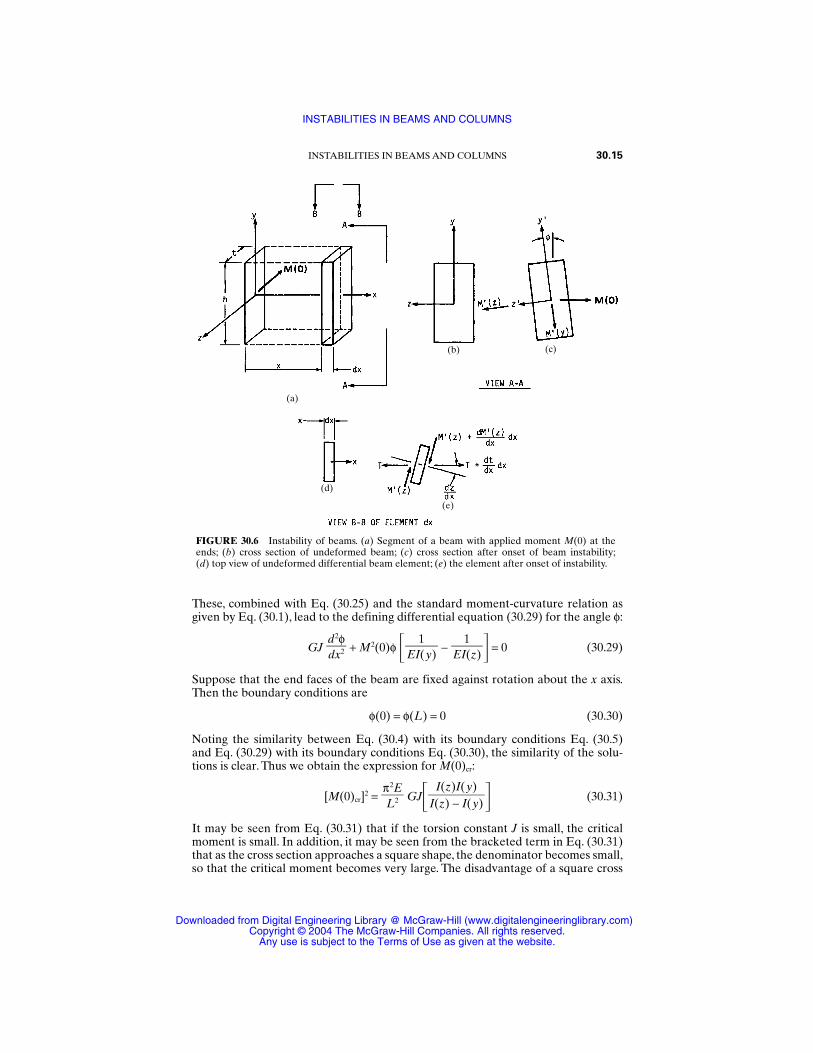
These, combined with Eq. (30.25) and the standard moment-curvature relation asgiven by Eq. (30.1), lead to the defining differential equation (30.29) for the angle φ:
GJ + M2(0)φ − = 0 (30.29)
Suppose that the end faces of the beam are fixed against rotation about the x axis.Then the boundary conditions are
φ(0) = φ(L) = 0 (30.30)
Noting the similarity between Eq. (30.4) with its boundary conditions Eq. (30.5)and Eq. (30.29) with its boundary conditions Eq. (30.30), the similarity of the solu-tions is clear. Thus we obtain the expression for M(0)cr:
[M(0)cr]2 = GJ (30.31)
It may be seen from Eq. (30.31) that if the torsion constant J is small, the criticalmoment is small. In addition, it may be seen from the bracketed term in Eq. (30.31)that as the cross section approaches a square shape, the denominator becomes small,so that the critical moment becomes very large. The disadvantage of a square cross
I(z)I(y)I(z) − I(y)
π2EL2
1EI(z)
1EI(y)
d2φdx2
INSTABILITIES IN BEAMS AND COLUMNS 30.15
FIGURE 30.6 Instability of beams. (a) Segment of a beam with applied moment M(0) at theends; (b) cross section of undeformed beam; (c) cross section after onset of beam instability;(d) top view of undeformed differential beam element; (e) the element after onset of instability.
(a)
(b) (c)
(e)
(d)
INSTABILITIES IN BEAMS AND COLUMNS
Downloaded from Digital Engineering Library @ McGraw-Hill (www.digitalengineeringlibrary.com)Copyright © 2004 The McGraw-Hill Companies. All rights reserved.
Any use is subject to the Terms of Use as given at the website.
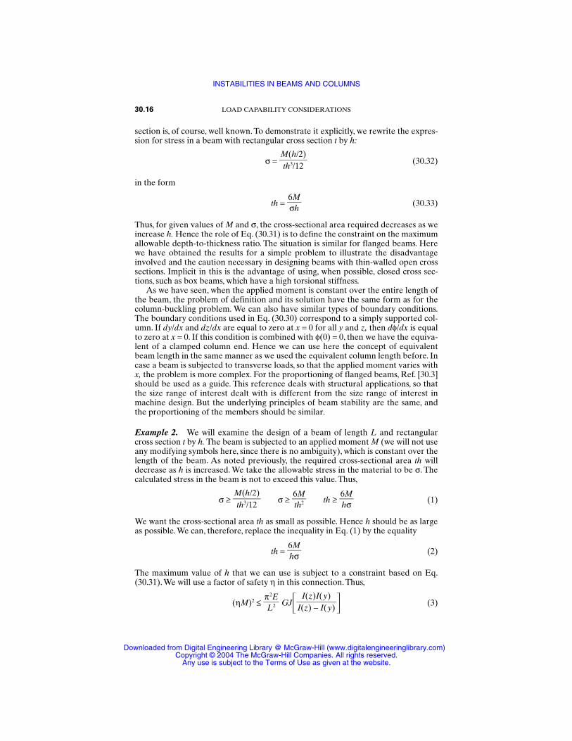
section is, of course, well known. To demonstrate it explicitly, we rewrite the expres-sion for stress in a beam with rectangular cross section t by h:
σ = (30.32)
in the form
th = (30.33)
Thus, for given values of M and σ, the cross-sectional area required decreases as weincrease h. Hence the role of Eq. (30.31) is to define the constraint on the maximumallowable depth-to-thickness ratio. The situation is similar for flanged beams. Herewe have obtained the results for a simple problem to illustrate the disadvantageinvolved and the caution necessary in designing beams with thin-walled open crosssections. Implicit in this is the advantage of using, when possible, closed cross sec-tions, such as box beams, which have a high torsional stiffness.
As we have seen, when the applied moment is constant over the entire length ofthe beam, the problem of definition and its solution have the same form as for thecolumn-buckling problem. We can also have similar types of boundary conditions.The boundary conditions used in Eq. (30.30) correspond to a simply supported col-umn. If dy/dx and dz/dx are equal to zero at x = 0 for all y and z, then dφ/dx is equalto zero at x = 0. If this condition is combined with φ(0) = 0, then we have the equiva-lent of a clamped column end. Hence we can use here the concept of equivalentbeam length in the same manner as we used the equivalent column length before. Incase a beam is subjected to transverse loads, so that the applied moment varies withx, the problem is more complex. For the proportioning of flanged beams, Ref. [30.3]should be used as a guide. This reference deals with structural applications, so thatthe size range of interest dealt with is different from the size range of interest inmachine design. But the underlying principles of beam stability are the same, andthe proportioning of the members should be similar.
Example 2. We will examine the design of a beam of length L and rectangularcross section t by h. The beam is subjected to an applied moment M (we will not useany modifying symbols here, since there is no ambiguity), which is constant over thelength of the beam. As noted previously, the required cross-sectional area th willdecrease as h is increased. We take the allowable stress in the material to be σ. Thecalculated stress in the beam is not to exceed this value. Thus,
σ ≥ σ ≥ th ≥ (1)
We want the cross-sectional area th as small as possible. Hence h should be as largeas possible. We can, therefore, replace the inequality in Eq. (1) by the equality
th = (2)
The maximum value of h that we can use is subject to a constraint based on Eq.(30.31). We will use a factor of safety η in this connection. Thus,
(ηM)2 ≤ GJ (3)I(z)I(y)
I(z) − I(y)
π2EL2
6Mhσ
6Mhσ
6Mth2
M(h/2)th3/12
6Mσh
M(h/2)th3/12
30.16 LOAD CAPABILITY CONSIDERATIONS
INSTABILITIES IN BEAMS AND COLUMNS
Downloaded from Digital Engineering Library @ McGraw-Hill (www.digitalengineeringlibrary.com)Copyright © 2004 The McGraw-Hill Companies. All rights reserved.
Any use is subject to the Terms of Use as given at the website.
Here
I(z) = I(y) = J = (4)
Using Eq. (4), we may write Eq. (3) as
(ηM)2 ≤ ht
2
(th)4 (5)
or, from Eq. (2),
(ηM)2 ≤ h6M
3σ
2
4
(6)
Since we seek to minimize th and maximize h, it may be seen from Eqs. (5) and (6)that the inequality sign may be replaced by the equality sign in those two equations.In Eq. (6), h is the only unspecified quantity. Further, since the square of t/h may beexpected to be small compared to unity, we can obtain substantially simpler approx-imations of reasonable accuracy. As a first step, we have
= 1 + ht
2
+ ht
4
+ ⋅⋅⋅ (7)
If we retain only the first two terms in the right side of Eq. (7), we have
ηM = 1 + h6M
3σ
2
h6M
3σ
6hMσ
2
(8)
If we also neglect the square of t/h in comparison with unity, we obtain
h = 1/5
(9)
as a reasonable first approximation. Thus if we take the factor of safety η as 1.5, wehave, for a steel member with E = 30 Mpsi, G = 12 Mpsi, and σ = 30 kpsi,
h = 1/5
= 8.62 1/5
(10)
This is a reasonable approximation to the optimal height of the beam cross section.It may also be used as a starting point for an iterative solution to the exact expres-sion, Eq. (6). For the purpose of iteration, we rewrite Eq. (6) as
h = 1/2
1/5
(11)
The value of h obtained from Eq. (9) is substituted into the right side of Eq. (11).Theresultant value of h thus obtained is then resubstituted into the right side of Eq. (11);the iterative process is continued until the computed value of h coincides with thevalue substituted into the right side to the desired degree of accuracy. Having deter-mined h, we can determine t from Eq. (2).
EG1 − [(6M)/(h3σ)]2
π(6M)2
ηLσ3
M2
L
M2
L
π(36)[(30 × 106)(12 × 106)]1/2
(1.5)(30 000)
π(6M)2(EG)1/2
ηLσ3
π(EG)1/2
6L
11 − (t/h)2
6Mhσ
11 − [(6M/(h3σ)]2
π2EG(6L)2
11 − (t/h)2
π2EG(6L)2
ht3
3
ht3
12
th3
12
INSTABILITIES IN BEAMS AND COLUMNS 30.17
INSTABILITIES IN BEAMS AND COLUMNS
Downloaded from Digital Engineering Library @ McGraw-Hill (www.digitalengineeringlibrary.com)Copyright © 2004 The McGraw-Hill Companies. All rights reserved.
Any use is subject to the Terms of Use as given at the website.

REFERENCES
30.1 H. Herman, “On the Analysis of Uniform Prismatic Columns,” Transactions of theASME, Journal of Mechanical Design, vol. 103, 1981, pp. 274–276.
30.2 C. R. Mischke, Mathematical Model Building, 2d rev. ed., Iowa State University Press,Ames, 1980.
30.3 American Institute of Steel Construction, LRFD Manual of Steel Construction, 3d ed.,AISC, Chicago, 2003.
30.18 LOAD CAPABILITY CONSIDERATIONS
INSTABILITIES IN BEAMS AND COLUMNS
Downloaded from Digital Engineering Library @ McGraw-Hill (www.digitalengineeringlibrary.com)Copyright © 2004 The McGraw-Hill Companies. All rights reserved.
Any use is subject to the Terms of Use as given at the website.

CHAPTER 31VIBRATION AND CONTROL
OF VIBRATION
T. S. Sankar, Ph.D., Eng.Professor and Chairman
Department of Mechanical EngineeringConcordia University
Montreal, Quebec, Canada
R. B. Bhat, Ph.D.Associate Professor
Department of Mechanical EngineeringConcordia University
Montreal, Quebec, Canada
31.1 INTRODUCTION / 31.1
31.2 SINGLE-DEGREE-OF-FREEDOM SYSTEMS / 31.1
31.3 SYSTEMS WITH SEVERAL DEGREES OF FREEDOM / 31.19
31.4 VIBRATION ISOLATION / 31.28
REFERENCES / 31.30
31.1 INTRODUCTION
Vibration analysis and control of vibrations are important and integral aspects ofevery machine design procedure. Establishing an appropriate mathematical model,its analysis, interpretation of the solutions, and incorporation of these results in thedesign, testing, evaluation, maintenance, and troubleshooting require a sound under-standing of the principles of vibration. All the essential materials dealing with vari-ous aspects of machine vibrations are presented here in a form suitable for mostdesign applications. Readers are encouraged to consult the references for moredetails.
31.2 SINGLE-DEGREE-OF-FREEDOM SYSTEMS
31.2.1 Free Vibration
A single-degree-of-freedom system is shown in Fig. 31.1. It consists of a mass m con-strained by a spring of stiffness k, and a damper with viscous damping coefficient c.The stiffness coefficient k is defined as the spring force per unit deflection.The coef-
31.1
Source: STANDARD HANDBOOK OF MACHINE DESIGN
Downloaded from Digital Engineering Library @ McGraw-Hill (www.digitalengineeringlibrary.com)Copyright © 2004 The McGraw-Hill Companies. All rights reserved.
Any use is subject to the Terms of Use as given at the website.
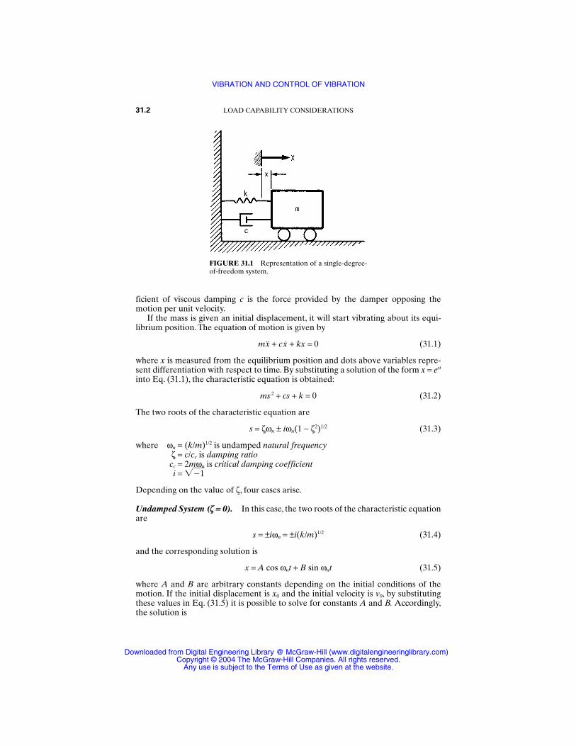
ficient of viscous damping c is the force provided by the damper opposing themotion per unit velocity.
If the mass is given an initial displacement, it will start vibrating about its equi-librium position. The equation of motion is given by
mx + cx + kx = 0 (31.1)
where x is measured from the equilibrium position and dots above variables repre-sent differentiation with respect to time. By substituting a solution of the form x = est
into Eq. (31.1), the characteristic equation is obtained:
ms 2 + cs + k = 0 (31.2)
The two roots of the characteristic equation are
s = ζωn ± iωn(1 − ζ2)1/2 (31.3)
where ωn = (k/m)1/2 is undamped natural frequencyζ = c/cc is damping ratiocc = 2mωn is critical damping coefficienti = 1
Depending on the value of ζ, four cases arise.
Undamped System (z = 0). In this case, the two roots of the characteristic equationare
s = ±iωn = ±i(k/m)1/2 (31.4)
and the corresponding solution is
x = A cos ωnt + B sin ωnt (31.5)
where A and B are arbitrary constants depending on the initial conditions of themotion. If the initial displacement is x0 and the initial velocity is v0, by substitutingthese values in Eq. (31.5) it is possible to solve for constants A and B. Accordingly,the solution is
31.2 LOAD CAPABILITY CONSIDERATIONS
FIGURE 31.1 Representation of a single-degree-of-freedom system.
VIBRATION AND CONTROL OF VIBRATION
Downloaded from Digital Engineering Library @ McGraw-Hill (www.digitalengineeringlibrary.com)Copyright © 2004 The McGraw-Hill Companies. All rights reserved.
Any use is subject to the Terms of Use as given at the website.
x = x0 cos ωnt + sin ωnt (31.6)
Here, ωn is the natural frequency of the system in radians per second (rad/s), whichis the frequency at which the system executes free vibrations. The natural frequencyis
fn = (31.7)
where fn is in cycles per second, or hertz (Hz). The period for one oscillation is
τ = = (31.8)
The solution given in Eq. (31.6) can also be expressed in the form
x = X cos (ωn − θ) (31.9)
where
X = x 02 +
2
1/2
θ = tan−1 (31.10)
The motion is harmonic with a phase angle θ as given in Eq. (31.9) and is showngraphically in Fig. 31.4.
Underdamped System (0 < z < 1). When the system damping is less than the criti-cal damping, the solution is
x = [exp(−ζωnt)] (A cos ωdt + B sin ωdt) (31.11)
where
ωd = ωn(1 − ζ2)1/2 (31.12)
is the damped natural frequency and A and B are arbitrary constants to be deter-mined from the initial conditions. For an initial amplitude of x0 and initial velocity v0,
x = [exp (−ζωnt)] x0 cos ωdt + sin ωdt (31.13)
which can be written in the form
x = [exp (−ζωnt)] X cos (ωdt − θ)
X = x 02 +
2
1/2
(31.14)
and
θ = tan−1
An underdamped system will execute exponentially decaying oscillations, as showngraphically in Fig. 31.2.
ζωnx0 + v0
ωd
ζωnx0 + v0
ωd
ζωnx0 + v0
ωd
v0ωnx0
v0ωn
2πωn
1fn
ωn2π
v0ωn
VIBRATION AND CONTROL OF VIBRATION 31.3
VIBRATION AND CONTROL OF VIBRATION
Downloaded from Digital Engineering Library @ McGraw-Hill (www.digitalengineeringlibrary.com)Copyright © 2004 The McGraw-Hill Companies. All rights reserved.
Any use is subject to the Terms of Use as given at the website.
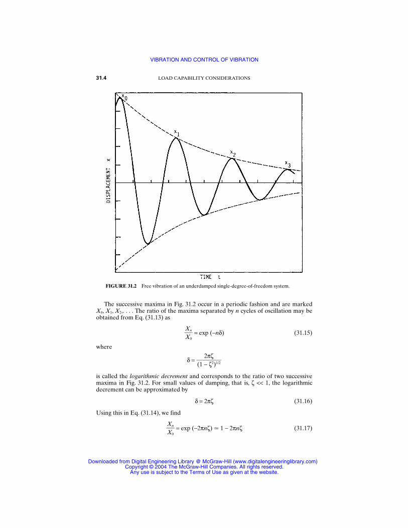
The successive maxima in Fig. 31.2 occur in a periodic fashion and are marked X0, X1, X2,. . . . The ratio of the maxima separated by n cycles of oscillation may beobtained from Eq. (31.13) as
= exp (−nδ) (31.15)
where
δ =
is called the logarithmic decrement and corresponds to the ratio of two successivemaxima in Fig. 31.2. For small values of damping, that is, ζ << 1, the logarithmicdecrement can be approximated by
δ = 2πζ (31.16)
Using this in Eq. (31.14), we find
= exp (−2πnζ) 1 − 2πnζ (31.17)XnX0
2πζ(1 − ζ2)1/2
XnX0
31.4 LOAD CAPABILITY CONSIDERATIONS
FIGURE 31.2 Free vibration of an underdamped single-degree-of-freedom system.
VIBRATION AND CONTROL OF VIBRATION
Downloaded from Digital Engineering Library @ McGraw-Hill (www.digitalengineeringlibrary.com)Copyright © 2004 The McGraw-Hill Companies. All rights reserved.
Any use is subject to the Terms of Use as given at the website.
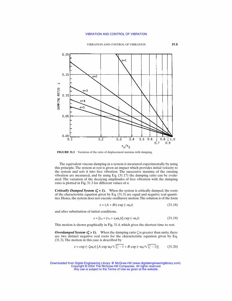
VIBRATION AND CONTROL OF VIBRATION 31.5
FIGURE 31.3 Variation of the ratio of displacement maxima with damping.
The equivalent viscous damping in a system is measured experimentally by usingthis principle. The system at rest is given an impact which provides initial velocity tothe system and sets it into free vibration. The successive maxima of the ensuingvibration are measured, and by using Eq. (31.17) the damping ratio can be evalu-ated. The variation of the decaying amplitudes of free vibration with the dampingratio is plotted in Fig. 31.3 for different values of n.
Critically Damped System (z = 1). When the system is critically damped, the rootsof the characteristic equation given by Eq. (31.3) are equal and negative real quanti-ties. Hence, the system does not execute oscillatory motion.The solution is of the form
x = (A + Bt) exp (−ωnt) (31.18)
and after substitution of initial conditions,
x = [x0 + (v0 + x0ωn)t] exp (−ωnt) (31.19)
This motion is shown graphically in Fig. 31.4, which gives the shortest time to rest.
Overdamped System (z > 1). When the damping ratio ζ is greater than unity, thereare two distinct negative real roots for the characteristic equation given by Eq.(31.3). The motion in this case is described by
x = exp (−ζωnt) [A exp ωntζ2 − 1 + B exp (−ωntζ2 − 1)] (31.20)
VIBRATION AND CONTROL OF VIBRATION
Downloaded from Digital Engineering Library @ McGraw-Hill (www.digitalengineeringlibrary.com)Copyright © 2004 The McGraw-Hill Companies. All rights reserved.
Any use is subject to the Terms of Use as given at the website.
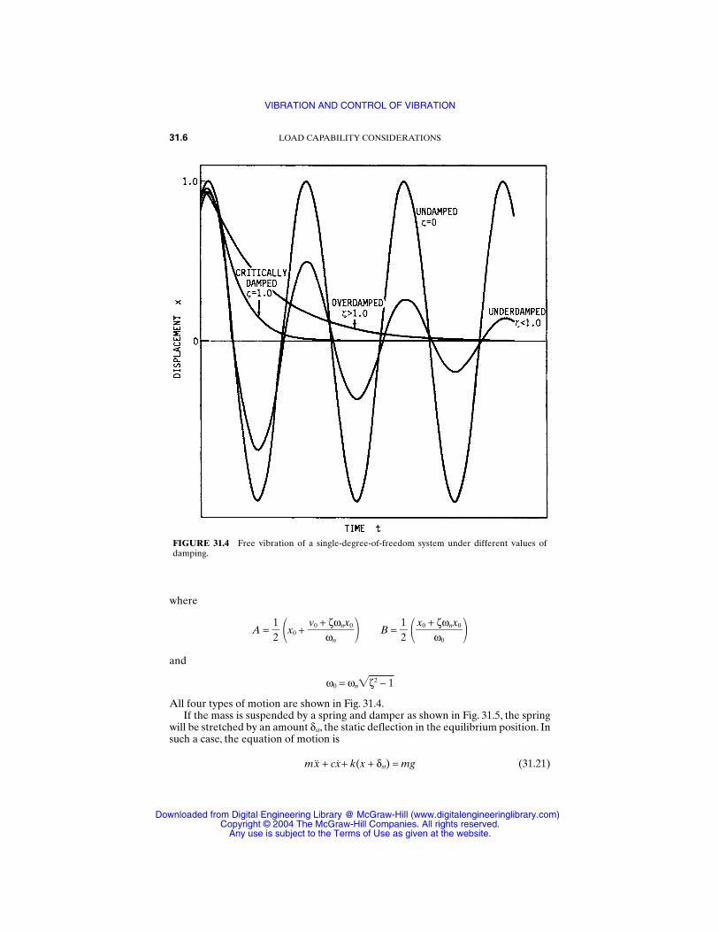
where
A = x0 + B = and
ω0 = ωnζ2 − 1
All four types of motion are shown in Fig. 31.4.If the mass is suspended by a spring and damper as shown in Fig. 31.5, the spring
will be stretched by an amount δst, the static deflection in the equilibrium position. Insuch a case, the equation of motion is
mx + cx+ k(x + δst) = mg (31.21)
x0 + ζωnx0
ω0
12
v0 + ζωnx0
ωn
12
31.6 LOAD CAPABILITY CONSIDERATIONS
FIGURE 31.4 Free vibration of a single-degree-of-freedom system under different values ofdamping.
VIBRATION AND CONTROL OF VIBRATION
Downloaded from Digital Engineering Library @ McGraw-Hill (www.digitalengineeringlibrary.com)Copyright © 2004 The McGraw-Hill Companies. All rights reserved.
Any use is subject to the Terms of Use as given at the website.
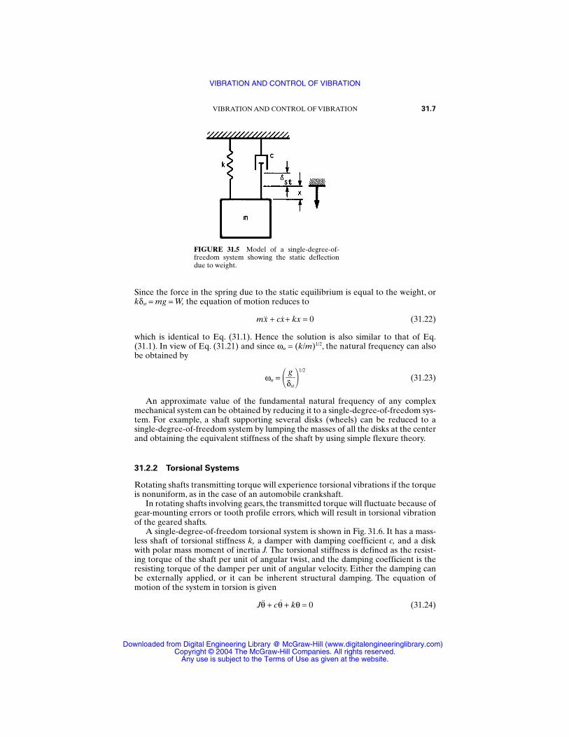
Since the force in the spring due to the static equilibrium is equal to the weight, orkδst = mg = W, the equation of motion reduces to
mx + cx+ kx = 0 (31.22)
which is identical to Eq. (31.1). Hence the solution is also similar to that of Eq.(31.1). In view of Eq. (31.21) and since ωn = (k/m)1/2, the natural frequency can alsobe obtained by
ωn = 1/2
(31.23)
An approximate value of the fundamental natural frequency of any complexmechanical system can be obtained by reducing it to a single-degree-of-freedom sys-tem. For example, a shaft supporting several disks (wheels) can be reduced to a single-degree-of-freedom system by lumping the masses of all the disks at the centerand obtaining the equivalent stiffness of the shaft by using simple flexure theory.
31.2.2 Torsional Systems
Rotating shafts transmitting torque will experience torsional vibrations if the torqueis nonuniform, as in the case of an automobile crankshaft.
In rotating shafts involving gears, the transmitted torque will fluctuate because ofgear-mounting errors or tooth profile errors, which will result in torsional vibrationof the geared shafts.
A single-degree-of-freedom torsional system is shown in Fig. 31.6. It has a mass-less shaft of torsional stiffness k, a damper with damping coefficient c, and a diskwith polar mass moment of inertia J. The torsional stiffness is defined as the resist-ing torque of the shaft per unit of angular twist, and the damping coefficient is theresisting torque of the damper per unit of angular velocity. Either the damping canbe externally applied, or it can be inherent structural damping. The equation ofmotion of the system in torsion is given
Jθ + cθ + kθ = 0 (31.24)
gδst
VIBRATION AND CONTROL OF VIBRATION 31.7
FIGURE 31.5 Model of a single-degree-of-freedom system showing the static deflectiondue to weight.
VIBRATION AND CONTROL OF VIBRATION
Downloaded from Digital Engineering Library @ McGraw-Hill (www.digitalengineeringlibrary.com)Copyright © 2004 The McGraw-Hill Companies. All rights reserved.
Any use is subject to the Terms of Use as given at the website.
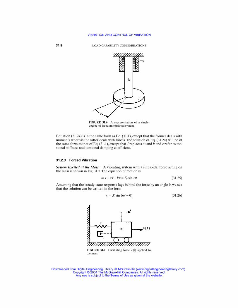
Equation (31.24) is in the same form as Eq. (31.1), except that the former deals withmoments whereas the latter deals with forces. The solution of Eq. (31.24) will be ofthe same form as that of Eq. (31.1), except that J replaces m and k and c refer to tor-sional stiffness and torsional damping coefficient.
31.2.3 Forced Vibration
System Excited at the Mass. A vibrating system with a sinusoidal force acting onthe mass is shown in Fig. 31.7. The equation of motion is
mx + cx + kx = F0 sin ωt (31.25)
Assuming that the steady-state response lags behind the force by an angle θ, we seethat the solution can be written in the form
xs = X sin (ωt − θ) (31.26)
31.8 LOAD CAPABILITY CONSIDERATIONS
FIGURE 31.6 A representation of a single-degree-of-freedom torsional system.
FIGURE 31.7 Oscillating force F(t) applied tothe mass.
VIBRATION AND CONTROL OF VIBRATION
Downloaded from Digital Engineering Library @ McGraw-Hill (www.digitalengineeringlibrary.com)Copyright © 2004 The McGraw-Hill Companies. All rights reserved.
Any use is subject to the Terms of Use as given at the website.
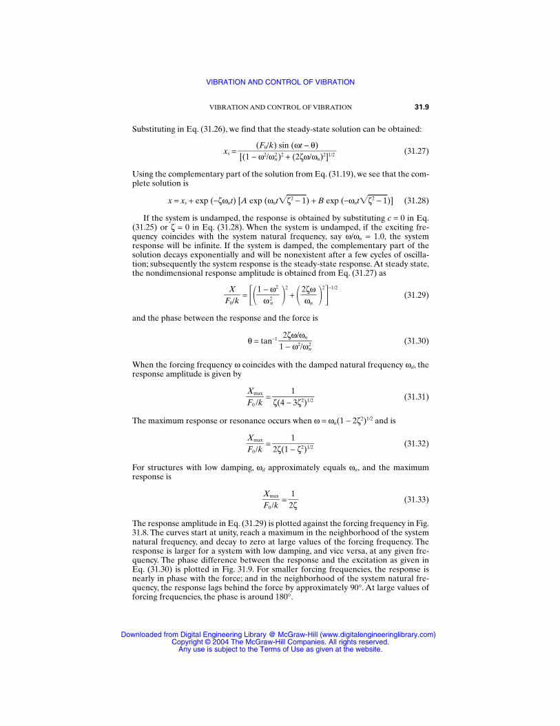
Substituting in Eq. (31.26), we find that the steady-state solution can be obtained:
xs = (31.27)
Using the complementary part of the solution from Eq. (31.19), we see that the com-plete solution is
x = xs + exp (−ζωnt) [A exp (ωntζ2 − 1) + B exp (−ωntζ2 − 1)] (31.28)
If the system is undamped, the response is obtained by substituting c = 0 in Eq.(31.25) or ζ = 0 in Eq. (31.28). When the system is undamped, if the exciting fre-quency coincides with the system natural frequency, say ω/ωn = 1.0, the systemresponse will be infinite. If the system is damped, the complementary part of thesolution decays exponentially and will be nonexistent after a few cycles of oscilla-tion; subsequently the system response is the steady-state response. At steady state,the nondimensional response amplitude is obtained from Eq. (31.27) as
= 2
+ 2
−1/2
(31.29)
and the phase between the response and the force is
θ = tan−1 (31.30)
When the forcing frequency ω coincides with the damped natural frequency ωd, theresponse amplitude is given by
= (31.31)
The maximum response or resonance occurs when ω = ωn(1 − 2ζ2)1/2 and is
= (31.32)
For structures with low damping, ωd approximately equals ωn, and the maximumresponse is
= (31.33)
The response amplitude in Eq. (31.29) is plotted against the forcing frequency in Fig.31.8. The curves start at unity, reach a maximum in the neighborhood of the systemnatural frequency, and decay to zero at large values of the forcing frequency. Theresponse is larger for a system with low damping, and vice versa, at any given fre-quency. The phase difference between the response and the excitation as given inEq. (31.30) is plotted in Fig. 31.9. For smaller forcing frequencies, the response isnearly in phase with the force; and in the neighborhood of the system natural fre-quency, the response lags behind the force by approximately 90°. At large values offorcing frequencies, the phase is around 180°.
12ζ
XmaxF0 /k
12ζ(1 − ζ2)1/2
XmaxF0 /k
1ζ(4 − 3ζ2)1/2
XmaxF0 /k
2ζω/ωn1 − ω2/ωn
2
2ζωωn
1 − ω2
ω n
2
XF0/k
(F0/k) sin (ωt − θ)[(1 − ω2/ωn
2)2 + (2ζω/ωn)2]1/2
VIBRATION AND CONTROL OF VIBRATION 31.9
VIBRATION AND CONTROL OF VIBRATION
Downloaded from Digital Engineering Library @ McGraw-Hill (www.digitalengineeringlibrary.com)Copyright © 2004 The McGraw-Hill Companies. All rights reserved.
Any use is subject to the Terms of Use as given at the website.
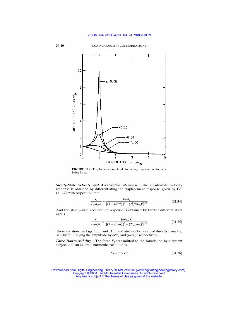
Steady-State Velocity and Acceleration Response. The steady-state velocityresponse is obtained by differentiating the displacement response, given by Eq.(31.27), with respect to time:
= (31.34)
And the steady-state acceleration response is obtained by further differentiationand is
= (31.35)
These are shown in Figs. 31.10 and 31.11 and also can be obtained directly from Fig.31.8 by multiplying the amplitude by ω/ωn and (ω/ωn)2, respectively.
Force Transmissibility. The force FT transmitted to the foundation by a systemsubjected to an external harmonic excitation is
FT = cx + kx (31.36)
(ω/ωn)2
[(1 − ω2/ω n
2 )2 + (2ζω/ωn)2]1/2
xsF0ωn
2 /k
ω/ωn[(1 − ω2/ωn
2 )2 + (2ζω/ωn)2]1/2
xsF0ωn/k
31.10 LOAD CAPABILITY CONSIDERATIONS
FIGURE 31.8 Displacement-amplitude frequency response due to oscil-lating force.
VIBRATION AND CONTROL OF VIBRATION
Downloaded from Digital Engineering Library @ McGraw-Hill (www.digitalengineeringlibrary.com)Copyright © 2004 The McGraw-Hill Companies. All rights reserved.
Any use is subject to the Terms of Use as given at the website.
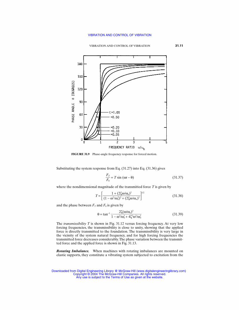
Substituting the system response from Eq. (31.27) into Eq. (31.36) gives
= T sin (ωt − θ) (31.37)
where the nondimensional magnitude of the transmitted force T is given by
T = 1/2
(31.38)
and the phase between FT and F0 is given by
θ = tan−1 (31.39)
The transmissibility T is shown in Fig. 31.12 versus forcing frequency. At very lowforcing frequencies, the transmissibility is close to unity, showing that the appliedforce is directly transmitted to the foundation. The transmissibility is very large inthe vicinity of the system natural frequency, and for high forcing frequencies thetransmitted force decreases considerably.The phase variation between the transmit-ted force and the applied force is shown in Fig. 31.13.
Rotating Imbalance. When machines with rotating imbalances are mounted onelastic supports, they constitute a vibrating system subjected to excitation from the
2ζ(ω/ωn)3
1 − ω2/ωn
2 + 4ζ2ω2/ωn2
1 + (2ζω/ωn)2
(1 − ω2/ωn
2)2 + (2ζω/ωn)2
FTF0
VIBRATION AND CONTROL OF VIBRATION 31.11
FIGURE 31.9 Phase-angle frequency response for forced motion.
VIBRATION AND CONTROL OF VIBRATION
Downloaded from Digital Engineering Library @ McGraw-Hill (www.digitalengineeringlibrary.com)Copyright © 2004 The McGraw-Hill Companies. All rights reserved.
Any use is subject to the Terms of Use as given at the website.
rotating imbalance. If the natural frequency of the system coincides with the fre-quency of rotation of the machine imbalance, it will result in severe vibrations of themachine and the support structure.
Consider a machine of mass M supported as shown in Fig. 31.14. Let the imbal-ance be a mass m with an eccentricity e and rotating with a frequency ω. Considerthe motion x of the mass M − m, with xm as the motion of the unbalanced mass m rel-ative to the machine mass M. The equation of motion is
(M − m)x + m( x + xm) + cx + kx = 0 (31.40)
The motion of the unbalanced mass relative to the machine is
xm = e sin ωt (31.41)
Substitution in Eq. (31.40) leads to
Mx + cx + kx = meω2 sin ωt (31.42)
31.12 LOAD CAPABILITY CONSIDERATIONS
FIGURE 31.10 Velocity frequency response.
VIBRATION AND CONTROL OF VIBRATION
Downloaded from Digital Engineering Library @ McGraw-Hill (www.digitalengineeringlibrary.com)Copyright © 2004 The McGraw-Hill Companies. All rights reserved.
Any use is subject to the Terms of Use as given at the website.
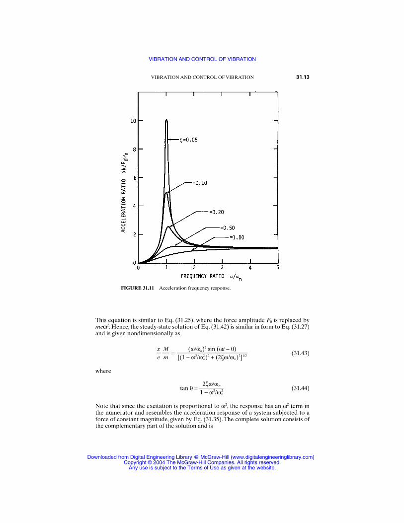
This equation is similar to Eq. (31.25), where the force amplitude F0 is replaced bymeω2. Hence, the steady-state solution of Eq. (31.42) is similar in form to Eq. (31.27)and is given nondimensionally as
= (31.43)
where
tan θ = (31.44)
Note that since the excitation is proportional to ω2, the response has an ω2 term inthe numerator and resembles the acceleration response of a system subjected to aforce of constant magnitude, given by Eq. (31.35). The complete solution consists ofthe complementary part of the solution and is
2ζω/ωn1 − ω2/ωn
2
(ω/ωn)2 sin (ωt − θ)[(1 − ω2/ωn
2)2 + (2ζω/ωn)2]1/2
Mm
xe
VIBRATION AND CONTROL OF VIBRATION 31.13
FIGURE 31.11 Acceleration frequency response.
VIBRATION AND CONTROL OF VIBRATION
Downloaded from Digital Engineering Library @ McGraw-Hill (www.digitalengineeringlibrary.com)Copyright © 2004 The McGraw-Hill Companies. All rights reserved.
Any use is subject to the Terms of Use as given at the website.
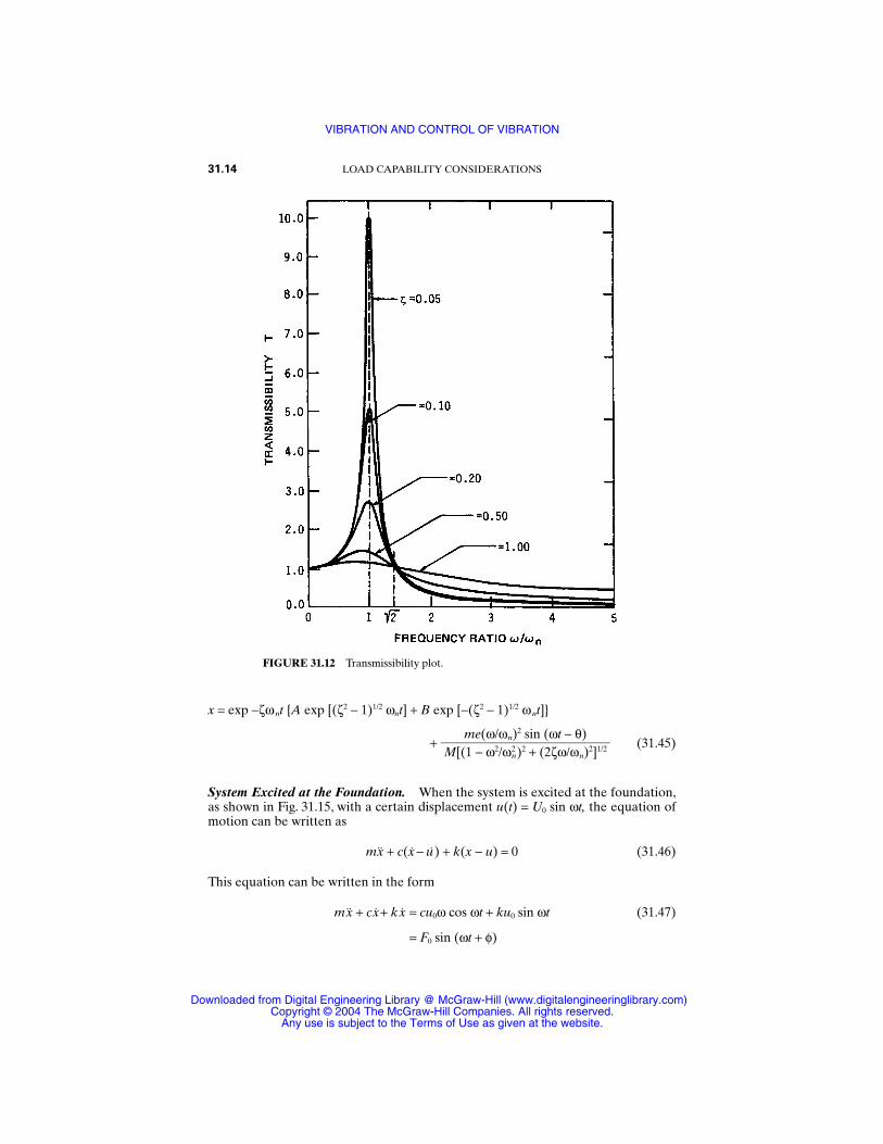
x = exp −ζωnt A exp [(ζ2 − 1)1/2 ωnt] + B exp [−(ζ2 − 1)1/2 ωnt]
+ (31.45)
System Excited at the Foundation. When the system is excited at the foundation,as shown in Fig. 31.15, with a certain displacement u(t) = U0 sin ωt, the equation ofmotion can be written as
mx + c(x − u) + k(x − u) = 0 (31.46)
This equation can be written in the form
mx + cx+ kx = cu0ω cos ωt + ku0 sin ωt (31.47)
= F0 sin (ωt + φ)
me(ω/ωn)2 sin (ωt − θ)M[(1 − ω2/ωn
2)2 + (2ζω/ωn)2]1/2
31.14 LOAD CAPABILITY CONSIDERATIONS
FIGURE 31.12 Transmissibility plot.
VIBRATION AND CONTROL OF VIBRATION
Downloaded from Digital Engineering Library @ McGraw-Hill (www.digitalengineeringlibrary.com)Copyright © 2004 The McGraw-Hill Companies. All rights reserved.
Any use is subject to the Terms of Use as given at the website.
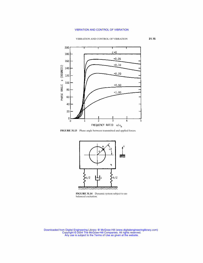
VIBRATION AND CONTROL OF VIBRATION 31.15
FIGURE 31.13 Phase angle between transmitted and applied forces.
FIGURE 31.14 Dynamic system subject to un-balanced excitation.
VIBRATION AND CONTROL OF VIBRATION
Downloaded from Digital Engineering Library @ McGraw-Hill (www.digitalengineeringlibrary.com)Copyright © 2004 The McGraw-Hill Companies. All rights reserved.
Any use is subject to the Terms of Use as given at the website.
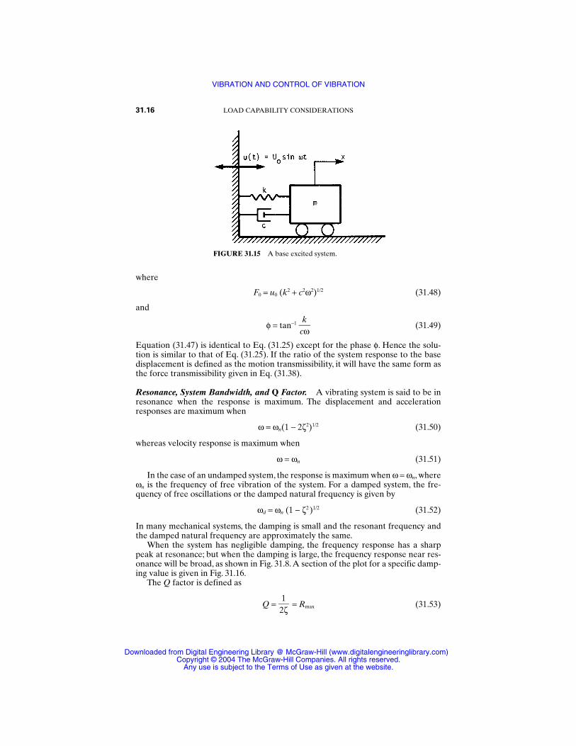
where
F0 = u0 (k2 + c2ω2)1/2 (31.48)
and
φ = tan−1 ckω (31.49)
Equation (31.47) is identical to Eq. (31.25) except for the phase φ. Hence the solu-tion is similar to that of Eq. (31.25). If the ratio of the system response to the basedisplacement is defined as the motion transmissibility, it will have the same form asthe force transmissibility given in Eq. (31.38).
Resonance, System Bandwidth, and Q Factor. A vibrating system is said to be inresonance when the response is maximum. The displacement and accelerationresponses are maximum when
ω = ωn(1 − 2ζ2)1/2 (31.50)
whereas velocity response is maximum when
ω = ωn (31.51)
In the case of an undamped system, the response is maximum when ω = ωn, whereωn is the frequency of free vibration of the system. For a damped system, the fre-quency of free oscillations or the damped natural frequency is given by
ωd = ωn (1 − ζ2)1/2 (31.52)
In many mechanical systems, the damping is small and the resonant frequency andthe damped natural frequency are approximately the same.
When the system has negligible damping, the frequency response has a sharppeak at resonance; but when the damping is large, the frequency response near res-onance will be broad, as shown in Fig. 31.8.A section of the plot for a specific damp-ing value is given in Fig. 31.16.
The Q factor is defined as
Q = = Rmax (31.53)1
2ζ
31.16 LOAD CAPABILITY CONSIDERATIONS
FIGURE 31.15 A base excited system.
VIBRATION AND CONTROL OF VIBRATION
Downloaded from Digital Engineering Library @ McGraw-Hill (www.digitalengineeringlibrary.com)Copyright © 2004 The McGraw-Hill Companies. All rights reserved.
Any use is subject to the Terms of Use as given at the website.
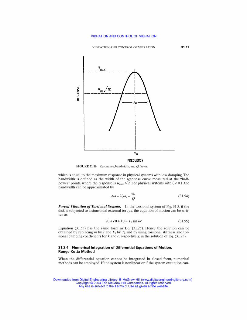
which is equal to the maximum response in physical systems with low damping. Thebandwidth is defined as the width of the response curve measured at the “half-power” points, where the response is Rmax/2. For physical systems with ζ < 0.1, thebandwidth can be approximated by
∆ω = 2ζωn = (31.54)
Forced Vibration of Torsional Systems. In the torsional system of Fig. 31.3, if thedisk is subjected to a sinusoidal external torque, the equation of motion can be writ-ten as
Jθ + cθ + kθ = T0 sin ωt (31.55)
Equation (31.55) has the same form as Eq. (31.25). Hence the solution can beobtained by replacing m by J and F0 by T0 and by using torsional stiffness and tor-sional damping coefficients for k and c, respectively, in the solution of Eq. (31.25).
31.2.4 Numerical Integration of Differential Equations of Motion: Runge-Kutta Method
When the differential equation cannot be integrated in closed form, numericalmethods can be employed. If the system is nonlinear or if the system excitation can-
ωnQ
VIBRATION AND CONTROL OF VIBRATION 31.17
FIGURE 31.16 Resonance, bandwidth, and Q factor.
VIBRATION AND CONTROL OF VIBRATION
Downloaded from Digital Engineering Library @ McGraw-Hill (www.digitalengineeringlibrary.com)Copyright © 2004 The McGraw-Hill Companies. All rights reserved.
Any use is subject to the Terms of Use as given at the website.
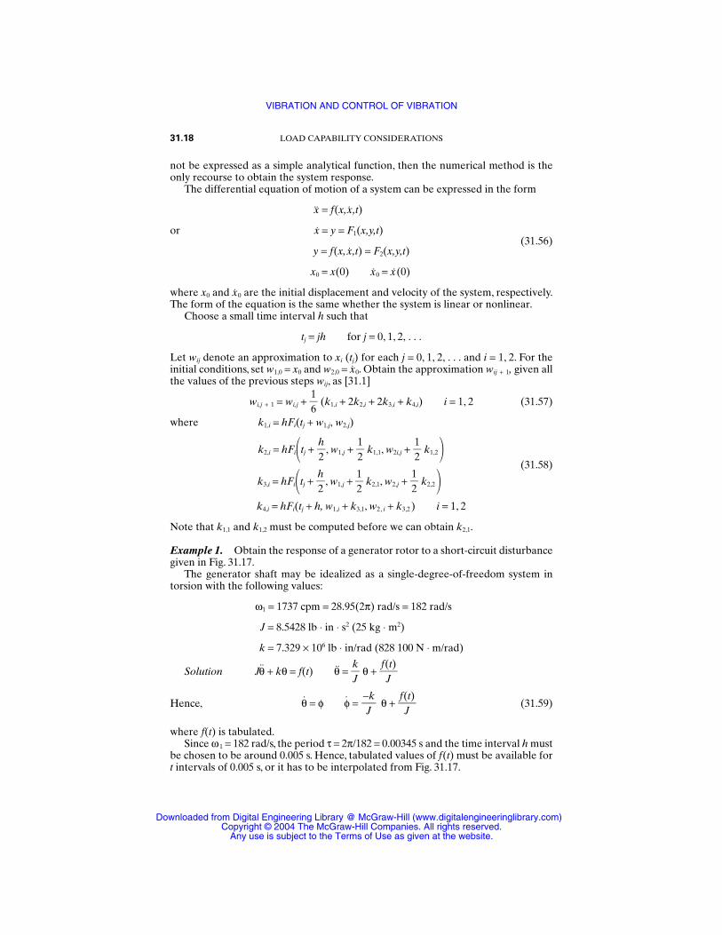
not be expressed as a simple analytical function, then the numerical method is theonly recourse to obtain the system response.
The differential equation of motion of a system can be expressed in the form
x = f(x,x,t)
or x = y = F1(x,y,t)(31.56)
y = f(x, x,t) = F2(x,y,t)
x0 = x(0) x0 = x(0)
where x0 and x0 are the initial displacement and velocity of the system, respectively.The form of the equation is the same whether the system is linear or nonlinear.
Choose a small time interval h such that
tj = jh for j = 0, 1, 2, . . .
Let wij denote an approximation to xi (tj) for each j = 0, 1, 2, . . . and i = 1, 2. For theinitial conditions, set w1,0 = x0 and w2,0 = x0. Obtain the approximation wij + 1, given allthe values of the previous steps wij, as [31.1]
wi,j + 1 = wi,j + (k1,i + 2k2,i + 2k3,i + k4,i) i = 1, 2 (31.57)
where k1,i = hFi(tj + w1,j, w2,j)
k2,i = hFitj + , w1,j + k1,1, w2i,j + k1,2k3,i = hFitj + , w1,j +
12
k2,1, w2,j + k2,2(31.58)
k4,i = hFi(tj + h, w1,i + k3,1, w2, i + k3,2 ) i = 1, 2
Note that k1,1 and k1,2 must be computed before we can obtain k2,1.
Example 1. Obtain the response of a generator rotor to a short-circuit disturbancegiven in Fig. 31.17.
The generator shaft may be idealized as a single-degree-of-freedom system intorsion with the following values:
ω1 = 1737 cpm = 28.95(2π) rad/s = 182 rad/s
J = 8.5428 lb ⋅ in ⋅ s2 (25 kg ⋅ m2)
k = 7.329 × 10⁶ lb ⋅ in/rad (828 100 N ⋅ m/rad)
Solution Jθ + kθ = f(t) θ = θ +
Hence, θ = φ φ = θ + (31.59)
where f(t) is tabulated.Since ω 1 = 182 rad/s, the period τ = 2π/182 = 0.00345 s and the time interval h must
be chosen to be around 0.005 s. Hence, tabulated values of f(t) must be available fort intervals of 0.005 s, or it has to be interpolated from Fig. 31.17.
f(t)
J−kJ
f(t)
JkJ
12
h2
12
12
h2
16
31.18 LOAD CAPABILITY CONSIDERATIONS
VIBRATION AND CONTROL OF VIBRATION
Downloaded from Digital Engineering Library @ McGraw-Hill (www.digitalengineeringlibrary.com)Copyright © 2004 The McGraw-Hill Companies. All rights reserved.
Any use is subject to the Terms of Use as given at the website.
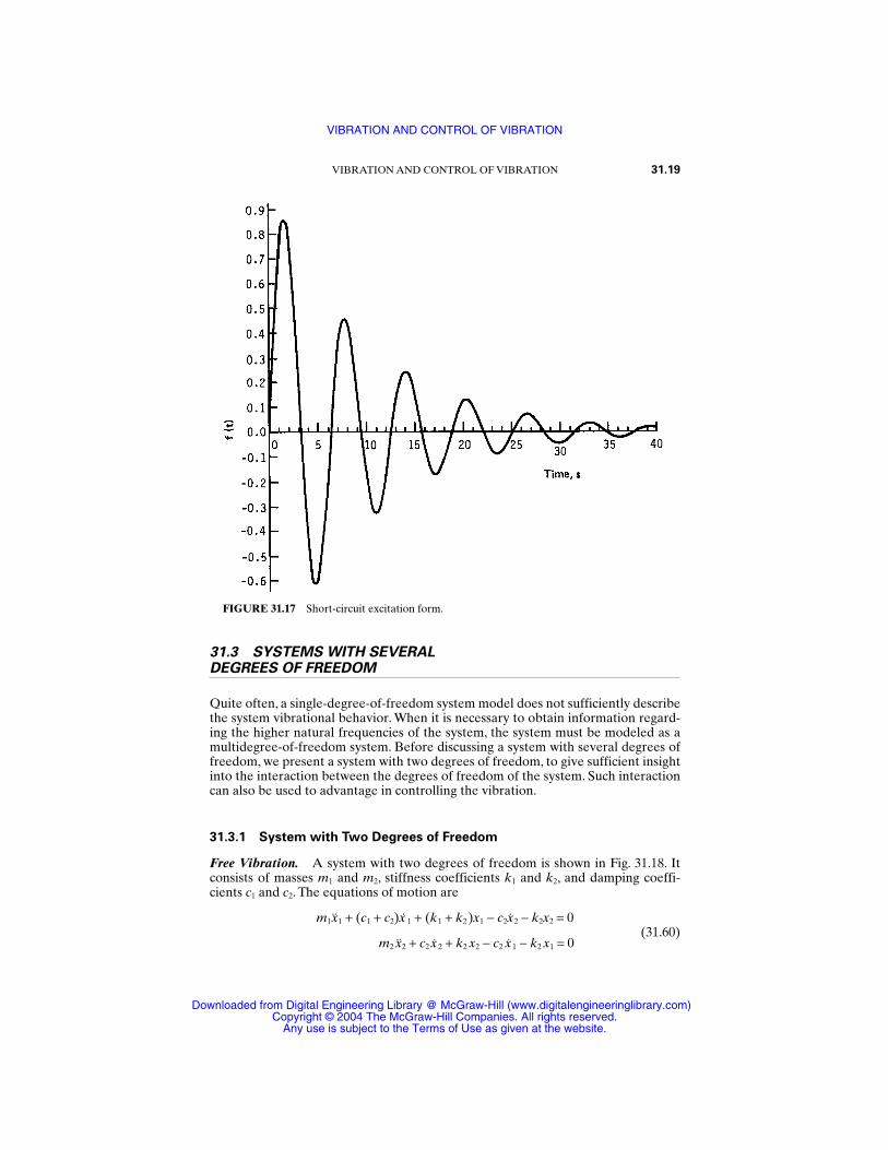
31.3 SYSTEMS WITH SEVERAL DEGREES OF FREEDOM
Quite often, a single-degree-of-freedom system model does not sufficiently describethe system vibrational behavior. When it is necessary to obtain information regard-ing the higher natural frequencies of the system, the system must be modeled as amultidegree-of-freedom system. Before discussing a system with several degrees offreedom, we present a system with two degrees of freedom, to give sufficient insightinto the interaction between the degrees of freedom of the system. Such interactioncan also be used to advantage in controlling the vibration.
31.3.1 System with Two Degrees of Freedom
Free Vibration. A system with two degrees of freedom is shown in Fig. 31.18. Itconsists of masses m1 and m2, stiffness coefficients k1 and k2, and damping coeffi-cients c1 and c2. The equations of motion are
m1x1 + (c1 + c2)x 1 + (k1 + k2)x1 − c2x2 − k2x2 = 0(31.60)
m2 x2 + c2 x2 + k2 x2 − c2 x1 − k2 x1 = 0
VIBRATION AND CONTROL OF VIBRATION 31.19
FIGURE 31.17 Short-circuit excitation form.
VIBRATION AND CONTROL OF VIBRATION
Downloaded from Digital Engineering Library @ McGraw-Hill (www.digitalengineeringlibrary.com)Copyright © 2004 The McGraw-Hill Companies. All rights reserved.
Any use is subject to the Terms of Use as given at the website.
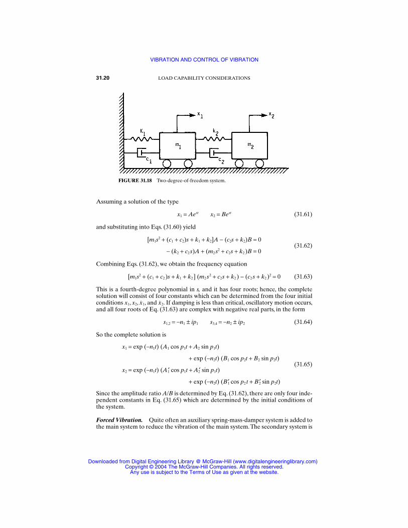
Assuming a solution of the type
x1 = Aest x2 = Best (31.61)
and substituting into Eqs. (31.60) yield
[m1s2 + (c1 + c2)s + k1 + k2]A − (c2s + k2)B = 0(31.62)
− (k2 + c2s)A + (m2 s2 + c2s + k2)B = 0
Combining Eqs. (31.62), we obtain the frequency equation
[m1s2 + (c1 + c2 )s + k1 + k2 ] (m2s2 + c2s + k2) − (c2s + k2 )2 = 0 (31.63)
This is a fourth-degree polynomial in s, and it has four roots; hence, the completesolution will consist of four constants which can be determined from the four initialconditions x1, x2, x1, and x2. If damping is less than critical, oscillatory motion occurs,and all four roots of Eq. (31.63) are complex with negative real parts, in the form
s1,2 = −n1 ± ip1 s3,4 = −n2 ± ip2 (31.64)
So the complete solution is
x1 = exp (−n1t) (A1 cos p1t + A2 sin p1t)
+ exp (−n2t) (B1 cos p2t + B2 sin p2t)(31.65)
x2 = exp (−n1t) (A1′ cos p1t + A2′ sin p1t)
+ exp (−n2t) (B1′ cos p2 t + B2′ sin p2t)
Since the amplitude ratio A/B is determined by Eq. (31.62), there are only four inde-pendent constants in Eq. (31.65) which are determined by the initial conditions ofthe system.
Forced Vibration. Quite often an auxiliary spring-mass-damper system is added tothe main system to reduce the vibration of the main system.The secondary system is
31.20 LOAD CAPABILITY CONSIDERATIONS
FIGURE 31.18 Two-degree-of-freedom system.
VIBRATION AND CONTROL OF VIBRATION
Downloaded from Digital Engineering Library @ McGraw-Hill (www.digitalengineeringlibrary.com)Copyright © 2004 The McGraw-Hill Companies. All rights reserved.
Any use is subject to the Terms of Use as given at the website.
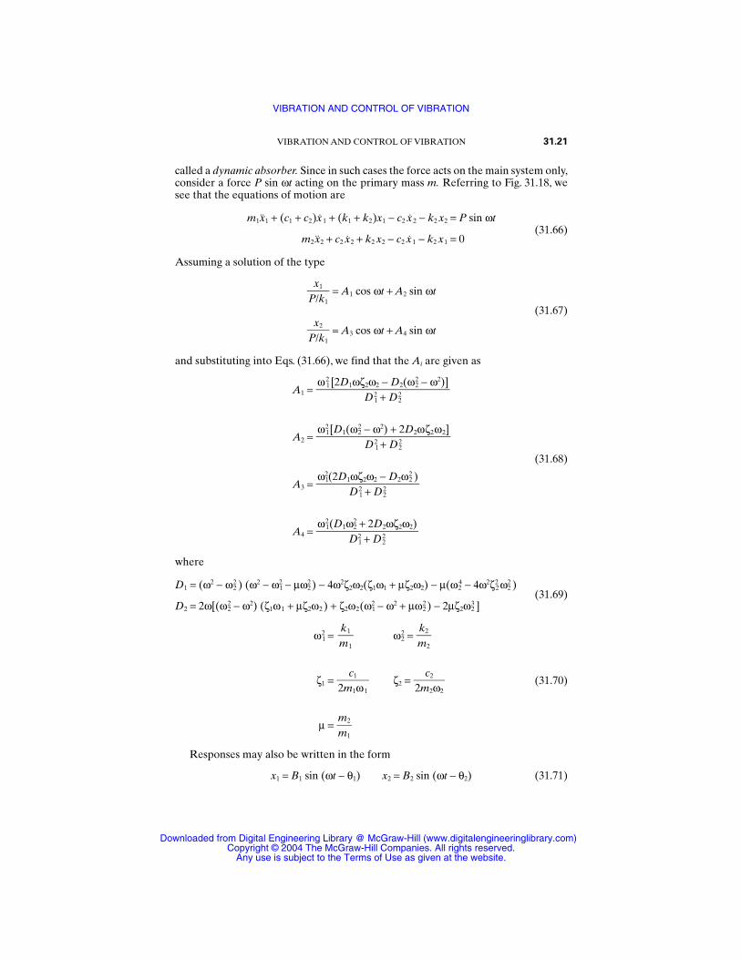
called a dynamic absorber. Since in such cases the force acts on the main system only,consider a force P sin ωt acting on the primary mass m. Referring to Fig. 31.18, wesee that the equations of motion are
m1x1 + (c1 + c2)x1 + (k1 + k2)x1 − c2 x2 − k2 x2 = P sin ωt(31.66)
m2 x2 + c2 x2 + k2 x2 − c2 x1 − k2 x1 = 0
Assuming a solution of the type
= A1 cos ωt + A2 sin ωt
(31.67)
= A3 cos ωt + A4 sin ωt
and substituting into Eqs. (31.66), we find that the Ai are given as
A1 =
A2 =
(31.68)
A3 =
A4 =
where
D1 = (ω2 − ω22 ) (ω2 − ω1
2 − µω22) − 4ω2ζ2ω2(ζ1ω1 + µζ2ω2) − µ(ω2
4 − 4ω2ζ22 ω2
2 )(31.69)
D2 = 2ω[(ω22 − ω2) (ζ1ω 1 + µζ2ω2) + ζ2ω2(ω1
2 − ω2 + µω22) − 2µζ2ω2
3 ]
ω 12 = ω2
2 =
ζ1 = ζ2 = (31.70)
µ =
Responses may also be written in the form
x1 = B1 sin (ωt − θ1) x2 = B2 sin (ωt − θ2) (31.71)
m2m1
c22m2ω2
c12m1ω 1
k2m2
k1m1
ω 12(D1ω2
2 + 2D2ωζ2ω2)
D12 + D2
2
ω12(2D1ωζ2ω2 − D2ω2
2 )
D 12 + D2
2
ω 12 [D1(ω2
2 − ω2) + 2D2ωζ2ω2]
D 12 + D2
2
ω 12 [2D1ωζ2ω2 − D2(ω2
2 − ω2)]
D 12 + D2
2
x2P/k1
x1P/k1
VIBRATION AND CONTROL OF VIBRATION 31.21
VIBRATION AND CONTROL OF VIBRATION
Downloaded from Digital Engineering Library @ McGraw-Hill (www.digitalengineeringlibrary.com)Copyright © 2004 The McGraw-Hill Companies. All rights reserved.
Any use is subject to the Terms of Use as given at the website.
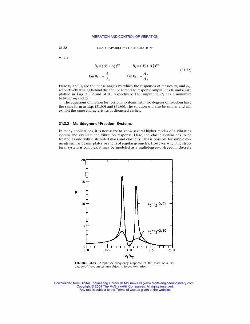
where
B1 = (A12 + A2
2)1/2 B2 = (A32 + A 4
2 )1/2
(31.72)
tan θ1 = − tan θ2 = −
Here θ1 and θ2 are the phase angles by which the responses of masses m1 and m2,respectively, will lag behind the applied force.The response amplitudes B1 and B2 areplotted in Figs. 31.19 and 31.20, respectively. The amplitude B1 has a minimumbetween ω1 and ω2.
The equations of motion for torsional systems with two degrees of freedom havethe same form as Eqs. (31.60) and (31.66). The solution will also be similar and willexhibit the same characteristics as discussed earlier.
31.3.2 Multidegree-of-Freedom Systems
In many applications, it is necessary to know several higher modes of a vibratingsystem and evaluate the vibration response. Here, the elastic system has to betreated as one with distributed mass and elasticity. This is possible for simple ele-ments such as beams, plates, or shells of regular geometry. However, when the struc-tural system is complex, it may be modeled as a multidegree-of-freedom discrete
A 3A 4
A1A2
31.22 LOAD CAPABILITY CONSIDERATIONS
FIGURE 31.19 Amplitude frequency response of the mass of a two-degree-of-freedom system subject to forced excitation.
VIBRATION AND CONTROL OF VIBRATION
Downloaded from Digital Engineering Library @ McGraw-Hill (www.digitalengineeringlibrary.com)Copyright © 2004 The McGraw-Hill Companies. All rights reserved.
Any use is subject to the Terms of Use as given at the website.
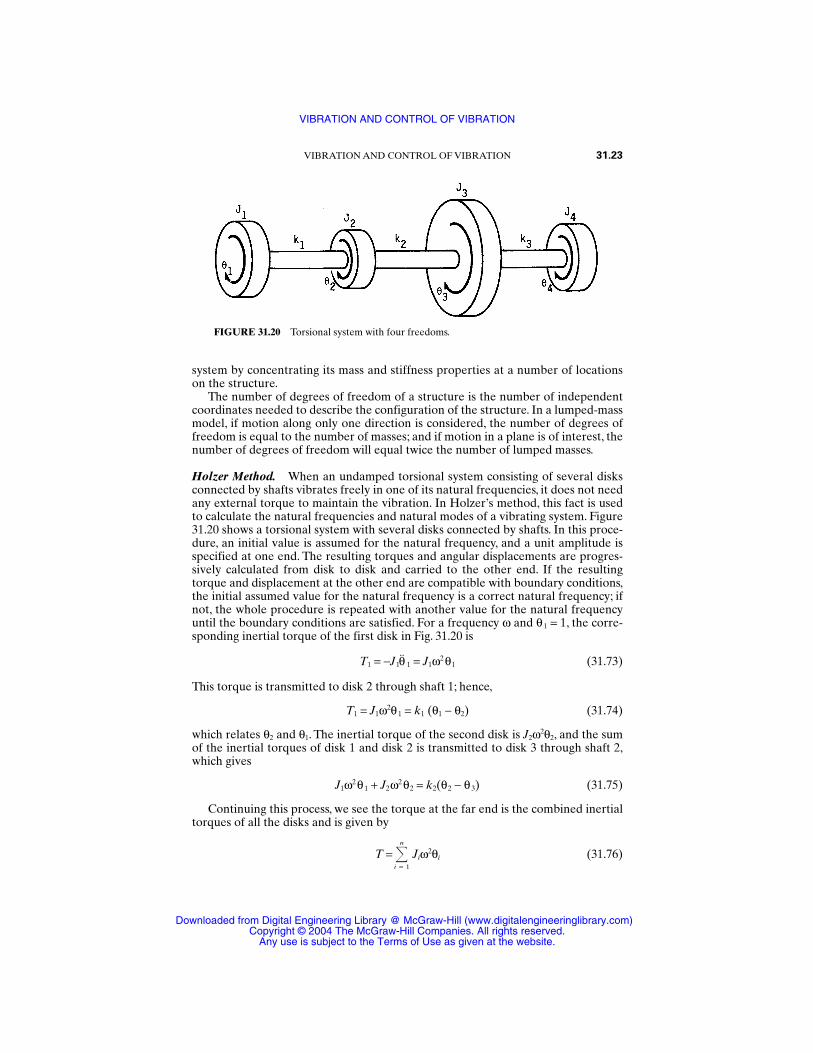
system by concentrating its mass and stiffness properties at a number of locationson the structure.
The number of degrees of freedom of a structure is the number of independentcoordinates needed to describe the configuration of the structure. In a lumped-massmodel, if motion along only one direction is considered, the number of degrees offreedom is equal to the number of masses; and if motion in a plane is of interest, thenumber of degrees of freedom will equal twice the number of lumped masses.
Holzer Method. When an undamped torsional system consisting of several disksconnected by shafts vibrates freely in one of its natural frequencies, it does not needany external torque to maintain the vibration. In Holzer’s method, this fact is usedto calculate the natural frequencies and natural modes of a vibrating system. Figure31.20 shows a torsional system with several disks connected by shafts. In this proce-dure, an initial value is assumed for the natural frequency, and a unit amplitude isspecified at one end. The resulting torques and angular displacements are progres-sively calculated from disk to disk and carried to the other end. If the resultingtorque and displacement at the other end are compatible with boundary conditions,the initial assumed value for the natural frequency is a correct natural frequency; ifnot, the whole procedure is repeated with another value for the natural frequencyuntil the boundary conditions are satisfied. For a frequency ω and θ 1 = 1, the corre-sponding inertial torque of the first disk in Fig. 31.20 is
T1 = −J1θ 1 = J1ω2θ1 (31.73)
This torque is transmitted to disk 2 through shaft 1; hence,
T1 = J1ω2θ 1 = k1 (θ1 − θ2) (31.74)
which relates θ2 and θ1. The inertial torque of the second disk is J2ω2θ2, and the sumof the inertial torques of disk 1 and disk 2 is transmitted to disk 3 through shaft 2,which gives
J1ω2θ 1 + J2ω2θ2 = k2(θ2 − θ 3) (31.75)
Continuing this process, we see the torque at the far end is the combined inertialtorques of all the disks and is given by
T = n
i = 1
Jiω2θi (31.76)
VIBRATION AND CONTROL OF VIBRATION 31.23
FIGURE 31.20 Torsional system with four freedoms.
VIBRATION AND CONTROL OF VIBRATION
Downloaded from Digital Engineering Library @ McGraw-Hill (www.digitalengineeringlibrary.com)Copyright © 2004 The McGraw-Hill Companies. All rights reserved.
Any use is subject to the Terms of Use as given at the website.
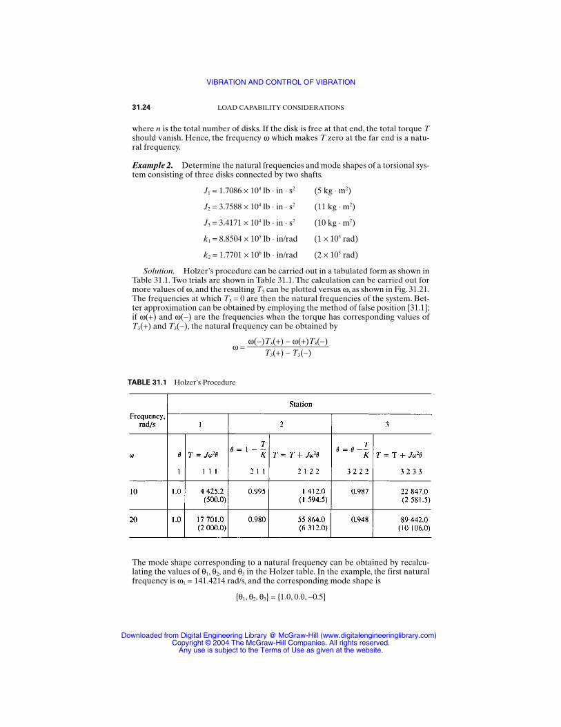
where n is the total number of disks. If the disk is free at that end, the total torque Tshould vanish. Hence, the frequency ω which makes T zero at the far end is a natu-ral frequency.
Example 2. Determine the natural frequencies and mode shapes of a torsional sys-tem consisting of three disks connected by two shafts.
J1 = 1.7086 × 10⁴ lb ⋅ in ⋅ s2 (5 kg ⋅ m2)
J2 = 3.7588 × 10⁴ lb ⋅ in ⋅ s2 (11 kg ⋅ m2)
J3 = 3.4171 × 10⁴ lb ⋅ in ⋅ s2 (10 kg ⋅ m2)
k1 = 8.8504 × 10⁵ lb ⋅ in/rad (1 × 10⁵ rad)
k2 = 1.7701 × 10⁶ lb ⋅ in/rad (2 × 10⁵ rad)
Solution. Holzer’s procedure can be carried out in a tabulated form as shown inTable 31.1. Two trials are shown in Table 31.1. The calculation can be carried out formore values of ω, and the resulting T3 can be plotted versus ω, as shown in Fig. 31.21.The frequencies at which T3 = 0 are then the natural frequencies of the system. Bet-ter approximation can be obtained by employing the method of false position [31.1];if ω(+) and ω(−) are the frequencies when the torque has corresponding values ofT3(+) and T3(−), the natural frequency can be obtained by
ω =ω(−)T3(+) − ω(+)T3(−)
T3(+) − T3(−)
31.24 LOAD CAPABILITY CONSIDERATIONS
TABLE 31.1 Holzer’s Procedure
The mode shape corresponding to a natural frequency can be obtained by recalcu-lating the values of θ1, θ2, and θ3 in the Holzer table. In the example, the first naturalfrequency is ω1 = 141.4214 rad/s, and the corresponding mode shape is
θ1, θ2, θ3 = 1.0, 0.0, −0.5
VIBRATION AND CONTROL OF VIBRATION
Downloaded from Digital Engineering Library @ McGraw-Hill (www.digitalengineeringlibrary.com)Copyright © 2004 The McGraw-Hill Companies. All rights reserved.
Any use is subject to the Terms of Use as given at the website.
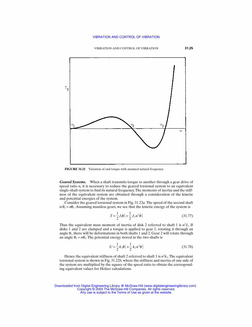
Geared Systems. When a shaft transmits torque to another through a gear drive ofspeed ratio n, it is necessary to reduce the geared torsional system to an equivalentsingle-shaft system to find its natural frequency.The moments of inertia and the stiff-ness of the equivalent system are obtained through a consideration of the kineticand potential energies of the system.
Consider the geared torsional system in Fig. 31.22a. The speed of the second shaftis θ2 = nθ1. Assuming massless gears, we see that the kinetic energy of the system is
T = J1θ 12 + J2 n2 θ 1
2 (31.77)
Thus the equivalent mass moment of inertia of disk 2 referred to shaft 1 is n2J2. Ifdisks 1 and 2 are clamped and a torque is applied to gear 1, rotating it through anangle θ1, there will be deformations in both shafts 1 and 2. Gear 2 will rotate throughan angle θ2 = nθ1. The potential energy stored in the two shafts is
U = k1θ 12 + k2n2θ 1
2 (31.78)
Hence the equivalent stiffness of shaft 2 referred to shaft 1 is n2k2.The equivalenttorsional system is shown in Fig. 31.22b, where the stiffness and inertia of one side ofthe system are multiplied by the square of the speed ratio to obtain the correspond-ing equivalent values for Holzer calculations.
12
12
12
12
VIBRATION AND CONTROL OF VIBRATION 31.25
FIGURE 31.21 Variation of end torque with assumed natural frequency.
VIBRATION AND CONTROL OF VIBRATION
Downloaded from Digital Engineering Library @ McGraw-Hill (www.digitalengineeringlibrary.com)Copyright © 2004 The McGraw-Hill Companies. All rights reserved.
Any use is subject to the Terms of Use as given at the website.
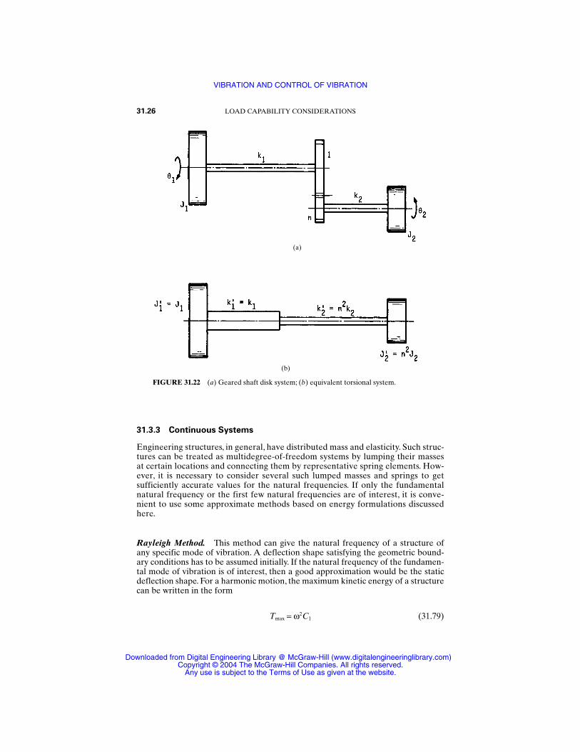
31.3.3 Continuous Systems
Engineering structures, in general, have distributed mass and elasticity. Such struc-tures can be treated as multidegree-of-freedom systems by lumping their masses at certain locations and connecting them by representative spring elements. How-ever, it is necessary to consider several such lumped masses and springs to get sufficiently accurate values for the natural frequencies. If only the fundamentalnatural frequency or the first few natural frequencies are of interest, it is conve-nient to use some approximate methods based on energy formulations discussedhere.
Rayleigh Method. This method can give the natural frequency of a structure ofany specific mode of vibration. A deflection shape satisfying the geometric bound-ary conditions has to be assumed initially. If the natural frequency of the fundamen-tal mode of vibration is of interest, then a good approximation would be the staticdeflection shape. For a harmonic motion, the maximum kinetic energy of a structurecan be written in the form
Tmax = ω2C1 (31.79)
31.26 LOAD CAPABILITY CONSIDERATIONS
FIGURE 31.22 (a) Geared shaft disk system; (b) equivalent torsional system.
(a)
(b)
VIBRATION AND CONTROL OF VIBRATION
Downloaded from Digital Engineering Library @ McGraw-Hill (www.digitalengineeringlibrary.com)Copyright © 2004 The McGraw-Hill Companies. All rights reserved.
Any use is subject to the Terms of Use as given at the website.
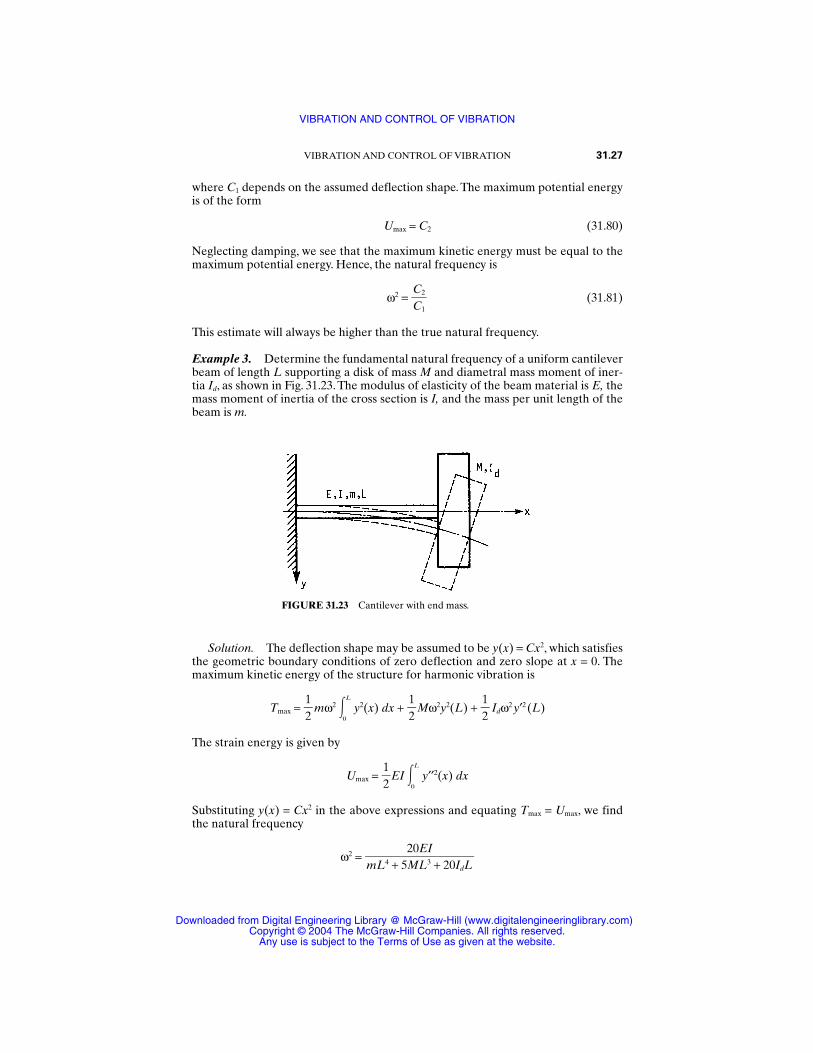
where C1 depends on the assumed deflection shape. The maximum potential energyis of the form
Umax = C2 (31.80)
Neglecting damping, we see that the maximum kinetic energy must be equal to themaximum potential energy. Hence, the natural frequency is
ω2 = (31.81)
This estimate will always be higher than the true natural frequency.
Example 3. Determine the fundamental natural frequency of a uniform cantileverbeam of length L supporting a disk of mass M and diametral mass moment of iner-tia Id, as shown in Fig. 31.23. The modulus of elasticity of the beam material is E, themass moment of inertia of the cross section is I, and the mass per unit length of thebeam is m.
C2C1
VIBRATION AND CONTROL OF VIBRATION 31.27
FIGURE 31.23 Cantilever with end mass.
Solution. The deflection shape may be assumed to be y(x) = Cx2, which satisfiesthe geometric boundary conditions of zero deflection and zero slope at x = 0. Themaximum kinetic energy of the structure for harmonic vibration is
Tmax = mω2 L
0
y2(x) dx + Mω2y2(L) + Idω2y′2(L)
The strain energy is given by
Umax = EI L
0
y′′2(x) dx
Substituting y(x) = Cx2 in the above expressions and equating Tmax = Umax, we findthe natural frequency
ω2 =20EI
mL4 + 5ML3 + 20IdL
12
12
12
12
VIBRATION AND CONTROL OF VIBRATION
Downloaded from Digital Engineering Library @ McGraw-Hill (www.digitalengineeringlibrary.com)Copyright © 2004 The McGraw-Hill Companies. All rights reserved.
Any use is subject to the Terms of Use as given at the website.
In the absence of the disk, ω = 4.47 (EI/mL4)1/2. By comparing this to the exact resultω = 3.52 (EI/mL4)1/2, the error in the approximation is error = 0.95 (EI/mL4)1/2, or26.9 percent.
This error can be reduced by obtaining the strain energy by using a differentmethod.The shear at any section is obtained by integrating the inertial loading fromthe free end as
V(ξ) = ω2 L
ξm(ξ)y(ξ) dξ + Mω2y(L)
= ω2mc(L3 − ξ3) + Mω2cL2
and the moment at any point x is
M(x) = L
x
V(ξ) dξ + Idy′(L) = ω2mc(3L4 − 4L3x + x4) + Mω2cL2(L − x) + 2IdcL
The strain energy is then
Umax = L
0
dx
When the disk is absent,
Umax = L9
With Tmax and Umax equated, the natural frequency ω = 3.53 (EI/ML4)1/2 has an errorof only 0.28 percent.
31.4 VIBRATION ISOLATION
Often machines and components which exhibit vibrations have to be mounted inlocations where vibrations may not be desirable.Then the machine has to be isolatedproperly so that it does not transmit vibrations.
31.4.1 Transmissibility
Active Isolation and Transmissibility. From Eq. (31.38), the force transmissibility,which is the magnitude of the ratio of the force transmitted to the force applied, isgiven by
T = 1/2
(31.82)
Equation (31.82) is plotted in Fig. 31.12 for different values of . All the curves crossat /n = 2. For /n 2, transmissibility, although below unity, increases with
1 + (2 n)2
(1 − 2/n
2)2 + (2/n)2
312135
m2c2
144
ω4
2EI
M 2(x)
EI12
112
13
31.28 LOAD CAPABILITY CONSIDERATIONS
VIBRATION AND CONTROL OF VIBRATION
Downloaded from Digital Engineering Library @ McGraw-Hill (www.digitalengineeringlibrary.com)Copyright © 2004 The McGraw-Hill Companies. All rights reserved.
Any use is subject to the Terms of Use as given at the website.
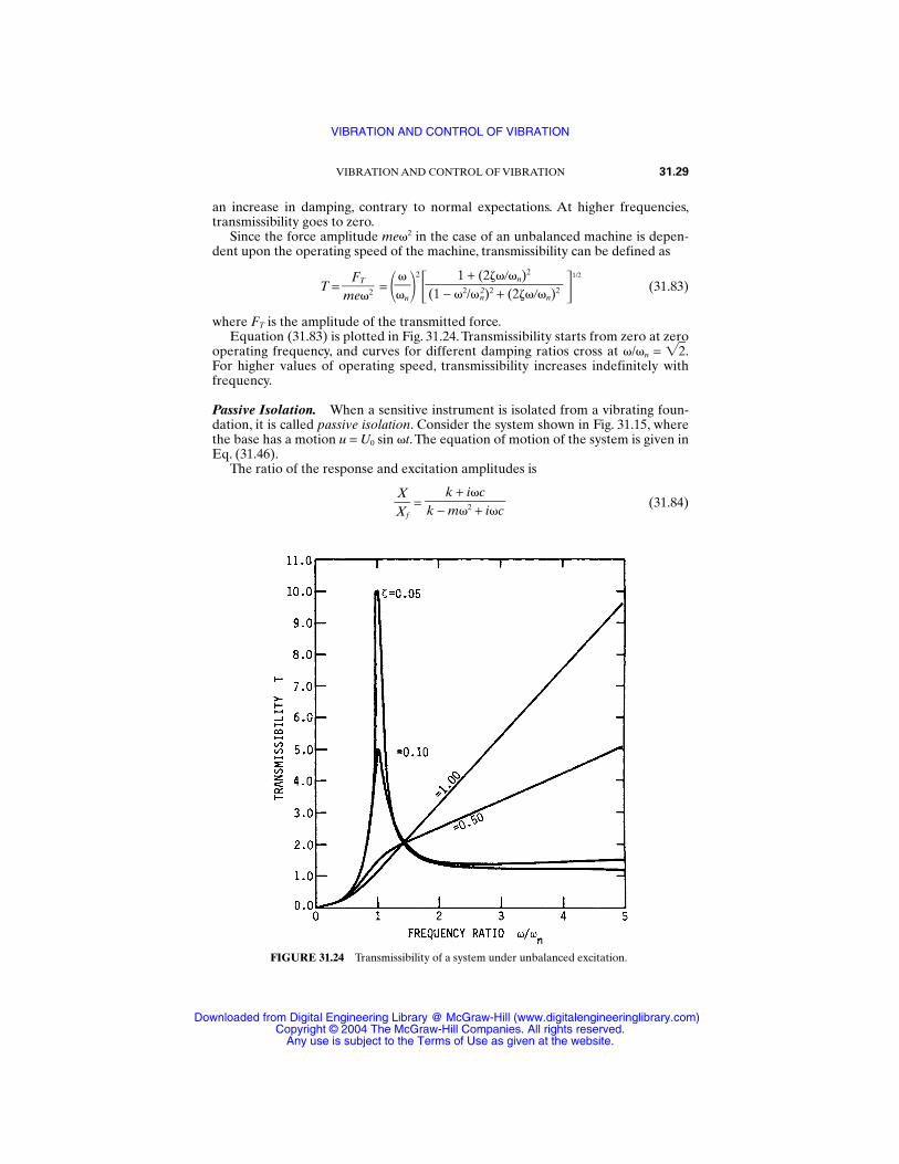
an increase in damping, contrary to normal expectations. At higher frequencies,transmissibility goes to zero.
Since the force amplitude me2 in the case of an unbalanced machine is depen-dent upon the operating speed of the machine, transmissibility can be defined as
T = = 2
1/2
(31.83)
where FT is the amplitude of the transmitted force.Equation (31.83) is plotted in Fig. 31.24. Transmissibility starts from zero at zero
operating frequency, and curves for different damping ratios cross at /n = 2.For higher values of operating speed, transmissibility increases indefinitely withfrequency.
Passive Isolation. When a sensitive instrument is isolated from a vibrating foun-dation, it is called passive isolation. Consider the system shown in Fig. 31.15, wherethe base has a motion u = U0 sin t. The equation of motion of the system is given inEq. (31.46).
The ratio of the response and excitation amplitudes is
= (31.84)k + ic
k − m2 + ic
XXf
1 + (2 n)2
(1 − 2/n
2)2 + (2 n)2
n
FTme2
VIBRATION AND CONTROL OF VIBRATION 31.29
FIGURE 31.24 Transmissibility of a system under unbalanced excitation.
VIBRATION AND CONTROL OF VIBRATION
Downloaded from Digital Engineering Library @ McGraw-Hill (www.digitalengineeringlibrary.com)Copyright © 2004 The McGraw-Hill Companies. All rights reserved.
Any use is subject to the Terms of Use as given at the website.

Since we are interested in the motion transmissibility in the case of passive isolation,Eq. (31.84) gives the transmissibility T, which can be put in terms of nondimensionalparameters, as
T = 1/2
(31.85)
Equation (31.85) is identical to the force transmissibility in the case of active isola-tion given in Eq. (31.82).
REFERENCES
31.1 R. L. Burden, J. D. Faires, and A. C. Reynolds, Numerical Analysis, 2d ed., Prindle,Weberand Schmidt, Boston, 1981.
31.2 R. B. Bhat, J. S. Rao, and T. S. Sankar, “Optimum Journal Bearing Parameters for Mini-mum Unbalance Response in Synchronous Whirl,” ASME Design Engineering Confer-ence, Paper No. 81-DET-55, 1981. (To be published in ASME Transactions.)
31.3 J. P. Den Hartog, Mechanical Vibrations, McGraw-Hill, New York, 1962.
31.4 W. T. Thomson, Theory of Vibration with Applications, Prentice-Hall, Englewood Cliffs,N.J., 1981.
31.5 T. S. Sankar and G. D. Xistris, “Failure Prediction through the Theory of StochasticExcursions of Extreme Vibration Amplitudes,” J. Eng. Ind., Trans. ASME, 1972.
31.6 NASTRAN Computer Program, McNeil Schwendler Corporation, Los Angeles.
31.7 ANSYS Computer Program, SWANSON Analysis Systems Incorporated, Houston,Pennsylvania.
31.8 ADINA Computer Program, ADINA Engineering AB VASTERAS, Sweden.
31.9 SPAR Structural Analysis System, Engineering Information Systems, Inc., San Jose, Cal-ifornia.
31.10 PROSSS—Programming Structural Synthesis System, NASA Langley Research Center,Hampton, Virginia.
1 + (2 n)2
(1 − 2/n
2)2 + (2/n)2
XU0
31.30 LOAD CAPABILITY CONSIDERATIONS
VIBRATION AND CONTROL OF VIBRATION
Downloaded from Digital Engineering Library @ McGraw-Hill (www.digitalengineeringlibrary.com)Copyright © 2004 The McGraw-Hill Companies. All rights reserved.
Any use is subject to the Terms of Use as given at the website.

P • A • R • T • 8
PERFORMANCE OFENGINEERING
MATERIALS
Source: STANDARD HANDBOOK OF MACHINE DESIGN
Downloaded from Digital Engineering Library @ McGraw-Hill (www.digitalengineeringlibrary.com)Copyright © 2004 The McGraw-Hill Companies. All rights reserved.
Any use is subject to the Terms of Use as given at the website.

PERFORMANCE OF ENGINEERING MATERIALS
Downloaded from Digital Engineering Library @ McGraw-Hill (www.digitalengineeringlibrary.com)Copyright © 2004 The McGraw-Hill Companies. All rights reserved.
Any use is subject to the Terms of Use as given at the website.
CHAPTER 32SOLID MATERIALS
Joseph DatskoProfessor Emeritus of Mechanical Engineering
The University of MichiganAnn Arbor, Michigan
32.1 STRUCTURE OF SOLIDS / 32.3
32.2 ATOMIC BONDING FORCES / 32.4
32.3 ATOMIC STRUCTURES / 32.6
32.4 CRYSTAL IMPERFECTIONS / 32.13
32.5 SLIP IN CRYSTALLINE SOLIDS / 32.17
32.6 MECHANICAL STRENGTH / 32.19
32.7 MECHANICAL PROPERTIES AND TESTS / 32.22
32.8 HARDNESS / 32.23
32.9 THE TENSILE TEST / 32.27
32.10 TENSILE PROPERTIES / 32.34
32.11 STRENGTH, STRESS, AND STRAIN RELATIONS / 32.38
32.12 IMPACT STRENGTH / 32.44
32.13 CREEP STRENGTH / 32.45
32.14 MECHANICAL-PROPERTY DATA / 32.48
32.15 NUMBERING SYSTEMS / 32.53
REFERENCES / 32.57
This chapter summarizes the structure of solids, including atomic bonding forces,atomic structures, crystal imperfections, slip, and mechanical strength.The section onmechanical properties and tests discusses all the hardness tests and includes adetailed explanation of the tensile test and tensile properties. The section onstrength, stress, and strain relations includes many new relationships that have beendeveloped during the past two decades and are not found in other handbooks. Themechanical property data presented in this section are in a new format that is wellsuited for use in computer-aided-engineering (CAE) applications.
32.1 STRUCTURE OF SOLIDS
A study of the mechanical properties of materials must begin with an understandingof the structure of solid materials. In this context, structure refers to the atomisticand crystalline patterns of which the solid material is composed. The definitions ofthe mechanical properties given in the following sections are on the basis of the crys-talline structure of material. For example, strength (and hardness) is defined as theability of the material to resist slip along its crystallographic planes.Thus, in order toincrease the strength of a material, something must be done to it which will make
32.3
Source: STANDARD HANDBOOK OF MACHINE DESIGN
Downloaded from Digital Engineering Library @ McGraw-Hill (www.digitalengineeringlibrary.com)Copyright © 2004 The McGraw-Hill Companies. All rights reserved.
Any use is subject to the Terms of Use as given at the website.
slip more difficult to initiate.The following sections will explain the manner in whichthe various thermal and mechanical processes affect the structure of a material,which in turn determines the mechanical properties. The next section presents abrief review of atomic structure.
32.2 ATOMIC BONDING FORCES
The smallest particles that must be considered in the preceding context are atoms.The manner in which atoms are arranged in a solid material determines the mate-rial’s crystal structure. The crystal structure and the type of interatomic bondingforces determine the strength and ductility of the material.
The simple model of an atom is a dense nucleus, consisting of protons and neu-trons, surrounded by discrete numbers of planetary electrons orbiting in shells atspecific distances from the nucleus. Each proton has a positive electric charge ofunity (1+). The number of protons in the nucleus determines the nuclear charge ofthe atom and is called the atomic number. The neutrons have no charge, but they dohave mass. The atomic weight of an atom is the sum of the number of protons andneutrons.The electrons have negligible mass and a negative charge of unity (1−).Thenumber of electrons in a given type of atom is also equal to the atomic number ofthat element. The maximum number of electrons in any shell is 2n2, where n is thequantum number of the shell. Thus the maximum number of electrons that can bepresent in the first (innermost) shell is 2, and 8 is the maximum in the second shell.However, no more than 8 electrons are ever present in the outermost shell of anatom. The valence of an element is either the number of electrons in its outermostshell or the number of electrons necessary to fill that shell, whichever number islower.
The interatomic bonding forces are determined by the valence, or outer-shell,electrons. There are four types of atomic bonding forces that hold the atoms of asolid material in their relatively fixed positions. The three strongest (ionic, covalent,and metallic) types of bond are referred to as primary; the fourth (molecular) isreferred to as a secondary type of bond.
32.2.1 Ionic Bonds
From the preceding brief description of atomic structure, it is evident that theuncombined atom is electrically neutral—the number of protons (+ charges) in thenucleus exactly equals the number of electrons (− charges). When atoms combine,only the valence electrons are involved and not the nuclei. When a metal combineswith a nonmetal, each metal atom “loses” its valence electrons and thus acquires apositive charge that is equal to the number of electrons so lost. Likewise each non-metallic atom “gains” a number of electrons equal to its valence and acquires anequal negative charge. While in this state, the positively charged metallic atom andthe negatively charged nonmetallic atom are called ions.
Like-charged particles repel each other and oppositely charged particles attracteach other with an electric force called the Coulomb force. When a material is main-tained in the solid state by the mutual attraction of positively and negatively chargedions, the interatomic bonding force is called ionic.
The Coulomb forces attracting oppositely charged ions are very large.Therefore,ionic-bonded solids exhibit very high strength and relatively low melting tempera-
32.4 PERFORMANCE OF ENGINEERING MATERIALS
SOLID MATERIALS
Downloaded from Digital Engineering Library @ McGraw-Hill (www.digitalengineeringlibrary.com)Copyright © 2004 The McGraw-Hill Companies. All rights reserved.
Any use is subject to the Terms of Use as given at the website.
tures. However, they exhibit very low ductility under normal conditions because theinteratomic bonds must be broken in order for the atoms to slide past each other.This is one of the most important distinctions between ionic (or covalent) bondingand metallic bonding and is discussed later.
32.2.2 Covalent Bonds
Covalent bonds are those in which the atoms reach a stable configuration (filledouter shell) by sharing valence electrons. Unlike ionic bonds, which are nondirec-tional, covalent bonds act between specific pairs of atoms and thus form mole-cules. Covalent bonds are most prevalent in gas molecules. Covalent bonding alsoresults in the formation of very large molecules which are present as solids ratherthan as liquids and gases. Diamond, silicon, and silicon carbide are examples ofsuch covalent-bonded solids. They are characterized by high strength and meltingtemperature and low ductility.The atoms in the diamond structure are arranged ontwo interpenetrating face-centered cubic lattices. The entire crystal is composed ofonly one molecule, and in order to fracture the crystal, the strong covalent inter-atomic bonds must be broken.
32.2.3 Metallic Bonds
Of the three primary bonding forces, the metallic bond is by far the most importantfor an understanding of the mechanical properties of the materials with which thepracticing engineer is concerned.The metallic bond is a special type of covalent bondwherein the positively charged nuclei of the metal atoms are attracted by electro-static forces to the valence electrons that surround them. Unlike the common cova-lent bond, which is directional, i.e., between a pair of atoms, the metallic bond isnondirectional, and each nucleus attracts as many valence electrons as possible.Thisleads to a dense packing of the atoms, and thus the most common crystal structuresof the metals are the close-packed ones: face- and body-centered cubic and hexago-nal close-packed structures.
The reason that metal atoms have their own unique type of bonding force is thelooseness with which their valence electrons are held in the outer shell. This is evi-dent from the fact that the ionization potential of metal atoms is one-half to two-thirds that of nonmetal atoms. The mean radius of the valence electrons in a free(isolated) metal atom is larger than the interatomic distance of that metal in thesolid crystalline state. This means that the valence electrons are closer to a nucleusin the solid metal than they are in a free atom, and thus their potential energy islower in the solid.
Since the valence electrons are not localized between a pair of positive ions, theyare free to move through the solid. Thus the structure of the solid metal is a close-packed arrangement of positive ion “cores” (the nucleus plus the nonvalence elec-trons) that is permeated by an electron “gas” or “cloud.” This ability of the valenceelectrons to move freely through the solid explains the high thermal and electricalconductivities of metals. Also, the fact that the valence electrons are nondirectional(not shared by only two atoms) explains the relatively low strength and high ductil-ity of elemental metals, since the positive ions can move relative to one anotherwithout breaking any primary bonds.This mechanism is referred to as slip and is dis-cussed in more detail in a following section on crystal structures.
SOLID MATERIALS 32.5
SOLID MATERIALS
Downloaded from Digital Engineering Library @ McGraw-Hill (www.digitalengineeringlibrary.com)Copyright © 2004 The McGraw-Hill Companies. All rights reserved.
Any use is subject to the Terms of Use as given at the website.
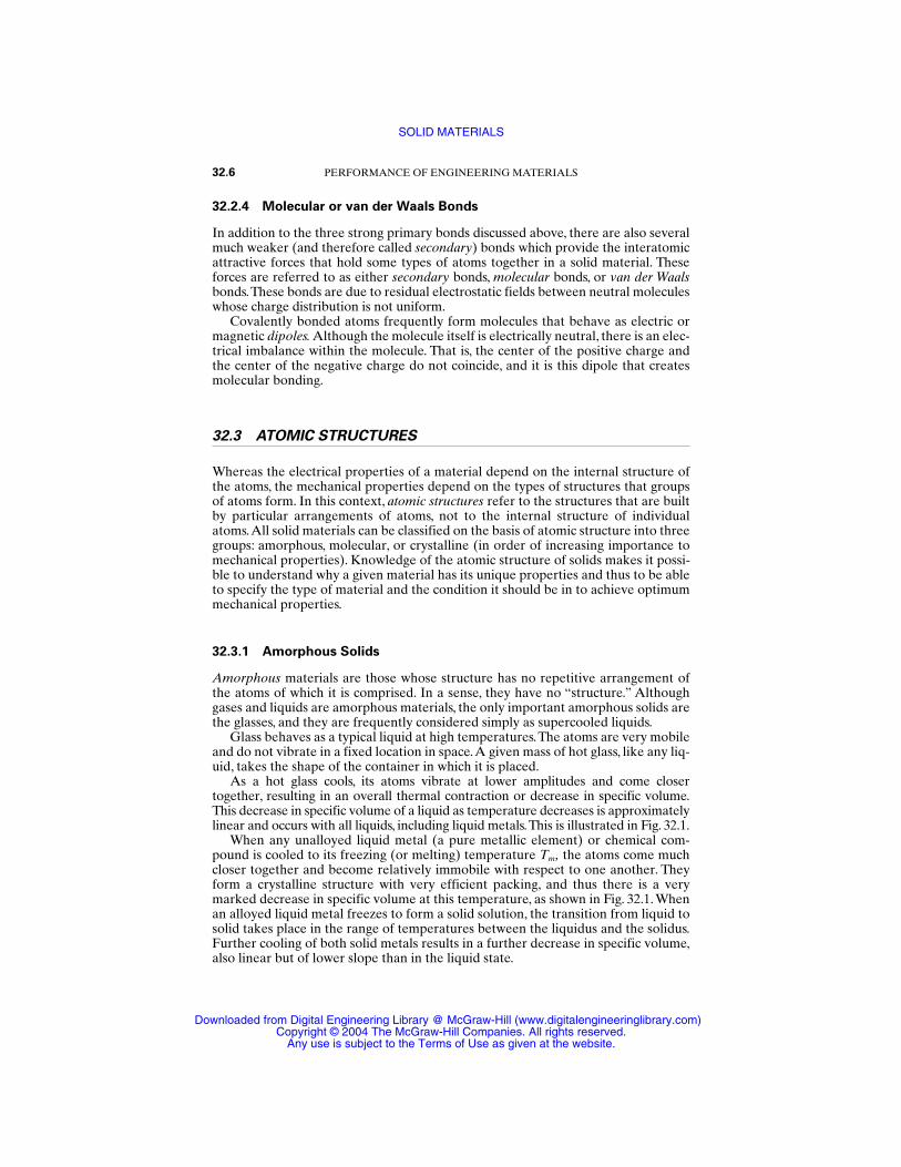
32.2.4 Molecular or van der Waals Bonds
In addition to the three strong primary bonds discussed above, there are also severalmuch weaker (and therefore called secondary) bonds which provide the interatomicattractive forces that hold some types of atoms together in a solid material. Theseforces are referred to as either secondary bonds, molecular bonds, or van der Waalsbonds.These bonds are due to residual electrostatic fields between neutral moleculeswhose charge distribution is not uniform.
Covalently bonded atoms frequently form molecules that behave as electric ormagnetic dipoles. Although the molecule itself is electrically neutral, there is an elec-trical imbalance within the molecule. That is, the center of the positive charge andthe center of the negative charge do not coincide, and it is this dipole that createsmolecular bonding.
32.3 ATOMIC STRUCTURES
Whereas the electrical properties of a material depend on the internal structure ofthe atoms, the mechanical properties depend on the types of structures that groupsof atoms form. In this context, atomic structures refer to the structures that are builtby particular arrangements of atoms, not to the internal structure of individualatoms.All solid materials can be classified on the basis of atomic structure into threegroups: amorphous, molecular, or crystalline (in order of increasing importance tomechanical properties). Knowledge of the atomic structure of solids makes it possi-ble to understand why a given material has its unique properties and thus to be ableto specify the type of material and the condition it should be in to achieve optimummechanical properties.
32.3.1 Amorphous Solids
Amorphous materials are those whose structure has no repetitive arrangement ofthe atoms of which it is comprised. In a sense, they have no “structure.” Althoughgases and liquids are amorphous materials, the only important amorphous solids arethe glasses, and they are frequently considered simply as supercooled liquids.
Glass behaves as a typical liquid at high temperatures.The atoms are very mobileand do not vibrate in a fixed location in space.A given mass of hot glass, like any liq-uid, takes the shape of the container in which it is placed.
As a hot glass cools, its atoms vibrate at lower amplitudes and come closertogether, resulting in an overall thermal contraction or decrease in specific volume.This decrease in specific volume of a liquid as temperature decreases is approximatelylinear and occurs with all liquids, including liquid metals.This is illustrated in Fig. 32.1.
When any unalloyed liquid metal (a pure metallic element) or chemical com-pound is cooled to its freezing (or melting) temperature Tm, the atoms come muchcloser together and become relatively immobile with respect to one another. Theyform a crystalline structure with very efficient packing, and thus there is a verymarked decrease in specific volume at this temperature, as shown in Fig. 32.1. Whenan alloyed liquid metal freezes to form a solid solution, the transition from liquid tosolid takes place in the range of temperatures between the liquidus and the solidus.Further cooling of both solid metals results in a further decrease in specific volume,also linear but of lower slope than in the liquid state.
32.6 PERFORMANCE OF ENGINEERING MATERIALS
SOLID MATERIALS
Downloaded from Digital Engineering Library @ McGraw-Hill (www.digitalengineeringlibrary.com)Copyright © 2004 The McGraw-Hill Companies. All rights reserved.
Any use is subject to the Terms of Use as given at the website.
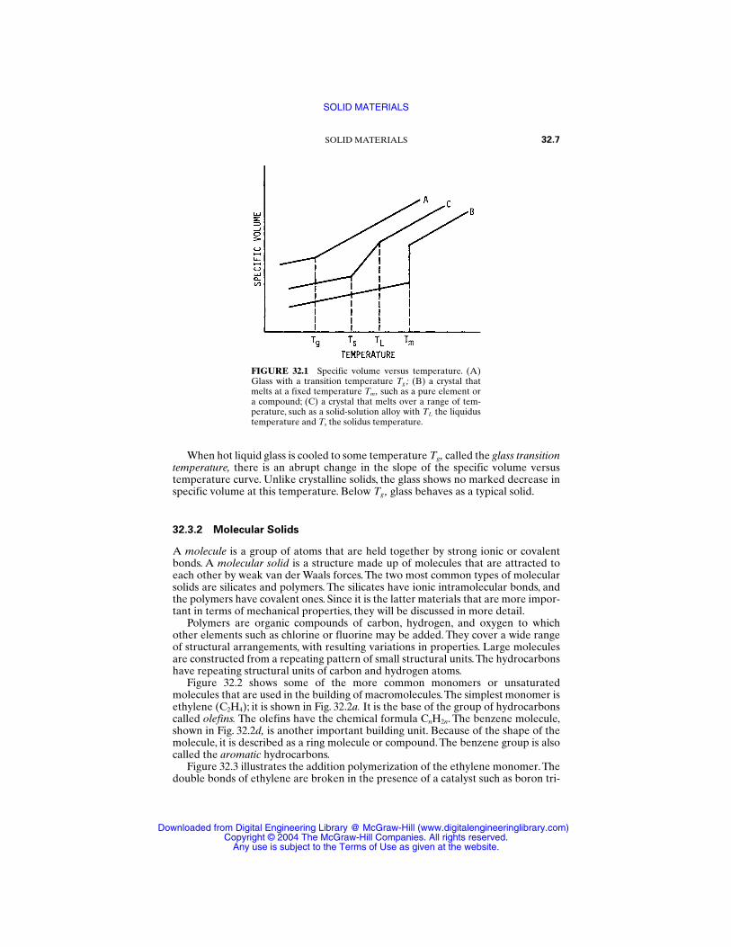
When hot liquid glass is cooled to some temperature Tg, called the glass transitiontemperature, there is an abrupt change in the slope of the specific volume versustemperature curve. Unlike crystalline solids, the glass shows no marked decrease inspecific volume at this temperature. Below Tg, glass behaves as a typical solid.
32.3.2 Molecular Solids
A molecule is a group of atoms that are held together by strong ionic or covalentbonds. A molecular solid is a structure made up of molecules that are attracted toeach other by weak van der Waals forces. The two most common types of molecularsolids are silicates and polymers. The silicates have ionic intramolecular bonds, andthe polymers have covalent ones. Since it is the latter materials that are more impor-tant in terms of mechanical properties, they will be discussed in more detail.
Polymers are organic compounds of carbon, hydrogen, and oxygen to whichother elements such as chlorine or fluorine may be added. They cover a wide rangeof structural arrangements, with resulting variations in properties. Large moleculesare constructed from a repeating pattern of small structural units.The hydrocarbonshave repeating structural units of carbon and hydrogen atoms.
Figure 32.2 shows some of the more common monomers or unsaturatedmolecules that are used in the building of macromolecules.The simplest monomer isethylene (C2H4); it is shown in Fig. 32.2a. It is the base of the group of hydrocarbonscalled olefins. The olefins have the chemical formula CnH2n. The benzene molecule,shown in Fig. 32.2d, is another important building unit. Because of the shape of themolecule, it is described as a ring molecule or compound. The benzene group is alsocalled the aromatic hydrocarbons.
Figure 32.3 illustrates the addition polymerization of the ethylene monomer.Thedouble bonds of ethylene are broken in the presence of a catalyst such as boron tri-
SOLID MATERIALS 32.7
FIGURE 32.1 Specific volume versus temperature. (A)Glass with a transition temperature Tg ; (B) a crystal thatmelts at a fixed temperature Tm, such as a pure element ora compound; (C) a crystal that melts over a range of tem-perature, such as a solid-solution alloy with TL the liquidustemperature and Ts the solidus temperature.
SOLID MATERIALS
Downloaded from Digital Engineering Library @ McGraw-Hill (www.digitalengineeringlibrary.com)Copyright © 2004 The McGraw-Hill Companies. All rights reserved.
Any use is subject to the Terms of Use as given at the website.
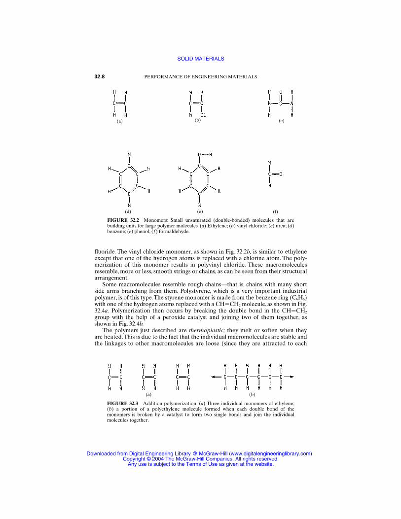
fluoride. The vinyl chloride monomer, as shown in Fig. 32.2b, is similar to ethyleneexcept that one of the hydrogen atoms is replaced with a chlorine atom. The poly-merization of this monomer results in polyvinyl chloride. These macromoleculesresemble, more or less, smooth strings or chains, as can be seen from their structuralarrangement.
Some macromolecules resemble rough chains—that is, chains with many shortside arms branching from them. Polystyrene, which is a very important industrialpolymer, is of this type.The styrene monomer is made from the benzene ring (C6H6)with one of the hydrogen atoms replaced with a CHCH2 molecule, as shown in Fig.32.4a. Polymerization then occurs by breaking the double bond in the CHCH2
group with the help of a peroxide catalyst and joining two of them together, asshown in Fig. 32.4b.
The polymers just described are thermoplastic; they melt or soften when theyare heated.This is due to the fact that the individual macromolecules are stable andthe linkages to other macromolecules are loose (since they are attracted to each
32.8 PERFORMANCE OF ENGINEERING MATERIALS
FIGURE 32.2 Monomers: Small unsaturated (double-bonded) molecules that arebuilding units for large polymer molecules. (a) Ethylene; (b) vinyl chloride; (c) urea; (d)benzene; (e) phenol; (f) formaldehyde.
(d) (e) (f)
(a) (b) (c)
FIGURE 32.3 Addition polymerization. (a) Three individual monomers of ethylene;(b) a portion of a polyethylene molecule formed when each double bond of themonomers is broken by a catalyst to form two single bonds and join the individualmolecules together.
(a) (b)
SOLID MATERIALS
Downloaded from Digital Engineering Library @ McGraw-Hill (www.digitalengineeringlibrary.com)Copyright © 2004 The McGraw-Hill Companies. All rights reserved.
Any use is subject to the Terms of Use as given at the website.
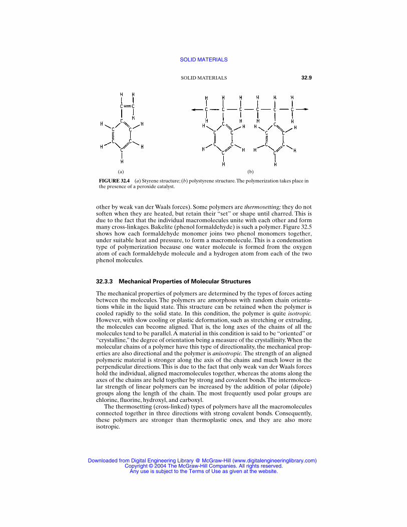
other by weak van der Waals forces). Some polymers are thermosetting; they do notsoften when they are heated, but retain their “set” or shape until charred. This isdue to the fact that the individual macromolecules unite with each other and formmany cross-linkages. Bakelite (phenol formaldehyde) is such a polymer. Figure 32.5shows how each formaldehyde monomer joins two phenol monomers together,under suitable heat and pressure, to form a macromolecule. This is a condensationtype of polymerization because one water molecule is formed from the oxygenatom of each formaldehyde molecule and a hydrogen atom from each of the twophenol molecules.
32.3.3 Mechanical Properties of Molecular Structures
The mechanical properties of polymers are determined by the types of forces actingbetween the molecules. The polymers are amorphous with random chain orienta-tions while in the liquid state. This structure can be retained when the polymer iscooled rapidly to the solid state. In this condition, the polymer is quite isotropic.However, with slow cooling or plastic deformation, such as stretching or extruding,the molecules can become aligned. That is, the long axes of the chains of all themolecules tend to be parallel. A material in this condition is said to be “oriented” or“crystalline,” the degree of orientation being a measure of the crystallinity.When themolecular chains of a polymer have this type of directionality, the mechanical prop-erties are also directional and the polymer is anisotropic. The strength of an alignedpolymeric material is stronger along the axis of the chains and much lower in theperpendicular directions. This is due to the fact that only weak van der Waals forceshold the individual, aligned macromolecules together, whereas the atoms along theaxes of the chains are held together by strong and covalent bonds. The intermolecu-lar strength of linear polymers can be increased by the addition of polar (dipole)groups along the length of the chain. The most frequently used polar groups arechlorine, fluorine, hydroxyl, and carboxyl.
The thermosetting (cross-linked) types of polymers have all the macromoleculesconnected together in three directions with strong covalent bonds. Consequently,these polymers are stronger than thermoplastic ones, and they are also moreisotropic.
SOLID MATERIALS 32.9
FIGURE 32.4 (a) Styrene structure; (b) polystyrene structure.The polymerization takes place inthe presence of a peroxide catalyst.
(a) (b)
SOLID MATERIALS
Downloaded from Digital Engineering Library @ McGraw-Hill (www.digitalengineeringlibrary.com)Copyright © 2004 The McGraw-Hill Companies. All rights reserved.
Any use is subject to the Terms of Use as given at the website.
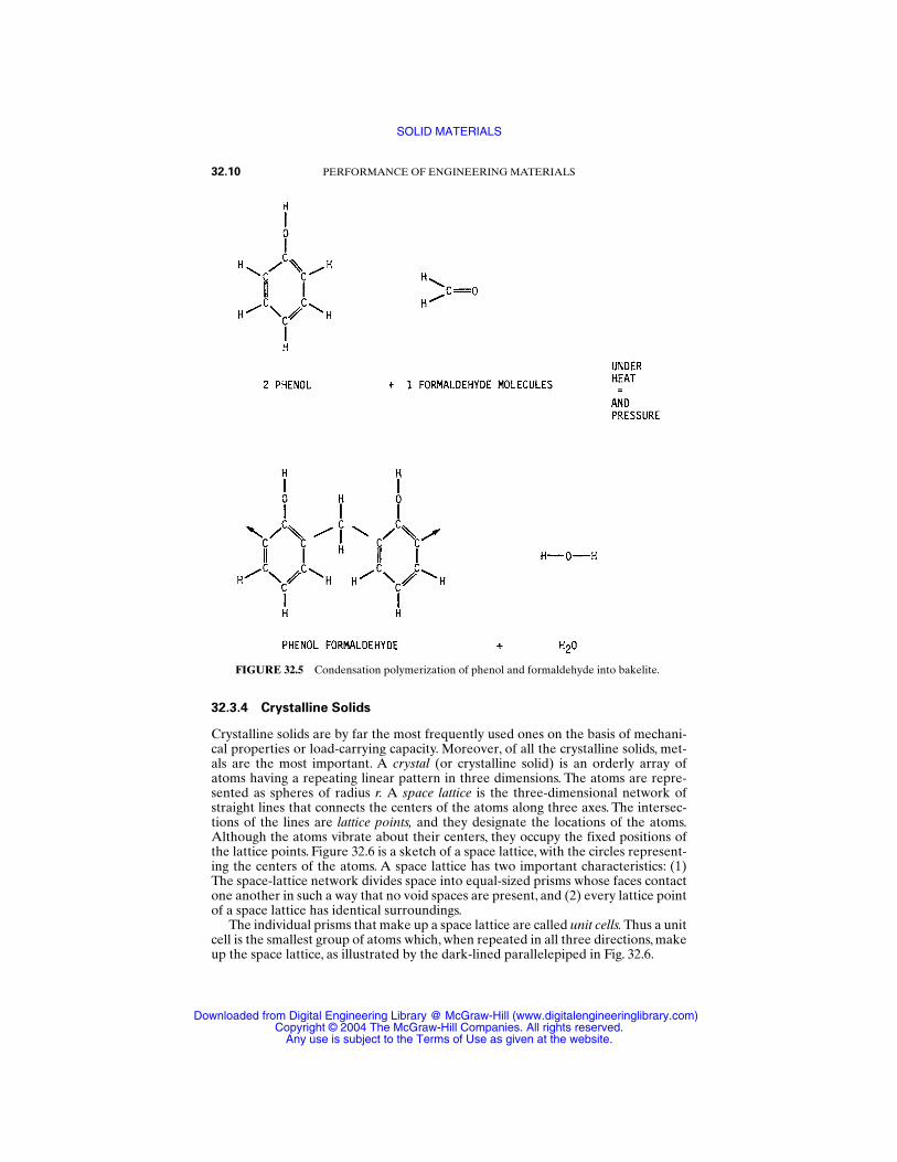
32.3.4 Crystalline Solids
Crystalline solids are by far the most frequently used ones on the basis of mechani-cal properties or load-carrying capacity. Moreover, of all the crystalline solids, met-als are the most important. A crystal (or crystalline solid) is an orderly array ofatoms having a repeating linear pattern in three dimensions. The atoms are repre-sented as spheres of radius r. A space lattice is the three-dimensional network ofstraight lines that connects the centers of the atoms along three axes. The intersec-tions of the lines are lattice points, and they designate the locations of the atoms.Although the atoms vibrate about their centers, they occupy the fixed positions ofthe lattice points. Figure 32.6 is a sketch of a space lattice, with the circles represent-ing the centers of the atoms. A space lattice has two important characteristics: (1)The space-lattice network divides space into equal-sized prisms whose faces contactone another in such a way that no void spaces are present, and (2) every lattice pointof a space lattice has identical surroundings.
The individual prisms that make up a space lattice are called unit cells. Thus a unitcell is the smallest group of atoms which, when repeated in all three directions, makeup the space lattice, as illustrated by the dark-lined parallelepiped in Fig. 32.6.
32.10 PERFORMANCE OF ENGINEERING MATERIALS
FIGURE 32.5 Condensation polymerization of phenol and formaldehyde into bakelite.
SOLID MATERIALS
Downloaded from Digital Engineering Library @ McGraw-Hill (www.digitalengineeringlibrary.com)Copyright © 2004 The McGraw-Hill Companies. All rights reserved.
Any use is subject to the Terms of Use as given at the website.
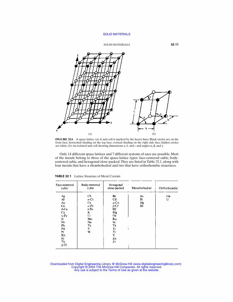
Only 14 different space lattices and 7 different systems of axes are possible. Mostof the metals belong to three of the space-lattice types: face-centered cubic, body-centered cubic, and hexagonal close-packed.They are listed in Table 32.1, along withfour metals that have a rhombohedral and two that have orthorhombic structures.
SOLID MATERIALS 32.11
FIGURE 32.6 A space lattice. (a) A unit cell is marked by the heavy lines. Black circles are on thefront face; horizontal shading on the top face; vertical shading on the right side face; hidden circlesare white. (b) An isolated unit cell showing dimensions a, b, and c and angles α, β, and γ.
(a) (b)
TABLE 32.1 Lattice Structure of Metal Crystals
SOLID MATERIALS
Downloaded from Digital Engineering Library @ McGraw-Hill (www.digitalengineeringlibrary.com)Copyright © 2004 The McGraw-Hill Companies. All rights reserved.
Any use is subject to the Terms of Use as given at the website.
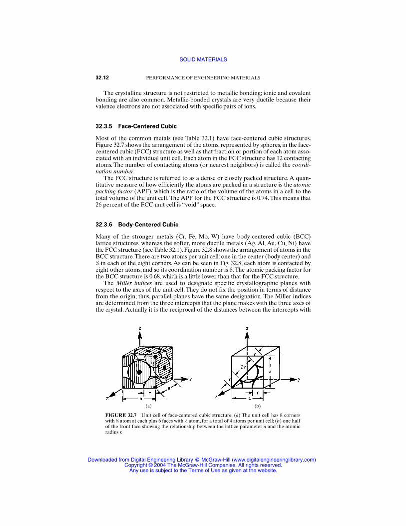
The crystalline structure is not restricted to metallic bonding; ionic and covalentbonding are also common. Metallic-bonded crystals are very ductile because theirvalence electrons are not associated with specific pairs of ions.
32.3.5 Face-Centered Cubic
Most of the common metals (see Table 32.1) have face-centered cubic structures.Figure 32.7 shows the arrangement of the atoms, represented by spheres, in the face-centered cubic (FCC) structure as well as that fraction or portion of each atom asso-ciated with an individual unit cell. Each atom in the FCC structure has 12 contactingatoms. The number of contacting atoms (or nearest neighbors) is called the coordi-nation number.
The FCC structure is referred to as a dense or closely packed structure. A quan-titative measure of how efficiently the atoms are packed in a structure is the atomicpacking factor (APF), which is the ratio of the volume of the atoms in a cell to thetotal volume of the unit cell. The APF for the FCC structure is 0.74. This means that26 percent of the FCC unit cell is “void” space.
32.3.6 Body-Centered Cubic
Many of the stronger metals (Cr, Fe, Mo, W) have body-centered cubic (BCC) lattice structures, whereas the softer, more ductile metals (Ag, Al, Au, Cu, Ni) havethe FCC structure (see Table 32.1). Figure 32.8 shows the arrangement of atoms in theBCC structure.There are two atoms per unit cell: one in the center (body center) and1⁄8 in each of the eight corners. As can be seen in Fig. 32.8, each atom is contacted byeight other atoms, and so its coordination number is 8. The atomic packing factor forthe BCC structure is 0.68, which is a little lower than that for the FCC structure.
The Miller indices are used to designate specific crystallographic planes withrespect to the axes of the unit cell. They do not fix the position in terms of distancefrom the origin; thus, parallel planes have the same designation. The Miller indicesare determined from the three intercepts that the plane makes with the three axes ofthe crystal. Actually it is the reciprocal of the distances between the intercepts with
32.12 PERFORMANCE OF ENGINEERING MATERIALS
FIGURE 32.7 Unit cell of face-centered cubic structure. (a) The unit cell has 8 cornerswith 1⁄8 atom at each plus 6 faces with 1⁄2 atom, for a total of 4 atoms per unit cell; (b) one halfof the front face showing the relationship between the lattice parameter a and the atomicradius r.
(a) (b)
SOLID MATERIALS
Downloaded from Digital Engineering Library @ McGraw-Hill (www.digitalengineeringlibrary.com)Copyright © 2004 The McGraw-Hill Companies. All rights reserved.
Any use is subject to the Terms of Use as given at the website.
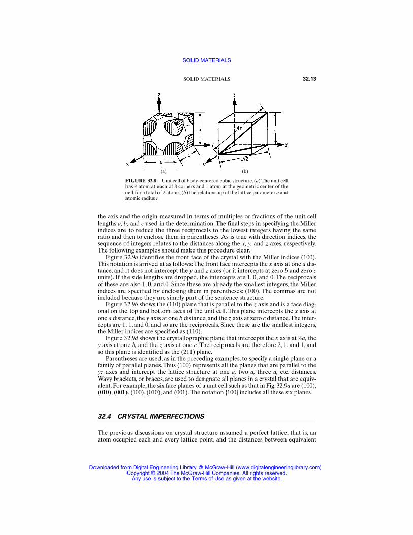
the axis and the origin measured in terms of multiples or fractions of the unit celllengths a, b, and c used in the determination. The final steps in specifying the Millerindices are to reduce the three reciprocals to the lowest integers having the sameratio and then to enclose them in parentheses. As is true with direction indices, thesequence of integers relates to the distances along the x, y, and z axes, respectively.The following examples should make this procedure clear.
Figure 32.9a identifies the front face of the crystal with the Miller indices (100).This notation is arrived at as follows:The front face intercepts the x axis at one a dis-tance, and it does not intercept the y and z axes (or it intercepts at zero b and zero cunits). If the side lengths are dropped, the intercepts are 1, 0, and 0. The reciprocalsof these are also 1, 0, and 0. Since these are already the smallest integers, the Millerindices are specified by enclosing them in parentheses: (100). The commas are notincluded because they are simply part of the sentence structure.
Figure 32.9b shows the (110) plane that is parallel to the z axis and is a face diag-onal on the top and bottom faces of the unit cell. This plane intercepts the x axis atone a distance, the y axis at one b distance, and the z axis at zero c distance.The inter-cepts are 1, 1, and 0, and so are the reciprocals. Since these are the smallest integers,the Miller indices are specified as (110).
Figure 32.9d shows the crystallographic plane that intercepts the x axis at 1⁄2a, they axis at one b, and the z axis at one c. The reciprocals are therefore 2, 1, and 1, andso this plane is identified as the (211) plane.
Parentheses are used, as in the preceding examples, to specify a single plane or afamily of parallel planes. Thus (100) represents all the planes that are parallel to theyz axes and intercept the lattice structure at one a, two a, three a, etc. distances.Wavy brackets, or braces, are used to designate all planes in a crystal that are equiv-alent. For example, the six face planes of a unit cell such as that in Fig. 32.9a are (100),(010), (001), (100), (010), and (001). The notation 100 includes all these six planes.
32.4 CRYSTAL IMPERFECTIONS
The previous discussions on crystal structure assumed a perfect lattice; that is, anatom occupied each and every lattice point, and the distances between equivalent
SOLID MATERIALS 32.13
FIGURE 32.8 Unit cell of body-centered cubic structure. (a) The unit cellhas 1⁄8 atom at each of 8 corners and 1 atom at the geometric center of thecell, for a total of 2 atoms; (b) the relationship of the lattice parameter a andatomic radius r.
(a) (b)
SOLID MATERIALS
Downloaded from Digital Engineering Library @ McGraw-Hill (www.digitalengineeringlibrary.com)Copyright © 2004 The McGraw-Hill Companies. All rights reserved.
Any use is subject to the Terms of Use as given at the website.
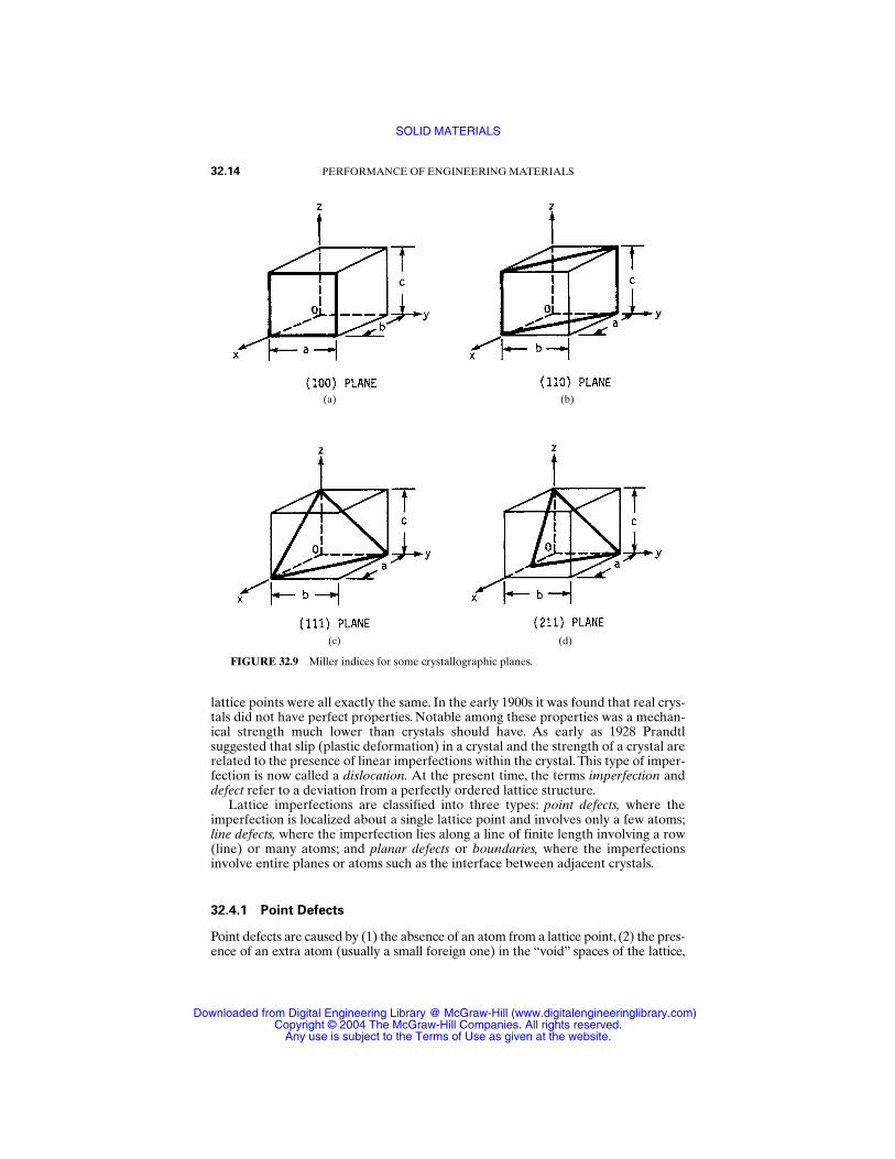
lattice points were all exactly the same. In the early 1900s it was found that real crys-tals did not have perfect properties. Notable among these properties was a mechan-ical strength much lower than crystals should have. As early as 1928 Prandtlsuggested that slip (plastic deformation) in a crystal and the strength of a crystal arerelated to the presence of linear imperfections within the crystal.This type of imper-fection is now called a dislocation. At the present time, the terms imperfection anddefect refer to a deviation from a perfectly ordered lattice structure.
Lattice imperfections are classified into three types: point defects, where theimperfection is localized about a single lattice point and involves only a few atoms;line defects, where the imperfection lies along a line of finite length involving a row(line) or many atoms; and planar defects or boundaries, where the imperfectionsinvolve entire planes or atoms such as the interface between adjacent crystals.
32.4.1 Point Defects
Point defects are caused by (1) the absence of an atom from a lattice point, (2) the pres-ence of an extra atom (usually a small foreign one) in the “void” spaces of the lattice,
32.14 PERFORMANCE OF ENGINEERING MATERIALS
FIGURE 32.9 Miller indices for some crystallographic planes.
(a)
(c)
(b)
(d)
SOLID MATERIALS
Downloaded from Digital Engineering Library @ McGraw-Hill (www.digitalengineeringlibrary.com)Copyright © 2004 The McGraw-Hill Companies. All rights reserved.
Any use is subject to the Terms of Use as given at the website.
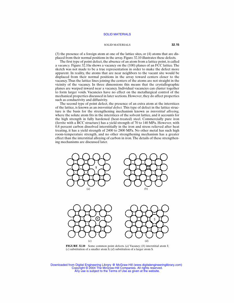
(3) the presence of a foreign atom at one of the lattice sites, or (4) atoms that are dis-placed from their normal positions in the array. Figure 32.10 illustrates these defects.
The first type of point defect, the absence of an atom from a lattice point, is calleda vacancy. Figure 32.10a shows a vacancy on the (100) planes of an FCC lattice. Thesketch was not made to be a true representation in order to make the defect moreapparent. In reality, the atoms that are near neighbors to the vacant site would bedisplaced from their normal positions in the array toward centers closer to thevacancy. Thus the lattice lines joining the centers of the atoms are not straight in thevicinity of the vacancy. In three dimensions this means that the crystallographicplanes are warped inward near a vacancy. Individual vacancies can cluster togetherto form larger voids. Vacancies have no effect on the metallurgical control of themechanical properties discussed in later sections. However, they do affect propertiessuch as conductivity and diffusivity.
The second type of point defect, the presence of an extra atom at the intersticesof the lattice, is known as an interstitial defect. This type of defect in the lattice struc-ture is the basis for the strengthening mechanism known as interstitial alloying,where the solute atom fits in the interstices of the solvent lattice, and it accounts forthe high strength in fully hardened (heat-treated) steel. Commercially pure iron(ferrite with a BCC structure) has a yield strength of 70 to 140 MPa. However, with0.8 percent carbon dissolved interstitially in the iron and stress relieved after heattreating, it has a yield strength of 2400 to 2800 MPa. No other metal has such highroom-temperature strength, and no other strengthening mechanism has a greatereffect than the interstitial alloying of carbon in iron. The details of these strengthen-ing mechanisms are discussed later.
SOLID MATERIALS 32.15
FIGURE 32.10 Some common point defects. (a) Vacancy; (b) interstitial atom I;(c) substitution of a smaller atom S; (d) substitution of a larger atom S.
(a) (b)
(c) (d)
SOLID MATERIALS
Downloaded from Digital Engineering Library @ McGraw-Hill (www.digitalengineeringlibrary.com)Copyright © 2004 The McGraw-Hill Companies. All rights reserved.
Any use is subject to the Terms of Use as given at the website.
Figure 32.10b shows an interstitial atom I in the solvent matrix. However, it doesnot lie in the plane of the solvent lattice but lies either above or below the sketchedplane. Also, the foreign atom is always larger than the “void” space it occupies, andso it necessarily forces the surrounding solvent atoms out of their normal array.Therefore, the crystallographic planes are warped outward in the vicinity of an inter-stitial defect.
The third type of point defect, the presence of a foreign atom at one of the latticepoints, is referred to as a substitutional defect. When an alloy is made by addingsolute atoms that replace (substitute for) solvent atoms in the lattice structure, it iscalled a substitutional alloy. This type is the most common one in the metal system.Figure 32.10c and d shows the substitution of a smaller and a larger atom S at one ofthe lattice points. Unlike the interstitial atom, the substitutional one is in the planeof the solvent matrix. The crystallographic planes are also warped in the vicinity ofthe substitutional defect, inward for the smaller atom and outward for the largeratom. The distortion of the crystallographic planes is very important to an under-standing of control of the strength of materials, which is presented later.
The fourth type of point defect, atoms that are displaced from their normal posi-tion, occurs in several forms. The atoms in the “contacting” planes of two adjoiningcrystals are not in their normal positions as a result of the crystals having solidifiedfrom the liquid without being in perfect registry with each other. This is consideredto be a grain boundary defect, which has a significant effect on the strength of allpolycrystalline materials.
Two additional types of atom displacement defects occur in ionic crystals that arenot present in metallic-bonded crystals. A vacancy in an ionic crystal that is associ-ated with a displaced pair, one cation and one anion, is called a Schottky defect. AFrenkel defect occurs when a small cation moves from a lattice point, leaving avacancy, and occupies an interstitial site.
32.4.2 Line Defects or Dislocations
Examinations of crystals under the electron microscope have shown interruptions inthe periodicity of the lattice structure in certain directions. In a two-dimensional rep-resentation these interruptions appear as lines; hence the name line defects. It isbelieved that a perfect crystal of a metal such as pure iron should have a strength of1 or 2 million pounds force per square inch, whereas in reality such perfect crystalshave a yield strength of only a few thousand. The reason given for the three ordersof magnitude difference between the postulated and actual strength of metal crys-tals is the presence of these line defects.
The two most common line defects are edge dislocation and screw dislocation.An edge dislocation is the line defect that results from the presence of an extra planeof atoms in one portion of a crystal compared to the adjacent part. Actually, it is theedge of this extra plane of atoms and runs from one end of the crystal to the other.When looking at the crystalline plane that is perpendicular to the dislocation line,the imperfection appears as an extra row of atoms in a part of the crystal.
An edge dislocation is customarily represented by a symbol in which the verticalleg designates the extra plane of atoms. When the vertical leg is above the horizon-tal leg, the dislocation is considered positive.When the extra plane of atoms is in thebottom portion of the crystal, the vertical leg is placed below the horizontal one andthe dislocation is said to be negative. The part of the crystal containing the extraplane of atoms is in compression, whereas that portion on the other side of the dis-location line is in tension. Since one dislocation line runs completely across a crystal,it deforms the lattice structure to a greater extent than does one point defect.
32.16 PERFORMANCE OF ENGINEERING MATERIALS
SOLID MATERIALS
Downloaded from Digital Engineering Library @ McGraw-Hill (www.digitalengineeringlibrary.com)Copyright © 2004 The McGraw-Hill Companies. All rights reserved.
Any use is subject to the Terms of Use as given at the website.
A screw dislocation is a crystal defect in which the lattice points lie on a spiral orhelical surface that revolves around a center line that is called the dislocation line. Ascrew dislocation terminates at a crystal surface. Shear stresses are set up in the lat-tice surrounding a screw dislocation as a result of the distortion in atomic array thatthe defect causes.
The Burgers vector is the distance, measured in multiples of the lattice parameter,that is needed to close a straight-sided loop around a dislocation when going thesame number of lattice distances in all four directions. It is the term used to definethe size of a dislocation and is designated by the letter b. A characteristic of an edgedislocation is that it lies perpendicular to its Burgers vector, whereas a screw dislo-cation lies parallel to its Burgers vector.
32.4.3 Planar Defects
There are several types of planar (or surface) defects that occur from a change in theorientation of crystallographic planes across a surface boundary. The most impor-tant planar defect is the grain boundary, which is the imperfect plane surface thatseparates two crystals of different orientation in a polycrystalline solid. Grainboundaries originate when the last few remaining atoms of a liquid freeze onto themeeting faces of two adjacent crystals that have grown from the melt or, similarly,when two adjacent crystals that grow by recrystallization meet each other.
The material in the grain boundary is at a higher energy level than the materialnear the center of the grain because of the increased elastic strain energy of theatoms that are forced from their normal (lowest-energy) sites in a perfect lattice.This higher energy level and lattice distortion cause the grain boundary material tobe stronger, have a higher diffusion rate, and serve as a more favorable site for thenucleation of second phases than the interior materials.
Another important planar defect is the twin boundary, which is the plane thatseparates two portions of a single crystal having slightly different orientations. Thetwo twins are mirror images of each other. The distortion of the twinned lattice islow in comparison to that at a grain boundary. Twins which form in most FCC metalcrystals, especially the copper- and nickel-base alloys, during freezing from the meltor recrystallization are called annealing twins. Twins which form in some metals dur-ing cold work (plastic deformation) are called mechanical twins.
A third planar defect is the low-angle grain boundary or low-angle tilt boundary,where the angular misalignment of the two grains is very small, on the order of a fewdegrees. In a sense it is a very undistorted grain boundary. The angular mismatch ofthe crystal planes is due to a row of dislocations piled above each other.
A stacking fault is a planar defect that occurs when one crystalline plane isstacked out of its normal sequence in the lattice array.The lattice on both sides of thedefect is normal. For example, the normal FCC stacking of planes may be inter-rupted by one layer of a hexagonal close-packed (HCP) plane, since both are close-packed structures with atomic packing factors of 0.74. Such stacking faults can occurduring the formation of a crystal or by plastic deformation.
32.5 SLIP IN CRYSTALLINE SOLIDS
Slip can be defined as the massive sliding movement of one large body of atoms withrespect to the remaining body of atoms of the crystal along crystallographic planes.Slip can also be considered as an avalanche of dislocations along one plane that pile
SOLID MATERIALS 32.17
SOLID MATERIALS
Downloaded from Digital Engineering Library @ McGraw-Hill (www.digitalengineeringlibrary.com)Copyright © 2004 The McGraw-Hill Companies. All rights reserved.
Any use is subject to the Terms of Use as given at the website.
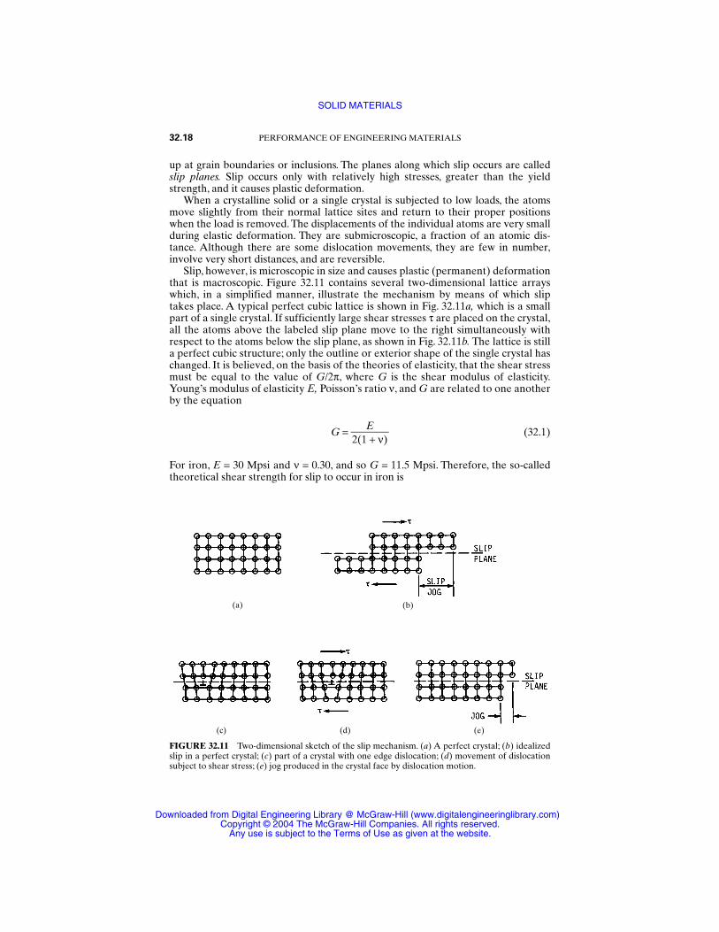
up at grain boundaries or inclusions. The planes along which slip occurs are calledslip planes. Slip occurs only with relatively high stresses, greater than the yieldstrength, and it causes plastic deformation.
When a crystalline solid or a single crystal is subjected to low loads, the atomsmove slightly from their normal lattice sites and return to their proper positionswhen the load is removed. The displacements of the individual atoms are very smallduring elastic deformation. They are submicroscopic, a fraction of an atomic dis-tance. Although there are some dislocation movements, they are few in number,involve very short distances, and are reversible.
Slip, however, is microscopic in size and causes plastic (permanent) deformationthat is macroscopic. Figure 32.11 contains several two-dimensional lattice arrayswhich, in a simplified manner, illustrate the mechanism by means of which sliptakes place. A typical perfect cubic lattice is shown in Fig. 32.11a, which is a smallpart of a single crystal. If sufficiently large shear stresses τ are placed on the crystal,all the atoms above the labeled slip plane move to the right simultaneously withrespect to the atoms below the slip plane, as shown in Fig. 32.11b. The lattice is stilla perfect cubic structure; only the outline or exterior shape of the single crystal haschanged. It is believed, on the basis of the theories of elasticity, that the shear stressmust be equal to the value of G/2π, where G is the shear modulus of elasticity.Young’s modulus of elasticity E, Poisson’s ratio ν, and G are related to one anotherby the equation
G = 2(1
E+ ν) (32.1)
For iron, E = 30 Mpsi and ν = 0.30, and so G = 11.5 Mpsi. Therefore, the so-calledtheoretical shear strength for slip to occur in iron is
32.18 PERFORMANCE OF ENGINEERING MATERIALS
FIGURE 32.11 Two-dimensional sketch of the slip mechanism. (a) A perfect crystal; (b) idealizedslip in a perfect crystal; (c) part of a crystal with one edge dislocation; (d) movement of dislocationsubject to shear stress; (e) jog produced in the crystal face by dislocation motion.
(a) (b)
(c) (d) (e)
SOLID MATERIALS
Downloaded from Digital Engineering Library @ McGraw-Hill (www.digitalengineeringlibrary.com)Copyright © 2004 The McGraw-Hill Companies. All rights reserved.
Any use is subject to the Terms of Use as given at the website.
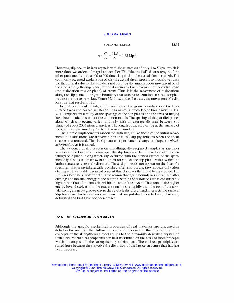
τ = 2Gπ =
121π.5 = 1.83 Mpsi
However, slip occurs in iron crystals with shear stresses of only 4 to 5 kpsi, which ismore than two orders of magnitude smaller. The “theoretical” shear strength of theother pure metals is also 400 to 500 times larger than the actual shear strength. Thecommonly accepted explanation of why the actual shear stress is so much lower thanthe theoretical value is that slip does not occur by the simultaneous movement of allthe atoms along the slip plane; rather, it occurs by the movement of individual rows(the dislocation row or plane) of atoms. Thus it is the movement of dislocationsalong the slip plane to the grain boundary that causes the actual shear stress for plas-tic deformation to be so low. Figure 32.11c, d, and e illustrates the movement of a dis-location that results in slip.
In real crystals of metals, slip terminates at the grain boundaries or the free-surface faces and causes substantial jogs or steps, much larger than shown in Fig.32.11. Experimental study of the spacings of the slip planes and the sizes of the joghave been made on some of the common metals. The spacing of the parallel planesalong which slip occurs varies randomly, with an average distance between slipplanes of about 2000 atom diameters. The length of the step or jog at the surface ofthe grain is approximately 200 to 700 atom diameters.
The atomic displacements associated with slip, unlike those of the initial move-ments of dislocations, are irreversible in that the slip jog remains when the shearstresses are removed. That is, slip causes a permanent change in shape, or plasticdeformation, as it is called.
The evidence of slip is seen on metallurgically prepared samples as slip lineswhen examined under a microscope. The slip lines are the intersection of the crys-tallographic planes along which slip occurred with the etched surface of the speci-men. Slip results in a narrow band on either side of the slip plane within which thelattice structure is severely distorted. These slip lines do not appear on the face of aspecimen that is metallurgically polished after slip occurs; they appear only afteretching with a suitable chemical reagent that dissolves the metal being studied. Theslip lines become visible for the same reason that grain boundaries are visible afteretching:The internal energy of the material within the distorted area is considerablyhigher than that of the material within the rest of the crystal.The metal in the higherenergy level dissolves into the reagent much more rapidly than the rest of the crys-tal, leaving a narrow groove where the severely distorted band intersects the surface.Slip lines can also be seen on specimens that are polished prior to being plasticallydeformed and that have not been etched.
32.6 MECHANICAL STRENGTH
Although the specific mechanical properties of real materials are discussed indetail in the material that follows, it is very appropriate at this time to relate theconcepts of the strengthening mechanisms to the previously described crystallinestructures. Mechanical properties can best be studied on the basis of three preceptswhich encompass all the strengthening mechanisms. These three principles arestated here because they involve the distortion of the lattice structure that has justbeen discussed.
SOLID MATERIALS 32.19
SOLID MATERIALS
Downloaded from Digital Engineering Library @ McGraw-Hill (www.digitalengineeringlibrary.com)Copyright © 2004 The McGraw-Hill Companies. All rights reserved.
Any use is subject to the Terms of Use as given at the website.
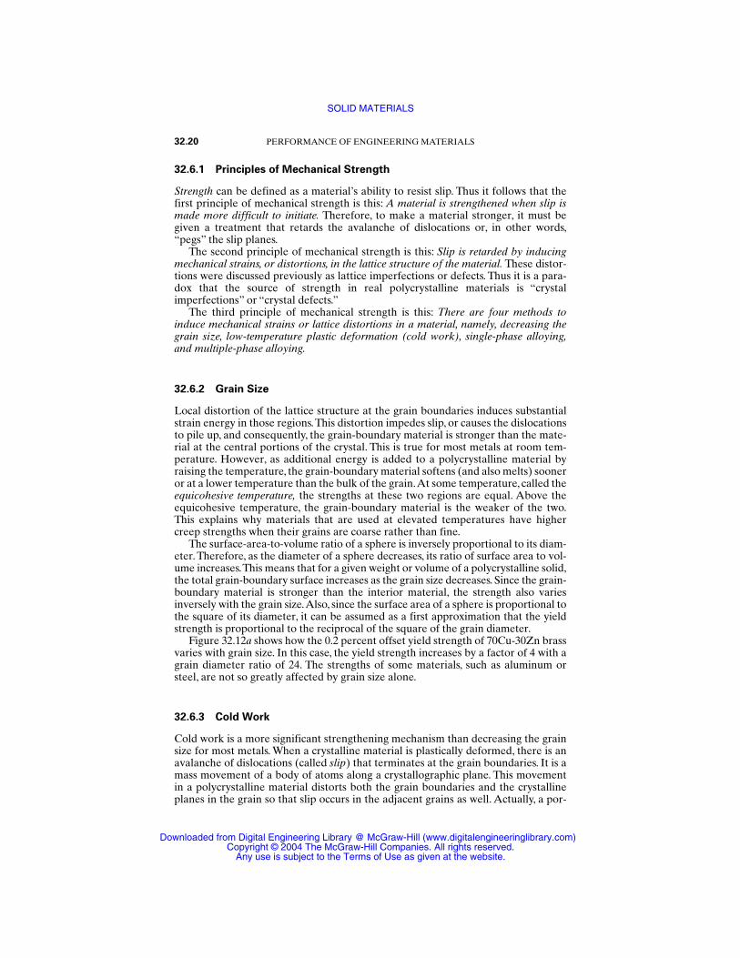
32.6.1 Principles of Mechanical Strength
Strength can be defined as a material’s ability to resist slip. Thus it follows that thefirst principle of mechanical strength is this: A material is strengthened when slip ismade more difficult to initiate. Therefore, to make a material stronger, it must begiven a treatment that retards the avalanche of dislocations or, in other words,“pegs” the slip planes.
The second principle of mechanical strength is this: Slip is retarded by inducingmechanical strains, or distortions, in the lattice structure of the material. These distor-tions were discussed previously as lattice imperfections or defects. Thus it is a para-dox that the source of strength in real polycrystalline materials is “crystalimperfections” or “crystal defects.”
The third principle of mechanical strength is this: There are four methods toinduce mechanical strains or lattice distortions in a material, namely, decreasing thegrain size, low-temperature plastic deformation (cold work), single-phase alloying,and multiple-phase alloying.
32.6.2 Grain Size
Local distortion of the lattice structure at the grain boundaries induces substantialstrain energy in those regions.This distortion impedes slip, or causes the dislocationsto pile up, and consequently, the grain-boundary material is stronger than the mate-rial at the central portions of the crystal. This is true for most metals at room tem-perature. However, as additional energy is added to a polycrystalline material byraising the temperature, the grain-boundary material softens (and also melts) sooneror at a lower temperature than the bulk of the grain.At some temperature, called theequicohesive temperature, the strengths at these two regions are equal. Above theequicohesive temperature, the grain-boundary material is the weaker of the two.This explains why materials that are used at elevated temperatures have highercreep strengths when their grains are coarse rather than fine.
The surface-area-to-volume ratio of a sphere is inversely proportional to its diam-eter. Therefore, as the diameter of a sphere decreases, its ratio of surface area to vol-ume increases.This means that for a given weight or volume of a polycrystalline solid,the total grain-boundary surface increases as the grain size decreases. Since the grain-boundary material is stronger than the interior material, the strength also variesinversely with the grain size.Also, since the surface area of a sphere is proportional tothe square of its diameter, it can be assumed as a first approximation that the yieldstrength is proportional to the reciprocal of the square of the grain diameter.
Figure 32.12a shows how the 0.2 percent offset yield strength of 70Cu-30Zn brassvaries with grain size. In this case, the yield strength increases by a factor of 4 with agrain diameter ratio of 24. The strengths of some materials, such as aluminum orsteel, are not so greatly affected by grain size alone.
32.6.3 Cold Work
Cold work is a more significant strengthening mechanism than decreasing the grainsize for most metals. When a crystalline material is plastically deformed, there is anavalanche of dislocations (called slip) that terminates at the grain boundaries. It is amass movement of a body of atoms along a crystallographic plane. This movementin a polycrystalline material distorts both the grain boundaries and the crystallineplanes in the grain so that slip occurs in the adjacent grains as well. Actually, a por-
32.20 PERFORMANCE OF ENGINEERING MATERIALS
SOLID MATERIALS
Downloaded from Digital Engineering Library @ McGraw-Hill (www.digitalengineeringlibrary.com)Copyright © 2004 The McGraw-Hill Companies. All rights reserved.
Any use is subject to the Terms of Use as given at the website.
tion of one grain intrudes into the space that was previously occupied by anothergrain, with a resulting distortion of the lattice in both grains.
Figure 32.12b illustrates the effect of cold work on the yield strength of 70Cu-30Zn brass.With only 10 percent cold work, the yield strength is raised by a factor of3.5, and 60 percent cold work increases the strength nearly 8 times. In general, 10percent cold work more than doubles the yield strength of most metals.
32.6.4 Single-Phase Alloying
Alloying (single- and multiple-phase) is the most important of the methods avail-able to control or manipulate the mechanical properties of materials. The greatestincrease in strength known today occurs when iron having a yield strength of 10 to20 kpsi (70 to 140 MPa) is alloyed with less than 1.0 percent carbon to form a singlephase (martensite) that has a yield strength of nearly 435 kpsi (3000 MPa).
The lattice is distorted and dislocation movement is impeded when foreign(solute) atoms are added to the lattice structure of a pure material. Figure 32.10bthrough d illustrates this condition, which was discussed previously under the head-ing “Point Defects.” Vacancy defects, as shown in Fig. 32.10a, are not a practicalstrengthening method. The reason single-phase alloying has such a great effect onstrength is that the entire lattice network is distorted, and uniformly, whereas in theother mechanism, there are regions in each crystal that are severely distorted andother regions that are hardly distorted at all.
Figure 32.13a shows the effect on the strength of the material of adding a foreignelement B or C to the lattice structure of element A. From this figure it is clear thatnot all elements have the same strengthening effect. In general, the further the ratioof diameters of solute to solvent atoms is from unity, the greater will be the strength-ening effect. However, the further this ratio is from unity, as previously explained,the less soluble the two atoms are in each other’s lattice.
32.6.5 Multiple-Phase Alloying
This mechanism is sometimes referred to as fine-particle strengthening. In a sense,multiple-phase alloying is a combination of single-phase alloying and grain-boundary
SOLID MATERIALS 32.21
FIGURE 32.12 Yield strength versus grain size (a) and percent cold work (b) for 70Cu-30Znbrass.
(a) (b)
SOLID MATERIALS
Downloaded from Digital Engineering Library @ McGraw-Hill (www.digitalengineeringlibrary.com)Copyright © 2004 The McGraw-Hill Companies. All rights reserved.
Any use is subject to the Terms of Use as given at the website.
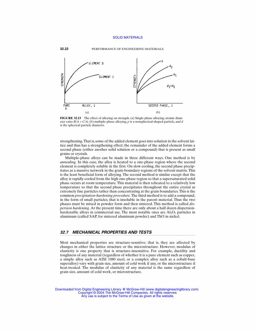
strengthening.That is, some of the added element goes into solution in the solvent lat-tice and thus has a strengthening effect; the remainder of the added element forms asecond phase (either another solid solution or a compound) that is present as smallgrains or crystals.
Multiple-phase alloys can be made in three different ways. One method is byannealing. In this case, the alloy is heated to a one-phase region where the secondelement is completely soluble in the first. On slow cooling, the second phase precip-itates as a massive network in the grain-boundary regions of the solvent matrix.Thisis the least beneficial form of alloying. The second method is similar except that thealloy is rapidly cooled from the high one-phase region so that a supersaturated solidphase occurs at room temperature. This material is then reheated to a relatively lowtemperature so that the second phase precipitates throughout the entire crystal asextremely fine particles rather than concentrating at the grain boundaries.This is thecommon precipitation-hardening procedure. The third method is to add a compound,in the form of small particles, that is insoluble in the parent material. Thus the twophases must be mixed in powder form and then sintered. This method is called dis-persion hardening. At the present time there are only about a half dozen dispersion-hardenable alloys in commercial use. The most notable ones are Al2O3 particles inaluminum (called SAP, for sintered aluminum powder) and ThO in nickel.
32.7 MECHANICAL PROPERTIES AND TESTS
Most mechanical properties are structure-sensitive; that is, they are affected bychanges in either the lattice structure or the microstructure. However, modulus ofelasticity is one property that is structure-insensitive. For example, ductility andtoughness of any material (regardless of whether it is a pure element such as copper,a simple alloy such as AISI 1080 steel, or a complex alloy such as a cobalt-basesuperalloy) vary with grain size, amount of cold work if any, or the microstructure ifheat-treated. The modulus of elasticity of any material is the same regardless ofgrain size, amount of cold work, or microstructure.
32.22 PERFORMANCE OF ENGINEERING MATERIALS
FIGURE 32.13 The effect of alloying on strength. (a) Single-phase alloying; atomic diam-eter ratio B/A > C/A; (b) multiple-phase alloying; p is a nonspherical-shaped particle, and dis the spherical particle diameter.
(a) (b)
SOLID MATERIALS
Downloaded from Digital Engineering Library @ McGraw-Hill (www.digitalengineeringlibrary.com)Copyright © 2004 The McGraw-Hill Companies. All rights reserved.
Any use is subject to the Terms of Use as given at the website.
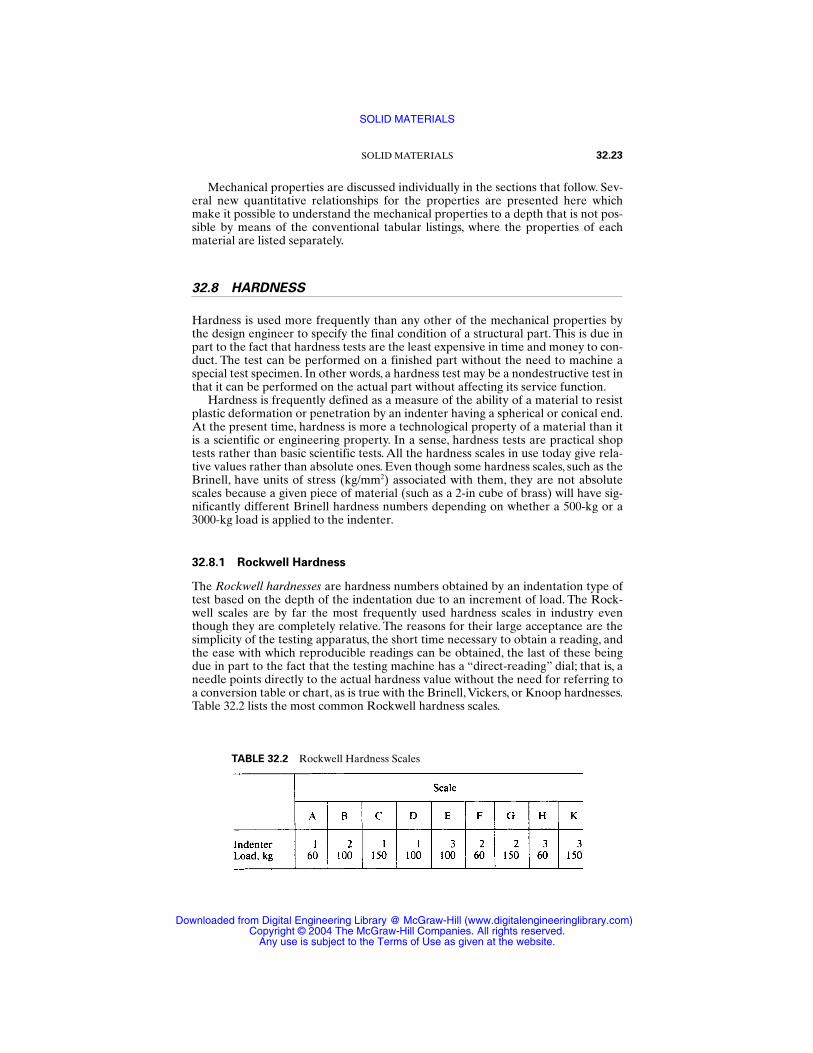
Mechanical properties are discussed individually in the sections that follow. Sev-eral new quantitative relationships for the properties are presented here whichmake it possible to understand the mechanical properties to a depth that is not pos-sible by means of the conventional tabular listings, where the properties of eachmaterial are listed separately.
32.8 HARDNESS
Hardness is used more frequently than any other of the mechanical properties bythe design engineer to specify the final condition of a structural part. This is due inpart to the fact that hardness tests are the least expensive in time and money to con-duct. The test can be performed on a finished part without the need to machine aspecial test specimen. In other words, a hardness test may be a nondestructive test inthat it can be performed on the actual part without affecting its service function.
Hardness is frequently defined as a measure of the ability of a material to resistplastic deformation or penetration by an indenter having a spherical or conical end.At the present time, hardness is more a technological property of a material than itis a scientific or engineering property. In a sense, hardness tests are practical shoptests rather than basic scientific tests. All the hardness scales in use today give rela-tive values rather than absolute ones. Even though some hardness scales, such as theBrinell, have units of stress (kg/mm2) associated with them, they are not absolutescales because a given piece of material (such as a 2-in cube of brass) will have sig-nificantly different Brinell hardness numbers depending on whether a 500-kg or a3000-kg load is applied to the indenter.
32.8.1 Rockwell Hardness
The Rockwell hardnesses are hardness numbers obtained by an indentation type oftest based on the depth of the indentation due to an increment of load. The Rock-well scales are by far the most frequently used hardness scales in industry eventhough they are completely relative. The reasons for their large acceptance are thesimplicity of the testing apparatus, the short time necessary to obtain a reading, andthe ease with which reproducible readings can be obtained, the last of these beingdue in part to the fact that the testing machine has a “direct-reading” dial; that is, aneedle points directly to the actual hardness value without the need for referring toa conversion table or chart, as is true with the Brinell,Vickers, or Knoop hardnesses.Table 32.2 lists the most common Rockwell hardness scales.
SOLID MATERIALS 32.23
TABLE 32.2 Rockwell Hardness Scales
SOLID MATERIALS
Downloaded from Digital Engineering Library @ McGraw-Hill (www.digitalengineeringlibrary.com)Copyright © 2004 The McGraw-Hill Companies. All rights reserved.
Any use is subject to the Terms of Use as given at the website.
Indenter 1 is a diamond cone having an included angle of 120° and a sphericalend radius of 0.008 in. Indenters 2 and 3 are 1⁄16-in-diameter and 1⁄8-in-diameter balls,respectively. In addition to the preceding scales, there are several others for testingvery soft bearing materials, such as babbit, that use 1⁄4-in-diameter and 1⁄2-in-diameterballs.Also, there are several “superficial” scales that use a special diamond cone withloads less than 50 kg to test the hardness of surface-hardened layers.
The particular materials that each scale is used on are as follows: the A scale onthe extremely hard materials, such as carbides or thin case-hardened layers on steel;the B scale on soft steels, copper and aluminum alloys, and soft-case irons; the Cscale on medium and hard steels, hard-case irons, and all hard nonferrous alloys; theE and F scales on soft copper and aluminum alloys.The remaining scales are used oneven softer alloys.
Several precautions must be observed in the proper use of the Rockwell scales.The ball indenter should not be used on any material having a hardness greater than50 RC; otherwise the steel ball will be plastically deformed or flattened and thus giveerroneous readings. Readings taken on the sides of cylinders or spheres should becorrected for the curvature of the surface. Readings on the C scale of less than 20should not be recorded or specified because they are unreliable and subject to muchvariation.
The hardness numbers for all the Rockwell scales are an inverse measure of thedepth of the indentation. Each division on the dial gauge of the Rockwell machinecorresponds to an 80 × 106 in depth of penetration. The penetration with the C scalevaries between 0.0005 in for hard steel and 0.0015 in for very soft steel when only theminor load is applied.The total depth of penetration with both the major and minorloads applied varies from 0.003 in for the hardest steel to 0.008 in for soft steel (20RC). Since these indentations are relatively shallow, the Rockwell C hardness test isconsidered a nondestructive test and it can be used on fairly thin parts.
Although negative hardness readings can be obtained on the Rockwell scales(akin to negative Fahrenheit temperature readings), they are usually not recorded assuch, but rather a different scale is used that gives readings greater than zero. Theonly exception to this is when one wants to show a continuous trend in the change inhardness of a material due to some treatment. A good example of this is the case ofthe effect of cold work on the hardness of a fully annealed brass. Here the annealedhardness may be −20 RB and increase to 95 RB with severe cold work.
32.8.2 Brinell Hardness
The Brinell hardness HB is the hardness number obtained by dividing the load thatis applied to a spherical indenter by the surface area of the spherical indentationproduced; it has units of kilograms per square millimeter. Most readings are takenwith a 10-mm ball of either hardened steel or tungsten carbide. The loads that areapplied vary from 500 kg for soft materials to 3000 kg for hard materials. The steelball should not be used on materials having a hardness greater than about 525 HB
(52 RC) because of the possibility of putting a flat spot on the ball and making it inac-curate for further use.
The Brinell hardness machine is as simple as, though more massive than, theRockwell hardness machine, but the standard model is not direct-reading and takesa longer time to obtain a reading than the Rockwell machine. In addition, the inden-tation is much larger than that produced by the Rockwell machine, and the machinecannot be used on hard steel. The method of operation, however, is simple. The pre-scribed load is applied to the 10-mm-diameter ball for approximately 10 s. The part
32.24 PERFORMANCE OF ENGINEERING MATERIALS
SOLID MATERIALS
Downloaded from Digital Engineering Library @ McGraw-Hill (www.digitalengineeringlibrary.com)Copyright © 2004 The McGraw-Hill Companies. All rights reserved.
Any use is subject to the Terms of Use as given at the website.
is then withdrawn from the machine and the operator measures the diameter of theindentation by means of a millimeter scale etched on the eyepiece of a specialBrinell microscope.The Brinell hardness number is then obtained from the equation
HB = (32.2)
where L = load, kgD = diameter of indenter, mmd = diameter of indentation, mm
The denominator in this equation is the spherical area of the indentation.The Brinell hardness test has proved to be very successful, partly due to the fact
that for some materials it can be directly correlated to the tensile strength. For exam-ple, the tensile strengths of all the steels, if stress-relieved, are very close to being 0.5times the Brinell hardness number when expressed in kilopounds per square inch(kpsi).This is true for both annealed and heat-treated steel. Even though the Brinellhardness test is a technological one, it can be used with considerable success in engi-neering research on the mechanical properties of materials and is a much better testfor this purpose than the Rockwell test.
The Brinell hardness number of a given material increases as the applied load isincreased, the increase being somewhat proportional to the strain-hardening rate ofthe material.This is due to the fact that the material beneath the indentation is plas-tically deformed, and the greater the penetration, the greater is the amount of coldwork, with a resulting high hardness. For example, the cobalt base alloy HS-25 has ahardness of 150 HB with a 500-kg load and a hardness of 201 HB with an applied loadof 3000 kg.
32.8.3 Meyer Hardness
The Meyer hardness HM is the hardness number obtained by dividing the loadapplied to a spherical indenter by the projected area of the indentation. The Meyerhardness test itself is identical to the Brinell test and is usually performed on aBrinell hardness-testing machine. The difference between these two hardness scalesis simply the area that is divided into the applied load—the projected area being usedfor the Meyer hardness and the spherical surface area for the Brinell hardness. Bothare based on the diameter of the indentation. The units of the Meyer hardness arealso kilograms per square millimeter, and hardness is calculated from the equation
HM = (32.3)
Because the Meyer hardness is determined from the projected area rather thanthe contact area, it is a more valid concept of stress and therefore is considered amore basic or scientific hardness scale.Although this is true, it has been used very lit-tle since it was first proposed in 1908, and then only in research studies. Its lack ofacceptance is probably due to the fact that it does not directly relate to the tensilestrength the way the Brinell hardness does.
Meyer is much better known for the original strain-hardening equation thatbears his name than he is for the hardness scale that bears his name. The strain-hardening equation for a given diameter of ball is
4Lπd 2
L(πD/2)[D − (D2 − d 2)1/2]
SOLID MATERIALS 32.25
SOLID MATERIALS
Downloaded from Digital Engineering Library @ McGraw-Hill (www.digitalengineeringlibrary.com)Copyright © 2004 The McGraw-Hill Companies. All rights reserved.
Any use is subject to the Terms of Use as given at the website.
L = Adp (32.4)
where L = load on spherical indenterd = diameter of indentationp = Meyer strain-hardening exponent
The values of the strain-hardening exponent for a variety of materials are availablein many handbooks.They vary from a minimum value of 2.0 for low-work-hardeningmaterials, such as the PH stainless steels and all cold-rolled metals, to a maximum ofabout 2.6 for dead soft brass.The value of p is about 2.25 for both annealed pure alu-minum and annealed 1020 steel.
Experimental data for some metals show that the exponent p in Eq. (32.4) isrelated to the strain-strengthening exponent m in the tensile stress-strain equation σ = σ0εm, which is to be presented later. The relation is
p − 2 = m (32.5)
In the case of 70-30 brass, which had an experimentally determined value of p = 2.53,a separately run tensile test gave a value of m = 0.53. However, such good agreementdoes not always occur, partly because of the difficulty of accurately measuring the diameter d. Nevertheless, this approximate relationship between the strain-hardening and the strain-strengthening exponents can be very useful in the practicalevaluation of the mechanical properties of a material.
32.8.4 Vickers or Diamond-Pyramid Hardness
The diamond-pyramid hardness Hp, or the Vickers hardness HV, as it is frequentlycalled, is the hardness number obtained by dividing the load applied to a square-based pyramid indenter by the surface area of the indentation. It is similar to theBrinell hardness test except for the indenter used.The indenter is made of industrialdiamond, and the area of the two pairs of opposite faces is accurately ground to anincluded angle of 136°. The load applied varies from as low as 100 g for microhard-ness readings to as high as 120 kg for the standard macrohardness readings. Theindentation at the surface of the workpiece is square-shaped. The diamond pyramidhardness number is determined by measuring the length of the two diagonals of theindentation and using the average value in the equation
Hp = = (32.6)
where L = applied load, kgd = diagonal of the indentation, mmα = face angle of the pyramid, 136°
The main advantage of a cone or pyramid indenter is that it produces indenta-tions that are geometrically similar regardless of depth. In order to be geometricallysimilar, the angle subtended by the indentation must be constant regardless of thedepth of the indentation. This is not true of a ball indenter. It is believed that if geo-metrically similar deformations are produced, the material being tested is stressed tothe same amount regardless of the depth of the penetration. On this basis, it wouldbe expected that conical or pyramidal indenters would give the same hardness num-
1.8544L
d 2
2L sin (α/2)
d 2
32.26 PERFORMANCE OF ENGINEERING MATERIALS
SOLID MATERIALS
Downloaded from Digital Engineering Library @ McGraw-Hill (www.digitalengineeringlibrary.com)Copyright © 2004 The McGraw-Hill Companies. All rights reserved.
Any use is subject to the Terms of Use as given at the website.
ber regardless of the load applied. Experimental data show that the pyramid hard-ness number is independent of the load if loads greater than 3 kg are applied. How-ever, for loads less than 3 kg, the hardness is affected by the load, depending on thestrain-hardening exponent of the material being tested.
32.8.5 Knoop Hardness
The Knoop hardness HK is the hardness number obtained by dividing the load appliedto a special rhombic-based pyramid indenter by the projected area of the indentation.The indenter is made of industrial diamond, and the four pyramid faces are ground sothat one of the angles between the intersections of the four faces is 172.5° and theother angle is 130°. A pyramid of this shape makes an indentation that has the pro-jected shape of a parallelogram having a long diagonal that is 7 times as large as theshort diagonal and 30 times as large as the maximum depth of the indentation.
The greatest application of Knoop hardness is in the microhardness area. Assuch, the indenter is mounted on an axis parallel to the barrel of a microscope hav-ing magnifications of 100× to 500×. A metallurgically polished flat specimen is used.The place at which the hardness is to be determined is located and positioned underthe hairlines of the microscope eyepiece. The specimen is then positioned under theindenter and the load is applied for 10 to 20 s.The specimen is then located under themicroscope again and the length of the long diagonal is measured. The Knoop hard-ness number is then determined by means of the equation
HK = (32.7)
where L = applied load, kgd = length of long diagonal, mm
The indenter constant 0.070 28 corresponds to the standard angles mentionedabove.
32.8.6 Scleroscope Hardness
The scleroscope hardness is the hardness number obtained from the height to which aspecial indenter bounces.The indenter has a rounded end and falls freely a distance of10 in in a glass tube. The rebound height is measured by visually observing the maxi-mum height the indenter reaches. The measuring scale is divided into 140 equal divi-sions and numbered beginning with zero. The scale was selected so that the reboundheight from a fully hardened high-carbon steel gives a maximum reading of 100.
All the previously described hardness scales are called static hardnesses becausethe load is slowly applied and maintained for several seconds.The scleroscope hard-ness, however, is a dynamic hardness. As such, it is greatly influenced by the elasticmodulus of the material being tested.
32.9 THE TENSILE TEST
The tensile test is conducted on a machine that can apply uniaxial tensile or com-pressive loads to the test specimen, and the machine also has provisions for accu-
L0.070 28d 2
SOLID MATERIALS 32.27
SOLID MATERIALS
Downloaded from Digital Engineering Library @ McGraw-Hill (www.digitalengineeringlibrary.com)Copyright © 2004 The McGraw-Hill Companies. All rights reserved.
Any use is subject to the Terms of Use as given at the website.
rately registering the value of the load and the amount of deformation that occurs tothe specimen. The tensile specimen may be a round cylinder or a flat strip with areduced cross section, called the gauge section, at its midlength to ensure that thefracture does not occur at the holding grips.The minimum length of the reduced sec-tion for a standard specimen is four times its diameter. The most commonly usedspecimen has a 0.505-in-diameter gauge section (0.2-in2 cross-sectional area) that is21⁄4 in long to accommodate a 2-in-long gauge section.The overall length of the spec-imen is 51⁄2 in, with a 1-in length of size 3⁄4-10NC screw threads on each end. TheASTM specifications list several other standard sizes, including flat specimens.
In addition to the tensile properties of strength, rigidity, and ductility, the tensiletest also gives information regarding the stress-strain behavior of the material. It isvery important to distinguish between strength and stress as they relate to materialproperties and mechanical design, but it is also somewhat awkward, since they havethe same units and many books use the same symbol for both.
Strength is a property of a material—it is a measure of the ability of a material towithstand stress or it is the load-carrying capacity of a material.The numerical valueof strength is determined by dividing the appropriate load (yield, maximum, frac-ture, shear, cyclic, creep, etc.) by the original cross-sectional area of the specimen andis designated as S. Thus
S = AL
0 (32.8)
The subscripts y, u, f, and s are appended to S to denote yield, ultimate, fracture, andshear strength, respectively. Although the strength values obtained from a tensiletest have the units of stress [psi (Pa) or equivalent], they are not really values ofstress.
Stress is a condition of a material due to an applied load. If there are no loads ona part, then there are no stresses in it. (Residual stresses may be considered as beingcaused by unseen loads.) The numerical value of the stress is determined by dividingthe actual load or force on the part by the actual cross section that is supporting theload. Normal stresses are almost universally designated by the symbol σ, and thestresses due to tensile loads are determined from the expression
σ = AL
i (32.9)
where Ai = instantaneous cross-sectional area corresponding to that particular load.The units of stress are pounds per square inch (pascals) or an equivalent.
During a tensile test, the stress varies from zero at the very beginning to a maxi-mum value that is equal to the true fracture stress, with an infinite number of stressesin between. However, the tensile test gives only three values of strength: yield, ulti-mate, and fracture. An appreciation of the real differences between strength andstress will be achieved after reading the material that follows on the use of tensile-test data.
32.9.1 Engineering Stress-Strain
Traditionally, the tensile test has been used to determine the so-called engineeringstress-strain data that are needed to plot the engineering stress-strain curve for agiven material. However, since engineering stress is not really a stress but is a mea-
32.28 PERFORMANCE OF ENGINEERING MATERIALS
SOLID MATERIALS
Downloaded from Digital Engineering Library @ McGraw-Hill (www.digitalengineeringlibrary.com)Copyright © 2004 The McGraw-Hill Companies. All rights reserved.
Any use is subject to the Terms of Use as given at the website.
sure of the strength of a material, it is more appropriate to call such data eitherstrength–nominal strain or nominal stress–strain data. Table 32.3 illustrates the datathat are normally collected during a tensile test, and Fig. 32.14 shows the conditionof a standard tensile specimen at the time the specific data in the table are recorded.The load-versus-gauge-length data, or an elastic stress-strain curve drawn by themachine, are needed to determine Young’s modulus of elasticity of the material aswell as the proportional limit. They are also needed to determine the yield strengthif the offset method is used. All the definitions associated with engineering stress-strain, or, more appropriately, with the strength–nominal strain properties, are pre-sented in the section which follows and are discussed in conjunction with theexperimental data for commercially pure titanium listed in Table 32.3 and Fig. 32.14.
The elastic and elastic-plastic data listed in Table 32.3 are plotted in Fig. 32.15with an expanded strain axis, which is necessary for the determination of the yieldstrength. The nominal (approximate) stress or the strength S which is calculated bymeans of Eq. (32.8) is plotted as the ordinate.
The abscissa of the engineering stress-strain plot is the nominal strain, which isdefined as the unit elongation obtained when the change in length is divided by theoriginal length and has the units of inch per inch and is designated as n. Thus, for ten-sion,
n = ∆
=
f
−0
0 (32.10)
where = gauge length and the subscripts 0 and f designate the original and finalstate, respectively. This equation is valid for deformation strains that do not exceedthe strain at the maximum load of a tensile specimen.
It is customary to plot the data obtained from a tensile test as a stress-strain curvesuch as that illustrated in Fig. 32.16, but without including the word nominal. Thereader then considers such a curve as an actual stress-strain curve, which it obviouslyis not. The curve plotted in Fig. 32.16 is in reality a load-deformation curve. If theordinate axis were labeled load (lb) rather than stress (psi), the distinction between
SOLID MATERIALS 32.29
TABLE 32.3 Tensile Test Data.
SOLID MATERIALS
Downloaded from Digital Engineering Library @ McGraw-Hill (www.digitalengineeringlibrary.com)Copyright © 2004 The McGraw-Hill Companies. All rights reserved.
Any use is subject to the Terms of Use as given at the website.
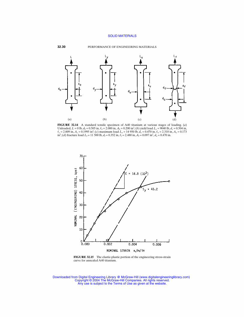
32.30 PERFORMANCE OF ENGINEERING MATERIALS
FIGURE 32.14 A standard tensile specimen of A40 titanium at various stages of loading. (a)Unloaded, L = 0 lb, d0 = 0.505 in, 0 = 2.000 in, A0 = 0.200 in2; (b) yield load Ly = 9040 lb, dy = 0.504 in,y = 2.009 in, Ay = 0.1995 in2; (c) maximum load Lu = 14 950 lb, du = 0.470 in, u = 2.310 in, Au = 0.173in2; (d) fracture load Lf = 11 500 lb, df = 0.352 in, f = 2.480 in, Af = 0.097 in2, du = 0.470 in.
(a) (b) (c) (d)
FIGURE 32.15 The elastic-plastic portion of the engineering stress-straincurve for annealed A40 titanium.
SOLID MATERIALS
Downloaded from Digital Engineering Library @ McGraw-Hill (www.digitalengineeringlibrary.com)Copyright © 2004 The McGraw-Hill Companies. All rights reserved.
Any use is subject to the Terms of Use as given at the website.
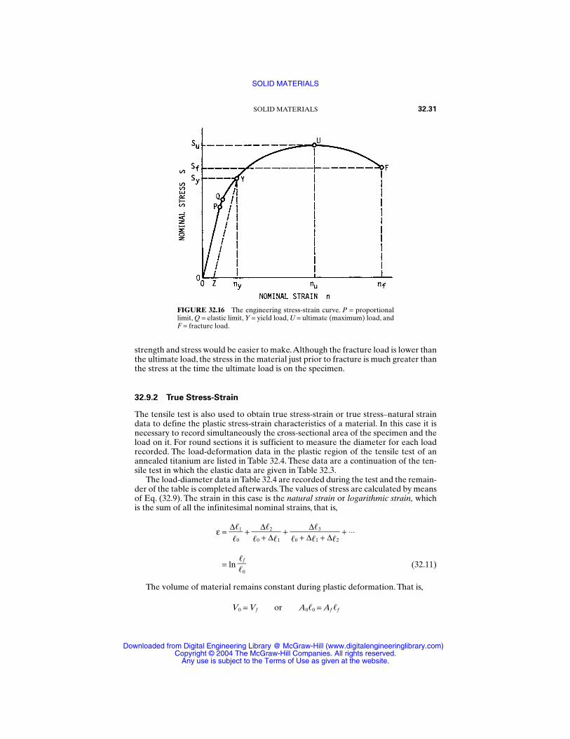
SOLID MATERIALS 32.31
FIGURE 32.16 The engineering stress-strain curve. P = proportionallimit, Q = elastic limit, Y = yield load, U = ultimate (maximum) load, andF = fracture load.
strength and stress would be easier to make.Although the fracture load is lower thanthe ultimate load, the stress in the material just prior to fracture is much greater thanthe stress at the time the ultimate load is on the specimen.
32.9.2 True Stress-Strain
The tensile test is also used to obtain true stress-strain or true stress–natural straindata to define the plastic stress-strain characteristics of a material. In this case it isnecessary to record simultaneously the cross-sectional area of the specimen and theload on it. For round sections it is sufficient to measure the diameter for each loadrecorded. The load-deformation data in the plastic region of the tensile test of anannealed titanium are listed in Table 32.4. These data are a continuation of the ten-sile test in which the elastic data are given in Table 32.3.
The load-diameter data in Table 32.4 are recorded during the test and the remain-der of the table is completed afterwards.The values of stress are calculated by meansof Eq. (32.9). The strain in this case is the natural strain or logarithmic strain, whichis the sum of all the infinitesimal nominal strains, that is,
ε = ∆
0
1 + 0
∆+∆2
1 +
0 + ∆∆
1
3
+ ∆2 + ⋅⋅⋅
= ln (32.11)
The volume of material remains constant during plastic deformation. That is,
V0 = Vf or A00 = Af f
f0
SOLID MATERIALS
Downloaded from Digital Engineering Library @ McGraw-Hill (www.digitalengineeringlibrary.com)Copyright © 2004 The McGraw-Hill Companies. All rights reserved.
Any use is subject to the Terms of Use as given at the website.
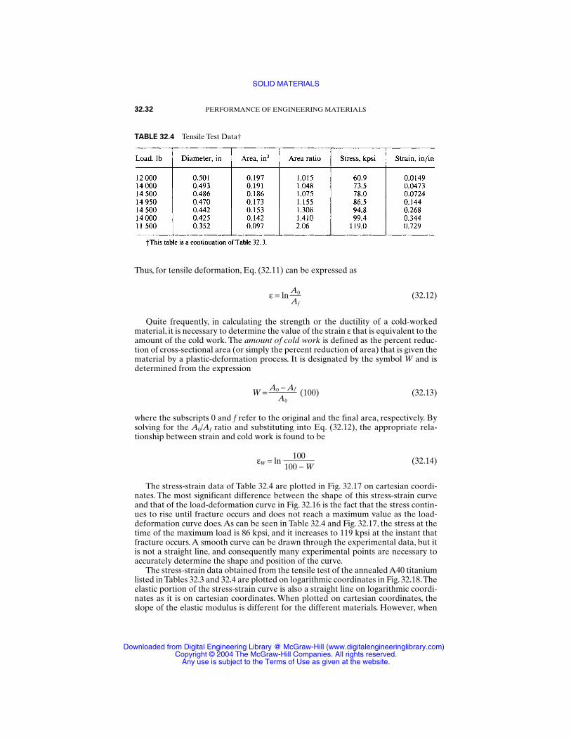
Thus, for tensile deformation, Eq. (32.11) can be expressed as
ε = ln (32.12)
Quite frequently, in calculating the strength or the ductility of a cold-workedmaterial, it is necessary to determine the value of the strain ε that is equivalent to theamount of the cold work. The amount of cold work is defined as the percent reduc-tion of cross-sectional area (or simply the percent reduction of area) that is given thematerial by a plastic-deformation process. It is designated by the symbol W and isdetermined from the expression
W = (100) (32.13)
where the subscripts 0 and f refer to the original and the final area, respectively. Bysolving for the A0/Af ratio and substituting into Eq. (32.12), the appropriate rela-tionship between strain and cold work is found to be
εW = ln 10
100−0
W (32.14)
The stress-strain data of Table 32.4 are plotted in Fig. 32.17 on cartesian coordi-nates. The most significant difference between the shape of this stress-strain curveand that of the load-deformation curve in Fig. 32.16 is the fact that the stress contin-ues to rise until fracture occurs and does not reach a maximum value as the load-deformation curve does. As can be seen in Table 32.4 and Fig. 32.17, the stress at thetime of the maximum load is 86 kpsi, and it increases to 119 kpsi at the instant thatfracture occurs. A smooth curve can be drawn through the experimental data, but itis not a straight line, and consequently many experimental points are necessary toaccurately determine the shape and position of the curve.
The stress-strain data obtained from the tensile test of the annealed A40 titaniumlisted in Tables 32.3 and 32.4 are plotted on logarithmic coordinates in Fig. 32.18.Theelastic portion of the stress-strain curve is also a straight line on logarithmic coordi-nates as it is on cartesian coordinates. When plotted on cartesian coordinates, theslope of the elastic modulus is different for the different materials. However, when
A0 − Af
A0
A0Af
32.32 PERFORMANCE OF ENGINEERING MATERIALS
TABLE 32.4 Tensile Test Data†
SOLID MATERIALS
Downloaded from Digital Engineering Library @ McGraw-Hill (www.digitalengineeringlibrary.com)Copyright © 2004 The McGraw-Hill Companies. All rights reserved.
Any use is subject to the Terms of Use as given at the website.
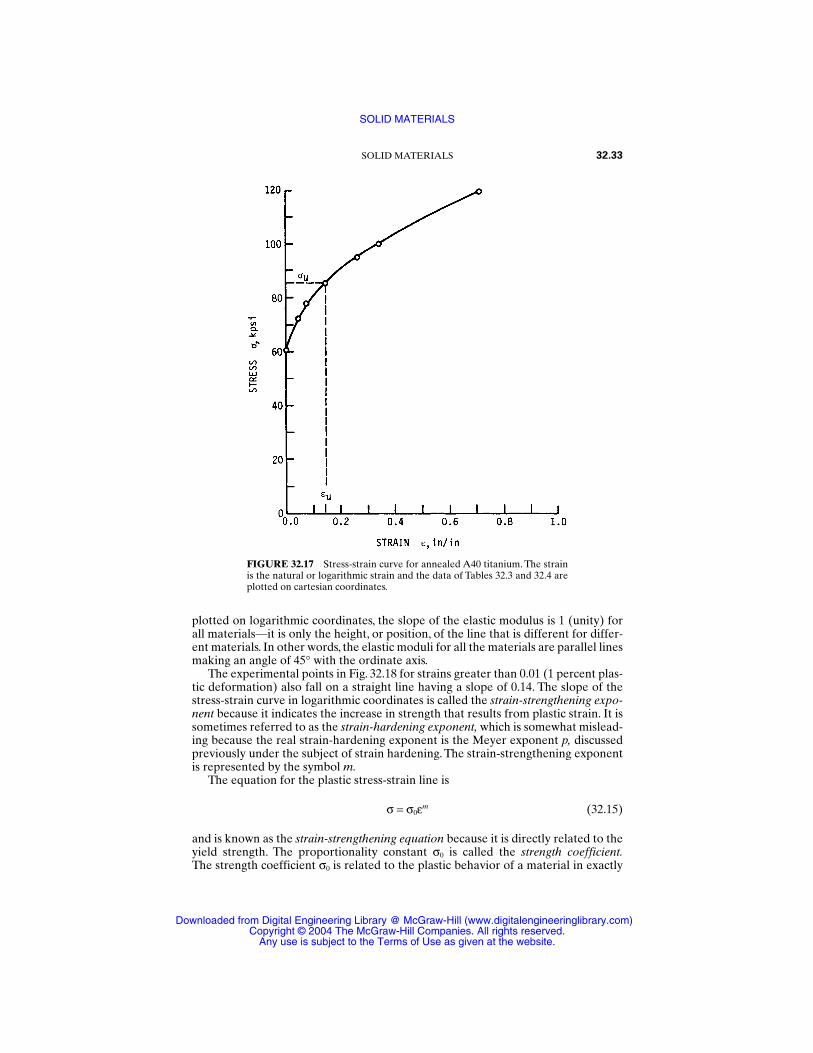
plotted on logarithmic coordinates, the slope of the elastic modulus is 1 (unity) forall materials—it is only the height, or position, of the line that is different for differ-ent materials. In other words, the elastic moduli for all the materials are parallel linesmaking an angle of 45° with the ordinate axis.
The experimental points in Fig. 32.18 for strains greater than 0.01 (1 percent plas-tic deformation) also fall on a straight line having a slope of 0.14. The slope of thestress-strain curve in logarithmic coordinates is called the strain-strengthening expo-nent because it indicates the increase in strength that results from plastic strain. It issometimes referred to as the strain-hardening exponent, which is somewhat mislead-ing because the real strain-hardening exponent is the Meyer exponent p, discussedpreviously under the subject of strain hardening. The strain-strengthening exponentis represented by the symbol m.
The equation for the plastic stress-strain line is
σ = σ0εm (32.15)
and is known as the strain-strengthening equation because it is directly related to theyield strength. The proportionality constant σ0 is called the strength coefficient.The strength coefficient σ0 is related to the plastic behavior of a material in exactly
SOLID MATERIALS 32.33
FIGURE 32.17 Stress-strain curve for annealed A40 titanium. The strainis the natural or logarithmic strain and the data of Tables 32.3 and 32.4 areplotted on cartesian coordinates.
SOLID MATERIALS
Downloaded from Digital Engineering Library @ McGraw-Hill (www.digitalengineeringlibrary.com)Copyright © 2004 The McGraw-Hill Companies. All rights reserved.
Any use is subject to the Terms of Use as given at the website.
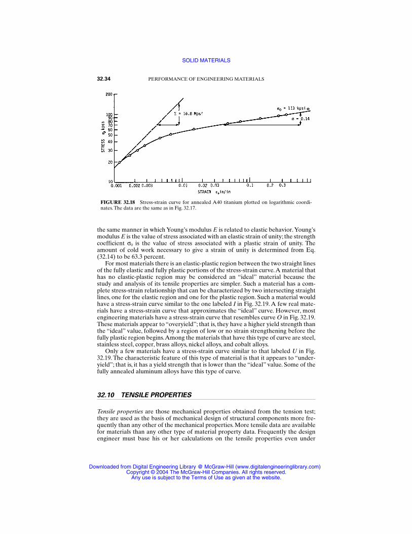
the same manner in which Young’s modulus E is related to elastic behavior.Young’smodulus E is the value of stress associated with an elastic strain of unity; the strengthcoefficient σ0 is the value of stress associated with a plastic strain of unity. Theamount of cold work necessary to give a strain of unity is determined from Eq.(32.14) to be 63.3 percent.
For most materials there is an elastic-plastic region between the two straight linesof the fully elastic and fully plastic portions of the stress-strain curve.A material thathas no elastic-plastic region may be considered an “ideal” material because thestudy and analysis of its tensile properties are simpler. Such a material has a com-plete stress-strain relationship that can be characterized by two intersecting straightlines, one for the elastic region and one for the plastic region. Such a material wouldhave a stress-strain curve similar to the one labeled I in Fig. 32.19. A few real mate-rials have a stress-strain curve that approximates the “ideal” curve. However, mostengineering materials have a stress-strain curve that resembles curve O in Fig. 32.19.These materials appear to “overyield”; that is, they have a higher yield strength thanthe “ideal” value, followed by a region of low or no strain strengthening before thefully plastic region begins.Among the materials that have this type of curve are steel,stainless steel, copper, brass alloys, nickel alloys, and cobalt alloys.
Only a few materials have a stress-strain curve similar to that labeled U in Fig.32.19. The characteristic feature of this type of material is that it appears to “under-yield”; that is, it has a yield strength that is lower than the “ideal” value. Some of thefully annealed aluminum alloys have this type of curve.
32.10 TENSILE PROPERTIES
Tensile properties are those mechanical properties obtained from the tension test;they are used as the basis of mechanical design of structural components more fre-quently than any other of the mechanical properties. More tensile data are availablefor materials than any other type of material property data. Frequently the designengineer must base his or her calculations on the tensile properties even under
32.34 PERFORMANCE OF ENGINEERING MATERIALS
FIGURE 32.18 Stress-strain curve for annealed A40 titanium plotted on logarithmic coordi-nates. The data are the same as in Fig. 32.17.
SOLID MATERIALS
Downloaded from Digital Engineering Library @ McGraw-Hill (www.digitalengineeringlibrary.com)Copyright © 2004 The McGraw-Hill Companies. All rights reserved.
Any use is subject to the Terms of Use as given at the website.
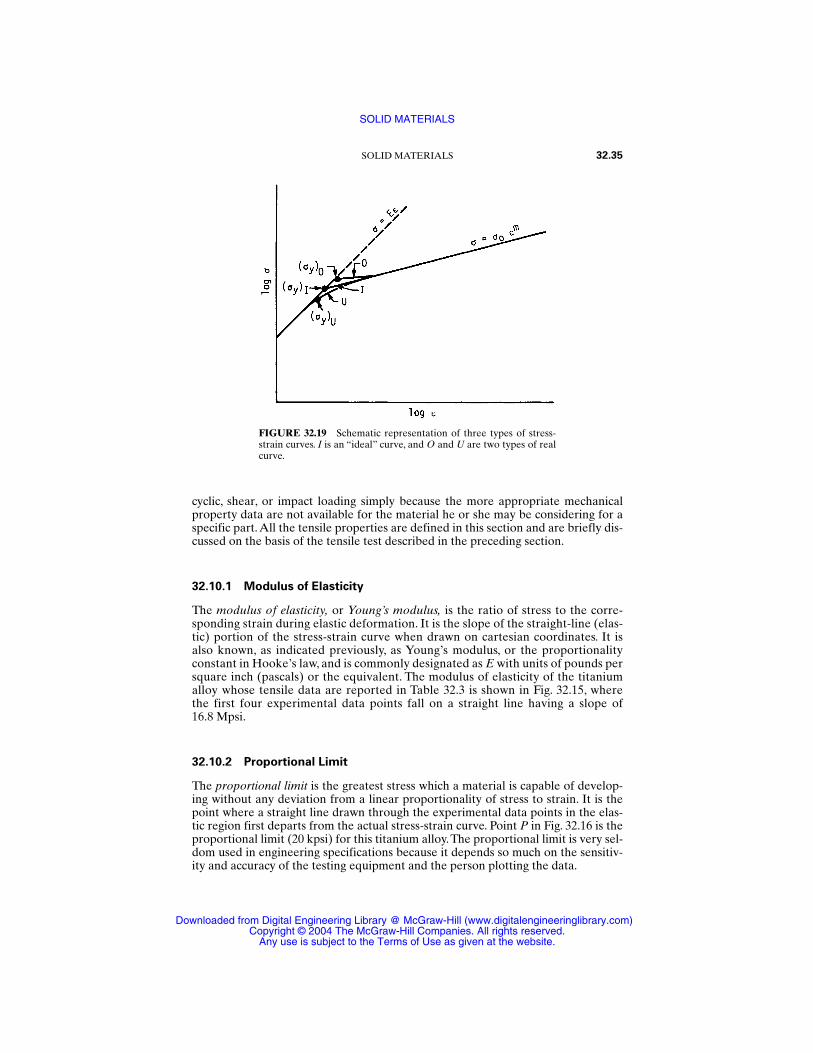
cyclic, shear, or impact loading simply because the more appropriate mechanicalproperty data are not available for the material he or she may be considering for aspecific part. All the tensile properties are defined in this section and are briefly dis-cussed on the basis of the tensile test described in the preceding section.
32.10.1 Modulus of Elasticity
The modulus of elasticity, or Young’s modulus, is the ratio of stress to the corre-sponding strain during elastic deformation. It is the slope of the straight-line (elas-tic) portion of the stress-strain curve when drawn on cartesian coordinates. It isalso known, as indicated previously, as Young’s modulus, or the proportionalityconstant in Hooke’s law, and is commonly designated as E with units of pounds persquare inch (pascals) or the equivalent. The modulus of elasticity of the titaniumalloy whose tensile data are reported in Table 32.3 is shown in Fig. 32.15, where the first four experimental data points fall on a straight line having a slope of 16.8 Mpsi.
32.10.2 Proportional Limit
The proportional limit is the greatest stress which a material is capable of develop-ing without any deviation from a linear proportionality of stress to strain. It is thepoint where a straight line drawn through the experimental data points in the elas-tic region first departs from the actual stress-strain curve. Point P in Fig. 32.16 is theproportional limit (20 kpsi) for this titanium alloy.The proportional limit is very sel-dom used in engineering specifications because it depends so much on the sensitiv-ity and accuracy of the testing equipment and the person plotting the data.
SOLID MATERIALS 32.35
FIGURE 32.19 Schematic representation of three types of stress-strain curves. I is an “ideal” curve, and O and U are two types of realcurve.
SOLID MATERIALS
Downloaded from Digital Engineering Library @ McGraw-Hill (www.digitalengineeringlibrary.com)Copyright © 2004 The McGraw-Hill Companies. All rights reserved.
Any use is subject to the Terms of Use as given at the website.

32.10.3 Elastic Limit
The elastic limit is the greatest stress which a material is capable of withstandingwithout any permanent deformation after removal of the load. It is designated aspoint Q in Fig. 32.16. The elastic limit is also very seldom used in engineering speci-fications because of the complex testing procedure of many successive loadings andunloadings that is necessary for its determination.
32.10.4 Yield Strength
The yield strength is the nominal stress at which a material undergoes a specifiedpermanent deformation. There are several methods to determine the yield strength,but the most reliable and consistent method is called the offset method. Thisapproach requires that the nominal stress-strain diagram be first drawn on cartesiancoordinates. A point z is placed along the strain axis at a specified distance from theorigin, as shown in Figs. 32.15 and 32.16. A line parallel to the elastic modulus isdrawn from Z until it intersects the nominal stress-strain curve. The value of stresscorresponding to this intersection is called the yield strength by the offset method.The distance 0Z is called the offset and is expressed as percent. The most commonoffset is 0.2 percent, which corresponds to a nominal strain of 0.002 in/in. This is thevalue of offset used in Fig. 32.15 to determine the yield strength of the A40 titanium.An offset of 0.01 percent is sometimes used, and the corresponding nominal stress iscalled the proof strength, which is a value very close to the proportional limit. Forsome nonferrous materials an offset of 0.5 percent is used to determine the yieldstrength.
Inasmuch as all methods of determining the yield strength give somewhat differ-ent values for the same material, it is important to specify what method, or what off-set, was used in conducting the test.
32.10.5 Tensile Strength
The tensile strength is the value of nominal stress obtained when the maximum (orultimate) load that the tensile specimen supports is divided by the original cross-sectional area of the specimen. It is shown as Su in Fig. 32.16 and is sometimes calledthe ultimate strength. The tensile strength is a commonly used property in engineer-ing calculations even though the yield strength is a measure of when plastic defor-mation begins for a given material. The real significance of the tensile strength as amaterial property is that it indicates what maximum load a given part can carry inuniaxial tension without breaking. It determines the absolute maximum limit of loadthat a part can support.
32.10.6 Fracture Strength
The fracture strength, or breaking strength, is the value of nominal stress obtainedwhen the load carried by a tensile specimen at the time of fracture is divided by itsoriginal cross-sectional area. The breaking strength is not used as a material prop-erty in mechanical design.
32.36 PERFORMANCE OF ENGINEERING MATERIALS
SOLID MATERIALS
Downloaded from Digital Engineering Library @ McGraw-Hill (www.digitalengineeringlibrary.com)Copyright © 2004 The McGraw-Hill Companies. All rights reserved.
Any use is subject to the Terms of Use as given at the website.
32.10.7 Reduction of Area
The reduction of area is the maximum change in area of a tensile specimen dividedby the original area and is usually expressed as a percent. It is designated as Ar andis calculated as follows:
Ar = (100) (32.16)
where the subscripts 0 and f refer to the original area and area after fracture, respec-tively. The percent reduction of area and the strain at ultimate load εu are the bestmeasure of the ductility of a material.
32.10.8 Fracture Strain
The fracture strain is the true strain at fracture of the tensile specimen. It is repre-sented by the symbol εf and is calculated from the definition of strain as given in Eq.(32.12). If the percent reduction of area Ar is known for a material, the fracturestrain can be calculated from the expression
εf = ln 100
10−0
Ar (32.17)
32.10.9 Percentage Elongation
The percentage elongation is a crude measure of the ductility of a material and isobtained when the change in gauge length of a fractured tensile specimen is dividedby the original gauge length and expressed as percent. Because of the ductility rela-tionship, we express it here as
De = f
−0
0 (100) (32.18)
Since most materials exhibit nonuniform deformation before fracture occurs on atensile test, the percentage elongation is some kind of an average value and as suchcannot be used in meaningful engineering calculations.
The percentage elongation is not really a material propety, but rather it is a com-bination of a material property and a test condition. A true material property is notsignificantly affected by the size of the specimen. Thus a 1⁄4-in-diameter and a 1⁄2-in-diameter tensile specimen of the same material give the same values for yieldstrength, tensile strength, reduction of area or fracture strain, modulus of elasticity,strain-strengthening exponent, and strength coefficient, but a 1-in gauge-lengthspecimen and a 2-in gauge-length specimen of the same material do not give thesame percentage elongation. In fact, the percentage elongation for a 1-in gauge-length specimen may actually be 100 percent greater than that for the 2-in gauge-length specimen even when they are of the same diameter.
A0 − Af
A0
SOLID MATERIALS 32.37
SOLID MATERIALS
Downloaded from Digital Engineering Library @ McGraw-Hill (www.digitalengineeringlibrary.com)Copyright © 2004 The McGraw-Hill Companies. All rights reserved.
Any use is subject to the Terms of Use as given at the website.
32.11 STRENGTH, STRESS, AND STRAIN RELATIONS
The following relationships between strength, stress, and strain are very helpful to acomplete understanding of tensile properties and also to an understanding of theiruse in specifying the optimum material for a structural part.These relationships alsohelp in solving manufacturing problems where difficulty is encountered in the fabri-cation of a given part because they enable one to have a better concept of what canbe expected of a material during a manufacturing process. A further advantage ofthese relations is that they enable an engineer to more readily determine themechanical properties of a fabricated part on the basis of the original properties ofthe material and the mechanisms involved with the particular process used.
32.11.1 Natural and Nominal Strain
The relationship between these two strains is determined from their definitions.Theexpression for the natural strain is ε = ln (f /0). The expression for the nominalstrain can be rewritten as f /0 = n + 1.When the latter is substituted into the former,the relationship between the two strains can be expressed in the two forms
ε = ln (n + 1) exp (ε) = n + 1 (32.19)
32.11.2 True and Nominal Stress
The definition of true stress is σ = L/Ai. From constancy of volume it is found that Ai = A0(0 /i), so that
σ = AL
0
0
iwhich is the same as
σ = S(n + 1) (32.20)S exp (ε)
32.11.3 Strain-Strengthening Exponent and Maximum-Load Strain
One of the more useful of the strength-stress-strain relationships is the one betweenthe strain-strengthening exponent and the strain at maximum load. It is also the sim-plest, since the two are numerically equal; that is, m = εu. This relation is derived onthe basis of the load-deformation curve shown in Fig. 32.20. The load at any pointalong this curve is equal to the product of the true stress on the specimen and thecorresponding area. Thus
L = σA
32.38 PERFORMANCE OF ENGINEERING MATERIALS
SOLID MATERIALS
Downloaded from Digital Engineering Library @ McGraw-Hill (www.digitalengineeringlibrary.com)Copyright © 2004 The McGraw-Hill Companies. All rights reserved.
Any use is subject to the Terms of Use as given at the website.
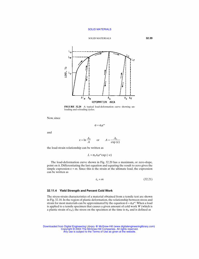
Now, since
σ = σ0εm
and
ε = ln AA
0 or A = ex
Ap
0
(ε)
the load-strain relationship can be written as
L = σ0A0εmexp (−ε)
The load-deformation curve shown in Fig. 32.20 has a maximum, or zero-slope,point on it. Differentiating the last equation and equating the result to zero gives thesimple expression ε = m. Since this is the strain at the ultimate load, the expressioncan be written as
εu = m (32.21)
32.11.4 Yield Strength and Percent Cold Work
The stress-strain characteristics of a material obtained from a tensile test are shownin Fig. 32.18. In the region of plastic deformation, the relationship between stress andstrain for most materials can be approximated by the equation σ = σ0εm.When a loadis applied to a tensile specimen that causes a given amount of cold work W (which isa plastic strain of εW), the stress on the specimen at the time is σW and is defined as
SOLID MATERIALS 32.39
FIGURE 32.20 A typical load-deformation curve showing un-loading and reloading cycles.
SOLID MATERIALS
Downloaded from Digital Engineering Library @ McGraw-Hill (www.digitalengineeringlibrary.com)Copyright © 2004 The McGraw-Hill Companies. All rights reserved.
Any use is subject to the Terms of Use as given at the website.
σW = σ0(εW)m (32.22)
Of course, σW is also equal to the applied load LW divided by the actual cross-sectional area of the specimen AW.
If the preceding tensile specimen were immediately unloaded after reading LW,the cross-sectional area would increase to AW′ from AW because of the elastic recov-ery or springback that occurs when the load is removed. This elastic recovery isinsignificant for engineering calculations with regard to the strength or stresses ona part.
If the tensile specimen that has been stretched to a cross-sectional area of AW′ isnow reloaded, it will deform elastically until the load LW is approached. As the loadis increased above LW, the specimen will again deform plastically. This unloading-reloading cycle is shown graphically in Fig. 32.20. The yield load for this previouslycold-worked specimen before the reloading is AW′ . Therefore, the yield strength ofthe previously cold-worked (stretched) specimen is approximately
(Sy)W = LA
W
W′
But since AW′ = AW, then
(Sy)W = ALW
W
By comparing the preceding equations, it is apparent that
(Sy)W σW
And by substituting this last relationship into Eq. (32.22), we get
(Sy)W = σ0(εW)m (32.23)
Thus it is apparent that the plastic portion of the σ − ε curve is approximately the locusof yield strengths for a material as a function of the amount of cold work. This rela-tionship is valid only for the axial tensile yield strength after tensile deformation orfor the axial compressive yield strength after axial deformation.
32.11.5 Tensile Strength and Cold Work
It is believed by materials and mechanical-design engineers that the only relation-ships between the tensile strength of a cold-worked material and the amount of coldwork given it are the experimentally determined tables and graphs that are providedby the material manufacturers and that the results are different for each family ofmaterials. However, on the basis of the concepts of the tensile test presented here,two relations are derived in Ref. [32.1] between tensile strength and percent coldwork that are valid when the prior cold work is tensile. These relations are derivedon the basis of the load-deformation characteristics of a material as represented inFig. 32.20. This model is valid for all metals that do not strain age.
Here we designate the tensile strength of a cold-worked material as (Su)W, and weare interested in obtaining the relationship to the percent cold work W. For any
32.40 PERFORMANCE OF ENGINEERING MATERIALS
SOLID MATERIALS
Downloaded from Digital Engineering Library @ McGraw-Hill (www.digitalengineeringlibrary.com)Copyright © 2004 The McGraw-Hill Companies. All rights reserved.
Any use is subject to the Terms of Use as given at the website.
specimen that is given a tensile deformation such that AW is equal to or less than Au,we have, by definition, that
(Su)W =
And also, by definition,
Lu = A0(Su)0
where (Su)0 = tensile strength of the original non-cold-worked specimen and A0 = itsoriginal area.
The percent cold work associated with the deformation of the specimen from A0
to AW′ is
W = (100) or w =
where w = W/100. Thus
AW′ = A0(1 − w)
By substitution into the first equation,
(Su)W = A
A
0(0
1(S
−u)w0
) =
1(S
−u)w0 (32.24)
Of course, this expression can also be expressed in the form
(Su)W = (Su)0 exp (ε) (32.25)
Thus the tensile strength of a material that is prestrained in tension to a strain less thanits ultimate load strain is equal to its original tensile strength divided by 1 minus thefraction of cold work. This relationship is valid for deformations less than the defor-mation associated with the ultimate load, that is, for
AW ≤ Au or εW ≤ εu
Another relationship can be derived for the tensile strength of a material that hasbeen previously cold-worked in tension by an amount greater than the deformationassociated with the ultimate load. This analysis is again made on the basis of Fig.32.20. Consider another standard tensile specimen of 1020 steel that is loadedbeyond Lu (12 000 lb) to some load Lz, say, 10 000 lb. If dead weights were placed onthe end of the specimen, it would break catastrophically when the 12 000-lb load wasapplied. But if the load had been applied by means of a mechanical screw or ahydraulic pump, then the load would drop off slowly as the specimen is stretched.For this particular example the load is considered to be removed instantly when itdrops to Lz or 10 000 lb.The unloaded specimen is not broken, although it may havea “necked” region, and it has a minimum cross-sectional area Az = 0.100 in2 and adiameter of 0.358 in. Now when this same specimen is again loaded in tension, it
A0 − AW′A0
A0 − AW′A0
LuAW′
SOLID MATERIALS 32.41
SOLID MATERIALS
Downloaded from Digital Engineering Library @ McGraw-Hill (www.digitalengineeringlibrary.com)Copyright © 2004 The McGraw-Hill Companies. All rights reserved.
Any use is subject to the Terms of Use as given at the website.
deforms elastically until the load reaches Lz (10 000 lb) and then it deforms plasti-cally. But Lz is also the maximum value of load that this specimen reaches on reload-ing. It never again will support a load of Lu = 12 000 lb. On this basis, the yieldstrength of this specimen is
(Sy)W = = 100.100010
= 99 200 psi
And the tensile strength of this previously deformed specimen is
(Su)W = ALz
z =
100.100010
= 99 200 psi
32.11.6 Ratio of Tensile Strength to Brinell Hardness
It is commonly known by mechanical-design engineers that the tensile strength of asteel can be estimated by multiplying its Brinell hardness number by 500. As statedearlier, this fact led to the wide acceptance of the Brinell hardness scale. However,this ratio is not 500 for all materials—it varies from as low as 450 to as high as 1000for the commonly used metals. The ratio of the tensile strength of a material to itsBrinell hardness number is identified by the symbol KB, and it is a function of boththe load used to determine the hardness and the strain-strengthening exponent ofthe material.
Since the Brinell hardness number of a given material is not a constant but variesin proportion to the applied load, it then follows that the proportionality coefficientKB is not a constant for a given material, but it too varies in proportion to the loadused in determining the hardness. For example, a 50 percent cobalt alloy (L605 orHS25) has a Brinell hardness number of 201 when tested with a 3000-kg load and ahardness of only 150 when tested with a 500-kg load. Since the tensile strength isabout 145 000 psi for this annealed alloy, the value for KB is about 970 for the lowload and about 730 for the high load.
Since the material is subjected to considerable plastic deformation when both thetensile strength and the Brinell hardness are measured, these two values are influ-enced by the strain-strengthening exponent m for the material. Therefore, KB mustalso be a function of m.
Figure 32.21 is a plot of experimental data obtained by this author over a numberof years that shows the relationships between the ratio KB and the two variablesstrain-strengthening exponent m and diameter of the indentation, which is a func-tion of the applied load. From these curves it is apparent that KB varies directly withm and inversely with the load or diameter of the indentation d. The following exam-ples will illustrate the applicability of these curves.
A test was conducted on a heat of alpha brass to see how accurately the tensilestrength of a material could be predicted from a hardness test when the strain-strengthening exponent of the material is not known. Loads varying from 200 to2000 kg were applied to a 10-mm ball, with the following results:
Load, kg 200 500 1000 1500 2000Diameter, mm 2.53 3.65 4.82 5.68 6.30
LzAz′
32.42 PERFORMANCE OF ENGINEERING MATERIALS
SOLID MATERIALS
Downloaded from Digital Engineering Library @ McGraw-Hill (www.digitalengineeringlibrary.com)Copyright © 2004 The McGraw-Hill Companies. All rights reserved.
Any use is subject to the Terms of Use as given at the website.
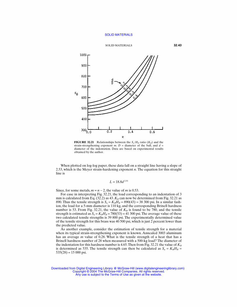
When plotted on log-log paper, these data fall on a straight line having a slope of2.53, which is the Meyer strain-hardening exponent n. The equation for this straightline is
L = 18.8d 2.53
Since, for some metals, m = n − 2, the value of m is 0.53.For ease in interpreting Fig. 32.21, the load corresponding to an indentation of 3
mm is calculated from Eq. (32.2) as 43. KB can now be determined from Fig. 32.21 as890. Thus the tensile strength is Su = KBHB = 890(43) = 38 300 psi. In a similar fash-ion, the load for a 5-mm diameter is 110 kg, and the corresponding Brinell hardnessnumber is 53. From Fig. 32.21, the value of KB is found to be 780, and the tensilestrength is estimated as Su = KBHB = 780(53) = 41 300 psi.The average value of thesetwo calculated tensile strengths is 39 800 psi. The experimentally determined valueof the tensile strength for this brass was 40 500 psi, which is just 2 percent lower thanthe predicted value.
As another example, consider the estimation of tensile strength for a materialwhen its typical strain-strengthening exponent is known. Annealed 3003 aluminumhas an average m value of 0.28. What is the tensile strength of a heat that has aBrinell hardness number of 28 when measured with a 500-kg load? The diameter ofthe indentation for this hardness number is 4.65.Then from Fig. 32.21 the value of KB
is determined as 535. The tensile strength can then be calculated as Su = KBHB =535(28) = 15 000 psi.
SOLID MATERIALS 32.43
FIGURE 32.21 Relationships between the Su /HB ratio (KB) and thestrain-strengthening exponent m. D = diameter of the ball, and d =diameter of the indentation. Data are based on experimental resultsobtained by the author.
SOLID MATERIALS
Downloaded from Digital Engineering Library @ McGraw-Hill (www.digitalengineeringlibrary.com)Copyright © 2004 The McGraw-Hill Companies. All rights reserved.
Any use is subject to the Terms of Use as given at the website.
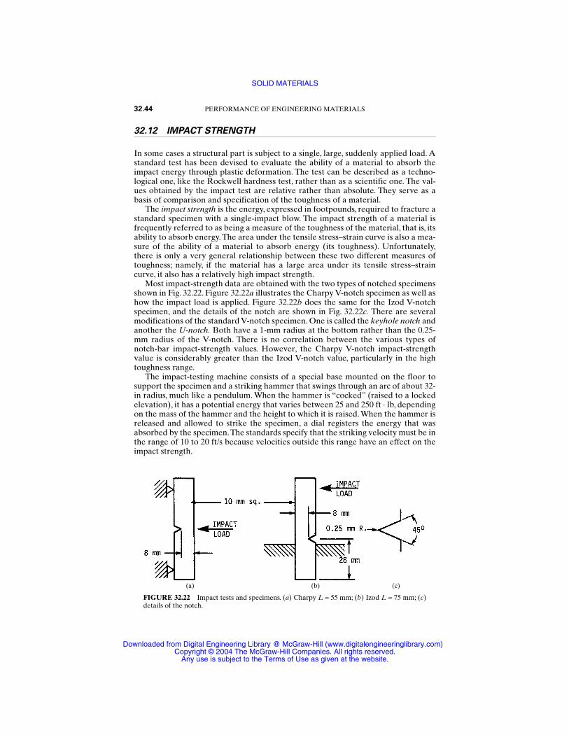
32.12 IMPACT STRENGTH
In some cases a structural part is subject to a single, large, suddenly applied load. Astandard test has been devised to evaluate the ability of a material to absorb theimpact energy through plastic deformation. The test can be described as a techno-logical one, like the Rockwell hardness test, rather than as a scientific one. The val-ues obtained by the impact test are relative rather than absolute. They serve as abasis of comparison and specification of the toughness of a material.
The impact strength is the energy, expressed in footpounds, required to fracture astandard specimen with a single-impact blow. The impact strength of a material isfrequently referred to as being a measure of the toughness of the material, that is, itsability to absorb energy. The area under the tensile stress–strain curve is also a mea-sure of the ability of a material to absorb energy (its toughness). Unfortunately,there is only a very general relationship between these two different measures oftoughness; namely, if the material has a large area under its tensile stress–straincurve, it also has a relatively high impact strength.
Most impact-strength data are obtained with the two types of notched specimensshown in Fig. 32.22. Figure 32.22a illustrates the Charpy V-notch specimen as well ashow the impact load is applied. Figure 32.22b does the same for the Izod V-notchspecimen, and the details of the notch are shown in Fig. 32.22c. There are severalmodifications of the standard V-notch specimen. One is called the keyhole notch andanother the U-notch. Both have a 1-mm radius at the bottom rather than the 0.25-mm radius of the V-notch. There is no correlation between the various types ofnotch-bar impact-strength values. However, the Charpy V-notch impact-strengthvalue is considerably greater than the Izod V-notch value, particularly in the hightoughness range.
The impact-testing machine consists of a special base mounted on the floor tosupport the specimen and a striking hammer that swings through an arc of about 32-in radius, much like a pendulum. When the hammer is “cocked” (raised to a lockedelevation), it has a potential energy that varies between 25 and 250 ft ⋅ lb, dependingon the mass of the hammer and the height to which it is raised. When the hammer isreleased and allowed to strike the specimen, a dial registers the energy that wasabsorbed by the specimen.The standards specify that the striking velocity must be inthe range of 10 to 20 ft/s because velocities outside this range have an effect on theimpact strength.
32.44 PERFORMANCE OF ENGINEERING MATERIALS
FIGURE 32.22 Impact tests and specimens. (a) Charpy L = 55 mm; (b) Izod L = 75 mm; (c)details of the notch.
(a) (b) (c)
SOLID MATERIALS
Downloaded from Digital Engineering Library @ McGraw-Hill (www.digitalengineeringlibrary.com)Copyright © 2004 The McGraw-Hill Companies. All rights reserved.
Any use is subject to the Terms of Use as given at the website.
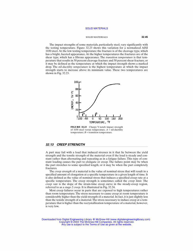
The impact strengths of some materials, particularly steel, vary significantly withthe testing temperature. Figure 32.23 shows this variation for a normalized AISI1030 steel. At the low testing temperature the fracture is of the cleavage type, whichhas a bright, faceted appearance.At the higher temperatures the fractures are of theshear type, which has a fibrous appearance. The transition temperature is that tem-perature that results in 50 percent cleavage fracture and 50 percent shear fracture, orit may be defined as the temperature at which the impact strength shows a markeddrop. The nil-ductility temperature is the highest temperature at which the impactstrength starts to increase above its minimum value. These two temperatures areshown in Fig. 32.23.
SOLID MATERIALS 32.45
FIGURE 32.23 Charpy V-notch impact strengthof 1030 steel versus temperature. A = nil-ductilitytemperature; B = transition temperature.
32.13 CREEP STRENGTH
A part may fail with a load that induced stresses in it that lie between the yieldstrength and the tensile strength of the material even if the load is steady and con-stant rather than alternating and repeating as in a fatigue failure. This type of con-stant loading causes the part to elongate or creep. The failure point may be whenthe part stretches to some specified length, or it may be when the part completelyfractures.
The creep strength of a material is the value of nominal stress that will result in aspecified amount of elongation at a specific temperature in a given length of time. Itis also defined as the value of nominal stress that induces a specified creep rate at aspecific temperature. The creep strength is sometimes called the creep limit. Thecreep rate is the slope of the strain-time creep curve in the steady-creep region,referred to as a stage 2 creep. It is illustrated in Fig. 32.24.
Most creep failures occur in parts that are exposed to high temperatures ratherthan room temperature. The stress necessary to cause creep at room temperature isconsiderably higher than the yield strength of a material. In fact, it is just slightly lessthan the tensile strength of a material.The stress necessary to induce creep at a tem-perature that is higher than the recrystallization temperature of a material, however,is very low.
SOLID MATERIALS
Downloaded from Digital Engineering Library @ McGraw-Hill (www.digitalengineeringlibrary.com)Copyright © 2004 The McGraw-Hill Companies. All rights reserved.
Any use is subject to the Terms of Use as given at the website.
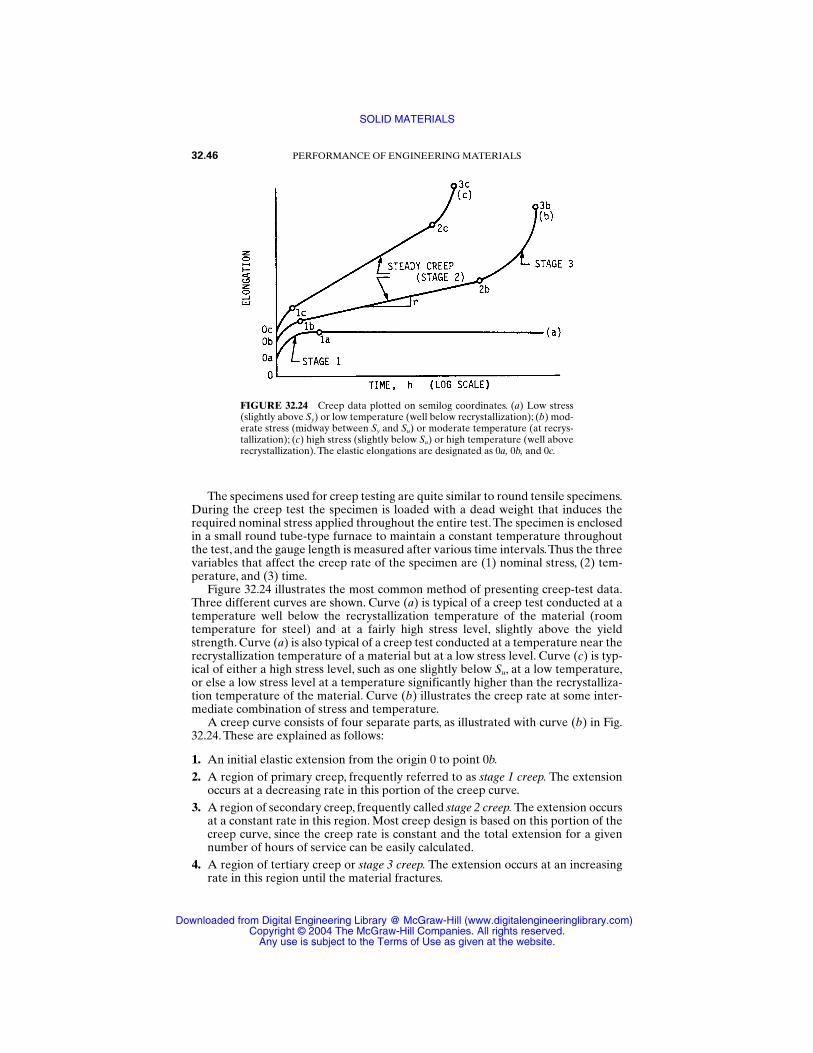
The specimens used for creep testing are quite similar to round tensile specimens.During the creep test the specimen is loaded with a dead weight that induces therequired nominal stress applied throughout the entire test.The specimen is enclosedin a small round tube-type furnace to maintain a constant temperature throughoutthe test, and the gauge length is measured after various time intervals.Thus the threevariables that affect the creep rate of the specimen are (1) nominal stress, (2) tem-perature, and (3) time.
Figure 32.24 illustrates the most common method of presenting creep-test data.Three different curves are shown. Curve (a) is typical of a creep test conducted at atemperature well below the recrystallization temperature of the material (roomtemperature for steel) and at a fairly high stress level, slightly above the yieldstrength. Curve (a) is also typical of a creep test conducted at a temperature near therecrystallization temperature of a material but at a low stress level. Curve (c) is typ-ical of either a high stress level, such as one slightly below Su, at a low temperature,or else a low stress level at a temperature significantly higher than the recrystalliza-tion temperature of the material. Curve (b) illustrates the creep rate at some inter-mediate combination of stress and temperature.
A creep curve consists of four separate parts, as illustrated with curve (b) in Fig.32.24. These are explained as follows:
1. An initial elastic extension from the origin 0 to point 0b.
2. A region of primary creep, frequently referred to as stage 1 creep. The extensionoccurs at a decreasing rate in this portion of the creep curve.
3. A region of secondary creep, frequently called stage 2 creep. The extension occursat a constant rate in this region. Most creep design is based on this portion of thecreep curve, since the creep rate is constant and the total extension for a givennumber of hours of service can be easily calculated.
4. A region of tertiary creep or stage 3 creep. The extension occurs at an increasingrate in this region until the material fractures.
32.46 PERFORMANCE OF ENGINEERING MATERIALS
FIGURE 32.24 Creep data plotted on semilog coordinates. (a) Low stress(slightly above Sy) or low temperature (well below recrystallization); (b) mod-erate stress (midway between Sy and Su) or moderate temperature (at recrys-tallization); (c) high stress (slightly below Su) or high temperature (well aboverecrystallization). The elastic elongations are designated as 0a, 0b, and 0c.
SOLID MATERIALS
Downloaded from Digital Engineering Library @ McGraw-Hill (www.digitalengineeringlibrary.com)Copyright © 2004 The McGraw-Hill Companies. All rights reserved.
Any use is subject to the Terms of Use as given at the website.
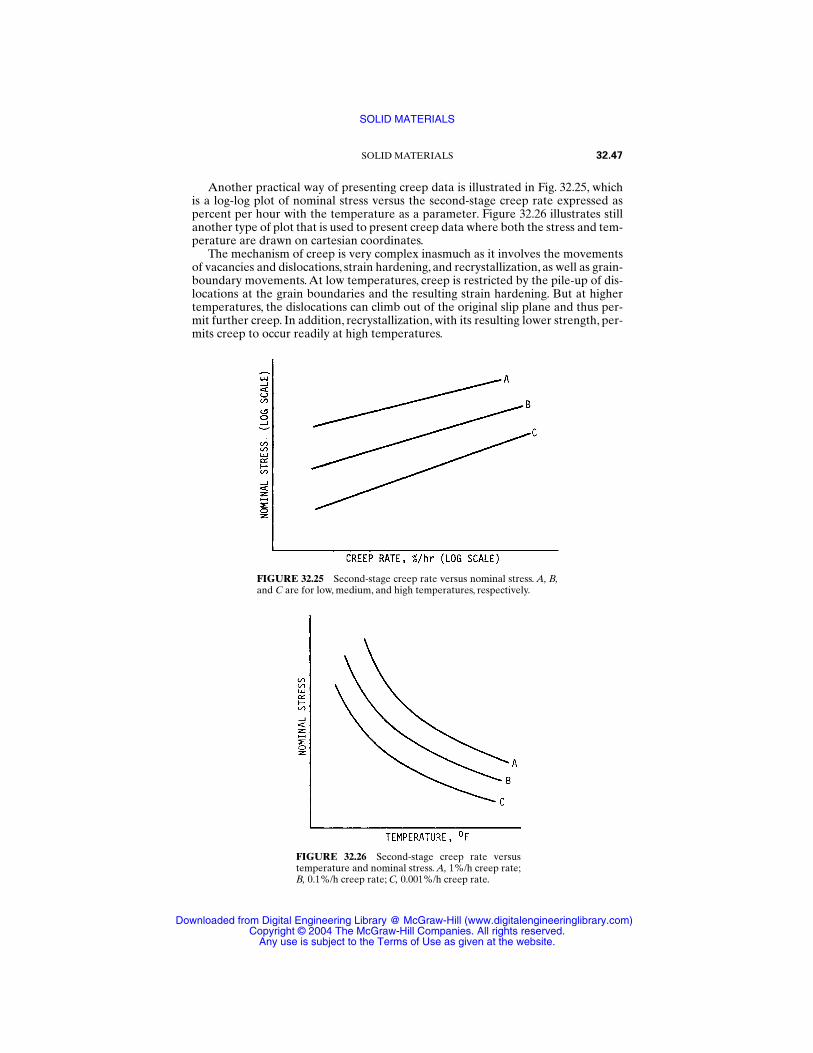
Another practical way of presenting creep data is illustrated in Fig. 32.25, whichis a log-log plot of nominal stress versus the second-stage creep rate expressed aspercent per hour with the temperature as a parameter. Figure 32.26 illustrates stillanother type of plot that is used to present creep data where both the stress and tem-perature are drawn on cartesian coordinates.
The mechanism of creep is very complex inasmuch as it involves the movementsof vacancies and dislocations, strain hardening, and recrystallization, as well as grain-boundary movements. At low temperatures, creep is restricted by the pile-up of dis-locations at the grain boundaries and the resulting strain hardening. But at highertemperatures, the dislocations can climb out of the original slip plane and thus per-mit further creep. In addition, recrystallization, with its resulting lower strength, per-mits creep to occur readily at high temperatures.
SOLID MATERIALS 32.47
FIGURE 32.25 Second-stage creep rate versus nominal stress. A, B,and C are for low, medium, and high temperatures, respectively.
FIGURE 32.26 Second-stage creep rate versustemperature and nominal stress. A, 1%/h creep rate;B, 0.1%/h creep rate; C, 0.001%/h creep rate.
SOLID MATERIALS
Downloaded from Digital Engineering Library @ McGraw-Hill (www.digitalengineeringlibrary.com)Copyright © 2004 The McGraw-Hill Companies. All rights reserved.
Any use is subject to the Terms of Use as given at the website.
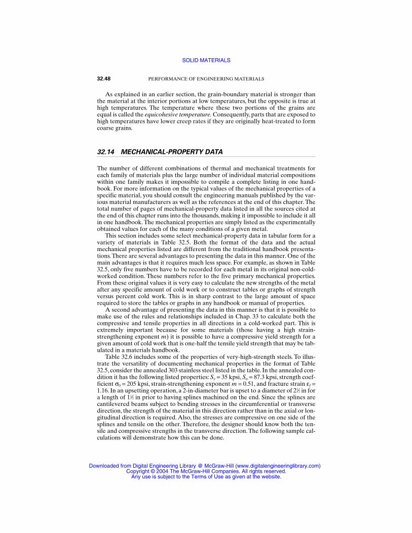
As explained in an earlier section, the grain-boundary material is stronger thanthe material at the interior portions at low temperatures, but the opposite is true athigh temperatures. The temperature where these two portions of the grains areequal is called the equicohesive temperature. Consequently, parts that are exposed tohigh temperatures have lower creep rates if they are originally heat-treated to formcoarse grains.
32.14 MECHANICAL-PROPERTY DATA
The number of different combinations of thermal and mechanical treatments foreach family of materials plus the large number of individual material compositionswithin one family makes it impossible to compile a complete listing in one hand-book. For more information on the typical values of the mechanical properties of aspecific material, you should consult the engineering manuals published by the var-ious material manufacturers as well as the references at the end of this chapter. Thetotal number of pages of mechanical-property data listed in all the sources cited atthe end of this chapter runs into the thousands, making it impossible to include it allin one handbook. The mechanical properties are simply listed as the experimentallyobtained values for each of the many conditions of a given metal.
This section includes some select mechanical-property data in tabular form for avariety of materials in Table 32.5. Both the format of the data and the actualmechanical properties listed are different from the traditional handbook presenta-tions.There are several advantages to presenting the data in this manner. One of themain advantages is that it requires much less space. For example, as shown in Table32.5, only five numbers have to be recorded for each metal in its original non-cold-worked condition. These numbers refer to the five primary mechanical properties.From these original values it is very easy to calculate the new strengths of the metalafter any specific amount of cold work or to construct tables or graphs of strengthversus percent cold work. This is in sharp contrast to the large amount of spacerequired to store the tables or graphs in any handbook or manual of properties.
A second advantage of presenting the data in this manner is that it is possible tomake use of the rules and relationships included in Chap. 33 to calculate both thecompressive and tensile properties in all directions in a cold-worked part. This isextremely important because for some materials (those having a high strain-strengthening exponent m) it is possible to have a compressive yield strength for agiven amount of cold work that is one-half the tensile yield strength that may be tab-ulated in a materials handbook.
Table 32.6 includes some of the properties of very-high-strength steels. To illus-trate the versatility of documenting mechanical properties in the format of Table32.5, consider the annealed 303 stainless steel listed in the table. In the annealed con-dition it has the following listed properties: Sy = 35 kpsi, Su = 87.3 kpsi, strength coef-ficient σ0 = 205 kpsi, strain-strengthening exponent m = 0.51, and fracture strain εf =1.16. In an upsetting operation, a 2-in-diameter bar is upset to a diameter of 21⁄2 in fora length of 11⁄2 in prior to having splines machined on the end. Since the splines arecantilevered beams subject to bending stresses in the circumferential or transversedirection, the strength of the material in this direction rather than in the axial or lon-gitudinal direction is required. Also, the stresses are compressive on one side of thesplines and tensile on the other. Therefore, the designer should know both the ten-sile and compressive strengths in the transverse direction. The following sample cal-culations will demonstrate how this can be done.
32.48 PERFORMANCE OF ENGINEERING MATERIALS
SOLID MATERIALS
Downloaded from Digital Engineering Library @ McGraw-Hill (www.digitalengineeringlibrary.com)Copyright © 2004 The McGraw-Hill Companies. All rights reserved.
Any use is subject to the Terms of Use as given at the website.
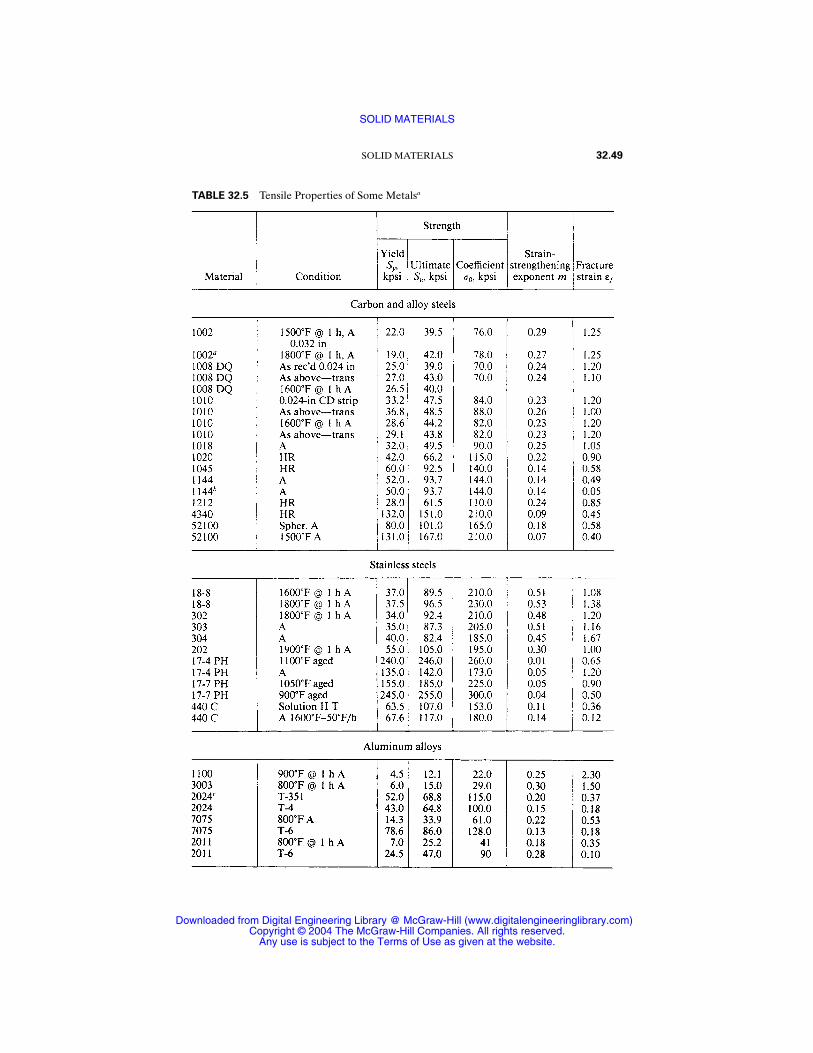
SOLID MATERIALS 32.49
TABLE 32.5 Tensile Properties of Some Metalsa
SOLID MATERIALS
Downloaded from Digital Engineering Library @ McGraw-Hill (www.digitalengineeringlibrary.com)Copyright © 2004 The McGraw-Hill Companies. All rights reserved.
Any use is subject to the Terms of Use as given at the website.
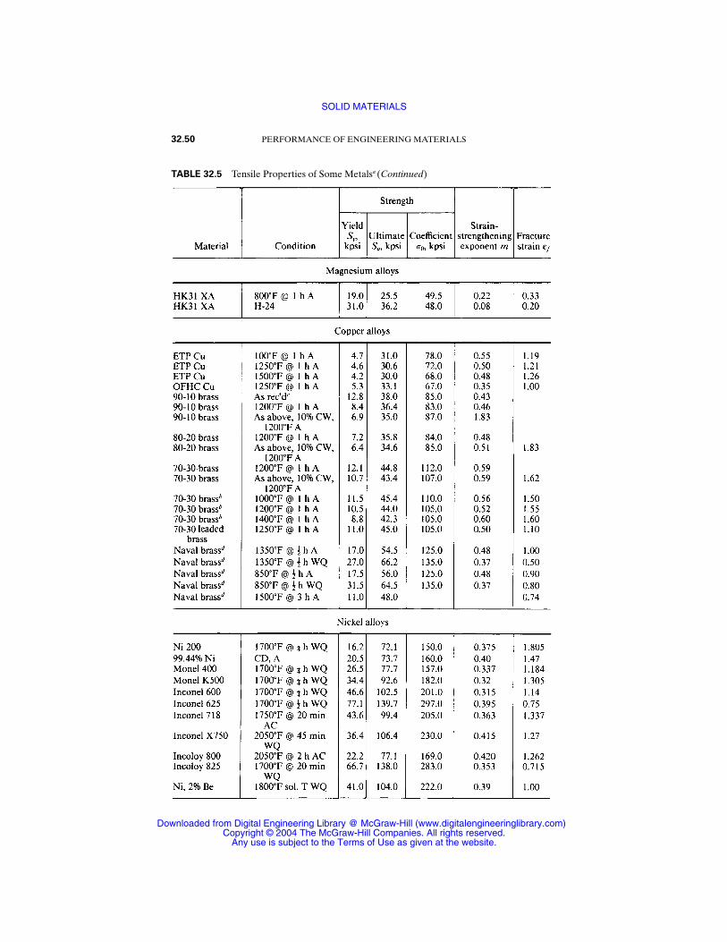
32.50 PERFORMANCE OF ENGINEERING MATERIALS
TABLE 32.5 Tensile Properties of Some Metalsa (Continued)
SOLID MATERIALS
Downloaded from Digital Engineering Library @ McGraw-Hill (www.digitalengineeringlibrary.com)Copyright © 2004 The McGraw-Hill Companies. All rights reserved.
Any use is subject to the Terms of Use as given at the website.
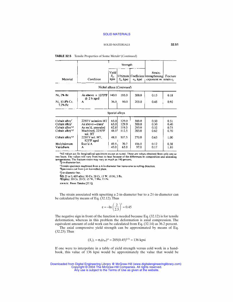
The strain associated with upsetting a 2-in-diameter bar to a 21⁄2-in-diameter canbe calculated by means of Eq. (32.12). Thus
ε = −ln 22.5
2
= 0.45
The negative sign in front of the function is needed because Eq. (32.12) is for tensiledeformation, whereas in this problem the deformation is axial compression. Theequivalent amount of cold work can be calculated from Eq. (32.14) as 36.2 percent.
The axial compressive yield strength can be approximated by means of Eq.(32.23). Thus
(Sy)c = σ0(εW)m = 205(0.45)0.51 = 136 kpsi
If one were to interpolate in a table of yield strength versus cold work in a hand-book, this value of 136 kpsi would be approximately the value that would be
SOLID MATERIALS 32.51
TABLE 32.5 Tensile Properties of Some Metalsa (Continued)
SOLID MATERIALS
Downloaded from Digital Engineering Library @ McGraw-Hill (www.digitalengineeringlibrary.com)Copyright © 2004 The McGraw-Hill Companies. All rights reserved.
Any use is subject to the Terms of Use as given at the website.
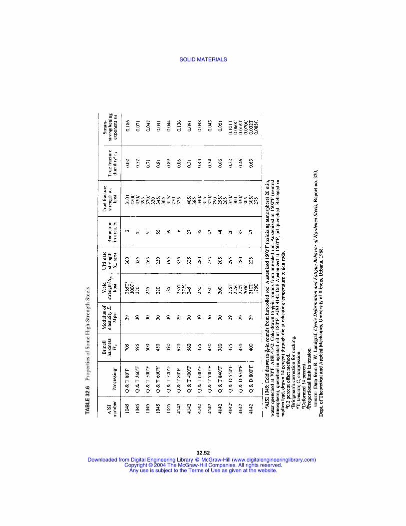
TA
BLE
32.6
Pro
pert
ies
of S
ome
Hig
h-St
reng
th S
teel
s
32.52
SOLID MATERIALS
Downloaded from Digital Engineering Library @ McGraw-Hill (www.digitalengineeringlibrary.com)Copyright © 2004 The McGraw-Hill Companies. All rights reserved.
Any use is subject to the Terms of Use as given at the website.
obtained for 36 percent cold work.And the handbook would not indicate whether itwas a compressive or tensile yield strength, nor in what direction it was applied.
However, for this problem, the designer really needs both the tensile and com-pressive yield strengths in the transverse, i.e., circumferential, direction.These valuescan be closely approximated by means of Table 33.1.The tensile yield strength in thetransverse direction is designated by the code (Sy)tTt, which is in group 2 of Table33.1. Since the bar was given only one cycle of deformation (a single upset), εqus is0.45 and the tensile yield strength is calculated to be 123 kpsi.The compressive yieldstrength in the transverse direction is designated by the code (Sy)cTt, which is ingroup 4 of Table 33.1. The compressive yield strength is then calculated to be0.95(Sy)tTt = 0.95(123) = 117 kpsi; this is 14 percent lower than the 136 kpsi that wouldnormally be listed in a materials handbook.
In some design situations, the actual value of the yield strength in a given part fora specific amount of cold work may be 50 percent less than the value that would belisted in the materials handbook. In order to have a reliable design, the designermust be able to determine the strength of the material in a part in the direction andsense of the induced stresses. The information in this chapter and in Chap. 33 makesit possible for the design engineer to make a reasonable prediction of the mechani-cal properties of a fabricated part. However, it must be recognized that the originalnon-cold-worked properties of a given metal vary from heat to heat, and that the cal-culations are valid only for a part having the original properties that are used in thecalculations.
32.15 NUMBERING SYSTEMS†
32.15.1 AISI and SAE Designation of Steel
Carbon and alloy steels are specified by a code consisting of a four-digit (some-times five) number, as illustrated below with the substitution of the letters X, Y,and Z for the numbers. A steel specification of XYZZ (or XYZZZ) has the fol-lowing meaning:
X indicates the type of alloy or alloys present.
Y indicates the total percent of the alloys present.
ZZ (or ZZZ) indicates the “points” of carbon in the steel (points of carbonequals the percent carbon times 100). For example, if ZZ is 40, then the steel has0.40 percent carbon (C). If ZZZ is 120, then the steel has 1.20 percent carbon.
Table 32.7 identifies the number X corresponding to the alloy or alloys present.In addition, the following two special classes are included. A resulfurized free-machining steel is identified as 11ZZ and 12ZZ. These steels have a high sulfur con-tent, which combines with the manganese to form the compound manganese sulfide.It is the presence of this compound that makes the steel more machinable.The 13ZZand 15ZZ groups are plain carbon steels that have high and moderate amounts ofmanganese, respectively.
SOLID MATERIALS 32.53
† This section presents the numbering systems now in general use in order to correspond with those usedin other sections of this handbook. See Ref. [32.2] for details of the unified numbering system (UNS).
SOLID MATERIALS
Downloaded from Digital Engineering Library @ McGraw-Hill (www.digitalengineeringlibrary.com)Copyright © 2004 The McGraw-Hill Companies. All rights reserved.
Any use is subject to the Terms of Use as given at the website.
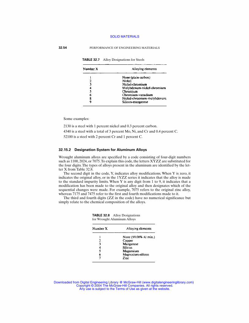
Some examples:
2130 is a steel with 1 percent nickel and 0.3 percent carbon.4340 is a steel with a total of 3 percent Mo, Ni, and Cr and 0.4 percent C.52100 is a steel with 2 percent Cr and 1 percent C.
32.15.2 Designation System for Aluminum Alloys
Wrought aluminum alloys are specified by a code consisting of four-digit numberssuch as 1100, 2024, or 7075.To explain this code, the letters XYZZ are substituted forthe four digits. The types of alloys present in the aluminum are identified by the let-ter X from Table 32.8.
The second digit in the code, Y, indicates alloy modifications. When Y is zero, itindicates the original alloy, or in the 1YZZ series it indicates that the alloy is madeto the standard impurity limits. When Y is any digit from 1 to 9, it indicates that amodification has been made to the original alloy and then designates which of thesequential changes were made. For example, 7075 refers to the original zinc alloy,whereas 7175 and 7475 refer to the first and fourth modifications made to it.
The third and fourth digits (ZZ in the code) have no numerical significance butsimply relate to the chemical composition of the alloys.
32.54 PERFORMANCE OF ENGINEERING MATERIALS
TABLE 32.7 Alloy Designations for Steels
TABLE 32.8 Alloy Designations for Wrought Aluminum Alloys
SOLID MATERIALS
Downloaded from Digital Engineering Library @ McGraw-Hill (www.digitalengineeringlibrary.com)Copyright © 2004 The McGraw-Hill Companies. All rights reserved.
Any use is subject to the Terms of Use as given at the website.
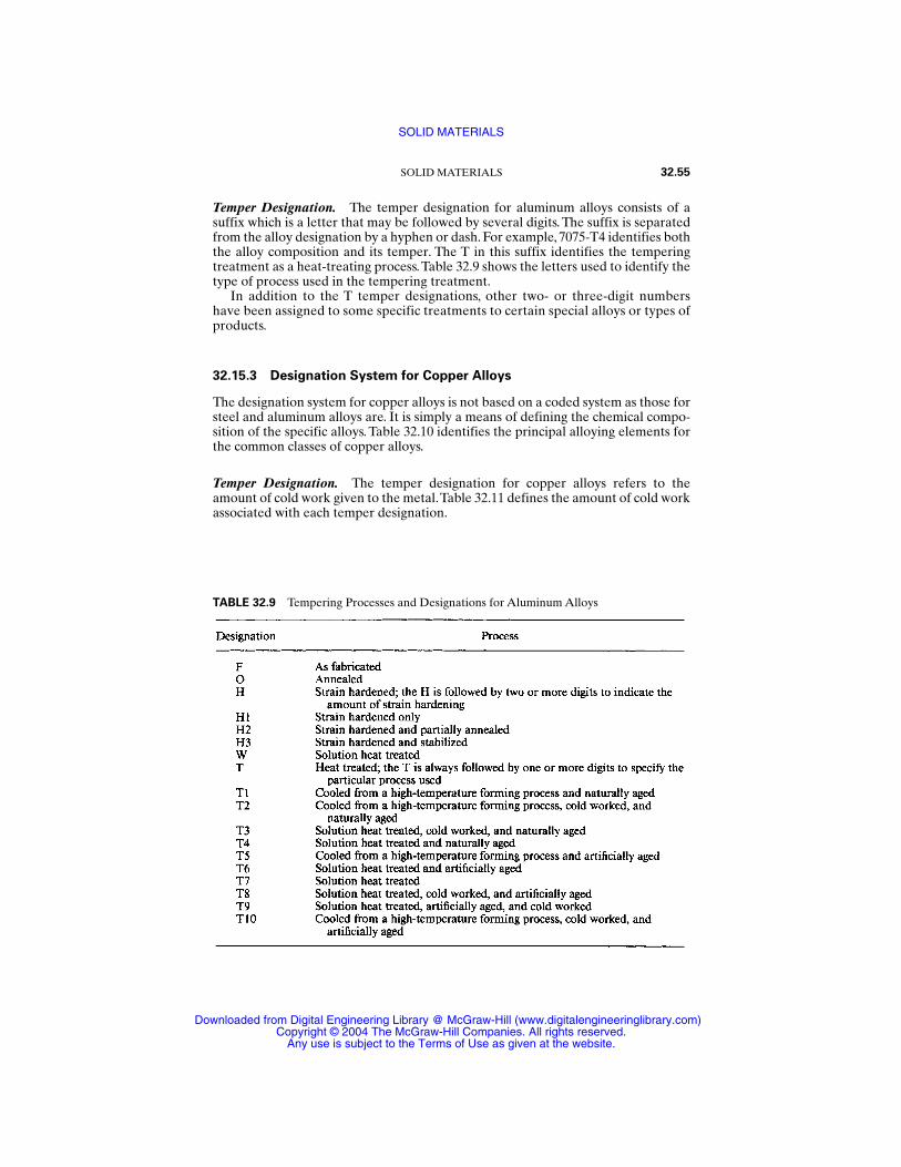
Temper Designation. The temper designation for aluminum alloys consists of asuffix which is a letter that may be followed by several digits. The suffix is separatedfrom the alloy designation by a hyphen or dash. For example, 7075-T4 identifies boththe alloy composition and its temper. The T in this suffix identifies the temperingtreatment as a heat-treating process.Table 32.9 shows the letters used to identify thetype of process used in the tempering treatment.
In addition to the T temper designations, other two- or three-digit numbershave been assigned to some specific treatments to certain special alloys or types ofproducts.
32.15.3 Designation System for Copper Alloys
The designation system for copper alloys is not based on a coded system as those forsteel and aluminum alloys are. It is simply a means of defining the chemical compo-sition of the specific alloys. Table 32.10 identifies the principal alloying elements forthe common classes of copper alloys.
Temper Designation. The temper designation for copper alloys refers to theamount of cold work given to the metal.Table 32.11 defines the amount of cold workassociated with each temper designation.
SOLID MATERIALS 32.55
TABLE 32.9 Tempering Processes and Designations for Aluminum Alloys
SOLID MATERIALS
Downloaded from Digital Engineering Library @ McGraw-Hill (www.digitalengineeringlibrary.com)Copyright © 2004 The McGraw-Hill Companies. All rights reserved.
Any use is subject to the Terms of Use as given at the website.
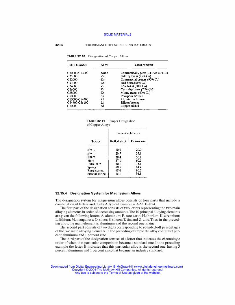
32.15.4 Designation System for Magnesium Alloys
The designation system for magnesium alloys consists of four parts that include acombination of letters and digits. A typical example is AZ31B-H24.
The first part of the designation consists of two letters representing the two mainalloying elements in order of decreasing amounts.The 10 principal alloying elementsare given the following letters:A, aluminum; E, rare earth; H, thorium; K, zirconium;L, lithium; M, manganese; Q, silver; S, silicon; T, tin; and Z, zinc. Thus, in the preced-ing alloy, the main element is aluminum and the second one is zinc.
The second part consists of two digits corresponding to rounded-off percentagesof the two main alloying elements. In the preceding example the alloy contains 3 per-cent aluminum and 1 percent zinc.
The third part of the designation consists of a letter that indicates the chronologicorder of when that particular composition became a standard one. In the precedingexample the letter B indicates that this particular alloy is the second one, having 3percent aluminum and 1 percent zinc, that became an industry standard.
32.56 PERFORMANCE OF ENGINEERING MATERIALS
TABLE 32.10 Designation of Copper Alloys
TABLE 32.11 Temper Designation of Copper Alloys
SOLID MATERIALS
Downloaded from Digital Engineering Library @ McGraw-Hill (www.digitalengineeringlibrary.com)Copyright © 2004 The McGraw-Hill Companies. All rights reserved.
Any use is subject to the Terms of Use as given at the website.

The fourth part consists of a letter preceded by a hyphen and followed by a num-ber. It indicates the specific condition or temper that the alloy is in.Table 32.12 spec-ifies the symbols that are used for each temper.
SOLID MATERIALS 32.57
REFERENCES
32.1 J. Datsko, Materials in Design and Manufacture, J. Datsko Consultants,Ann Arbor, Mich.,1978.
32.2 Metals and Alloys in the Unified Numbering System, 3d ed., Society of Automotive Engi-neers, Inc. (SAE), 1983.
32.3 Metals Handbook Desk Edition, American Society for Metals (ASM), Metals Park, Ohio,1984.
32.4 R. M. Brick,A.W. Pense, and R. B. Gordon, Structure and Properties of Engineering Mate-rials, 4th ed., McGraw-Hill, New York, 1977.
32.5 M. M. Schwartz, Composite Materials Handbook, McGraw-Hill, New York, 1984.
32.6 L. H. Van Vlack, Elements of Materials Science, 4th ed., Addison-Wesley, Reading, Mass.,1980.
TABLE 32.12 Temper Designation of Magnesium Alloys
SOLID MATERIALS
Downloaded from Digital Engineering Library @ McGraw-Hill (www.digitalengineeringlibrary.com)Copyright © 2004 The McGraw-Hill Companies. All rights reserved.
Any use is subject to the Terms of Use as given at the website.

SOLID MATERIALS
Downloaded from Digital Engineering Library @ McGraw-Hill (www.digitalengineeringlibrary.com)Copyright © 2004 The McGraw-Hill Companies. All rights reserved.
Any use is subject to the Terms of Use as given at the website.

CHAPTER 33THE STRENGTH
OF COLD-WORKED AND HEAT-TREATED STEELS
Charles R. Mischke, Ph.D., P.E.Professor Emeritus of Mechanical Engineering
Iowa State UniversityAmes, Iowa
33.1 INTRODUCTION / 33.2
33.2 STRENGTH OF PLASTICALLY DEFORMED MATERIALS / 33.3
33.3 ESTIMATING ULTIMATE STRENGTH AFTER PLASTIC STRAINS / 33.4
33.4 ESTIMATING YIELD STRENGTH AFTER PLASTIC STRAINS / 33.8
33.5 ESTIMATING ULTIMATE STRENGTH OF HEAT-TREATED
PLAIN CARBON STEELS / 33.9
33.6 ESTIMATING ULTIMATE STRENGTH OF HEAT-TREATED
LOW-ALLOY STEELS / 33.11
33.7 TEMPERING TIME AND TEMPERATURE TRADEOFF RELATION / 33.29
REFERENCES / 33.31
RECOMMENDED READING / 33.31
GLOSSARY
AR Fractional area reductionA AreaB Critical hardness for carbon content and tempering temperature,
Rockwell C scaled DiameterD Tempering decrement, Rockwell C scale; carbon ideal diameter, inDl Ideal critical diameter, inDH Distant hardness, Rockwell C scaleEJD Equivalent Jominy distance, sixteenths of inchf Tempering factor for carbon content and tempering temperatureF Load, temperature, degrees FahrenheitH Quench severity, in−1
IH Initial hardness, Rockwell C scale
33.1
Source: STANDARD HANDBOOK OF MACHINE DESIGN
Downloaded from Digital Engineering Library @ McGraw-Hill (www.digitalengineeringlibrary.com)Copyright © 2004 The McGraw-Hill Companies. All rights reserved.
Any use is subject to the Terms of Use as given at the website.

m Strain-strengthening exponentn Design factorr RadiusRmax Maximum hardness attainable, Rockwell C scaleRQ As-quenched Jominy test hardness, Rockwell C scaleRT Tempered hardness, Rockwell C scaleSe′ Engineering endurance limitSu Engineering ultimate strength in tensionSy Engineering yield strength, 0.2 percent offsett Timeε True strainη Factor of safetyσ0 Strain-strengthening coefficientσ Normal stressΣA Sum of alloy increments, Rockwell C scaleτo Octahedral shear stressτ Shearing stress
Subscripts
a AxialB Long traversec CompressionC CircumferentialD Short traversee Endurancef FractureL LongitudinalR Radials Sheart Tensionu Ultimatey Yield0 No prior strain
33.1 INTRODUCTION
The mechanical designer needs to know the yield strength of a material so that asuitable margin against permanent distortion can be provided. The yield strengthprovided by a standardized tensile test is often not helpful because the manufactur-
33.2 PERFORMANCE OF ENGINEERING MATERIALS
THE STRENGTH OF COLD-WORKED AND HEAT-TREATED STEELS
Downloaded from Digital Engineering Library @ McGraw-Hill (www.digitalengineeringlibrary.com)Copyright © 2004 The McGraw-Hill Companies. All rights reserved.
Any use is subject to the Terms of Use as given at the website.
ing process has altered this property. Hot or cold forming and heat treatment(quenching and tempering) change the yield strength. The designer needs to knowthe yield strength of the material at the critical location in the geometry and at con-dition of use.
The designer also needs knowledge of the ultimate strength, principally as anestimator of fatigue strength, so that a suitable margin against fracture or fatigue canbe provided. Hot and cold forming and various thermomechanical treatments dur-ing manufacture have altered these properties too. These changes vary within thepart and can be directional. Again, the designer needs strength information for thematerial at the critical location in the geometry and at condition of use.
This chapter addresses the effect of plastic strain or a sequence of plastic strainson changes in yield and ultimate strengths (and associated endurance limits) andgives quantitative methods for the estimation of these properties. It also examinesthe changes in ultimate strength in heat-treated plain carbon and low-alloy steels.
33.2 STRENGTH OF PLASTICALLY DEFORMED MATERIALS
Methods for strength estimation include the conventional uniaxial tension test,which routinely measures true and engineering yield and ultimate strengths, per-centage elongation and reduction in area, true ultimate and fracture strains, strain-strengthening exponent, strain-strengthening coefficient, and Young’s modulus.These results are for the material in specimen form. Machine parts are of differentshape, size, texture, material treatment, and manufacturing history and resist loadingdifferently. Hardness tests can be made on a prototype part, and from correlations ofstrength with hardness and indentor size ([33.1], p. 5–35) and surface, ultimatestrength can be assessed. Such information can be found in corporate manuals andcatalogs or scattered in the literature. Often these are not helpful.
In the case of a single plastic deformation in the manufacturing process, one canuse the true stress-strain curve of the material in the condition prior to straining pro-vided the plastic strain can be determined. The results are good. For a sequence ofsuccessive strains, an empirical method is available which approximates what hap-pens but is sometimes at variance with test results.
Cold work or strain strengthening is a common result of a cold-forming process.The process changes the properties, and such changes must be incorporated into theapplication of a theory of failure. The important strength is that of the part in thecritical location in the geometry and at condition of use.
33.2.1 Datsko’s Notation
In any discussion of strength it is necessary to identify
1. The kind of strength: ultimate, u; yield, y; fracture, f; endurance, e.
2. The sense of the strength: tensile, t; compressive, c; shear, s.
3. The direction or orientation of the strength: longitudinal, L; long transverse, B;short transverse, D; axial, a; radial, R; circumferential, C.
4. The sense of the most recent prior strain in the axial direction of the envisionedtest specimen: tension, t; compression, c. If there is no prior strain, the subscript 0is used.
THE STRENGTH OF COLD-WORKED AND HEAT-TREATED STEELS 33.3
THE STRENGTH OF COLD-WORKED AND HEAT-TREATED STEELS
Downloaded from Digital Engineering Library @ McGraw-Hill (www.digitalengineeringlibrary.com)Copyright © 2004 The McGraw-Hill Companies. All rights reserved.
Any use is subject to the Terms of Use as given at the website.
33.2.2 Datsko’s Rules
Datsko [33.1] suggests a notation (S1)234, where the subscripts correspond to 1, 2, 3,and 4 above. In Fig. 33.1 an axially deformed round and a rolled plate are depicted.A strength (Su)tLc would be read as the engineering ultimate strength Su, in tension(Su)t, in the longitudinal direction (Su)tL, after a last prior strain in the specimendirection that was compressive (Su)tLc. Datsko [33.1] has articulated rules for strainstrengthening that are in approximate agreement with data he has collected. Briefly,
Rule 1. Strain strengthening is a bulk mechanism, exhibiting changes in strengthin directions free of strain.Rule 2. The maximum strain that can be imposed lies between the true strain atultimate load εu and the true fracture strain εf. In upsetting procedures devoid offlexure, the limit is εf, as determined in the tension test.Rule 3. The significant strain in a deformation cycle is the largest absolute strain,denoted εw. In a round εw = max(|εr|, |εθ|, |εx|).The largest absolute strain εw is usedin calculating the equivalent plastic strain εq, which is defined for two categoriesof strength, ultimate and yield, and in four groups of strength in Table 33.1.Rule 4. In the case of several strains applied sequentially (say, cold rolling thenupsetting), in determining εqu, the significant strains in each cycle εwl are added indecreasing order of magnitude rather than in chronological order.Rule 5. If the plastic strain is imposed below the material’s recrystallization tem-perature, the ultimate tensile strength is given by
Su = (Su)o exp εqu εqu < m
= σ0(εqu)m εqu > m
Rule 6. The yield strength of a material whose recrystallization temperature wasnot exceeded is given by
Sy = σ0(εqy)m
Table 33.1 summarizes the strength relations for plastically deformed metals.
33.3 ESTIMATING ULTIMATE STRENGTH AFTER PLASTIC STRAINS
This topic is best illuminated by example, applying ideas expressed in Secs. 33.2.1and 33.2.2.
Example 1. A 1045HR bar has the following properties from tension tests:
Sy = 60 kpsi Su = 92.5 kpsi
AR = 0.44 m = 0.14
The material is to be used to form an integral pinion on a shaft by cold working from21⁄4 in to 2 in diameter and then upsetting to 21⁄2 in to form a pinion blank, as depictedin Fig. 33.2. Find, using Datsko’s rules, an estimate of the ultimate strength in a direc-tion resisting tooth bending at the root of the gear tooth to be cut in the blank.
33.4 PERFORMANCE OF ENGINEERING MATERIALS
THE STRENGTH OF COLD-WORKED AND HEAT-TREATED STEELS
Downloaded from Digital Engineering Library @ McGraw-Hill (www.digitalengineeringlibrary.com)Copyright © 2004 The McGraw-Hill Companies. All rights reserved.
Any use is subject to the Terms of Use as given at the website.
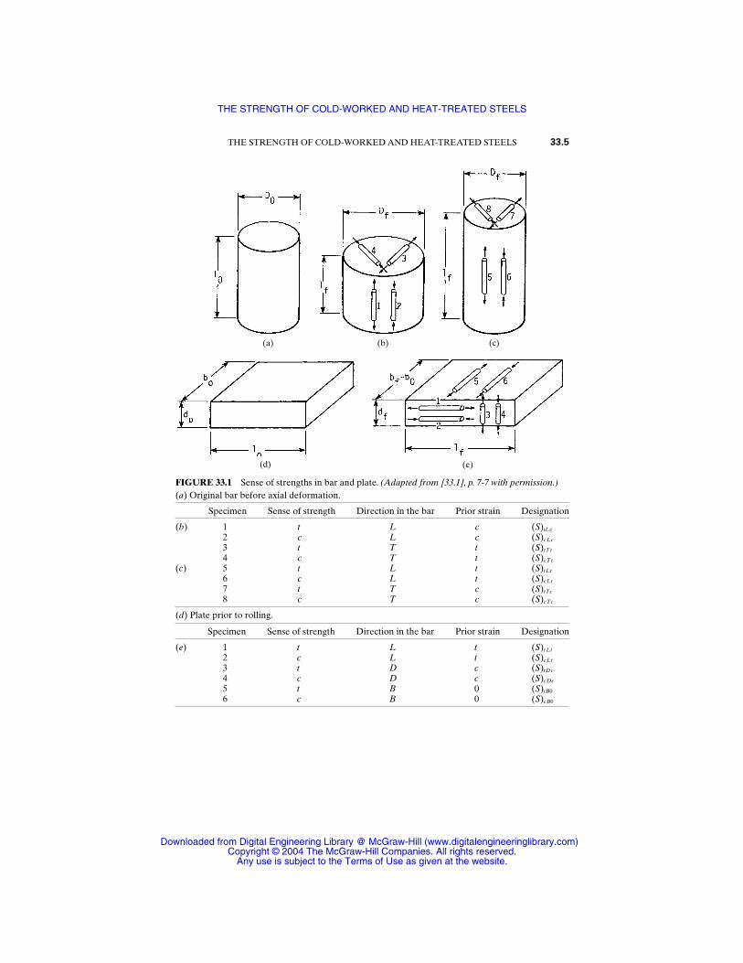
THE STRENGTH OF COLD-WORKED AND HEAT-TREATED STEELS 33.5
FIGURE 33.1 Sense of strengths in bar and plate. (Adapted from [33.1], p. 7-7 with permission.)(a) Original bar before axial deformation.
Specimen Sense of strength Direction in the bar Prior strain Designation
(b) 1 t L c (S)tLc
2 c L c (S)cLc
3 t T t (S)tT t
4 c T t (S)cT t
(c) 5 t L t (S)tLt
6 c L t (S)cLt
7 t T c (S)tTc
8 c T c (S)cTc
(d) Plate prior to rolling.
Specimen Sense of strength Direction in the bar Prior strain Designation
(e) 1 t L t (S)t Lt
2 c L t (S)cLt
3 t D c (S)tDc
4 c D c (S)cDc
5 t B 0 (S)tB0
6 c B 0 (S)cB0
(a) (b)
(d) (e)
(c)
THE STRENGTH OF COLD-WORKED AND HEAT-TREATED STEELS
Downloaded from Digital Engineering Library @ McGraw-Hill (www.digitalengineeringlibrary.com)Copyright © 2004 The McGraw-Hill Companies. All rights reserved.
Any use is subject to the Terms of Use as given at the website.
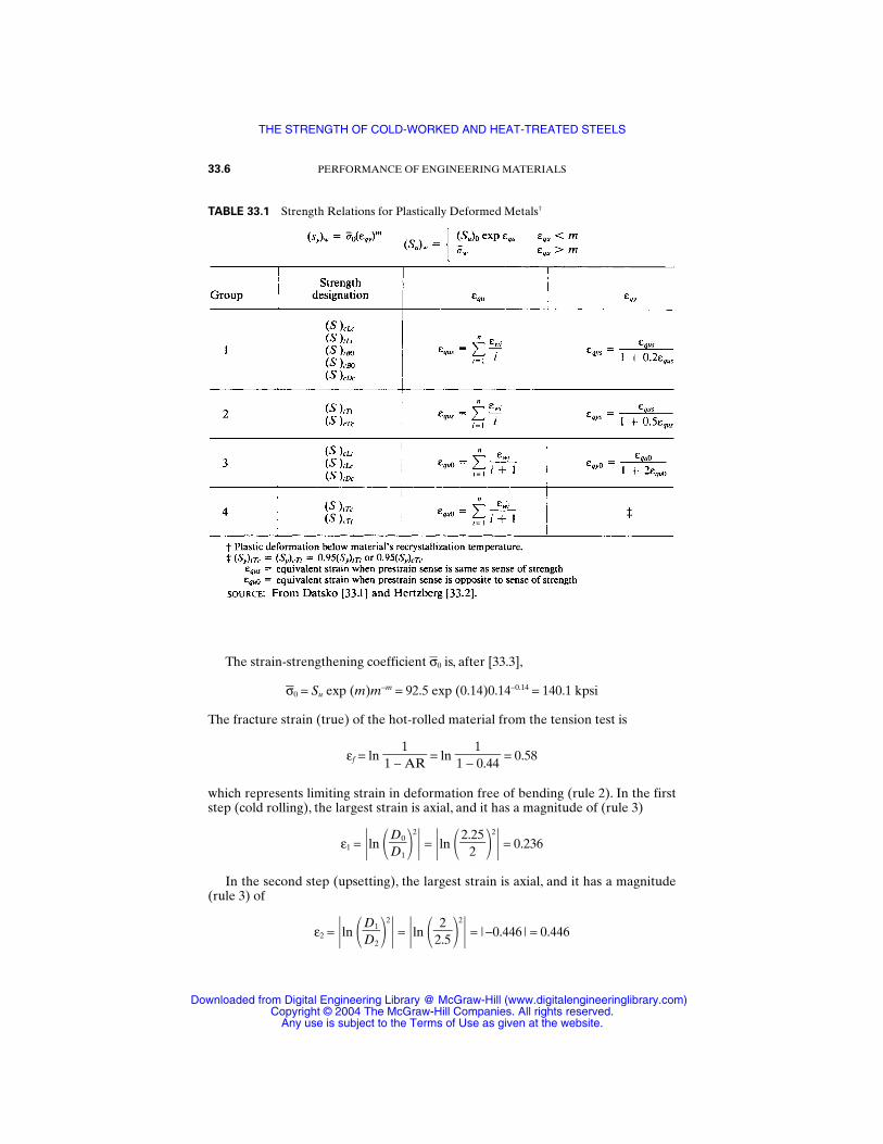
The strain-strengthening coefficient σ0 is, after [33.3],
σ0 = Su exp (m)m−m = 92.5 exp (0.14)0.14−0.14 = 140.1 kpsi
The fracture strain (true) of the hot-rolled material from the tension test is
εf = ln 1 −
1AR = ln
1 −10.44 = 0.58
which represents limiting strain in deformation free of bending (rule 2). In the firststep (cold rolling), the largest strain is axial, and it has a magnitude of (rule 3)
ε1 = ln DD
0
1
2
= ln 2.
225
2
= 0.236
In the second step (upsetting), the largest strain is axial, and it has a magnitude(rule 3) of
ε2 = ln DD
1
2
2
= ln 22.5
2
= | −0.446 | = 0.446
33.6 PERFORMANCE OF ENGINEERING MATERIALS
TABLE 33.1 Strength Relations for Plastically Deformed Metals†
THE STRENGTH OF COLD-WORKED AND HEAT-TREATED STEELS
Downloaded from Digital Engineering Library @ McGraw-Hill (www.digitalengineeringlibrary.com)Copyright © 2004 The McGraw-Hill Companies. All rights reserved.
Any use is subject to the Terms of Use as given at the website.
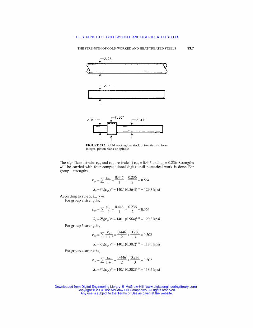
The significant strains εw1 and εw2 are (rule 4) εw1 = 0.446 and εw2 = 0.236. Strengthswill be carried with four computational digits until numerical work is done. Forgroup 1 strengths,
εqu = = 0.4
146 +
0.2236 = 0.564
Su = σ0(εqu)m = 140.1(0.564)0.14 = 129.3 kpsi
According to rule 5, εqu > m.For group 2 strengths,
εqu = = 0.4
146 +
0.2236 = 0.564
Su = σ0(εqu)m = 140.1(0.564)0.14 = 129.3 kpsi
For group 3 strengths,
εqu = = 0.4
246 +
0.2336 = 0.302
Su = σ0(εqu)m = 140.1(0.302)0.14 = 118.5 kpsi
For group 4 strengths,
εqu = = 0.4
246 +
0.2336 = 0.302
Su = σ0(εqu)m = 140.1(0.302)0.14 = 118.5 kpsi
εwi1 + i
εwi1 + i
εwii
εwii
THE STRENGTH OF COLD-WORKED AND HEAT-TREATED STEELS 33.7
FIGURE 33.2 Cold working bar stock in two steps to formintegral pinion blank on spindle.
THE STRENGTH OF COLD-WORKED AND HEAT-TREATED STEELS
Downloaded from Digital Engineering Library @ McGraw-Hill (www.digitalengineeringlibrary.com)Copyright © 2004 The McGraw-Hill Companies. All rights reserved.
Any use is subject to the Terms of Use as given at the website.
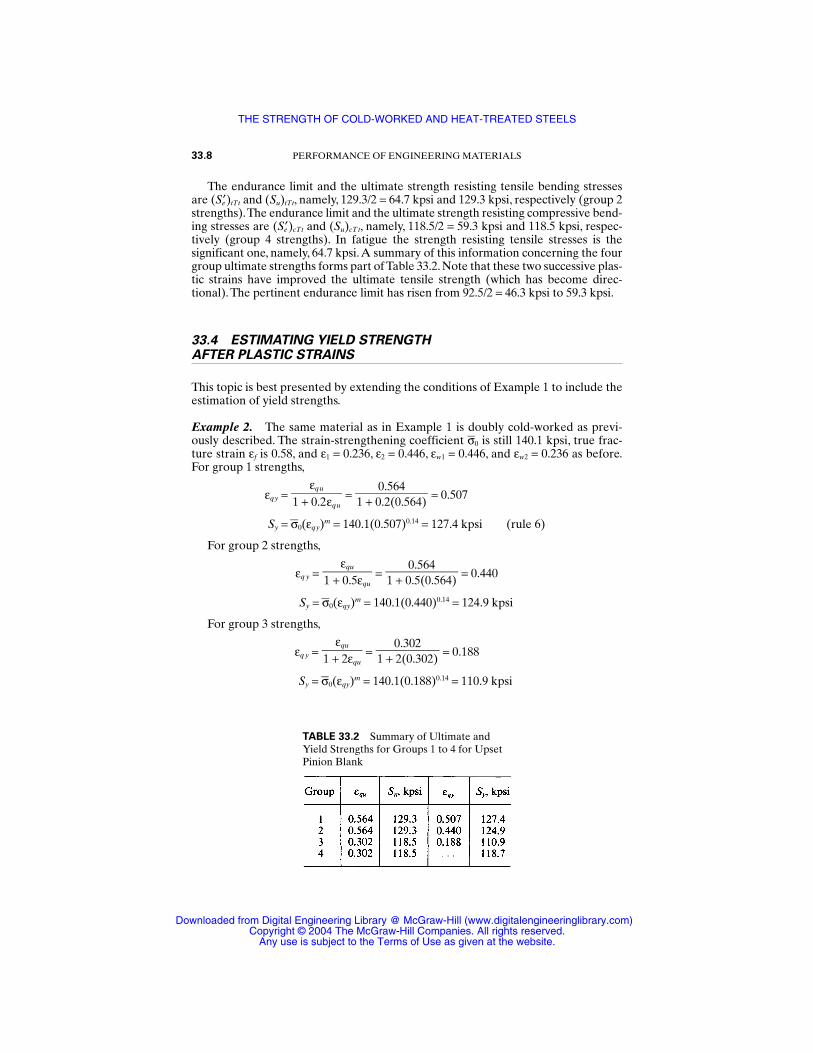
The endurance limit and the ultimate strength resisting tensile bending stressesare (Se′)tTt and (Su)tTt, namely, 129.3/2 = 64.7 kpsi and 129.3 kpsi, respectively (group 2strengths).The endurance limit and the ultimate strength resisting compressive bend-ing stresses are (Se′)cTt and (Su)cT t, namely, 118.5/2 = 59.3 kpsi and 118.5 kpsi, respec-tively (group 4 strengths). In fatigue the strength resisting tensile stresses is thesignificant one, namely, 64.7 kpsi.A summary of this information concerning the fourgroup ultimate strengths forms part of Table 33.2. Note that these two successive plas-tic strains have improved the ultimate tensile strength (which has become direc-tional). The pertinent endurance limit has risen from 92.5/2 = 46.3 kpsi to 59.3 kpsi.
33.4 ESTIMATING YIELD STRENGTH AFTER PLASTIC STRAINS
This topic is best presented by extending the conditions of Example 1 to include theestimation of yield strengths.
Example 2. The same material as in Example 1 is doubly cold-worked as previ-ously described. The strain-strengthening coefficient σ0 is still 140.1 kpsi, true frac-ture strain εf is 0.58, and ε1 = 0.236, ε2 = 0.446, εw1 = 0.446, and εw2 = 0.236 as before.For group 1 strengths,
εqy = = = 0.507
Sy = σ0(εqy)m = 140.1(0.507)0.14 = 127.4 kpsi (rule 6)
For group 2 strengths,
εq y = = = 0.440
Sy = σ0(εqy)m = 140.1(0.440)0.14 = 124.9 kpsi
For group 3 strengths,
εq y = = = 0.188
Sy = σ0(εqy)m = 140.1(0.188)0.14 = 110.9 kpsi
0.3021 + 2(0.302)
εqu1 + 2εqu
0.5641 + 0.5(0.564)
εqu1 + 0.5εqu
0.5641 + 0.2(0.564)
εqu1 + 0.2εqu
33.8 PERFORMANCE OF ENGINEERING MATERIALS
TABLE 33.2 Summary of Ultimate andYield Strengths for Groups 1 to 4 for UpsetPinion Blank
THE STRENGTH OF COLD-WORKED AND HEAT-TREATED STEELS
Downloaded from Digital Engineering Library @ McGraw-Hill (www.digitalengineeringlibrary.com)Copyright © 2004 The McGraw-Hill Companies. All rights reserved.
Any use is subject to the Terms of Use as given at the website.
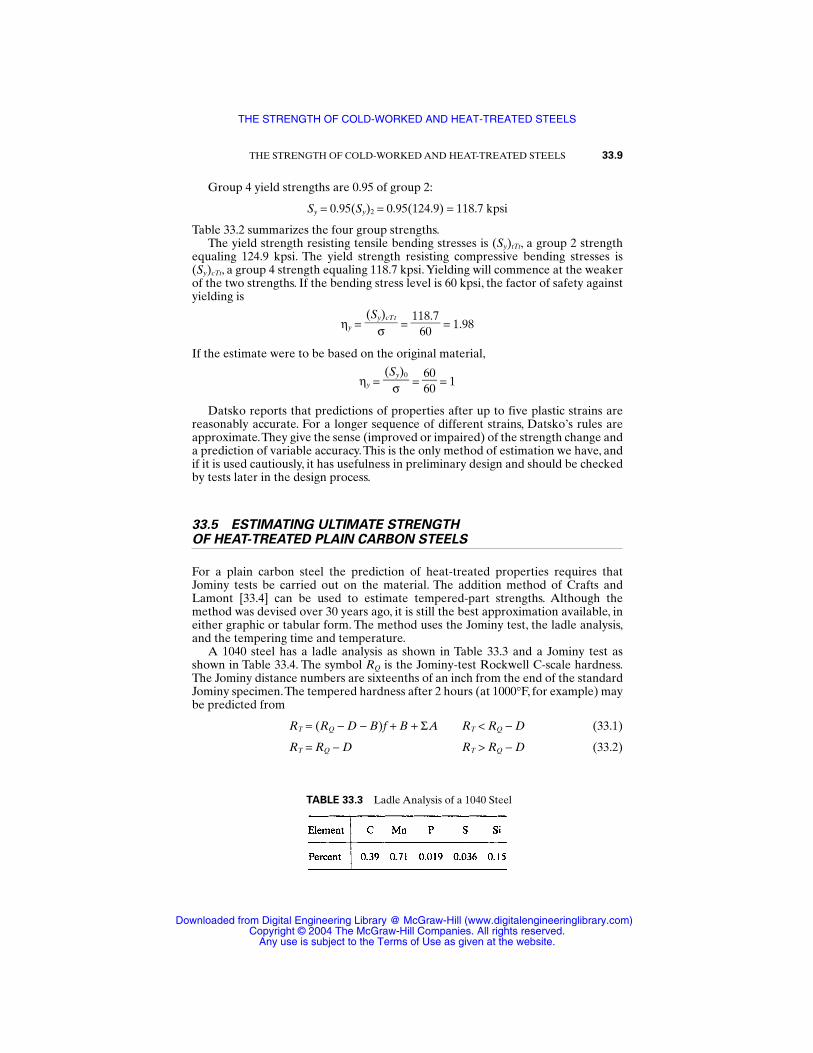
Group 4 yield strengths are 0.95 of group 2:
Sy = 0.95(Sy)2 = 0.95(124.9) = 118.7 kpsi
Table 33.2 summarizes the four group strengths.The yield strength resisting tensile bending stresses is (Sy)tTt, a group 2 strength
equaling 124.9 kpsi. The yield strength resisting compressive bending stresses is(Sy)cTt, a group 4 strength equaling 118.7 kpsi.Yielding will commence at the weakerof the two strengths. If the bending stress level is 60 kpsi, the factor of safety againstyielding is
ηy = = 11
680.7
= 1.98
If the estimate were to be based on the original material,
ηy = = 6600 = 1
Datsko reports that predictions of properties after up to five plastic strains arereasonably accurate. For a longer sequence of different strains, Datsko’s rules areapproximate.They give the sense (improved or impaired) of the strength change anda prediction of variable accuracy.This is the only method of estimation we have, andif it is used cautiously, it has usefulness in preliminary design and should be checkedby tests later in the design process.
33.5 ESTIMATING ULTIMATE STRENGTH OF HEAT-TREATED PLAIN CARBON STEELS
For a plain carbon steel the prediction of heat-treated properties requires thatJominy tests be carried out on the material. The addition method of Crafts and Lamont [33.4] can be used to estimate tempered-part strengths. Although themethod was devised over 30 years ago, it is still the best approximation available, ineither graphic or tabular form. The method uses the Jominy test, the ladle analysis,and the tempering time and temperature.
A 1040 steel has a ladle analysis as shown in Table 33.3 and a Jominy test asshown in Table 33.4. The symbol RQ is the Jominy-test Rockwell C-scale hardness.The Jominy distance numbers are sixteenths of an inch from the end of the standardJominy specimen.The tempered hardness after 2 hours (at 1000°F, for example) maybe predicted from
RT = (RQ − D − B)f + B + ΣA RT < RQ − D (33.1)
RT = RQ − D RT > RQ − D (33.2)
(Sy)0
σ
(Sy)cTt
σ
THE STRENGTH OF COLD-WORKED AND HEAT-TREATED STEELS 33.9
TABLE 33.3 Ladle Analysis of a 1040 Steel
THE STRENGTH OF COLD-WORKED AND HEAT-TREATED STEELS
Downloaded from Digital Engineering Library @ McGraw-Hill (www.digitalengineeringlibrary.com)Copyright © 2004 The McGraw-Hill Companies. All rights reserved.
Any use is subject to the Terms of Use as given at the website.
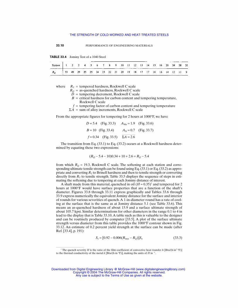
where RT = tempered hardness, Rockwell C scaleRQ = as-quenched hardness, Rockwell C scaleD = tempering decrement, Rockwell C scaleB = critical hardness for carbon content and tempering temperature,
Rockwell C scalef = tempering factor of carbon content and tempering temperature
ΣA = sum of alloy increments, Rockwell C scale
From the appropriate figures for tempering for 2 hours at 1000°F, we have
D = 5.4 (Fig. 33.3) AMn = 1.9 (Fig. 33.6)
B = 10 (Fig. 33.4) ASi = 0.7 (Fig. 33.7)
f = 0.34 (Fig. 33.5) ΣA = 2.6
The transition from Eq. (33.1) to Eq. (33.2) occurs at a Rockwell hardness deter-mined by equating these two expressions:
(RQ − 5.4 − 10)0.34 + 10 + 2.6 = RQ − 5.4
from which RQ = 19.3, Rockwell C scale. The softening at each station and corre-sponding ultimate tensile strength can be found using Eq. (33.1) or Eq. (33.2) as appro-priate and converting RT to Brinell hardness and then to tensile strength or convertingdirectly from RT to tensile strength. Table 33.5 displays the sequence of steps in esti-mating the softening due to tempering at each Jominy distance of interest.
A shaft made from this material, quenched in oil (H = 0.35)† and tempered for 2hours at 1000°F would have surface properties that are a function of the shaft’sdiameter. Figures 33.8 through 33.11 express graphically and Tables 33.6 through33.9 express numerically the equivalent Jominy distance for the surface and interiorof rounds for various severities of quench.A 1-in-diameter round has a rate of cool-ing at the surface that is the same as at Jominy distance 5.1 (see Table 33.6). Thismeans an as-quenched hardness of about 15.9 and a surface ultimate strength ofabout 105.7 kpsi. Similar determinations for other diameters in the range 0.1 to 4 inlead to the display that is Table 33.10.A table such as this is valuable to the designerand can be routinely produced by computer [33.5]. A plot of the surface ultimatestrength versus diameter from this table provides the 1000°F contour shown in Fig.33.12. An estimate of 0.2 percent yield strength at the surface can be made (afterRef. [33.4], p. 191):
Sy = [0.92 − 0.006(Rmax − RQ)]Su (33.3)
33.10 PERFORMANCE OF ENGINEERING MATERIALS
TABLE 33.4 Jominy Test of a 1040 Steel
† The quench severity H is the ratio of the film coefficient of convective heat transfer h [Btu/(h⋅in2⋅°F)]to the thermal conductivity of the metal k [Btu/(h⋅in⋅°F)], making the units of H in −1.
THE STRENGTH OF COLD-WORKED AND HEAT-TREATED STEELS
Downloaded from Digital Engineering Library @ McGraw-Hill (www.digitalengineeringlibrary.com)Copyright © 2004 The McGraw-Hill Companies. All rights reserved.
Any use is subject to the Terms of Use as given at the website.
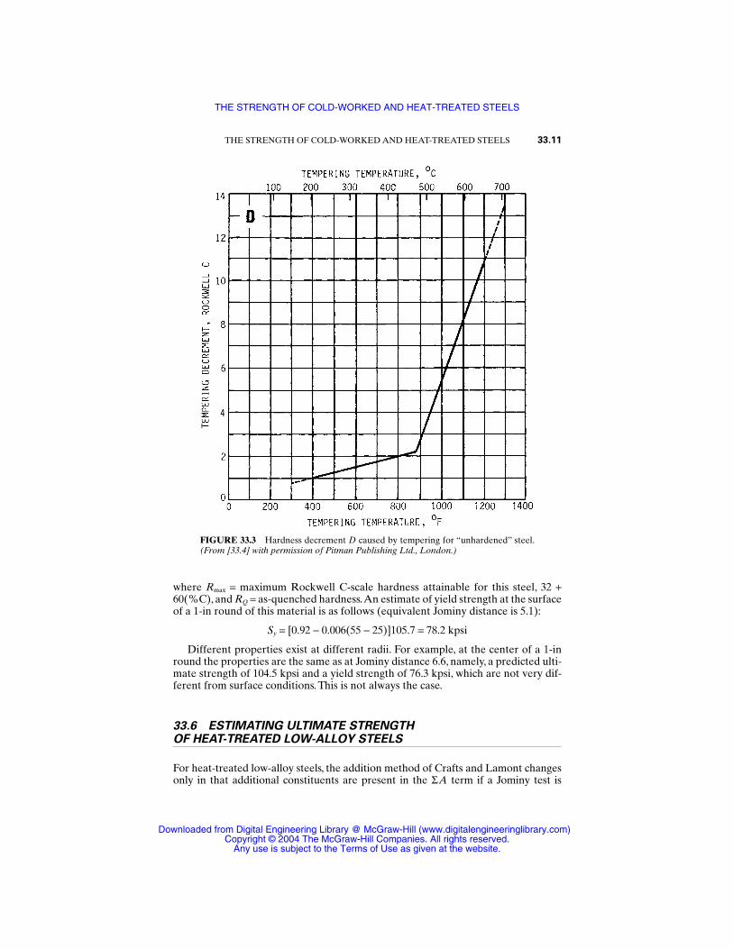
where Rmax = maximum Rockwell C-scale hardness attainable for this steel, 32 +60(%C), and RQ = as-quenched hardness.An estimate of yield strength at the surfaceof a 1-in round of this material is as follows (equivalent Jominy distance is 5.1):
Sy = [0.92 − 0.006(55 − 25)]105.7 = 78.2 kpsi
Different properties exist at different radii. For example, at the center of a 1-inround the properties are the same as at Jominy distance 6.6, namely, a predicted ulti-mate strength of 104.5 kpsi and a yield strength of 76.3 kpsi, which are not very dif-ferent from surface conditions. This is not always the case.
33.6 ESTIMATING ULTIMATE STRENGTH OF HEAT-TREATED LOW-ALLOY STEELS
For heat-treated low-alloy steels, the addition method of Crafts and Lamont changesonly in that additional constituents are present in the ΣA term if a Jominy test is
THE STRENGTH OF COLD-WORKED AND HEAT-TREATED STEELS 33.11
FIGURE 33.3 Hardness decrement D caused by tempering for “unhardened” steel.(From [33.4] with permission of Pitman Publishing Ltd., London.)
THE STRENGTH OF COLD-WORKED AND HEAT-TREATED STEELS
Downloaded from Digital Engineering Library @ McGraw-Hill (www.digitalengineeringlibrary.com)Copyright © 2004 The McGraw-Hill Companies. All rights reserved.
Any use is subject to the Terms of Use as given at the website.
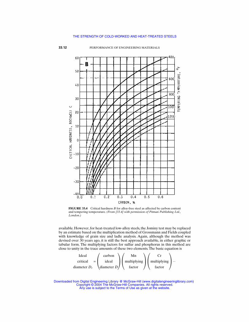
available. However, for heat-treated low-alloy steels, the Jominy test may be replacedby an estimate based on the multiplication method of Grossmann and Fields coupledwith knowledge of grain size and ladle analysis. Again, although the method wasdevised over 30 years ago, it is still the best approach available, in either graphic ortabular form. The multiplying factors for sulfur and phosphorus in this method areclose to unity in the trace amounts of these two elements. The basic equation is
Ideal carbon Mn Cr
critical = ideal multiplying multiplying ⋅⋅⋅diameter DI diameter D factor factor
33.12 PERFORMANCE OF ENGINEERING MATERIALS
FIGURE 33.4 Critical hardness B for alloy-free steel as affected by carbon contentand tempering temperature. (From [33.4] with permission of Pitman Publishing Ltd.,London.)
THE STRENGTH OF COLD-WORKED AND HEAT-TREATED STEELS
Downloaded from Digital Engineering Library @ McGraw-Hill (www.digitalengineeringlibrary.com)Copyright © 2004 The McGraw-Hill Companies. All rights reserved.
Any use is subject to the Terms of Use as given at the website.
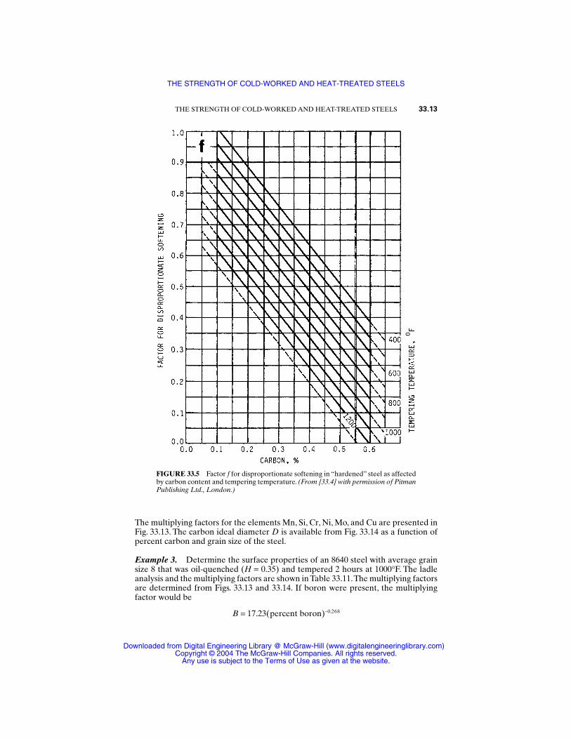
The multiplying factors for the elements Mn, Si, Cr, Ni, Mo, and Cu are presented inFig. 33.13. The carbon ideal diameter D is available from Fig. 33.14 as a function ofpercent carbon and grain size of the steel.
Example 3. Determine the surface properties of an 8640 steel with average grainsize 8 that was oil-quenched (H = 0.35) and tempered 2 hours at 1000°F. The ladleanalysis and the multiplying factors are shown in Table 33.11.The multiplying factorsare determined from Figs. 33.13 and 33.14. If boron were present, the multiplyingfactor would be
B = 17.23(percent boron)−0.268
THE STRENGTH OF COLD-WORKED AND HEAT-TREATED STEELS 33.13
FIGURE 33.5 Factor f for disproportionate softening in “hardened” steel as affectedby carbon content and tempering temperature. (From [33.4] with permission of PitmanPublishing Ltd., London.)
THE STRENGTH OF COLD-WORKED AND HEAT-TREATED STEELS
Downloaded from Digital Engineering Library @ McGraw-Hill (www.digitalengineeringlibrary.com)Copyright © 2004 The McGraw-Hill Companies. All rights reserved.
Any use is subject to the Terms of Use as given at the website.
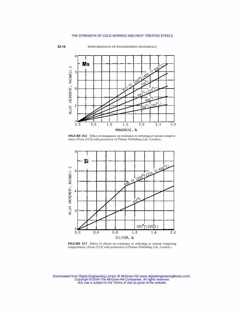
33.14 PERFORMANCE OF ENGINEERING MATERIALS
FIGURE 33.6 Effect of manganese on resistance to softening at various tempera-tures. (From [33.4] with permission of Pitman Publishing Ltd., London.)
FIGURE 33.7 Effect of silicon on resistance to softening at various temperingtemperatures. (From [33.4] with permission of Pitman Publishing Ltd., London.)
THE STRENGTH OF COLD-WORKED AND HEAT-TREATED STEELS
Downloaded from Digital Engineering Library @ McGraw-Hill (www.digitalengineeringlibrary.com)Copyright © 2004 The McGraw-Hill Companies. All rights reserved.
Any use is subject to the Terms of Use as given at the website.
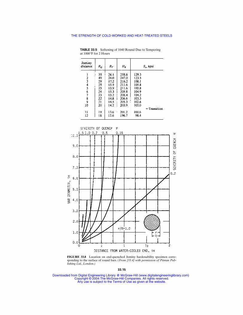
TABLE 33.5 Softening of 1040 Round Due to Temperingat 1000°F for 2 Hours
FIGURE 33.8 Location on end-quenched Jominy hardenability specimen corre-sponding to the surface of round bars. (From [33.4] with permission of Pitman Pub-lishing Ltd., London.)
33.15
THE STRENGTH OF COLD-WORKED AND HEAT-TREATED STEELS
Downloaded from Digital Engineering Library @ McGraw-Hill (www.digitalengineeringlibrary.com)Copyright © 2004 The McGraw-Hill Companies. All rights reserved.
Any use is subject to the Terms of Use as given at the website.
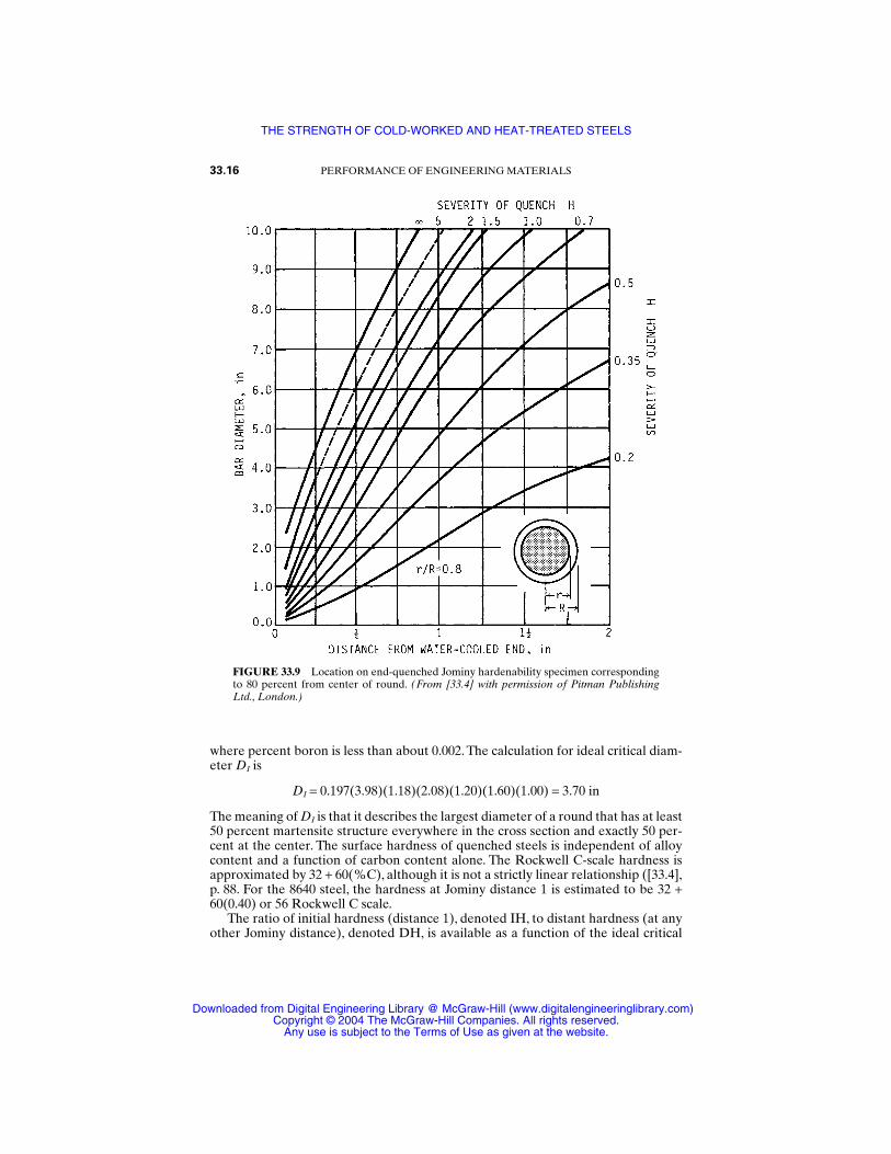
where percent boron is less than about 0.002. The calculation for ideal critical diam-eter DI is
DI = 0.197(3.98)(1.18)(2.08)(1.20)(1.60)(1.00) = 3.70 in
The meaning of DI is that it describes the largest diameter of a round that has at least50 percent martensite structure everywhere in the cross section and exactly 50 per-cent at the center. The surface hardness of quenched steels is independent of alloycontent and a function of carbon content alone. The Rockwell C-scale hardness isapproximated by 32 + 60(%C), although it is not a strictly linear relationship ([33.4],p. 88. For the 8640 steel, the hardness at Jominy distance 1 is estimated to be 32 +60(0.40) or 56 Rockwell C scale.
The ratio of initial hardness (distance 1), denoted IH, to distant hardness (at anyother Jominy distance), denoted DH, is available as a function of the ideal critical
33.16 PERFORMANCE OF ENGINEERING MATERIALS
FIGURE 33.9 Location on end-quenched Jominy hardenability specimen correspondingto 80 percent from center of round. (From [33.4] with permission of Pitman PublishingLtd., London.)
THE STRENGTH OF COLD-WORKED AND HEAT-TREATED STEELS
Downloaded from Digital Engineering Library @ McGraw-Hill (www.digitalengineeringlibrary.com)Copyright © 2004 The McGraw-Hill Companies. All rights reserved.
Any use is subject to the Terms of Use as given at the website.
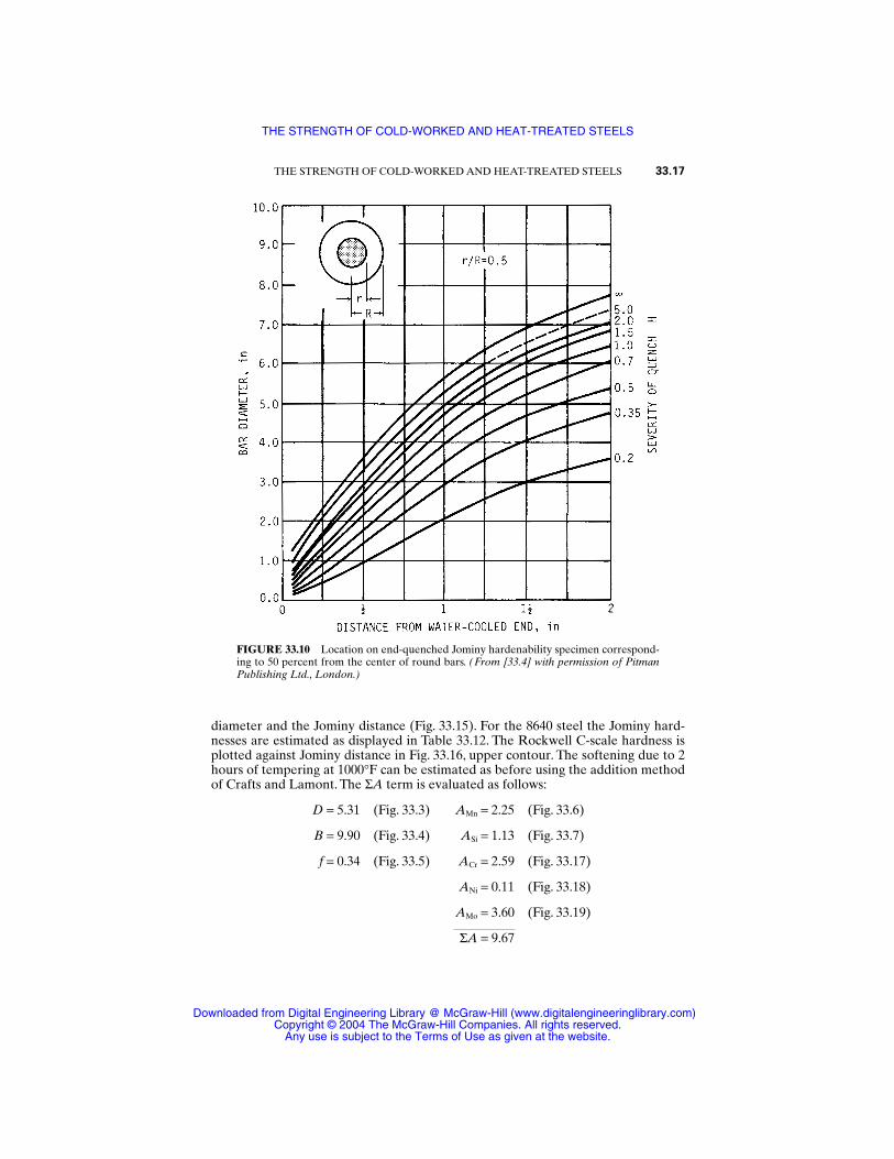
diameter and the Jominy distance (Fig. 33.15). For the 8640 steel the Jominy hard-nesses are estimated as displayed in Table 33.12. The Rockwell C-scale hardness isplotted against Jominy distance in Fig. 33.16, upper contour. The softening due to 2hours of tempering at 1000°F can be estimated as before using the addition methodof Crafts and Lamont. The ΣA term is evaluated as follows:
D = 5.31 (Fig. 33.3) AMn = 2.25 (Fig. 33.6)
B = 9.90 (Fig. 33.4) ASi = 1.13 (Fig. 33.7)
f = 0.34 (Fig. 33.5) ACr = 2.59 (Fig. 33.17)
ANi = 0.11 (Fig. 33.18)
AMo = 3.60 (Fig. 33.19)
ΣA = 9.67
THE STRENGTH OF COLD-WORKED AND HEAT-TREATED STEELS 33.17
FIGURE 33.10 Location on end-quenched Jominy hardenability specimen correspond-ing to 50 percent from the center of round bars. (From [33.4] with permission of PitmanPublishing Ltd., London.)
THE STRENGTH OF COLD-WORKED AND HEAT-TREATED STEELS
Downloaded from Digital Engineering Library @ McGraw-Hill (www.digitalengineeringlibrary.com)Copyright © 2004 The McGraw-Hill Companies. All rights reserved.
Any use is subject to the Terms of Use as given at the website.
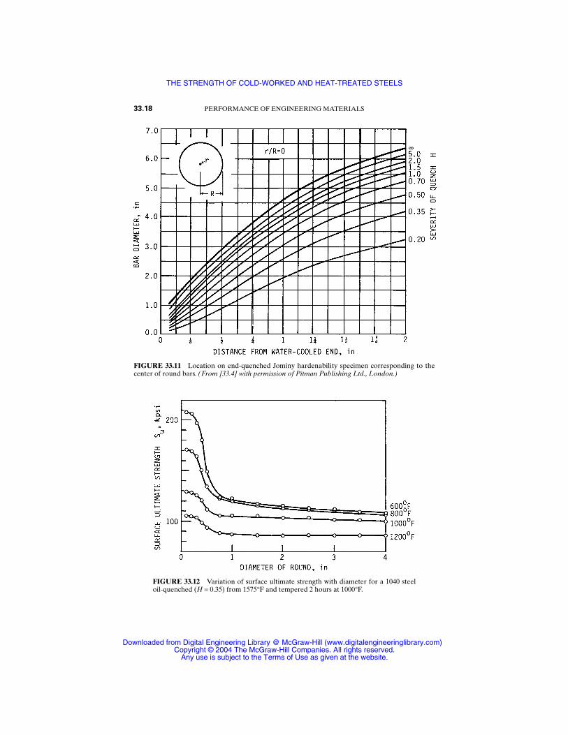
33.18 PERFORMANCE OF ENGINEERING MATERIALS
FIGURE 33.11 Location on end-quenched Jominy hardenability specimen corresponding to thecenter of round bars. (From [33.4] with permission of Pitman Publishing Ltd., London.)
FIGURE 33.12 Variation of surface ultimate strength with diameter for a 1040 steeloil-quenched (H = 0.35) from 1575°F and tempered 2 hours at 1000°F.
THE STRENGTH OF COLD-WORKED AND HEAT-TREATED STEELS
Downloaded from Digital Engineering Library @ McGraw-Hill (www.digitalengineeringlibrary.com)Copyright © 2004 The McGraw-Hill Companies. All rights reserved.
Any use is subject to the Terms of Use as given at the website.
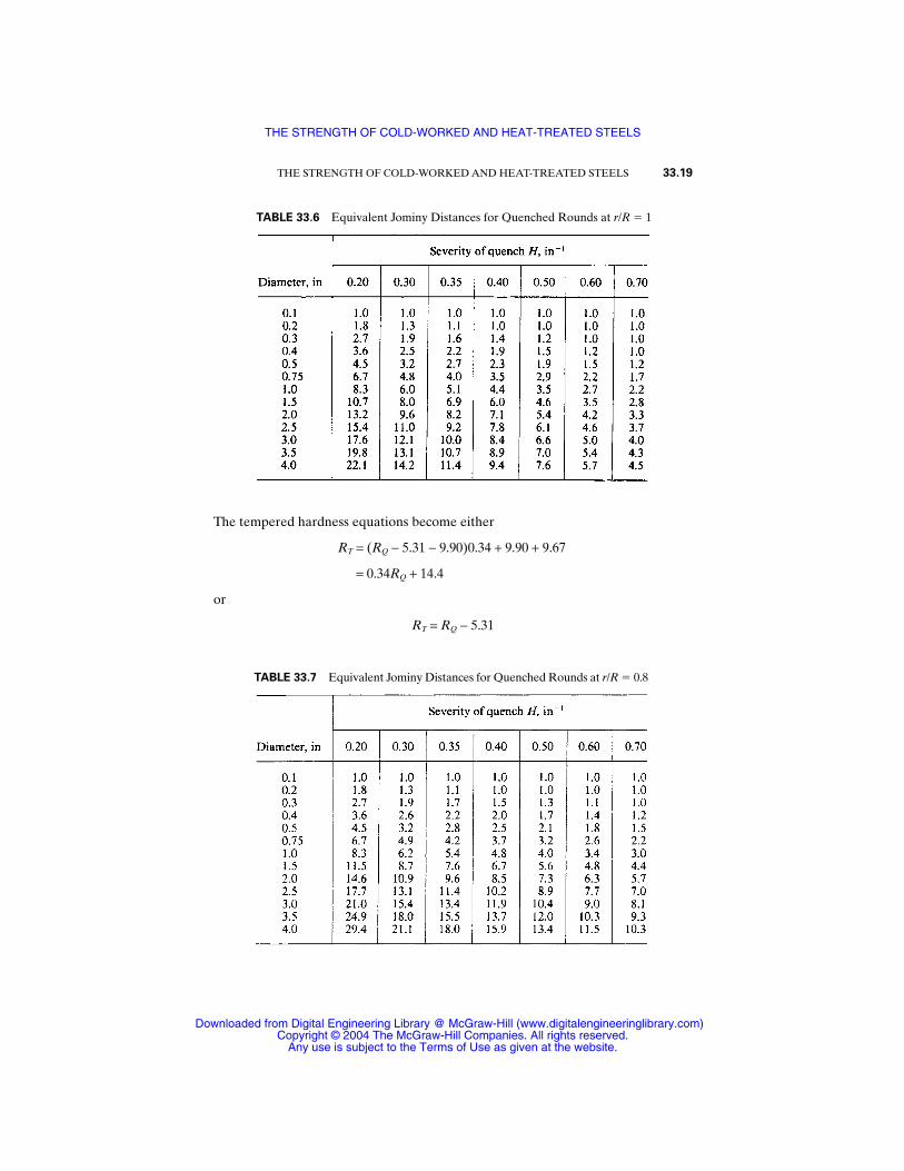
The tempered hardness equations become either
RT = (RQ − 5.31 − 9.90)0.34 + 9.90 + 9.67
= 0.34RQ + 14.4
or
RT = RQ − 5.31
THE STRENGTH OF COLD-WORKED AND HEAT-TREATED STEELS 33.19
TABLE 33.6 Equivalent Jominy Distances for Quenched Rounds at r/R 1
TABLE 33.7 Equivalent Jominy Distances for Quenched Rounds at r/R 0.8
THE STRENGTH OF COLD-WORKED AND HEAT-TREATED STEELS
Downloaded from Digital Engineering Library @ McGraw-Hill (www.digitalengineeringlibrary.com)Copyright © 2004 The McGraw-Hill Companies. All rights reserved.
Any use is subject to the Terms of Use as given at the website.
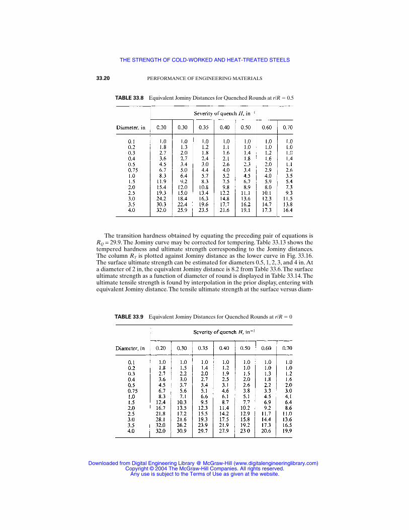
The transition hardness obtained by equating the preceding pair of equations isRQ = 29.9. The Jominy curve may be corrected for tempering. Table 33.13 shows thetempered hardness and ultimate strength corresponding to the Jominy distances.The column RT is plotted against Jominy distance as the lower curve in Fig. 33.16.The surface ultimate strength can be estimated for diameters 0.5, 1, 2, 3, and 4 in. Ata diameter of 2 in, the equivalent Jominy distance is 8.2 from Table 33.6.The surfaceultimate strength as a function of diameter of round is displayed in Table 33.14. Theultimate tensile strength is found by interpolation in the prior display, entering withequivalent Jominy distance.The tensile ultimate strength at the surface versus diam-
33.20 PERFORMANCE OF ENGINEERING MATERIALS
TABLE 33.8 Equivalent Jominy Distances for Quenched Rounds at r/R 0.5
TABLE 33.9 Equivalent Jominy Distances for Quenched Rounds at r/R 0
THE STRENGTH OF COLD-WORKED AND HEAT-TREATED STEELS
Downloaded from Digital Engineering Library @ McGraw-Hill (www.digitalengineeringlibrary.com)Copyright © 2004 The McGraw-Hill Companies. All rights reserved.
Any use is subject to the Terms of Use as given at the website.
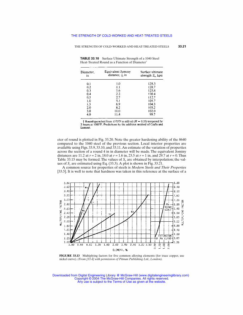
eter of round is plotted in Fig. 33.20. Note the greater hardening ability of the 8640compared to the 1040 steel of the previous section. Local interior properties areavailable using Figs. 33.9, 33.10, and 33.11.An estimate of the variation of propertiesacross the section of a round 4 in in diameter will be made. The equivalent Jominydistances are 11.2 at r = 2 in, 18.0 at r = 1.6 in, 23.5 at r = 1 in, and 29.7 at r = 0. ThusTable 33.15 may be formed. The values of Su are obtained by interpolation; the val-ues of Sy are estimated using Eq. (33.3). A plot is shown in Fig. 33.21.
A common source for properties of steels is Modern Steels and Their Properties[33.5]. It is well to note that hardness was taken in this reference at the surface of a
THE STRENGTH OF COLD-WORKED AND HEAT-TREATED STEELS 33.21
TABLE 33.10 Surface Ultimate Strength of a 1040 SteelHeat-Treated Round as a Function of Diameter†
FIGURE 33.13 Multiplying factors for five common alloying elements (for trace copper, usenickel curve). (From [33.4] with permission of Pitman Publishing Ltd., London).
THE STRENGTH OF COLD-WORKED AND HEAT-TREATED STEELS
Downloaded from Digital Engineering Library @ McGraw-Hill (www.digitalengineeringlibrary.com)Copyright © 2004 The McGraw-Hill Companies. All rights reserved.
Any use is subject to the Terms of Use as given at the website.
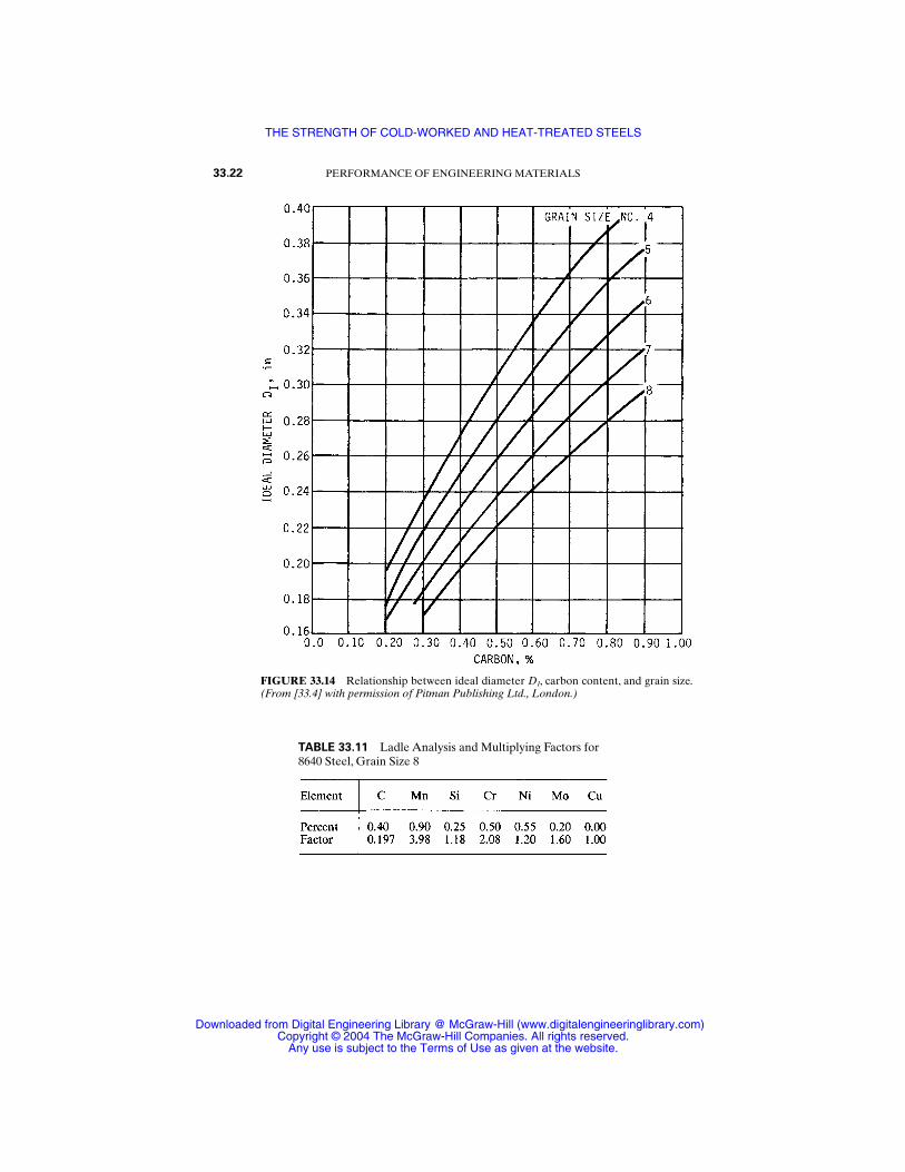
33.22 PERFORMANCE OF ENGINEERING MATERIALS
FIGURE 33.14 Relationship between ideal diameter DI, carbon content, and grain size.(From [33.4] with permission of Pitman Publishing Ltd., London.)
TABLE 33.11 Ladle Analysis and Multiplying Factors for8640 Steel, Grain Size 8
THE STRENGTH OF COLD-WORKED AND HEAT-TREATED STEELS
Downloaded from Digital Engineering Library @ McGraw-Hill (www.digitalengineeringlibrary.com)Copyright © 2004 The McGraw-Hill Companies. All rights reserved.
Any use is subject to the Terms of Use as given at the website.
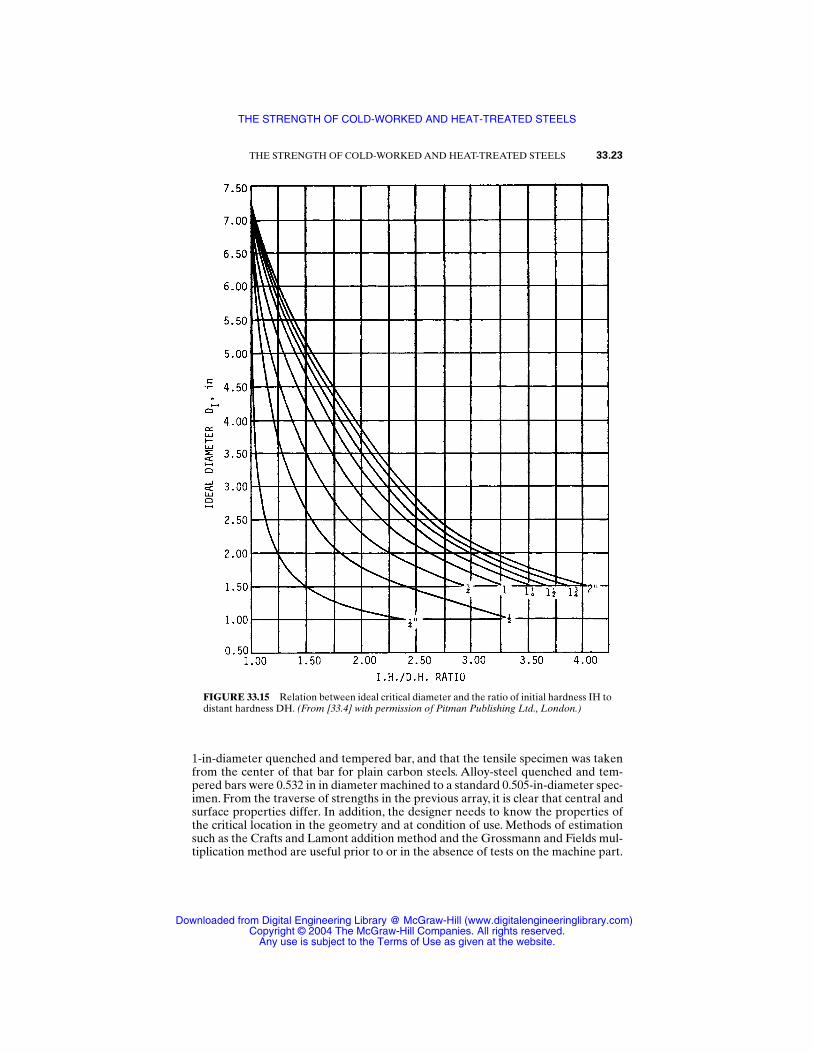
1-in-diameter quenched and tempered bar, and that the tensile specimen was takenfrom the center of that bar for plain carbon steels. Alloy-steel quenched and tem-pered bars were 0.532 in in diameter machined to a standard 0.505-in-diameter spec-imen. From the traverse of strengths in the previous array, it is clear that central andsurface properties differ. In addition, the designer needs to know the properties ofthe critical location in the geometry and at condition of use. Methods of estimationsuch as the Crafts and Lamont addition method and the Grossmann and Fields mul-tiplication method are useful prior to or in the absence of tests on the machine part.
THE STRENGTH OF COLD-WORKED AND HEAT-TREATED STEELS 33.23
FIGURE 33.15 Relation between ideal critical diameter and the ratio of initial hardness IH todistant hardness DH. (From [33.4] with permission of Pitman Publishing Ltd., London.)
THE STRENGTH OF COLD-WORKED AND HEAT-TREATED STEELS
Downloaded from Digital Engineering Library @ McGraw-Hill (www.digitalengineeringlibrary.com)Copyright © 2004 The McGraw-Hill Companies. All rights reserved.
Any use is subject to the Terms of Use as given at the website.

These methods have produced for a 4-in round of 8640, quenched in oil (H = 0.35)from 1575°F, and tempered for 2 hours at 1000°F, the property estimates displayedas Table 33.16. Reference [33.6] is a circular slide rule implementation of the multi-plication method of Grossmann and Fields.
Current efforts are directed toward refining the information rather than displac-ing the ideas upon which Secs. 33.5 and 33.6 are based ([33.7], [33.8]). Probabilisticelements of the predicted Jominy curve are addressed in Ho [33.9].
33.24 PERFORMANCE OF ENGINEERING MATERIALS
FIGURE 33.16 Predicted Jominy signature for a 8640 steel with softening pro-duced by 2-hour tempering at 1000°F.
TABLE 33.12 Prediction of Jominy Curvefor 8640 Steel by Multiplication Method ofGrossmann and Fields
THE STRENGTH OF COLD-WORKED AND HEAT-TREATED STEELS
Downloaded from Digital Engineering Library @ McGraw-Hill (www.digitalengineeringlibrary.com)Copyright © 2004 The McGraw-Hill Companies. All rights reserved.
Any use is subject to the Terms of Use as given at the website.
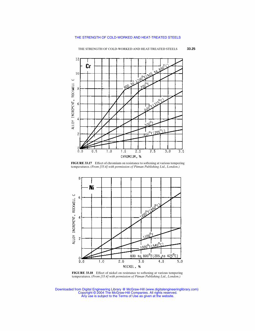
THE STRENGTH OF COLD-WORKED AND HEAT-TREATED STEELS 33.25
FIGURE 33.17 Effect of chromium on resistance to softening at various temperingtemperatures. (From [33.4] with permission of Pitman Publishing Ltd., London.)
FIGURE 33.18 Effect of nickel on resistance to softening at various temperingtemperatures. (From [33.4] with permission of Pitman Publishing Ltd., London.)
THE STRENGTH OF COLD-WORKED AND HEAT-TREATED STEELS
Downloaded from Digital Engineering Library @ McGraw-Hill (www.digitalengineeringlibrary.com)Copyright © 2004 The McGraw-Hill Companies. All rights reserved.
Any use is subject to the Terms of Use as given at the website.
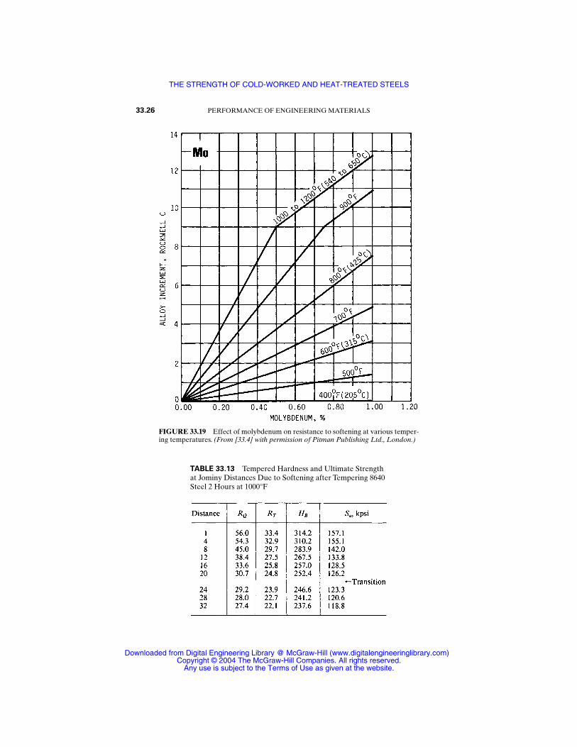
33.26 PERFORMANCE OF ENGINEERING MATERIALS
FIGURE 33.19 Effect of molybdenum on resistance to softening at various temper-ing temperatures. (From [33.4] with permission of Pitman Publishing Ltd., London.)
TABLE 33.13 Tempered Hardness and Ultimate Strengthat Jominy Distances Due to Softening after Tempering 8640Steel 2 Hours at 1000°F
THE STRENGTH OF COLD-WORKED AND HEAT-TREATED STEELS
Downloaded from Digital Engineering Library @ McGraw-Hill (www.digitalengineeringlibrary.com)Copyright © 2004 The McGraw-Hill Companies. All rights reserved.
Any use is subject to the Terms of Use as given at the website.
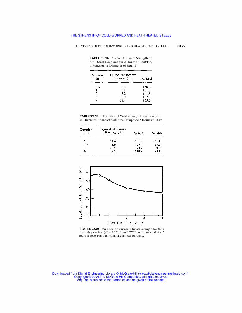
THE STRENGTH OF COLD-WORKED AND HEAT-TREATED STEELS 33.27
TABLE 33.14 Surface Ultimate Strength of8640 Steel Tempered for 2 Hours at 1000°F asa Function of Diameter of Round
TABLE 33.15 Ultimate and Yield Strength Traverse of a 4-in-Diameter Round of 8640 Steel Tempered 2 Hours at 1000º
FIGURE 33.20 Variation on surface ultimate strength for 8640steel oil-quenched (H = 0.35) from 1575°F and tempered for 2hours at 1000°F as a function of diameter of round.
THE STRENGTH OF COLD-WORKED AND HEAT-TREATED STEELS
Downloaded from Digital Engineering Library @ McGraw-Hill (www.digitalengineeringlibrary.com)Copyright © 2004 The McGraw-Hill Companies. All rights reserved.
Any use is subject to the Terms of Use as given at the website.
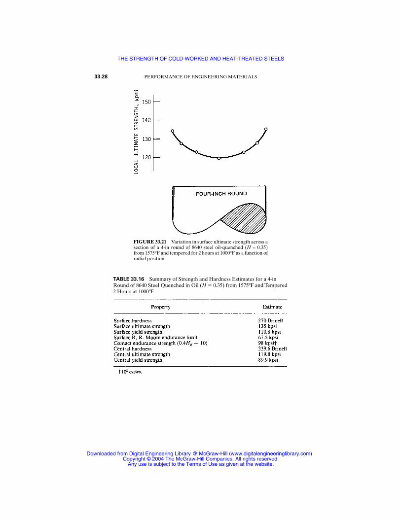
33.28 PERFORMANCE OF ENGINEERING MATERIALS
FIGURE 33.21 Variation in surface ultimate strength across asection of a 4-in round of 8640 steel oil-quenched (H = 0.35)from 1575°F and tempered for 2 hours at 1000°F as a function ofradial position.
TABLE 33.16 Summary of Strength and Hardness Estimates for a 4-inRound of 8640 Steel Quenched in Oil (H 0.35) from 1575ºF and Tempered2 Hours at 1000ºF
THE STRENGTH OF COLD-WORKED AND HEAT-TREATED STEELS
Downloaded from Digital Engineering Library @ McGraw-Hill (www.digitalengineeringlibrary.com)Copyright © 2004 The McGraw-Hill Companies. All rights reserved.
Any use is subject to the Terms of Use as given at the website.
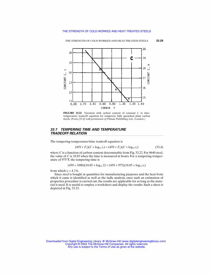
33.7 TEMPERING TIME AND TEMPERATURETRADEOFF RELATION
The tempering-temperature/time tradeoff equation is
(459 + F1)(C + log10 t1) = (459 + F2)(C + log10 t2) (33.4)
where C is a function of carbon content determinable from Fig. 33.22. For 8640 steel,the value of C is 18.85 when the time is measured in hours. For a tempering temper-ature of 975°F, the tempering time is
(459 + 1000)(18.85 + log10 2) = (459 + 975)(18.85 + log10 t2)
from which t2 = 4.3 h.Since steel is bought in quantities for manufacturing purposes and the heat from
which it came is identified as well as the ladle analysis, once such an estimation ofproperties procedure is carried out, the results are applicable for as long as the mate-rial is used. It is useful to employ a worksheet and display the results. Such a sheet isdepicted in Fig. 33.23.
THE STRENGTH OF COLD-WORKED AND HEAT-TREATED STEELS 33.29
FIGURE 33.22 Variation with carbon content of constant C in time-temperature tradeoff equation for tempered, fully quenched plain carbonsteels. (From [33.4] with permission of Pitman Publishing Ltd., London.)
THE STRENGTH OF COLD-WORKED AND HEAT-TREATED STEELS
Downloaded from Digital Engineering Library @ McGraw-Hill (www.digitalengineeringlibrary.com)Copyright © 2004 The McGraw-Hill Companies. All rights reserved.
Any use is subject to the Terms of Use as given at the website.
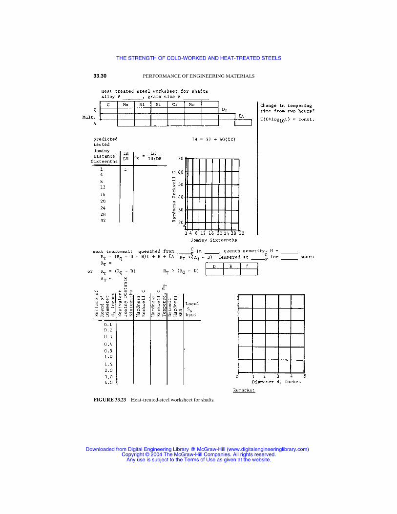
33.30 PERFORMANCE OF ENGINEERING MATERIALS
FIGURE 33.23 Heat-treated-steel worksheet for shafts.
THE STRENGTH OF COLD-WORKED AND HEAT-TREATED STEELS
Downloaded from Digital Engineering Library @ McGraw-Hill (www.digitalengineeringlibrary.com)Copyright © 2004 The McGraw-Hill Companies. All rights reserved.
Any use is subject to the Terms of Use as given at the website.

REFERENCES
33.1 J. Datsko, Materials in Design and Manufacturing, published by the author, Ann Arbor,Mich., 1977.
33.2 M. P. Borden, “Multidimensional Tensile Properties of Materials Subjected to LargeCyclic Strains,” Ph.D. thesis, University of Michigan, Ann Arbor, 1975.
33.3 R. W. Hertzberg, Deformation and Fracture Mechanics of Engineering Materials, JohnWiley & Sons, New York, 1976.
33.4 W. Crafts and J. L. Lamont, Hardenability and Steel Selection, Pitman & Sons, London,1949.
33.5 Modern Steels and Their Properties, Bethlehem Steel Corporation, 1972.
33.6 Bethlehem Alloy Steel Hardenability Calculator, Calc 96, Bethlehem Steel Corpora-tion, 1966.
33.7 D. V. Doane and J. J. Kirkaldy (eds.), Hardenability Concepts with Applications to Steel,American Institute of Mining, Metallurgical and Petroleum Engineers, Warrendale,Pa., 1978.
33.8 C. A. Siebert, D. V. Doane, and D. H. Breen, The Hardenability of Steels, American Soci-ety for Metals, Metals Park, Ohio, 1977.
33.9 T. K. Ho, “Probabilistic Prediction of the Jominy Curve of Low Alloy Steels from Com-position and Grain Size,” Ph.D. thesis, Iowa State University, Ames, 1978.
RECOMMENDED READING
C. S. Brady and H. R. Clauser, Metals Handbook, 11th ed., McGraw-Hill, New York, 1977.E. A. Brandes (ed.), Smithells Metal Reference Book, 6th ed., Butterworths, London, 1983.C. R. Brooks, Heat Treatment, Structure and Properties of Non Ferrous Alloys, American Soci-
ety for Metals, Metals Park, Ohio, 1982.P. Harvey (ed.), Engineering Properties of Steel, American Society for Metals, Metals Park,
Ohio, 1982.G. Krauss, Principles of Heat Treatment of Steel, American Society for Metals, Metals Park,
Ohio, 1980.Metals Handbook, 9th ed., Vol. 1: Properties and Selection: Irons and Steels; Vol. 4: Heat Treat-
ing, American Society for Metals, Metals Park, Ohio, 1981.
THE STRENGTH OF COLD-WORKED AND HEAT-TREATED STEELS 33.31
THE STRENGTH OF COLD-WORKED AND HEAT-TREATED STEELS
Downloaded from Digital Engineering Library @ McGraw-Hill (www.digitalengineeringlibrary.com)Copyright © 2004 The McGraw-Hill Companies. All rights reserved.
Any use is subject to the Terms of Use as given at the website.

THE STRENGTH OF COLD-WORKED AND HEAT-TREATED STEELS
Downloaded from Digital Engineering Library @ McGraw-Hill (www.digitalengineeringlibrary.com)Copyright © 2004 The McGraw-Hill Companies. All rights reserved.
Any use is subject to the Terms of Use as given at the website.
CHAPTER 34WEAR
Kenneth C. LudemaProfessor of Mechanical Engineering
Department of Mechanical Engineering and Applied MechanicsThe University of Michigan
Ann Arbor, Michigan
34.1 GENERAL PRINCIPLES IN DESIGN FOR WEAR RESISTANCE / 34.1
34.2 STEPS IN DESIGN FOR WEAR LIFE WITHOUT SELECTING MATERIALS / 34.4
34.3 WEAR EQUATIONS / 34.6
34.4 STEPS IN SELECTING MATERIALS FOR WEAR RESISTANCE / 34.7
34.5 MATERIAL-SELECTION PROCEDURE / 34.14
REFERENCES / 34.18
BIBLIOGRAPHY / 34.18
There is no shorthand method of designing machinery for a specified wear life.Thusa step-by-step method is given for designers to follow. The method begins with anexamination of worn parts of the type to be improved. The next step is an estimateof stresses, temperatures, and likely conditions of operation of the redesignedmachinery. Material testing for wear resistance is discussed, and finally, a procedureis given for selecting materials for wear resistance.
34.1 GENERAL PRINCIPLES IN DESIGN FOR WEAR RESISTANCE
The wear life of mechanical components is affected by nearly as many variables ashuman life. Wearing surfaces are composed of substrate material, oxide, absorbedgas, and dirt. They respond to their environment, method of manufacture, and con-ditions of operation. They suffer acute and/or progressive degeneration, and theycan often be partially rehabilitated by either a change in operating conditions orsome intrusive action.
The range of wearing components and devices is endless, including animal teethand joints, cams, piston rings, tires, roads, brakes, dirt seals, liquid seals, gas seals,belts, floors, shoes, fabrics, electrical contacts, disks and tapes, tape heads, printerheads, tractor tracks, cannon barrels, rolling mills, dies, sheet products, forgings, orecrushers, conveyors, nuclear machinery, home appliances, sleeve bearings, rolling-element bearings, door hinges, zippers, drills, saws, razor blades, pump impellers,valve seats, pipe bends, stirring paddles, plastic molding screws and dies, and erasers.There is not a single universal approach to designing all these components for anacceptable wear life, but there are some rational design steps for some.There are no
34.1
Source: STANDARD HANDBOOK OF MACHINE DESIGN
Downloaded from Digital Engineering Library @ McGraw-Hill (www.digitalengineeringlibrary.com)Copyright © 2004 The McGraw-Hill Companies. All rights reserved.
Any use is subject to the Terms of Use as given at the website.
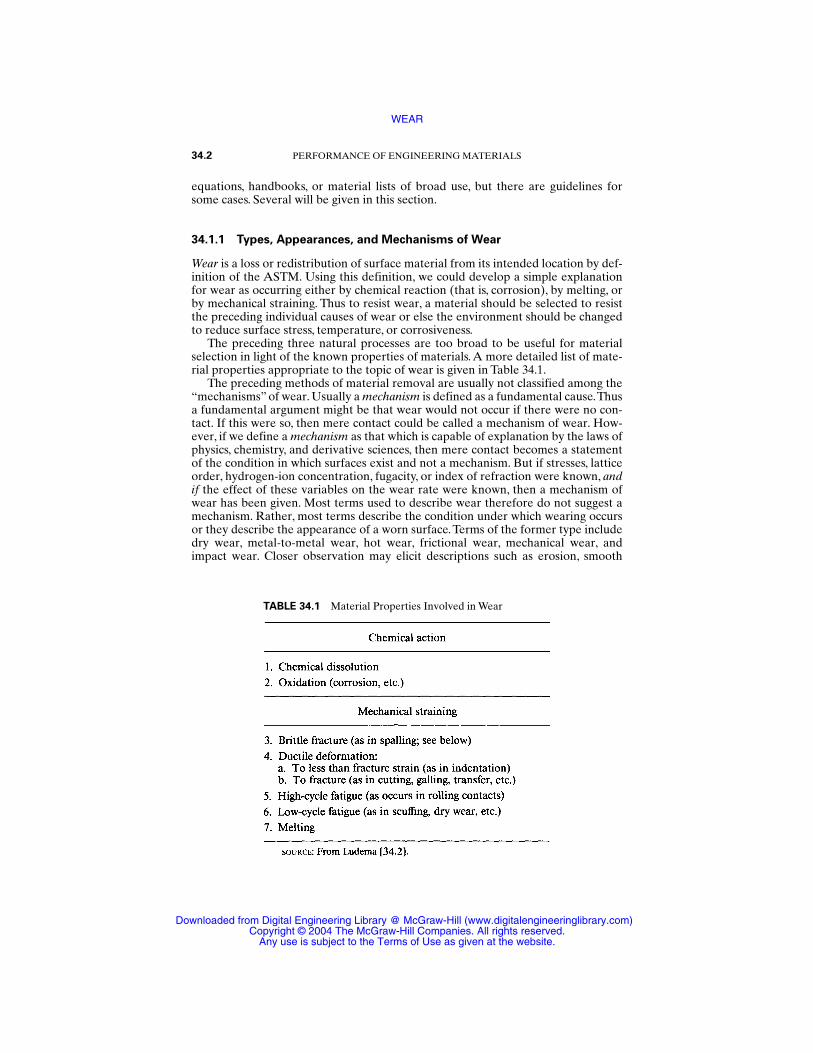
equations, handbooks, or material lists of broad use, but there are guidelines forsome cases. Several will be given in this section.
34.1.1 Types, Appearances, and Mechanisms of Wear
Wear is a loss or redistribution of surface material from its intended location by def-inition of the ASTM. Using this definition, we could develop a simple explanationfor wear as occurring either by chemical reaction (that is, corrosion), by melting, orby mechanical straining. Thus to resist wear, a material should be selected to resistthe preceding individual causes of wear or else the environment should be changedto reduce surface stress, temperature, or corrosiveness.
The preceding three natural processes are too broad to be useful for materialselection in light of the known properties of materials. A more detailed list of mate-rial properties appropriate to the topic of wear is given in Table 34.1.
The preceding methods of material removal are usually not classified among the“mechanisms” of wear. Usually a mechanism is defined as a fundamental cause.Thusa fundamental argument might be that wear would not occur if there were no con-tact. If this were so, then mere contact could be called a mechanism of wear. How-ever, if we define a mechanism as that which is capable of explanation by the laws ofphysics, chemistry, and derivative sciences, then mere contact becomes a statementof the condition in which surfaces exist and not a mechanism. But if stresses, latticeorder, hydrogen-ion concentration, fugacity, or index of refraction were known, andif the effect of these variables on the wear rate were known, then a mechanism ofwear has been given. Most terms used to describe wear therefore do not suggest amechanism. Rather, most terms describe the condition under which wearing occursor they describe the appearance of a worn surface. Terms of the former type includedry wear, metal-to-metal wear, hot wear, frictional wear, mechanical wear, andimpact wear. Closer observation may elicit descriptions such as erosion, smooth
34.2 PERFORMANCE OF ENGINEERING MATERIALS
TABLE 34.1 Material Properties Involved in Wear
WEAR
Downloaded from Digital Engineering Library @ McGraw-Hill (www.digitalengineeringlibrary.com)Copyright © 2004 The McGraw-Hill Companies. All rights reserved.
Any use is subject to the Terms of Use as given at the website.
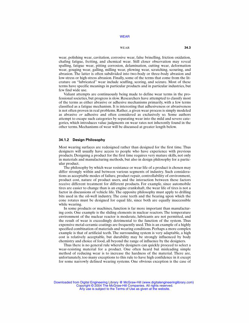
wear, polishing wear, cavitation, corrosive wear, false brinelling, friction oxidation,chafing fatigue, fretting, and chemical wear. Still closer observation may revealspalling, fatigue wear, pitting corrosion, delamination, cutting wear, deformationwear, gouging wear, galling, milling wear, plowing wear, scratching, scouring, andabrasion. The latter is often subdivided into two-body or three-body abrasion andlow-stress or high-stress abrasion. Finally, some of the terms that come from the lit-erature on “lubricated” wear include scuffing, scoring, and seizure. Most of theseterms have specific meanings in particular products and in particular industries, butfew find wide use.
Valiant attempts are continuously being made to define wear terms in the pro-fessional societies, but progress is slow. Researchers have attempted to classify mostof the terms as either abrasive or adhesive mechanisms primarily, with a few termsclassified as a fatigue mechanism. It is interesting that adhesiveness or abrasivenessis not often proven in real problems. Rather, a given wear process is simply modeledas abrasive or adhesive and often considered as exclusively so. Some authorsattempt to escape such categories by separating wear into the mild and severe cate-gories, which introduces value judgments on wear rates not inherently found in theother terms. Mechanisms of wear will be discussed at greater length below.
34.1.2 Design Philosophy
Most wearing surfaces are redesigned rather than designed for the first time. Thusdesigners will usually have access to people who have experience with previousproducts. Designing a product for the first time requires very mature skills, not onlyin materials and manufacturing methods, but also in design philosophy for a partic-ular product.
The philosophy by which wear resistance or wear life of a product is chosen maydiffer strongly within and between various segments of industry. Such considera-tions as acceptable modes of failure, product repair, controllability of environment,product cost, nature of product users, and the interaction between these factorsreceive different treatment for different products. For example, since automobiletires are easier to change than is an engine crankshaft, the wear life of tires is not afactor in discussions of vehicle life. The opposite philosophy must apply to drillingbits used in the oil-well industry. The cone teeth and the bearing upon which thecone rotates must be designed for equal life, since both are equally inaccessiblewhile wearing.
In some products or machines, function is far more important than manufactur-ing costs. One example is the sliding elements in nuclear reactors. The temperatureenvironment of the nuclear reactor is moderate, lubricants are not permitted, andthe result of wear is exceedingly detrimental to the function of the system. Thusexpensive metal-ceramic coatings are frequently used.This is an example of a highlyspecified combination of materials and wearing conditions. Perhaps a more complexexample is that of artificial teeth. The surrounding system is very adaptable, a highcost is relatively acceptable, but durability may be strongly influenced by bodychemistry and choice of food, all beyond the range of influence by the designers.
Thus there is no general rule whereby designers can quickly proceed to select awear-resisting material for a product. One often heard but misleading simplemethod of reducing wear is to increase the hardness of the material. There are,unfortunately, too many exceptions to this rule to have high confidence in it exceptfor some narrowly defined wearing systems. One obvious exception is the case of
WEAR 34.3
WEAR
Downloaded from Digital Engineering Library @ McGraw-Hill (www.digitalengineeringlibrary.com)Copyright © 2004 The McGraw-Hill Companies. All rights reserved.
Any use is subject to the Terms of Use as given at the website.
bronzes, which are more successful as a gear material against a hardened-steel pin-ion than is a hardened-steel gear.The reason usually given for the success of bronzeis that dirt particles are readily embedded into the bronze and therefore do not cutor wear the steel away, but this is more of an intuitive argument than fact. Anotherexception to the hardness rule is the cams in automotive engines. They are hard-ened in the range of 50 Rockwell C instead of to the maximum available, which maybe as high as 67 RC.A final example is that of buckets and chutes for handling someores. Rubber is sometimes found to be superior to very hard white cast iron in theseapplications.
We see in the preceding examples the possibility of special circumstancesrequiring special materials. The rubber offers resilience, and the cam materialresists fatigue failure if it is not fully hardened. It is often argued that special cir-cumstances are rare or can be dealt with on a case-by-case basis. This attitudeseems to imply that most wearing systems are “standard,” thus giving impetus tospecifying a basic wear resistance of a material as one of its intrinsic properties.Little real progress has been made in this effort, and very little is likely to be madein the near future. Wear resistance is achieved by a balance of several very sepa-rate properties, not all of them intrinsic, that are different for each machine com-ponent or wear surface. Selecting material for wear resistance is therefore acomplex task, and guidelines are needed in design. Such guidelines will be moreuseful as our technology becomes more complex, but some guidelines are given inthe next section.
34.2 STEPS IN DESIGN FOR WEAR LIFE WITHOUT SELECTING MATERIALS
34.2.1 The Search for Standard Components
Designers make most of the decisions concerning material selection. Fortunately,for many cases and for most designers, the crucial components in a machine inwhich wear may limit useful machine life are available as separate packages withfairly well specified performance capabilities. Examples are gear boxes, clutches,and bearings. Most such components have been well tested in the marketplace, hav-ing been designed and developed by very experienced designers. For componentdesigners, very general rules for selecting materials are of little value. They mustbuild devices with a predicted wear life of ±10 percent accuracy or better. Theyknow the range of capability of lubricants, they know the reasonable range of tem-perature in which their products will survive, and they know how to classify shockloads and other real operating conditions.Their specific expertise is not available tothe general designer except in the form of the shapes and dimensions of hardware,the materials selected, and the recommended practices for use of their product.Some of these selections are based on tradition, and some are based on reasoning,strongly tempered by experience. The makers of specialized components usuallyalso have the facilities to test new designs and materials extensively before riskingtheir product in real use. General designers, however, must often proceed withoutextensive testing.
General designers must then decide whether to avail themselves of standard spe-cialized components or to risk designing every part. Sometimes the choice is basedon economics, and sometimes desired standard components are not available. Insuch cases, components as well as other machine parts must be designed in-house.
34.4 PERFORMANCE OF ENGINEERING MATERIALS
WEAR
Downloaded from Digital Engineering Library @ McGraw-Hill (www.digitalengineeringlibrary.com)Copyright © 2004 The McGraw-Hill Companies. All rights reserved.
Any use is subject to the Terms of Use as given at the website.
34.2.2 In-House Design
If a designer is required to design for wear resistance, it is logical to follow the meth-ods used in parallel activities, such as in determining the strength and vibration characteristics of new machinery. This is often done by interpolating within orextrapolating beyond experience, if any, using
1. Company practice for similar items2. Vendors of materials, lubricants, and components3. Handbooks
Company Practice. If good information is available on similar items, a predictionof the wear life of a new product can be made with ± 20 percent accuracy unless theoperating conditions of the new design are much beyond standard experience. Sim-ple scaling of sizes and loads is often successful, but usually this technique fails aftera few iterations. Careless comparison of a new design with “similar” existing itemscan produce very large errors for reasons discussed below.
When a new product must be designed that involves loads, stresses, or speedsbeyond those previously experienced, it is often helpful to examine the worn surfaceof a well-used previous model in detail. It is also helpful to examine unsuccessfulprototypes or wear-test specimens, as will be discussed below.An assessment shouldbe made of the modes or mechanisms of wear of each part of the product. For thispurpose, it is also useful to examine old lubricants, the contents of the lubricantsump, and other accumulations of residue.
Vendors of Materials. Where a new product requires bearings or materials ofhigher capacity than now in use, it is frequently helpful to contact vendors of suchproducts. When a vendor simply suggests an existing item or material, the wear lifeof a new product may not be predictable to an accuracy of better than ± 50 percentof the desired life. This accuracy is worse than the ± 20 percent accuracy given ear-lier, especially where there is inadequate communication between the designer andthe vendor. Accuracy may be improved where an interested vendor carefullyassesses the needs of a design, supplies a sample for testing, and follows the designactivity to the end.
Contact with vendors, incidentally, often has a general beneficial effect. It encour-ages designers to revise their thinking beyond the logical projection of their ownexperience. Most designers need a steady flow of information from vendors toremain informed on both the new products and the changing capability of products.
Handbooks. There are very few handbooks on selecting materials for wear resis-tance. Materials and design handbooks usually provide lists of materials, some ofwhich are highlighted as having been successfully used in wearing parts of variousproducts. They usually provide little information on the rates of wear of products,the mode of wear failure, the limits on operating conditions, or the method by whichthe wear-resisting parts should be manufactured or run in (if necessary).
Some sources will give wear coefficients, which are purported to be figures ofmerit, or rank placing of materials for wear resistance. A major limitation of wearcoefficients of materials as given in most literature is that there is seldom adequateinformation given on how the data were obtained. Usually this information is takenfrom standard laboratory bench tests, few of which simulate real systems. The finalresult of the use of handbook data is a design which will probably not perform to anaccuracy of better than ±95 percent.
WEAR 34.5
WEAR
Downloaded from Digital Engineering Library @ McGraw-Hill (www.digitalengineeringlibrary.com)Copyright © 2004 The McGraw-Hill Companies. All rights reserved.
Any use is subject to the Terms of Use as given at the website.
34.3 WEAR EQUATIONS
There is a great need for wear equations. Ideally, a wear equation would provide anumerical value for material loss or transfer for a wide range of materials and oper-ating conditions of the wearing parts.
Useful equations derived from fundamental principles are not yet available.Some empirical equations are available for very special conditions. The strictlyempirical equations usually contain very few variables and are of the form
VTn = f adbK (34.1)
which applies to metal cutting, and in which V = cutting speed, T = tool life, f = feedrate, and d = depth of cut. Experiments are done, measuring T over a range of f whileholding V and d fixed at some arbitrary values, from which a can be obtained. Theexperiments are repeated over ranges of d and V to obtain b and K. It is generallyassumed that the results will not depend on the selection of the variables to holdconstant, which therefore assumes that there is neither any limit to the range of validvariables nor any interdependence between variables, which ultimately means thatthere is no change of wearing mechanisms over any chosen range of the variables.Wear equations built by strictly empirical methods are therefore seen to be limitedto the case under present study; they have limited ability to predict conditionsbeyond those of the tests from which they were derived, and they have little appli-cability to other sliding systems.
A common method of building equations from fundamental principles is toassume that wearing will take place in direct proportion to the real (microscopic)contact area. These equations omit such important considerations as the presence ofoxides and adsorbed gases on surfaces, and few of them recognize the role ofrepeated contact on sliding surfaces, which may lead to fatigue modes of material loss(wear).
In a recent study [34.1], over 180 wear equations were analyzed as to content andform. Though the authors collectively cited over 100 variables to use in these equa-tions, few authors cited more than 5. The fact, then, that quantities such as hardnessare found in the numerator of some equations and in the denominator of othersleads to some confusion. Overall, no way was found to harmonize any selected groupof equations, nor was there any way to determine which material properties areimportant to the wearing properties.
The parameters that may be included in the equation are of three types, as listedin Table 34.2. It may be readily seen from Table 34.2 that many of the parameters aredifficult to quantify, and yet these (and perhaps several more) are known to affectthe wear rate. Further complexity is added in cases where wear mechanisms, andtherefore wear rates, change with time of sliding.
This state of affairs seems incomprehensible to designers who are steeped inmathematical methods that promise precise results. To use a specific example: Forcalculating the deflections of beams, simple equations are available that require onlyone material property, namely, Young’s modulus. All other quantities in these equa-tions are very specific; that is, they are measured in dimensions which not only seemavailable in four or five significant figures, but have compatible units.
Wear is far more complex, involving up to seven basic mechanisms that are oper-ative in different balances or ratios under various conditions. Moreover, many of themechanisms produce wear rates that are not linear in the simple parameters, such asapplied load, sliding speed, surface finish, etc.Thus, in summary, there are at this time
34.6 PERFORMANCE OF ENGINEERING MATERIALS
WEAR
Downloaded from Digital Engineering Library @ McGraw-Hill (www.digitalengineeringlibrary.com)Copyright © 2004 The McGraw-Hill Companies. All rights reserved.
Any use is subject to the Terms of Use as given at the website.

no complete first principles or models available to use in selecting materials for wearresistance. However, there are good procedures to follow in selecting materials forwear resistance.
34.4 STEPS IN SELECTING MATERIALS FOR WEAR RESISTANCE
When designing for wear resistance, it is necessary to ascertain that wear will pro-ceed by the same mechanism throughout the substantial portion of the life of theproduct. Only then is some reasonable prediction of life possible.
WEAR 34.7
TABLE 34.2 Parameters Often Seen in Wear Equations
WEAR
Downloaded from Digital Engineering Library @ McGraw-Hill (www.digitalengineeringlibrary.com)Copyright © 2004 The McGraw-Hill Companies. All rights reserved.
Any use is subject to the Terms of Use as given at the website.
Certain considerations are vital in selecting materials, and these may be moreimportant than selecting a material for the best wear resistance. These considera-tions are
1. The restriction on material use2. Whether the sliding surface can withstand the expected static load3. Whether the materials can withstand the sliding severity4. Whether a break-in procedure is necessary or prohibited5. The acceptable modes of wear failure or surface damage6. The possibility of testing candidate materials in bench tests or in prototype
machines
These considerations are discussed in detail in the next several pages.
34.4.1 Restrictions on Material Use
The first step in selecting materials for wear resistance is to determine whether thereare any restrictions on material use. In some industries it is necessary for economicand other purposes to use, for example, a gray cast iron, or a material that is com-patible with the human body, or a material with no cobalt in it such as is required ina nuclear reactor, or a material with high friction, or a selected surface treatmentapplied to a low-cost substrate. Furthermore, there may be a limitation on the sur-face finish available or the skill of the personnel to manufacture or assemble theproduct. Finally, there may be considerations of delivery or storage of the itembefore use, leading to corrosion, or false brinelling, or several other events that maybefall a wear surface.
34.4.2 Static Load
The second step is to determine whether the sliding surface can withstand theexpected static load without indentation or excessive distortion. Generally, thiswould involve a simple stress analysis.
34.4.3 Sliding Severity
The materials used must be able to withstand the severity of sliding. Factors involvedin determining sliding severity include the contact pressure or stress, the tempera-ture due to ambient heating and frictional temperature rise, the sliding speed, mis-alignment, duty cycle, and type of maintenance the designed item will receive.Thesefactors are explained as follows.
Contact Stress. Industrial standards for allowable contact pressure vary consid-erably. Some specifications in the gear and sleeve bearing industries limit the aver-age contact pressures for bronzes to about 1.7 MPa, which is about 1 to 4 percentof the yield strength of bronze. Likewise, in pump parts and valves made of toolsteel, the contact pressures are limited to about 140 MPa, which is about 4 to 6 per-cent of the yield strength of the hardest state of tool steel.
34.8 PERFORMANCE OF ENGINEERING MATERIALS
WEAR
Downloaded from Digital Engineering Library @ McGraw-Hill (www.digitalengineeringlibrary.com)Copyright © 2004 The McGraw-Hill Companies. All rights reserved.
Any use is subject to the Terms of Use as given at the website.
However, one example of high contact pressure is the sleeve bearings in thelanding gear of modern commercial aircraft. These materials again are bronzesand have yield strengths up to 760 MPa. The design bearing stress is 415 MPa butwith expectations of peak stressing up to 620 MPa. Another example is the use oftool steel in lubricated sheet-metal drawing. Dies may be expected to be used for500 000 parts with contact pressures of about 860 MPa, which is half the yieldstrength.
Temperature. The life of some sliding systems is strongly influenced by tempera-ture. Handbooks often specify a material for “wear” conditions without stating arange of temperature within which the wear-resistance behavior is satisfactory. Theinfluence of temperature may be its effect on the mechanical properties of the slid-ing parts. High temperatures soften most materials and low temperatures embrittlesome. High temperature will produce degradation of most lubricants, but low tem-perature will solidify a liquid lubricant.
Ambient temperature is often easy to measure, but the temperature rise due tosliding may have a larger influence. For a quick view of the factors that influencetemperature rise ∆T of asperities on rubbing surfaces, we may reproduce one simpleequation:
∆T = (34.2)
where f = coefficient of friction, W = applied load, V = sliding speed, and k1 and k2 =thermal conductivities of the sliding materials. The quantity a is related to junctionsize, that is, the few, widely scattered points of contact between sliding parts.
From Eq. (34.2) it may seem that thermal conductivity of the materials could beinfluential in controlling temperature rise in some cases, but a more important fac-tor is f, the coefficient of friction. If a temperature-sensitive wear mechanism isoperative in a particular case, then high friction may contribute to a high wear rate,if not cause it. There is at least a quantitative connection between wear rate and thecoefficient of friction when one compares dry sliding with adequately lubricatedsliding, but there is no formal way to connect the coefficient of friction with the tem-perature rise.
Sliding Speed. Both the sliding speed and the PV limits are involved in deter-mining the sliding severity. Maximum allowable loads and sliding speeds for mate-rials are often specified in catalogs in the form of PV limits. In the PV product, Pis the calculated average contact pressure (in psi) and V is the sliding speed (inft/min). Plastics to be used in sleeve bearings and bronze bushings are the mostcommon material to have PV limits assigned to them. A common range of PV lim-its for plastics is from 500 to 10 000, and these data are usually taken from simplelaboratory test devices. The quantity P is calculated from W/A, where W = appliedload and A = projected load-carrying area between sliding members. Thus PVcould be written as WV/A. Returning to Eq. (34.2) for the temperature rise, it maybe seen that the product WV influences ∆T directly, and it would seem that a PVlimit might essentially be a limit on surface-temperature rise.This is approximatelytrue, but not useful. That is, wear resistance of materials cannot be related in a sim-ple way to the melting point or softening temperature of materials. The wideranges of f, k, and other properties of materials prevent formulating a general ruleon the relationship between PV limits and melting temperature. Indeed, a PV limitindicates nothing about the actual rate of wear of materials; it indicates only that
fW V2a(k1 + k2)J
WEAR 34.9
WEAR
Downloaded from Digital Engineering Library @ McGraw-Hill (www.digitalengineeringlibrary.com)Copyright © 2004 The McGraw-Hill Companies. All rights reserved.
Any use is subject to the Terms of Use as given at the website.
above a given PV limit a very severe form of wear may occur. However, the PVlimit for one material has meaning relative to that of other materials, at least intest machinery.
Misalignment. The difficulty with misalignment is that it is an undefined conditionother than that for which contact pressure between two surfaces is usually calcu-lated. Where some misalignment may exist, it is best to use materials that can adjustor accommodate themselves, that is, break in properly.
Misalignment arises from manufacturing errors or from a deflection of the system-producing loading at one edge of the bearing, or it may arise from thermaldistortion of the system, etc. Thus a designer must consider designing a system suchthat a load acts at the expected location in a bearing under all conditions. This mayinvolve designing a flexible bearing mount, or several bearings along the length of ashaft, or a distribution of the applied loading, etc.
Designers must also consider the method of assembly of a device. A perfectlymanufactured set of parts can be inappropriately or improperly assembled, produc-ing misalignment or distortion. A simple tapping of a ball bearing with a hammer toseat the race may constitute more severe service than occurs in the lifetime of themachine and often results in early failure.
Misalignment may result from wear. If abrasive species can enter a bearing, thefastest wear will occur at the point of entry of the dirt. In that region, the bearing willwear away and transfer the load to other locations.A successful design must accountfor such events.
Duty Cycle. Important factors in selecting materials for wear resistance are theextent of shock loading of sliding systems, stop-start operations, oscillatory opera-tion, etc. It is often useful to determine also what materials surround the sliding sys-tem, such as chemical or abrasive particles.
Maintenance. A major consideration that may be classified under sliding sever-ity is maintenance. Whereas most phosphor bronze bushings are allowed a contactstress of about 1.4 to 7 MPa, aircraft wheel bushings made of beryllium bronze areallowed a maximum stress of 620 MPa, as mentioned before. The beryllium bronzehas a strength only twice that of the phosphor bronze, but the difference betweenindustrial and aircraft use includes different treatment of bearings in maintenance.Industrial goals are to place an object into service and virtually ignore it or provideinfrequently scheduled maintenance. Aircraft maintenance, however, is more rig-orous, and each operating part is under regular scrutiny by the flight crew andground crew. There is scheduled maintenance, but there is also careful continuousobservation of the part and supplies. Thus it is easier for an error to be made inselection of the lubricant in industry than with aircraft, for example. Second, theaircraft wheel bearing operates in a much more standard or narrowly defined envi-ronment. Industrial machinery must operate in the dirtiest and hottest of placesand with the poorest care. These must be considered as severity conditions by thedesigner.
34.4.4 Break-In Procedure
Another vital consideration in the selection of materials is to determine whether ornot a break-in procedure is necessary or prohibited. It cannot be assumed that the
34.10 PERFORMANCE OF ENGINEERING MATERIALS
WEAR
Downloaded from Digital Engineering Library @ McGraw-Hill (www.digitalengineeringlibrary.com)Copyright © 2004 The McGraw-Hill Companies. All rights reserved.
Any use is subject to the Terms of Use as given at the website.
sliding surfaces made to a dimensional accuracy and specified surface finish areready for service. Sliding alters surfaces. Frequently, sliding under controlled lightloads can prepare a surface for a long life of high loading, whereas immediate oper-ation at moderate loads may cause early failure.
It is useful here to distinguish between two surface-altering strategies. The firstwe refer to as break-in, where a system is immediately loaded or operated to itsdesign load. The incidence of failure of a population of such parts decreases withtime of operation as the sliding surfaces change, and frequently the ability of the sys-tem to accommodate an overload or inadequate lubricant increases in the sametime. The surfaces have changed in some way during running, and this is break-in.Run-in, however, is the deliberate and planned action that is necessary to preparesurfaces for normal service.
The wear that occurs during run-in or break-in can be considered a final modifi-cation to the machine surface. This leads to the possibility that a more careful speci-fication of manufacturing practice may obviate the need for run-in or break-in. Thishas been the case with the automobile engine in particular, although part of a suc-cessful part surface-finish specification often includes the exact technique for mak-ing the surface. Only 30 years ago it was necessary to start and run an enginecarefully for the first few thousand miles to ensure a reasonable engine life. If run-inwere necessary today, one would not see an engine survive the short trip from theassembly plant to the haul-away trucks.
It is difficult to determine whether or not some of the present conservative indus-trial design practices result from the impracticality of effecting a run-in of someproducts. For example, a gear box on a production machine is expected to functionimmediately without run-in. If it were run in, its capacity might be greatly increased.But it is also well known that for each expected severity of operation of a device, adifferent run-in procedure is necessary. Thus a machine that has been operating atone level of severity may be no more prepared for a different state of severity thanif it had never been run.A safe procedure, therefore, is to operate a device below theseverity level at which run-in is necessary, but the device could actually be overde-signed simply to avoid run-in.
34.4.5 Modes of Wear Failure
The fifth consideration is to determine acceptable modes of wear failure or surfacedamage of machinery. To specify a wear life in terms of a rate of loss of material isnot sufficient. For example, when an automotive engine seizes up, there is virtuallyno loss of material, only a rearrangement such that function is severely compro-mised.Thus in an engine, as well as on other precision slideways of machines, surfacerearrangement or change in surface finish is less acceptable than attrition or loss ofmaterial from the system.Again, in metal-working dies, loss of material from the sys-tem is less catastrophic than is scratching of the product.
In truck brakes, some abrasiveness of brake linings is desirable, even though itwears brake drums away. This wear removes microcracks and avoids complete ther-mal fatigue cracking. However, in cutting tools, ore-crushing equipment, and amal-gam filling in teeth, surface rearrangement is of little consequence, but material lossis to be avoided.
A final example of designing for an acceptable wear failure is a sleeve bearing inengines. Normally it should be designed against surface fatigue. However, in someapplications corrosive conditions may seriously accelerate fatigue failure. This may
WEAR 34.11
WEAR
Downloaded from Digital Engineering Library @ McGraw-Hill (www.digitalengineeringlibrary.com)Copyright © 2004 The McGraw-Hill Companies. All rights reserved.
Any use is subject to the Terms of Use as given at the website.
require the selection of a material that is less resistant to dry fatigue than is the bestbearing material, and this applies especially to two-layer bearing materials. In allthese examples a study of acceptable modes of wear may result in a different selec-tion of material than if the goal were simply to minimize wear.
34.4.6 Testing Materials
Finally, it is necessary to consider the possibility of testing candidate materials inbench tests or in prototypes. After some study of worn parts from a device ormachine that most nearly approximates the new or improved product, one of severalconclusions could be reached:
1. The same design and materials in the wearing parts of the example device will per-form adequately in the redesign, in terms of function, cost, and all other attributes.
2. A slight change in size, lubrication, or cooling of the example parts will be ade-quate for the design.
3. A significant change in size, lubrication, or cooling of the example parts will benecessary for the redesign.
4. A different material will be needed in the redesign.
The action to be taken after reaching one of the preceding conclusions will vary.The first conclusion can reasonably be followed by production of a few copies of theredesign. These should be tested and minor adjustments made to ensure adequateproduct life. The second conclusion should be followed by cautious action, and thethird conclusion should invoke the building and exhaustive testing of a prototype ofthe redesign. The fourth conclusion may require tests in bench-test devices in con-junction with prototypes.
It is usually costly and fruitless to purchase bench-test machinery and launch intotesting of materials or lubricants without experience and preparation. It is doublyfutile for the novice to run accelerated wear tests with either bench tests, prototypes,or production parts.
Experience shows time after time that simple wear tests complicate the predictionof product life. The problem is correlation. For example, automotive company engi-neers have repeatedly found that engines on dynamometers must be run in a com-pletely unpredictable manner to achieve the same type of wear as seen in engines ofcars in suburban service. Engines turned by electric motors, though heated, wear verydifferently from fired engines. Separate components such as a valve train can bemade to wear in a separate test rig nearly the same way as in a fired engine, with someeffort, but cam materials rubbing against valve-lifter materials in a bench testinevitably produce very different results from those in a valve-train test rig.
Most machines and products are simpler than engines, but the principles of weartesting are the same; namely, the wear mechanisms must be very similar in each ofthe production designs, the prototype test, the subcomponent test, and the benchtest. The wear rate of each test in the hierarchy should be similar, the worn surfacesmust be nearly identical, and the transferred and loose wear debris should containthe same range of particle sizes, shapes, and composition.Thus it is seen that the pro-totype, subcomponent, and bench tests must be designed to correlate with the wearresults of the final product. This requires considerable experience and confidencewhere the final product is not yet available. This is the reason for studying the worn
34.12 PERFORMANCE OF ENGINEERING MATERIALS
WEAR
Downloaded from Digital Engineering Library @ McGraw-Hill (www.digitalengineeringlibrary.com)Copyright © 2004 The McGraw-Hill Companies. All rights reserved.
Any use is subject to the Terms of Use as given at the website.
parts of a product nearest to the redesign and a good reason for retaining residentwear expertise in every engineering group.
A clear indication of the problem with bench tests may be seen in some resultswith three test devices. These are:
1. Pin-V test in which a 1⁄4-in-diameter pin of AISI 3135 steel rotates at 200 rpm withfour-line contact provided by two V blocks made of AISI 1137 steel.
2. Block-on-ring test where a rectangular block of a chosen steel slides on the outer(OD) surface of a ring of hard case-carburized AISI 4620 steel.
3. The four-ball test where a ball rotates in contact with three stationary balls, all ofhardened AISI 52100 steel.
The four-ball test and the ring-on-block test were run over a range of appliedloads and speeds. The pin-V test was run over a range of loads only. All tests wererun continuously, that is, not in an oscillating or stop-start sequence mode. All testswere run with several lubricants.
Results from the ring-block test were not sufficiently reproducible or consistentfor reliable analysis. Results from the other two tests were adequate for the formu-lation of a wear equation from each, as follows:
Pin-V test: Wear rate ∝ (load)2
Four-ball test: Wear rate ∝ (load)4.75 × (speed)2.5
These results may be compared with linear laws of wear discussed frequently in theliterature, which would be of the form
Linear law: Wear rate ∝ (load)1.0 × (speed)1.0
There are several points about the usefulness of published wear data to be derivedfrom these results:
1. Practical wear rates are probably not linear in any parameter or variable of oper-ation.
2. If three standard wear tests respond differently to changes in load and speed,then a practical part will probably respond differently again. Furthermore, anaccelerated test with a standard wear tester will likely be misleading, since theinfluence of doubling load or speed would most likely be different between thetest device and the product. In fact, the effect of variation in load and speed pro-duces very irregular results with the block-on-ring test machine, which rendersextrapolated values of tests useless.
3. It is not known whether the different results from the three wear testers are dueto the use of different specimen materials or different specimen shapes or both.Thus rank ordering of materials from wear tests is likely to change among testdevices and different testing conditions.
The point of the preceding discussion is that wear testing of materials and com-ponents must be done, but it must be done carefully. Testing should be done byexperienced engineers and with a strong insistence upon close analysis of wornsurfaces and wear debris. It would be useful to be able to compare one’s observa-tions with a large and comprehensive atlas of photographs of surfaces in various
WEAR 34.13
WEAR
Downloaded from Digital Engineering Library @ McGraw-Hill (www.digitalengineeringlibrary.com)Copyright © 2004 The McGraw-Hill Companies. All rights reserved.
Any use is subject to the Terms of Use as given at the website.
stages of wear, but none is available. Photographs are scattered through publishedpapers and handbooks and are of some value only when properly described andunderstood.
Engineers must therefore solve most wear problems themselves by analysis ofworn surfaces and wear debris from existing machinery and wear testers. Guidelinesfor selecting wear-resisting materials and for indirectly selecting lubricants are givenin the next section using the methods of product analysis.
34.5 MATERIAL-SELECTION PROCEDURE
The previous sections have established the important point that selecting materi-als for wear resistance requires a study of the details of wear in order to determinewhich of the several conventional properties of material can best resist a particu-lar mode of wear. The best way to proceed, therefore, is to examine the mostappropriate wear system (including the solids, the lubricant, and all the weardebris), such as an old product being redesigned or a wear tester. The best tools touse are microscopes, with some photography. The most useful microscope is astereozoom type with a magnification range of 1× to 7×, with 5× or 10× eyepiecesand a 100-W movable external light source. Stereo viewing gives a perspective onthe shapes of surface features, such as grooves, folds, flakes, etc. The next most use-ful tool is the scanning (reflecting) electron microscope (SEM). The novice shoulduse this instrument in conjunction with optical microscopes because the SEM andoptical devices produce very different pictures of surfaces. Frequently the mostuseful SEM observations are those done at low magnification, between 20× and200×, although it is fun to “see” surfaces at 20 000×. The virtue of the SEM is thatvery rough surfaces can be seen without the high regions and low regions beingout of focus, as occurs in optical microscopy. The major problem is that the SEMusually accepts only small specimens [for example, 1⁄2 in (12.5 mm) thick by 2 in(50 mm) in diameter], and the surfaces must be clean because the SEM requires avacuum (about 10−5 torr).
For a more detailed analysis of surface chemistry and substrate composition, anSEM with an x-ray dispersion (EDAX, etc.) attachment can be used. The operationof these instruments requires some combination of skill and expensive automation.Optical metallurgical microscopes may be useful as well, but usually not in the con-ventional bright-field, reflected-light mode. These microscopes often have severalspecial objectives for phase contrast, polarized light, interference, and dark field, allrequiring skill in use and in the interpretation of results.
Sometimes it is useful to obtain a topographic profile of worn surfaces. This canbe done with the stylus tracer used in conventional surface-finish measurement, butit should be connected to a strip-chart recorder. It is the surface shape rather than anumerical value of surface finish that is most useful. Traces should be made in sev-eral places and in several directions during the progression of wearing, if possible.Amajor precaution to observe in analysis of the strip-chart data is that the represen-tation of the height of surface shapes is often magnified from 10 to 1000 timesgreater than is the “horizontal” dimension. This leads to the sketching of surfaces asvery jagged peaks upon which no one would care to sit. Actually, solid surfaces aremore like the surfaces of a body of water in a 10-mi/h breeze.
Having examined a wear system, the designer can proceed through Table 34.3and make a first attempt to select a material for wear resistance.
34.14 PERFORMANCE OF ENGINEERING MATERIALS
WEAR
Downloaded from Digital Engineering Library @ McGraw-Hill (www.digitalengineeringlibrary.com)Copyright © 2004 The McGraw-Hill Companies. All rights reserved.
Any use is subject to the Terms of Use as given at the website.
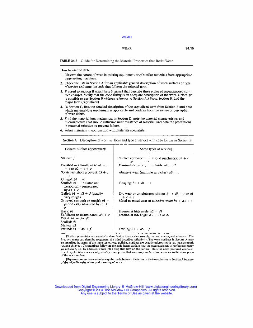
WEAR 34.15
TABLE 34.3 Guide for Determining the Material Properties that Resist Wear
WEAR
Downloaded from Digital Engineering Library @ McGraw-Hill (www.digitalengineeringlibrary.com)Copyright © 2004 The McGraw-Hill Companies. All rights reserved.
Any use is subject to the Terms of Use as given at the website.
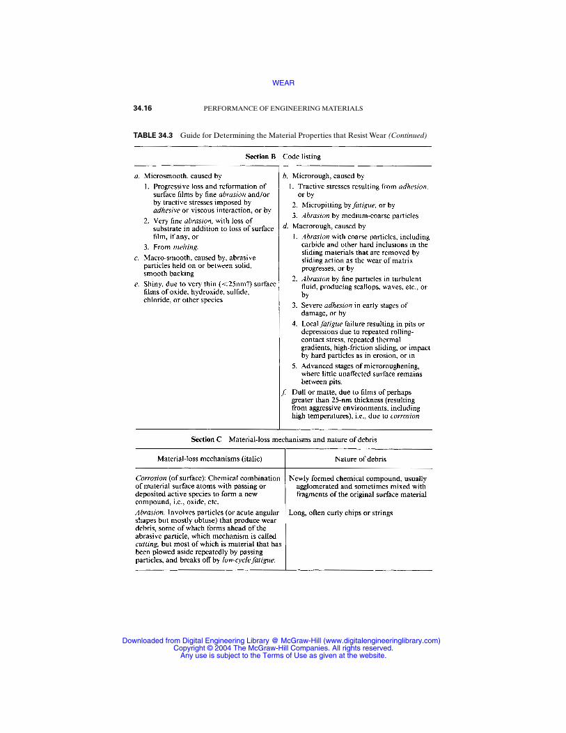
34.16 PERFORMANCE OF ENGINEERING MATERIALS
TABLE 34.3 Guide for Determining the Material Properties that Resist Wear (Continued)
WEAR
Downloaded from Digital Engineering Library @ McGraw-Hill (www.digitalengineeringlibrary.com)Copyright © 2004 The McGraw-Hill Companies. All rights reserved.
Any use is subject to the Terms of Use as given at the website.
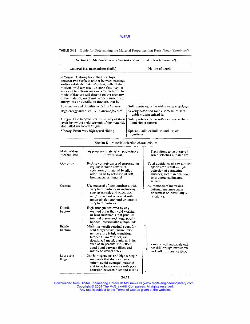
TABLE 34.3 Guide for Determining the Material Properties that Resist Wear (Continued)
34.17
WEAR
Downloaded from Digital Engineering Library @ McGraw-Hill (www.digitalengineeringlibrary.com)Copyright © 2004 The McGraw-Hill Companies. All rights reserved.
Any use is subject to the Terms of Use as given at the website.

REFERENCES
34.1 H. C. Meng and K. C. Ludema, “Wear Models and Predictive Equations: Their Form and Content,” Wear, vol. 181–183, pp. 443–457, 1995.
34.2 K. C. Ludema, “Selecting Materials for Wear Resistance,” Conference on Wear of Materials, San Francisco, 1981, ASME, New York.
BIBLIOGRAPHY
The previous sections are composite views of many authors, so that a reference listwould be very long. Interested readers could consult the many journals containingpapers on wear, but that literature is potentially very confusing. The most usefuljournals are
Wear, Elsevier, Lausanne, starting in 1957.Tribology International, Butterworth Scientific, Ltd., London, starting in 1968.Tribology Transactions of the Society of Tribologists and Lubrication Engineers (formerly
Transactions of the American Society of Lubrication Engineers).Journal of Tribology, also identified as Transactions F, American Society of Mechanical Engi-
neers.
34.18 PERFORMANCE OF ENGINEERING MATERIALS
TABLE 34.3 Guide for Determining the Material Properties that Resist Wear (Continued)
WEAR
Downloaded from Digital Engineering Library @ McGraw-Hill (www.digitalengineeringlibrary.com)Copyright © 2004 The McGraw-Hill Companies. All rights reserved.
Any use is subject to the Terms of Use as given at the website.
CHAPTER 35CORROSION
Milton G. Wille, Ph.D., P.E.Professor of Mechanical Engineering
Brigham Young UniversityProvo, Utah
35.1 INTRODUCTION / 35.1
35.2 CORROSION RATES / 35.2
35.3 METAL ATTACK MECHANISMS / 35.2
35.4 CORROSION DATA FOR MATERIALS SELECTION / 35.28
REFERENCES / 35.28
35.1 INTRODUCTION
Corrosion removal deals with the taking away of mass from the surface of materialsby their environment and other forms of environmental attack that weaken orotherwise degrade material properties. The complex nature of corrosion suggeststhat the designer who is seriously concerned about corrosion review a good readabletext such as Corrosion Engineering by Fontana and Greene [35.1].
Included in this chapter are many corrosion data for selected environments andmaterials. It is always hazardous to select one material in preference to anotherbased only on published data because of inconsistencies in measuring corrosion,lack of completeness in documenting environments, variations in test methods, andpossible publishing errors.These data do not generally indicate how small variationsin temperature or corrosive concentrations might drastically increase or decreasecorrosion rates. Furthermore, they do not account for the influence of other associ-ated materials or how combinations of attack mechanisms may drastically alter agiven material’s behavior. Stray electric currents should be considered along withthe various attack mechanisms included in this chapter. Brevity has required simpli-fication and the exclusion of some phenomena and data which may be important insome applications.
The data included in this chapter are but a fraction of those available. CorrosionGuide by Rabald [35.2] can be a valuable resource because of its extensive coverageof environments and materials.
Again, all corrosion data included in this chapter or published elsewhereshould be used only as a guide for weeding out unsuitable materials or selectingpotentially acceptable candidates. Verification of suitability should be based onactual experience or laboratory experimentation. The inclusion or exclusion ofdata in this chapter should not be interpreted as an endorsement or rejection ofany material.
35.1
Source: STANDARD HANDBOOK OF MACHINE DESIGN
Downloaded from Digital Engineering Library @ McGraw-Hill (www.digitalengineeringlibrary.com)Copyright © 2004 The McGraw-Hill Companies. All rights reserved.
Any use is subject to the Terms of Use as given at the website.
35.2 CORROSION RATES
The vast majority of metal corrosion data in the United States are expressed interms of surface regression rate mpy (mils, or thousands of an inch, per year). Multi-ply mpy by 0.0254 to obtain millimeters per year (mm/yr). To convert to mass-lossrate, multiply the surface regression rate by surface area and material density, usingconsistent units.
Polymer attack typically involves volume changes, usually increases, caused byliquid absorption; reductions in mechanical properties such as yield strength, tensilestrength, flexure strength, and tensile modulus; discoloration; and/or changes in sur-face texture. Certain plastics are degraded by ultraviolet light, which limits their use-fulness in sunlight unless they are pigmented with an opaque substance such aslamp-black carbon.
35.3 METAL ATTACK MECHANISMS
The attack on metals involves oxidation of neutral metal atoms to form positivelycharged ions which either enter into solution or become part of an oxide layer. Thisprocess generates electrons, which must be consumed by other atoms, reducingthem, or making them more negatively charged. Conservation of electrons requiresthat the rate of metal oxidation (corrosion) equal the rate of reduction (absorptionof electrons by other atoms).
35.3.1 General Attack
In general attack, oxidation and reduction occur on the same metal surface, with afairly uniform distribution. Most of the corrosion data in this chapter are for selectedmaterials subject to uniform attack in a given environment.
Once a suitable material is selected, further control of uniform attack can beachieved by coatings, sacrificial anodes (see Galvanic Corrosion), anodic protection(see Passivation), and inhibitors. Coatings are many times multilayered, involvingboth metallic and polymer layers. Inhibitors are additions to liquid environmentsthat remove corrosives from solution, coat metal surfaces to decrease surface reac-tion rates, or otherwise alter the aggressiveness of the environment.
Chemically protective metallic coatings for steels are usually zinc (galvanized) oraluminum (aluminized). Aluminized steel is best for elevated temperatures up to675°C and for severe industrial atmospheres. Both may be deposited by hot dipping,electrochemistry, or arc spraying. Common barrier-type metallic platings are thoseof chromium and nickel.The Environmental Protection Agency has severely limitedor prohibited the use of lead-bearing and cadmium platings and cyanide platingsolutions.
Polymer coatings (such as paints) shield metal surfaces from electron-receivingelements, such as oxygen, reducing corrosion attack rates. Under mild conditions,even “decorative paints” can be effective. Under more severe conditions, thicker andtougher films are used which resist the effects of moisture, heat, chlorides, and/orother undesirable chemicals. Acrylics, alkyds, silicones, and silicone-modified alkydsare the most commonly used finishes for industrial equipment, including farmequipment. The silicones have higher heat resistance, making them useful forheaters, engines, boilers, dryers, furnaces, etc.
35.2 PERFORMANCE OF ENGINEERING MATERIALS
CORROSION
Downloaded from Digital Engineering Library @ McGraw-Hill (www.digitalengineeringlibrary.com)Copyright © 2004 The McGraw-Hill Companies. All rights reserved.
Any use is subject to the Terms of Use as given at the website.
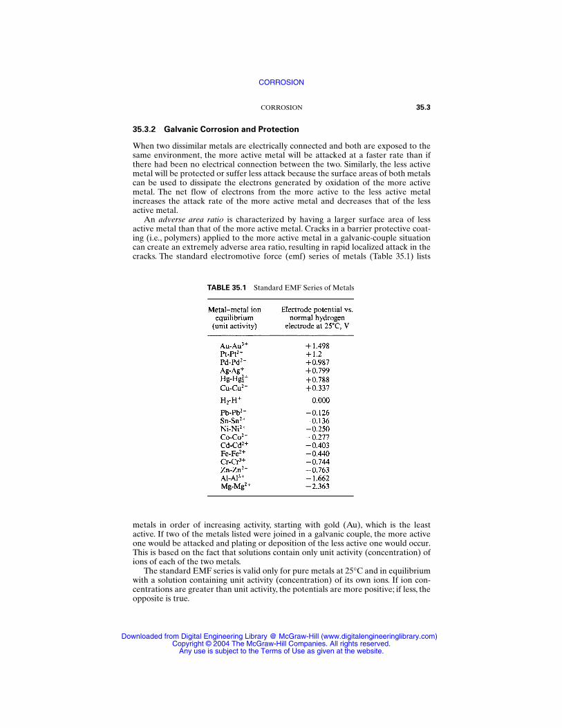
35.3.2 Galvanic Corrosion and Protection
When two dissimilar metals are electrically connected and both are exposed to thesame environment, the more active metal will be attacked at a faster rate than ifthere had been no electrical connection between the two. Similarly, the less activemetal will be protected or suffer less attack because the surface areas of both metalscan be used to dissipate the electrons generated by oxidation of the more activemetal. The net flow of electrons from the more active to the less active metalincreases the attack rate of the more active metal and decreases that of the lessactive metal.
An adverse area ratio is characterized by having a larger surface area of lessactive metal than that of the more active metal. Cracks in a barrier protective coat-ing (i.e., polymers) applied to the more active metal in a galvanic-couple situationcan create an extremely adverse area ratio, resulting in rapid localized attack in thecracks. The standard electromotive force (emf) series of metals (Table 35.1) lists
CORROSION 35.3
TABLE 35.1 Standard EMF Series of Metals
metals in order of increasing activity, starting with gold (Au), which is the leastactive. If two of the metals listed were joined in a galvanic couple, the more activeone would be attacked and plating or deposition of the less active one would occur.This is based on the fact that solutions contain only unit activity (concentration) ofions of each of the two metals.
The standard EMF series is valid only for pure metals at 25°C and in equilibriumwith a solution containing unit activity (concentration) of its own ions. If ion con-centrations are greater than unit activity, the potentials are more positive; if less, theopposite is true.
CORROSION
Downloaded from Digital Engineering Library @ McGraw-Hill (www.digitalengineeringlibrary.com)Copyright © 2004 The McGraw-Hill Companies. All rights reserved.
Any use is subject to the Terms of Use as given at the website.

The galvanic series (Table 35.2) shows a similar relationship, except that impuremetals such as alloys are also included and the medium is seawater. Other media,other concentrations, and other temperatures can further alter the order of the list.Therefore, care should be exercised in applying these data to a given galvanic corro-sion situation except as a general, loose guide.
35.3.3 Passivation
Certain common engineering materials, such as iron, nickel, chromium, titanium,and silicon as well as their alloys (i.e., stainless steels), exhibit a characteristic ofbeing able to behave both as a more active and as a less active (passive) material.
35.4 PERFORMANCE OF ENGINEERING MATERIALS
TABLE 35.2 Galvanic Series of Some Commercial Metals and Alloysin Seawater
CORROSION
Downloaded from Digital Engineering Library @ McGraw-Hill (www.digitalengineeringlibrary.com)Copyright © 2004 The McGraw-Hill Companies. All rights reserved.
Any use is subject to the Terms of Use as given at the website.
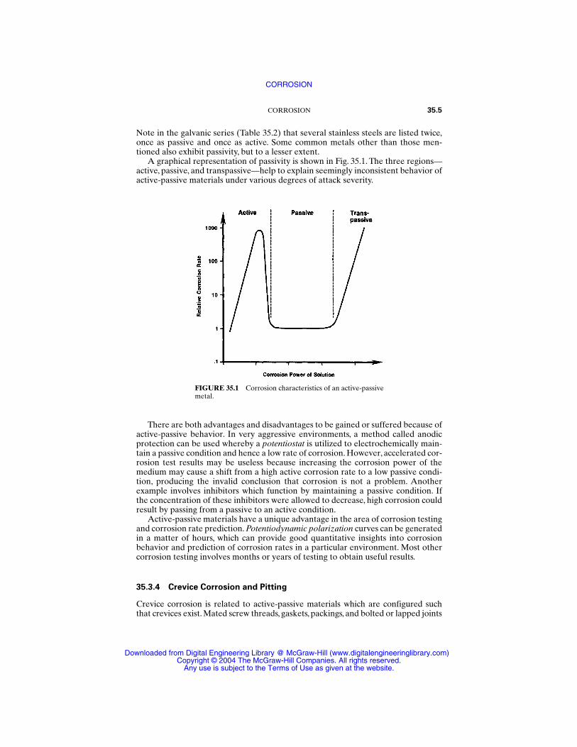
Note in the galvanic series (Table 35.2) that several stainless steels are listed twice,once as passive and once as active. Some common metals other than those men-tioned also exhibit passivity, but to a lesser extent.
A graphical representation of passivity is shown in Fig. 35.1. The three regions—active, passive, and transpassive—help to explain seemingly inconsistent behavior ofactive-passive materials under various degrees of attack severity.
CORROSION 35.5
FIGURE 35.1 Corrosion characteristics of an active-passivemetal.
There are both advantages and disadvantages to be gained or suffered because ofactive-passive behavior. In very aggressive environments, a method called anodicprotection can be used whereby a potentiostat is utilized to electrochemically main-tain a passive condition and hence a low rate of corrosion. However, accelerated cor-rosion test results may be useless because increasing the corrosion power of themedium may cause a shift from a high active corrosion rate to a low passive condi-tion, producing the invalid conclusion that corrosion is not a problem. Anotherexample involves inhibitors which function by maintaining a passive condition. Ifthe concentration of these inhibitors were allowed to decrease, high corrosion couldresult by passing from a passive to an active condition.
Active-passive materials have a unique advantage in the area of corrosion testingand corrosion rate prediction. Potentiodynamic polarization curves can be generatedin a matter of hours, which can provide good quantitative insights into corrosionbehavior and prediction of corrosion rates in a particular environment. Most othercorrosion testing involves months or years of testing to obtain useful results.
35.3.4 Crevice Corrosion and Pitting
Crevice corrosion is related to active-passive materials which are configured suchthat crevices exist. Mated screw threads, gaskets, packings, and bolted or lapped joints
CORROSION
Downloaded from Digital Engineering Library @ McGraw-Hill (www.digitalengineeringlibrary.com)Copyright © 2004 The McGraw-Hill Companies. All rights reserved.
Any use is subject to the Terms of Use as given at the website.

are common examples of crevices. Inside the crevice, oxygen or other corrosivesrequired for passivation have restricted entrance, resulting in reduced concentrationas they are consumed by corrosion in the crevice. When the concentration of thesecorrosives is low enough to fail to maintain passivity, the metal in the crevice becomesactive. The large electrically connected, passivated surface outside the crevice com-pletes a galvanic couple with a large adverse-area ratio, providing high attack rateswithin the crevice.Welding or forming can be used to avoid crevices. However, inter-granular corrosion may occur in welded stainless steels (see Sec. 35.3.9).
Pitting is a very localized attack that results in holes, or voids, on a metal surface.Although not restricted to active-passive metals, pitting is commonly related tothese. With active-passive metals, pieces of dirt, scale, or other solid particles mayrest on the bottom of a pipe or tank where velocities are not sufficient to movethem. These particles form crevices, resulting in a localized attack similar to crevicecorrosion.
35.3.5 Sacrificial Anodes
Magnesium rods are placed in steel glass-lined hot-water tanks, and zinc is used tocoat sheet steel (galvanized steel) to provide protection to the steel against cor-rosion. As the more active magnesium rod is attacked, the electrons generated are conveyed to the electrically connected steel tank, which needs protection onlyfor regions where cracks or flaws exist in the glass lining. Similarly, for galvanizedsteel, protection is required only for regions of scratches or where steel edges areexposed.
35.3.6 Stress Corrosion Cracking
In stress corrosion cracking (SCC), most of a metal’s surface may show little attack,while fine intergranular or transgranular cracks may penetrate deeply into the sur-face. There may be a single continuous crack or a multibranched crack, or the entiresurface may be covered with a lacy network of cracks. Usually dye penetrants andsectioning are needed to reveal the extent and depth of cracking.
Certain classes of alloys and environments are susceptible to this phenomenon,and usually tensile stresses are involved, with crack penetration rates increasingwith increasing tensile stress. The higher the strength condition of a given alloy, thegreater seems to be the tendency to suffer SCC. Table 35.3 lists some materials andenvironments that have been known to produce SCC.
Frequently, a difference in color or texture is noticeable between a stress corro-sion crack and an adjacent region of overstress when the fracture is completed bymechanical means. Scanning electron micrographs are frequently useful in identify-ing SCC.
35.3.7 Selective Leaching
Selective leaching refers to the chemical removal of one metal from an alloy, result-ing in a weak, porous structure. Brass sink traps suffer this type of attack by zincbeing leached out of the yellow brass, leaving behind a porous structure of reddishcopper. Aluminum and silicon bronzes and other alloys are also subjected to selec-tive leaching.
35.6 PERFORMANCE OF ENGINEERING MATERIALS
CORROSION
Downloaded from Digital Engineering Library @ McGraw-Hill (www.digitalengineeringlibrary.com)Copyright © 2004 The McGraw-Hill Companies. All rights reserved.
Any use is subject to the Terms of Use as given at the website.
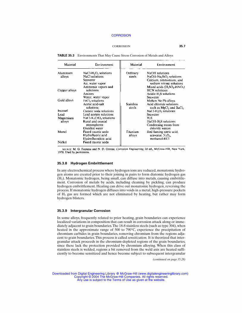
35.3.8 Hydrogen Embrittlement
In any electrochemical process where hydrogen ions are reduced, monatomic hydro-gen atoms are created prior to their joining in pairs to form diatomic hydrogen gas(H2). Monatomic hydrogen, being small, can diffuse into metals, causing embrittle-ment. Corrosion of metals by acids, including cleaning by pickling, can producehydrogen embrittlement. Heating can drive out monatomic hydrogen, reversing theprocess. If monatomic hydrogen diffuses into voids in a metal, high-pressure pocketsof H2 gas are formed which are not eliminated by heating, but rather may formhydrogen blisters.
35.3.9 Intergranular Corrosion
In some alloys, frequently related to prior heating, grain boundaries can experiencelocalized variations in composition that can result in corrosion attack along or imme-diately adjacent to grain boundaries.The 18-8 stainless steels (such as type 304), whenheated in the approximate range of 500 to 790°C, experience the precipitation ofchromium carbides in grain boundaries, removing chromium from the regions adja-cent to grain boundaries.This process is called sensitization. It is theorized that inter-granular attack proceeds in the chromium-depleted regions of the grain boundaries,since these lack the protection provided by chromium alloying. When this class ofstainless steels is welded, regions a bit removed from the weld axis are heated suffi-ciently to become sensitized and hence become subject to subsequent intergranular
(continued on page 35.28)
CORROSION 35.7
TABLE 35.3 Environments That May Cause Stress Corrosion of Metals and Alloys
CORROSION
Downloaded from Digital Engineering Library @ McGraw-Hill (www.digitalengineeringlibrary.com)Copyright © 2004 The McGraw-Hill Companies. All rights reserved.
Any use is subject to the Terms of Use as given at the website.
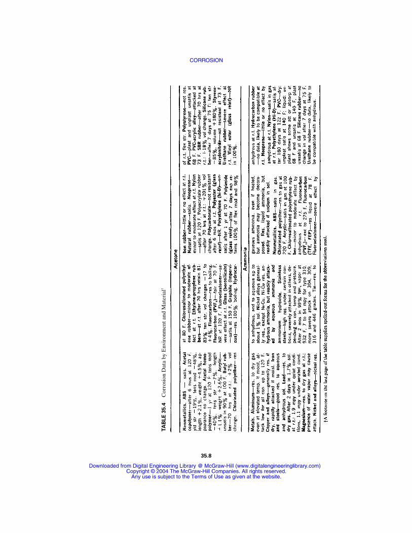
TA
BLE
35.4
Cor
rosi
on D
ata
by E
nvir
onm
ent a
nd M
ater
ial†
35.8
CORROSION
Downloaded from Digital Engineering Library @ McGraw-Hill (www.digitalengineeringlibrary.com)Copyright © 2004 The McGraw-Hill Companies. All rights reserved.
Any use is subject to the Terms of Use as given at the website.
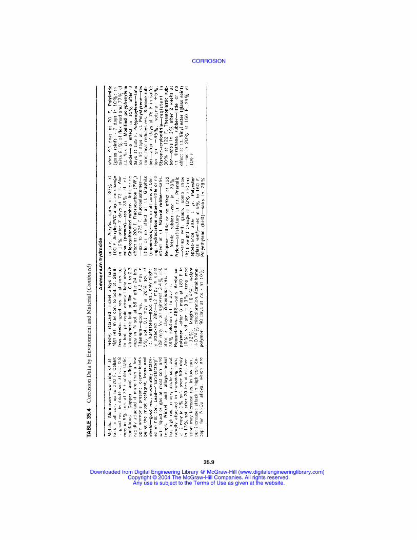
35.9
TA
BLE
35.4
Cor
rosi
on D
ata
by E
nvir
onm
ent a
nd M
ater
ial (
Con
tinue
d)
CORROSION
Downloaded from Digital Engineering Library @ McGraw-Hill (www.digitalengineeringlibrary.com)Copyright © 2004 The McGraw-Hill Companies. All rights reserved.
Any use is subject to the Terms of Use as given at the website.
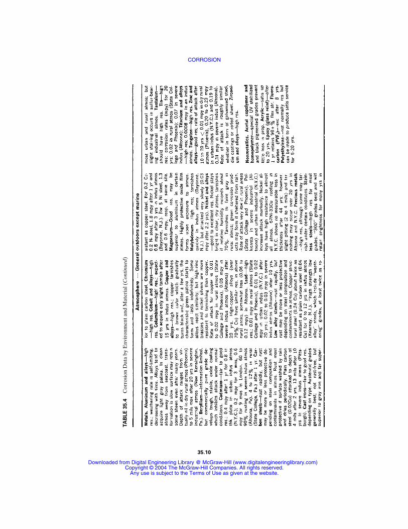
TA
BLE
35.4
Cor
rosi
on D
ata
by E
nvir
onm
ent a
nd M
ater
ial (
Con
tinue
d)
35.10
CORROSION
Downloaded from Digital Engineering Library @ McGraw-Hill (www.digitalengineeringlibrary.com)Copyright © 2004 The McGraw-Hill Companies. All rights reserved.
Any use is subject to the Terms of Use as given at the website.
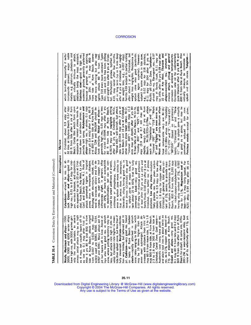
35.11
TA
BLE
35.4
Cor
rosi
on D
ata
by E
nvir
onm
ent a
nd M
ater
ial (
Con
tinue
d)
CORROSION
Downloaded from Digital Engineering Library @ McGraw-Hill (www.digitalengineeringlibrary.com)Copyright © 2004 The McGraw-Hill Companies. All rights reserved.
Any use is subject to the Terms of Use as given at the website.
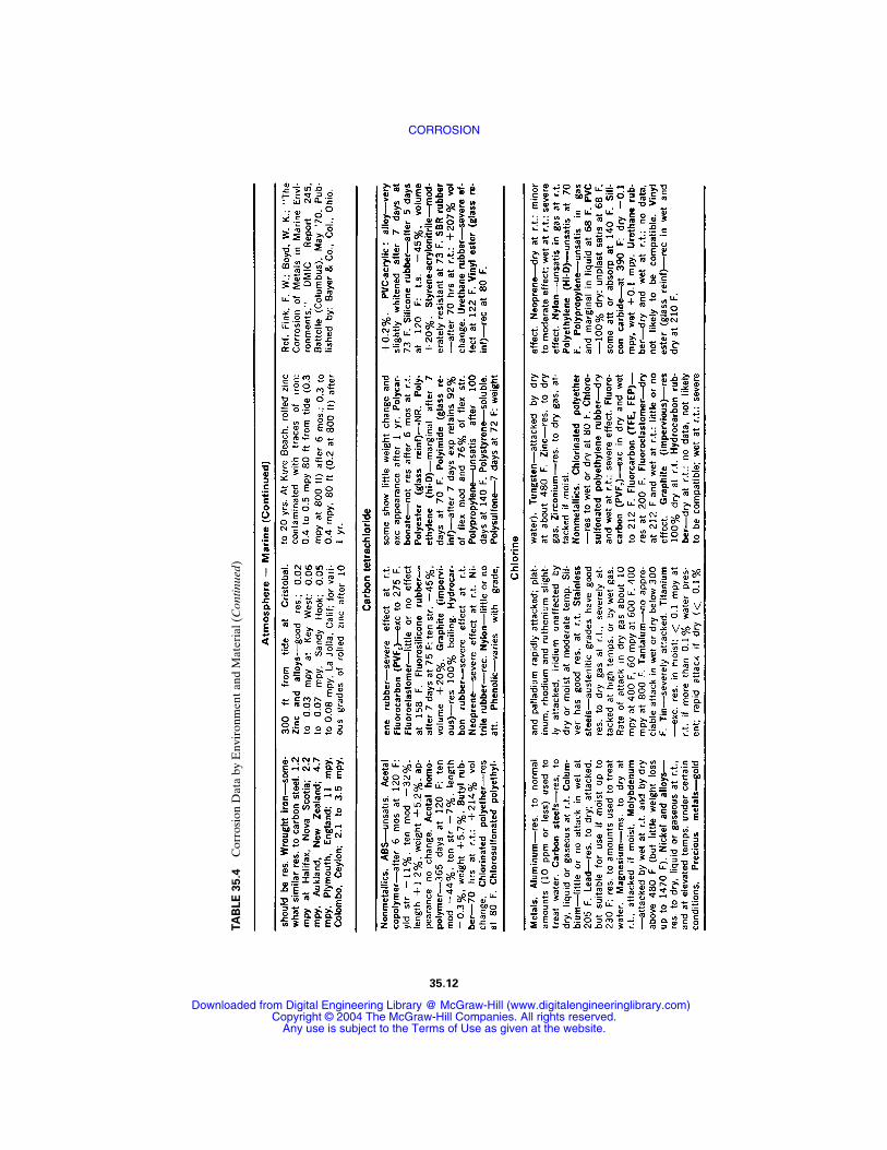
TA
BLE
35.4
Cor
rosi
on D
ata
by E
nvir
onm
ent a
nd M
ater
ial (
Con
tinue
d)
35.12
CORROSION
Downloaded from Digital Engineering Library @ McGraw-Hill (www.digitalengineeringlibrary.com)Copyright © 2004 The McGraw-Hill Companies. All rights reserved.
Any use is subject to the Terms of Use as given at the website.
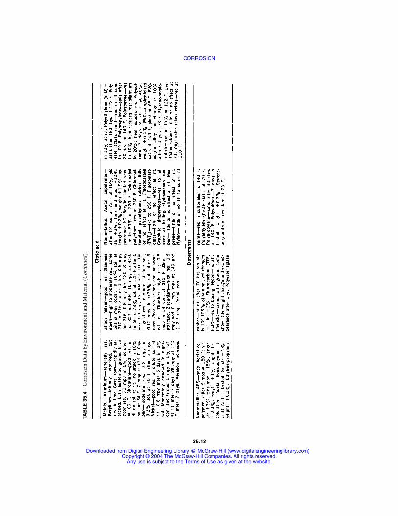
35.13
TA
BLE
35.4
Cor
rosi
on D
ata
by E
nvir
onm
ent a
nd M
ater
ial (
Con
tinue
d)
CORROSION
Downloaded from Digital Engineering Library @ McGraw-Hill (www.digitalengineeringlibrary.com)Copyright © 2004 The McGraw-Hill Companies. All rights reserved.
Any use is subject to the Terms of Use as given at the website.
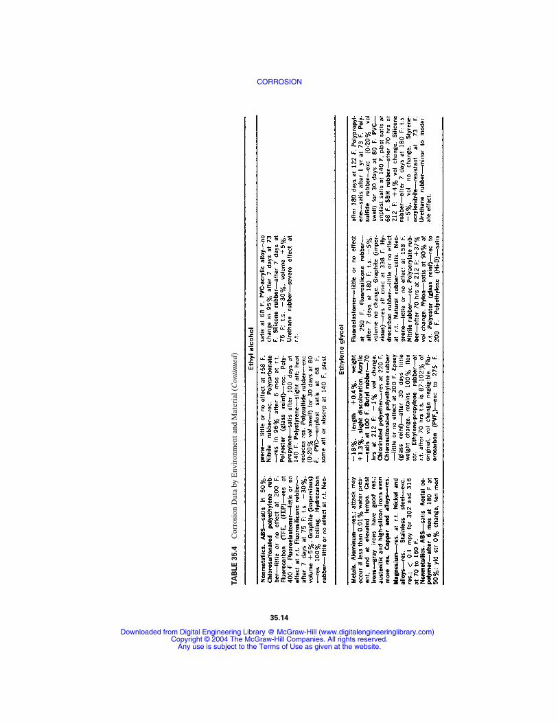
TA
BLE
35.4
Cor
rosi
on D
ata
by E
nvir
onm
ent a
nd M
ater
ial (
Con
tinue
d)
35.14
CORROSION
Downloaded from Digital Engineering Library @ McGraw-Hill (www.digitalengineeringlibrary.com)Copyright © 2004 The McGraw-Hill Companies. All rights reserved.
Any use is subject to the Terms of Use as given at the website.
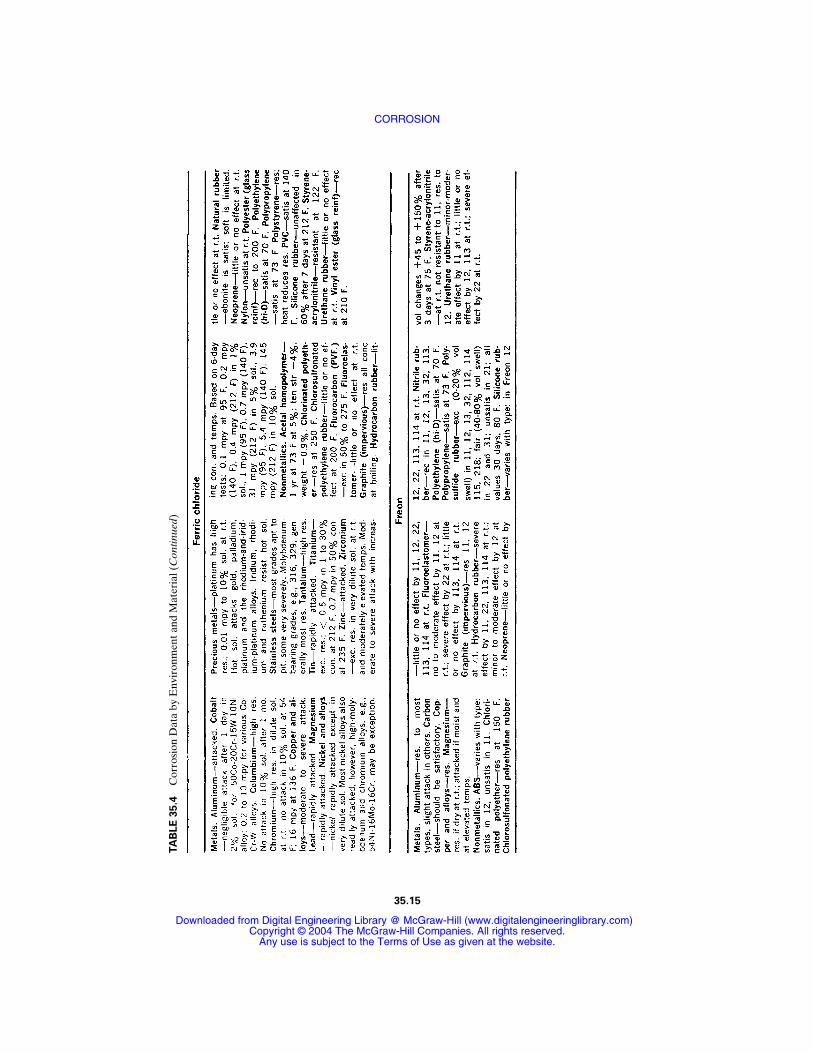
35.15
TA
BLE
35.4
Cor
rosi
on D
ata
by E
nvir
onm
ent a
nd M
ater
ial (
Con
tinue
d)
CORROSION
Downloaded from Digital Engineering Library @ McGraw-Hill (www.digitalengineeringlibrary.com)Copyright © 2004 The McGraw-Hill Companies. All rights reserved.
Any use is subject to the Terms of Use as given at the website.
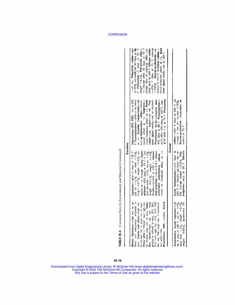
TA
BLE
35.4
Cor
rosi
on D
ata
by E
nvir
onm
ent a
nd M
ater
ial (
Con
tinue
d)
35.16
CORROSION
Downloaded from Digital Engineering Library @ McGraw-Hill (www.digitalengineeringlibrary.com)Copyright © 2004 The McGraw-Hill Companies. All rights reserved.
Any use is subject to the Terms of Use as given at the website.
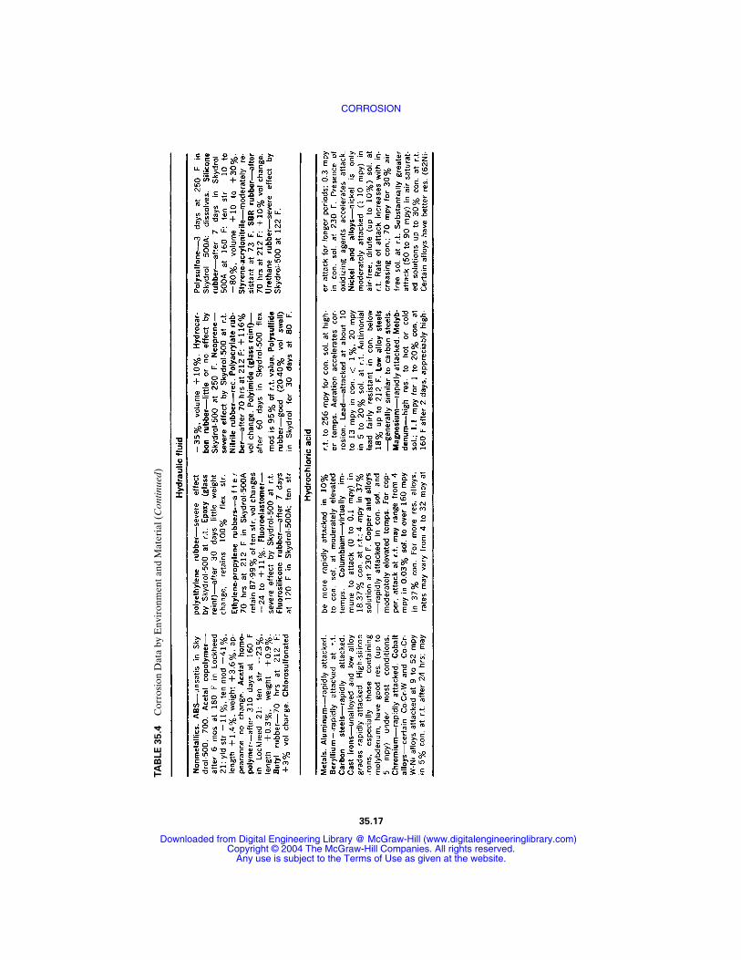
35.17
TA
BLE
35.4
Cor
rosi
on D
ata
by E
nvir
onm
ent a
nd M
ater
ial (
Con
tinue
d)
CORROSION
Downloaded from Digital Engineering Library @ McGraw-Hill (www.digitalengineeringlibrary.com)Copyright © 2004 The McGraw-Hill Companies. All rights reserved.
Any use is subject to the Terms of Use as given at the website.
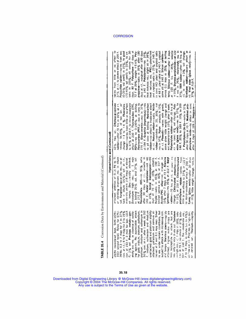
TA
BLE
35.4
Cor
rosi
on D
ata
by E
nvir
onm
ent a
nd M
ater
ial (
Con
tinue
d)
35.18
CORROSION
Downloaded from Digital Engineering Library @ McGraw-Hill (www.digitalengineeringlibrary.com)Copyright © 2004 The McGraw-Hill Companies. All rights reserved.
Any use is subject to the Terms of Use as given at the website.
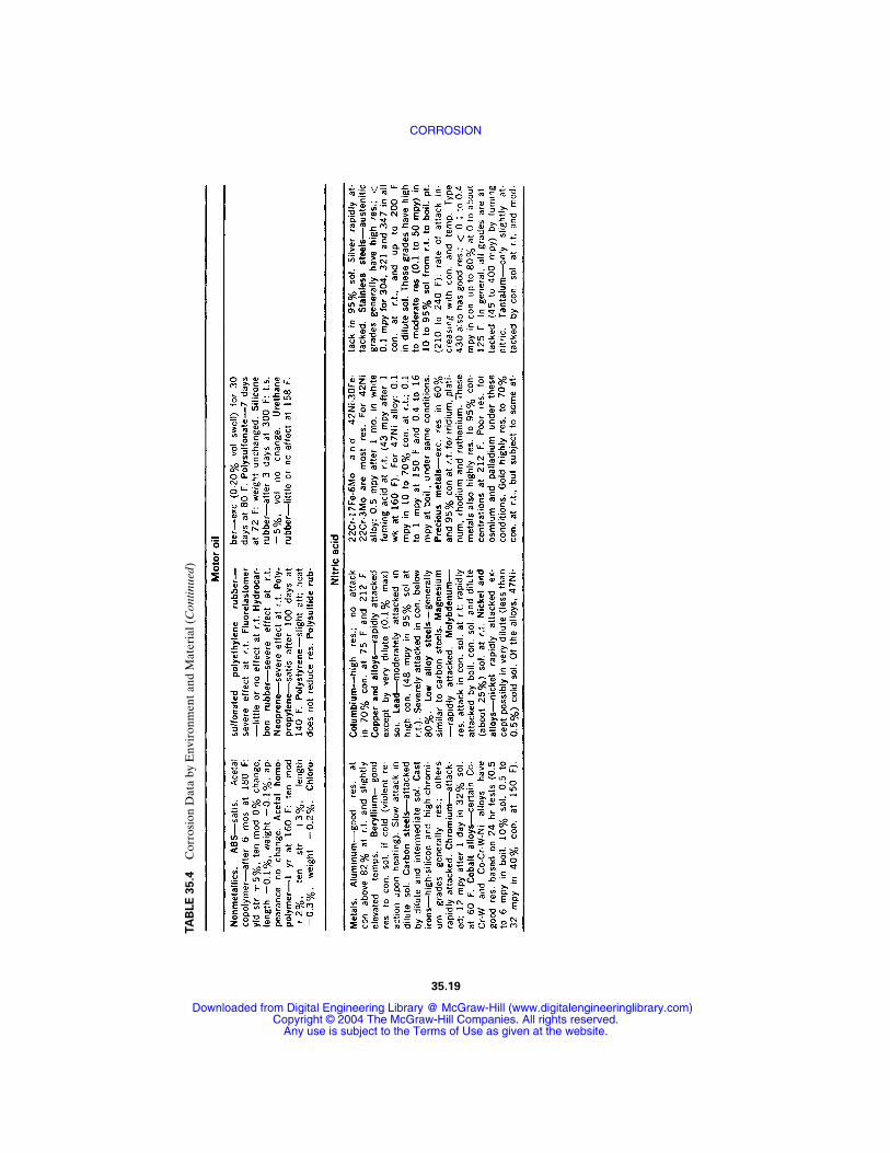
35.19
TA
BLE
35.4
Cor
rosi
on D
ata
by E
nvir
onm
ent a
nd M
ater
ial (
Con
tinue
d)
CORROSION
Downloaded from Digital Engineering Library @ McGraw-Hill (www.digitalengineeringlibrary.com)Copyright © 2004 The McGraw-Hill Companies. All rights reserved.
Any use is subject to the Terms of Use as given at the website.
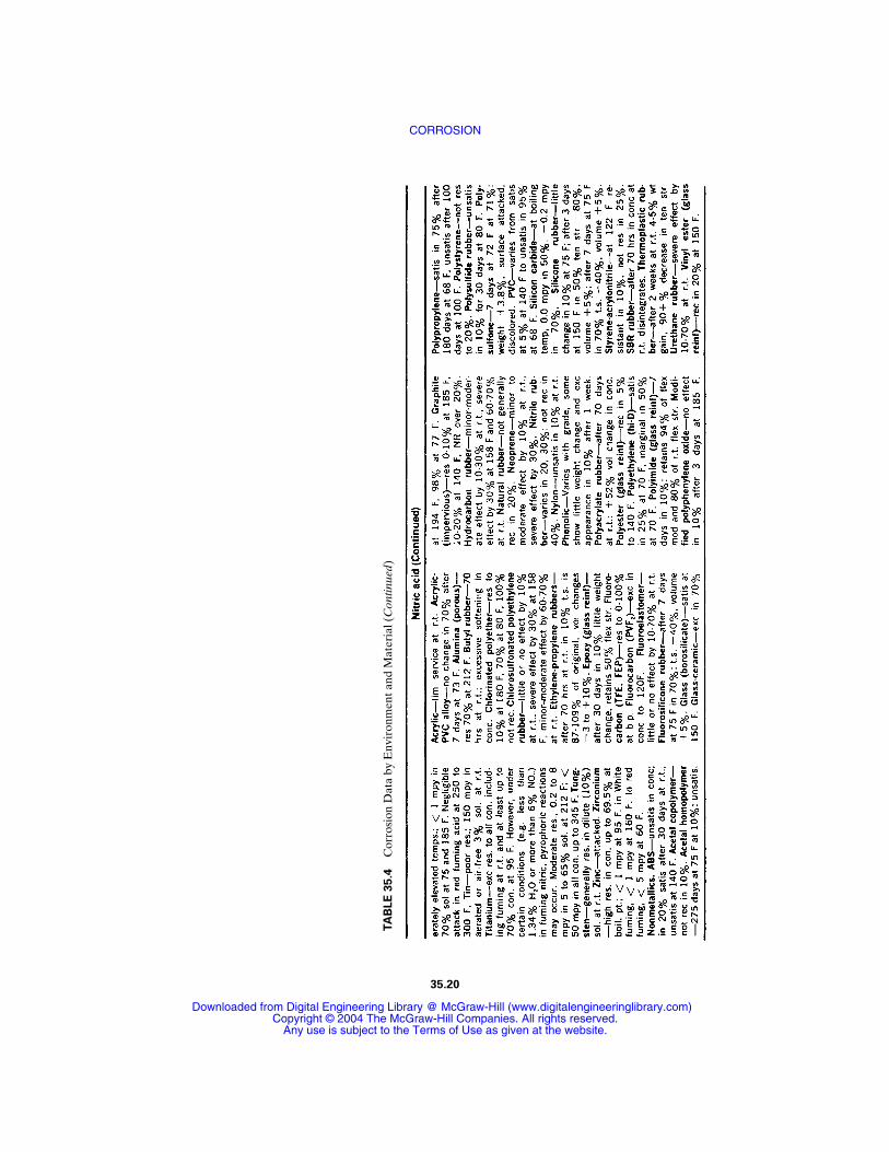
TA
BLE
35.4
Cor
rosi
on D
ata
by E
nvir
onm
ent a
nd M
ater
ial (
Con
tinue
d)
35.20
CORROSION
Downloaded from Digital Engineering Library @ McGraw-Hill (www.digitalengineeringlibrary.com)Copyright © 2004 The McGraw-Hill Companies. All rights reserved.
Any use is subject to the Terms of Use as given at the website.
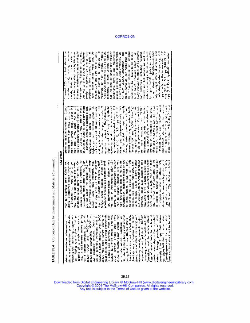
35.21
TA
BLE
35.4
Cor
rosi
on D
ata
by E
nvir
onm
ent a
nd M
ater
ial (
Con
tinue
d)
CORROSION
Downloaded from Digital Engineering Library @ McGraw-Hill (www.digitalengineeringlibrary.com)Copyright © 2004 The McGraw-Hill Companies. All rights reserved.
Any use is subject to the Terms of Use as given at the website.
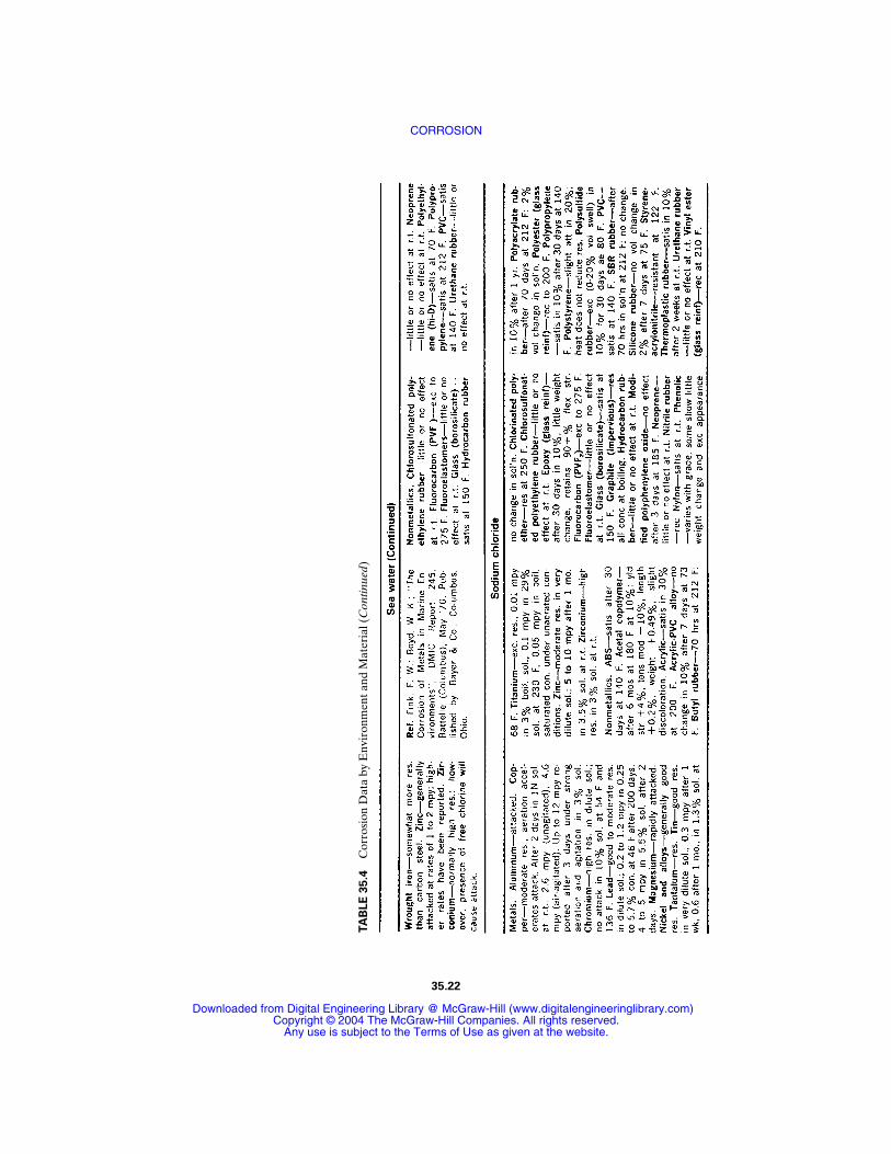
TA
BLE
35.4
Cor
rosi
on D
ata
by E
nvir
onm
ent a
nd M
ater
ial (
Con
tinue
d)
35.22
CORROSION
Downloaded from Digital Engineering Library @ McGraw-Hill (www.digitalengineeringlibrary.com)Copyright © 2004 The McGraw-Hill Companies. All rights reserved.
Any use is subject to the Terms of Use as given at the website.
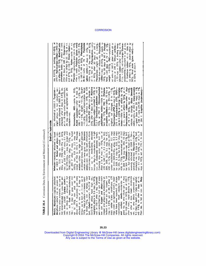
35.23
TA
BLE
35.4
Cor
rosi
on D
ata
by E
nvir
onm
ent a
nd M
ater
ial (
Con
tinue
d)
CORROSION
Downloaded from Digital Engineering Library @ McGraw-Hill (www.digitalengineeringlibrary.com)Copyright © 2004 The McGraw-Hill Companies. All rights reserved.
Any use is subject to the Terms of Use as given at the website.
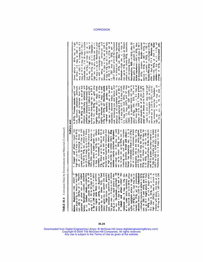
TA
BLE
35.4
Cor
rosi
on D
ata
by E
nvir
onm
ent a
nd M
ater
ial (
Con
tinue
d)
35.24
CORROSION
Downloaded from Digital Engineering Library @ McGraw-Hill (www.digitalengineeringlibrary.com)Copyright © 2004 The McGraw-Hill Companies. All rights reserved.
Any use is subject to the Terms of Use as given at the website.
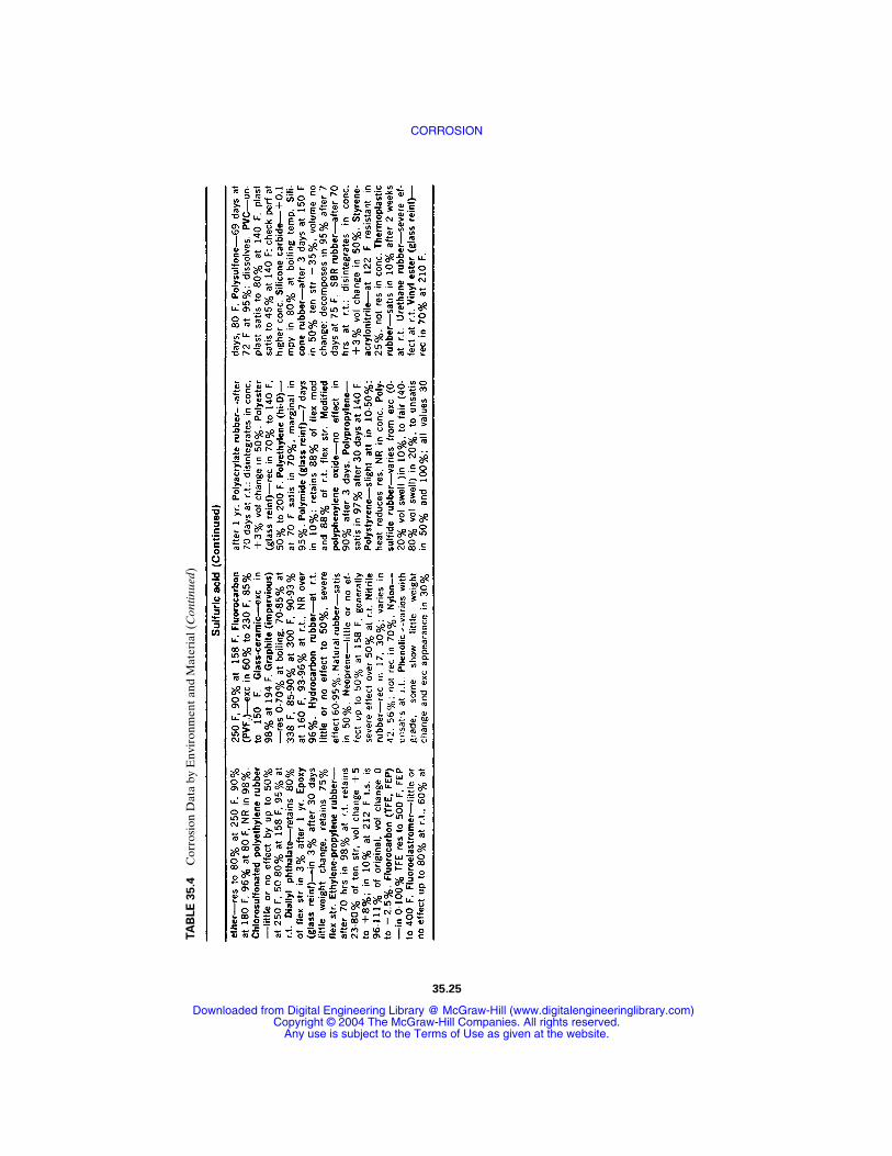
35.25
TA
BLE
35.4
Cor
rosi
on D
ata
by E
nvir
onm
ent a
nd M
ater
ial (
Con
tinue
d)
CORROSION
Downloaded from Digital Engineering Library @ McGraw-Hill (www.digitalengineeringlibrary.com)Copyright © 2004 The McGraw-Hill Companies. All rights reserved.
Any use is subject to the Terms of Use as given at the website.
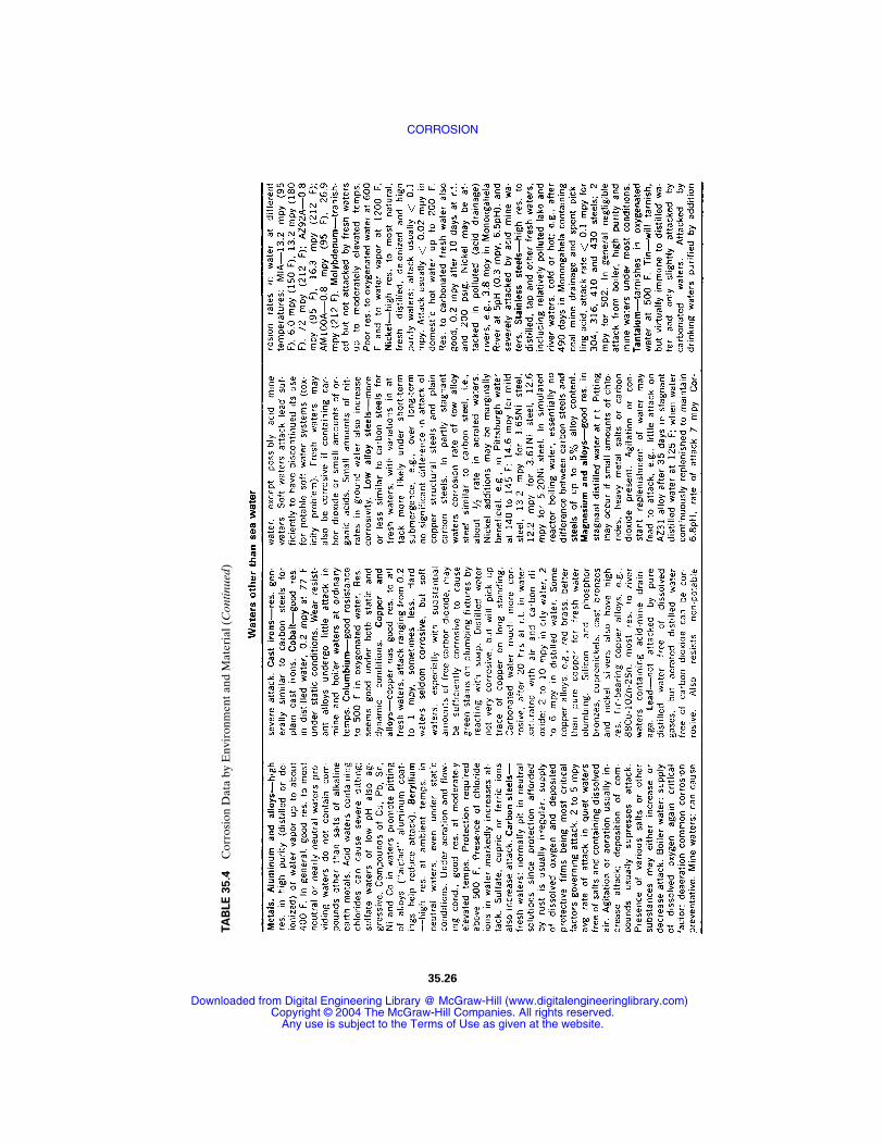
TA
BLE
35.4
Cor
rosi
on D
ata
by E
nvir
onm
ent a
nd M
ater
ial (
Con
tinue
d)
35.26
CORROSION
Downloaded from Digital Engineering Library @ McGraw-Hill (www.digitalengineeringlibrary.com)Copyright © 2004 The McGraw-Hill Companies. All rights reserved.
Any use is subject to the Terms of Use as given at the website.
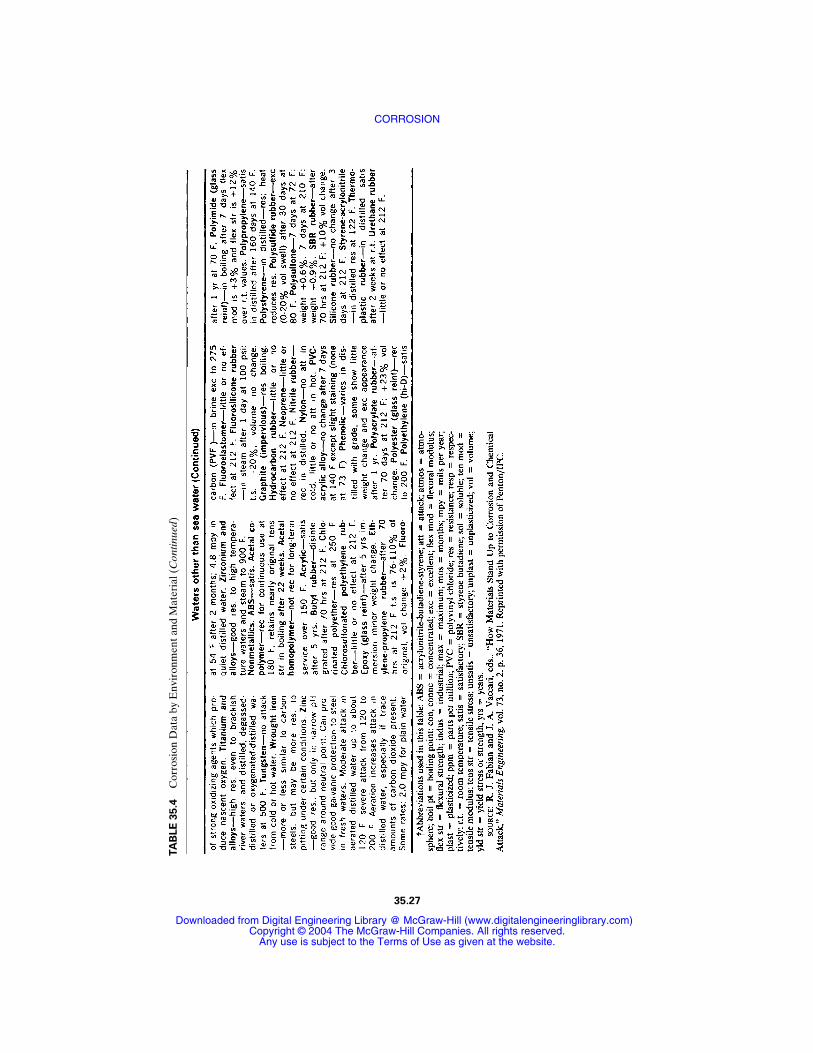
35.27
TA
BLE
35.4
Cor
rosi
on D
ata
by E
nvir
onm
ent a
nd M
ater
ial (
Con
tinue
d)
CORROSION
Downloaded from Digital Engineering Library @ McGraw-Hill (www.digitalengineeringlibrary.com)Copyright © 2004 The McGraw-Hill Companies. All rights reserved.
Any use is subject to the Terms of Use as given at the website.

corrosion (weld decay). Heating to higher temperatures, 1060 to 1120°C, followed bywater quenching will redissolve the precipitated carbides and keep them in solution.Appropriate alloying changes can reduce carbide precipitation.
35.3.10 Mechanical Contributions
Fluid flow or mechanical rubbing can cause removal of or damage to a protectiveoxide, increasing the proximity of the bare metal and the attacking medium.This canresult in increased attack rates because a stable oxide layer is frequently a corrosionrate limiter. An example is erosion corrosion caused by high flow rates of domestichot water in copper pipes, especially around fittings, which can generate turbulence.Another example involves the press fit of gears, wheels, pulleys, etc., onto shafts thatexperience elastic torsion, or bending. Small relative motions occur at the contactingsurfaces which mechanically break up protective oxide layers.This type of corrosionis known as fretting corrosion.
35.4 CORROSION DATA FOR MATERIALS SELECTION†
Subject to the limitations mentioned at the beginning of this chapter, the corrosiondata in Table 35.4 can be used as a guide in selecting materials for the environmentslisted. The organization is first by environments and then by materials, metals fol-lowed by nonmetals. The abbreviation NR means not recommended.
REFERENCES
35.1 M. G. Fontana and N. D. Greene, Corrosion Engineering, 2d ed., McGraw-Hill, NewYork, 1978.
35.2 E. Rabald, Corrosion Guide, 2d ed., rev., Elsevier Scientific Publishing, Amsterdam,1968.
35.3 R. J. Fabian and J. A. Vaccari (eds.), “How Materials Stand Up to Corrosion and Chemi-cal Attack,” Materials Engineering, vol. 73, no. 2, February 1971, p. 36.
35.28 PERFORMANCE OF ENGINEERING MATERIALS
CORROSION
Downloaded from Digital Engineering Library @ McGraw-Hill (www.digitalengineeringlibrary.com)Copyright © 2004 The McGraw-Hill Companies. All rights reserved.
Any use is subject to the Terms of Use as given at the website.

P • A • R • T • 9
CLASSICAL STRESSAND DEFORMATION
ANALYSIS
Source: STANDARD HANDBOOK OF MACHINE DESIGN
Downloaded from Digital Engineering Library @ McGraw-Hill (www.digitalengineeringlibrary.com)Copyright © 2004 The McGraw-Hill Companies. All rights reserved.
Any use is subject to the Terms of Use as given at the website.

CLASSICAL STRESS AND DEFORMATION ANALYSIS
Downloaded from Digital Engineering Library @ McGraw-Hill (www.digitalengineeringlibrary.com)Copyright © 2004 The McGraw-Hill Companies. All rights reserved.
Any use is subject to the Terms of Use as given at the website.
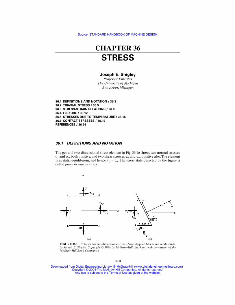
CHAPTER 36STRESS
Joseph E. ShigleyProfessor Emeritus
The University of MichiganAnn Arbor, Michigan
36.1 DEFINITIONS AND NOTATION / 36.3
36.2 TRIAXIAL STRESS / 36.5
36.3 STRESS-STRAIN RELATIONS / 36.6
36.4 FLEXURE / 36.12
36.5 STRESSES DUE TO TEMPERATURE / 36.16
36.6 CONTACT STRESSES / 36.19
REFERENCES / 36.24
36.1 DEFINITIONS AND NOTATION
The general two-dimensional stress element in Fig. 36.1a shows two normal stressesσx and σy, both positive, and two shear stresses τxy and τyx, positive also. The elementis in static equilibrium, and hence τxy = τyx. The stress state depicted by the figure iscalled plane or biaxial stress.
36.3
FIGURE 36.1 Notation for two-dimensional stress. (From Applied Mechanics of Materials,by Joseph E. Shigley. Copyright © 1976 by McGraw-Hill, Inc. Used with permission of theMcGraw-Hill Book Company.)
(a) (b)
Source: STANDARD HANDBOOK OF MACHINE DESIGN
Downloaded from Digital Engineering Library @ McGraw-Hill (www.digitalengineeringlibrary.com)Copyright © 2004 The McGraw-Hill Companies. All rights reserved.
Any use is subject to the Terms of Use as given at the website.
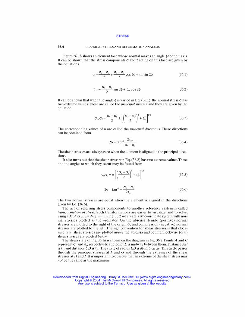
Figure 36.1b shows an element face whose normal makes an angle φ to the x axis.It can be shown that the stress components σ and τ acting on this face are given bythe equations
σ = σx +
2σy
+ σx −
2σy
cos 2φ + τxy sin 2φ (36.1)
τ = − σx −
2σy
sin 2φ + τxy cos 2φ (36.2)
It can be shown that when the angle φ is varied in Eq. (36.1), the normal stress σ hastwo extreme values. These are called the principal stresses, and they are given by theequation
σ1, σ2 = σx +
2σy
± σx −2
σy
2
+ τxy2
1/2
(36.3)
The corresponding values of φ are called the principal directions. These directionscan be obtained from
2φ = tan−1 (36.4)
The shear stresses are always zero when the element is aligned in the principal direc-tions.
It also turns out that the shear stress τ in Eq. (36.2) has two extreme values.Theseand the angles at which they occur may be found from
τ1, τ2 = ± σx −2
σy
2
+ τxy2
1/2
(36.5)
2φ = tan−1 − σx
2−τxy
σy (36.6)
The two normal stresses are equal when the element is aligned in the directionsgiven by Eq. (36.6).
The act of referring stress components to another reference system is calledtransformation of stress. Such transformations are easier to visualize, and to solve,using a Mohr’s circle diagram. In Fig. 36.2 we create a στ coordinate system with nor-mal stresses plotted as the ordinates. On the abscissa, tensile (positive) normalstresses are plotted to the right of the origin O, and compression (negative) normalstresses are plotted to the left. The sign convention for shear stresses is that clock-wise (cw) shear stresses are plotted above the abscissa and counterclockwise (ccw)shear stresses are plotted below.
The stress state of Fig. 36.1a is shown on the diagram in Fig. 36.2. Points A and Crepresent σx and σy, respectively, and point E is midway between them. Distance ABis τxy and distance CD is τyx. The circle of radius ED is Mohr’s circle. This circle passesthrough the principal stresses at F and G and through the extremes of the shearstresses at H and I. It is important to observe that an extreme of the shear stress maynot be the same as the maximum.
2τxyσx − σy
36.4 CLASSICAL STRESS AND DEFORMATION ANALYSIS
STRESS
Downloaded from Digital Engineering Library @ McGraw-Hill (www.digitalengineeringlibrary.com)Copyright © 2004 The McGraw-Hill Companies. All rights reserved.
Any use is subject to the Terms of Use as given at the website.
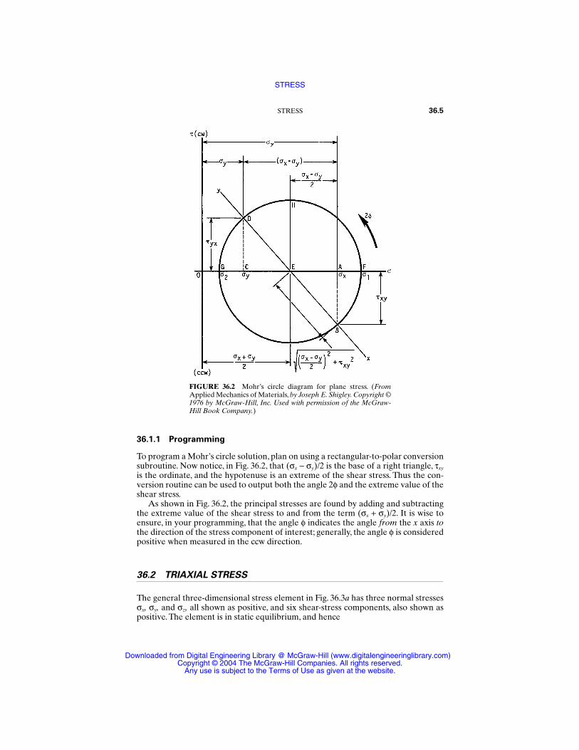
36.1.1 Programming
To program a Mohr’s circle solution, plan on using a rectangular-to-polar conversionsubroutine. Now notice, in Fig. 36.2, that (σx − σy)/2 is the base of a right triangle, τxy
is the ordinate, and the hypotenuse is an extreme of the shear stress. Thus the con-version routine can be used to output both the angle 2φ and the extreme value of theshear stress.
As shown in Fig. 36.2, the principal stresses are found by adding and subtractingthe extreme value of the shear stress to and from the term (σx + σy)/2. It is wise toensure, in your programming, that the angle φ indicates the angle from the x axis tothe direction of the stress component of interest; generally, the angle φ is consideredpositive when measured in the ccw direction.
36.2 TRIAXIAL STRESS
The general three-dimensional stress element in Fig. 36.3a has three normal stressesσx, σy, and σz, all shown as positive, and six shear-stress components, also shown aspositive. The element is in static equilibrium, and hence
STRESS 36.5
FIGURE 36.2 Mohr’s circle diagram for plane stress. (FromApplied Mechanics of Materials, by Joseph E. Shigley. Copyright ©1976 by McGraw-Hill, Inc. Used with permission of the McGraw-Hill Book Company.)
STRESS
Downloaded from Digital Engineering Library @ McGraw-Hill (www.digitalengineeringlibrary.com)Copyright © 2004 The McGraw-Hill Companies. All rights reserved.
Any use is subject to the Terms of Use as given at the website.
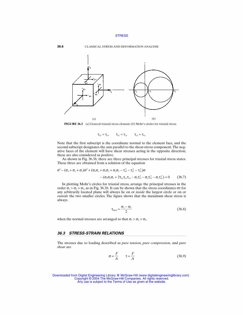
τxy = τyx τyz = τzy τzx = τxz
Note that the first subscript is the coordinate normal to the element face, and thesecond subscript designates the axis parallel to the shear-stress component.The neg-ative faces of the element will have shear stresses acting in the opposite direction;these are also considered as positive.
As shown in Fig. 36.3b, there are three principal stresses for triaxial stress states.These three are obtained from a solution of the equation
σ3 − (σx + σy + σz)σ2 + (σxσy + σxσz + σyσz − τxy2 − τyz
2 − τzx2 )σ
− (σxσyσz + 2τxyτyzτzx − σxτyz2 − σyτzx
2 − σzτxy2 ) = 0 (36.7)
In plotting Mohr’s circles for triaxial stress, arrange the principal stresses in theorder σ1 > σ2 > σ3, as in Fig. 36.3b. It can be shown that the stress coordinates στ forany arbitrarily located plane will always lie on or inside the largest circle or on oroutside the two smaller circles. The figure shows that the maximum shear stress isalways
τmax = σ1 −
2σ3
(36.8)
when the normal stresses are arranged so that σ1 > σ2 > σ3.
36.3 STRESS-STRAIN RELATIONS
The stresses due to loading described as pure tension, pure compression, and pureshear are
σ = AF
τ = AF
(36.9)
36.6 CLASSICAL STRESS AND DEFORMATION ANALYSIS
FIGURE 36.3 (a) General triaxial stress element; (b) Mohr’s circles for triaxial stress.
(a) (b)
STRESS
Downloaded from Digital Engineering Library @ McGraw-Hill (www.digitalengineeringlibrary.com)Copyright © 2004 The McGraw-Hill Companies. All rights reserved.
Any use is subject to the Terms of Use as given at the website.
where F is positive for tension and negative for compression and the word puremeans that there are no other complicating effects. In each case the stress is assumedto be uniform, which requires that
The member is straight and of a homogeneous material. The line of action of the force is through the centroid of the section. There is no discontinuity or change in cross section near the stress element. In the case of compression, there is no possibility of buckling.
Unit engineering strain , often called simply unit strain, is the elongation ordeformation of a member subjected to pure axial loading per unit of original length.Thus
= lδ0 (36.10)
where δ = total strainl0 = unstressed or original length
Shear strain γ is the change in a right angle of a stress element due to pure shear.Hooke’s law states that, within certain limits, the stress in a material is propor-
tional to the strain which produced it. Materials which regain their original shapeand dimensions when a load is removed are called elastic materials. Hooke’s law isexpressed in equation form as
σ = E τ = Gγ (36.11)
where E = the modulus of elasticity and G = the modulus of ridigity, also called theshear modulus of elasticity.
Poisson demonstrated that, within the range of Hooke’s law, a member subjectedto uniaxial loading exhibits both an axial strain and a lateral strain.These are relatedto each other by the equation
ν = − laatxeiraallsstrtraainin
(36.12)
where ν is called Poisson’s ratio.The three constants given by Eqs. (36.11) and (36.12) are often called elastic con-
stants. They have the relationship
E = 2G(1 + ν) (36.13)
By combining Eqs. (36.9), (36.10), and (36.11), it is easy to show that
δ = AFEl (36.14)
which gives the total deformation of a member subjected to axial tension or com-pression.
A solid round bar subjected to a pure twisting moment or torsion has a shearstress that is zero at the center and maximum at the surface. The appropriate equa-tions are
STRESS 36.7
STRESS
Downloaded from Digital Engineering Library @ McGraw-Hill (www.digitalengineeringlibrary.com)Copyright © 2004 The McGraw-Hill Companies. All rights reserved.
Any use is subject to the Terms of Use as given at the website.
τ = TJρ τmax =
TJr (36.15)
where T = torqueρ = radius to stress elementr = radius of barJ = second moment of area (polar)
The total angle of twist of such a bar, in radians, is
θ = GT
Jl
(36.16)
where l = length of the bar. For the shear stress and angle of twist of other cross sec-tions, see Table 36.1.
36.3.1 Principal Unit Strains
For a bar in uniaxial tension or compression, the principal strains are
1 = σE
1 2 = −ν1 3 = −ν1 (36.17)
Notice that the stress state is uniaxial, but the strains are triaxial.For triaxial stress, the principal strains are
1 = σE
1 −
νEσ2 −
νEσ3
2 = σE
2 −
νEσ1 −
νEσ3 (36.18)
3 = σE
3 −
νEσ1 −
νEσ2
These equations can be solved for the principal stresses; the results are
σ1 =
σ2 = (36.19)
σ3 =
The biaxial stress-strain relations can easily be obtained from Eqs. (36.18) and(36.19) by equating one of the principal stresses to zero.
E3(1 − ν) + νE(1 + 2)
1 − ν − 2ν2
E2(1 − ν) + νE(1 + 3)
1 − ν − 2ν2
E1(1 − ν) + νE(2 + 3)
1 − ν − 2ν2
36.8 CLASSICAL STRESS AND DEFORMATION ANALYSIS
STRESS
Downloaded from Digital Engineering Library @ McGraw-Hill (www.digitalengineeringlibrary.com)Copyright © 2004 The McGraw-Hill Companies. All rights reserved.
Any use is subject to the Terms of Use as given at the website.
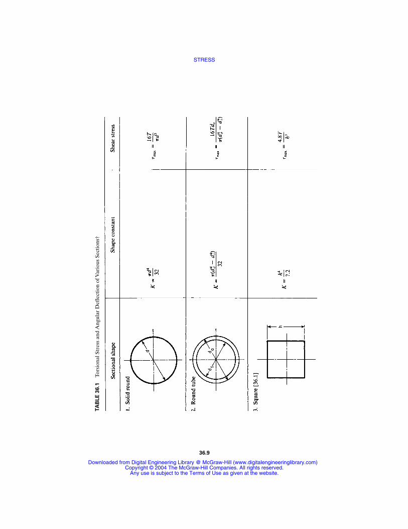
TA
BLE
36.1
Tors
iona
l Str
ess
and
Ang
ular
Def
lect
ion
of V
ario
us S
ecti
ons†
36.9
STRESS
Downloaded from Digital Engineering Library @ McGraw-Hill (www.digitalengineeringlibrary.com)Copyright © 2004 The McGraw-Hill Companies. All rights reserved.
Any use is subject to the Terms of Use as given at the website.
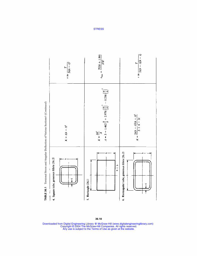
TA
BLE
36.1
Tors
iona
l Str
ess
and
Ang
ular
Def
lect
ion
of V
ario
us S
ecti
ons†
(C
ontin
ued)
36.10
STRESS
Downloaded from Digital Engineering Library @ McGraw-Hill (www.digitalengineeringlibrary.com)Copyright © 2004 The McGraw-Hill Companies. All rights reserved.
Any use is subject to the Terms of Use as given at the website.
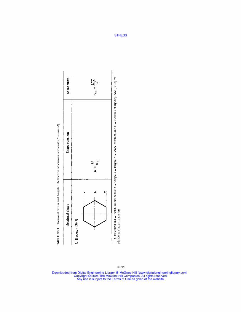
36.11
TA
BLE
36.1
Tors
iona
l Str
ess
and
Ang
ular
Def
lect
ion
of V
ario
us S
ecti
ons†
(C
ontin
ued)
STRESS
Downloaded from Digital Engineering Library @ McGraw-Hill (www.digitalengineeringlibrary.com)Copyright © 2004 The McGraw-Hill Companies. All rights reserved.
Any use is subject to the Terms of Use as given at the website.
36.3.2 Plastic Strain
It is important to observe that all the preceding relations are valid only when thematerial obeys Hooke’s law.
Some materials (see Sec. 32.9), when stressed in the plastic region, exhibit abehavior quite similar to that given by Eq. (36.11). For these materials, the appro-priate equation is
σ = Kεn (36.20)
where σ = true stressK = strength coefficientε = true plastic strainn = strain-strengthening exponent
The relations for the true stress and true strain are
σ = AFi
i ε = ln
ll
0
i (36.21)
where Ai and li are, respectively, the instantaneous values of the area and length of abar subjected to a load Fi. Note that the areas in Eqs. (36.9) are the original orunstressed areas; the subscript zero was omitted, as is customary. The relationsbetween true and engineering (nominal) stresses and strains are
σ = σ exp ε = ln( + 1) (36.22)
36.4 FLEXURE
Figure 36.4a shows a member loaded in flexure by a number of forces F and sup-ported by reactions R1 and R2 at the ends. At point C a distance x from R1, we canwrite
ΣMC = ΣMext + M = 0 (36.23)
where ΣMext = −xR1 + c1F1 + c2F2 and is called the external moment at section C. Theterm M, called the internal or resisting moment, is shown in its positive direction inboth parts b and c of Fig. 36.4. Figure 36.5 shows that a positive moment causes thetop surface of a beam to be concave.A negative moment causes the top surface to beconvex with one or both ends curved downward.
A similar relation can be defined for shear at section C:
ΣFy = ΣFext + V = 0 (36.24)
where ΣFext = R1 − F1 − F2 and is called the external shear force at C. The term V,called the internal shear force, is shown in its positive direction in both parts b and cof Fig. 36.4.
Figure 36.6 illustrates an application of these relations to obtain a set of shear andmoment diagrams.
36.12 CLASSICAL STRESS AND DEFORMATION ANALYSIS
STRESS
Downloaded from Digital Engineering Library @ McGraw-Hill (www.digitalengineeringlibrary.com)Copyright © 2004 The McGraw-Hill Companies. All rights reserved.
Any use is subject to the Terms of Use as given at the website.
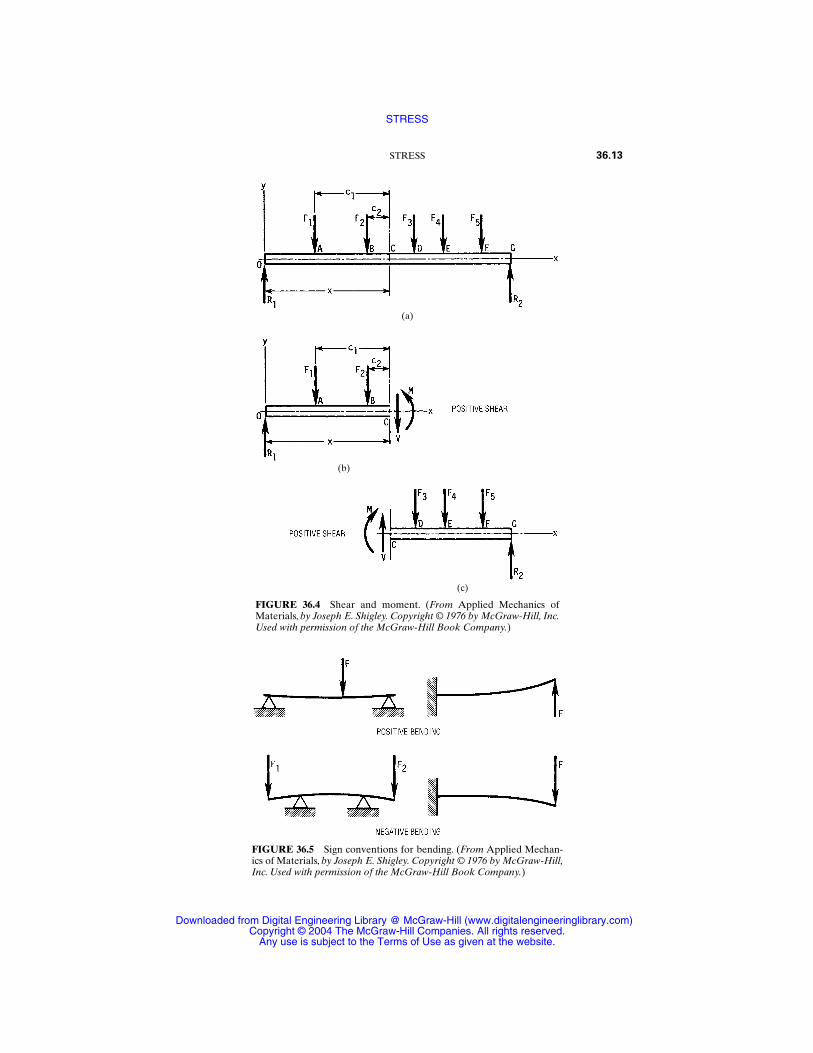
STRESS 36.13
FIGURE 36.4 Shear and moment. (From Applied Mechanics ofMaterials, by Joseph E. Shigley. Copyright © 1976 by McGraw-Hill, Inc.Used with permission of the McGraw-Hill Book Company.)
(c)
(b)
(a)
FIGURE 36.5 Sign conventions for bending. (From Applied Mechan-ics of Materials, by Joseph E. Shigley. Copyright © 1976 by McGraw-Hill,Inc. Used with permission of the McGraw-Hill Book Company.)
STRESS
Downloaded from Digital Engineering Library @ McGraw-Hill (www.digitalengineeringlibrary.com)Copyright © 2004 The McGraw-Hill Companies. All rights reserved.
Any use is subject to the Terms of Use as given at the website.
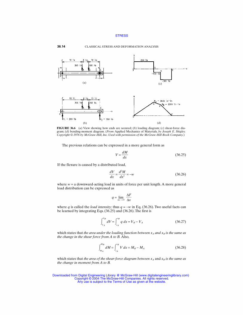
The previous relations can be expressed in a more general form as
V = ddMx (36.25)
If the flexure is caused by a distributed load,
ddVx =
dd
2
xM
2 = −w (36.26)
where w = a downward-acting load in units of force per unit length. A more generalload distribution can be expressed as
q = lim∆x → 0
∆∆
Fx
where q is called the load intensity; thus q = −w in Eq. (36.26). Two useful facts canbe learned by integrating Eqs. (36.25) and (36.26). The first is
VB
VA
dV = xB
xA
q dx = VB − VA (36.27)
which states that the area under the loading function between xA and xB is the same asthe change in the shear force from A to B. Also,
MB
MA
dM = xB
xA
V dx = MB − MA (36.28)
which states that the area of the shear-force diagram between xA and xB is the same asthe change in moment from A to B.
36.14 CLASSICAL STRESS AND DEFORMATION ANALYSIS
FIGURE 36.6 (a) View showing how ends are secured; (b) loading diagram; (c) shear-force dia-gram; (d) bending-moment diagram. (From Applied Mechanics of Materials, by Joseph E. Shigley.Copyright © 1976 by McGraw-Hill, Inc. Used with permission of the McGraw-Hill Book Company.)
(a) (c)
(b) (d)
STRESS
Downloaded from Digital Engineering Library @ McGraw-Hill (www.digitalengineeringlibrary.com)Copyright © 2004 The McGraw-Hill Companies. All rights reserved.
Any use is subject to the Terms of Use as given at the website.
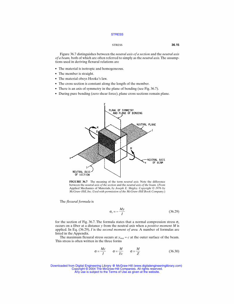
Figure 36.7 distinguishes between the neutral axis of a section and the neutral axisof a beam, both of which are often referred to simply as the neutral axis. The assump-tions used in deriving flexural relations are
The material is isotropic and homogeneous. The member is straight. The material obeys Hooke’s law. The cross section is constant along the length of the member. There is an axis of symmetry in the plane of bending (see Fig. 36.7). During pure bending (zero shear force), plane cross sections remain plane.
STRESS 36.15
FIGURE 36.7 The meaning of the term neutral axis. Note the differencebetween the neutral axis of the section and the neutral axis of the beam. (FromApplied Mechanics of Materials, by Joseph E. Shigley. Copyright © 1976 byMcGraw-Hill, Inc. Used with permission of the McGraw-Hill Book Company.)
The flexural formula is
σx = − M
Iy
(36.29)
for the section of Fig. 36.7. The formula states that a normal compression stress σx
occurs on a fiber at a distance y from the neutral axis when a positive moment M isapplied. In Eq. (36.29), I is the second moment of area. A number of formulas arelisted in the Appendix.
The maximum flexural stress occurs at ymax = c at the outer surface of the beam.This stress is often written in the three forms
σ = MIc
σ = σ = MZ
(36.30)MI/c
STRESS
Downloaded from Digital Engineering Library @ McGraw-Hill (www.digitalengineeringlibrary.com)Copyright © 2004 The McGraw-Hill Companies. All rights reserved.
Any use is subject to the Terms of Use as given at the website.
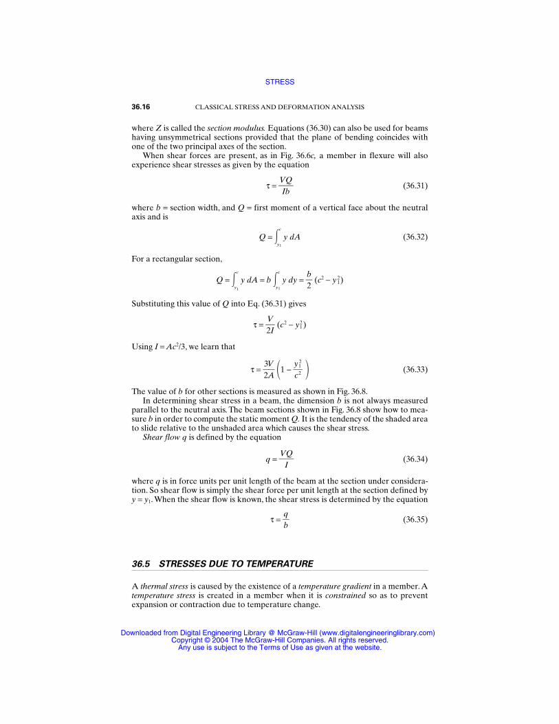
where Z is called the section modulus. Equations (36.30) can also be used for beamshaving unsymmetrical sections provided that the plane of bending coincides withone of the two principal axes of the section.
When shear forces are present, as in Fig. 36.6c, a member in flexure will alsoexperience shear stresses as given by the equation
τ = VIbQ (36.31)
where b = section width, and Q = first moment of a vertical face about the neutralaxis and is
Q = c
y1
y dA (36.32)
For a rectangular section,
Q = c
y1
y dA = b c
y1
y dy = b2
(c2 − y 12)
Substituting this value of Q into Eq. (36.31) gives
τ = 2VI (c2 − y1
2)
Using I = Ac2/3, we learn that
τ = 23AV 1 − (36.33)
The value of b for other sections is measured as shown in Fig. 36.8.In determining shear stress in a beam, the dimension b is not always measured
parallel to the neutral axis. The beam sections shown in Fig. 36.8 show how to mea-sure b in order to compute the static moment Q. It is the tendency of the shaded areato slide relative to the unshaded area which causes the shear stress.
Shear flow q is defined by the equation
q = V
IQ (36.34)
where q is in force units per unit length of the beam at the section under considera-tion. So shear flow is simply the shear force per unit length at the section defined byy = y1. When the shear flow is known, the shear stress is determined by the equation
τ = qb
(36.35)
36.5 STRESSES DUE TO TEMPERATURE
A thermal stress is caused by the existence of a temperature gradient in a member. Atemperature stress is created in a member when it is constrained so as to preventexpansion or contraction due to temperature change.
y12
c2
36.16 CLASSICAL STRESS AND DEFORMATION ANALYSIS
STRESS
Downloaded from Digital Engineering Library @ McGraw-Hill (www.digitalengineeringlibrary.com)Copyright © 2004 The McGraw-Hill Companies. All rights reserved.
Any use is subject to the Terms of Use as given at the website.
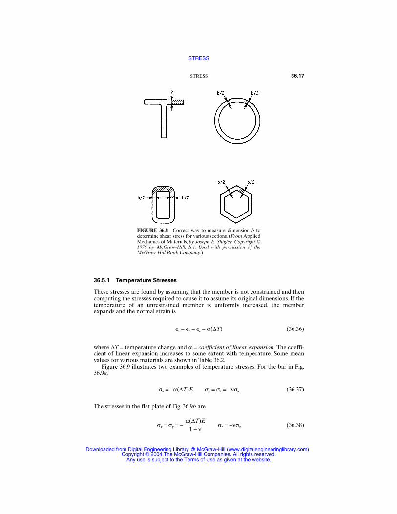
36.5.1 Temperature Stresses
These stresses are found by assuming that the member is not constrained and thencomputing the stresses required to cause it to assume its original dimensions. If thetemperature of an unrestrained member is uniformly increased, the memberexpands and the normal strain is
x = y = z = α(∆T) (36.36)
where ∆T = temperature change and α = coefficient of linear expansion. The coeffi-cient of linear expansion increases to some extent with temperature. Some meanvalues for various materials are shown in Table 36.2.
Figure 36.9 illustrates two examples of temperature stresses. For the bar in Fig.36.9a,
σx = −α(∆T)E σy = σz = −νσx (36.37)
The stresses in the flat plate of Fig. 36.9b are
σx = σy = − σz = −νσx (36.38)α(∆T)E
1 − ν
STRESS 36.17
FIGURE 36.8 Correct way to measure dimension b todetermine shear stress for various sections. (From AppliedMechanics of Materials, by Joseph E. Shigley. Copyright ©1976 by McGraw-Hill, Inc. Used with permission of theMcGraw-Hill Book Company.)
STRESS
Downloaded from Digital Engineering Library @ McGraw-Hill (www.digitalengineeringlibrary.com)Copyright © 2004 The McGraw-Hill Companies. All rights reserved.
Any use is subject to the Terms of Use as given at the website.
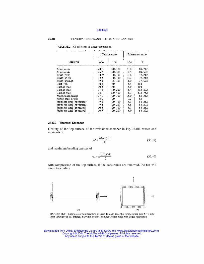
36.5.2 Thermal Stresses
Heating of the top surface of the restrained member in Fig. 36.10a causes endmoments of
M = (36.39)
and maximum bending stresses of
σx = ± (36.40)
with compression of the top surface. If the constraints are removed, the bar willcurve to a radius
α(∆T)E
2
α(∆T)EI
h
36.18 CLASSICAL STRESS AND DEFORMATION ANALYSIS
TABLE 36.2 Coefficients of Linear Expansion
FIGURE 36.9 Examples of temperature stresses. In each case the temperature rise ∆T is uni-form throughout. (a) Straight bar with ends restrained; (b) flat plate with edges restrained.
(a) (b)
STRESS
Downloaded from Digital Engineering Library @ McGraw-Hill (www.digitalengineeringlibrary.com)Copyright © 2004 The McGraw-Hill Companies. All rights reserved.
Any use is subject to the Terms of Use as given at the website.
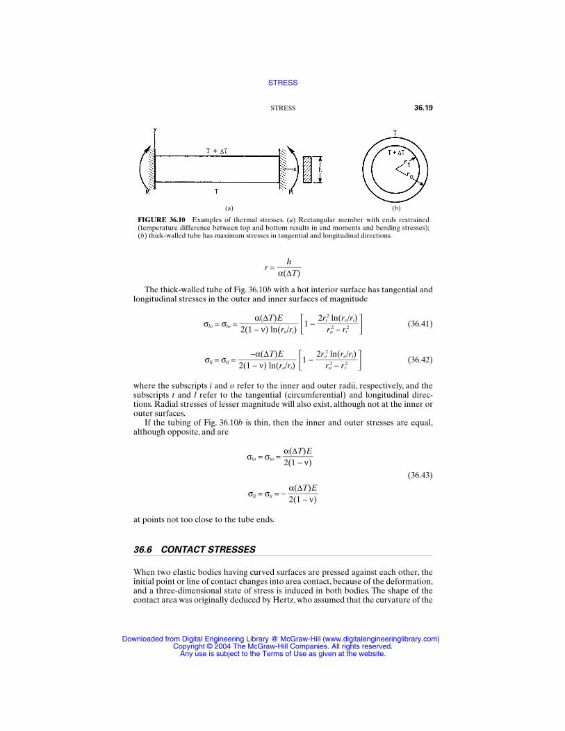
r =
The thick-walled tube of Fig. 36.10b with a hot interior surface has tangential andlongitudinal stresses in the outer and inner surfaces of magnitude
σlo = σto = 1 − (36.41)
σli = σti = 1 − (36.42)
where the subscripts i and o refer to the inner and outer radii, respectively, and thesubscripts t and l refer to the tangential (circumferential) and longitudinal direc-tions. Radial stresses of lesser magnitude will also exist, although not at the inner orouter surfaces.
If the tubing of Fig. 36.10b is thin, then the inner and outer stresses are equal,although opposite, and are
σlo = σto = α2(
(1∆T
−)νE)
σli = σti = − α2(
(1∆T
−)νE)
(36.43)
at points not too close to the tube ends.
36.6 CONTACT STRESSES
When two elastic bodies having curved surfaces are pressed against each other, theinitial point or line of contact changes into area contact, because of the deformation,and a three-dimensional state of stress is induced in both bodies. The shape of thecontact area was originally deduced by Hertz, who assumed that the curvature of the
2ro2 ln(ro/ri)
ro
2 − ri2
−α(∆T)E2(1 − ν) ln(ro/ri)
2ri2 ln(ro/ri)
ro
2 − ri2
α(∆T)E2(1 − ν) ln(ro/ri)
hα(∆T)
STRESS 36.19
FIGURE 36.10 Examples of thermal stresses. (a) Rectangular member with ends restrained(temperature difference between top and bottom results in end moments and bending stresses);(b) thick-walled tube has maximum stresses in tangential and longitudinal directions.
(a) (b)
STRESS
Downloaded from Digital Engineering Library @ McGraw-Hill (www.digitalengineeringlibrary.com)Copyright © 2004 The McGraw-Hill Companies. All rights reserved.
Any use is subject to the Terms of Use as given at the website.
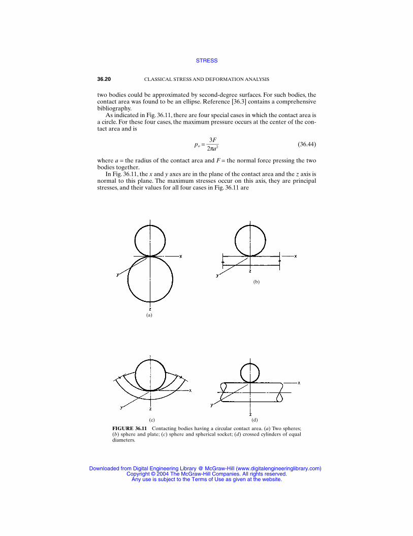
two bodies could be approximated by second-degree surfaces. For such bodies, thecontact area was found to be an ellipse. Reference [36.3] contains a comprehensivebibliography.
As indicated in Fig. 36.11, there are four special cases in which the contact area isa circle. For these four cases, the maximum pressure occurs at the center of the con-tact area and is
po = 23πFa2 (36.44)
where a = the radius of the contact area and F = the normal force pressing the twobodies together.
In Fig. 36.11, the x and y axes are in the plane of the contact area and the z axis isnormal to this plane. The maximum stresses occur on this axis, they are principalstresses, and their values for all four cases in Fig. 36.11 are
36.20 CLASSICAL STRESS AND DEFORMATION ANALYSIS
FIGURE 36.11 Contacting bodies having a circular contact area. (a) Two spheres;(b) sphere and plate; (c) sphere and spherical socket; (d) crossed cylinders of equaldiameters.
(c) (d)
(a)
(b)
STRESS
Downloaded from Digital Engineering Library @ McGraw-Hill (www.digitalengineeringlibrary.com)Copyright © 2004 The McGraw-Hill Companies. All rights reserved.
Any use is subject to the Terms of Use as given at the website.
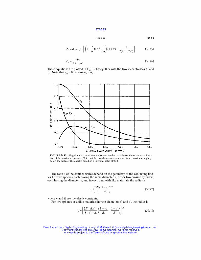
σx = σy = −po 1 − za
tan−1 z1/a (1 + ν) −
2(1 +1z2/a2) (36.45)
σz = 1 +
−pz2
o
/a2 (36.46)
These equations are plotted in Fig. 36.12 together with the two shear stresses τxz andτyz. Note that τxy = 0 because σx = σy.
STRESS 36.21
FIGURE 36.12 Magnitude of the stress components on the z axis below the surface as a func-tion of the maximum pressure. Note that the two shear-stress components are maximum slightlybelow the surface. The chart is based on a Poisson’s ratio of 0.30.
The radii a of the contact circles depend on the geometry of the contacting bod-ies. For two spheres, each having the same diameter d, or for two crossed cylinders,each having the diameter d, and in each case with like materials, the radius is
a = 3F
8d
1 −
Eν2
1/3
(36.47)
where ν and E are the elastic constants.For two spheres of unlike materials having diameters d1 and d2, the radius is
a = 38F
dd
1
1
+d
d2
2 +
1/3
(36.48)1 − ν2
2
E2
1 − ν12
E1
STRESS
Downloaded from Digital Engineering Library @ McGraw-Hill (www.digitalengineeringlibrary.com)Copyright © 2004 The McGraw-Hill Companies. All rights reserved.
Any use is subject to the Terms of Use as given at the website.
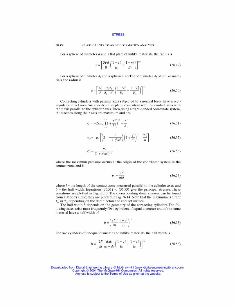
For a sphere of diameter d and a flat plate of unlike materials, the radius is
a = 3F
8d
+ 1/3
(36.49)
For a sphere of diameter d1 and a spherical socket of diameter d2 of unlike mate-rials, the radius is
a = 38F
dd
2
1
−d
d2
1 +
1/3
(36.50)
Contacting cylinders with parallel axes subjected to a normal force have a rect-angular contact area. We specify an xy plane coincident with the contact area withthe x axis parallel to the cylinder axes.Then, using a right-handed coordinate system,the stresses along the z axis are maximum and are
σx = −2νpo 1 + bz2
21/2
− bz
(36.51)
σy = −po 2 − 1 +
1z2/b2 1 +
bz2
21/2
− 2bz (36.52)
σz = (36.53)
where the maximum pressure occurs at the origin of the coordinate system in thecontact zone and is
po = π2bFl
(36.54)
where l = the length of the contact zone measured parallel to the cylinder axes, andb = the half width. Equations (36.51) to (36.53) give the principal stresses. Theseequations are plotted in Fig. 36.13. The corresponding shear stresses can be foundfrom a Mohr’s circle; they are plotted in Fig. 36.14. Note that the maximum is eitherτxz or τyz depending on the depth below the contact surface.
The half width b depends on the geometry of the contacting cylinders. The fol-lowing cases arise most frequently: Two cylinders of equal diameter and of the samematerial have a half width of
b = 2πFld
1 −
Eν2
1/2
(36.55)
For two cylinders of unequal diameter and unlike materials, the half width is
b = 2πFl
dd
1
1
+d
d2
2 1 E
−1
ν12
+ 1
E−
2
ν22
1/2
(36.56)
−po(1 + z2/b2)1/2
1 − ν22
E2
1 − ν12
E1
1 − ν22
E2
1 − ν12
E1
36.22 CLASSICAL STRESS AND DEFORMATION ANALYSIS
STRESS
Downloaded from Digital Engineering Library @ McGraw-Hill (www.digitalengineeringlibrary.com)Copyright © 2004 The McGraw-Hill Companies. All rights reserved.
Any use is subject to the Terms of Use as given at the website.
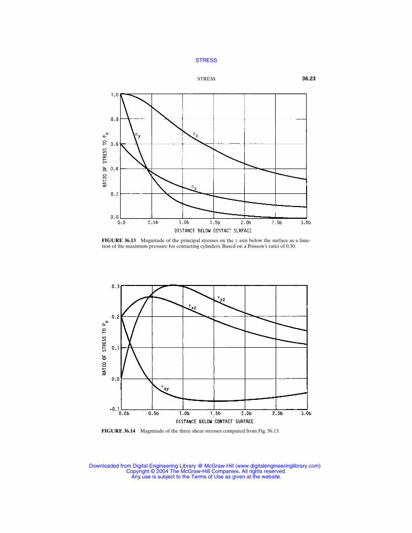
STRESS 36.23
FIGURE 36.13 Magnitude of the principal stresses on the z axis below the surface as a func-tion of the maximum pressure for contacting cylinders. Based on a Poisson’s ratio of 0.30.
FIGURE 36.14 Magnitude of the three shear stresses computed from Fig. 36.13.
STRESS
Downloaded from Digital Engineering Library @ McGraw-Hill (www.digitalengineeringlibrary.com)Copyright © 2004 The McGraw-Hill Companies. All rights reserved.
Any use is subject to the Terms of Use as given at the website.
For a cylinder of diameter d in contact with a flat plate of unlike material, the resultis
b = 2πFld
1 E−
1
ν12
+ 1
E−
2
ν22
1/2
(36.57)
The half width for a cylinder of diameter d1 pressing against a cylindrical socketof diameter d2 of unlike material is
b = 2πFl
dd
2
1
−d
d2
1 1 E
−1
ν12
+ 1
E−
2
ν22
1/2
(36.58)
REFERENCES
36.1 F. R. Shanley, Strength of Materials, McGraw-Hill, New York, 1957, p. 509.
36.2 W. C. Young, Roark’s Formulas for Stress and Strain, 6th ed., McGraw-Hill, 1989, p.348–359.
36.3 J. L. Lubkin, “Contact Problems,” in W. Flugge (ed.), Handbook of Engineering Mechan-ics, McGraw-Hill, New York, 1962, pp. 42-10 to 42-12.
36.24 CLASSICAL STRESS AND DEFORMATION ANALYSIS
STRESS
Downloaded from Digital Engineering Library @ McGraw-Hill (www.digitalengineeringlibrary.com)Copyright © 2004 The McGraw-Hill Companies. All rights reserved.
Any use is subject to the Terms of Use as given at the website.

CHAPTER 37DEFLECTION
Joseph E. ShigleyProfessor Emeritus
The University of MichiganAnn Arbor, Michigan
Charles R. Mischke, Ph.D., P.E.Professor Emeritus of Mechanical Engineering
Iowa State UniversityAmes, Iowa
37.1 STIFFNESS OR SPRING RATE / 37.2
37.2 DEFLECTION DUE TO BENDING / 37.3
37.3 PROPERTIES OF BEAMS / 37.3
37.4 ANALYSIS OF FRAMES / 37.3
GLOSSARY OF SYMBOLS
a Dimension
A Area
b Dimension
C Constant
D, d Diameter
E Young’s modulus
F Force
G Shear modulus
I Second moment of area
J Second polar moment of area
k Spring rate
K Constant
Length
M Moment
N Number
37.1
Source: STANDARD HANDBOOK OF MACHINE DESIGN
Downloaded from Digital Engineering Library @ McGraw-Hill (www.digitalengineeringlibrary.com)Copyright © 2004 The McGraw-Hill Companies. All rights reserved.
Any use is subject to the Terms of Use as given at the website.
q Unit loadQ Fictitious forceR Support reactionT TorqueU Strain energyV Shear forcew Unit weightW Total weightx Coordinatey Coordinateδ Deflectionθ Slope, torsional deflection
37.1 STIFFNESS OR SPRING RATE
The spring rate (also called stiffness or scale) of a body or ensemble of bodies isdefined as the partial derivative of force (torque) with respect to colinear displace-ment (rotation). For a helical tension or compression spring,
F = thus k = = (37.1)
where D = mean coil diameterd = wire diameterN = number of active turns
In a round bar subject to torsion,
T = G
Jθ thus k =
∂∂Tθ =
GJ
(37.2)
and the tensile force in an elongating bar of any cross section is
F = A
Eδ thus k =
∂∂Fδ =
AE (37.3)
If k is constant, as in these cases, then displacement is said to be linear with respectto force (torque). For contacting bodies with all four radii of curvature finite, theapproach of the bodies is proportional to load to the two-thirds power, making thespring rate proportional to load to the one-third power. In hydrodynamic film bear-ings, the partial derivative would be evaluated numerically by dividing a smallchange in load by the displacement in the direction of the load.
d4G8D3N
∂F∂y
d4Gy8D3N
37.2 CLASSICAL STRESS AND DEFORMATION ANALYSIS
DEFLECTION
Downloaded from Digital Engineering Library @ McGraw-Hill (www.digitalengineeringlibrary.com)Copyright © 2004 The McGraw-Hill Companies. All rights reserved.
Any use is subject to the Terms of Use as given at the website.
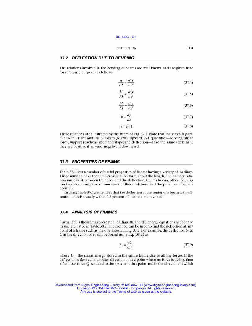
37.2 DEFLECTION DUE TO BENDING
The relations involved in the bending of beams are well known and are given herefor reference purposes as follows:
= (37.4)
= (37.5)
= (37.6)
θ = (37.7)
y = f(x) (37.8)
These relations are illustrated by the beam of Fig. 37.1. Note that the x axis is posi-tive to the right and the y axis is positive upward. All quantities—loading, shearforce, support reactions, moment, slope, and deflection—have the same sense as y;they are positive if upward, negative if downward.
37.3 PROPERTIES OF BEAMS
Table 37.1 lists a number of useful properties of beams having a variety of loadings.These must all have the same cross section throughout the length, and a linear rela-tion must exist between the force and the deflection. Beams having other loadingscan be solved using two or more sets of these relations and the principle of super-position.
In using Table 37.1, remember that the deflection at the center of a beam with off-center loads is usually within 2.5 percent of the maximum value.
37.4 ANALYSIS OF FRAMES
Castigliano’s theorem is presented in Chap. 38, and the energy equations needed forits use are listed in Table 38.2. The method can be used to find the deflection at anypoint of a frame such as the one shown in Fig. 37.2. For example, the deflection δC atC in the direction of F2 can be found using Eq. (38.2) as
δC = (37.9)
where U = the strain energy stored in the entire frame due to all the forces. If thedeflection is desired in another direction or at a point where no force is acting, thena fictitious force Q is added to the system at that point and in the direction in which
∂U∂F2
dydx
d2ydx2
MEI
d 3ydx3
VEI
d 4ydx4
qEI
DEFLECTION 37.3
DEFLECTION
Downloaded from Digital Engineering Library @ McGraw-Hill (www.digitalengineeringlibrary.com)Copyright © 2004 The McGraw-Hill Companies. All rights reserved.
Any use is subject to the Terms of Use as given at the website.
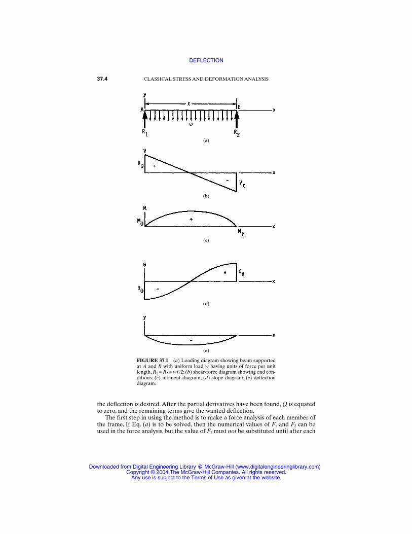
the deflection is desired.After the partial derivatives have been found, Q is equatedto zero, and the remaining terms give the wanted deflection.
The first step in using the method is to make a force analysis of each member ofthe frame. If Eq. (a) is to be solved, then the numerical values of F1 and F2 can beused in the force analysis, but the value of F2 must not be substituted until after each
37.4 CLASSICAL STRESS AND DEFORMATION ANALYSIS
FIGURE 37.1 (a) Loading diagram showing beam supportedat A and B with uniform load w having units of force per unitlength, R1 = R2 = w/2; (b) shear-force diagram showing end con-ditions; (c) moment diagram; (d) slope diagram; (e) deflectiondiagram.
(a)
(b)
(c)
(d)
(e)
DEFLECTION
Downloaded from Digital Engineering Library @ McGraw-Hill (www.digitalengineeringlibrary.com)Copyright © 2004 The McGraw-Hill Companies. All rights reserved.
Any use is subject to the Terms of Use as given at the website.
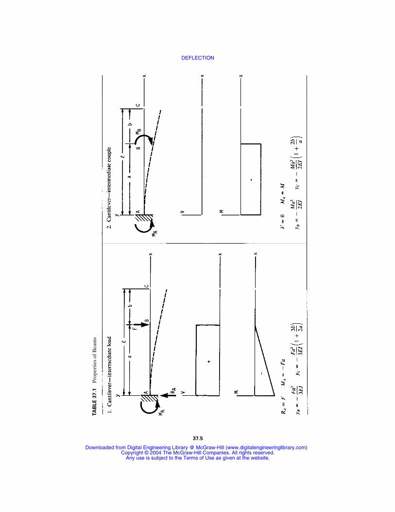
TA
BLE
37.1
Pro
pert
ies
of B
eam
s
37.5
DEFLECTION
Downloaded from Digital Engineering Library @ McGraw-Hill (www.digitalengineeringlibrary.com)Copyright © 2004 The McGraw-Hill Companies. All rights reserved.
Any use is subject to the Terms of Use as given at the website.
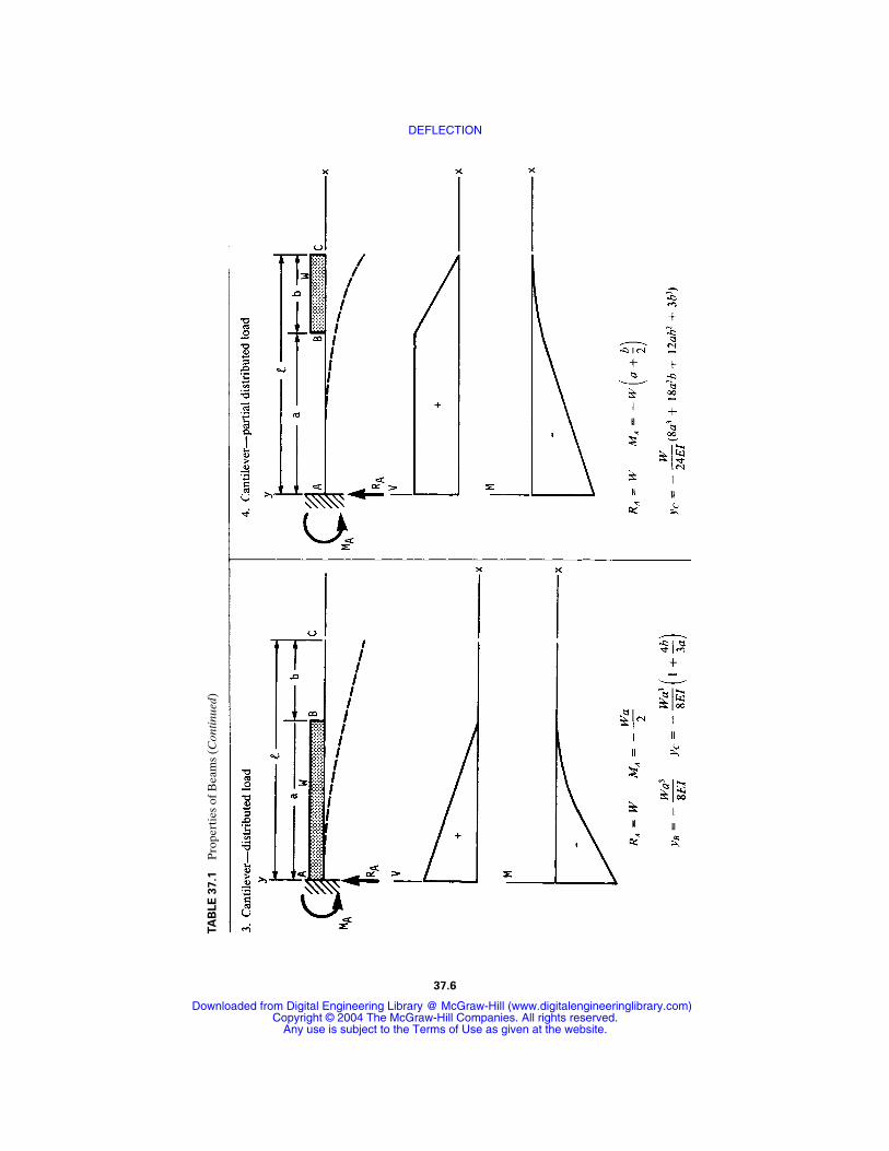
37.6
TA
BLE
37.1
Pro
pert
ies
of B
eam
s (C
ontin
ued)
DEFLECTION
Downloaded from Digital Engineering Library @ McGraw-Hill (www.digitalengineeringlibrary.com)Copyright © 2004 The McGraw-Hill Companies. All rights reserved.
Any use is subject to the Terms of Use as given at the website.
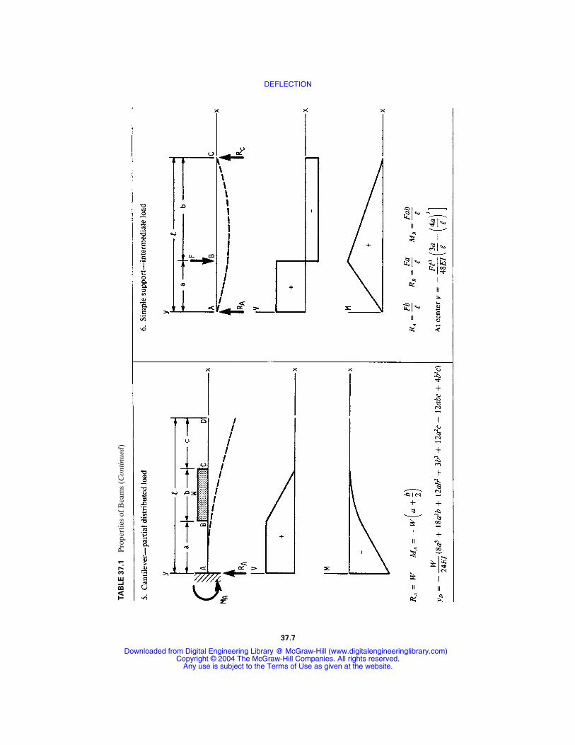
37.7
TA
BLE
37.1
Pro
pert
ies
of B
eam
s (C
ontin
ued)
DEFLECTION
Downloaded from Digital Engineering Library @ McGraw-Hill (www.digitalengineeringlibrary.com)Copyright © 2004 The McGraw-Hill Companies. All rights reserved.
Any use is subject to the Terms of Use as given at the website.
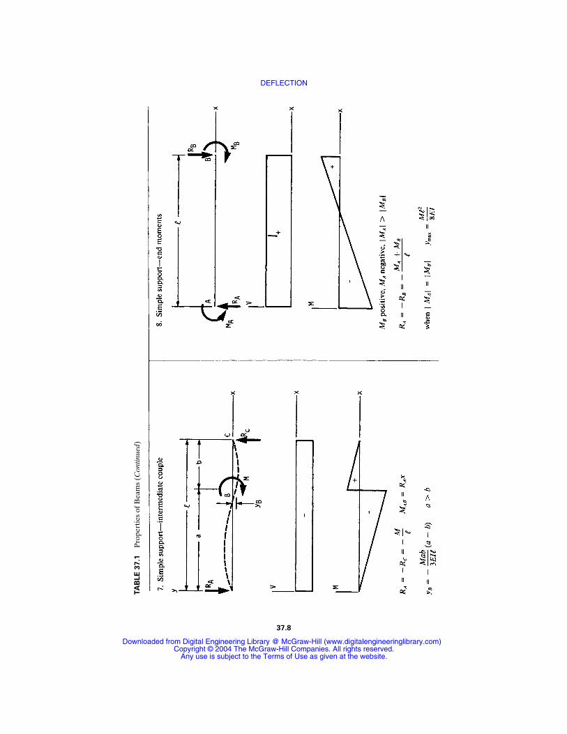
37.8
TA
BLE
37.1
Pro
pert
ies
of B
eam
s (C
ontin
ued)
DEFLECTION
Downloaded from Digital Engineering Library @ McGraw-Hill (www.digitalengineeringlibrary.com)Copyright © 2004 The McGraw-Hill Companies. All rights reserved.
Any use is subject to the Terms of Use as given at the website.
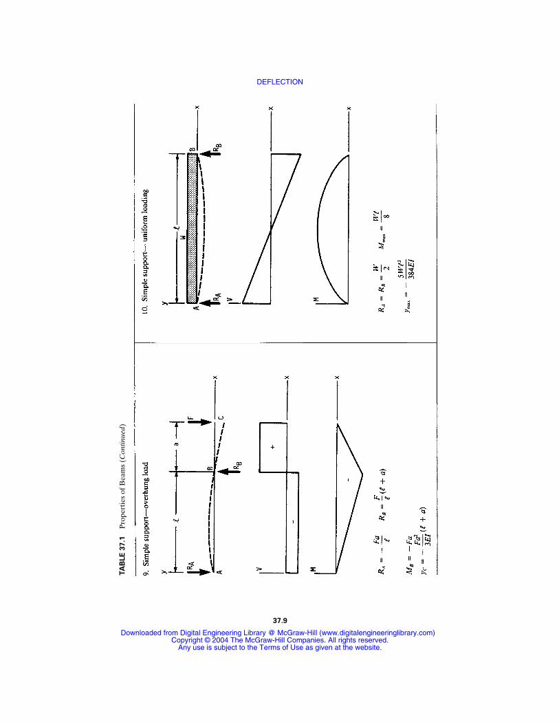
37.9
TA
BLE
37.1
Pro
pert
ies
of B
eam
s (C
ontin
ued)
DEFLECTION
Downloaded from Digital Engineering Library @ McGraw-Hill (www.digitalengineeringlibrary.com)Copyright © 2004 The McGraw-Hill Companies. All rights reserved.
Any use is subject to the Terms of Use as given at the website.
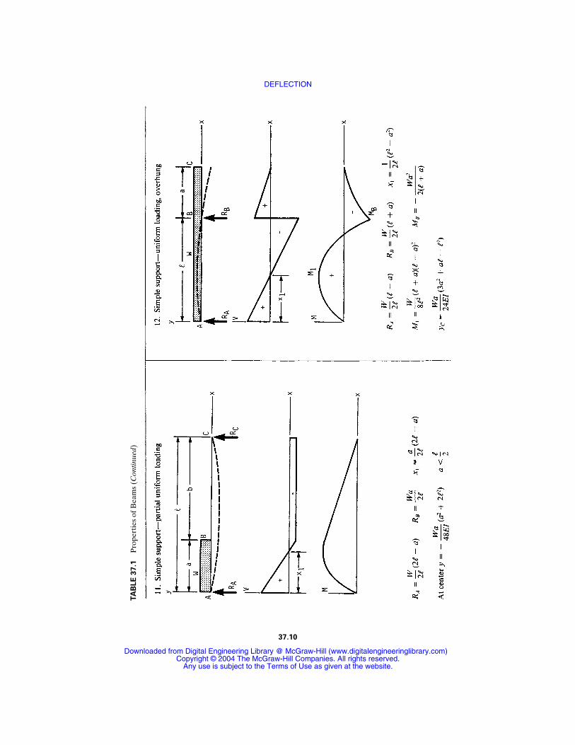
37.10
TA
BLE
37.1
Pro
pert
ies
of B
eam
s (C
ontin
ued)
DEFLECTION
Downloaded from Digital Engineering Library @ McGraw-Hill (www.digitalengineeringlibrary.com)Copyright © 2004 The McGraw-Hill Companies. All rights reserved.
Any use is subject to the Terms of Use as given at the website.
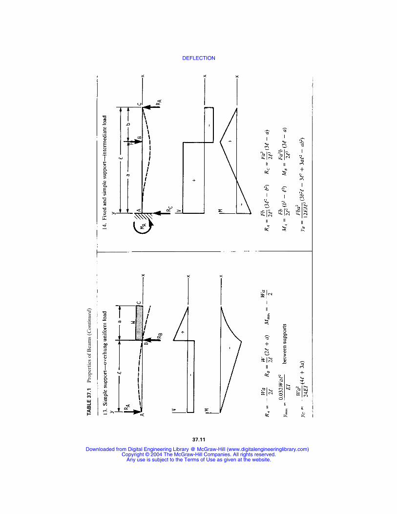
37.11
TA
BLE
37.1
Pro
pert
ies
of B
eam
s (C
ontin
ued)
DEFLECTION
Downloaded from Digital Engineering Library @ McGraw-Hill (www.digitalengineeringlibrary.com)Copyright © 2004 The McGraw-Hill Companies. All rights reserved.
Any use is subject to the Terms of Use as given at the website.
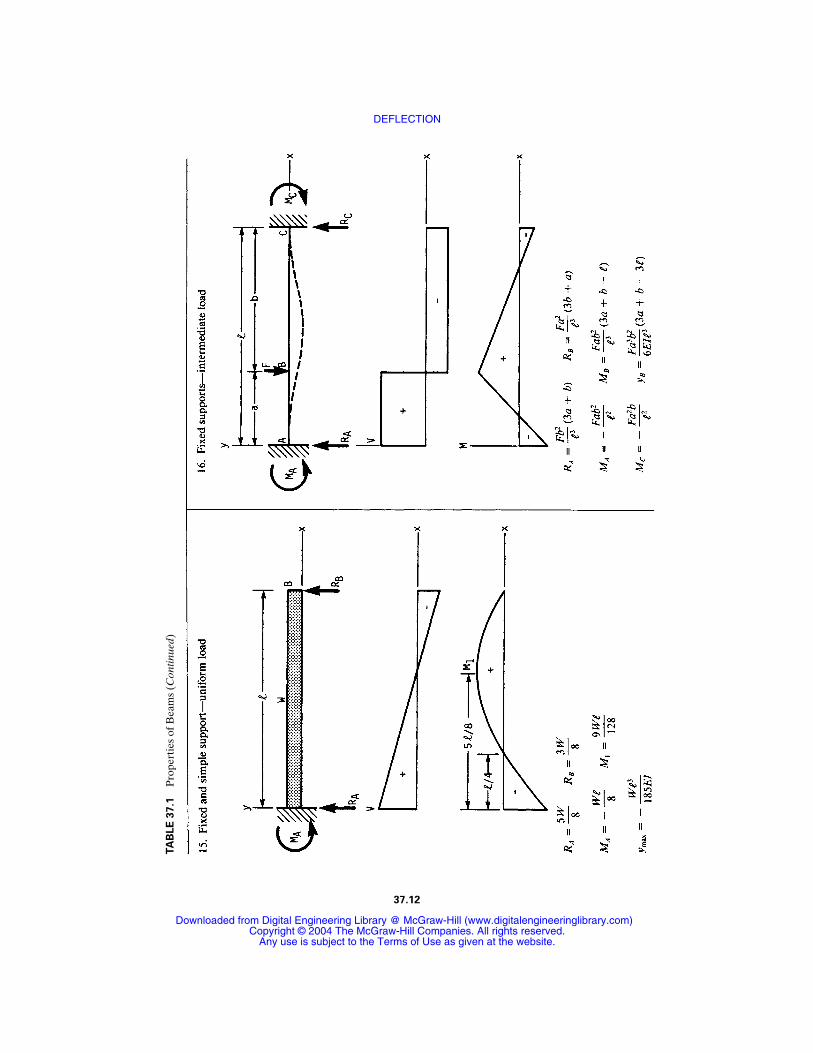
37.12
TA
BLE
37.1
Pro
pert
ies
of B
eam
s (C
ontin
ued)
DEFLECTION
Downloaded from Digital Engineering Library @ McGraw-Hill (www.digitalengineeringlibrary.com)Copyright © 2004 The McGraw-Hill Companies. All rights reserved.
Any use is subject to the Terms of Use as given at the website.
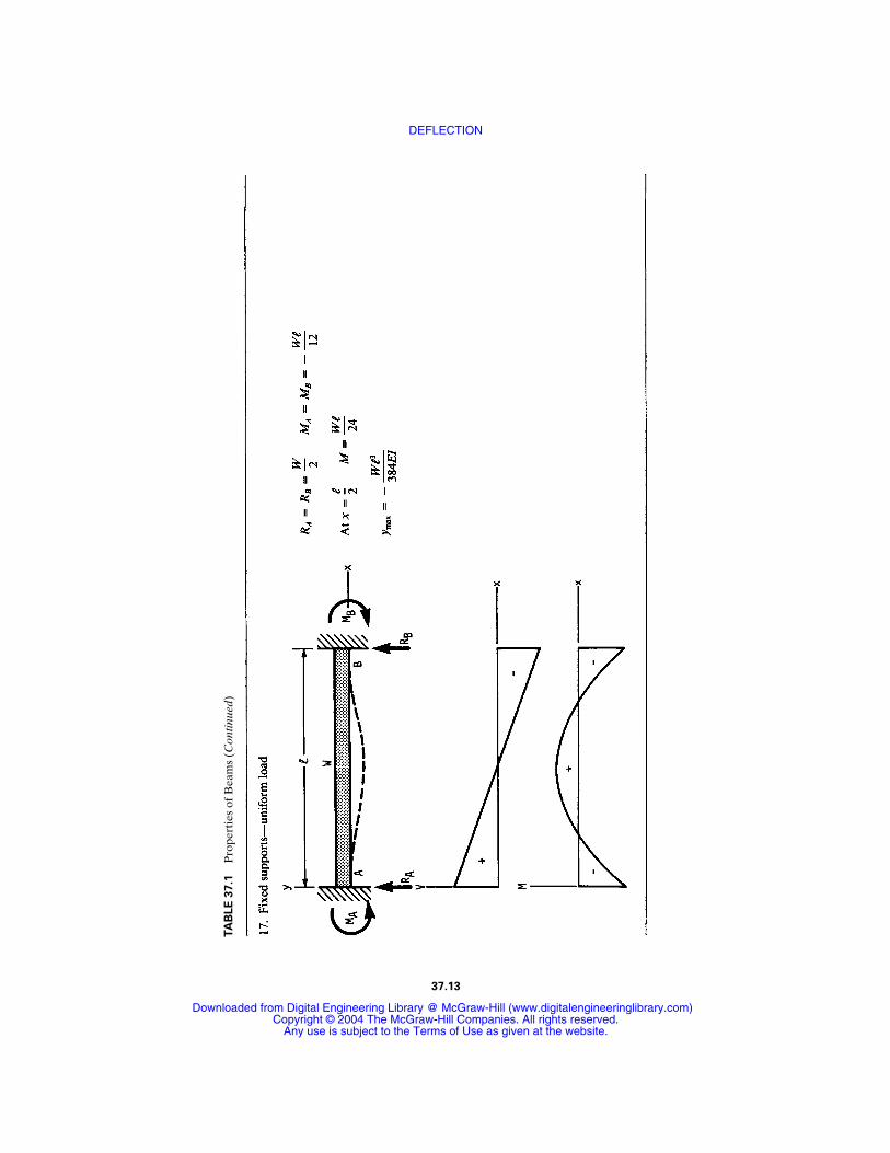
37.13
TA
BLE
37.1
Pro
pert
ies
of B
eam
s (C
ontin
ued)
DEFLECTION
Downloaded from Digital Engineering Library @ McGraw-Hill (www.digitalengineeringlibrary.com)Copyright © 2004 The McGraw-Hill Companies. All rights reserved.
Any use is subject to the Terms of Use as given at the website.
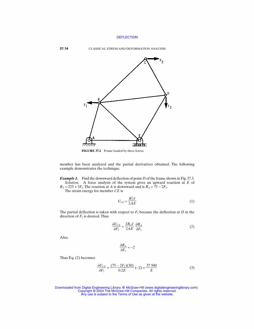
member has been analyzed and the partial derivatives obtained. The followingexample demonstrates the technique.
Example 1. Find the downward deflection of point D of the frame shown in Fig. 37.3.Solution. A force analysis of the system gives an upward reaction at E of
RE = 225 + 3F2. The reaction at A is downward and is RA = 75 − 2F2.The strain energy for member CE is
UCE = (1)
The partial deflection is taken with respect to F2 because the deflection at D in thedirection of F2 is desired. Thus
= (2)
Also,
= −2
Thus Eq. (2) becomes
= (−2) = (3)37 500
E(75 − 2F2)(30)
0.2E∂UCE∂F2
∂RA∂F2
∂RA∂F2
2RA2AE
∂UCE∂F2
RA2
2AE
37.14 CLASSICAL STRESS AND DEFORMATION ANALYSIS
FIGURE 37.2 Frame loaded by three forces.
DEFLECTION
Downloaded from Digital Engineering Library @ McGraw-Hill (www.digitalengineeringlibrary.com)Copyright © 2004 The McGraw-Hill Companies. All rights reserved.
Any use is subject to the Terms of Use as given at the website.
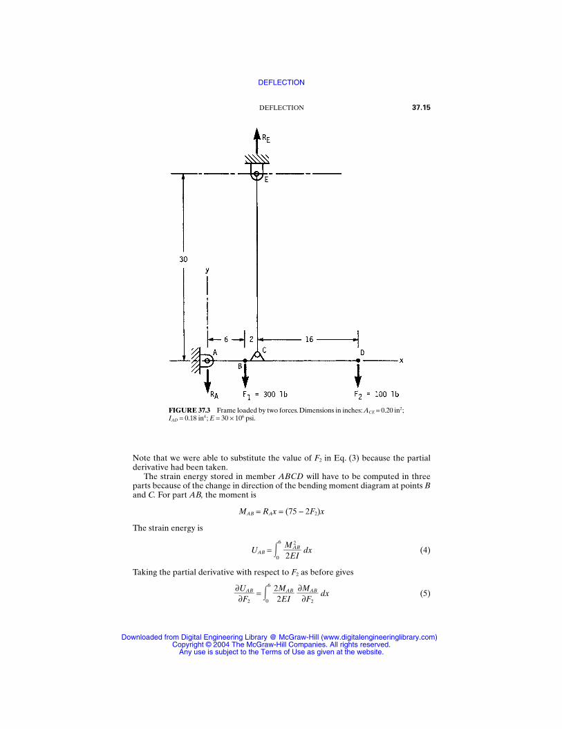
Note that we were able to substitute the value of F2 in Eq. (3) because the partialderivative had been taken.
The strain energy stored in member ABCD will have to be computed in threeparts because of the change in direction of the bending moment diagram at points Band C. For part AB, the moment is
MAB = RAx = (75 − 2F2)x
The strain energy is
UAB = 6
0dx (4)
Taking the partial derivative with respect to F2 as before gives
= 6
0dx (5)
∂MAB∂F2
2MAB2EI
∂UAB∂F2
M 2AB
2EI
DEFLECTION 37.15
FIGURE 37.3 Frame loaded by two forces. Dimensions in inches: ACE = 0.20 in2;IAD = 0.18 in4; E = 30 × 106 psi.
DEFLECTION
Downloaded from Digital Engineering Library @ McGraw-Hill (www.digitalengineeringlibrary.com)Copyright © 2004 The McGraw-Hill Companies. All rights reserved.
Any use is subject to the Terms of Use as given at the website.
But
= −2x (6)
Therefore, Eq. (5) may be written
= E1I 6
0x(75 − 2F2)(−2x) dx
= 6
0250x2 dx = (7)
where the value of F2 again has been substituted after taking the partial derivative.For section BC, we have
MBC = RAx − F1(x − 6) = 1800 − 225x − 2F2x
= −2x
= 8
6dx
= E1I 8
6(1800 − 225x − 2F2x)(−2x) dx
= 8
6(−3600x + 850x2) dx =
Finally, section CD yields
MCD = −(24 − x)F2 = −(24 − x)
= 24
8dx
= E1I 24
8F2(24 − x)2 dx
= 24
8(57 600 − 4800x + 100x2) dx
=
Then
yD = + + +
= (37 500 + 100 000 + 145 926 + 758 519)
= 0.0347 in (when rounded)
130(10)6
∂UCD∂F2
∂UBC∂F2
∂UAB∂F2
∂UCE∂F2
758 519
E
10.18E
∂MCD∂F2
2MCD2EI
∂UCD∂F2
∂MCD∂F2
145 926
E1
0.18E
∂MBC∂F2
2MBC2EI
∂UBC∂F2
∂MBC∂F2
100 000
E1
0.18E
∂UAB∂F2
∂MAB∂F2
37.16 CLASSICAL STRESS AND DEFORMATION ANALYSIS
DEFLECTION
Downloaded from Digital Engineering Library @ McGraw-Hill (www.digitalengineeringlibrary.com)Copyright © 2004 The McGraw-Hill Companies. All rights reserved.
Any use is subject to the Terms of Use as given at the website.
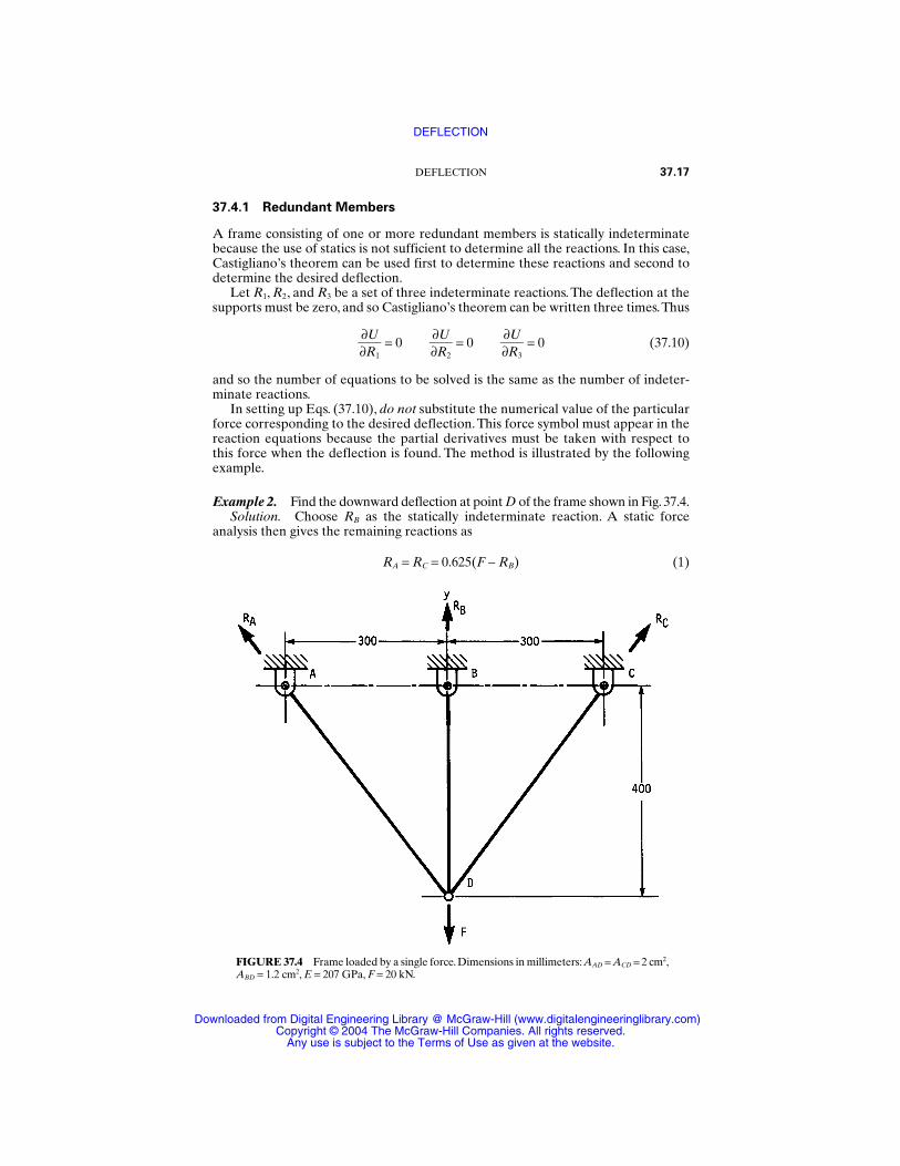
37.4.1 Redundant Members
A frame consisting of one or more redundant members is statically indeterminatebecause the use of statics is not sufficient to determine all the reactions. In this case,Castigliano’s theorem can be used first to determine these reactions and second todetermine the desired deflection.
Let R1, R2, and R3 be a set of three indeterminate reactions. The deflection at thesupports must be zero, and so Castigliano’s theorem can be written three times.Thus
= 0 = 0 = 0 (37.10)
and so the number of equations to be solved is the same as the number of indeter-minate reactions.
In setting up Eqs. (37.10), do not substitute the numerical value of the particularforce corresponding to the desired deflection. This force symbol must appear in thereaction equations because the partial derivatives must be taken with respect tothis force when the deflection is found. The method is illustrated by the followingexample.
Example 2. Find the downward deflection at point D of the frame shown in Fig. 37.4.Solution. Choose RB as the statically indeterminate reaction. A static force
analysis then gives the remaining reactions as
RA = RC = 0.625(F − RB) (1)
∂U∂R3
∂U∂R2
∂U∂R1
DEFLECTION 37.17
FIGURE 37.4 Frame loaded by a single force. Dimensions in millimeters: AAD = ACD = 2 cm2,ABD = 1.2 cm2, E = 207 GPa, F = 20 kN.
DEFLECTION
Downloaded from Digital Engineering Library @ McGraw-Hill (www.digitalengineeringlibrary.com)Copyright © 2004 The McGraw-Hill Companies. All rights reserved.
Any use is subject to the Terms of Use as given at the website.

The frame consists only of tension members, so the strain energy in each member is
UAD = UDC = UBD = (2)
Using Eq. (37.10), we now write
0 = = + (3)
Equation (1) gives ∂RA/∂RB = −0.625. Also, ∂RB/∂RB = 1. Substituting numerical val-ues in Eq. (3), except for F, gives
+ = 0 (4)
Solving gives RB = 0.369F. Therefore, from Eq. (1), RA = RC = 0.394F. This completesthe solution of the case of the redundant member. The next problem is to find thedeflection at D.
Using Eq. (2), again we write
yD = = + (5)
For use in this equation, we note that ∂RA/∂F = 0.394 and ∂RB/∂F = 0.369. Havingtaken the derivatives, we can now substitute the numerical value of F. Thus Eq. (5)becomes†
∂RB∂F
RBBDABDE
∂RA∂F
2RAADAADE
∂U∂F
RB(400)(1)
1.2(207)2(0.625)(F − RB)(500)(−0.625)
2(207)
∂RB∂RB
RBBDABDE
∂RA∂RB
2RAADAADE
∂U∂RB
RB2 BD
2ABDERA
2 AD2AADE
37.18 CLASSICAL STRESS AND DEFORMATION ANALYSIS
† In general, when using metric quantities, prefixed units are chosen so as to produce number strings ofnot more than four members. Thus some preferred units in SI are MPa (N/mm2) for stress, GPa for modulusof elasticity, mm for length, and, say, cm4 for second moment of area.
People are sometimes confused when they encounter an equation containing a number of mixed units.Suppose we wish to solve a deflection equation of the form
y =
where F = 1.30 kN, = 300 mm, d = 2.5 cm, and E = 207 GPa. Form the equation into two parts, the first con-taining the numbers and the second containing the prefixes.This converts everything to base units, includingthe result. Thus,
y =
Now compute the numerical value of the first part and substitute the prefix values in the second. This gives
y = (29.48 × 10³) = 29.48 × 10⁻⁴ m
= 2.948 mm
Note that we multiplied the result by 103 mm/m to get the answer in millimeters.When this approach is usedwith Eq. (5), it is found that the result must be multiplied by (10)−2 to get y in millimeters.
103(10−3)3
(10−2)4(109)
(kilo)(milli)3
(centi)4(giga)
64(1.30)(300)3
3π(2.5)4(207)
64F3
3πd4E
DEFLECTION
Downloaded from Digital Engineering Library @ McGraw-Hill (www.digitalengineeringlibrary.com)Copyright © 2004 The McGraw-Hill Companies. All rights reserved.
Any use is subject to the Terms of Use as given at the website.

DEFLECTION 37.19
yD = + 10−2
= 0.119 mm
If care is taken to refrain from substituting numerical values for reactions or forcesuntil after partial derivatives are taken, Castigliano’s theorem is applicable to stati-cally indeterminate frames containing redundant members.
[0.369(20)](400)(0.369)
1.2(207)2[0.394(20)](500)(0.394)
2(207)
DEFLECTION
Downloaded from Digital Engineering Library @ McGraw-Hill (www.digitalengineeringlibrary.com)Copyright © 2004 The McGraw-Hill Companies. All rights reserved.
Any use is subject to the Terms of Use as given at the website.

DEFLECTION
Downloaded from Digital Engineering Library @ McGraw-Hill (www.digitalengineeringlibrary.com)Copyright © 2004 The McGraw-Hill Companies. All rights reserved.
Any use is subject to the Terms of Use as given at the website.

CHAPTER 38CURVED BEAMS AND RINGS
Joseph E. ShigleyProfessor Emeritus
The University of MichiganAnn Arbor, Michigan
38.1 BENDING IN THE PLANE OF CURVATURE / 38.2
38.2 CASTIGLIANO’S THEOREM / 38.2
38.3 RING SEGMENTS WITH ONE SUPPORT / 38.3
38.4 RINGS WITH SIMPLE SUPPORTS / 38.10
38.5 RING SEGMENTS WITH FIXED ENDS / 38.15
REFERENCES / 38.22
NOTATION
A Area, or a constantB ConstantC ConstantE Modulus of elasticitye EccentricityF ForceG Modulus of rigidityI Second moment of area (Table A.1)K Shape constant (Table 36.1), or second polar moment of areaM Bending momentP Reduced loadQ Fictitious forceR Force reactionr Ring radiusr Centroidal ring radiusT Torsional momentU Strain energyV Shear forceW Resultant of a distributed loadw Unit distributed loadX Constant
38.1
Source: STANDARD HANDBOOK OF MACHINE DESIGN
Downloaded from Digital Engineering Library @ McGraw-Hill (www.digitalengineeringlibrary.com)Copyright © 2004 The McGraw-Hill Companies. All rights reserved.
Any use is subject to the Terms of Use as given at the website.
Y Constanty DeflectionZ Constantγ Load angleφ Span angle, or slopeσ Normal stressθ Angular coordinate or displacement
Methods of computing the stresses in curved beams for a variety of cross sectionsare included in this chapter. Rings and ring segments loaded normal to the plane ofthe ring are analyzed for a variety of loads and span angles, and formulas are givenfor bending moment, torsional moment, and deflection.
38.1 BENDING IN THE PLANE OF CURVATURE
The distribution of stress in a curved member subjected to a bending moment in theplane of curvature is hyperbolic ([38.1], [38.2]) and is given by the equation
σ = (38.1)
where r = radius to centroidal axisy = distance from neutral axise = shift in neutral axis due to curvature (as noted in Table 38.1)
The moment M is computed about the centroidal axis, not the neutral axis. Themaximum stresses, which occur on the extreme fibers, may be computed using theformulas of Table 38.1.
In most cases, the bending moment is due to forces acting to one side of the sec-tion. In such cases, be sure to add the resulting axial stress to the maximum stressesobtained using Table 38.1.
38.2 CASTIGLIANO’S THEOREM
A complex structure loaded by any combination of forces, moments, and torques canbe analyzed for deflections by using the elastic energy stored in the various compo-nents of the structure [38.1]. The method consists of finding the total strain energystored in the system by all the various loads. Then the displacement correspondingto a particular force is obtained by taking the partial derivative of the total energywith respect to that force. This procedure is called Castigliano’s theorem. Generalexpressions may be written as
yi = ∂∂UFi θi =
∂∂TU
i φi =
∂∂MU
i (38.2)
where U = strain energy stored in structureyi = displacement of point of application of force Fi in the direction of Fi
MyAe(r − e − y)
38.2 CLASSICAL STRESS AND DEFORMATION ANALYSIS
CURVED BEAMS AND RINGS
Downloaded from Digital Engineering Library @ McGraw-Hill (www.digitalengineeringlibrary.com)Copyright © 2004 The McGraw-Hill Companies. All rights reserved.
Any use is subject to the Terms of Use as given at the website.
θi = angular displacement at Ti
φi = slope or angular displacement at moment Mi
If a displacement is desired at a point on the structure where no force or momentexists, then a fictitious force or moment is placed there. When the expression for thecorresponding displacement is developed, the fictitious force or moment is equatedto zero, and the remaining terms give the deflection at the point where the fictitiousload had been placed.
Castigliano’s method can also be used to find the reactions in indeterminatestructures. The procedure is simply to substitute the unknown reaction in Eq. (38.2)and use zero for the corresponding deflection. The resulting expression then yieldsthe value of the unknown reaction.
It is important to remember that the displacement-force relation must be linear.Otherwise, the theorem is not valid.
Table 38.2 summarizes strain-energy relations.
38.3 RING SEGMENTS WITH ONE SUPPORT
Figure 38.1 shows a cantilevered ring segment fixed at C. The force F causes bend-ing, torsion, and direct shear.The moments and torques at the fixed end C and at anysection B are shown in Table 38.3.The shear at C is RC = F. Stresses in the ring can becomputed using the formulas of Chap. 36.
To obtain the deflection at end A, we use Castigliano’s theorem. Neglectingdirect shear and noting from Fig. 38.1b that l = r dθ, we determine the strain energyfrom Table 38.2 to be
U = φ
0M
2
2
Er
Idθ
+ φ
0T2
2
Gr
Kdθ (38.3)
Then the deflection y at A and in the direction of F is computed from
y = ∂θUF =
ErI φ
0M
∂∂MF dθ +
GrK φ
0T
∂∂TF dθ (38.4)
The terms for this relation are shown in Table 38.3. It is convenient to arrange thesolution in the form
y = F2r3
EA
I +
GBK (38.5)
where the coefficients A and B are related only to the span angle.These are listed inTable 38.3.
Figure 38.2a shows another cantilevered ring segment, loaded now by a dis-tributed load. The resultant load is W = wrφ; a shear reaction R = W acts upward atthe fixed end C, in addition to the moment and torque reactions shown in Table 38.3.
A force W = wrθ acts at the centroid of segment AB in Fig. 38.2b. The centroidalradius is
r = 2r sinθ
(θ/2) (38.6)
CURVED BEAMS AND RINGS 38.3
CURVED BEAMS AND RINGS
Downloaded from Digital Engineering Library @ McGraw-Hill (www.digitalengineeringlibrary.com)Copyright © 2004 The McGraw-Hill Companies. All rights reserved.
Any use is subject to the Terms of Use as given at the website.
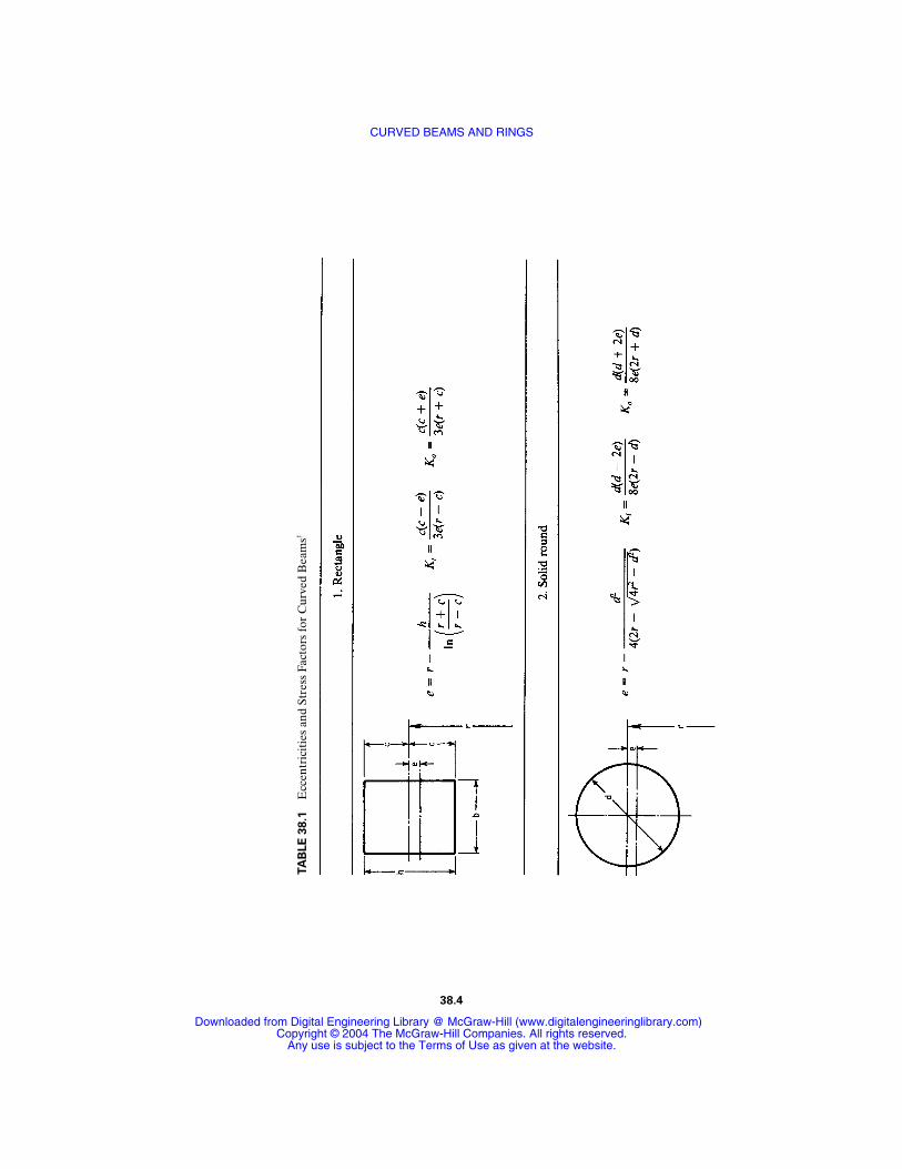
38.4
TA
BLE
38.1
Ecc
entr
icit
ies
and
Stre
ss F
acto
rs fo
r C
urve
d B
eam
s†
CURVED BEAMS AND RINGS
Downloaded from Digital Engineering Library @ McGraw-Hill (www.digitalengineeringlibrary.com)Copyright © 2004 The McGraw-Hill Companies. All rights reserved.
Any use is subject to the Terms of Use as given at the website.
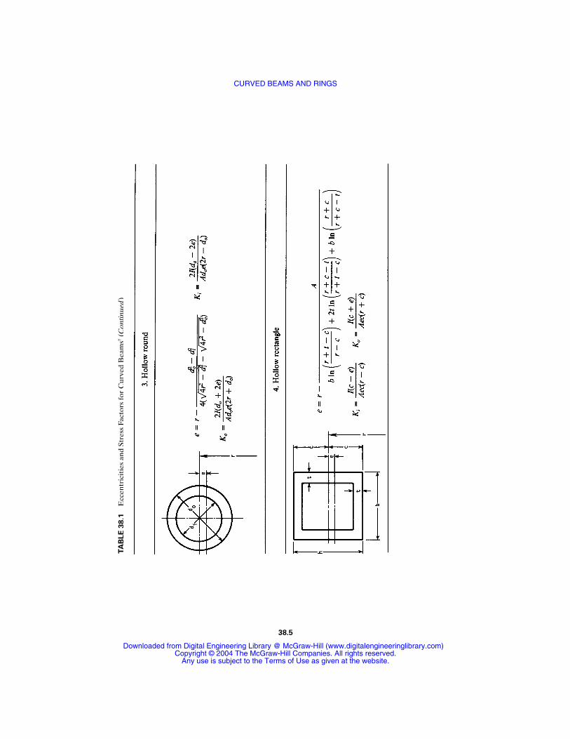
38.5
TA
BLE
38.1
Ecc
entr
icit
ies
and
Stre
ss F
acto
rs fo
r C
urve
d B
eam
s†(C
ontin
ued
)
CURVED BEAMS AND RINGS
Downloaded from Digital Engineering Library @ McGraw-Hill (www.digitalengineeringlibrary.com)Copyright © 2004 The McGraw-Hill Companies. All rights reserved.
Any use is subject to the Terms of Use as given at the website.
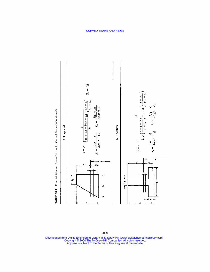
38.6
TA
BLE
38.1
Ecc
entr
icit
ies
and
Stre
ss F
acto
rs fo
r C
urve
d B
eam
s†(C
ontin
ued
)
CURVED BEAMS AND RINGS
Downloaded from Digital Engineering Library @ McGraw-Hill (www.digitalengineeringlibrary.com)Copyright © 2004 The McGraw-Hill Companies. All rights reserved.
Any use is subject to the Terms of Use as given at the website.
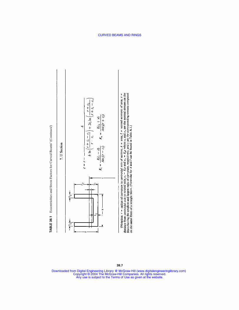
38.7
TA
BLE
38.1
Ecc
entr
icit
ies
and
Stre
ss F
acto
rs fo
r C
urve
d B
eam
s†(C
ontin
ued
)
CURVED BEAMS AND RINGS
Downloaded from Digital Engineering Library @ McGraw-Hill (www.digitalengineeringlibrary.com)Copyright © 2004 The McGraw-Hill Companies. All rights reserved.
Any use is subject to the Terms of Use as given at the website.
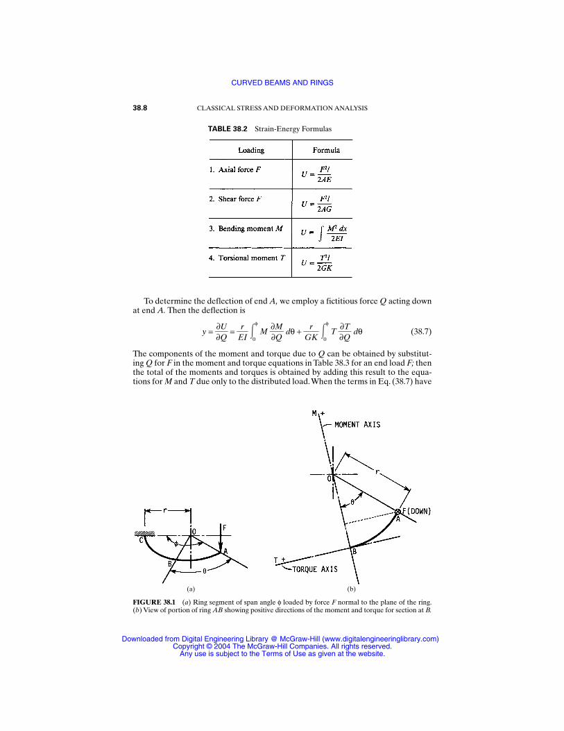
To determine the deflection of end A, we employ a fictitious force Q acting downat end A. Then the deflection is
y = ∂∂QU =
ErI φ
0M
∂∂MQ dθ +
GrK φ
0T
∂∂QT dθ (38.7)
The components of the moment and torque due to Q can be obtained by substitut-ing Q for F in the moment and torque equations in Table 38.3 for an end load F; thenthe total of the moments and torques is obtained by adding this result to the equa-tions for M and T due only to the distributed load.When the terms in Eq. (38.7) have
38.8 CLASSICAL STRESS AND DEFORMATION ANALYSIS
TABLE 38.2 Strain-Energy Formulas
(a) (b)
FIGURE 38.1 (a) Ring segment of span angle φ loaded by force F normal to the plane of the ring.(b) View of portion of ring AB showing positive directions of the moment and torque for section at B.
CURVED BEAMS AND RINGS
Downloaded from Digital Engineering Library @ McGraw-Hill (www.digitalengineeringlibrary.com)Copyright © 2004 The McGraw-Hill Companies. All rights reserved.
Any use is subject to the Terms of Use as given at the website.
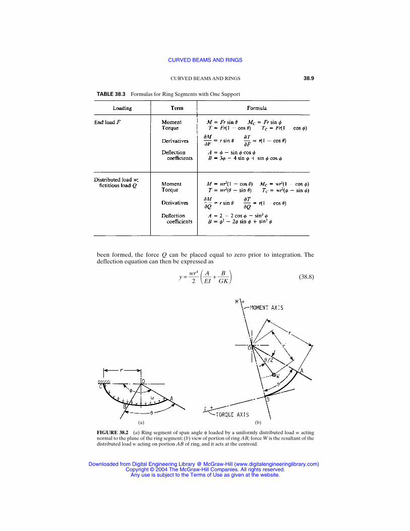
been formed, the force Q can be placed equal to zero prior to integration. Thedeflection equation can then be expressed as
y = w2r4
EA
I +
GBK (38.8)
CURVED BEAMS AND RINGS 38.9
TABLE 38.3 Formulas for Ring Segments with One Support
(a) (b)
FIGURE 38.2 (a) Ring segment of span angle φ loaded by a uniformly distributed load w actingnormal to the plane of the ring segment; (b) view of portion of ring AB; force W is the resultant of thedistributed load w acting on portion AB of ring, and it acts at the centroid.
CURVED BEAMS AND RINGS
Downloaded from Digital Engineering Library @ McGraw-Hill (www.digitalengineeringlibrary.com)Copyright © 2004 The McGraw-Hill Companies. All rights reserved.
Any use is subject to the Terms of Use as given at the website.
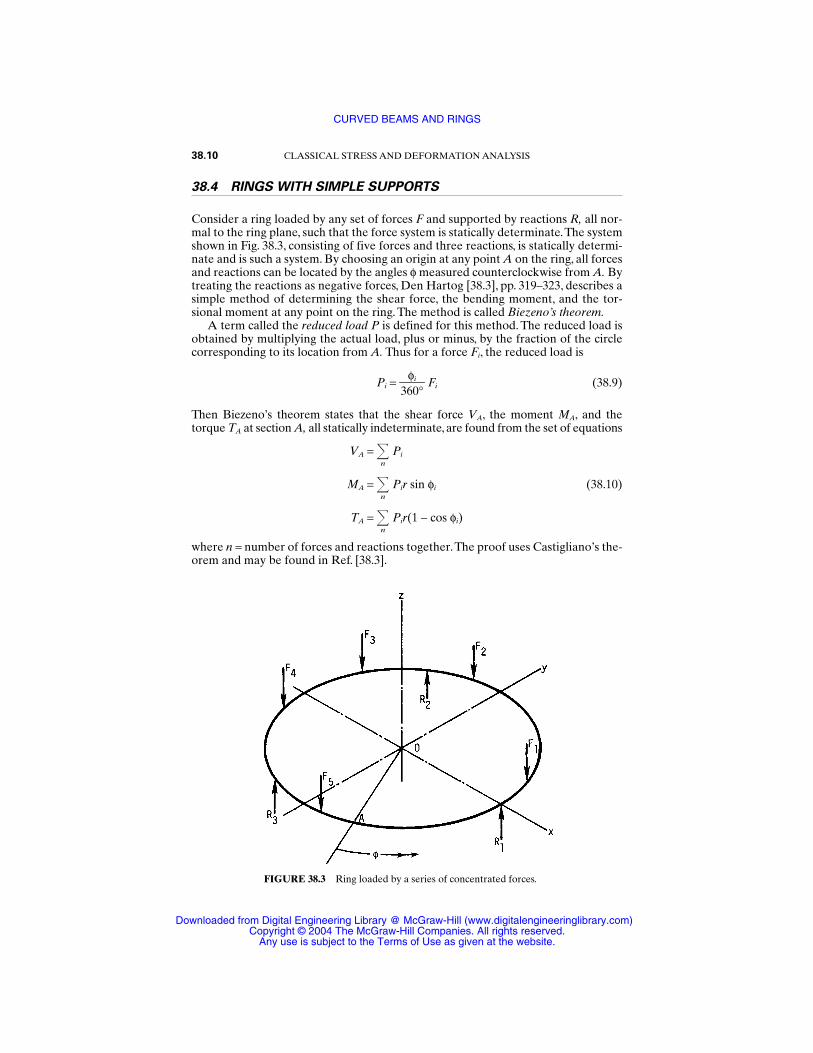
38.4 RINGS WITH SIMPLE SUPPORTS
Consider a ring loaded by any set of forces F and supported by reactions R, all nor-mal to the ring plane, such that the force system is statically determinate.The systemshown in Fig. 38.3, consisting of five forces and three reactions, is statically determi-nate and is such a system. By choosing an origin at any point A on the ring, all forcesand reactions can be located by the angles φ measured counterclockwise from A. Bytreating the reactions as negative forces, Den Hartog [38.3], pp. 319–323, describes asimple method of determining the shear force, the bending moment, and the tor-sional moment at any point on the ring. The method is called Biezeno’s theorem.
A term called the reduced load P is defined for this method. The reduced load isobtained by multiplying the actual load, plus or minus, by the fraction of the circlecorresponding to its location from A. Thus for a force Fi, the reduced load is
Pi = 36
φ0i
° Fi (38.9)
Then Biezeno’s theorem states that the shear force VA, the moment MA, and thetorque TA at section A, all statically indeterminate, are found from the set of equations
VA = n
Pi
MA = n
Pir sin φi (38.10)
TA = n
Pir(1 − cos φi)
where n = number of forces and reactions together.The proof uses Castigliano’s the-orem and may be found in Ref. [38.3].
38.10 CLASSICAL STRESS AND DEFORMATION ANALYSIS
FIGURE 38.3 Ring loaded by a series of concentrated forces.
CURVED BEAMS AND RINGS
Downloaded from Digital Engineering Library @ McGraw-Hill (www.digitalengineeringlibrary.com)Copyright © 2004 The McGraw-Hill Companies. All rights reserved.
Any use is subject to the Terms of Use as given at the website.
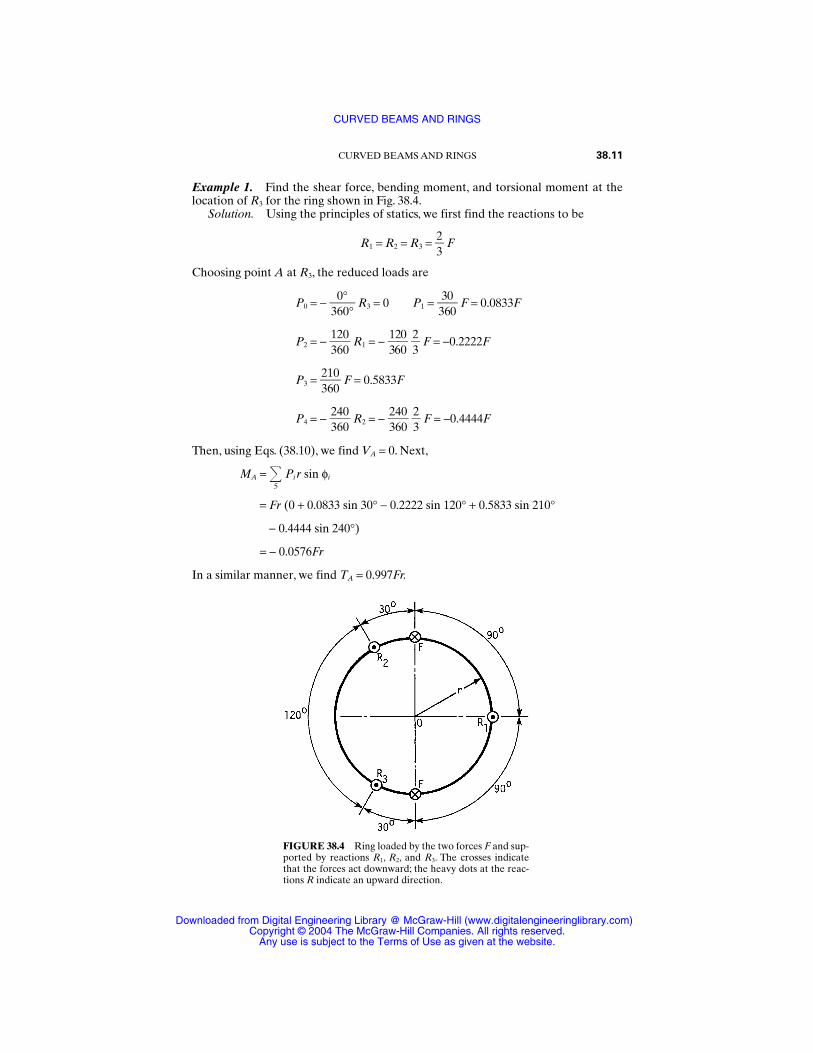
Example 1. Find the shear force, bending moment, and torsional moment at thelocation of R3 for the ring shown in Fig. 38.4.
Solution. Using the principles of statics, we first find the reactions to be
R1 = R2 = R3 = 23
F
Choosing point A at R3, the reduced loads are
P0 = − 306°0° R3 = 0 P1 =
33600
F = 0.0833F
P2 = − 132600
R1 = − 132600
23
F = −0.2222F
P3 = 231600
F = 0.5833F
P4 = − 234600
R2 = − 234600
23
F = −0.4444F
Then, using Eqs. (38.10), we find VA = 0. Next,
MA = 5
Pir sin φi
= Fr (0 + 0.0833 sin 30° − 0.2222 sin 120° + 0.5833 sin 210°
− 0.4444 sin 240°)
= − 0.0576Fr
In a similar manner, we find TA = 0.997Fr.
CURVED BEAMS AND RINGS 38.11
FIGURE 38.4 Ring loaded by the two forces F and sup-ported by reactions R1, R2, and R3. The crosses indicatethat the forces act downward; the heavy dots at the reac-tions R indicate an upward direction.
CURVED BEAMS AND RINGS
Downloaded from Digital Engineering Library @ McGraw-Hill (www.digitalengineeringlibrary.com)Copyright © 2004 The McGraw-Hill Companies. All rights reserved.
Any use is subject to the Terms of Use as given at the website.
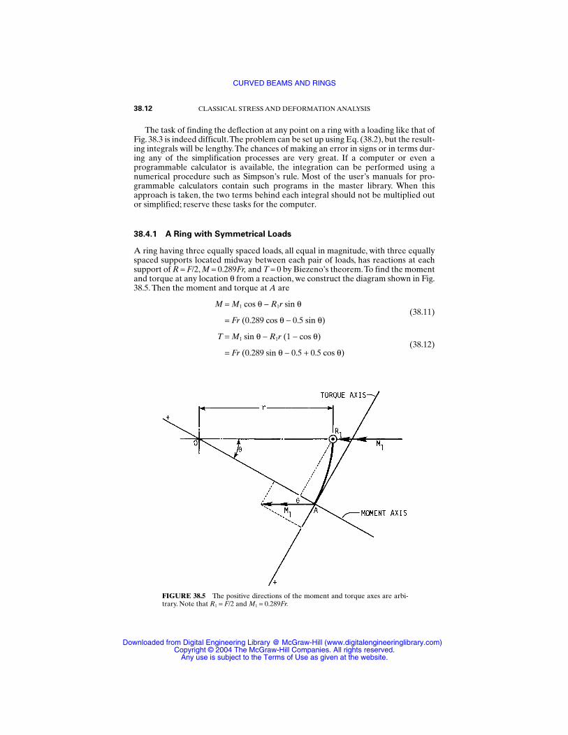
The task of finding the deflection at any point on a ring with a loading like that ofFig. 38.3 is indeed difficult.The problem can be set up using Eq. (38.2), but the result-ing integrals will be lengthy.The chances of making an error in signs or in terms dur-ing any of the simplification processes are very great. If a computer or even aprogrammable calculator is available, the integration can be performed using anumerical procedure such as Simpson’s rule. Most of the user’s manuals for pro-grammable calculators contain such programs in the master library. When thisapproach is taken, the two terms behind each integral should not be multiplied outor simplified; reserve these tasks for the computer.
38.4.1 A Ring with Symmetrical Loads
A ring having three equally spaced loads, all equal in magnitude, with three equallyspaced supports located midway between each pair of loads, has reactions at eachsupport of R = F/2, M = 0.289Fr, and T = 0 by Biezeno’s theorem.To find the momentand torque at any location θ from a reaction, we construct the diagram shown in Fig.38.5. Then the moment and torque at A are
M = M1 cos θ − R1r sin θ
= Fr (0.289 cos θ − 0.5 sin θ)(38.11)
T = M1 sin θ − R1r (1 − cos θ)
= Fr (0.289 sin θ − 0.5 + 0.5 cos θ)(38.12)
38.12 CLASSICAL STRESS AND DEFORMATION ANALYSIS
FIGURE 38.5 The positive directions of the moment and torque axes are arbi-trary. Note that R1 = F/2 and M1 = 0.289Fr.
CURVED BEAMS AND RINGS
Downloaded from Digital Engineering Library @ McGraw-Hill (www.digitalengineeringlibrary.com)Copyright © 2004 The McGraw-Hill Companies. All rights reserved.
Any use is subject to the Terms of Use as given at the website.
Neglecting direct shear, the strain energy stored in the ring between any two sup-ports is, from Table 38.2,
U = 2 π/3
0M
2
2
Er
Idθ
+ 2 π/3
0T2
2
Gr
Kdθ (38.13)
Castigliano’s theorem states that the deflection at the load F is
y = ∂∂UF =
E2r
I π/3
0M
∂∂MF dθ +
G2Kr π/3
0T
∂∂TF dθ (38.14)
From Eqs. (38.11) and (38.12), we find
∂∂MF = r(0.289 cos θ − 0.5 sin θ)
∂∂TF = r(0.289 sin θ − 0.5 + 0.5 cos θ)
When these are substituted into Eq. (38.14), we get
y = F2r3
EA
I +
GBK (38.15)
which is the same as Eq. (38.5). The constants are
A = 4 π/3
0(0.289 cos θ − 0.5 sin θ)2 dθ
B = 4 π/3
0(0.289 sin θ − 0.5 + 0.5 cos θ)2 dθ
(38.16)
These equations can be integrated directly or by a computer using Simpson’s rule. Ifyour integration is rusty, use the computer.The results are A = 0.1208 and B = 0.0134.
38.4.2 Distributed Loading
The ring segment in Fig. 38.6 is subjected to a distributed load w per unit circumfer-ence and is supported by the vertical reactions R1 and R2 and the moment reactionsM1 and M2. The zero-torque reactions mean that the ring is free to turn at A and B.The resultant of the distributed load is W = wrφ; it acts at the centroid:
r = 2r sinφ
(φ/2) (38.17)
By symmetry, the force reactions are R1 = R2 = W/2 = wrφ/2. Summing momentsabout an axis through BO gives
ΣM(BO) = −M2 + Wr sin φ2
− M1 cos (π − φ) − wr
2
2φ sin φ = 0
Since M1 and M2 are equal, this equation can be solved to give
CURVED BEAMS AND RINGS 38.13
CURVED BEAMS AND RINGS
Downloaded from Digital Engineering Library @ McGraw-Hill (www.digitalengineeringlibrary.com)Copyright © 2004 The McGraw-Hill Companies. All rights reserved.
Any use is subject to the Terms of Use as given at the website.
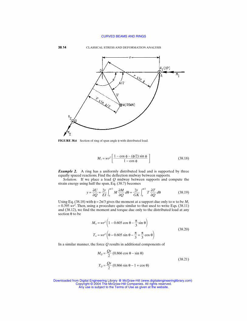
M1 = wr2 (38.18)
Example 2. A ring has a uniformly distributed load and is supported by threeequally spaced reactions. Find the deflection midway between supports.
Solution. If we place a load Q midway between supports and compute thestrain energy using half the span, Eq. (38.7) becomes
y = ∂∂QU =
E2r
I φ/2
0M
∂∂MQ dθ +
G2Kr φ/2
0T
∂∂QT dθ (38.19)
Using Eq. (38.18) with φ = 2π/3 gives the moment at a support due only to w to be M1
= 0.395 wr2. Then, using a procedure quite similar to that used to write Eqs. (38.11)and (38.12), we find the moment and torque due only to the distributed load at anysection θ to be
Mw = wr2 1 − 0.605 cos θ − π3
sin θTw = wr2 θ − 0.605 sin θ −
π3
+ π3
cos θ(38.20)
In a similar manner, the force Q results in additional components of
MQ = Q2r
(0.866 cos θ − sin θ)
TQ = Q2r
(0.866 sin θ − 1 + cos θ)
(38.21)
1 − cos φ − (φ/2) sin φ
1 − cos φ
38.14 CLASSICAL STRESS AND DEFORMATION ANALYSIS
FIGURE 38.6 Section of ring of span angle φ with distributed load.
CURVED BEAMS AND RINGS
Downloaded from Digital Engineering Library @ McGraw-Hill (www.digitalengineeringlibrary.com)Copyright © 2004 The McGraw-Hill Companies. All rights reserved.
Any use is subject to the Terms of Use as given at the website.
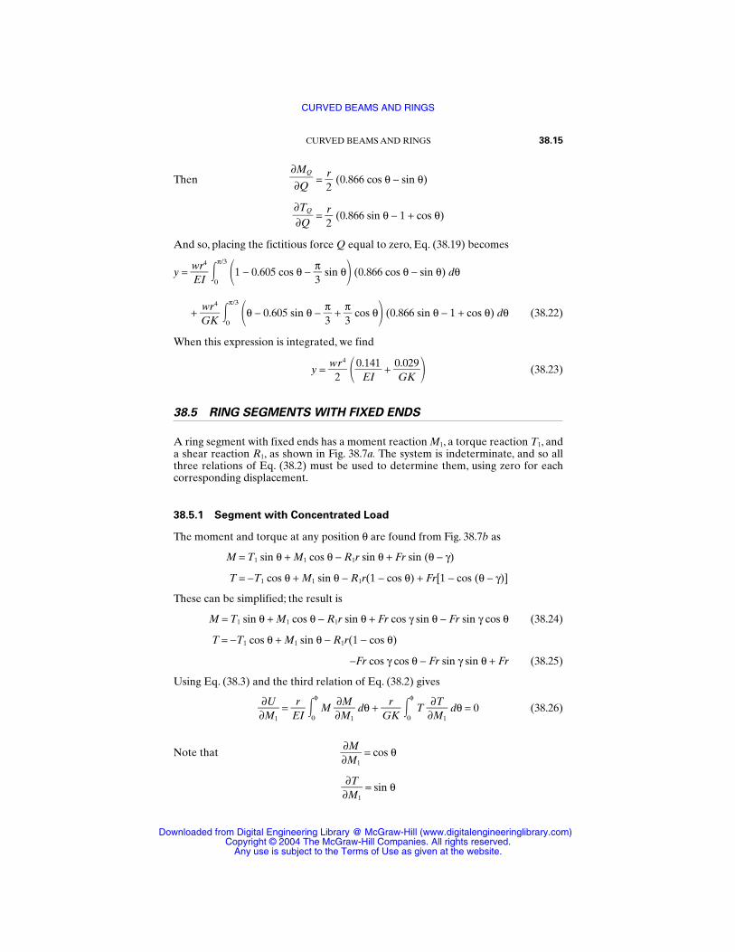
Then = 2r
(0.866 cos θ − sin θ)
= 2r
(0.866 sin θ − 1 + cos θ)
And so, placing the fictitious force Q equal to zero, Eq. (38.19) becomes
y = wE
rI
4
π/3
01 − 0.605 cos θ −
π3
sin θ (0.866 cos θ − sin θ) dθ
+ Gwr
K
4
π/3
0θ − 0.605 sin θ −
π3
+ π3
cos θ (0.866 sin θ − 1 + cos θ) dθ (38.22)
When this expression is integrated, we find
y = w
2r4
0.E14
I1
+ 0G.0
K29 (38.23)
38.5 RING SEGMENTS WITH FIXED ENDS
A ring segment with fixed ends has a moment reaction M1, a torque reaction T1, anda shear reaction R1, as shown in Fig. 38.7a. The system is indeterminate, and so allthree relations of Eq. (38.2) must be used to determine them, using zero for eachcorresponding displacement.
38.5.1 Segment with Concentrated Load
The moment and torque at any position θ are found from Fig. 38.7b as
M = T1 sin θ + M1 cos θ − R1r sin θ + Fr sin (θ − γ)
T = −T1 cos θ + M1 sin θ − R1r(1 − cos θ) + Fr[1 − cos (θ − γ)]
These can be simplified; the result is
M = T1 sin θ + M1 cos θ − R1r sin θ + Fr cos γ sin θ − Fr sin γ cos θ (38.24)
T = −T1 cos θ + M1 sin θ − R1r(1 − cos θ)
−Fr cos γ cos θ − Fr sin γ sin θ + Fr (38.25)
Using Eq. (38.3) and the third relation of Eq. (38.2) gives
∂∂MU
1 =
ErI φ
0M
∂∂MM
1 dθ +
GrK φ
0T
∂∂MT
1 dθ = 0 (38.26)
Note that ∂∂MM
1 = cos θ
∂∂MT
1 = sin θ
∂TQ∂Q
∂MQ∂Q
CURVED BEAMS AND RINGS 38.15
CURVED BEAMS AND RINGS
Downloaded from Digital Engineering Library @ McGraw-Hill (www.digitalengineeringlibrary.com)Copyright © 2004 The McGraw-Hill Companies. All rights reserved.
Any use is subject to the Terms of Use as given at the website.
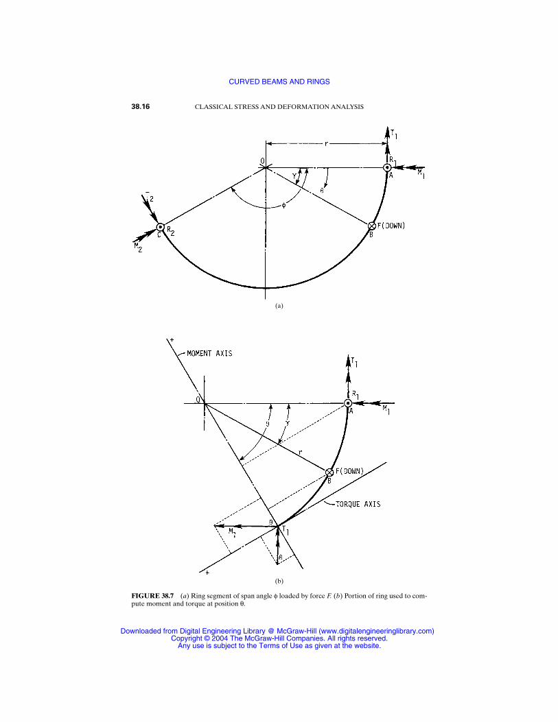
38.16 CLASSICAL STRESS AND DEFORMATION ANALYSIS
(a)
(b)
FIGURE 38.7 (a) Ring segment of span angle φ loaded by force F. (b) Portion of ring used to com-pute moment and torque at position θ.
CURVED BEAMS AND RINGS
Downloaded from Digital Engineering Library @ McGraw-Hill (www.digitalengineeringlibrary.com)Copyright © 2004 The McGraw-Hill Companies. All rights reserved.
Any use is subject to the Terms of Use as given at the website.

Now multiply Eq. (38.26) by EI and divide by r; then substitute. The result can bewritten in the form
φ
0(T1 sin θ + M1 cos θ − R1r sin θ) cos θ dθ
+ Fr φ
γ(cos γ sin θ − sin γ cos θ) cos θ dθ
+ GE
KI
φ
0[−T1 cos θ + M1 sin θ − R1r(1 − cos θ)] sin θ dθ
− Fr φ
γ(cos γ cos θ + sin γ sin θ − 1) sin θ dθ = 0 (38.27)
Similar equations can be written using the other two relations in Eq. (38.2). Whenthese three relations are integrated, the results can be expressed in the form
a11 a12 a13 T1/Fr b1a21 a22 a23 M1/Fr = b2 (38.28)
a31 a32 a33 R1/F b3
where
a11 = sin2 φ − GE
KI sin2 φ (38.29)
a21 = (φ − sin φ cos φ) + GE
KI (φ + sin φ cos φ) (38.30)
a31 = (φ − sin φ cos φ) + GE
KI (φ + sin φ cos φ − 2 sin φ) (38.31)
a12 = (φ + sin φ cos φ) + GE
KI (φ − sin φ cos φ) (38.32)
a22 = a11 (38.33)
a32 = sin2 φ + GE
KI [2(1 − cos φ) − sin2 φ] (38.34)
a13 = −a32 (38.35)
a23 = −a31 (38.36)
a33 = −(φ − sin φ cos φ) − GE
KI (3φ − 4 sin φ + sin φ cos φ) (38.37)
b1 = sin γ sin φ cos φ − cos γ sin2 φ + (φ − γ) sin γ + GE
KI [cos γ sin2 φ
− sin γ sin φ cos φ + (φ − γ)sin γ + 2 cos φ − 2 cos γ] (38.38)
CURVED BEAMS AND RINGS 38.17
CURVED BEAMS AND RINGS
Downloaded from Digital Engineering Library @ McGraw-Hill (www.digitalengineeringlibrary.com)Copyright © 2004 The McGraw-Hill Companies. All rights reserved.
Any use is subject to the Terms of Use as given at the website.
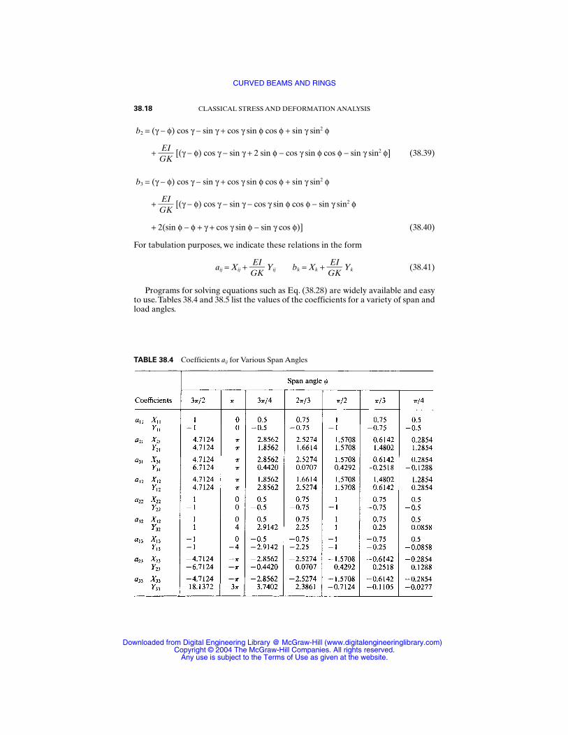
b2 = (γ − φ) cos γ − sin γ + cos γ sin φ cos φ + sin γ sin2 φ
+ GE
KI [(γ − φ) cos γ − sin γ + 2 sin φ − cos γ sin φ cos φ − sin γ sin2 φ] (38.39)
b3 = (γ − φ) cos γ − sin γ + cos γ sin φ cos φ + sin γ sin2 φ
+ GE
KI [(γ − φ) cos γ − sin γ − cos γ sin φ cos φ − sin γ sin2 φ
+ 2(sin φ − φ + γ + cos γ sin φ − sin γ cos φ)] (38.40)
For tabulation purposes, we indicate these relations in the form
aij = Xij + GE
KI Yij bk = Xk +
GE
KI Yk (38.41)
Programs for solving equations such as Eq. (38.28) are widely available and easyto use.Tables 38.4 and 38.5 list the values of the coefficients for a variety of span andload angles.
38.18 CLASSICAL STRESS AND DEFORMATION ANALYSIS
TABLE 38.4 Coefficients aij for Various Span Angles
CURVED BEAMS AND RINGS
Downloaded from Digital Engineering Library @ McGraw-Hill (www.digitalengineeringlibrary.com)Copyright © 2004 The McGraw-Hill Companies. All rights reserved.
Any use is subject to the Terms of Use as given at the website.
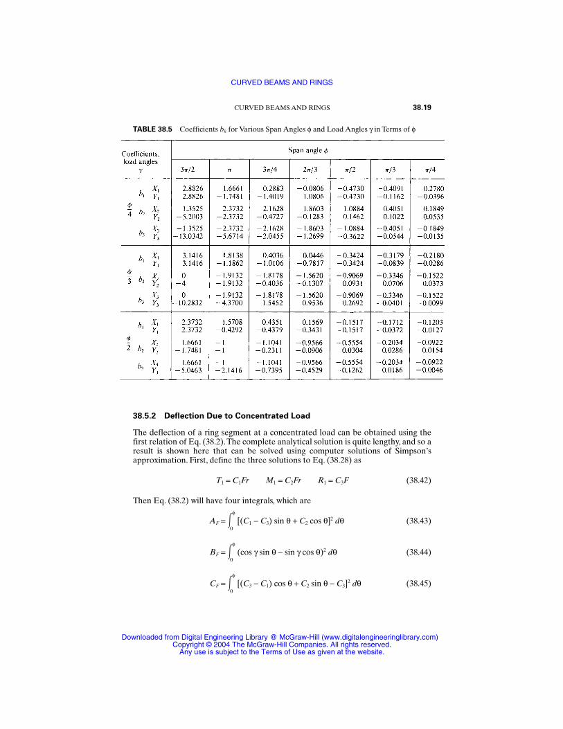
38.5.2 Deflection Due to Concentrated Load
The deflection of a ring segment at a concentrated load can be obtained using thefirst relation of Eq. (38.2).The complete analytical solution is quite lengthy, and so aresult is shown here that can be solved using computer solutions of Simpson’sapproximation. First, define the three solutions to Eq. (38.28) as
T1 = C1Fr M1 = C2Fr R1 = C3F (38.42)
Then Eq. (38.2) will have four integrals, which are
AF = φ
0[(C1 − C3) sin θ + C2 cos θ]2 dθ (38.43)
BF = φ
0(cos γ sin θ − sin γ cos θ)2 dθ (38.44)
CF = φ
0[(C3 − C1) cos θ + C2 sin θ − C3]2 dθ (38.45)
CURVED BEAMS AND RINGS 38.19
TABLE 38.5 Coefficients bk for Various Span Angles φ and Load Angles γ in Terms of φ
CURVED BEAMS AND RINGS
Downloaded from Digital Engineering Library @ McGraw-Hill (www.digitalengineeringlibrary.com)Copyright © 2004 The McGraw-Hill Companies. All rights reserved.
Any use is subject to the Terms of Use as given at the website.

DF = φ
0[1 − (cos γ cos θ + sin γ sin θ)]2 dθ (38.46)
The results of these four integrations should be substituted into
y = FE
rI
3
AF + BF + GE
KI (CF + DF) (38.47)
to obtain the deflection due to F and at the location of the force F.It is worth noting that the point of maximum deflection will never be far from the
middle of the ring, even though the force F may be exerted near one end.This meansthat Eq. (38.47) will not give the maximum deflection unless γ = φ/2.
38.5.3 Segment with Distributed Load
The resultant load acting at the centroid B′ in Fig. 38.8 is W = wrφ, and the radius r isgiven by Eq. (38.6), with φ substituted for θ. Thus the shear reaction at the fixed endA is R1 = wrφ/2. M1 and T1, at the fixed ends, can be determined using Castigliano’smethod.
We use Fig. 38.9 to write equations for moment and torque for any section, suchas the one at D. When Eq. (38.6) for r is used, the results are found to be
M = T1 sin θ + M1 cos θ − w
2r2φ sin θ + wr2(1 − cos θ) (38.48)
T = −T1 cos θ + M1 sin θ − w
2r2φ (1 − cos θ) + wr 2(θ − sin θ) (38.49)
38.20 CLASSICAL STRESS AND DEFORMATION ANALYSIS
FIGURE 38.8 Ring segment of span angle φ subjected to a uniformly dis-tributed load w per unit circumference acting downward. Point B′ is the centroidof the load. The ends are fixed to resist bending moment and torsional moment.
CURVED BEAMS AND RINGS
Downloaded from Digital Engineering Library @ McGraw-Hill (www.digitalengineeringlibrary.com)Copyright © 2004 The McGraw-Hill Companies. All rights reserved.
Any use is subject to the Terms of Use as given at the website.
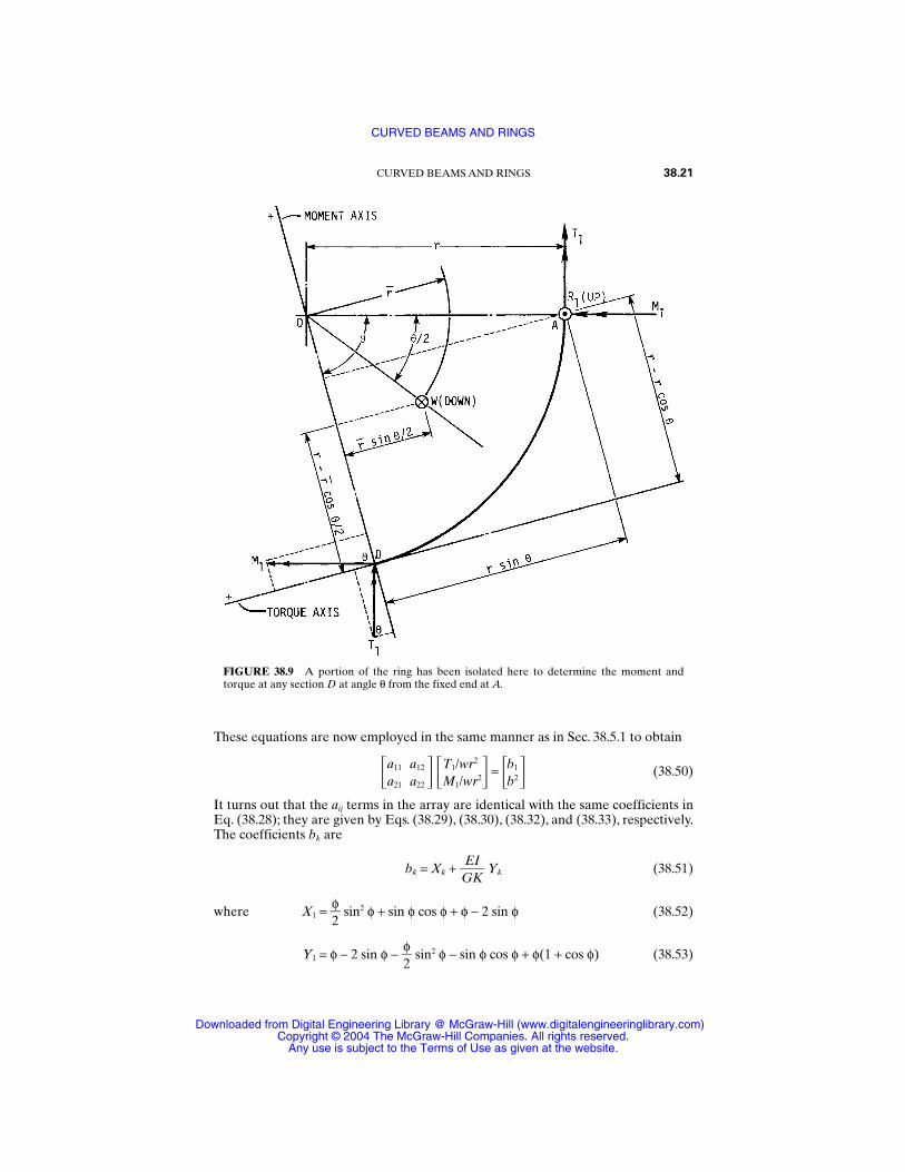
These equations are now employed in the same manner as in Sec. 38.5.1 to obtain
a11 a12 T1/wr2
= b1 (38.50)a21 a22 M1/wr2 b2
It turns out that the aij terms in the array are identical with the same coefficients inEq. (38.28); they are given by Eqs. (38.29), (38.30), (38.32), and (38.33), respectively.The coefficients bk are
bk = Xk + GE
KI Yk (38.51)
where X1 = φ2
sin2 φ + sin φ cos φ + φ − 2 sin φ (38.52)
Y1 = φ − 2 sin φ − φ2
sin2 φ − sin φ cos φ + φ(1 + cos φ) (38.53)
CURVED BEAMS AND RINGS 38.21
FIGURE 38.9 A portion of the ring has been isolated here to determine the moment andtorque at any section D at angle θ from the fixed end at A.
CURVED BEAMS AND RINGS
Downloaded from Digital Engineering Library @ McGraw-Hill (www.digitalengineeringlibrary.com)Copyright © 2004 The McGraw-Hill Companies. All rights reserved.
Any use is subject to the Terms of Use as given at the website.
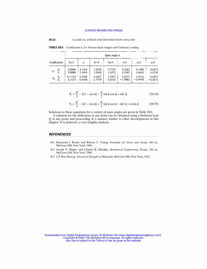
X2 = φ2
2
− 2(1 − cos φ) − φ2
sin φ cos φ + sin2 φ (38.54)
Y2 = φ2
2
− 2(1 − cos φ) + φ2
sin φ cos φ − sin2 φ + φ sin φ (38.55)
Solutions to these equations for a variety of span angles are given in Table 38.6.A solution for the deflection at any point can be obtained using a fictitious load
Q at any point and proceeding in a manner similar to other developments in thischapter. It is, however, a very lengthy analysis.
REFERENCES
38.1 Raymond J. Roark and Warren C. Young, Formulas for Stress and Strain, 6th ed.,McGraw-Hill, New York, 1984.
38.2 Joseph E. Shigley and Charles R. Mischke, Mechanical Engineering Design, 5th ed.,McGraw-Hill, New York, 1989.
38.3 J. P. Den Hartog, Advanced Strength of Materials, McGraw-Hill, New York, 1952.
38.22 CLASSICAL STRESS AND DEFORMATION ANALYSIS
TABLE 38.6 Coefficients bk for Various Span Angles and Uniform Loading
CURVED BEAMS AND RINGS
Downloaded from Digital Engineering Library @ McGraw-Hill (www.digitalengineeringlibrary.com)Copyright © 2004 The McGraw-Hill Companies. All rights reserved.
Any use is subject to the Terms of Use as given at the website.
CHAPTER 39PRESSURE CYLINDERS
Sachindranarayan Bhaduri, Ph.D.Associate Professor
Mechanical and Industrial Engineering DepartmentThe University of Texas at El Paso
El Paso, Texas
39.1 INTRODUCTION / 39.1
39.2 DESIGN PRINCIPLES OF PRESSURE CYLINDERS / 39.2
39.3 DESIGN LOADS / 39.3
39.4 CYLINDRICAL SHELLS—STRESS ANALYSIS / 39.4
39.5 THICK CYLINDRICAL SHELLS / 39.12
39.6 THERMAL STRESSES IN CYLINDRICAL SHELLS / 39.14
39.7 FABRICATION METHODS AND MATERIALS / 39.17
39.8 DESIGN OF PRESSURE CYLINDERS / 39.18
REFERENCES / 39.21
39.1 INTRODUCTION
The pressure vessels commonly used in industrial applications consist basically of afew closed shells of simple shape: spherical or cylindrical with hemispherical, coni-cal, ellipsoidal, or flat ends. The shell components are joined together mostly bywelding and riveting; sometimes they are bolted together using flanges.
Generally, the shell elements are axisymmetrical surfaces of revolution formedby rotation of a straight line or a plane curve known as a meridian or a generatorabout an axis of rotation. The plane containing the axis of rotation is called themeridional plane. The geometry of such simple shells is specified by the form of themidwall surface, usually two radii of curvature and the wall thickness at every point.The majority of pressure vessels are cylindrical.
In practice, the shell is considered thin if the wall thickness t is small in compari-son with the circumferential radius of curvature Rθ and the longitudinal radius ofcurvature R. If the ratio Rθ/t > 10, the shell is considered to be thin shell.This impliesthat the stresses developed in the shell wall by external loads can be considered tobe uniformly distributed over the wall thickness. Many shells used in pressure-vesselconstruction are relatively thin (10 < Rθ/t < 500), with the associated uniform distri-bution of stresses throughout the cylinder wall. Bending stresses in the walls of suchmembrane shells due to concentrated external loads are of higher intensity near thearea of application of the load. The attenuation distance from the load where thestresses die out is short. The radial deformation of a shell subjected to internal pres-sure is assumed smaller than one-half the shell thickness. The shell thickness isdesigned to keep the maximum stresses below the yield strength of the material.
39.1
Source: STANDARD HANDBOOK OF MACHINE DESIGN
Downloaded from Digital Engineering Library @ McGraw-Hill (www.digitalengineeringlibrary.com)Copyright © 2004 The McGraw-Hill Companies. All rights reserved.
Any use is subject to the Terms of Use as given at the website.

39.2 DESIGN PRINCIPLES OF PRESSURE CYLINDERS
In the design of a pressure vessel as a unit, a number of criteria should be consid-ered. These are (1) selection of the material for construction of the vessel based ona working knowledge of the properties of the material, (2) determination of themagnitude of the induced stress in conformity with the requirements of standardcodes, and (3) determination of the elastic stability. To simplify the design and keepthe cost of fabrication low, the components of a vessel should be made in the form ofsimple geometric shapes, such as spherical, cylindrical, or conical. A spherical geom-etry provides minimum surface area per unit volume and requires minimum wallthickness for a given pressure. From the point of view of material savings and uni-form distribution of induced stresses in the shell wall, a spherical shape is favorable.However, the fabrication of spherical vessels is more complicated and expensivethan that of cylindrical ones. Spherical vessels are used commonly for storage of gasand liquids. For large-volume, low-pressure storage, spherical vessels are economi-cal. But for higher-pressure storage, cylindrical vessels are more economical.
The most common types of vessels can be classified according to their
1. Functions: Storage vessels, reactors, boilers, mixers, and heat exchangers2. Structural materials: Steel, cast iron, copper, plastics, etc.3. Method of fabrication: Welded, cast, brazed, flanged, etc.4. Geometry: Cylindrical, spherical, conical, combined5. Scheme of loading: Working under internal or external pressure6. Wall temperatures: Heated, unheated7. Corrosion action: Moderate or high corrosion effects8. Orientation in space: Vertical, horizontal, sloped9. Method of assembly: Detachable, nondetachable
10. Wall thickness: Thin-walled (do/di < 1.5); thick-walled (do/di ≥ 1.5)
Most vessels are designed as cylindrical shells fabricated of rolled sheet metal oras cylindrical shells that are cast. From the point of view of simplified structuraldesign, the stressed state of the material of a thin-wall shell is considered biaxial.This is permissible because the magnitude of the radial stress in such a vessel wall isvery small. The stressed state of the shell wall is generally the sum of the two basiccomponents: (1) stressed state due to uniformly distributed forces on the surface asa result of fluid pressure, and (2) stressed state due to the action of the forces andmoments distributed around the contour.
The stressed condition due to uniform pressure of fluid on the surface of the shellcan be determined either by the membrane or moment theory. The membrane the-ory yields accurate enough results for most engineering applications and is widelyused for structural designs. The moment theory is not usually applied for the deter-mination of stresses due to uniformly distributed fluid forces on a surface.The equa-tions resulting from the application of the moment theory are complex and thedesign process is quite involved.
End forces and moments are calculated in sections where a sudden change inload, wall thickness, or the properties of the shell material occurs. The stressed stateinduced by the applied end forces and moments are determined by application ofthe moment theory [39.1]. The induced stress and deformations due to end effects
39.2 CLASSICAL STRESS AND DEFORMATION ANALYSIS
PRESSURE CYLINDERS
Downloaded from Digital Engineering Library @ McGraw-Hill (www.digitalengineeringlibrary.com)Copyright © 2004 The McGraw-Hill Companies. All rights reserved.
Any use is subject to the Terms of Use as given at the website.
influence mostly the zones where the end forces and moments are applied. In gen-eral, end stresses should be carefully evaluated, and design measures must be takento keep them within the safe limit. High values of end stresses are to be avoided,especially for brittle materials and vessels operating under high alternating loads.
The structural reliability of the equipment parts is determined by two differentapproaches. The theory of elasticity requires that the strength be determined by theultimate stress which the part can withstand without rupture, whereas the theory ofplasticity suggests that the strength be determined by the ultimate load the part canwithstand without residual deformation. The elastic theory is based on the assump-tion that the material of the component parts of the vessel is in an elastic state every-where and nowhere does the state of stress exceed the yield point.
The parts of a pressure vessel are not generally bonded uniformly. When thestructural design is based on the ultimate stress occurring at the most loaded regionof the construction, the required material consumption could be excessive. In designworks using the membrane theory, only average stresses are assumed, and no effortsare made to include the local stresses of significant magnitude. However, thedesigner should consider the probable adverse effects of very high local stress inten-sities and modify the design accordingly.
In heavily loaded parts of pressure vessels made of plastic materials, partial tran-sition to the elastic-plastic state occurs. The plastic design method permits a realisticevaluation of the maximum load this vessel can withstand without failure.
39.3 DESIGN LOADS
The principal loads (i.e., forces) applied in actual operations to a vessel or its struc-tural attachments to be considered in the design of such a vessel are
1. Design pressure (internal or external or both)2. Dead loads3. Wind loads4. Thermal loads5. Piping load6. Impact load7. Cyclic loads
Several loading combinations are often possible. The designer should considerthem carefully for a particular situation and select the most probable combinationof simultaneous loads for an economical and reliable design. Failure of a pressurevessel may be due to improper selection of materials, defects in materials due toinadequate quality control, incorrect design conditions, computational errors indesign, improper or faulty fabrication procedures, or inadequate inspection andshop testing.
Design pressure is the pressure used to determine the minimum thickness of eachof the vessel components. It is the difference between the internal and external pres-sures.A suitable margin above the operating pressure (usually 10 percent of operat-ing pressure and a minimum of 10 psi) plus a static head of operating liquid must beincluded. The minimum design pressure for a “code” nonvacuum vessel is 15 psi.Vessels with negative gauge operating pressures are designed for full vacuum. In
PRESSURE CYLINDERS 39.3
PRESSURE CYLINDERS
Downloaded from Digital Engineering Library @ McGraw-Hill (www.digitalengineeringlibrary.com)Copyright © 2004 The McGraw-Hill Companies. All rights reserved.
Any use is subject to the Terms of Use as given at the website.
determining the design load, the designer must consult the ASME Boiler and Pres-sure Vessel Code, Sec. VIII, Pressure Vessels, Division I. The maximum operatingpressure is, according to code definition, the maximum gauge pressure permissible atthe top of the completed vessel in its operating condition at the designated temper-ature. It is based on the nominal thickness, exclusive of the corrosion allowance, andthe thickness required for loads other than fluid pressure.
The required thickness is the minimum thickness of the vessel wall, computed bycode formula. The design thickness is the minimum required thickness plus anallowance for corrosion. The nominal thickness is the design thickness of the com-mercially available material actually used in making the vessel.
The vessel shell must be designed to withstand the combined effect of the pres-sure and temperature under the anticipated operating conditions. One has to use thepressure-vessel code and standard engineering analysis whenever applicable todetermine the nominal stress at any part of the vessel.The stresses cannot in generalexceed the allowable stress obtained by the code guidelines.
Design temperature is really more a design environmental condition than a load.Thermal loads originate from temperature changes combined with body restraintsor existing temperature gradients. Reduction in structural strength due to risingtemperature, increase in brittleness with rapidly falling temperature, and the associ-ated changes in the vessel dimensions should be taken into careful consideration forthe design. The code design temperature must not be less than the mean vessel-walltemperature under operating conditions. It can be determined by the standard heat-transfer methods. Generally, the standard vessel design temperature is equal to themaximum operating temperature of the fluid in the vessel plus 50°F for safety con-siderations. For low-temperature operation, the minimum fluid temperature is usedfor the design temperature. The designer should consult the ASME Boiler and Pres-sure Vessel Codes and the excellent books by Bednar [39.2] and Chuse [39.3].
Dead loads are the forces due to the weight of the vessel and the parts perma-nently connected with the vessel.The piping loads acting on the vessel must be eval-uated carefully. They consist of the weight of the pipe sections supported by thenozzles into the vessel shell, as well as operating forces due to thermal expansion ofthe pipes.
If the pressure vessel is exposed to the environment, the dynamic pressure forcesdue to the turbulent flow of air and associated gustiness must be evaluated for struc-tural stability of the vessel support system. Determination of wind load is outlined inthe SEI/ASCE 7-02 standard, and the designer must follow the guidelines to deter-mine the effective dynamic load due to wind speed past the vessel and support-structure system. The same code provides guidelines for evaluation of seismic loadson flexible tall vessels.
In actual design situations, many combinations of loads are possible. Conse-quently, the designer should use discretion to determine the important ones andselect only certain sets of design loads which can most probably occur simultane-ously.
39.4 CYLINDRICAL SHELLS—STRESS ANALYSIS
Cylindrical shells are widely used in the manufacture of pressure vessels. They canbe easily fabricated and have great structural strength. Depending on their func-tion, they may be vertical or horizontal. Vertical pressure vessels are often pre-ferred, especially for a thin-walled vessel operating under low internal pressure.
39.4 CLASSICAL STRESS AND DEFORMATION ANALYSIS
PRESSURE CYLINDERS
Downloaded from Digital Engineering Library @ McGraw-Hill (www.digitalengineeringlibrary.com)Copyright © 2004 The McGraw-Hill Companies. All rights reserved.
Any use is subject to the Terms of Use as given at the website.
The design of a vertical cylindrical vessel becomes simple because the additionalbending stresses due to weight of the vessel itself and of the fluid can be elimi-nated.
Cylindrical shells of malleable materials, such as steels, nonferrous metals, andtheir alloys, operating under internal pressures up to 10 MPa are fabricated mostlyof rolled and welded sheets of corrosion-resistant material (see Ref. [39.1]). Theminimum thickness of a shell rolled from low-carbon sheet metal and welded is 4.0mm.The minimum thickness for an austenitic steel shell is 3.4 mm; for copper shells,2.5 to 30 mm; and for cast shells, 20 to 25 mm.
39.4.1 Cylindrical Storage Vessel
Before the actual design calculation of a vertical cylindrical vessel is done, the rela-tionship between the optimum height and the diameter should be determined. Thevolume of the sheet metal needed to make a vertical cylindrical storage tank (Fig.39.1) is determined by the following formula:
Vs = πdoHt1 + (tk + ta)
= πdoHt1 + t2 (39.1)
Vessel capacity is
V = H (39.2)
The inside diameter of the vessel is
di = (39.3)
Since thickness t1 is very small in comparison with do and di, we may consider di ≈ do.Substitution of Eq. (39.3) into Eq. (39.1) gives
Vs = 2t1πVH + (39.4)
The minimum volume of sheet metal is obtained by differentiating Eq. (39.4) withrespect to H and equating the derivative to zero. Thus
= t1πV/H − = 0 (39.5)
The optimum height and the optimum diameter of the tank are given by
Hopt = 21/3(39.6)
and dopt = 2 1/3(39.7)
Vt1πt2
t2t1
Vπ
Vt2H2
dVsdH
Vt2H
4VπH
πdi2
4
πd2o
4
πd2o
4
PRESSURE CYLINDERS 39.5
PRESSURE CYLINDERS
Downloaded from Digital Engineering Library @ McGraw-Hill (www.digitalengineeringlibrary.com)Copyright © 2004 The McGraw-Hill Companies. All rights reserved.
Any use is subject to the Terms of Use as given at the website.
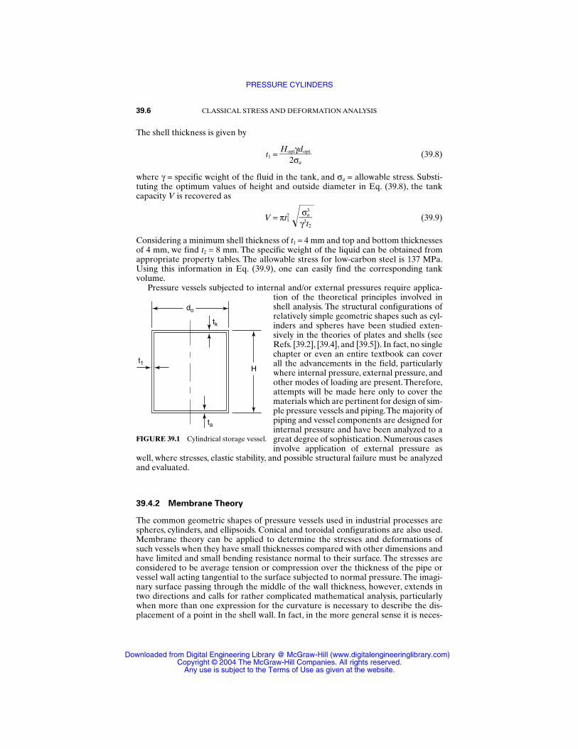
The shell thickness is given by
t1 = (39.8)
where γ = specific weight of the fluid in the tank, and σa = allowable stress. Substi-tuting the optimum values of height and outside diameter in Eq. (39.8), the tankcapacity V is recovered as
V = πt21 (39.9)
Considering a minimum shell thickness of t1 = 4 mm and top and bottom thicknessesof 4 mm, we find t2 = 8 mm. The specific weight of the liquid can be obtained fromappropriate property tables. The allowable stress for low-carbon steel is 137 MPa.Using this information in Eq. (39.9), one can easily find the corresponding tank volume.
Pressure vessels subjected to internal and/or external pressures require applica-tion of the theoretical principles involved inshell analysis. The structural configurations ofrelatively simple geometric shapes such as cyl-inders and spheres have been studied exten-sively in the theories of plates and shells (seeRefs. [39.2], [39.4], and [39.5]). In fact, no singlechapter or even an entire textbook can coverall the advancements in the field, particularlywhere internal pressure, external pressure, andother modes of loading are present. Therefore,attempts will be made here only to cover thematerials which are pertinent for design of sim-ple pressure vessels and piping.The majority ofpiping and vessel components are designed forinternal pressure and have been analyzed to agreat degree of sophistication. Numerous casesinvolve application of external pressure as
well, where stresses, elastic stability, and possible structural failure must be analyzedand evaluated.
39.4.2 Membrane Theory
The common geometric shapes of pressure vessels used in industrial processes arespheres, cylinders, and ellipsoids. Conical and toroidal configurations are also used.Membrane theory can be applied to determine the stresses and deformations ofsuch vessels when they have small thicknesses compared with other dimensions andhave limited and small bending resistance normal to their surface. The stresses areconsidered to be average tension or compression over the thickness of the pipe orvessel wall acting tangential to the surface subjected to normal pressure. The imagi-nary surface passing through the middle of the wall thickness, however, extends intwo directions and calls for rather complicated mathematical analysis, particularlywhen more than one expression for the curvature is necessary to describe the dis-placement of a point in the shell wall. In fact, in the more general sense it is neces-
σ3a
γ3t2
Hoptγdopt2σa
39.6 CLASSICAL STRESS AND DEFORMATION ANALYSIS
do
tk
t1H
ta
FIGURE 39.1 Cylindrical storage vessel.
PRESSURE CYLINDERS
Downloaded from Digital Engineering Library @ McGraw-Hill (www.digitalengineeringlibrary.com)Copyright © 2004 The McGraw-Hill Companies. All rights reserved.
Any use is subject to the Terms of Use as given at the website.
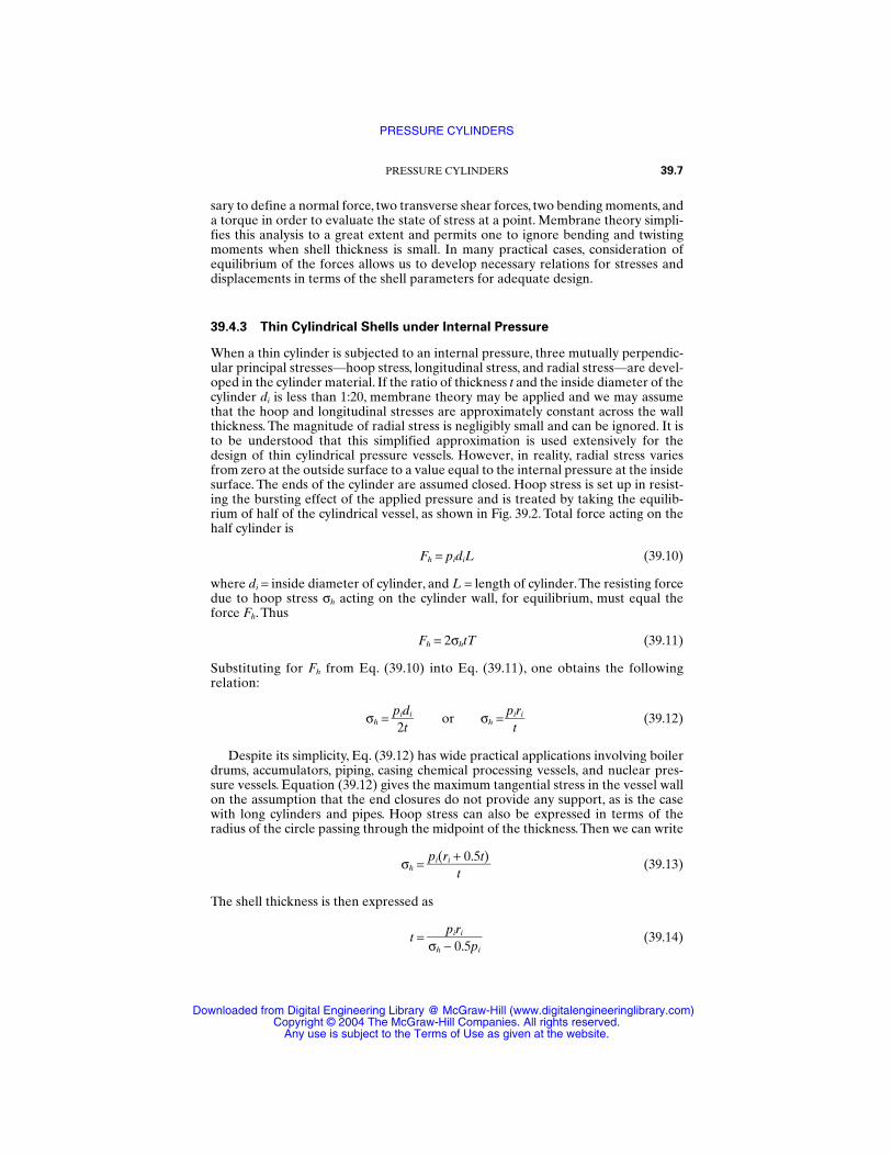
sary to define a normal force, two transverse shear forces, two bending moments, anda torque in order to evaluate the state of stress at a point. Membrane theory simpli-fies this analysis to a great extent and permits one to ignore bending and twistingmoments when shell thickness is small. In many practical cases, consideration ofequilibrium of the forces allows us to develop necessary relations for stresses anddisplacements in terms of the shell parameters for adequate design.
39.4.3 Thin Cylindrical Shells under Internal Pressure
When a thin cylinder is subjected to an internal pressure, three mutually perpendic-ular principal stresses—hoop stress, longitudinal stress, and radial stress—are devel-oped in the cylinder material. If the ratio of thickness t and the inside diameter of thecylinder di is less than 1:20, membrane theory may be applied and we may assumethat the hoop and longitudinal stresses are approximately constant across the wallthickness. The magnitude of radial stress is negligibly small and can be ignored. It isto be understood that this simplified approximation is used extensively for thedesign of thin cylindrical pressure vessels. However, in reality, radial stress variesfrom zero at the outside surface to a value equal to the internal pressure at the insidesurface. The ends of the cylinder are assumed closed. Hoop stress is set up in resist-ing the bursting effect of the applied pressure and is treated by taking the equilib-rium of half of the cylindrical vessel, as shown in Fig. 39.2. Total force acting on thehalf cylinder is
Fh = pidiL (39.10)
where di = inside diameter of cylinder, and L = length of cylinder.The resisting forcedue to hoop stress σh acting on the cylinder wall, for equilibrium, must equal theforce Fh. Thus
Fh = 2σhtT (39.11)
Substituting for Fh from Eq. (39.10) into Eq. (39.11), one obtains the followingrelation:
σh = or σh = (39.12)
Despite its simplicity, Eq. (39.12) has wide practical applications involving boilerdrums, accumulators, piping, casing chemical processing vessels, and nuclear pres-sure vessels. Equation (39.12) gives the maximum tangential stress in the vessel wallon the assumption that the end closures do not provide any support, as is the casewith long cylinders and pipes. Hoop stress can also be expressed in terms of theradius of the circle passing through the midpoint of the thickness.Then we can write
σh = (39.13)
The shell thickness is then expressed as
t = (39.14)piri
σh − 0.5pi
pi(ri + 0.5t)
t
pirit
pidi2t
PRESSURE CYLINDERS 39.7
PRESSURE CYLINDERS
Downloaded from Digital Engineering Library @ McGraw-Hill (www.digitalengineeringlibrary.com)Copyright © 2004 The McGraw-Hill Companies. All rights reserved.
Any use is subject to the Terms of Use as given at the website.
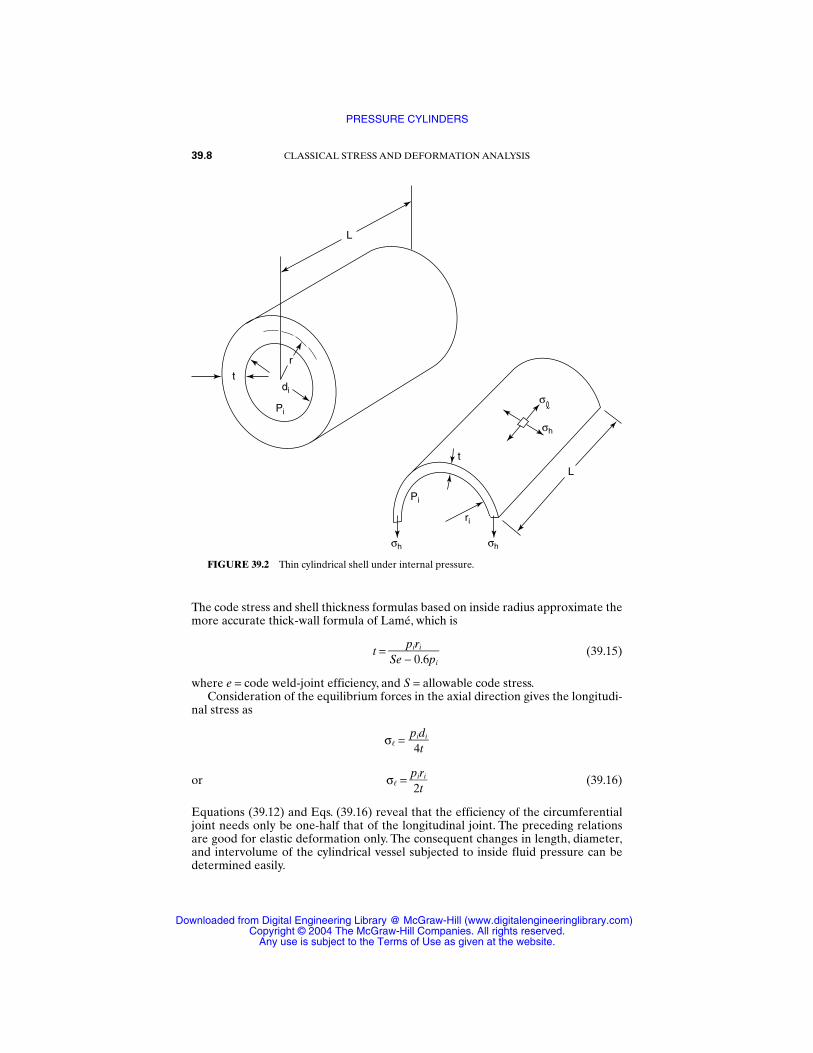
The code stress and shell thickness formulas based on inside radius approximate themore accurate thick-wall formula of Lamé, which is
t = (39.15)
where e = code weld-joint efficiency, and S = allowable code stress.Consideration of the equilibrium forces in the axial direction gives the longitudi-
nal stress as
σ =
or σ = (39.16)
Equations (39.12) and Eqs. (39.16) reveal that the efficiency of the circumferentialjoint needs only be one-half that of the longitudinal joint. The preceding relationsare good for elastic deformation only. The consequent changes in length, diameter,and intervolume of the cylindrical vessel subjected to inside fluid pressure can bedetermined easily.
piri2t
pidi4t
piriSe − 0.6pi
39.8 CLASSICAL STRESS AND DEFORMATION ANALYSIS
di
σh
σhσh
σPi
Pi
r
L
t
tL
ri
FIGURE 39.2 Thin cylindrical shell under internal pressure.
PRESSURE CYLINDERS
Downloaded from Digital Engineering Library @ McGraw-Hill (www.digitalengineeringlibrary.com)Copyright © 2004 The McGraw-Hill Companies. All rights reserved.
Any use is subject to the Terms of Use as given at the website.
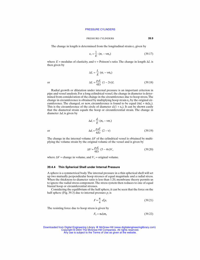
The change in length is determined from the longitudinal strain ε given by
ε = (σ − νσh) (39.17)
where E = modulus of elasticity, and ν = Poisson’s ratio. The change in length ∆L isthen given by
∆L = (σ − νσh)
or ∆L = (1 − 2ν)L (39.18)
Radial growth or dilatation under internal pressure is an important criterion inpipe and vessel analysis. For a long cylindrical vessel, the change in diameter is deter-mined from consideration of the change in the circumference due to hoop stress.Thechange in circumference is obtained by multiplying hoop strain εh by the original cir-cumference. The changed, or new, circumference is found to be equal (πdi + πdiεh).This is the circumference of the circle of diameter di(1 + εh). It can be shown easilythat the diametral strain equals the hoop or circumferential strain. The change indiameter ∆di is given by
∆di = (σh − νσ)
or ∆di = (2 − ν) (39.19)
The change in the internal volume ∆V of the cylindrical vessel is obtained by multi-plying the volume strain by the original volume of the vessel and is given by
∆V = (5 − 4ν)Vo (39.20)
where ∆V = change in volume, and Vo = original volume.
39.4.4 Thin Spherical Shell under Internal Pressure
A sphere is a symmetrical body.The internal pressure in a thin spherical shell will setup two mutually perpendicular hoop stresses of equal magnitude and a radial stress.When the thickness-to-diameter ratio is less than 1:20, membrane theory permits usto ignore the radial stress component.The stress system then reduces to one of equalbiaxial hoop or circumferential stresses.
Considering the equilibrium of the half sphere, it can be seen that the force on thehalf sphere (Fig. 39.3) due to internal pressure pi is
F = di2pi (39.21)
The resisting force due to hoop stress is given by
Fh = πditσh (39.22)
π4
pidi4Et
pidi2
4Et
diE
pidi4Et
LE
1E
PRESSURE CYLINDERS 39.9
PRESSURE CYLINDERS
Downloaded from Digital Engineering Library @ McGraw-Hill (www.digitalengineeringlibrary.com)Copyright © 2004 The McGraw-Hill Companies. All rights reserved.
Any use is subject to the Terms of Use as given at the website.
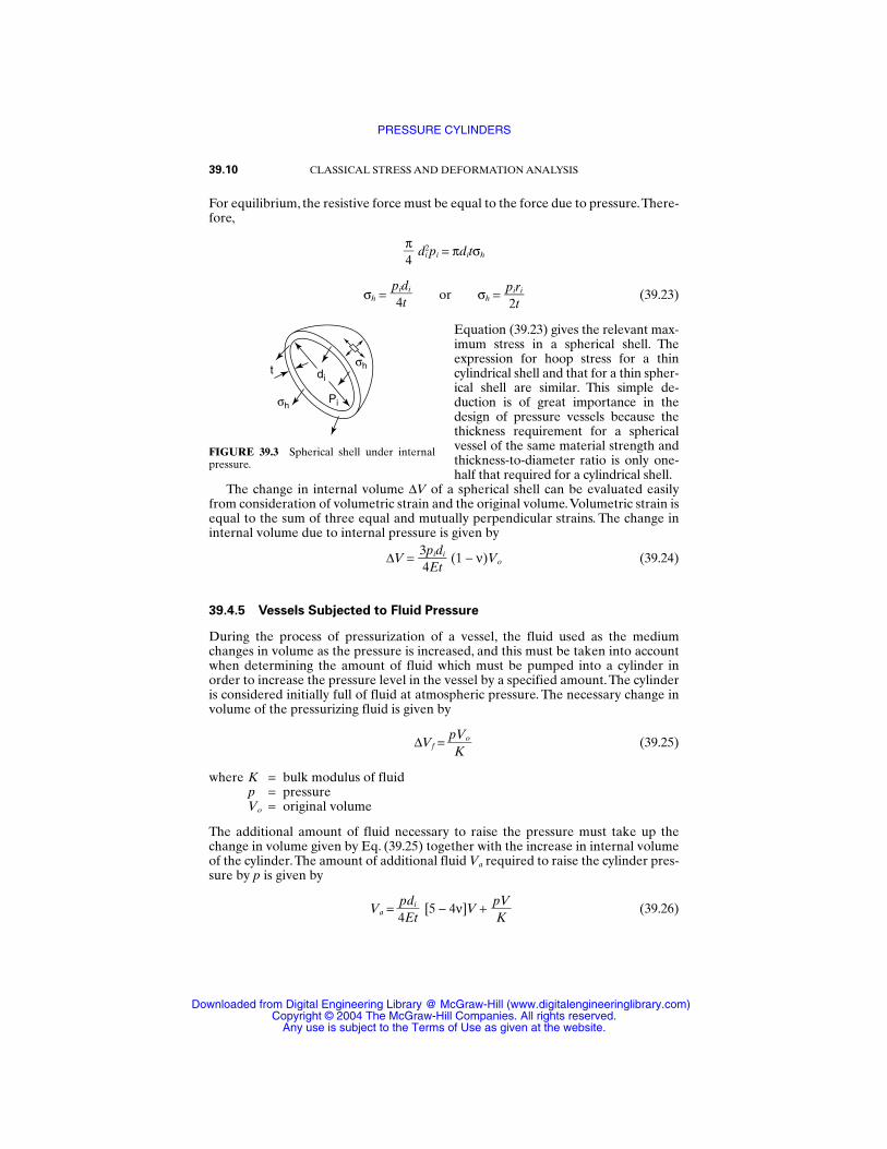
For equilibrium, the resistive force must be equal to the force due to pressure.There-fore,
di2pi = πditσh
σh = or σh = (39.23)
Equation (39.23) gives the relevant max-imum stress in a spherical shell. Theexpression for hoop stress for a thincylindrical shell and that for a thin spher-ical shell are similar. This simple de-duction is of great importance in thedesign of pressure vessels because thethickness requirement for a sphericalvessel of the same material strength andthickness-to-diameter ratio is only one-half that required for a cylindrical shell.
The change in internal volume ∆V of a spherical shell can be evaluated easilyfrom consideration of volumetric strain and the original volume.Volumetric strain isequal to the sum of three equal and mutually perpendicular strains. The change ininternal volume due to internal pressure is given by
∆V = (1 − ν)Vo (39.24)
39.4.5 Vessels Subjected to Fluid Pressure
During the process of pressurization of a vessel, the fluid used as the mediumchanges in volume as the pressure is increased, and this must be taken into accountwhen determining the amount of fluid which must be pumped into a cylinder inorder to increase the pressure level in the vessel by a specified amount.The cylinderis considered initially full of fluid at atmospheric pressure. The necessary change involume of the pressurizing fluid is given by
∆Vf = (39.25)
where K = bulk modulus of fluidp = pressureVo = original volume
The additional amount of fluid necessary to raise the pressure must take up thechange in volume given by Eq. (39.25) together with the increase in internal volumeof the cylinder.The amount of additional fluid Va required to raise the cylinder pres-sure by p is given by
Va = [5 − 4ν]V + (39.26)pVK
pdi4Et
pVoK
3pidi4Et
piri2t
pidi4t
π4
39.10 CLASSICAL STRESS AND DEFORMATION ANALYSIS
di
σh
σhPi
t
FIGURE 39.3 Spherical shell under internalpressure.
PRESSURE CYLINDERS
Downloaded from Digital Engineering Library @ McGraw-Hill (www.digitalengineeringlibrary.com)Copyright © 2004 The McGraw-Hill Companies. All rights reserved.
Any use is subject to the Terms of Use as given at the website.

It can be shown by similar analysis that the additional volume of fluid Va required topressurize a spherical vessel is given by
Va = (1 − ν)V + (39.27)
39.4.6 Cylindrical Vessel with Hemispherical Ends
One of the most commonly used configurations of pressure vessels is a cylindricalvessel with hemispherical ends, as shown in Fig. 39.4. The wall thickness of the cylin-drical and hemispherical parts may be different. This is often necessary because thehoop stress in the cylinder is twice that in a sphere of the same inside diameter andwall thickness. The internal diameters of both parts are generally considered equal.In order that there should be no distortion or mismatch of hoop stress at the junc-tion, the hoop stresses for the cylindrical part and the hemispherical part must beequal at the end junctions. Therefore,
[2 − ν] = [1 − ν] (39.28)
where tc = thickness of the cylinder, and ts = thickness of the hemisphere. Simplifica-tion of Eq. (39.28) gives
= (39.29)
39.4.7 Effects of Joints and End Plates in Vessel Fabrication
The preceding sections have assumed homogeneous materials and uniform materialproperties of the components. The effects of the end plates and joints will be thereduction of strength of the components due to characteristic fabrication tech-niques, such as riveted joints, welding, etc. To some extent, this reduction is takeninto account by using a parameter, joint efficiency, in the equation of the stresses. Fora thin cylindrical vessel as depicted in Fig. 39.5 the actual hoop and longitudinalstresses are given by the following equations:
σh = (39.30)pdi2tηl
(1 − v)(2 − v)
tstc
pdi4Ets
pdi4Etc
pVK
3pdi4Et
PRESSURE CYLINDERS 39.11
ts
tc
diP
FIGURE 39.4 Thin cylindrical shell with hemispherical ends.
PRESSURE CYLINDERS
Downloaded from Digital Engineering Library @ McGraw-Hill (www.digitalengineeringlibrary.com)Copyright © 2004 The McGraw-Hill Companies. All rights reserved.
Any use is subject to the Terms of Use as given at the website.
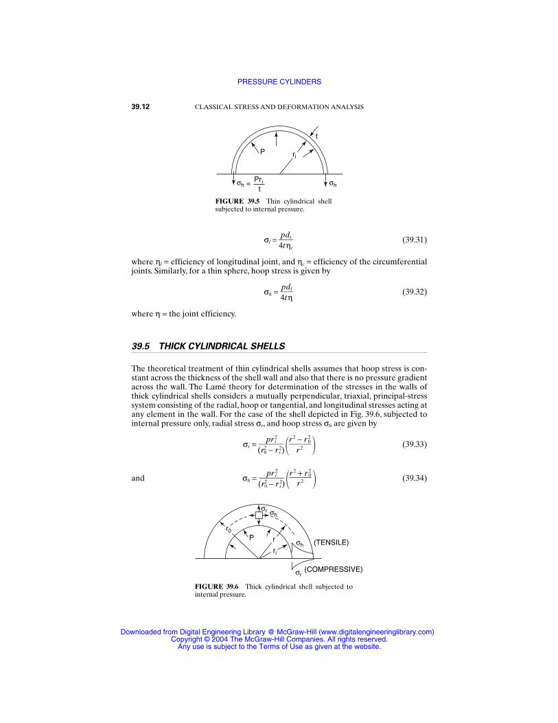
σl = (39.31)
where ηl = efficiency of longitudinal joint, and ηc = efficiency of the circumferentialjoints. Similarly, for a thin sphere, hoop stress is given by
σh = (39.32)
where η = the joint efficiency.
39.5 THICK CYLINDRICAL SHELLS
The theoretical treatment of thin cylindrical shells assumes that hoop stress is con-stant across the thickness of the shell wall and also that there is no pressure gradientacross the wall. The Lamé theory for determination of the stresses in the walls ofthick cylindrical shells considers a mutually perpendicular, triaxial, principal-stresssystem consisting of the radial, hoop or tangential, and longitudinal stresses acting atany element in the wall. For the case of the shell depicted in Fig. 39.6, subjected tointernal pressure only, radial stress σr, and hoop stress σh are given by
σr = (39.33)
and σh = (39.34)r 2 + r 2
0r 2
pr 2i
(r20 − r 2
i)
r 2 − r 20
r 2
pr 2i
(r20 − r 2
i)
pdl4tη
pdt4tηc
39.12 CLASSICAL STRESS AND DEFORMATION ANALYSIS
t
t
ri
σhσh
P
Pri=
FIGURE 39.5 Thin cylindrical shellsubjected to internal pressure.
r
ri
σh (TENSILE)
(COMPRESSIVE)
r0
σr
σr
σh
P
FIGURE 39.6 Thick cylindrical shell subjected tointernal pressure.
PRESSURE CYLINDERS
Downloaded from Digital Engineering Library @ McGraw-Hill (www.digitalengineeringlibrary.com)Copyright © 2004 The McGraw-Hill Companies. All rights reserved.
Any use is subject to the Terms of Use as given at the website.
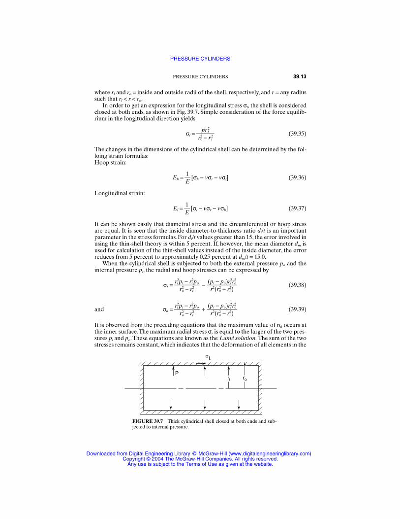
where rl and ro = inside and outside radii of the shell, respectively, and r = any radiussuch that rl < r < ro.
In order to get an expression for the longitudinal stress σt, the shell is consideredclosed at both ends, as shown in Fig. 39.7. Simple consideration of the force equilib-rium in the longitudinal direction yields
σl = (39.35)
The changes in the dimensions of the cylindrical shell can be determined by the fol-loing strain formulas:Hoop strain:
Eh = [σh − vσr − vσl] (39.36)
Longitudinal strain:
El = [σl − vσr − vσh] (39.37)
It can be shown easily that diametral stress and the circumferential or hoop stressare equal. It is seen that the inside diameter-to-thickness ratio di/t is an importantparameter in the stress formulas. For di/t values greater than 15, the error involved inusing the thin-shell theory is within 5 percent. If, however, the mean diameter dm isused for calculation of the thin-shell values instead of the inside diameter, the errorreduces from 5 percent to approximately 0.25 percent at dm/t = 15.0.
When the cylindrical shell is subjected to both the external pressure po and theinternal pressure pi, the radial and hoop stresses can be expressed by
σr = − (39.38)
and σh = + (39.39)
It is observed from the preceding equations that the maximum value of σh occurs atthe inner surface.The maximum radial stress σr is equal to the larger of the two pres-sures pi and po.These equations are known as the Lamé solution. The sum of the twostresses remains constant, which indicates that the deformation of all elements in the
(pi − po)ri2r2
or2(r2
o − ri2)
ri2pi − r2
opor2
o − ri2
(pi − po)ri2r2
or2(r2
o − ri2)
ri2pi − r2
opor2
o − ri2
1E
1E
pr 2i
r20 − r 2
i
PRESSURE CYLINDERS 39.13
Pri ro
σ
FIGURE 39.7 Thick cylindrical shell closed at both ends and sub-jected to internal pressure.
PRESSURE CYLINDERS
Downloaded from Digital Engineering Library @ McGraw-Hill (www.digitalengineeringlibrary.com)Copyright © 2004 The McGraw-Hill Companies. All rights reserved.
Any use is subject to the Terms of Use as given at the website.
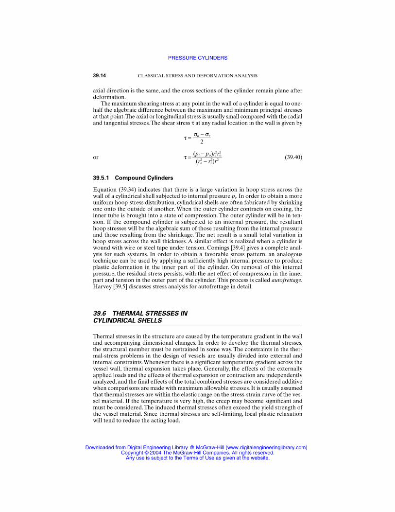
axial direction is the same, and the cross sections of the cylinder remain plane afterdeformation.
The maximum shearing stress at any point in the wall of a cylinder is equal to one-half the algebraic difference between the maximum and minimum principal stressesat that point.The axial or longitudinal stress is usually small compared with the radialand tangential stresses.The shear stress τ at any radial location in the wall is given by
τ =
or τ = (39.40)
39.5.1 Compound Cylinders
Equation (39.34) indicates that there is a large variation in hoop stress across thewall of a cylindrical shell subjected to internal pressure pi. In order to obtain a moreuniform hoop-stress distribution, cylindrical shells are often fabricated by shrinkingone onto the outside of another. When the outer cylinder contracts on cooling, theinner tube is brought into a state of compression. The outer cylinder will be in ten-sion. If the compound cylinder is subjected to an internal pressure, the resultanthoop stresses will be the algebraic sum of those resulting from the internal pressureand those resulting from the shrinkage. The net result is a small total variation inhoop stress across the wall thickness. A similar effect is realized when a cylinder iswound with wire or steel tape under tension. Comings [39.4] gives a complete anal-ysis for such systems. In order to obtain a favorable stress pattern, an analogoustechnique can be used by applying a sufficiently high internal pressure to produceplastic deformation in the inner part of the cylinder. On removal of this internalpressure, the residual stress persists, with the net effect of compression in the innerpart and tension in the outer part of the cylinder. This process is called autofrettage.Harvey [39.5] discusses stress analysis for autofrettage in detail.
39.6 THERMAL STRESSES IN CYLINDRICAL SHELLS
Thermal stresses in the structure are caused by the temperature gradient in the walland accompanying dimensional changes. In order to develop the thermal stresses,the structural member must be restrained in some way. The constraints in the ther-mal-stress problems in the design of vessels are usually divided into external andinternal constraints. Whenever there is a significant temperature gradient across thevessel wall, thermal expansion takes place. Generally, the effects of the externallyapplied loads and the effects of thermal expansion or contraction are independentlyanalyzed, and the final effects of the total combined stresses are considered additivewhen comparisons are made with maximum allowable stresses. It is usually assumedthat thermal stresses are within the elastic range on the stress-strain curve of the ves-sel material. If the temperature is very high, the creep may become significant andmust be considered. The induced thermal stresses often exceed the yield strength ofthe vessel material. Since thermal stresses are self-limiting, local plastic relaxationwill tend to reduce the acting load.
(pi − po)ri2r2
o(r2
o − ri2)r2
σh − σr2
39.14 CLASSICAL STRESS AND DEFORMATION ANALYSIS
PRESSURE CYLINDERS
Downloaded from Digital Engineering Library @ McGraw-Hill (www.digitalengineeringlibrary.com)Copyright © 2004 The McGraw-Hill Companies. All rights reserved.
Any use is subject to the Terms of Use as given at the website.
The basic equations for thermal stresses can be developed by considering that abody is composed of unit cubes of uniform average temperature T. If the tempera-ture of the unit cube is changed to T1 such that T1 > T and is restricted, then there arethree distinct cases according to the nature of restriction. If a cartesian coordinatesystem x, y, z is considered, then restrictions can be imagined in (1) the x direction,(2) in the x and y directions, and (3) in all three directions, i.e., in the x, y, and z direc-tions. The corresponding thermal stresses are given by the following expressions:
σx = −αE(T1 − T) (39.41)
σx = σy = (T1 − T) (39.42)
σx = σy = σz = (T1 − T) (39.43)
where α = coefficient of thermal expansionν = Poisson’s ratioE = modulus of elasticity
The equations are basic for direct thermal stresses under external or internal con-straints and give the maximum thermal stress for the specific constraint.
The internal constraint is due to nonuniform temperature distribution in thebody of the structure such that it does not allow free expansion of the individualbody elements according to the local temperatures. In such a case, stresses areinduced in the body in the absence of any external constraints. A thick cylindricalshell may be assumed to consist of thin, mutually connected, concentric cylindricalshells. Whenever a temperature gradient exists in the vessel wall due to heat trans-fer, the cylindrical elements will be at different average temperatures and willexpand at different rates. The individual cylindrical elements will be constrained byeach other, and consequently, thermal stresses will be induced in the otherwise non-restrained cylinder wall. Detailed treatments of the general analytical methods forsolving thermal stresses caused by internal constraints are given by Gatewood[39.6], Bergen [39.7], and Goodier [39.8].
Most cylindrical shell and pressure-vessel problems can be reduced to two-dimensional stress problems. Generally, analytical solutions are possible for rela-tively simpler cases.
39.6.1 Thermal Stresses in Thin Cylindrical Vessels
Consider a hollow, thin cylindrical vessel (Fig. 39.8) subjected to a linear radial tem-perature gradient. The temperature at the inner wall is T1 and is greater than tem-perature T2 at the outer wall. If the vessel is long and restrained at the ends, then thelongitudinal stress σz is given by
σz = (39.44)
where α = coefficient of thermal expansion, and ν = Poisson’s ratio.Estimation of thermal stresses in composite cylinders is quite involved. Faupel
and Fisher [39.10] consider the thermal stresses in a multishell laminate of differentmaterials with thermal gradients through each shell.
Eα(T1 − T2)2(1 − ν)
−αE(1 − ν)
−αE(1 − ν)
PRESSURE CYLINDERS 39.15
PRESSURE CYLINDERS
Downloaded from Digital Engineering Library @ McGraw-Hill (www.digitalengineeringlibrary.com)Copyright © 2004 The McGraw-Hill Companies. All rights reserved.
Any use is subject to the Terms of Use as given at the website.
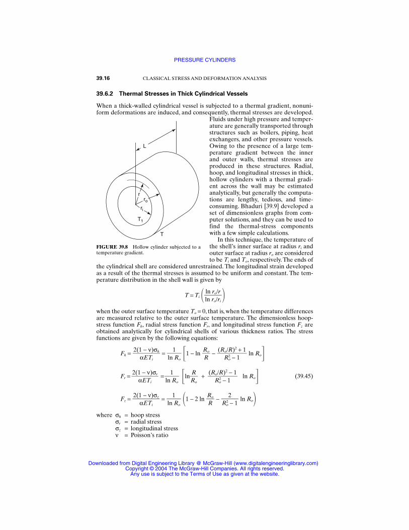
39.6.2 Thermal Stresses in Thick Cylindrical Vessels
When a thick-walled cylindrical vessel is subjected to a thermal gradient, nonuni-form deformations are induced, and consequently, thermal stresses are developed.
Fluids under high pressure and temper-ature are generally transported throughstructures such as boilers, piping, heatexchangers, and other pressure vessels.Owing to the presence of a large tem-perature gradient between the innerand outer walls, thermal stresses areproduced in these structures. Radial,hoop, and longitudinal stresses in thick,hollow cylinders with a thermal gradi-ent across the wall may be estimatedanalytically, but generally the computa-tions are lengthy, tedious, and time-consuming. Bhaduri [39.9] developed aset of dimensionless graphs from com-puter solutions, and they can be used tofind the thermal-stress componentswith a few simple calculations.
In this technique, the temperature ofthe shell’s inner surface at radius ri andouter surface at radius ro are consideredto be Ti and To, respectively.The ends of
the cylindrical shell are considered unrestrained. The longitudinal strain developedas a result of the thermal stresses is assumed to be uniform and constant. The tem-perature distribution in the shell wall is given by
T = Ti when the outer surface temperature To = 0, that is, when the temperature differencesare measured relative to the outer surface temperature. The dimensionless hoop-stress function Fh, radial stress function Fr, and longitudinal stress function Fz areobtained analytically for cylindrical shells of various thickness ratios. The stressfunctions are given by the following equations:
Fh = = 1 − ln − ln Ro
Fr = = ln + ln Ro (39.45)
Fz = = 1 − 2 ln − ln Rowhere σh = hoop stress
σr = radial stressσz = longitudinal stressν = Poisson’s ratio
2R2
o − 1RoR
1ln Ro
2(1 − ν)σzαETi
(Ro/R)2 − 1
R2o − 1
RRo
1ln Ro
2(1 − ν)σrαETi
(Ro/R)2 + 1
R2o − 1
RoR
1ln Ro
2(1 − ν)σhαETi
ln ro/rln ro/ri
39.16 CLASSICAL STRESS AND DEFORMATION ANALYSIS
ri
ro
T1
T
r
L
FIGURE 39.8 Hollow cylinder subjected to atemperature gradient.
PRESSURE CYLINDERS
Downloaded from Digital Engineering Library @ McGraw-Hill (www.digitalengineeringlibrary.com)Copyright © 2004 The McGraw-Hill Companies. All rights reserved.
Any use is subject to the Terms of Use as given at the website.
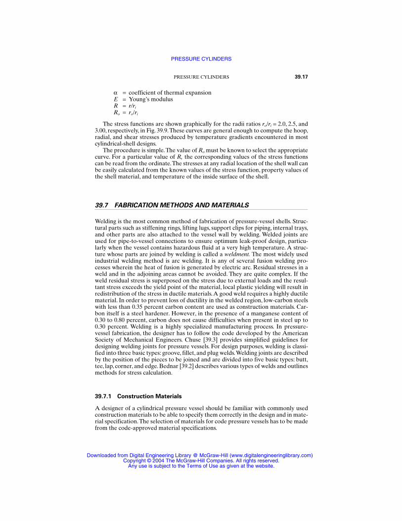
α = coefficient of thermal expansionE = Young’s modulusR = r/ri
Ro = ro/ri
The stress functions are shown graphically for the radii ratios ro/ri = 2.0, 2.5, and3.00, respectively, in Fig. 39.9.These curves are general enough to compute the hoop,radial, and shear stresses produced by temperature gradients encountered in mostcylindrical-shell designs.
The procedure is simple.The value of Ro must be known to select the appropriatecurve. For a particular value of R, the corresponding values of the stress functionscan be read from the ordinate.The stresses at any radial location of the shell wall canbe easily calculated from the known values of the stress function, property values ofthe shell material, and temperature of the inside surface of the shell.
39.7 FABRICATION METHODS AND MATERIALS
Welding is the most common method of fabrication of pressure-vessel shells. Struc-tural parts such as stiffening rings, lifting lugs, support clips for piping, internal trays,and other parts are also attached to the vessel wall by welding. Welded joints areused for pipe-to-vessel connections to ensure optimum leak-proof design, particu-larly when the vessel contains hazardous fluid at a very high temperature. A struc-ture whose parts are joined by welding is called a weldment. The most widely usedindustrial welding method is arc welding. It is any of several fusion welding pro-cesses wherein the heat of fusion is generated by electric arc. Residual stresses in aweld and in the adjoining areas cannot be avoided. They are quite complex. If theweld residual stress is superposed on the stress due to external loads and the resul-tant stress exceeds the yield point of the material, local plastic yielding will result inredistribution of the stress in ductile materials.A good weld requires a highly ductilematerial. In order to prevent loss of ductility in the welded region, low-carbon steelswith less than 0.35 percent carbon content are used as construction materials. Car-bon itself is a steel hardener. However, in the presence of a manganese content of0.30 to 0.80 percent, carbon does not cause difficulties when present in steel up to0.30 percent. Welding is a highly specialized manufacturing process. In pressure-vessel fabrication, the designer has to follow the code developed by the AmericanSociety of Mechanical Engineers. Chuse [39.3] provides simplified guidelines fordesigning welding joints for pressure vessels. For design purposes, welding is classi-fied into three basic types: groove, fillet, and plug welds.Welding joints are describedby the position of the pieces to be joined and are divided into five basic types: butt,tee, lap, corner, and edge. Bednar [39.2] describes various types of welds and outlinesmethods for stress calculation.
39.7.1 Construction Materials
A designer of a cylindrical pressure vessel should be familiar with commonly usedconstruction materials to be able to specify them correctly in the design and in mate-rial specification.The selection of materials for code pressure vessels has to be madefrom the code-approved material specifications.
PRESSURE CYLINDERS 39.17
PRESSURE CYLINDERS
Downloaded from Digital Engineering Library @ McGraw-Hill (www.digitalengineeringlibrary.com)Copyright © 2004 The McGraw-Hill Companies. All rights reserved.
Any use is subject to the Terms of Use as given at the website.
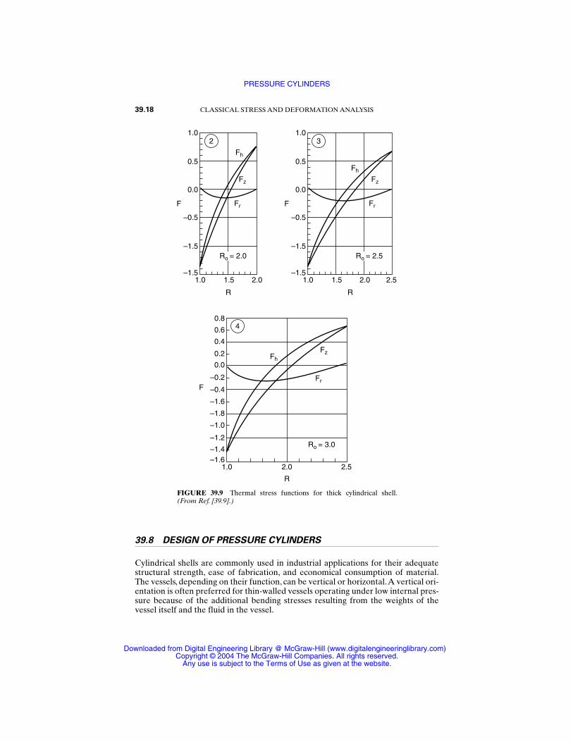
39.8 DESIGN OF PRESSURE CYLINDERS
Cylindrical shells are commonly used in industrial applications for their adequatestructural strength, ease of fabrication, and economical consumption of material.The vessels, depending on their function, can be vertical or horizontal.A vertical ori-entation is often preferred for thin-walled vessels operating under low internal pres-sure because of the additional bending stresses resulting from the weights of thevessel itself and the fluid in the vessel.
39.18 CLASSICAL STRESS AND DEFORMATION ANALYSIS
1.0
0.5
0.0
–0.5
–1.5
–1.51.0 1.5 2.0
F
R
Fr
Fz
Fh
1.0
0.5
0.0
–0.5
–1.5
–1.51.0 1.5 2.0 2.5
F
R
Fr
Fz
Fh
0.8
0.6
0.4
0.2
0.0
–0.2
–0.4
–1.6
–1.8
–1.0
–1.2
–1.4–1.6
1.0 2.0
R
2.5
Ro = 3.0
Fr
FzFh
F
4
32
Ro = 2.0 Ro = 2.5
FIGURE 39.9 Thermal stress functions for thick cylindrical shell.(From Ref. [39.9].)
PRESSURE CYLINDERS
Downloaded from Digital Engineering Library @ McGraw-Hill (www.digitalengineeringlibrary.com)Copyright © 2004 The McGraw-Hill Companies. All rights reserved.
Any use is subject to the Terms of Use as given at the website.
Cylindrical shells of such elastic materials as steels, nonferrous metals, and mostalloys that operate under internal pressures up to 10 MPa are fabricated mostly ofrolled and subsequently welded sheets. The joint connections of cylindrical shellsmade of copper or brass sheets are made by soldering with suitable solders. Cylin-drical vessels of steel operating under pressures greater than 10 MPa are commonlyfabricated of forged pieces that are heat-treated. Cylindrical shells of brittle materi-als for vessels operating under low internal pressures (approximately up to 0.8 MPa)are molded. Cast shells are usually fabricated with a bottom. In some cases, castshells are made of elastic metals and their alloys.
The fabrication of the cylindrical vessels by the rolling of sheets is a very commonmethod of manufacturing low- and medium-pressure (1.75 to 10.0 MPa) vessels.
Azbel and Cheremisinoff [39.1] give the following general guidelines for design-ing welded and soldered cylindrical shells:
1. The length of the seams should be minimized.2. The minimum number of longitudinal seams should be provided.3. Longitudinal and circumferential seams must be butt welded.4. All joints should be accessible for inspection and repair.5. It is not permissible to provide holes, access holes, or any opening on the seams,
especially on longitudinal seams.
Shell thicknesses of vessels operating under very low pressures are not designed;they are selected on the basis of manufacturing considerations. Durability is esti-mated from the available information regarding corrosion resistance of the material.The minimum thicknesses of a shell rolled from sheet metals are given as follows:carbon and low-alloy steel, 4 mm; austenite steel, 3.0 to 4.0 mm; copper, 2.5 to 3.0mm; and cast materials, 2.0 to 2.5 mm.
39.8.1 Design of Welded Cylindrical Shells
The structural design of cylindrical shells is based on membrane theory. In order toexpress the design relations in convenient form, it is necessary to (1) select thestrength theory best reflecting the material behavior, (2) consider the weakening ofthe construction induced by welding and other connections, (3) consider wall thin-ning as a result of corrosion effects, and (4) establish a factor of safety and allowablestresses.
The distortion-energy theory (see Chap. 28) gives the basic design stress as
σd = [σt2 + σ2
+ σr2 − 2(σtσ + σtσr + σσr)]1/2 (39.46)
where σt, σ, and σr = principal circumferential, longitudinal, and radial stresses,respectively. For a thin-walled cylindrical shell operating under an internal pressurepi, the radial stress is assumed to be equal to zero, and the longitudinal stress inducedin the shell is given by
σ = (39.16)
where di = inside diameter, and t = the thickness of the shell. The circumferentialstress induced in the shell is given by
pidi4t
PRESSURE CYLINDERS 39.19
PRESSURE CYLINDERS
Downloaded from Digital Engineering Library @ McGraw-Hill (www.digitalengineeringlibrary.com)Copyright © 2004 The McGraw-Hill Companies. All rights reserved.
Any use is subject to the Terms of Use as given at the website.
σt = (39.12)
When the deformation reaches plastic state, a definite amount of deformation energyis assumed (see Ref. [39.1]), and the value of the Poisson’s coefficient v is taken asequal to 0.5.
Substituting Eqs. (39.16) and (39.12) into Eq. (39.46) and assuming the value ofPoisson’s coefficient v = 0.5, the design stress can be expressed as
σd = 0.87 (39.47)
where ro = external radius of the shell. The external radius ro = do/2, where do =external diameter of the shell.
It is observed that according to the distortion-energy theory, considering thecombined effect of the longitudinal and tangential stresses, the design stress for plas-tic material is 13.0 percent less compared with the maximum value of the mainstress. The allowable stress σa is therefore given by
σa = (39.48)
And the thickness of the shell t is given by
t = (39.49)
Introducing the joint efficiency factor ηj and allowance factor tc for corrosion, ero-sion, and negative tolerance of the shell thickness, the following relation for designthickness is obtained:
td = + tc (39.50)
Azbel and Cheremisinoff [39.1], on the basis of similar analysis, give the followingdesign formula for the determination of shell thickness:
td = + tc (39.51)
where do/di ≤ 1.5.The proper selection of allowable stress to provide safe operation of a vessel is an
important design consideration. The allowable stress value is influenced by a num-ber of factors, such as (1) the strength and ductility of the material, (2) variations inload over time, (3) variations in temperature and their influence on ductility andstrength of the material, and (4) the effects of local stress concentration, impactloading, fatigue, and corrosion.
In shell design, the criterion of determining the allowable stresses in an environ-mentally moderate temperature is the ultimate tensile strength. The pressure-vesselcodes [39.3] use a safety factor of 4 based on the yield strength Sy for determining theallowable stresses for pressure vessels. The safety factor ηy is defined as
pidi2.3ηjσa − pi
pdo2.3σaηj
pdo2.3σa
pido2.3t
pirot
pidi2t
39.20 CLASSICAL STRESS AND DEFORMATION ANALYSIS
PRESSURE CYLINDERS
Downloaded from Digital Engineering Library @ McGraw-Hill (www.digitalengineeringlibrary.com)Copyright © 2004 The McGraw-Hill Companies. All rights reserved.
Any use is subject to the Terms of Use as given at the website.
ηy = (39.52)
It is known that for ductile metals, an increase in temperature results in an increasein ductility and a decrease in the yield-strength value. The allowable stress at highertemperatures can be estimated by using the following relation:
σa = (39.53)
where SyT = yield strength of the material at a given operating temperature.
Implied in the preceding analysis is an assumption that no creeping of the shellmaterial is involved. This is generally a valid assumption for ferrous metals underload at temperatures less than 360°C. However, at higher operating temperatures,the material creeps under load, and an increase in stress takes place with time. Theresulting stresses do not exceed the yield-strength values. It is to be noted that theyield point at high temperatures cannot generally be used as a criterion forallowance of the stressed state because creep of the material may induce failures asa result of the increased deformation over a long period of time.The basic design cri-terion for shells operating at moderate temperatures is the stability of size anddimensional integrity of the loaded elements. For a shell operating at higher tem-peratures, increase in size, which ensures that creep does not exceed a tolerablelimit, should be considered. When a loaded material is under creep, there is an asso-ciated relaxation of stress. The stress decreases over time as a result of plastic defor-mation. The creep rate is dependent on temperature and state of stress in the metal.Azbel and Cheremisinoff [39.1] discuss the effects of creep and stress relaxation onloaded shells and give a formula for determining the allowable stresses and safetyfactors on the basis of fatigue stress.
REFERENCES
39.1 D. S. Azbel and N. P. Cheremisinoff, Chemical and Process Equipment Design—VesselDesign and Selection, Ann Arbor Science Publishers, Ann Arbor, Michigan, 1982.
39.2 H. H. Bednar, Pressure Vessel Design Handbook, Van Nostrand Reinhold, New York,1981.
39.3 R. Chuse, Pressure Vessel—The ASME Code Simplified, 5th ed., McGraw-Hill, NewYork, 1977.
39.4 E. W. Comings, High Pressure Technology, McGraw-Hill, New York, 1956.
39.5 J. F. Harvey, Pressure Vessel Design: Nuclear and Chemical Applications, D. Van Nos-trand, Princeton, N.J., 1963.
39.6 B. L. Gatewood, Thermal Stresses, McGraw-Hill, New York, 1957.
39.7 D. Bergen, Elements of Thermal Stress Analysis, C. P. Press, Jamaica, N.Y., 1971.
39.8 J. N. Goodier, “Thermal Stress in Pressure Vessel and Piping Design, Collected Papers,”ASME, New York, 1960.
39.9 S. Bhaduri, “Thermal Stresses in Cylindrical Sheels,” Machine Design, vol. 52, no. 7,April 10, 1980.
39.10 J. H. Faupel and F. E. Fisher, Engineering Design, Wiley, New York, 1981.
SyT
ηy
Syσa
PRESSURE CYLINDERS 39.21
PRESSURE CYLINDERS
Downloaded from Digital Engineering Library @ McGraw-Hill (www.digitalengineeringlibrary.com)Copyright © 2004 The McGraw-Hill Companies. All rights reserved.
Any use is subject to the Terms of Use as given at the website.

PRESSURE CYLINDERS
Downloaded from Digital Engineering Library @ McGraw-Hill (www.digitalengineeringlibrary.com)Copyright © 2004 The McGraw-Hill Companies. All rights reserved.
Any use is subject to the Terms of Use as given at the website.