Embed Size (px)
Citation preview

İSTANBUL TECHNICAL UNIVERSITY GRADUATE SCHOOL OF SCIENCE
ENGINEERING AND TECHNOLOGY
M.Sc. THESIS
June 2016
Impervious Surface Estimation and Mapping via Remotely Sensed Techniques
Thesis Advisor: Assoc. Prof. Dr. Filiz BEKTAS BALCIK
Kaveh Khorshid
Department of Geomatics Engineering
Geomatics Engineering Programme


Department of Geomatics Engineering
Geomatics Engineering Programme
June 2016
İSTANBUL TECHNICAL UNIVERSITY GRADUATE SCHOOL OF SCIENCE
ENGINEERING AND TECHNOLOGY
Impervious Surface Estimation and Mapping via Remotely Sensed Techniques
M.Sc. THESIS
Kaveh KHORSHID
501121615
Thesis Advisor: Assoc. Prof. Dr. Filiz BEKTAS BALCIK


Geomatik Mühendisliği Anabilim Dalı
Geomatik Mühendisliği Programı
Haziran 2016
İSTANBUL TEKNİK ÜNİVERSİTESİ FEN BİLİMLERİ ENSTİTÜSÜ
Uzaktan Algılama Teknikleri İle Geçirimsiz Yüzey Tahmini ve Haritalanması
YÜKSEK LİSANS TEZİ
Kaveh KHORSHID
501121615
Tez Danışmanı: Doç.Dr. Filiz Bektas BALCIK


v
Thesis Advisor : Doç.Dr. Filiz Bektas BALCIK ..............................
İstanbul Technical University
Jury Members : Prof.Dr. Dursun Zafer Seker ..............................
İstanbul Technical University
Prof.Dr. Bulent Bayram ..............................
Yildiz Technical University
Kaveh-Khorshid, a M.Sc student of İTU Graduate School of Science Engineering
and Technology student ID 501121615, successfully defended the thesis entitled
“IMPERVIOUS SURFACE ESTIMATION AND MAPPING VIA REMOTELY
SENSED TECHNIQUES”, which he prepared after fulfilling the requirements
specified in the associated legislations, before the jury whose signatures are below.
Date of Submission : 5 May 2016
Date of Defense : 8 June 2016

vi

vii
To my dear family,

viii

ix
FOREWORD
I would like to take this opportunity to thank many people for their support and
contribute toward the completion of this dissertation. First, I would like to express my
sincere appreciation to my dear advisor, Assoc.Prof.Dr. Filiz bektas BALCIK, for her
patience, motivation, enthusiasm, immense knowledge and continuous guidance and
support throughout my program of study and this research work.
I would like to thank my father, who that support me not only during my MSc. thesis
but also during my whole life. Also I thank my mother for her great love and
encouragement. At the end, many thanks to my dear friends for their help and support.
May 2016
Kaveh KHORSHID
(Civil engineer)

x

xi
TABLE OF CONTENTS
Page
FOREWORD ............................................................................................................. ix
TABLE OF CONTENTS .......................................................................................... xi ABBREVIATIONS ................................................................................................. xiii LIST OF TABLES ................................................................................................... xv LIST OF FIGURES ............................................................................................... xvii
SUMMARY ............................................................................................................. xix ÖZET......... ............................................................................................................. xxiii
INTRODUCTION .................................................................................................. 1 ARTIFICIAL SURFACE ...................................................................................... 5
Artificial Surfaces Defined and Described ......................................................... 5 Development of Impervious Surfaces as an Environmental Indicator ............... 6
REMOTE SENSING OF ARTIFICIAL SURFACES ........................................ 9 Principles of Remote Sensing ............................................................................ 9
Electromagnetic Spectrum and Radiation ........................................................ 10 Electromagnetic Interaction with Earth’s Features Spectral Reflectance ........ 12 3.3.1 Built up reflectance ................................................................................... 13
Techniques for Mapping and Estimating Impervious Surfaces ....................... 16 3.4.1 Optical surveying and global positioning systems .................................... 17
3.4.2 Photographic interpretation ....................................................................... 17
3.4.3 Detailed maps ............................................................................................ 17
3.4.4 Population density ..................................................................................... 18 3.4.5 Image classification ................................................................................... 18
REMOTE SENSING IMAGE PROCESSING ................................................. 21 Digital Image .................................................................................................... 21 Remote Sensing Spectral Indices ..................................................................... 21
Built-up Indices ................................................................................................ 22 4.3.1 Normalised difference built-up index (NDBI) .......................................... 23
4.3.2 Normalized difference bareness index (NDBaI) ....................................... 24 4.3.3 Index-based built-up index (IBI) ............................................................... 25 4.3.4 Urban index (UI) ....................................................................................... 26
4.3.5 Enhanced built-up and bareness index (EBBI) ......................................... 27 Image Classification ......................................................................................... 28
Density Slicing ................................................................................................. 29 Accuracy Assessment ....................................................................................... 29
STUDY AREA , DATA AND CASE STUDY .................................................... 33 Study Area ....................................................................................................... 33 Data Used ......................................................................................................... 35 5.2.1 Remote sensing satellites .......................................................................... 35 5.2.2 Landsat system .......................................................................................... 36 5.2.3 Characteristics of Landsat ......................................................................... 36
5.2.3.1 Sensors and specifications.................................................................. 36

xii
Spectral Indices ................................................................................................ 40
5.3.1 Built-up area indices.................................................................................. 40 Mapping Impervious Surface and Bare Land ................................................... 49 Accuracy Assessment ....................................................................................... 54
CONCLUSIONS AND RECOMMENDATIONS ............................................. 61 REFERENCES ..................................................................................................... 65
CURRICULUM VITAE .......................................................................................... 71

xiii
ABBREVIATIONS
ANN : Artificial Neural Network
ASTER : Advanced Spaceborne Thermal Emission and Reflection Radiometer
BU : Built-Up
DN : Digital Number
EBBI : Enhanced Built-Up and Bareness Index
ER : Electromagnetic Radiation
EROS : Earth Resources Observation and Since
ETM : Enhanced Thematic Mapper
IBI : Index-based Built-up Index
MNDWI : Modified Normalized Difference Water Index
MSS : Multispectral Scanner system
NASA : National Aeronautics and Space Administration
NDBI : Normalized Difference Built-up Index
NDBaI : Normalized Difference Bareness Index
NIR : Near Infrared
OLI : Operational Land Imager
SAVI : Soil Adjusted Vegetation Index
SWIR : Short Wave Infrared
TIR : Thermal Infrared
TM : Thematic Mapper
TOA : Top of Atmosphere
UI : Urban Index
USGS : U.S. Geological Survey

xiv
xv
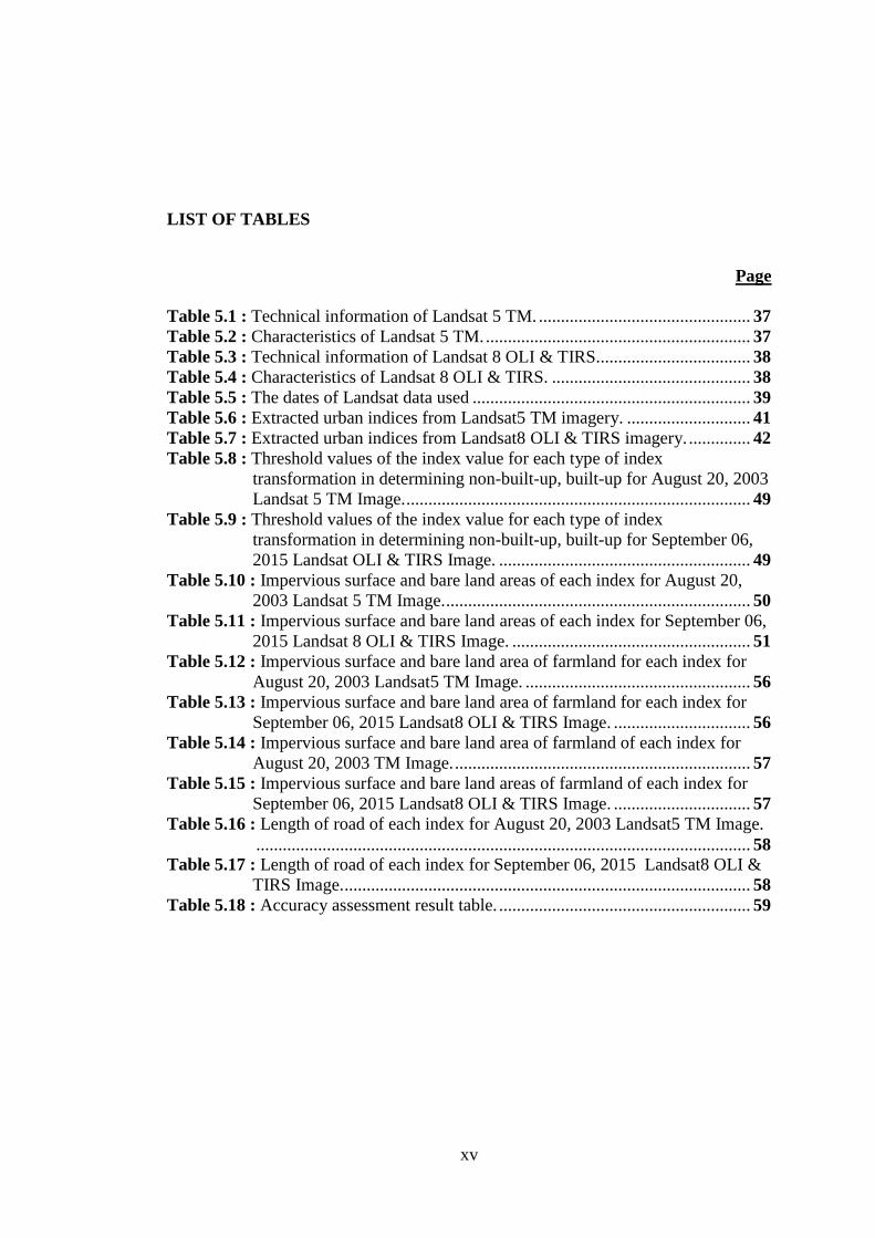
LIST OF TABLES
Page
Table 5.1 : Technical information of Landsat 5 TM. ................................................ 37 Table 5.2 : Characteristics of Landsat 5 TM. ............................................................ 37 Table 5.3 : Technical information of Landsat 8 OLI & TIRS................................... 38
Table 5.4 : Characteristics of Landsat 8 OLI & TIRS. ............................................. 38 Table 5.5 : The dates of Landsat data used ............................................................... 39
Table 5.6 : Extracted urban indices from Landsat5 TM imagery. ............................ 41 Table 5.7 : Extracted urban indices from Landsat8 OLI & TIRS imagery. .............. 42 Table 5.8 : Threshold values of the index value for each type of index
transformation in determining non-built-up, built-up for August 20, 2003
Landsat 5 TM Image. .............................................................................. 49 Table 5.9 : Threshold values of the index value for each type of index
transformation in determining non-built-up, built-up for September 06,
2015 Landsat OLI & TIRS Image. ......................................................... 49 Table 5.10 : Impervious surface and bare land areas of each index for August 20,
2003 Landsat 5 TM Image. ..................................................................... 50 Table 5.11 : Impervious surface and bare land areas of each index for September 06,
2015 Landsat 8 OLI & TIRS Image. ...................................................... 51 Table 5.12 : Impervious surface and bare land area of farmland for each index for
August 20, 2003 Landsat5 TM Image. ................................................... 56 Table 5.13 : Impervious surface and bare land area of farmland for each index for
September 06, 2015 Landsat8 OLI & TIRS Image. ............................... 56
Table 5.14 : Impervious surface and bare land area of farmland of each index for
August 20, 2003 TM Image. ................................................................... 57 Table 5.15 : Impervious surface and bare land areas of farmland of each index for
September 06, 2015 Landsat8 OLI & TIRS Image. ............................... 57 Table 5.16 : Length of road of each index for August 20, 2003 Landsat5 TM Image.
................................................................................................................ 58 Table 5.17 : Length of road of each index for September 06, 2015 Landsat8 OLI &
TIRS Image. ............................................................................................ 58 Table 5.18 : Accuracy assessment result table. ......................................................... 59

xvi

xvii
LIST OF FIGURES
Page
Figure 1.1 : Global distribution and density of constructed impervious ( Elvidge et
al, 2007) .................................................................................................... 2 Impervious surfaces vs pervious surfaces
(http://www.mdcoastalbays.org). ............................................................. 6
Figure 3.1 : Passive and active sensors (www.wikipedia.org).................................... 9
Figure 3.2 : Electromagnetic waves (www.shariqa.com) ......................................... 10
Figure 3.3 : Electromagnetic spectrum (Borges, 2008) ............................................ 11 Figure 3.4 : Spectral signature of the none urban features (Ramesh et al, 1995). .... 13 Figure 3.5 : (a) Spectral reflectance distribution in 450-900 nm wavelength region
for brick road surface; (b) Bituminous road surface; (c) Bituminous
rooftop surface (Ramesh et al, 1995). ..................................................... 14 Figure 3.6 : Comparison of spectral reflectance characteristics of brick, and
bituminous roads, and bituminous rooftops surfaces (Ramesh et al,
1995). ...................................................................................................... 15 Figure 4.1 : Digital image. ........................................................................................ 21
Figure 4.2 : Spectral profiles of six typical land covers for Landsat8 OLI & TIRS…
................................................................................................................ 25 Figure 4.3 : Density slicing. ...................................................................................... 29
Figure 4.4 : The error matrix (Foody, 2002) ............................................................. 30
Figure 5.1 : Location of the Istanbul ......................................................................... 35 Figure 5.2 : Landsat 5 TM - 20/08/2003 data (a) Frame 180/ 31 (b) Frame 180/ 32
(c) Mosaic and subsetted image. ............................................................. 40 Figure 5.3 : Flowchart of estimating impervious surface and bare land fraction in the
study. ....................................................................................................... 43 Figure 5.4 : NDBI images of Istanbul (a) August 20, 2003 (b) September 06,
2015........................................................................................................ 44 Figure 5.5 : NDBaI images of Istanbul (a) August 20, 2003 (b) September 06, 2015
................................................................................................................ 45 Figure 5.6 : UI images of Istanbul (a) August 20, 2003 (b) September 06, 2015..... 46 Figure 5.7 : EBBI images of Istanbul (a) August 20, 2003 (b) September 06,
2015........................................................................................................ 47 Figure 5.8 : IBI image of Istanbul (a) August 20, 2003 (b) September 06, 2015..... 48
Figure 5.9 : Validation of EBBI index image of August 20, 2003 classified as
impervious surface and bare land using Quickbird August 03, 2003
image as reference.................................................................................. 51
Figure 5.10 : The spatial distribution of impervious surfaces and bare lands is shown
for each type of index/remote sensing data transformation for August
20, 2003 Landsat5 TM Image: (a) EBBI, (b) IBI, (c) NDBI, (d) UI, (e)
NDBaI…………………………………………………………………. 52

xviii
Figure 5.11 : The spatial distribution of impervious surfaces and bare lands is shown
for each type of index/remote sensing data transformation for September
06, 2015 Landsat8 OLI & TIRS Image: (a) EBBI, (b) IBI, (c) NDBI, (d)
UI, (e) NDBaI………………………………………………………….. 53
Figure 5.12 : Missclassification of bare land as impervious surface in NDBI image
Landsat5 TM August 20, 2003 in contrast to Quickbird August 03, 2003
image....................................................................................................... 54 Figure 5.13 : Ataturk airport land cover extraction by urban indices……………… 55 Figure 5.14 : Farmland west of Istanbul (Quickbird)……………………………… 56
Figure 5.15 : Impervious surface and bare land area of farmland of each index for
August 20, 2003 TM Image…………………………………………… 57 Figure 5.16 : Impervious surface and bare land areas of farmland of each index for
September 06, 2015 Landsat OLI & TIRS Image…………………….. 57 Figure 5.17 : Road by the Buyukcavuslu (WorldView-3)………………………… 58

xix
IMPERVIOUS SURFACE ESTIMATION AND MAPPING VIA REMOTELY
SENSED TECHNIQUES
SUMMARY
Land cover and land use of earth has significantly been changed by unplanned and
uncontrolled expansion of urban areas throughout time and the increasing change by
the passing years, were verified by various studies. Only remote sensing from space,
can provide the global, repeatable, continuous observations of processes, needed to
understand the Earth system as a whole. Remote sensing data can be used in several
applications such as, meteorological data collection, change detection and land cover
mapping, urban planning, climate change, disaster monitoring and so on. One of the
important applications of remote sensing is to detect, monitor and map impervious
surfaces in urban areas. Impervious surfaces are present in many areas of the world.
The areas most affected by this change are developing countries and the metropolitan
cities, which are under pressures due to an unprecedented increase in population
growth and developments as the result of urbanization and industrialization.
Land Use and Land Cover (LULC) and Impervious Surface Area (ISA) are important
parameters for many environmental studies, and serve as an essential tool for decision
makers and stakeholders in Urban & Regional planning. Istanbul is among the cities
that is facing the problem of a large amount of land cover changes because of various
factors specifically urbanization and population growth. Urbanization phenomena with
all its advantages for people, causes the large portion of land cover and land use change
in mega cities such as Istanbul. Available medium spatial resolution satellite imagery,
in combination with Remote Sensing techniques, are very important sources in
analyzing the urban areas. Classification of Landsat images using remote sensing
indices are the mostly used and simple methodology for detecting and extracting the
impervious surface and bare land classes.
In this study, the Impervious surface area and bare land determination of Istanbul from
years, 2003 and 2015 were analyzed using different remote sensing indices such as UI

xx
(Urban Index), IBI (Index Based Built Up Index), NDBI (Normalized Difference
Built-Up Index), NDBal (Normalized Difference Bare Land Index) and EBBI
(Enhanced Based Built Up Index). Multitemporal data were acquired from freely
available LANDSAT 5 TM and LANDSAT 8 OLI & TIRS satellite in two different
dates (20-August-2003, 06-September-2015).
In the introduction part of the thesis, definition of remote sensing and a brief summary
of the topic are given. In the second chapter, general information about artificial
surface is provided. In the third chapter, the electromagnetic spectrum, radiation and
electromagnetic interaction with Earth’s features, spectral reflectance and remote
sensing of artificial surfaces are explained. In the fourth chapter, digital image
processing is defined and indices are explained.
In the application chapter, the study area Istanbul and the data used including satellite
data are defined. In this study, it is aimed to evaluate the impervious surfaces and bare
lands in the study area, using remote sensing indices; and to analyze the potential of
each urban index specially EBBI index since this study is among the first to apply this
index on a heterogenous urban area and finally to produce the impervious surface map
of Istanbul. With regard to the above objectives different built-up and bare soil indices
were applied to analyze impervious surface and bare soil and threshold values for three
categories as impervious surface, bare soil and others was decided by visual
interpratation and then dencity slicing was applied for producing thematic map of
Istanbul. Other category includes green areas, forest areas and water
surfaces. Accuracy assessment was calculated for each of indices to determine how
accurately the indices worked to solve classification problem of impervious surface
and bare lands in heterogenous urban areas by implementing visual interpretation,
digitizing for area and length, overall accuracy and Kappa statistics.
As the result of study, UI index has 90% overall accuracy for impervious surface,
EBBI index peresents 93% overall accuracy for bare land, IBI index has 84% overall
accuracy for impervious surface, NDBI index has 73% overall accuracy for impervious
surface and NDBaI has 88% overall accuracy for bare land. EBBI index shows the
highest impervious surface area of 121,421 ha and for the bare land NDBaI index
features highest area of 67,255 ha for Landsat 5 TM August 20, 2003 data. For Landsat
8 OLI & TIRS September 06, 2015 EBBI index shows 87% overall accuracy for
impevious surface, NDBaI index has 92% overall acuuracy for bare land, IBI index

xxi
shows 89% overall accuracy for bare land, NDBI has 86% overall accuracy for bare
land and UI has 87% overall accuracy for bare land. EBBI index presents the highest
impervious surface area of 137,406 ha and NDBaI Index confirms highest bare land
area of 56,508 ha.
It can be asserted that indices generated by utilizing the multispectral feature of
Landsat imagery, which has the long-term archive of satellite images, can be used for
determining the land cover/use changes. In addition, some recommendations for the
future research and the problems which encountered during analysis are outlined.

xxii

xxiii
UZAKTAN ALGILAMA TEKNİKLERİ İLE GEÇİRİMSİZ YÜZEY
TAHMİNİ VE HARİTALANMASI
ÖZET
Bu çalısmada iki farklı tarihte elde edilmiş farklı spektral çözünürlükte Landsat uydu
görüntülerinin “İstanbul” örneginde; geçirimsiz alanların ve boş alanların
belirlenmesinde kullanılabilirlikleri için uygulanabilecek farklı uzaktan algılama
indeksleri ele alınmıstır. Kullanılan yöntemler ile elde edilen yeni islenmis
görüntülerin performanslarının karşılaştırılması ile Istanbul için kullanılan indeksler
arasından en doğru sonuç veren indeksin belirlenmesi hedeflenmiştir.
Gerek ülkemizde gerek dünyamızda, şehir alanların yönetilmesi ve gelistirilmesi için
dogru ve güvenilir verilere ve veri elde etme yöntemlerine gereksinim duyulmaktadır.
Veri destegi ile çok amaçlı haritaların üretilmesi ve bu alanların sürekli izlenmesini
saglayacak teknolojilerin kullanımı gerekmektedir. Uzaktan algılama teknolojisi farklı
ölçekte, tekrarlı ve devamlı gözlemler ile yeryüzünü anlamak için kullanılan etkin bir
yöntemdir. Farklı çözünürlüklere sahip uzaktan algılanmış görüntüler meteorolojik
veri toplama, arazi örtüsü ve kullanımı haritalarının üretilmesi ve değişim tespiti, şehir
planlama, iklim değişimi, doğal afetlerin izlenmesi gibi çok sayıda uygulamada etkin
ve yaygın olarak kullanılmaktadır. Şehir alanlarında geçirimsiz yüzeylerin (yapay
yüzeylerin) belirlenmesi, izlenmesi ve değişimlerinin tespit edilmesi uzaktan algılama
teknolojisinin önemli uygulama alanları arasında bulunmaktadır. Geçirimsiz yüzeyler
şehir alanlarının büyük bir bölümünü kaplamaktadır. Geçirimsiz yüzeyler ve bunların
olumsuz etkileri en yaygın olarak şehirleşme ve endüstirileşme ve bunlara bağlı olarak
gözlemlenen hızlı nüfus artışlarının meydana geldiği gelişmekte olan mega şehirlerde
gözlenmektedir. Şehir alanlarının plansız ve kontrolsüz büyümesinden dolayı son
yıllarda meydana gelen arazi kullanımı ve arazi örtüsü değişimleri ve bunların çevresel
fakörler üzerindeki etkileri çok sayıda bilimsel çalışmada incelenmiştir.
Arazi kullanımı /örtüsü ve geçirimsiz yüzeyler çevresel çalışmalar ve bunların
sonuçlarını kullanan karar vericiler için önemli parametrelerdir. Orta çözünürlükte

xxiv
uydu görüntüleri ve uzaktan algıma teknikleri şehir alanlarının analizi ve sürdürülebilir
yönetimi için çok önemli kaynaklardır. Uzaktan algılama indeksleri ile uydu
görüntülerinin sınıflandırılması geçirimsiz yüzeylerin ve boş alanların tespit edilmesi
ve izlenmesi için yaygın olarak kullanılan etkili bir yöntem olarak kabul edilmektedir.
Bu arastırmada, özellikle 1980 yılı sonrasında hızlı nüfus artısı, sanayilesme ve buna
baglı olarak yerlesim alan artısı ve farklı arazi örtüsü degisimlerinin gözlemlendigi
Istanbul ili çalısma bölgesi olarak seçilmistir. Bu tez çalısmasında, İstanbul iline ait
geçirimsiz alanların ve boş alanların tespiti için farklı spektral özelliklere sahip
uzaktan algılama verilerinin performanslarını analiz etmek amacı ile ücretsiz olarak
elde edilebilen orta mekansal çözünürlüğe sahip Landsat 5 TM ve Landsat 8
OLI&TIRS görüntüleri kullanılmıstır.
Uygulamanın ilk asamasında, orta mekansal çözünürlüge sahip 20 Agustos 2003
tarihli Landsat 5 TM ve 6 Eylül 2015 tarihli Landsat 8 OLI& TIRS görüntüleri elde
edilmistir.
Bu Çalışmada, literatürde yaygın olarak kullanılan farklı uzaktan algılama indeksleri
ile Istanbul geçirimsiz alanlarının ve boş alanların belirlenmesi ve farklı indekslerin
performanslarının karşılaştırılması amaçlanmıştır. Çalışma kapsamında kullanılan
uzaktan algılama indeksleri UI (Urban Index (Şehir Indeksi)), IBI (Index Based Built
Up Index (Indeks tabanlı yapay alan indeksi)), NDBI (Normalized Difference Built-
Up Index (Normalleştirilmiş Fark Yapay Alan Indeksi)), NDBal (Normalized
Difference Bare Land Index (Normalleştirilmiş Fark Boş Alan Indeksi)) ve EBBI
(Enhanced Based Built Up Index (Zenginleştirilmiş Yapay Alan ve Boş Alan Indeksi)
olarak belirlenmiştir. Indekslerin tümü Landsat 5 TM ve Landsat 8 OLI & TIRS
görüntülerinin ilgili bantları kullanılarak hesaplanmıştır. Özellikle seçilen indeksler
arasında ısıl bant kullanılan tek indeks olan EBBI indeksi bu çalışma ile ilk defa
heterojen özelliklere sahip bir mega şehir alanında kullanılmıştır. Ayrıca görüntü
bantları kullanılarak hesaplanan farklı indekslerin kullanılması ile hesaplanan tek
indeks olma özelliği taşıyan IBI indeksi bu çalışmada hem Landsat 5 TM hem de yeni
nesil Landsat 8 OLI & TIRS görüntüsüne uygulanmıştır. Her indeks için görsel
yorumlama yöntemi ile eşik değerler üç farklı sınıf için (geçirimsiz yüzeyler, boş
alanlar ve diğer) belirlenmiştir. Belirlenen eşik değerler kullanılarak yoğunluk
dilimleme yöntemi ile Istanbul için tematik haritalar oluşturulmuştur. Farklı indekslere
ait performansların karşılaştırılması için doğruluk değerlendirmesi görsel yorumlama,

xxv
alan ve uzunluk hesaplamaları için sayısallaştırma, genel doğruluk ve Kappa istatistiği
hesaplamaları ile gerçekleştirilmiştir. İstanbul için Landsat 5 TM ve Landsat 8 OLI
&TIRS görüntüleri ile geçirimsiz yüzeylerin ve boş alanların doğru ve güvenilir olarak
belirlenebildiği indeksler belirlenmiştir. . Sonuç olarak, Landsat 5 TM (20 Agustos
2003) görüntüsü ile en yüksek genel doğruluk EBBI indeksi kullanılarak elde
edilmiştir. 2003 tarihli görüntü ile hesaplanan indeksler için genel doğruluk değerleri
geçirimsiz yüzeyler ve boş alanlar için karşılaştırıldığında EBBI indeksi kullanılarak
yüksek genel doğruluk boş alan için % 93, IBI indeksi kullanılarak yüksek genel
doğruluk geçirimsiz yüzeyler için % 84, NDBI indeksi kullanılarak yüksek genel
doğruluk geçirimsiz yüzey için % 73, UI indeksi ile yüksek genel doğruluk geçirimsiz
yüzeyler için % 90 ve NDBal indeksi ile yüksek genel doğruluk boş alan için % 88
olarak hesaplanmıştır. Landsat 8 OLI & TIRS (06 Eylül 2015) görüntüsü ile en
yüksek genel doğruluk NDBal indeksi kullanılarak % 90.3 olarak edilmiştir. 2015
tarihli görüntü ile hesaplanan indeksler için genel doğruluk değerleri geçirimsiz
yüzeyler ve boş alanlar için karşılaştırıldığında EBBI indeksi kullanılarak yüksek
genel doğruluk geçirimsiz alanlar için % 87, IBI indeksi kullanılarak yüksek genel
doğruluk boş alan için % 89, NDBI indeksi kullanılarak yüksek genel doğruluk boş
alan için % 86, UI indeksi ile yüksek genel doğruluk boş alan için % 87 ve NDBal
indeksi ile yüksek genel doğruluk boş alan için % 92 olarak hesaplanmıştır. Bu
çalışma ile uzaktan algılama indeksleri uzun ve sürekli zaman arşivine sahip orta
çözünürlüklü çok bantlı Landsat görüntüleri ile heterojen bir yapıya sahip Istanbul için
kabul edilebilir doğrulukta geçirimsiz yüzeylerin ve boş alanların belirlenmesinde
etkin olarak kullanılabileceğini gösteren bir altlık çalışma gerçekleştirilmiştir.

xxvi

1
INTRODUCTION
Land-Use and Land Cover (LULC) changes are among the most important factors for
environmental change such as deforestation, urbanization, climate change and natural
disaster management (Turner II et al, 1995). Urban areas have been expanding very
fast and rates of population growth in urban areas are higher than the overall population
growth in most countries. This happens because urban areas are the focus of economic
activities and transportation hubs (Masek et al, 2000). Urban land changes, referred to
as urban sprawl, have effects for the environmental and socio- economic sustainability
of communities (Xu, 2007 ). Accurate LULC maps are needed for urban planning and
natural resource issues like open space preservation, forest management, urban growth
and losses of farm or natural lands, these maps have to distinguish accurately features
of the built environment from vegetation in the area.
Impervious surfaces are anthropogenic features through which water cannot infiltrate
into the soil, such as roads, driveways, sidewalks, parking lots, rooftops, and so on. In
recent years, impervious surface has emerged not only as an indicator of the degree of
urbanization, but also a major indicator of environmental quality (Arnold and Gibbons,
1996). The total ISA of the world is estimated to be 579,703 km2. This is nearly the
same size as the country of Kenya (584,659 km2). The country with the most ISA is
China (87,182 km2) followed closely by the United States (83,881 km2), and India
(81,221 km2) (Elvidge et al, 2007) (Figure 1.1).
A requirement for the quantitative study of environmental issues caused by the
increasing impervious surface is to obtain detailed information of impervious surface
in an urban area. Knowledge on impervious surfaces, especially the magnitude,
location, geometry, spatial patterns and the perviousness-imperviousness ratio, is
significant to a range of issues and themes in environmental science (Weng, 2012).
Therefore, accurate impervious surface mapping in the urban areas has recently
attracted unprecedented attention from natural scientists throughout the world (Weng,
2012).

2
Figure 1.1 : Global distribution and density of constructed impervious
( Elvidge et al, 2007)
Istanbul as Turkey’s largest city and also biggest city in Europe by population within
city limits, has always been under pressure of rapid urbanization because of its
superiority in historic, culture and specifically for its economic opportunities (Balik
Sanli et al, 2008). Urbanization development and population growth resulted in drastic
changes in the land cover of Istanbul through centuries. Istanbul has been always
confronted the illegal housing problem (Keyder, 2005). Beside this moot point,
planned urbanization itself means the change in the land cover and somehow damages
to the nature of Istanbul. It is obvious that there is no stopping for urbanization
operation and land cover change that has resulted because of that, so the land managers
and people liable for the consequences of changes in land cover of the city should
develop new methods and practical techniques for decreasing negative effects caused
by urbanization as much as possible (Mundhe and Jaybhaye, 2014). Vegetation cover
decreasing and its after effects, problems related to climate change, increasing of
impervious lands are some of adverse impacts of urbanization and land cover change
processes (Jiang et al, 2015). For monitoring spatial changes that occurred through
years and planning to solve problems of land cover changes, the trend of change in
previous years should be studied and the future planning should be done by
considering this trend of change (Bellard et al, 2014). Today remotely sensed data by
satellites are among the most used data for such kind of studies (Song et al, 2014).
Image data files of freely available medium spatial resolution data of Landsat products
are reliable data for detecting and studying changes through years.

3
Mapping the impervious surfaces in urban areas is important because the existence of
these types of land can be used as an indicator of urban development and
environmental quality. The mapping process applies different remotely sensed data
and spectral values based on the land use category. Urban change detection in Istanbul
has been investigated by researchers previously ((Musaoglu et al, 2006), (Kaya and
Curran, 2006), (Balik Sanli et al, 2008), (Geymen and Baz, 2008)). For detecting the
changes, there are some methods. Classification is the method which was used by Van
Niel, (1995), Yuan et al. (2005), Coban et al. (2010) through the application of multi
temporal images of the specific area. In this method, the classes are separated and the
size of each class is determined. Another method is using the bare soil and built-up
indices which are graphical indicators used to detect the target such as impervious
surface and its magnitude and intensity. Chen et al. (2006) classified urban land uses
using several remote sensing indices in the Pearl River Delta of China with high
accuracy. Indices for mapping impervious surfaces in urban areas, such as the Urban
Index (UI) Kawamura et al. (1996), Bare soil index (BI) Rikimaru and Miyatake
(1997), Normalised Difference Built-Up Index (NDBI) Zha et al. (2003), Normalised
Difference Bareness Index (NDBaI) Zhao and Chen (2005), Index-based Built-Up
Index (IBI) Xu (2008), and Enhanced Built-Up and Bareness Index (EBBI) As-syakur
et al. (2012) have been employed in various studies.
The main objectives of this study are: (1) to understand the spectral reflectance
characteristics of impervious surfaces of Istanbul, (2) to explore the potential of
Landsat 5 TM and Landsat 8 OLI & TIRS imagery to detect and map the impervious
surface over the study area.
In the framework of this study, impervious Surface and bare land detection is being
analyzed using freely available Landsat 5 TM and Landsat 8 OLI & OLI data (2003,
2015) in Istanbul, Turkey. Several built-up, bare soil indices were examined and maps
were produces. Finally accuracy assessment showing the precision of this study was
examined.

4

5
ARTIFICIAL SURFACE
Artificial Surfaces Defined and Described
The phrase artificial surfaces or “impervious surfaces” is a relatively new and
descriptive expression used to characterize certain land cover types found in urban
areas. The term impervious generally refers to something that is impenetrable or that
does not allow entrance or passage through (Merriam Webster, 1994). Impervious
surfaces are anthropogenic features through which water cannot infiltrate into the soil,
such as roads, driveways, sidewalks, parking lots, rooftops, and so on. In recent years,
impervious surface has emerged not only as an indicator of the degree of urbanization,
but also a major indicator of environmental quality (Arnold and Gibbons, 1996). As a
result, surfaces that do not allow the penetration or passage of another substance can
be considered impervious surfaces. Specific to this research, impervious surfaces will
be defined as any surface that does not allow the natural infiltration of water.
In any urban area, many different land cover types constitute impervious surfaces, such
as paved roads, sidewalks, driveways, parking lots and rooftops. They are typically
land cover types constructed from impervious materials such as asphalt, concrete,
brick and stone. When these materials are applied to an area, they create an effective
seal against the infiltration of water resulting in impervious surfaces.
Generally, most of the impervious surface land cover types found in urban areas can
be categorized as belonging to either transportation (roads, sidewalks, driveways,
parking lots, etc.), or rooftop (residential housing, buildings, etc.). From these two
major categories, those attributed to transportation are typically the largest contributors
to total impervious area (Schueler, 1994) (Figure 2.1).

6
Impervious surfaces vs pervious surfaces
(http://www.mdcoastalbays.org).
Development of Impervious Surfaces as an Environmental Indicator
Impervious surfaces have become an important variable for determining the overall
environmental health of a watershed. The extent of their presence tends to have a
profound effect upon the natural processes that normally occur within watersheds. The
most obvious of these effects is the increase in volume of surface runoff during storm
events. As more and more of a watershed's area are covered with impervious surfaces,
the volume of surface runoff from that watershed also increases. This occurs primarily
because covering an area with impervious material tends to make it more
hydrologically active, meaning the area is sealed from infiltration and thereby
generates surface runoff. A study by Novotny and Chesters (1981) indicated surfaces
created from impervious materials such as asphalt or concrete, the predominant
impervious material in urban areas, are nearly 100 percent hydrologically active.
The magnitude, location, geometry and spatial pattern of impervious surfaces, and the
pervious–impervious ratio in a watershed have hydrological impacts. Although land
use zoning emphasizes roof related impervious surfaces, transport-related impervious
surfaces could have a greater impact. The increase of impervious cover would lead to
the increase in the volume, duration, and intensity of urban runoff (Weng, 2012).
Watersheds with large amounts of impervious cover may experience an overall
decrease of groundwater recharge and baseflow and an increase of stormflow and flood
frequency (Brun and Band, 2000). Furthermore, imperviousness is related to the water

7
quality of a drainage basin and its receiving streams, lakes, and ponds. Increase in
impervious cover and runoff directly impact the transport of non-point source
pollutants including pathogens, nutrients, toxic contaminants, and sediment (Hurd and
Civco, 2004).
As discussed earlier, the definition and description of impervious surfaces for this
research was one that does not allow for the infiltration of water and can primarily be
categorized as belonging to either a transportation or rooftop land cover type.
Additionally, they are mainly a constructed surface that represents the imprint of land
development on the landscape. As the process of land development begins, impervious
surfaces are added in the forms of homes and driveways, shopping centers and parking
lots, streets and highways. Eventually, as various forms of impervious surfaces are
added, rural landscapes are replaced with urban communities. In effect, impervious
surfaces are a cultural by product of how urban communities are organized, stimulated
and protected. Because of the significant increases in impervious surfaces and
urbanization that has occurred during the last 50 years, it is intuitively rational that
many investigators such as Arnold and Gibbons (1996), Schueler (1994) and Sleavin
et al. (2000) refer to urban development as being synonymous with increases in
impervious surfaces.
Although increases in impervious surfaces can be correlated with increases in
urbanization, it is conceptually more important to recognize that impervious surfaces
are the common variable to many of the aforementioned effects on environmental
processes. This has led Schueler (1994) to advocate the use of impervious surfaces as
a unifying theme to help assess, mitigate and manage aquatic ecosystems. Similarly,
Arnold and Gibbons (1996) describe impervious surfaces as a valuable tool for both
protecting and managing water resources. In areas where few records or little detailed
information is available, they hypothesize impervious surfaces might be the most cost
effective and feasible parameter for addressing issues related to water resources. They
attribute this value to two major factors, the first of which is impervious surfaces are
integrative. This means a more uniform and consistent analysis can be reached about
water resources because inherent complexities associated with specific environmental
processes can be avoided.
The second factor is impervious surfaces are measurable (Arnold and Gibbons 1996).
This means its physical size or area can be determined and short of being modified or

8
destroyed, its results, once measured, are reproducible. Therefore, depending on the
size of the area considered and purpose for which it is to be applied, a wide range of
techniques exists for the measuring of impervious surfaces.

9
REMOTE SENSING OF ARTIFICIAL SURFACES
Principles of Remote Sensing
Remote sensing is the science of obtaining information about objects from a distance
and not being in contact with the object of interest. Information is gathered by the
processes of recording, measuring and interpreting of the imagery, derived typically
from aircrafts or satellites (Jensen, 2009).
Remote sensors can be either passive or active (Figure 3.1). Passive sensors record
radiation that is reflected from Earth’s surface, where the sun plays the role of
providing an energy source and illuminates the target. Because of this, passive sensors
can only be used to collect data during daylight hours; however, active sensors emit
signals to the Earth’s surface and record the backscattered or reflected signals.
Figure 3.1 : Passive and active sensors (www.wikipedia.org)

10
The radiation from the sun or satellite system incident upon the Earth’s surface causes
three different interactions with objects: It can be absorbed, transmitted or reflected.
The reflected energy is the most useful one in remote sensing applications. Reflection
occurs when a ray of light is redirected as it strikes a non-transparent surface.
Transmission of radiation occurs when radiation passes through a substance without
significant attenuation. Absorption occurs when all the electromagnetic radiation is
absorbed by objects on the Earth’s surface and converted into the other form of energy
or reradiated at a larger wavelength (Joseph, 2005) .
Electromagnetic Spectrum and Radiation
Electromagnetic wave’s energy transports energy through space in the form of periodic
disturbances of electric and magnetic fields (Figure 3.2). All electromagnetic waves
travel through space at the same speed, c=2.99792458 × 10⁸ m/s, commonly known
as the speed of light. An electromagnetic wave is characterized by a frequency and
wavelength.
These two quantities are related to the speed of light by the equation:
Speed of light = frequency × wavelength (3.1)
Figure 3.2 : Electromagnetic waves (www.shariqa.com)
Light is a particular type of electromagnetic radiation that can be seen and sensed by
the human eye, but this energy exists at a wide range of wavelengths. The micron is
the basic unit for measuring the wavelength of electromagnetic waves. The spectrum
of waves is divided into sections based on wavelength (Figure 3.3). The shortest waves
are gamma rays, which have wavelengths of 10e-6 microns or less. The longest waves
are radio waves, which have wavelengths of many kilometres. The range of visible

11
region consists of the narrow portion of the spectrum, from 0.4 microns (blue) to 0.7
microns (red) (Campbell, 1996).
Figure 3.3 : Electromagnetic spectrum (Borges, 2008)
Electromagnetic radiation is reflected or absorbed mainly by several gases in the
Earth’s atmosphere; among the most important ones are water, carbon dioxide and
ozone. Some radiation, such as visible light, largely passes (transmitted) through the
atmosphere. These regions of the spectrum with wavelengths that can pass through
atmosphere are referred to as “atmospheric window “. Some microwaves can even
pass through clouds, which make them the best wavelength for transmitting satellite
communication signals (Elachi and Van Zyl, 2006).
Electromagnetic radiation could be redirected due to the presence of particles and
gasses in the atmosphere; in this case, three different scattering mechanisms can occur:
Rayleigh scattering: It happens when the wavelength of the radiation is smaller than
the particles in atmosphere such as dust and oxygen molecules.
Mie scattering: It happens when the particles in the atmosphere are almost the same
size as the wavelength of radiation. Smoke, dust and water vapour are the common
cause of Mie scattering.
Nonselective scattering: It happens when particles are larger than the wavelength of
radiation; in this case, all wavelengths scatter almost equally. Water droplets and large
dust particles can cause this type of scattering.

12
Electromagnetic Interaction with Earth’s Features Spectral Reflectance
Objects having different surface features reflect or absorb the sun’s radiation in
different ways. The reflectance properties of an object depend on the particular
material, its physical and chemical state (e.g. moisture) and the surface roughness as
well as the geometric circumstances (e.g. incidence angle of the sunlight). The most
important surface features are colour, structure and surface texture.
The amount of energy reflected from the surfaces is usually expressed as a percentage
of the amount of energy striking the objects. Reflectance is 100% if all of the light
striking and object bounces off and is detected by the sensor. If none of the light returns
from the surface, reflectance is said to be 0%. In most cases, the reflectance value of
each object for each area of the electromagnetic spectrum is somewhere between these
two extremes.
Across any range of wavelengths, the percent reflectance values for landscape features
such as water, sand, roads, forests, etc. can be plotted and compared. Such plots are
called “spectral response curves” or “spectral signatures”. Differences among spectral
signatures are used to help classify remotely sensed images into classes of landscape
features since the spectral signatures of like features have similar shapes. The figure
below shows differences in the spectral response curves for main features (Figure 3.4).
Spectral information, recorded by a sensor can be extracted from the spectral
signatures. Hyperspectral sensors have much more detailed signatures than
multispectral sensors, and thus provide the ability to detect more subtle differences in
aquatic and terrestrial features (Curran, 1985).

13
Figure 3.4 : Spectral signature of the none urban features (Ramesh et al, 1995).
3.3.1 Built up reflectance
In urban areas, impervious surfaces are made up of different kinds of materials. The
maintenance of these surfaces, especially in metropolitan cities, is difficult. Now, with
advancements in digital remote sensing data analysis techniques and with the
availability of high resolution imagery, the assessment and evaluation of the status of
these surfaces can be done on a routine basis. Remote sensing can be very useful in
urban planning and management. This is only possible if we have a-priori information
about the spectral signature of these surfaces. Urban area reflectance is a function of
material properties of various types of impervious surfaces such as brick, mud, and
bituminous roads and bituminous rooftops (Ramesh et al, 1995).
Brick Road: The brick road consists of man-made light red c1in-baked bricks. Figure.
3.5a presents the spectral reflectance curve for the brick road surface. This figure
shows the direct relationship of reflectance to wavelength in the spectral region; i.e.,
the reflectance continuously increases with the wavelength. The obtained data points
are depicted by error bars (standard error from the mean) and the spectral reflectance
curve is drawn as the best fit curve for these data points. The value of spectral
reflectance is minimum (0.28) at the 485 nm wavelength and maximum (0.50) around
the 850 nm wavelength range (Ramesh et al, 1995).

14
Figure 3.5 : (a) Spectral reflectance distribution in 450-900 nm wavelength region for
brick road surface; (b) Bituminous road surface; (c) Bituminous rooftop
surface (Ramesh et al, 1995).
Bituminous Road: This surface is a very dark brownish-black color. Fig. 3.5(b) shows
the spectral reflectance properties for this surface. The data points are shown by error
bars (standard error from the mean) and the curve is drawn as the best fit for these data
points. This figure shows the direct relationship between reflectance and wavelength.
The reflectance shows a very small variation with the wavelength in the considered
wavelength range, with minimum value (0.18) at the 485 nm wavelength and
maximum value (0.25) around the 850 nm wavelength. In the visible range (450-700
nm), the reflectance is low because of the very dark coloured surface. In the near
infrared range (700-850 nm), the reflectance is low (but relatively higher than that in
the visible range). This may be due to the surface's roughness (as absorbance is more
for rough surfaces) and its other complex parameters (Fig. 3.5(b)).

15
Bituminous Rooftops: This is a dark reddish-brown surface and is relatively lighter
in color than the bituminous road. The composition and proportion of the construction
material used in the rooftop is different from that of the road and, hence, the difference
in color. Fig. 3.5(c) shows the spectral reflectance characteristics of the bituminous
rooftop. The data points are shown by the error bars (standard error from the mean)
and the spectral reflectance curve is drawn as the best fit curve for the obtained data
points. The reflectance is directly related to the wavelength in the considered
wavelength range. In this case, the reflectance shows small variation with the
wavelength but the variation is certainly more than that of the bituminous road. The
minimum reflectance (0.20) is observed at the 485 nm central wavelength and the
maximum reflectance (0.32) is observed around the 850 nm central wavelength. The
low reflectance in the visible region is because of the dark colored surface. The
relatively higher reflectance in the near-infrared region may be attributed to surface
roughness, type of construction material, and other complex parameters The low
reflectance in the visible region is because of the dark colored surface.
Figure 3.6 : Comparison of spectral reflectance characteristics of brick, and bituminous
roads, and bituminous rooftops surfaces (Ramesh et al, 1995).
Figure 3.6 shows the spectral reflectance curves for brick, bituminous roads, and
bituminous rooftop surfaces. These surfaces possess reflectance profiles typical of
man-made materials; i.e., generally increasing reflectance with increasing wavelength.

16
The reflectance curves of these surfaces are similarly shaped, and differ only in their
relative positions. The properties of brick road surface show contrast with those of the
bituminous road and rooftop surfaces and can be easily distinguished from the other
two surfaces in the entire wavelength range. Brick road surfaces also present
contrasting properties in the entire wavelength range and can be very easily
distinguished from each other. The reflectance pattern for the bituminous road and
rooftop is less distinctive, but these two can be differentiated from each other in the
red region of the visible spectrum (around the 650 nm wavelength).
Brick road surfaces possess a higher reflectance than those of the other two bituminous
surfaces, both in the visible and near-infrared regions of the spectrum. The brick road
has higher reflectance values than the other two bituminous surfaces because of its
brick-red color, which is relatively lighter than the dark brownish-black of the
bituminous road and dark reddish-brown of the rooftops. In the near-infrared region,
brick road surfaces show a relatively higher reflectance because of their color,
compositional differences and so on.
The bituminous road has a relatively lower spectral reflectance than that of the rooftop,
throughout the considered wavelength range, because of differences in color,
composition of the construction material, and surface roughness, and other complex
differences between the bituminous road and the airstrip. The bituminous road is
relatively darker than the rooftop.
Techniques for Mapping and Estimating Impervious Surfaces
A discussion of the wide range of techniques used to map and estimate impervious
surfaces will be presented in this section. Throughout the discussion, individual
techniques will be identified and described along with any specific advantages or
disadvantages associated with the technique for determining impervious surfaces. The
phrase “measurement of impervious surfaces” can be appropriately applied only in the
first technique described; the remaining techniques use methodical estimation. This is
primarily due to the aerial extents and amounts of impervious surfaces in many of the
studies. As study area size and amounts of impervious surfaces increase, it becomes
more difficult to perform a direct and quantifiable measurement.

17
3.4.1 Optical surveying and global positioning systems
The first method involves the physical measurement and quantification of area for all
impervious surfaces by either a traditional optical ground-based survey technique or
through the use of a global positioning system (GPS). According to Sleavin (1999),
optical surveying and GPS are the most accurate techniques; however, both require
extensive fieldwork and considerable man-hours to record geographic locations for all
roads, buildings, parking lots, sidewalks, etc. As a result most investigators consider
these techniques prohibitively cost effective, especially when measuring impervious
surfaces in large study areas.
3.4.2 Photographic interpretation
Photo interpretation uses aerial photography for estimating impervious surfaces.
Draper and Rao (1986), Harris and Rantz (1964), and Saurer et al. (1983) used photo
interpretation in their respective studies and considered it to be one of the most
accurate methods for determining impervious surfaces estimates. However, similar to
optical surveying and GPS, photographic interpretation can be time consuming and
very expensive. These issues are evident in the cost and operation of sophisticated
equipment such as aircraft and navigational instruments along with the skill level of
experienced individuals needed to use such equipment. This is why Sleavin (1999)
suggests that determining impervious surfaces from aerial photography is only
practical for small study areas (i.e., town-level or sub-regional watershed).
3.4.3 Detailed maps
Estimating impervious surfaces employs the use of detailed maps. Investigators such
as Martens (1968), Southard (1987), and Spencer and Alexander (1978) have all
attempted to extract impervious surfaces estimations from detailed maps by overlaying
them with grid frames from which to identify and quantify impervious surfaces.
However, because maps are mere representations or models of reality, the
identification and estimation of impervious surfaces is limited to the types of
information and level of detail the maps display. This level of detail, generally referred
to as scale, can be defined as the proportional distance between what is represented on
the map versus what is reality (Avery and Berlin, 1992). A small-scale map covers a
large geographic area with less detail as compared to a large-scale map covering a
smaller geographic area with more detail. As a result, the ability to extract accurate

18
impervious surfaces estimates from detailed maps is a process that is highly dependent
on the information represented and the scale.
3.4.4 Population density
A more indirect approach of estimating impervious surfaces is in using population
densities. Stankowski (1972) developed a quantitative index of urban land use
characteristics that could then be applied to water resource analyses. From his results,
Stankowski suggested population density was the only independent variable needed to
empirically estimate proportions of impervious surfaces associated with different
degrees of urban development. He developed and used correlation values between
population density and the proportions of land use in each of six urban land use
categories. From those values, he weighted his land use categories by the average
percentage of impervious surfaces found in each land use category. Using these
weighted correlation values the amount of impervious surfaces from a particular study
area could then be estimated. Although somewhat limited by inherent averaging
processes, this approach was offered as a rapid and inexpensive technique for
generating qualitative indices about urbanization and impervious surfaces.
3.4.5 Image classification
A fifth method for estimating impervious surfaces is the classification of remotely
sensed satellite data. The general process entails the collection of reflected
electromagnetic radiation from the earth’s surface to sensors onboard a satellite.
Depending upon the satellite, there are differences in the number of bands, individual
bandwidths, and spatial resolutions that sensors onboard various satellites are able to
detect and collect. Once the satellite data is collected it can be processed, formatted
and geo-rectified for analysis in a digital environment. Image classification operations
can then be performed.
Conceptually, the objective of digital image classification is to replace a subjective,
visual analysis process with a more objective, quantitative technique for automating
the identification of features in a scene. This procedure normally involves the analysis
of multispectral image data and the application of statistically based decision rules for
determining the feature identity of each pixel in an image. Ultimately, it is the intent
of the image classification process to categorize all pixels in a digital image into one
of several land use/land cover classes or “themes” (Lillesand et al, 2014).

19
As an early investigation into the potential of image classification, Toll (1984)
evaluated Landsat MSS and TM data for discriminating between different land cover
types. He noted higher levels of accuracy were achieved using Landsat TM data than
the older Landsat MSS data for classifying certain urban land cover types. Prior to his
investigation, there had been very few studies conducted that used remotely sensed
satellite data to classify urban land cover types. The lack of interest for classifying
urban features was due to the coarse spatial resolution (79-82 meters) of Landsat MSS
and the relative newness of the digital image classification technique.
However, with the improved spatial resolution of Landsat TM (30 meters), a new
interest for studying urban land cover was generated. Specific to this research, Plunk,
Morgan, and Newland, (1990) used the higher spatial resolution of Landsat TM to
classify impervious surfaces from an urban area near Fort Worth, Texas. Their results
indicated an 85.1 percent accuracy level for classifying impervious surfaces. Although
both studies reported improved accuracies for classifying certain urban feature types,
the authors indicated total impervious surfaces were often underestimated because of
the spatial complexity and heterogeneity of many urban land covers.
After reviewing these techniques in this section, it was concluded that mapping process
applies different remotely sensed data and spectral values based on the land use
category. Therefore image classification using remote sensing indices was the
technique chosen for this study. This was largely due to constraints in available data
and manpower, but ultimately the determination is to develop a practical means by
which urban areas could quantify impervious surfaces in a cost effective and timely
fashion with reasonable expertise.

20

21
REMOTE SENSING IMAGE PROCESSING
Digital Image
Objects in the real scene can be represented by a two-dimensional image. The images
can be divided in two categories, analogue and digital. Aerial photographs are
examples of analogue images while satellite images acquired using electronic sensors
are examples of digital images. A digital image is consisting of two-dimensional arrays
of pixels, which are the picture elements and represent a square area on Earth’s surface
that is a measure of sensor’s ability to resolve the objects of different sizes (Figure
4.1). Each pixel has brightness value, which is also called as intensity value in the
digital image. Intensity value usually is a single number that represents the brightness
of the pixel such as the solar radiance in a given wavelength band reflected from the
ground, emitted infrared radiation or backscattered radar intensity. The most common
pixel format is the byte images, where this number is stored as an 8-bit integer giving
a range of possible values from 0 to 255. Typically, zero is taken to be black and 255
is taken to be white. Values in between, make up the different shades of grey.
Figure 4.1 : Digital image.
Remote Sensing Spectral Indices
Spectral indices are the combinations of spectral bands at two or more wavelengths
that indicate relative abundance of features of interest. There are various types of
indices with different arithmetic formula used for different cases according to the
characteristics of features and purpose of study.

22
The indices were progressed in four different stages. The first indices are those
developed from simple band ratios and used for inferring the spectral properties of
vegetation through its growing period. The second stage is referred to the development
of indices designed to reduce the impacts of the background such as soil response. The
third indices are developed to compensate for the effects of atmospheric distortion.
The fourth and final stage of development procedure refers to the new spectral indices
development different from vegetation health. Indices that are used for burned area
assessment and fire severity are in the last developed group of indices (Harris et al,
2011). By applying the spectral indices to remotely sensed data, the sensitivity of
certain surface properties is maximized. Furthermore, the indices are capable of
normalizing or reducing effects due to sun angle, viewing angle, the atmosphere,
topography, instrument noise, etc. to make consistent spatial and temporal
comparisons possible (Jensen, 2009).
Built-up Indices
Remote sensing imagery can be used to separates urban lands from non-urban lands,
but, this may not produce satisfactory accuracy because of spectral confusion of the
heterogeneous urban built-up land class. Many studies have been done in combined
classification methods to improve the extraction of the urban built-up lands (Xu, 2005).
Transformation enhancement, one of the image - processing techniques, calculates
new values for each image pixel, based not only on the values within a particular
spectral band but also on some function of values in other spectral bands (Karen,
2008). Vegetation indices are ratios of bands that are designed to numerically separate
or stretch the pixel value of different features in the image. Many indices have been
developed that implement various band combinations. They use the distinctive feature
of leaf chlorophyll absorption (maximum at about 0.69 μm) and lack of absorption in
the adjacent near infrared region (at 0.85 μm) to isolate different features. The outcome
is a strong absorption contrast in the 0.65 - 0.85 μm wavelength interval (Liwa, 2006
). Vegetation indices utilises this contrast through the combinations of bands red/near-
infrared reflectance. There are a number of vegetation indices, such as the Normalized
Difference Vegetation Index (NDVI), that are function of the visible bands of
multispectral data and the near infrared bands. It has been determined that these indices
often give a very simple and fast interpretation of Landsat satellite data in terms of
23
vegetation health. Likewise, there are other indices using different spectral bands that
may be calculated to allow more efficient interpretation of features (Kemp, 2008).
The mapping process applies different remotely sensed data and spectral values based
on the land use category. Land use mapping primarily employs the multispectral
classification method; however, there are other methods that also utilise the application
of the remote sensing index. Chen et al. (2006) classified urban land uses using several
remote sensing indices in the Pearl River Delta of China with high accuracy. The most
popular indices which are relatively good for mapping the impervious surface and bare
land in urban areas, such as the Normalised Difference Built-Up Index (NDBI) Zha et
al. (2003), Index-based Built-Up Index (IBI) Xu, (2008), Urban Index (UI) Kawamura
et al. (1996), Normalised Difference Bareness Index (NDBaI) Zhao and Chen (2005),
and Bare soil index (BI) Rikimaru and Miyatake (1997), Enhanced Built-Up and
Bareness Index (EBBI) As-syakur et al. (2012) have been employed in various studies.
The IBI, NDBI, UI, and EBBI are indices for quickly mapping impervious surface and
bare land areas. In contrast, the NDVI is a well-known spectral index for rapidly
mapping the distribution of vegetation and a variety of conditions over land surfaces.
Previously, Braun and Herold (2004) applied NDVI for mapping the impervious area
of an urban area of Germany.
In the following built-up and bare land indices which was used in this study for Landsat
5 TM are explained and presented in Table 5.6 and for Landsat 8 OLI & TIRS in Table
5.7.
4.3.1 Normalised difference built-up index (NDBI)
Zha et al. (2003) suggested that spectral disparity is the largest in bands 3, 4 and 5 of
landsat 5 TM. An examination of the minimum, maximum and standard deviation of
each of the covers in the seven TM bands confirms the same conclusion. Namely, these
values are most distinctive from one another for each cover in bands 3, 4 and 5.
Therefore, they are the most useful bands from which some of the land covers may be
potentially differentiated spectrally. Rivers and lakes have a similar shape of profile.
Their Digital Number (DN) value is markedly lower in the fourth and fifth bands. They
experience a sharp rise in reflectance in band 6, but a low reflectance in band 7. The
curve for rivers lies above that for lakes because they are laden with more silt. A close
look reveals that except for barren, vegetation (woodland and farmland) has a higher

24
reflectance on band 4 than other covers. Moreover, its value on band 4 still exceeds
those on band 3. By comparison, all the non-vegetative categories have a smaller DN
on band 4 than 3. Therefore, the subtraction of band 3 from band 4 will result in
positive DNs for vegetation pixels only. The aforementioned relationships exist for the
minimum and maximum DNs as well . This outcome allows broad vegetative covers
to be distinguished easily. This processing is commonly referred to as NDVI .
NDVI = (Band 4−band 3)/(band 4+band 3) (4.3)
In order to facilitate the subsequent processing, the derived NDVI image was recoded
with 254 for all pixels having positive indices (vegetation) and 0 for all remaining
pixels of negative indices. Impervious surface areas and barren land experience a
drastic increment in their reflectance from band 4 to band 5 while vegetation has a
slightly larger or smaller DN value on band 5 than on band 4. This pace of increment
greatly exceeds that of any other covers. The minimum and maximum DNs in band 4
are much smaller than those in band 5 for the same cover. The standardized
differentiation of these two bands (equation 4.4) will result in close to 0 for woodland
and farmland pixels, negative for waterbodies, but positive values for impervious
surface pixels, enabling the latter to be separated from the remaining covers.
NDBI=(band 5 − band 4)/(band 5 + band 4) (4.4)
4.3.2 Normalized difference bareness index (NDBaI)
Normalized Difference Bareness Index (NDBaI) was first introduced by Zhao and
Chen in 2004. This index is based on significant differences of spectral signature in
the near-infrared (band 5 landsat 5 TM) between the bare-soil and the backgrounds.
However, it showed little difference between impervious surface areas and bare-soil
areas in band 5 (Figure 4.2) (Zhao and Chen, 2004). Figure 4.2 suggests that further
consideration of the visible may be necessary to determine the vegetation areas. It is
effective in distinguishing bare-soil from similarly impervious surface and vegetation.

25
Figure 4.2 : Spectral profiles of six typical land covers for Landsat8 OLI & TIRS
𝑁𝐷𝐵𝑎𝐼 =𝐵𝑎𝑛𝑑5−𝐵𝑎𝑛𝑑6
𝐵𝑎𝑛𝑑5+𝐵𝑎𝑛𝑑6 (4.5)
4.3.3 Index-based built-up index (IBI)
An urban area is a complex ecosystem composed of heterogeneous materials.
Nevertheless, based on some generalizing features, Ridd (1995) could still divide the
urban ecosystem into three components, green vegetation, impervious surface material
and exposed soil, and accordingly created a V-I-S model.
Consequently, the urban land-use was grouped into three other generalizing categories:
built-up land, vegetation and open water. Based on these three components, three
thematic indices, the normalized difference built-up index (NDBI), the soil adjusted
vegetation index (SAVI) and the modified normalized difference water index Xu
(2006), were selected to represent the three major land-use classes respectively.
𝑁𝐷𝐵𝐼 = (𝐵𝑎𝑛𝑑 5−𝐵𝑎𝑛𝑑 4)
(𝐵𝑎𝑛𝑑 5+𝐵𝑎𝑛𝑑 4) (4.6)
𝑆𝐴𝑉𝐼 = (𝐵𝑎𝑛𝑑 4−𝐵𝑎𝑛𝑑 3)(1−𝑙)
(𝐵𝑎𝑛𝑑4+𝐵𝑎𝑛𝑑 3+𝑙) (4.7)
𝑀𝑁𝐷𝑊𝐼 =(𝐵𝑎𝑛𝑑 2−𝐵𝑎𝑛𝑑 5)
(𝐵𝑎𝑛𝑑 2+𝐵𝑎𝑛𝑑 5) (4.8)
The selection of the SAVI instead of the NDVI is because the SAVI is more sensitive
than the NDVI in detecting vegetation in the low-plant covered areas such as urban
areas. The SAVI can work in the area with plant cover as low as 15%, while the NDVI
can only work effectively in the area with plant cover above 30% (Ray, 2006).

26
Therefore, the SAVI is more suitable for the urban area. However, in the area where
the plant cover is more than 30%, the NDVI can be used:
NDVI =(Band 4−Band 3)
(Band 4+Band 3) (4.9)
After producing SAVI, MNDWI, and NDBI images, a new image is created, which
used these three new images as three bands. The change from the original multi-band
image into the three-thematic-band image largely reduces redundancy between
original multi-spectral bands, and the three new bands are negatively correlated with
each other . Consequently, the spectral clusters of the three major urban components
are well separated. According to these distinct features, the IBI can be created as
follows:
IBI =[NDBI−(SAVI+MNDWI)/2]
[NDBI+(SAVI+MNDWI)/2] (4.10)
Obviously, the IBI is a normalized difference index and thus has such features as: (1)
a ratio-based index, (2) values ranging from -1 to + 1 and (3) enhanced information
has positive values, while the unwanted background noise generally has zero to
negative values. Dividing by two in the equation is to avoid getting too small values
of IBI. Before calculating the IBI using equation (4.10), the values of the NDVI, the
NDBI and the MNDWI should be added to 1 or rescaled within 0–255 to convert
negative values of the indices into positive values.
The IBI is distinguished from conventional indices by its first-time use of thematic
index-derived bands, instead of original image bands, to construct an index. When the
NDVI is used instead of the SAVI in equation (4.10), the IBI can be rewritten, based
on equations (4.6), (4.7), (4.8) and (4.10), as:
IBI =2MIR/(MIR+NIR)−[NIR/(NIR+Red)+Green/(Grren+MIR)]
2MIR/(MIR+NIR)+[NIR/(NIR+Red)+Green/(Green+MIR)] (4.11)
or
IBI =2Band5
Band5+Band 4−[
Band4
Band4+Band3+
2
Band2+Band5]
2Band5
Band5+Band 4+ [
Band4
Band4+Band3+
Band2
Band2+Band5] (4.12)
4.3.4 Urban index (UI)
Urban Index (UI) was first proposed by Kawamura et al. (1996) based on computing
using Landsat5 TM band7 (B7) and band4 (B4), exploiting an observed inverse

27
relationship between the brightness of urban areas in the near infrared (0.76 µm – 0.90
µm) and mid infrared (2.08 µm – 2.35 µm) portions of spectrum.
UI =Band7−Band4
Band7+Band4 (4.13)
This index was verified by examining its relation with the normalised difference
vegetation Index (NDVI), land cover and building cover data. The UI-NDVI relation
shows that the UI value increases and NDVI value decreases with increased
urbanization.
4.3.5 Enhanced built-up and bareness index (EBBI)
The EBBI As-syakur et al. (2012) is a remote sensing index that applies wavelengths
of 0.83 µm, 1.65 µm, and 11.45 µm, (NIR, SWIR, and TIR, respectively) to Landsat
ETM+ images. These wavelengths were selected based on the contrast reflection range
and absorption in impervious surface and bare land areas. According to Herold et al.,
the reflectance values of impervious surface areas are higher due to the longer sensor
wavelengths. The NIR wavelength, which corresponds to band 4 in Landsat ETM+
and band 5 in SWIR, is associated with a high contrast level for detecting impervious
surface and bare land areas. In addition, in bands 4 and 5, there is an obverse
reflectance ratio with respect to detecting impervious surface or bare land areas
compared to vegetation. Vegetation has a high reflectance in band 4, but the
reflectance of impervious surface or bare land in band 4 is low. In contrast, in band 5,
there is high reflectance when detecting impervious surface areas compared with
vegetated areas. NIR and SWIR were used for mapping impervious surface areas in a
study conducted by Zha et al. (2004) when developing the NDBI index.
Zhao and Chen (2005) utilized Landsat ETM+ band 5 (SWIR) and band 6 (TIR) to
generate the NDBaI. The NDBaI is an index used to map bare land areas. The TIR can
distinguish high and low levels of albedo in impervious surfaces. According to Weng
(2008), the utilization of TIR channels is very effective for mapping impervious
surface areas based on a low albedo, which eliminates the effect of shadows and water,
while a high albedo demonstrates impervious surface and bare land areas clearly. The
TIR channel also exhibits a high level of contrast for vegetation. The temperature of a
impervious surface area is 10–12 degrees higher than that of vegetation. Therefore, the
combination of NIR, MIR, and TIR (Landsat ETM+ bands 4, 5, and 6) wavelengths

28
makes it possible to improve the mapping method for impervious surface and bare land
areas relative to previously existing remote sensing indices.
By combining the NIR, MIR, and TIR (Landsat ETM+ bands 4, 5, and 6) wavelengths,
the subtraction of band 4 from band 5 will result in positive values for impervious
surface and barren pixels and will result in negative values for vegetation. In addition,
a summation of band 5 and band 6 will result in higher values pixel for impervious
surface and bare land than for vegetation. The difference between the subtraction of
band 4 from band 5 and the summation of band 5 and band 6 will result in virtually 0
water pixels as well as negative values for vegetation and positive values for
impervious surface and barren pixels. This outcome allows for easy distinguishing
between impervious surface and bare land areas.
To achieve a higher level of contrast, an improvement in the mathematical operations
was introduced into the equation used to calculate the EBBI. The EBBI applies a root
function to distinguish the numbers that reperesent similar objects based on the
different levels of reflectance values. To obtain an index value of -1~1, the multiplied
factor is divided by ten. The EBBI is calculated from the image data using the
following formula:
EBBI =Band 5 – Band4
10√Band 5+Band 6 (4.14)
Image Classification
Image classification is the process to produce thematic maps from imagery. The
themes can range from different categories such as soil, vegetation and water in general
or in more detailed description type of soils, vegetation and water depths. The most
important factor in creating thematic map from remotely sensed imagery is that the
categories selected for the map should be distinguishable in the image.
Electromagnetic radiation reflected by similar objects on the Earth’s surface can have
similar spectral properties. The goal of classification is to identify homogeneous
groups of pixels with similar spectral signature, and based on their spectral information
represented by the digital numbers, classify them in different groups or classes and by
this process make it possible to model the Earth’s surface. Different methods have
been developed to classify digital images by spectral properties of the objects present
in the image.

29
Density Slicing
One of the most common and simple image processing routine for information
extraction is density slicing. Density slicing is the process in which the pixel values
are sliced into different ranges and for each range, a single value or colour is assigned
in the output image. It is also known as level slicing and works best on single band
images. It is especially useful when a given surface features has a unique and generally,
narrow set of DN values (Figure 4.3).
A=255-200 DN B=199-170 DN C=169-140 DN D=139-120 DN
Figure 4.3 : Density slicing.
For example, in a black-and-white thermal image the temperature values in the image
can be split into bands of 2°C, and each band represented by a colour of the spectrum.
Therefore the temperature information in the image can be analysed more easily
because the differences between the colours are greater than the black and white and
therefore it is easier to analyse the data contained in the image.
Accuracy Assessment
Accuracy indicates that how well the classified images identifies the land cover type
on the ground. The accuracy of a classification is usually assessed by comparing the
classification with some reference data that is believed to accurately reflect the true
land cover. Sources of reference data include among other things ground truth, higher
resolution satellite images, and maps derived from aerial photo interpretation.
Accuracy assessment should not be based on the training pixels. The problem with
using training pixels is that they are usually not randomly selected, and that the
classification is not independent of the training pixels. Using training pixels usually
results in an overly optimistic accuracy assessment. The results of an accuracy
assessment are usually summarized in a confusion matrix (Foody, 2002) .
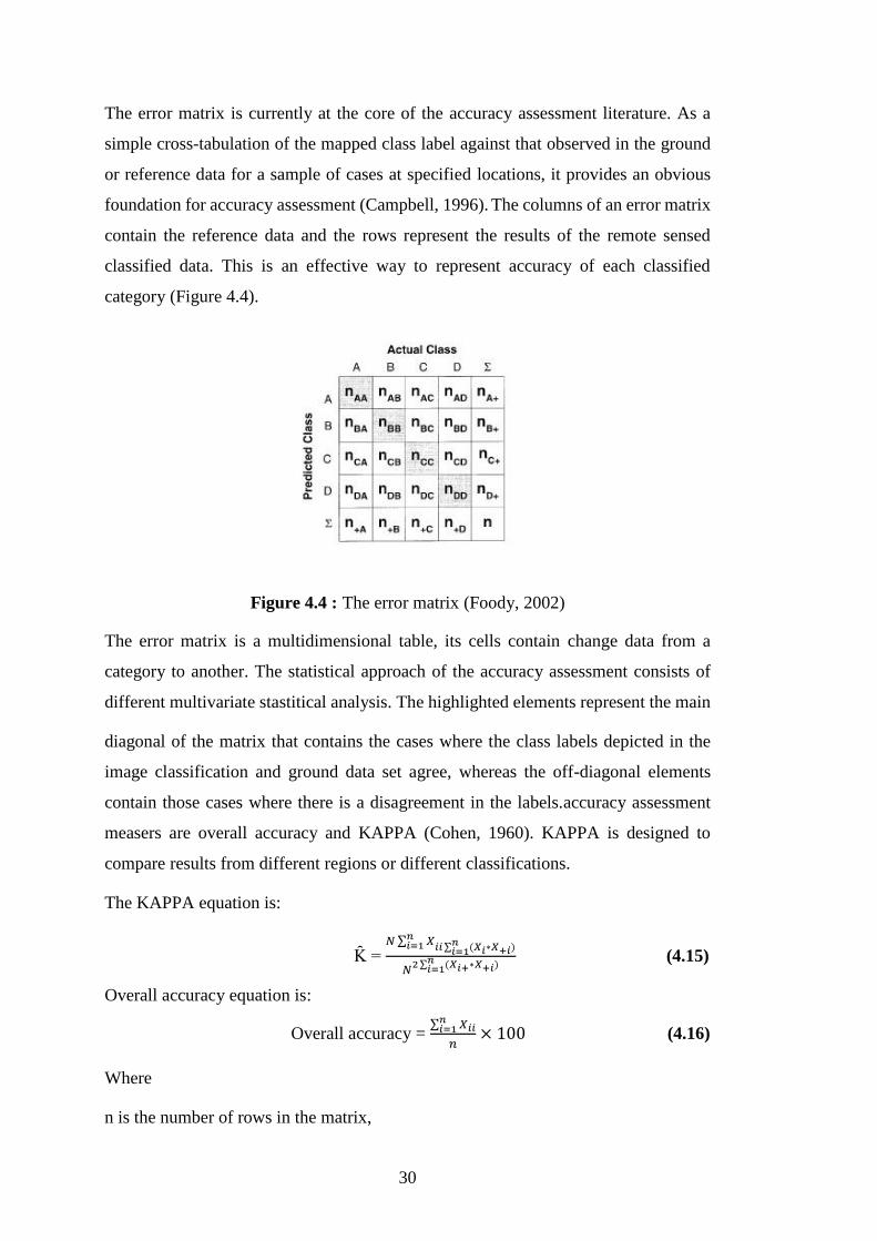
30
The error matrix is currently at the core of the accuracy assessment literature. As a
simple cross-tabulation of the mapped class label against that observed in the ground
or reference data for a sample of cases at specified locations, it provides an obvious
foundation for accuracy assessment (Campbell, 1996). The columns of an error matrix
contain the reference data and the rows represent the results of the remote sensed
classified data. This is an effective way to represent accuracy of each classified
category (Figure 4.4).
Figure 4.4 : The error matrix (Foody, 2002)
The error matrix is a multidimensional table, its cells contain change data from a
category to another. The statistical approach of the accuracy assessment consists of
different multivariate stastitical analysis. The highlighted elements represent the main
diagonal of the matrix that contains the cases where the class labels depicted in the
image classification and ground data set agree, whereas the off-diagonal elements
contain those cases where there is a disagreement in the labels.accuracy assessment
measers are overall accuracy and KAPPA (Cohen, 1960). KAPPA is designed to
compare results from different regions or different classifications.
The KAPPA equation is:
K = 𝑁 ∑ 𝑋
𝑖𝑖 ∑ (𝑋𝑖∗𝑋+𝑖)𝑛𝑖=1
𝑛𝑖=1
𝑁2 ∑ (𝑋𝑖+∗𝑋+𝑖)𝑛𝑖=1
(4.15)
Overall accuracy equation is:
Overall accuracy = ∑ 𝑋𝑖𝑖
𝑛𝑖=1
𝑛× 100 (4.16)
Where
n is the number of rows in the matrix,

31
Xii = number of observations in the row i and column I,
Xi+ = the marginal totals of row i and column I,
N = total number of observations.

32

33
STUDY AREA , DATA AND CASE STUDY
The effectiveness of remote sensing data in estimation of impervious surface and bare
land area and its accuracy was examined by using Landsat 5 TM and Landsat 8 OLI
& TIRS with 30 meters spatial resolution.
Study Area
Istanbul is located between longitudes 27° 58' and 29° 56' E and latitudes 40° 48' and
41° 36' N in northwest of turkey (Kurt, 2012). Istanbul is the biggest city of Turkey
with the population over 14.6 milion according to the Turkish Statistic Institute (2015),
showing an astonishing increase compared to 4.7 milion according to 1980 census
reports. In 1980, there were 19 districts inside Istanbul province borders; but covering
a total area of approximately 5,750 km2 , management difficulties and political reasons
led the province to to be devided into 39 districts (Kaya et al, 2014). It is surrounded
by the Black Sea in the north and the Sea of Marmara in the south. It is divided into
two parts by The Bosphorus Strait to be one in Asia and one in Europe (Balik Sanli,
2011). 25 of these districts were located in European side while 14 of them are located
in Anatolian side of Istanbul (Figure 5.1).
The land cover change occurred in Istanbul affect environment in some main fields:
Impacts on forest areas and natural grassland, on the water reservoir storage, on soil
and coastal and on the climate (Bektas Balcik, 2013). There are so many studies
concerning the impacts of land cover change in Istanbul and come with certain results.
According to a study in this region by Musaoglu et al. (2006) there is a decline of forest
areas resulted from establishment of new residential areas and illegal constructions
within forest areas.
New megaprojects such as a third bridge on the Bosphorus and a third international
airport near the northern forest region which will be located mainly on the Black Sea
coastal area of the city facing Europe will be the main threats to the natural resources
of the city, in the near future. These formerly vegetated areas will be replaced mostly

34
by artificial surfaces when the projects are completed (Bektas Balcik, 2013). A third
bridge built on the Bosphorus will obviously transform 40 % of the forest areas and
83 % of the bare and agricultural lands located in the northern part of the city into
artificial settlement areas (Ayazli, 2011).
Climate is other factor affected by land cover change. A study by Sertel and Ormeci
(2009) in the Marmara Region, which experienced significant land cover changes as a
result of rapid industrialization and population increase especially after 1980s, reveal
that anthropogenic land cover change has impacted several aspects of the regional
climate of the Marmara Region, including warming of 2 C air temperatures and the
changes in the strength and orientation of the sea breezes. Urbanization increase in
Istanbul resulted in urban heat island effect over this city (Bektas Balcik, 2013).
Climate change adversely affect animal, human, agriculture and ecosystems.
All in all, the megacity Istanbul is the economical capital of Turkey and the city has
been under the pressure of rapid and unplanned urbanization. Monitoring urban growth
and land cover change will enable the greater Istanbul metropolitan municipality for a
better management of this complex urban area (Geymen and Baz, 2008).

35
Figure 5.1 : Location of the Istanbul
Data Used
In this study, the Landsat 5 TM (20.08.2003) and Landsat 8 OLI & TIRS (06.09.2015)
satellite images with 30-meter spatial resolution were used.
5.2.1 Remote sensing satellites
A sattelite is an object that orbits around a larger object. As an example, the moon is a
satellite because it orbits around the Earth, but there are many artificial and man-made
satellites, which are launched into space and can orbit the Earth for different purposes.
Some satellites are used for taking images from other planets or the Earth’s surface
and some other satellites are used in communication. There are so many satellites with
36
different characteristics from different countries. Among all the satellites, Landsat
Thematic Mapper (TM), Landsat Multispectral Scanner System (MSS), Landsat
Enhanced Thematic Mapper Plus (ETM+), Landsat Operational Land Imager (OLI)
are freely available for mapping impervious surface and bare land area as multispectral
satellites sensor with mid-resolution. Because of the presence of short wave infrared
and long wave infrared among the bands of these satellites that are more advantageous
in Impervious surface, soil and vegetation based studies, Landsat can be categorized
as a most preferred satellite for impervious surface mapping (Xu, 2008).
5.2.2 Landsat system
Landsat satellites were first launched in 1972 with Landsat 1. For 40 years, the Landsat
satellites have provided scientists with continuous data and variety of characteristics
that has contributed to human knowledge of the water cycle, climate, ecosystems, and
the changing Earth and more.
5.2.3 Characteristics of Landsat
In the last half century deliberating of environmental change over the time was
possible for scientist using Landsat satellite. The continuous global record, medium
spatial resolution and the opening of the Landsat archives to the public in 2008 has
made this dataset one of the most prevalent in Earth system studies (Landsat 7 Science
Data Users Handbook, 2006).
Overall there are 6 Landsat satellites from beginning up to now, Landsat 1-3, Landsat
4-5, Landsat 7 and Landsat 8. Each of Landsat satellites has their own characteristics
and these are given in the next section.
5.2.3.1 Sensors and specifications
MSS (Multi Spectral Scanner), TM (Thematic Mapper), ETM (Enhanced Thematic
Mapper), ETM+ and OLI (Operational Land Imager) sensors can be named as Landsat
satellite system’s sensors.
The Landsat Multispectral Scanner (MSS) sensor was on board Landsat 1 through 5,
and acquired images of the Earth nearly continuously from July 1972 and collected
data until January 2013 when the mission of Landsat 5 was expired. MSS data was

37
acquired with a 6-bit system and has 80-meter spatial resolution while TM and ETM+
acquire data in an 8-bit system.
TM sensor has spatial resolution of 30 meter with 6 bands in NIR and SWIR portion
of spectrum while the Thermal band has 120 meter resolution. Specific technical
information of Landsat 5 TM is given in the Table 5.1 and Table 5.2.
Table 5.1 : Technical information of Landsat 5 TM.
Properties Description
Operator U.S. Geological Survey (USGS)
Launch date 1-Mar-84
Altitude 705 km (438 mi)
Life time 5 years
Orbit Sun-synchronous, Near-polar
Slope of orbit 98.2
Quantization 8 bit (256 levels)
Swath width 185 km (115 mi)
Repeat cycle 16 days
Sensors MSS (Multi Spectral Scanner) TM (Thematic Mapper)
Table 5.2 : Characteristics of Landsat 5 TM.
Band Resolution
(m)
Wavelength
(µm)
Description
1 30 (0.45-0.52) Blue
2 30 (0.52-0.60) Green
3 30 (0.63-0.69) Red
4 30 (0.76-0.90) Near Infrared
5 30 (1.55-1.75) Short wave Infrared
6 120 (10.4-12.5) Thermal Infrared
7 30 (2.08-2.35) Short wave Infrared
OLI and TIR are two sensors of Landsat 8 Earth-observation satellite as a last part of
the Landsat Data Continuity Mission. The technical information of Landsat 8 OLI &
TIRS is given in Table 5.3 and Table 5.4 (Landsat 8 (L8) data users handbook, 2016).

38
Table 5.3 : Technical information of Landsat 8 OLI & TIRS.
Properties Description
Operator U.S. Geological Survey (USGS)
Launch date 11 February 2013
Altitude 705 km (438 mi)
Life time 5-6 years
Orbit Sun-synchronous Near-polar
Slope of orbit 98.2
Quantization 12 bit(4096 levels)
Swath width 185 km (115 mi)
Repeat cycle 16 days
Sensors OLI (Operational Land Imager)
TIRS (Thermal Infrared Sensor)
Table 5.4 : Characteristics of Landsat 8 OLI & TIRS.
Band Resolution
(m)
Wavelength
(µm)
Description
1 30 (0.43-0.55) Costal aerosol
2 30 (0.45-0.51) Blue
3 30 (0.53-0.59) Green
4 30 (0.64-0.67) Red
5 30 (0.85-0.88) Near Infrared
6 60 (1.57-1.65) Short wave Infrared
7 30 (2.11-2.29) Short wave Infrared
8 15 (0.50-0.68) Panchromatic
9 30 (1.36-1.38) Cirrus
10 100(30) (10.60-11.19) Thermal Infrared
11 100(30) (11.50-12.51) Thermal Infrared
Comparing to Landsat 5 TM, Landsat 8 OLI & TIRS has several new features and
improvements (Jia et al, 2014) :
Having two OLI and TIRS sensors.
A deep blue visible channel (band 1) specifically designed for water resources
and coastal zone investigation.

39
A new infrared channel (band 9) for the detection of cirrus clouds.
The TIRS instrument collects two spectral bands for the wavelength covered
by a single band on the previous TM and ETM+ sensors.
Improvement of the spectral responses across the channels by a refined spectral
range for some bands, e.g. near-infrared (NIR) and panchromatic bands.
The data quality (signal to noise ratio) and radiometric quantization (12-bits)
of the OLI and TIRS is higher than previous Landsat instruments (8-bit for TM
and ETM+), providing significant improvement in the ability to detect changes
on the Earth’s surface.
A new Quality Assurance band is also included with each data product. This
provides information on the presence of features such as clouds, water, and
snow.
To avoid the effect of water vapour absorption NIR band is narrowed at 0.825
μm, similar to that of MODIS, and helps acquire accurate surface reflectance.
Spectral record precision is improved by enhancing the radiometric resolution
to avoid the spectral saturation comparing to previous Landsat data.
Consequently, the Landsat 8 OLI & TIRS data are anticipated to perform better for in
land cover mapping.
Data for this study is downloaded from the US Geologic survey's Earth Explorer
database (http://earthexplorer.usgs.gov) for two different dates. The dates of satellite
images used are given in the Table 5.5.
Table 5.5 : The dates of Landsat data used
LANDSAT 5 TM LANDSAT 8 OLI & TIRS
20.8.2003 06.09.2015
Data set consists of two Landsat images belonging to years 2003 and 2015 summer
cropping season. Since the study area is covering two frames of Landsat satellite (180/
31 and 180/ 32), both frames of scene are downloaded and are mosaicked and then
subsetted to Istanbul boundaries using ENVI software (5.2) to create a whole scene of
the study area (Figure 5.2).

40
(a) (b)
(c)
Figure 5.2 : Landsat 5 TM - 20/08/2003 data (a) Frame 180/ 31 (b) Frame 180/ 32
(c) Mosaic and subsetted image.
Spectral Indices
5.3.1 Built-up area indices
Various spectral built-up indices developed in numerous studies related to impervious
surface and bare land area detection and mapping, are summarized in section 4.4. In
this study, all different built-up indices represented in table 5.6 and 5.7 are examined
for all the Landsat images from years 2003 to 2015 and the result of built-up indices
are given in the Figure 5.4, Figure 5.5, Figure 5.6, Figure 5.7 and 5.8.

41
Table 5.6 : Extracted urban indices from Landsat5 TM imagery.
Abbrivation used in equations:
Band2= Green; Band3= Red; Band4= Near-Infrared; Band5= Near-Infrared; Band6= Thermal; Band7= Mid-Infrared
Name of Urban Index Abbreviation Equation Reference
Enhanced Built-Up and Bareness
Index
EBBI EBBI =
Band 5 − Band 4
10√Band 5 + Band 6
(As-syakur et al, 2012)
Index-based Built-Up Index IBI
IBI =
2Band 5
Band 5 + Band 4− [
Band 4
Band 4 + Band 3+
Band 2
Band 2 + Band 5]
2Band 5
Band 5 + Band 4+ [
Band 4
Band 4 + Band 3+
Band 2
Band 2 + Band 5]
(Xu, 2008)
Normalized Difference Build-up
Index
NDBI NDBI =
(Band 5 − Band 4)
(Band 5 + Band 4)
(Zha et al, 2003)
Urban Index NDBaI NDBaI =
Band 5 − Band 6
Band 5 + Band 6
(Kawamura et al, 1996)
Normalized Difference Bareness
Index
UI UI =
Band 7 − Band 4
Band 7 + Band 4
(Zhao and Chen, 2005)

42
Table 5.7 : Extracted urban indices from Landsat8 OLI & TIRS imagery.
Abbrivation used in equations:
Band3= Green; Band4= Red; Band5= Near Infrared; Band6= Short-wave Infrared (SWIR) 1; Band7= Short-wave Infrared (SWIR) 2; Band10=
Thermal Infrared (TIRS) 1
Name of Urban Index Abbreviation Equation Reference
Enhanced Built-Up and Bareness
Index
EBBI EBBI =
Band 6 − Band 5
10√Band 6 + Band 10
(As-syakur et al, 2012)
Index-based Built-Up Index IBI
IBI =
2Band 6
Band 6 + Band 5− [
Band 5
Band 5 + Band 4+
Band 3
Band 3 + Band 6]
2Band 6
Band 6 + Band 5+ [
Band 5
Band 5 + Band 4+
Band 3
Band 3 + Band 6]
(Xu, 2008)
Normalized Difference Build-up
Index
NDBI NDBI =
(Band 6 − Band 5)
(Band 6 + Band 5)
(Zha et al, 2003)
Urban Index NDBaI NDBaI =
Band 6 − Band 10
Band 6 + Band 10
(Kawamura et al, 1996)
Normalized Difference Bareness
Index
UI UI =
Band 7 − Band 5
Band 7 + Band 5
(Zhao and Chen, 2005)

43
Figure 5.3 : Flowchart of estimating impervious surface and bare land fraction in the
study.

44
(a)
(b)
Figure 5.4 : NDBI images of Istanbul (a) August 20, 2003 (b) September 06, 2015
As observable from NDBI images, impervious surface areas with higher NDBI values
are shown by brighter colours while the surfaces with low imperviousness are shown
by darker colours. this is a result of the minimum and maximum DNs in band 4 are
much smaller than those in band 5 for the same cover. The standardized differentiation
of these two bands will result in close to zero for forest and farmland pixels, negative
for water surfaces, but positive values for built-up pixels, enabling the latter to be
separated from the remaining covers.

45
(a)
(b)
Figure 5.5 : NDBaI images of Istanbul (a) August 20, 2003 (b) September 06, 2015
Normalized Difference Bareness Index (NDBaI) is based on significant differences of
spectral signature in the nir-infrared (band 5 Landsat5 TM) between the bare-soil and
the backgrounds. However, it shows little difference between impervious surface and
bare-soil areas in band 5. As seen in Figure 5.5 urban area is slightly dull comparing
to bare and farm lands so NDBaI is much effective in distinguishing bare-soil from
similarly impervious surface and vegetation.

46
(a)
(b)
Figure 5.6 : UI images of Istanbul (a) August 20, 2003 (b) September 06, 2015
With regard to the Figure 5.6, high amount of urban index (UI) value are represented
with lighter colours like bright grey colours, where the low UI values are shown with
dark colours that illustrates bare land and much darker UI values are classified as
vegetation.
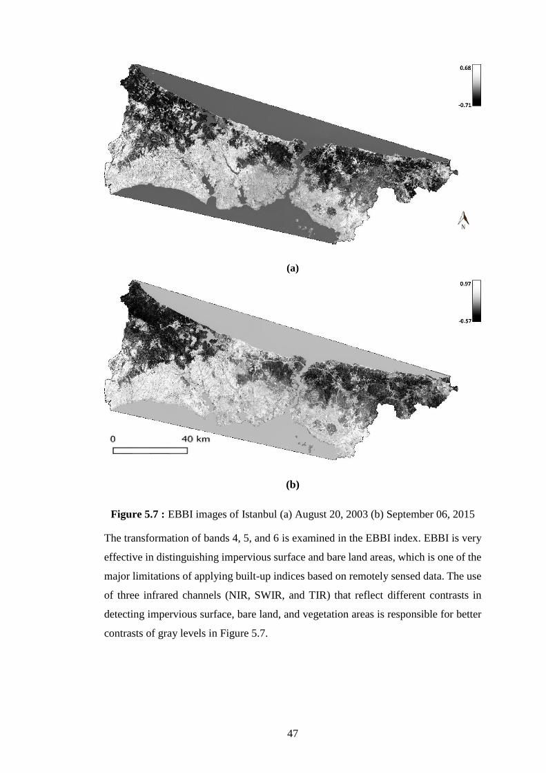
47
(a)
(b)
Figure 5.7 : EBBI images of Istanbul (a) August 20, 2003 (b) September 06, 2015
The transformation of bands 4, 5, and 6 is examined in the EBBI index. EBBI is very
effective in distinguishing impervious surface and bare land areas, which is one of the
major limitations of applying built-up indices based on remotely sensed data. The use
of three infrared channels (NIR, SWIR, and TIR) that reflect different contrasts in
detecting impervious surface, bare land, and vegetation areas is responsible for better
contrasts of gray levels in Figure 5.7.

48
(a)
(b)
Figure 5.8 : IBI image of Istanbul (a) August 20, 2003 (b) September 06, 2015
IBI is the only index that is based on other indices and it is made by using SAVI, NDBI
and MNDWI indices. IBI is proven to be one of the best urban-bare land indices used
on Landsat imagery and shows better results comparing to indices that use just two
bands .
The transformation of Landsat bands was examined in this study. This study
investigated the mapping of impervious surfaces and bare land areas by index
transformation and the results of comparing the relationship between the remote
sensing indices and the percentages of impervious surfaces and bare land areas are
detailed in this study.
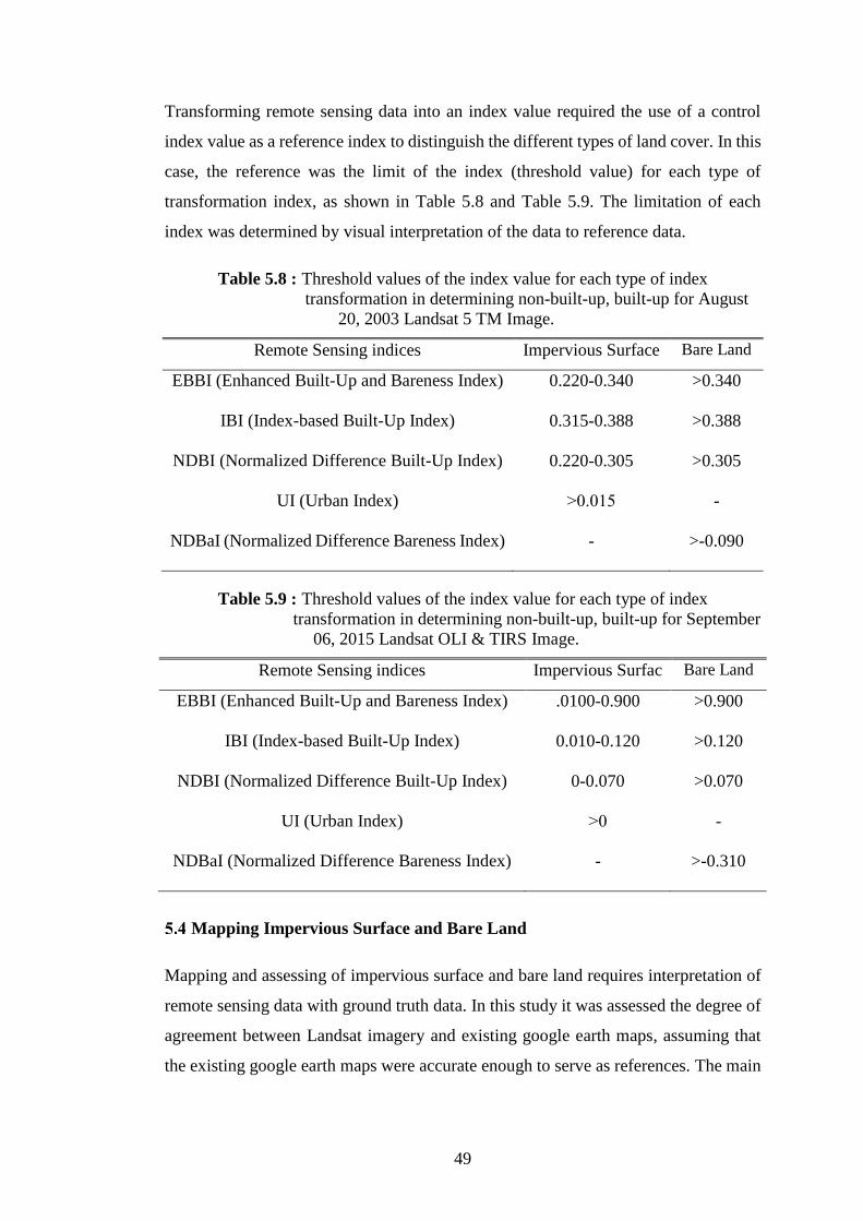
49
Transforming remote sensing data into an index value required the use of a control
index value as a reference index to distinguish the different types of land cover. In this
case, the reference was the limit of the index (threshold value) for each type of
transformation index, as shown in Table 5.8 and Table 5.9. The limitation of each
index was determined by visual interpretation of the data to reference data.
Table 5.8 : Threshold values of the index value for each type of index
transformation in determining non-built-up, built-up for August
20, 2003 Landsat 5 TM Image.
Remote Sensing indices Impervious Surface Bare Land
EBBI (Enhanced Built-Up and Bareness Index) 0.220-0.340 >0.340
IBI (Index-based Built-Up Index) 0.315-0.388 >0.388
NDBI (Normalized Difference Built-Up Index) 0.220-0.305 >0.305
UI (Urban Index) ˃0.015 -
NDBaI (Normalized Difference Bareness Index) - >-0.090
Table 5.9 : Threshold values of the index value for each type of index
transformation in determining non-built-up, built-up for September
06, 2015 Landsat OLI & TIRS Image.
Remote Sensing indices Impervious Surfac Bare Land
EBBI (Enhanced Built-Up and Bareness Index) .0100-0.900 >0.900
IBI (Index-based Built-Up Index) 0.010-0.120 >0.120
NDBI (Normalized Difference Built-Up Index) 0-0.070 >0.070
UI (Urban Index) ˃0 -
NDBaI (Normalized Difference Bareness Index) - >-0.310
Mapping Impervious Surface and Bare Land
Mapping and assessing of impervious surface and bare land requires interpretation of
remote sensing data with ground truth data. In this study it was assessed the degree of
agreement between Landsat imagery and existing google earth maps, assuming that
the existing google earth maps were accurate enough to serve as references. The main

50
reference imagery used in this study are Quick Bird images for 2003 and Wold View-
3 for 2015 images.
Then density slicing method was applied in order to classify the impervious surface
and bare land. The ranges of density slicing for each index is provided in tables 5.8
and 5.9. This ranges are obtained by comparing the classified image to the reference
data and for built-up indices the value under 0 is mostly related to vegetation, forest
and farm lands. values near 0 are likely to be water bodies. For impervious surface
detection depending on index and the data, the ranges differ and mostly it is around
0.1-0.3. Bare land area appears somehow after impervious surfaces but on some cases
it causes mixing except for NDBaI index that bare land is distinguishable even in
negative values. After classifying index derived images the impervious surface and
bare land areas were determined by each remote sensing transformation index and
represented in tables 5.10, 5.11.
Table 5.10 : Impervious surface and bare land areas of each index for August 20,
2003 Landsat 5 TM Image.
Remote Sensing indices Impervious Surface(ha) Bare Land (ha)
EBBI 121,421 63,840
IBI 117,496 38,922
NDBI 115,808 55,338
UI 48,756 -
NDBaI - 67,255
Istanbul Total Area (Except water bodies) 575,000

51
Table 5.11 : Impervious surface and bare land areas of each index for September 06,
2015 Landsat 8 OLI & TIRS Image.
Figure 5.9 shows the process of the validation of density slicing classification , class
in color blue showing bare land area and red class belongs to impervious surface area
and as seen in this image pixels are correctly classified as they are on the reference
data.
Figure 5.9 : Validation of EBBI index image of August 20, 2003 classified as
impervious surface and bare land using Quickbird August 03, 2003
image as reference.
Using the ranges given in Table 5.8 , 5.9 the impervious surface maps of Istanbul are
produced and given in Figure 5.10 and 5.11.
Remote Sensing indices Impervious Surface(ha) Bare Land (ha)
EBBI 137,406 38,432
IBI 132,155.5 26,390
NDBI 131,781 30,416.6
UI 54,682 -
NDBaI - 56,508
Istanbul Total Area (Except water
bodies)
575 ,000

52
Figure 5.10 : The spatial distribution of impervious surfaces and bare lands is shown
for each type of index/remote sensing data transformation for August
20, 2003 Landsat5 TM Image: (a) EBBI, (b) IBI, (c) NDBI, (d) UI,
(e) NDBaI

53
Figure 5.11 : The spatial distribution of impervious surfaces and bare lands is shown
for each type of index/remote sensing data transformation for September
06, 2015 Landsat8 OLI & TIRS Image: (a) EBBI, (b) IBI, (c) NDBI, (d)
UI, (e) NDBaI

54
The percentage of impervious surface area confirmed the close relationship between
the EBBI results with the percentage of actual impervious surface areas and the results
of analysis showed that the total impervious surface area obtained from the EBBI
transformation is 137,406 ha. Figure 5.10, and 5.11 show the results of this study and
following the EBBI index , IBI index results with 132,155.5 ha area in contrast to other
indices show similar pattern as EBBI Index. NDBaI index is very reliable at extracting
bare land area and almost show better results than any other index in both 2003 (67,255
ha) and 2015 (56,508 ha) images.
Accuracy Assessment
Accuracy assessment is a procedure for quantifying how good a job was done by a
classifier or how accurate out classification. In thematic mapping from remotely
sensed data, the term accuracy is used typically to express the degree of accuracy of a
map or classification. Most of the environmental features are extremely dynamic; in
most of the cases the temporal and geometric resolution of remotely sensed data cannot
cover the dynamic domain of the environmental parameters evolution (atmospheric
conditions, soil moisture, and other environmental related phenomena). Accuracy
assessment is an important part of classification. It is usually done by comparing the
classification product with some reference data that is believed to reflect the true land
cover accurately. Sources of reference data include ground truth, higher resolution
images, and maps. In this study google earth high resolution imagery was used as the
ground truth reference. (Figure 5.12)
Figure 5.12 : Missclassification of bare land as impervious surface in NDBI image
Landsat5 TM August 20, 2003 in contrast to Quickbird August 03,
2003 image.
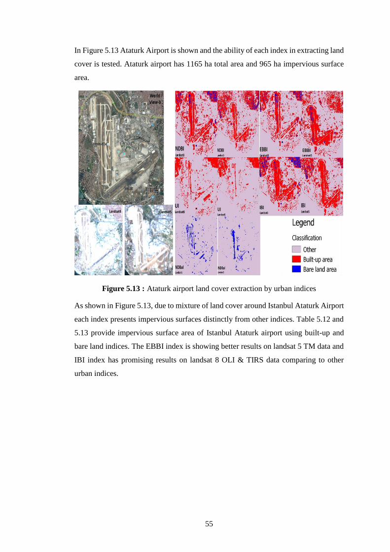
55
In Figure 5.13 Ataturk Airport is shown and the ability of each index in extracting land
cover is tested. Ataturk airport has 1165 ha total area and 965 ha impervious surface
area.
Figure 5.13 : Ataturk airport land cover extraction by urban indices
As shown in Figure 5.13, due to mixture of land cover around Istanbul Ataturk Airport
each index presents impervious surfaces distinctly from other indices. Table 5.12 and
5.13 provide impervious surface area of Istanbul Ataturk airport using built-up and
bare land indices. The EBBI index is showing better results on landsat 5 TM data and
IBI index has promising results on landsat 8 OLI & TIRS data comparing to other
urban indices.

56
Table 5.12 : Impervious surface and bare land area of farmland for each index for
August 20, 2003 Landsat5 TM Image.
Remote Sensing indices Impervious Surface(ha) Bare Land (ha)
EBBI 763 62
IBI 614 15
NDBI 387 11
UI 76 -
NDBaI - 147
Table 5.13 : Impervious surface and bare land area of farmland for each index for
September 06, 2015 Landsat8 OLI & TIRS Image.
Remote Sensing indices Impervious Surface(ha) Bare Land (ha)
EBBI 530 74
IBI 715 49
NDBI 588 67
UI 92 -
NDBaI - 173
A farmland area west of Istanbul was selected to examin the accuraccy of each index
on extarcting bare land (Figure 5.13, Table 5.16 & 5.17)
Figure 5.14 : Farmland west of Istanbul (Quickbird)

57
Table 5.14 : Impervious surface and bare land area of farmland of each index for
August 20, 2003 TM Image.
Remote Sensing indices Impervious Surface(ha) Bare Land (ha)
EBBI 3.50 202
IBI 4 185
NDBI 3.50 197
UI 168 -
NDBaI - 190
Total Area 4.50 210
Table 5.15 : Impervious surface and bare land areas of farmland of each index for
September 06, 2015 Landsat OLI & TIRS Image.
Remote Sensing indices Impervious Surface(ha) Bare Land (ha)
EBBI 6 194
IBI 26 171
NDBI 17 188
UI 69 -
NDBaI - 182
Total Area 4.50 210
Another type of urban feature is man made roads. An asphalt road by the
Buyukcavuslu in silivri district was selected to assess the capability of each index on
extracting this type of impervious surface (Figure 5.15, Table 5.16 & 5.17).
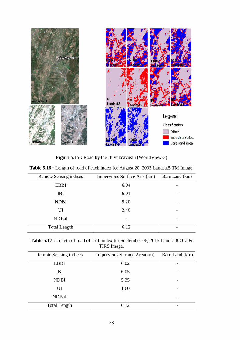
58
Figure 5.15 : Road by the Buyukcavuslu (WorldView-3)
Table 5.16 : Length of road of each index for August 20, 2003 Landsat5 TM Image.
Remote Sensing indices Impervious Surface Area(km) Bare Land (km)
EBBI 6.04 -
IBI 6.01 -
NDBI 5.20 -
UI 2.40 -
NDBaI - -
Total Length 6.12 -
Table 5.17 : Length of road of each index for September 06, 2015 Landsat8 OLI &
TIRS Image.
Remote Sensing indices Impervious Surface Area(km) Bare Land (km)
EBBI 6.02 -
IBI 6.05 -
NDBI 5.35 -
UI 1.60 -
NDBaI - -
Total Length 6.12 -

59
According to Congalton (1988) samples are selected in a order to yield too many
samples in laregr impervious surfaces and too few samples in smaller areas. As a rule
of thumb Congalton (1991) recommands at least 50 samples per class and if the area
exceeds 500 km2 then at least 75-100 samples should be chosen per class. Istanbul
having more than 5,750 km2 urban area and having just 3 classes such as impervious
surface, bare land, others; therefore random sample points was selected for each class
and to acomplish a better accuracy, google maps high resolution imagery (Quickbird
and World View-3) was used as a referance date. Others category includes forest areas,
water surfaces and vegetated areas. Result of the accurcy assessment is provided in
(Table 5.18).
Table 5.18 : Accuracy assessment result table.
Date Index Classess Overall Accuracy Kappa
2003
EBBI Impervious Surface
Bare Land
Others
89%
93%
87%
93.6%
85%
90.6%
Overall 86% 79%
IBI Impervious Surface
Bare Land
Others
84%
78%
92%
85.7%
84.8%
84%
Overall 84.6% 77%
NDBI Impervious Surface
Bare Land
Others
73%
72%
81%
80%
71%
75%
Overall 75.3% 63%
UI Impervious Surface
Bare Land
Others
90%
86%
70%
83%
77%
86.4
Overall 82% 73%
NDBaI Impervious Surface
Bare Land
Others
75%
88%
80%
87%
76.5%
89%

60
Overall 81% 71.5%
2015
EBBI Impervious Surface
Bare Land
Others
87%
83%
90%
83%
87%
90%
Overall 86% 80%
IBI Impervious Surface
Bare Land
Others
81%
89%
92%
83.5%
86%
92%
Overall 87.3% 81%
NDBI Impervious Surface
Bare Land
Others
78%
86%
79%
79%
75%
91%
Overall 81% 71.5%
UI Impervious Surface
Bare Land
Others
69%
87%
95%
92%
93.5%
72%
Overall 83.6% 75.5%
NDBaI Impervious Surface
Bare Land
Others
86%
92%
93%
95%
85%
91%
Overall 90.3% 85.5%
Classification based on Landsat 8 OLI & TIRS (September 06,2015) imagery show
better results , NDBaI index has a higher precision due to just being able to detect only
bare land area and we can observe that EBBI and IBI have the highest accuracy among
the built-up and bare land indices. Overall EBBI index has the highest accuracy results
in both data sets.

61
CONCLUSIONS AND RECOMMENDATIONS
Determination of impervious surfaces and bare lands is very important for sustainable
management and planning of urban areas such as Istanbul. Urban remote sensing
indices are generally used to extract impervious surface and bare land areas based on
spectral values with acceptable level of accuracy. High degree of homogeneity in the
land-use categories, specially in urban areas makes it difficult to achieve high accuracy
levels. Bare-soil plays an important role in the ecosystem. It could be the indicator of
urban expansion. It is very important to monitor the bare-soil areas.
In this thesis, Landsat 5 TM and Landsat 8 OLI & TIRS data obtained in two different
dates (August 20, 2003 and September 06, 2015) were used for detecting impervious
surface and bare land area in Istanbul.
Overall, five spectral indices, including the most powerful indices in the literature were
taken into consideration. Enhanced Built-up and Bareness Index (EBBI), Normalised
Difference Built-Up Index (NDBI), Index-based Built-Up Index (IBI), Urban Index
(UI), Normalised Difference Bareness Index (NDBaI) are founded as the most useful
ones.
The application of TIR channels, which exhibit high emissivity in impervious surface,
is one of the reasons that indices examining thermal band are better indices for
distinguishing between classes of land use. The high emissivity in impervious surface
areas is caused by the types of materials that are predominately found in these areas,
such as roofing and building materials. In contrast, the emissivity of bare soil is
determined by the level of soil moisture and by the mineral constituents of the soil.
Impervious surface areas exhibit higher heat conductivity than bare soil areas, resulting
in the higher emissivity and albedo values of thermal infrared waves in impervious
surfaces relative to bare soil areas.
Main conclusions which are drawn from this study, are summarized below:
Heterogeneity embedded within the nature of Istanbul makes the task of reliable and
accurate mapping of impervious surfaces and bare lands more difficult.

62
The more simultaneously collectected ground truth data with remotely sensed data are
used, the better accuracy can be observed to determine impervious surfaces and bare
lands in heterogeneous urban areas.
Most of the urban indices are generated based on homogeneous cities therefore it is
suggested to investigate the use of urban indices on heterogeneous areas in future
studies.
Besides the importance of using thermal bands in examining urban area, the EBBI
index is still a new index and it is crucial to investigate more about this index using
Landsat 8 OLI & TIRS data.
Another issue is finding proper Landsat 8 OLI & TIRS imagery without clouds in the
study area. Istanbul with a Mediterranean weather usually clouds are expected to
appear over the city. Although Landsat 8 being operational for more than three years
all over the world, hence having 16 days temporal resolution makes it hard to acquire
desired data.
One other problem is the spatial resolution of Landsat 5 TM and Landsat 8 OLI &
TIRS satellites (30 meters). The higher resolution makes the sampling easier in the
image data. In this study, the sampling of impervious surface area measurements could
be easier in the case of using higher spatial resolution.
Besides the spatial resolution, spectral resolution also plays an important role for better
interpretation of the satellite imageries. Hyperspectral sensors can be a better solution,
since they capture a large amount of narrow bands which referred to as a high spectral;
however, multispectral satellites such as Landsat 5 and 8 capture the small number of
wide bands. High spectral resolution makes it easy to distinguish between features
spectrally in the image. Since impervious surface area in the infrared and thermal
portion of electromagnetic spectrum has a strong reflectance that enables better
detection, the more these bands are available, the impervious surface area would be
detected more precisely. As a result, using the hyperspectral satellites in impervious
surface area detection could be more effective than multispectral satellites.
After comparing the results of indices, NDBaI index is considered to have promising
results for bare soil but overall EBBI index is chosen to be the more precise
transformation to make the impervious surface and bare land map of Istanbul.

63
As a conclusion, some issues named above should be considered as recommendations
for the future studies to be planned on this topic.

64

65
REFERENCES
A modern Approach to Regression with R. (2009). Sheather, S., Springer Science &
Business Media.
Arnold, C. L. Jr., and Gibbons, C. J. (1996). Impervious surface coverage: The
emergence of a key environmental indicator. Journal of the American
Planning Association, 62, 243–258.
As-Syakur, A. R., Adnyana, I., Arthana, I. W., and Nuarsa, I. W. (2012). Enhanced
Built-Up and Bareness Index (EBBI) for mapping built-up and bare
land in an urban area. Remote Sensing, 4(10), 2957-2970.
Ayazli, I. E. (2011). Simulation model of urban sprawl driven by transportation
networks: 3rd Bosphorus bridge example. (Ph.D. Thesis). Yildiz
Technical University, Istanbul.
Balçik, F. B. (2013). Determining the impact of urban components on land surface
temperature of Istanbul by using remote sensing indices. Environmental
monitoring and assessment, 186(2), 859-872.
Bellard, C., Bertelsmeier, C., Leadley, P., Thuiller, W., and Courchamp, F. (2012). Impacts of climate change on the future of biodiversity. Ecology
letters, 15(4), 365-377.
Braun, M., & Herold, M. (2004). Mapping imperviousness using NDVI and linear
spectral unmixing of ASTER data in the Cologne-Bonn region
(Germany). Proceedings of the SPIE 10th international symposium on
remote sensing, Barcelona, Spain, 8–12 Sept 2003.
Brun, S. E., and Band, L. E. (2000). Simulating runoff behavior in an urbanizing
watershed. Computers, Environment and Urban Systems, 24, 5–22.
Burak, S., Doǧan, E. and Gazioǧlu, C. (2004). Impact of urbanization and tourism
on coastal environment. Ocean and Coastal Management, 47, pp.515–
527.
Borges, J. S. (2008). Bayesian hyperspectral image segmentation with discriminative
class learning. University of Porto, Porto, Portuguese.
Chen, X-L., Zhao, H-M., Li, P-X., and Yin, Z-Y. ( 2006). Remote sensing image-
based analysis of the relationship between urban heat island and land
use/cover changes. Remote Sensing of Environment, 104, 133–146.

66
Chen, J., Zhu, X., Vogelmann, J. E., Gao, F., and Jin, S. (2011). A simple and
effective method for filling gaps in Landsat ETM+ SLC-off images.
Remote Sensing of Environment, 115,4. p: 1053-64.
Coban, H.O., Koc, A. and Eker, M. (2010). Investigation on changes in complex
vegetation coverage using multi-temporal landsat data of Western
Black sea region - A case study. Journal of Environmental Biology, 31,
pp.169–178.
Congalton, R. (1988) A comparison of sampling schemes used in generating error
matrices for assessing the accuracy of maps generated from remotely
sensed data. Photogrammetric Engineering and Remote Sensing,
54(5):593–600.
Congalton, R. (1991) A Review of Assessing the Accuracy of Classifications of
Remotely Sensed Data. Remote Sensing of Environment, 37:35–46.
Elvidge, C. D., Tuttle, B. T., Sutton, P. C., Baugh, K. E., Howard, A. T., Milesi,
C., and Nemani, R. (2007). Global distribution and density of
constructed impervious surfaces. Sensors, 7(9), 1962-1979.
Encyclopedia of Geographic Information Science. (2008). Karen, K. K.
Encyclopedia of geographic information science. (2008). Kemp, K., Sage.
ERDAS, Inc. (1999). ERDAS Field Guide, 5th edition, ERDAS Inc., Atlanta, GA.
ERDAS, Inc. (2014). Fundamentals of ERDAS Imagine, Atlanta, GA.
Flanagan, M. (2001). Subpixel Impervious Surface Mapping. Proceedings of the
ASPRS Annual Conference, , St.Louis, Missouri, USA, April 23-27,
2001.
Foody, G. M. (2002). Status of land cover classification accuracy assessment. Remote
sensing of environment, 80(1), 185-201
Fundamentals of remote sensing and airphoto interpretation. (1992). Avery, T. E.,
and Berlin, G. L.
Geymen, A. and Baz, I. (2008). Monitoring urban growth and detecting land-cover
changes on the Istanbul metropolitan area. Environmental monitoring
and assessment, 136(1-3), pp.449–459.
Goksel, C., Musaoglu, N., Gurel, M., Ulugtekin, N., Tanik, A., and Seker, D. Z.
(2006). Determination of land-use change in an urbanized district of
Istanbul via remote sensing analysis. Fresenius Environmental Bulletin,
15(8a), 798–805.
Hasanlou M., and Mostofi N. (2015). Investigating Urban Heat Island Estimation
and Relation between Various Land Cover Indices in Tehran City
Using Landsat 8 Imagery. 1st International Electronic Conference on
Remote Sensing, 22 June-05 July 2015.

67
Harris, S., Veraverbeke, S., and Hook, S. (2011). Evaluating spectral indices for
assessing fire severity in chaparral ecosystems (Southern California)
using MODIS/ASTER (MASTER) airborne simulator data. Remote
sensing, 3(11), 2403-2419.
Hurd, J. D., and Civco, D. L. (2004). Temporal characterization of impervious
surfaces for the State of Connecticut. ASPRS Annual Conference
Proceedings, Denver, Colorado, May 2004 (Unpaginated CD-ROM).
Introduction to the physics and techniques of remote sensing (Vol. 28). (2006).
Elachi, C., and Van Zyl, J. J., John Wiley & Sons.
Jia, K., Wei, X., Gu, X., Yao, Y., Xie, X., and Li, B. (2014). Land cover classification
using Landsat 8 operational land imager data in Beijing, China.
Geocarto International, 29(8), 941-951.
Fundamentals of remote sensing. (2005). Joseph, G., Universities Press.
Kaya, S. and Curran, P.J. (2006). Monitoring urban growth on the European side of
the Istanbul metropolitan area: A case study. International Journal of
Applied Earth Observation and Geoinformation, 8(1), pp.18–25.
Kaya, S., Osgouei, P. E., Alganci, U., Seker, D. Z. and Gazioglu, C. (2015).
Evaluation of Vegetation Density Changes in Suburban Area: A Case
Study of Istanbul Metropolitan Area. ACRS 2015: The 36 th Asian
Conference on Remote Sensing “Fostering Resilient Growth in Asia”,
Quezon City, Metro Manila, Philippines, 19-23 October 2015, pp.1-2
.Kurt, S. (2012). Land Use Changes in Istanbul’s Marmara Sea Coastal Regions
Between 1987 and 2007. Middle-East Journal of Scientific Research,
11 (11): 1584-1590, 2012
Landsat 7 Science Data USers Handbook. http://ltpwww.gsfc.nasa.gov/IAS/handbook/handbook_toc.html. date
retrieved 10.05.2016.
Landsat, U. S. G. S. 8 (L8). (2016) Data Users Handbook Version 1.0.
Masek, J.G., F.E. Lindsay and Goward, (2000). Dynamics of urban growth in the
Washington DC metropolitan area, 1973-1996, from Landsat
observations. International Journal of Remote Sensing, 21(18):
pg.3473-3486.
Merriam-Webster's Collegiate Dictionary Thesaurus : Electronic Edition, Version
1. (1994). Merriam Webster.
Musaoglu, N., Tanik, A., and Kocabas, V. (2005). Identification of Land-Cover
Changes Through Image Processing and Associated Impacts on Water
Reservoir Conditions. Environmental Management, Vol. 35, No. 2, pp.
220–230

68
Musaoglu, N., Gurel, M., Ulugtekin, N., Tanik, A., and Seker, D. Z. (2006). Use of
remotely sensed data for analysis of land-use change in a highly
urbanized district of mega city, Istanbul. Journal of Environmental
Science and Health, Part A, 41(9), 2057-2069.
Mundhe, N. N., and Jaybhaye, R. G. (2014). Impact of urbanization on land use/land
covers change using Geo-spatial techniques. International journal of
geomatics and geosciences, Volume 5, No 1, 2014
Principles of remote sensing. Longman Inc. (1985). Curran, P. J.
Remote sensing and image interpretation. (2014). Lillesand, T., Kiefer, R. W., and
Chipman, J., John Wiley & Sons.
Remote Sensing of the Environment: An Earth Resource Perspective (2nd Edition). (2009). Jensen, J. R., Pearson Education India.
Remote sensing: models and methods for image processing. (2006). Schowengerdt,
R. A., Academic press.
Rikimaru, A., and Miyatake, S. (1997). Development of Forest Canopy Density
Mapping and Monitoring Model using Indices of Vegetation, Bare soil
and Shadow. In Proceeding of the 18th Asian Conference on Remote
Sensing (ACRS) 1997, Kuala Lumpur, Malaysia, 20–25; p. 3.
Sanli, F. B., Balcik, F. B., and Goksel, C. (2008). Defining temporal spatial patterns
of mega city Istanbul to see the impacts of increasing population.
Environmental monitoring and assessment, 146(1-3), 267-275.
Schueler, T. R. (1994). The Importance of Imperviousness. Watershed Protection
Techniques, vol. 1, no. 3.
Singh, R. P., and Sirohi, A. (1995). Spectral Reflectance Properties of Different
Types of Built-up Surfaces. Journal of Aerospace Engineering, Vol. 8,
No. 1, pp. 25-31
Sleavin, W. J. (1999). Measuring Impervious Surfaces in Connecticut Using
Planimetric GIS Data. (Thesis). Department of Natural Resource
Management and Engineering, University of Connecticut, Storrs, CT.
Sleavin, W. J., Civco, D. L., Prisloe, S., and Giannotti, L. (2000). Measuring
impervious surfaces for non-point source pollution modeling. In
Proceedings of the ASPRS 2000 Annual Convention. (pp. 22-26).
Song, D. X., Huang, C., Sexton, J. O., Channan, S., Feng, M., and Townshend, J.
R. (2015). Use of Landsat and Corona data for mapping forest cover
change from the mid-1960s to 2000s: Case studies from the Eastern
United States and Central Brazil. ISPRS Journal of Photogrammetry
and Remote Sensing, 103, 81-92.

69
Stankowski, S. J. (1972). Population Density as an Indirect Indicator of Urban and
Suburban Land-Surface Modifications. U.S. Geological Survey
Professional Paper, 800-B.
Turner, B., Skole, D., Sanderson, S., Fischer, G., Fresco, L., and Leemans, R.
(1995). Land-use and land-cover change In International Geosphere-
Biosphere Programme (Report No. 35). Stockholm.
Van Niel, T. G. (1995). Classification of vegetation and analysis of its recent trends
at Camp Williams, Utah using remote sensing and geographic
information system techniques. Utah State University. Department of
Watershed Science.
Url-1 <http://www.gisresources.com/an-insight-to-ndvi_2/>, date retrieved
10.04.2016.
Url-2 <http://www.mdcoastalbays.org/bayissues-stormwater-management>, date
retrieved 18.05.2016.
Url-3 <http://www.shariqa.com/waves%20around%20us.htm>, date retrieved
15.04.2016.
Url-4 <http://en.wikipedia.org/wiki/Remote_sensing>, date retrieved 15.04.2016.
Url-5 < http://www.turkstat.gov.tr>, date retrieved 26.05.2016
Weng, Q. (2008). Remote Sensing of Impervious Surfaces: An Overview. In Remote
Sensing of Impervious Surfaces.
Weng, Q. (2012). Remote sensing of impervious surfaces in the urban areas:
Requirements, methods, and trends. Remote Sensing of Environment,
117, 34-49.
Xu, H. (2007). Extraction of Urban Built-up Land Features from Landsat Imagery
Using a Thematic-oriented Index Combination Technique.
Photogrammetric Engineering Remote Sensing, Vol. 73, No. 12, pp.
1381-1391
Xu, H. (2008). A new index for delineating built-up land features in satellite imagery.
Int. J. Remote Sens, 2008, 29, 4269–4276.
Yitong, J., Fu, P., and Weng, Q. (2015). Assessing the Impacts of Urbanization-
Associated Land Use/Cover Change on Land Surface Temperature and
Surface Moisture: A Case Study in the Midwestern United States.
Remote Sens, 2015, 7, 4880-4898; doi:10.3390/rs70404880
Yuan, F., Sawaya, K. E., Loeffelholz, B. C., and Bauer, M. E. (2005). Land cover
classification and change analysis of the Twin Cities (Minnesota)
Metropolitan Area by multitemporal Landsat remote sensing. Remote
sensing of Environment, 98(2), 317-328.

70
Zha, Y., Gao, J., and Ni, S. (2003). Use of normalized difference built-up index in
automatically mapping urban areas from TM imagery. Int. J. Remote
Sens, 24, 583–594.
Zhao, H. M. and Chen, X. L. (2005). Use of Normalized Difference Bareness Index
in Quickly Mapping Bare Areas from TM/ETM+. In Proceedings of
2005 IEEE International Geoscience and Remote Sensing Symposium,
Seoul, Korea, 25–29; Volume 3, pp. 1666-1668.

71
CURRICULUM VITAE
Name Surname : Kaveh KHORSHID
Place and Date of Birth : Iran , 01.09.1984
E-Mail : [email protected]
B.Sc. : 2011, Urmia University, Civil Engineering Department