Embed Size (px)
Citation preview
Stamatia DimopoulouEnergy Management of a Hybrid EnergyStorage System in a single-family Houseincluding E-Car Mobility
SSE-Dissertation 17
SoftwareSystemsEngineering
Department of InformaticsChair of Prof. Dr. Andreas Rausch

Energy Management of a Hybrid EnergyStorage System in a single-family House
including E-Car Mobility
Doctoral Thesis(Dissertation)
to be awarded the degree ofDoctor of Engineering
(Dr.Ing.)
submitted by
Stamatia Dimopouloufrom Athens, Greece
approved by the Department of Informatics,Clausthal University of Technology
2018

Dissertation Clausthal, SSE-Dissertation 17, 2018
Chairperson of the Board of ExaminersProf. Dr. Sven Hartmann
Chief ReviewerProf. Dr. Andreas Rausch
2. ReviewerProf. Dr. rer. nat. habil. Ekkehard Boggasch
3. ReviewerProf. Dr.-Ing. Joachim Landrath
Date of oral examination: November 19, 2018

iii
To my parents

iv
v
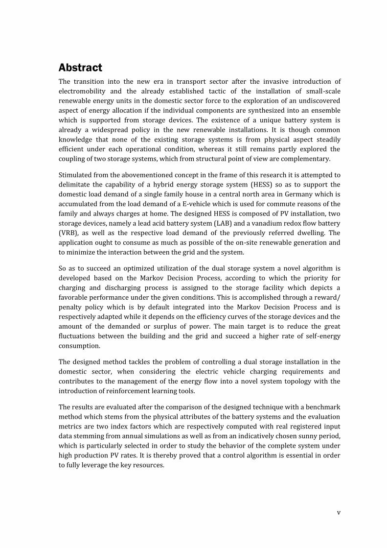
Abstract The transition into the new era in transport sector after the invasive introduction of
electromobility and the already established tactic of the installation of small-scale
renewable energy units in the domestic sector force to the exploration of an undiscovered
aspect of energy allocation if the individual components are synthesized into an ensemble
which is supported from storage devices. The existence of a unique battery system is
already a widespread policy in the new renewable installations. It is though common
knowledge that none of the existing storage systems is from physical aspect steadily
efficient under each operational condition, whereas it still remains partly explored the
coupling of two storage systems, which from structural point of view are complementary.
Stimulated from the abovementioned concept in the frame of this research it is attempted to
delimitate the capability of a hybrid energy storage system (HESS) so as to support the
domestic load demand of a single family house in a central north area in Germany which is
accumulated from the load demand of a E-vehicle which is used for commute reasons of the
family and always charges at home. The designed HESS is composed of PV installation, two
storage devices, namely a lead acid battery system (LAB) and a vanadium redox flow battery
(VRB), as well as the respective load demand of the previously referred dwelling. The
application ought to consume as much as possible of the on-site renewable generation and
to minimize the interaction between the grid and the system.
So as to succeed an optimized utilization of the dual storage system a novel algorithm is
developed based on the Markov Decision Process, according to which the priority for
charging and discharging process is assigned to the storage facility which depicts a
favorable performance under the given conditions. This is accomplished through a reward/
penalty policy which is by default integrated into the Markov Decision Process and is
respectively adapted while it depends on the efficiency curves of the storage devices and the
amount of the demanded or surplus of power. The main target is to reduce the great
fluctuations between the building and the grid and succeed a higher rate of self-energy
consumption.
The designed method tackles the problem of controlling a dual storage installation in the
domestic sector, when considering the electric vehicle charging requirements and
contributes to the management of the energy flow into a novel system topology with the
introduction of reinforcement learning tools.
The results are evaluated after the comparison of the designed technique with a benchmark
method which stems from the physical attributes of the battery systems and the evaluation
metrics are two index factors which are respectively computed with real registered input
data stemming from annual simulations as well as from an indicatively chosen sunny period,
which is particularly selected in order to study the behavior of the complete system under
high production PV rates. It is thereby proved that a control algorithm is essential in order
to fully leverage the key resources.

vi

vii
Acknowledgement
This thesis was conducted in the frame of the Cooperative Promotion Program
Electromobility (Kooperatives Promotionsprogramm Elektromobilität) which in terms of a
schloraship aided financially for 3 years the current research, in cooperation and
collaboration of the Institute for Applied Software Systems Engineering, TU Clausthal,
Clausthal-Zellerfeld, Germany and the Laboratory of Electrical Engineering and Renewable
Energy Systems, Faculty of Supply Engineering, Ostfalia University of Applied Sciences,
Wolfenbüttel, Germany. Moreover, I would like to express my gratitude to the Rud. Otto
Meyer-Umwelt-Stiftung which financially supported further my PhD study during the last
months.
For the fulfillment of this thesis several people have contributed with their generous
providing of input, comments and remarks. First of all I would like to thank my supervisors,
Prof. Dr. Andreas Rausch and Prof. Ekkehard Boggasch for their continuous support during
the individual steps of the research, their dedicate reading of the study as well as for their
constructive comments after numerous brainstorming meetings and discussions.
In addition special thanks are due to the entire research team of the Laboratory of Electrical
Engineering and Renewable Energy Systems of the Ostfalia University who steadily
supported me and in particular to Dr. Lars Baumann and Patrick Kügler whom models of
their studies and work were integrated in the current study, and Alice Oppermann whose
daily and constant technical know-how but also psychological encouragement helped me go
through this journey.
Last but not least, I would like to thank my family. My brother Dimitri, for his continuous
support in every occasion that has arisen, my beloved husband George, since without his
support, patience and inspiration in all terms I would not have completed this thesis, as well
as my two adorable children, Anastasia and Alexandro, for their understanding for all the
moments which I could dedicate playing with them but instead I had to sacrifice in order to
keep writing and finalizing my PhD study.

viii
ix
Table of Contents Abstract ................................................................................................................................................ v
Acknowledgement ........................................................................................................................... vii
List of Figures.................................................................................................................................. xiii
List of Tables ..................................................................................................................................... xv
Abbreviations .................................................................................................................................xvii
1 Introduction ................................................................................................................................ 1
1.1 Motivation ......................................................................................................................................................... 1
1.2 Aim & Objectives ........................................................................................................................................... 3
1.3 Methodology .................................................................................................................................................... 4
1.4 Thesis Layout .................................................................................................................................................. 5
2 System Fundamentals & Experimental Setting ................................................................. 7
2.1 Energy Park of the Ostfalia University ............................................................................................... 7
2.2 Solar Photovoltaic Systems ...................................................................................................................... 9
2.2.1 State of the Art of Photovoltaic .................................................................................................... 9
2.2.2 Description of the on-site Phovoltaic (PV) installation................................................ 11
2.2.3 Modeling of Photovoltaic Systems .......................................................................................... 13
2.3 Stationary Storage Systems .................................................................................................................. 14
2.3.1 State of the Art of Electrochemical Storage Systems ..................................................... 15
2.3.2 Lead Acid Battery ............................................................................................................................. 16
2.3.2.1 Description of the on-site Lead Acid Battery ................................................... 18
2.3.2.2 Modeling of Lead Acid Battery System ............................................................ 20
2.3.3 Vanadium Redox Flow Battery ................................................................................................. 21
2.3.3.1 Description of the on-site Vanadium Redox Flow Battery ............................... 22
2.3.3.2 Modeling of the Vanadium Redox Flow Battery System .................................. 23
2.4 Residential Load Demand including E-Vehicle Charging ...................................................... 24
2.4.1 Residential Load Demand ............................................................................................................ 24
2.4.1.1 Modeling of the Load Demand of a Residence ................................................ 25
2.4.2 E-Vehicle Load Demand................................................................................................................ 26
2.4.2.1 Description of the On-Site E-Vehicle & Charging Station ................................. 27
2.4.2.2 Modeling of E-Vehicle Load Demand .............................................................. 28
3 Hybrid Energy Storage System ............................................................................................ 29
3.1 Introduction to Hybrid Energy Storage System (HESS)......................................................... 29
3.2 Description of In-Situ HESS .................................................................................................................. 30
x
3.3 Problem Description & Scope of this Work ..................................................................................31
3.3.1 Overall Problem ................................................................................................................................32
3.3.2 Examined Approach ........................................................................................................................32
3.3.3 State of the Art of Control Management Concepts ..........................................................33
3.3.4 Beyond the State of the Art .........................................................................................................35
3.3.5 Evaluation Criteria...........................................................................................................................37
3.4 Research Questions ...................................................................................................................................38
3.5 Limitations of Scope & Challenges.....................................................................................................39
4 Hybrid Energy Storage System Modeling ......................................................................... 41
4.1 Photovoltaic Model ....................................................................................................................................41
4.1.1 Decomposition Models ..................................................................................................................45
Isotropic Sky Model ............................................................................................ 45 A.
Klucher Model .................................................................................................... 45 B.
Perez Model ....................................................................................................... 46 C.
4.2 Lead Acid Battery Model.........................................................................................................................48
4.3 Vanadium Redox Flow Battery Model .............................................................................................54
4.4 Residential Load Demand Model........................................................................................................58
4.5 Electric-Vehicle Load Demand Model ..............................................................................................59
4.6 Grid Model ......................................................................................................................................................61
5 Energy Management System ................................................................................................ 63
5.1 Introduction to Markov Decision Process .....................................................................................63
5.2 Designed Markov Decision Process Controlling .........................................................................66
5.2.1 Battery Efficiencies and Previous Work ...............................................................................66
5.2.2 Markov Process of the Examined System ............................................................................67
5.2.3 Implementation .................................................................................................................................73
5.3 Naive Approach-Benchmark Method ...............................................................................................76
5.4 Overall Model - Interactions of the Models ...................................................................................77
6 Simulation Results & Discussion ........................................................................................ 79
6.1 Simulation Results with one Storage System ...............................................................................79
Outcomes with Lead Acid Battery ....................................................................... 81 A.
Outcomes with Vanadium Redox Flow Battery ................................................... 83 B.
6.2 Simulation Results with Two Storage Systems ...........................................................................84
Outcomes from Naive Approach ......................................................................... 84 A.
Outcomes from Markov Decision Process Controlling ......................................... 86 B.
6.3 Evaluation & Discussion of Results ...................................................................................................89

xi
7 Conclusions & Perspective .................................................................................................... 95
References ......................................................................................................................................... 99
A. Appendix .................................................................................................................................. A-1
PV Model .......................................................................................................... A-1 A.
Lead Acid Battery Model ................................................................................... A-1 B.
Vanadium Redox Flow Battery Model ................................................................ A-2 C.
Grid Model ........................................................................................................ A-4 D.

xii
xiii
List of Figures Figure 1-1: Followed Methodology .......................................................................................................................... 5
Figure 2-1: Graphical Representation of the Energy Park [18] ................................................................. 8
Figure 2-2: PV Data in Germany during the last 15 years [25] .................................................................. 9
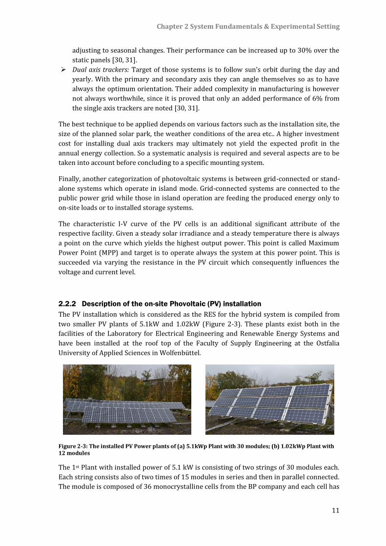
Figure 2-3: The installed PV Power plants of (a) 5.1kWp Plant with 30 modules; (b)
1.02kWp Plant with 12 modules ............................................................................................................................ 11
Figure 2-4: Efficiency Curve of the Sunny Boy 2000 [32] ......................................................................... 12
Figure 2-5: Efficiency Curve of the Sunny Boy 1200 [33] ......................................................................... 13
Figure 2-6: Model for PV cells with a single-diode ....................................................................................... 14
Figure 2-7: Storage Systems Classification according to type of stored energy [46].................. 15
Figure 2-8: Lead Acid Battery with Sunny Backup System 5000 .......................................................... 19
Figure 2-9: Charge Control of the Sunny Backup 5000 [61] .................................................................... 19
Figure 2-10: Equivalent Circuit Model for Battery........................................................................................ 20
Figure 2-11: Graphical Representation of the Equivalent Circuit Models ........................................ 21
Figure 2-12: Vanadium Redox Flow Battery coupled at the Energy Park at the Ostfalia
University ........................................................................................................................................................................... 22
Figure 2-13: Schematic illustration of the installed Vanadium System with its auxiliary
components [18] ............................................................................................................................................................. 23
Figure 2-14: Equivalent Electrical Model of the Vanadium Redox Flow Battery [18] ............... 24
Figure 2-15: Yearly Electricity Consumption per Household with & without Heating [78] ... 25
Figure 2-16: EV Peugeot iOn with Charging Station .................................................................................... 27
Figure 3-1: Hybrid System Synthesis ................................................................................................................... 30
Figure 3-2: Block Diagram of the installed facilities depicting the energy & information flow
.................................................................................................................................................................................................. 33
Figure 4-1: Global Radiation Components ........................................................................................................ 42
Figure 4-2: Solar incidence angle on a PV panel ............................................................................................ 44
Figure 4-3: Flow Chart Diagram of the Lead Acid Battery Model ......................................................... 49
Figure 4-4: Efficiency of the Inverter Sunny Backup 5000 ....................................................................... 51
Figure 4-5: Open-Circuit Voltage as function of State of Charge ........................................................... 52
Figure 4-6: Internal Charge & Discharge Resistance as function of State of Charge ................... 53
Figure 4-7: Graphical Illustration of the Voltage, Current & SOC during Charge .......................... 53
Figure 4-8: The installed PV Power plants of (a) 5.1kWp Plant with 30 modules; (b)
1.02kWp Plant with 12 modules ............................................................................................................................ 54
Figure 4-9: Validation Test Results [18] ............................................................................................................. 58
Figure 4-10: Typical Reference Load Profile for a Summer Workday (SWX) ................................. 59
xiv
Figure 4-11: Electric Load Demand of the 14.4 kWh Lithium iOn Battery of the Peugeot iOn
after a Real Driving Combined Cycle of 60km .................................................................................................60
Figure 4-12: Cumulative Daily Load for a Summer Workday (SWX)...................................................60
Figure 5-1: A graphical illustration of a MDP model ....................................................................................64
Figure 5-2: Efficiency Grades of Storage Systems ..........................................................................................66
Figure 5-3: Graphical Illustration of the 𝑆𝑂𝐶𝐿𝐴𝐵𝑡 transition ....................................................................71
Figure 5-4: Implementation Architecture ..........................................................................................................75
Figure 5-5: Schematic Illustration of the Applied Strategy .......................................................................76
Figure 5-6: Simulink Model Layout [133-135] ................................................................................................78
Figure 6-1: A graphical illustration of the Annual Load Profile ..............................................................80
Figure 6-2: A graphical illustration of the annual PV production .........................................................80
Figure 6-3: A graphical illustration of load demand and the PV production from 3rd till 11th of
June 2013 ............................................................................................................................................................................81
Figure 6-4: Annual Percentage Breakdown of the On-Site Power Generation (Naive Policy)
..................................................................................................................................................................................................86
Figure 6-5: Annual Percentage Breakdown of the On-Site Power Generation (Markov Policy)
..................................................................................................................................................................................................88
Figure 6-6: Monthly Illustration of Calculated Supply Cover Factor ...................................................90
Figure 6-7: Monthly Illustration of Calculated Grid Interaction Index ...............................................90
Figure 6-8: Annual Rate of Self-Energy Consumption for 4 Case Studies .........................................92
Figure 6-9: Rate of Self-Energy Consumption for 4 Case Studies during a Sunny Period ........92
Figure 6-10: Monthly Energy Allocation of the On-Site Generation (Naive Policy) .....................93
Figure 6-11: Monthly Energy Allocation of the On-Site Generation (Markov Policy).................93
Figure A-1: A graphical illustration of the PV Model [41, 111, 112] ..................................................A-1
Figure A-2: DC-Power Calculation according to Perpiñan et al. [112] ..............................................A-1
Figure B-1: A graphical illustration of the LAB Model [58, 125] ..........................................................A-1
Figure B-2: A graphical illustration of the Voltage Drop on the Overall Internal Resistance
[58] .......................................................................................................................................................................................A-2
Figure B-3: SOC-Calculation for the LAB Model [58] .................................................................................A-2
Figure C-1: A graphical illustration of the VRB Model [18] ....................................................................A-2
Figure C-2: A graphical illustration of the VRB System Control [18] .................................................A-3
Figure C-3: A graphical illustration of the Operational Control of the VRB Model [18]...........A-3
Figure C-4: Efficiency Stack Current Calculation [18] ...............................................................................A-4
Figure C-5: SOC-Calculation for the VRB Model [18] .................................................................................A-4
Figure D-1: A graphical illustration of the Grid Model ..............................................................................A-4
xv
List of Tables Table 2-1: Manufacturer’s Specifications of installed panels .................................................................. 12
Table 2-2: Tilt Angle per Month of 1.02kWp PV Plant ................................................................................ 13
Table 2-3: Characteristics of Battery Systems ................................................................................................. 16
Table 4-1: Constants for the determination of 𝐹1 and 𝐹2 as a function of ε ..................................... 47
Table 4-2: Total Error of Output Energy in 2013 .......................................................................................... 48
Table 4-3: Calculated coefficients for Req [18] ................................................................................................. 56
Table 4-4: Estimated Power Consumption of the Auxiliary Systems [18] ....................................... 57
Table 4-5: Typical-day categories .......................................................................................................................... 59
Table 6-1: Simulation Energy Results (with LAB) ......................................................................................... 82
Table 6-2: Simulation Energy Results (with VRB) ........................................................................................ 83
Table 6-3: Annual Simulation Energy Results (Naive Policy) ................................................................. 85
Table 6-4: Simulation Energy Results for Sunny Period (Naive Policy) ............................................ 85
Table 6-5: Annual Simulation Energy Results (Markov Policy) ............................................................. 87
Table 6-6: Simulation Energy Results for Sunny Period (Markov Policy) ........................................ 87
Table 6-7: Evaluation Criteria (2013) ................................................................................................................. 89
Table 6-8: Evaluation Criteria (Sunny Period) ................................................................................................ 89
Table 6-9: Overall System Energy Efficiency Ratio ....................................................................................... 91

xvi

xvii
Abbreviations
AGM Absorbed Glass Mat
BOP Balance-Of-Plant
CHP Combined Heat and Power
CO2 Carbon Dioxide
DWD Deutscher Wetterdienst (German Meteorological Service)
EER Energy Efficiency Ratio
HESS Hybrid Energy Storage System
LAB Solar Lead Acid Battery System
LON Local Operating Network
MBE Mean Bias Error
MDP Markov Decision Process
MPP Maximum Power Point
OPC Open Platform Communications
PDF Probability Density Function
PLC Programmable Logic Controller
PV Photovoltaic
RES Renewable Energy Source
RTU Remote Terminal Unit
UPS Uninterruptible Power Supply
VDEW Verband der Elektrizitätswirtschaft
VRB Vanadium Redox Flow Battery
VRLA Valve Regulated Lead Acid Battery

xviii
Chapter 1 Introduction
1
1 Introduction The increase of greenhouse gas emissions during the last decades, the challenge of global
warming which threatens the orderly life on Earth and the Fukushima nuclear disaster have
set the adoption of radical measures in the primary energy production as pivotal. The First
and Second European Climate Change Programme, launched in 2000 and 2005 respectively
and referring to all the EU Members [1], the Chinese Renewable Energy Law passed in 2005
and amended in 2009 [2], the Energy Transition (Energiewende) policy which was
introduced in 2010 [3] in Germany are only some paradigms of the extended effort of the
governmental and legislative organs to promote globally renewable energy sources and
energy efficiency in order to substitute fossil fuels and nuclear energy in the overall energy
mix.
The building sector has globally the highest ratio in energy-consumption, since the
respective share is over one-third of the final energy consumption globally and is
responsible for an equal proportion of carbon dioxide (CO2) emissions [4-5]. Therefore an
extensive effort to change the energy mix in this field would bring overall remarkable
results. The integration of decentralized power systems in the energy portfolio of new
buildings would help towards this direction and would substantially contribute in reduction
of fossil fuels and nuclear share in the total energy mix.
The installation of small-scale renewable energy facilities in private houses is a common
tactic in Germany nowadays. Due to the fact though that more than 98 percent of the
installed power plants are connected to the low voltage grid [6], a high amount of energy
exported to the grid leads to an extensive straining of its bounds during high energy
availability and low demand timeframes, in particular in regions with high density of
installed power plants. In this respect, the feed-in tariff policy adopted in Germany has been
repeatedly reexamined during the last seven years, mainly due to the enormous spread of
photovoltaic (PV) installations, resulting to a steady review of the Renewable Energy
Sources Act (German: Erneuerbare-Energien-Gesetz or EEG) and the formed feed-in tariffs
[7], so as to control and set boundaries to the growing tendency of installing renewable
energy sources.
1.1 Motivation
From financial scope of view (although this aspect is not taken into account in the current
study) it is identified that it has become more lucrative to consume the onsite produced
energy from renewable sources than sell it to the grid. In particular, the present feed-in
tariffs for small PV rooftop installations (till 10 kWp) do not exceed an amount of 12,3
Cent/kWh [8]. In addition, the primary cost for producing your own energy from small PV
installations is currently between 7 and 13 Cent/kWh, according to a Fraunhofer Study [9].
From the occurring difference it is thus obvious that feeding the energy to grid is not
considered a profitable approach, while the idea of the self-consumption of the on-site
produced renewable energy becomes more attractive.
However it is common knowledge that the highest electricity demand and peak power
periods in the residential sector occur when the PV panels are not producing energy. If no

Chapter 1 Introduction
2
storage facility is available, the self-consumption amounts to 20-40% of the onsite-
generation [10]. However, when load and generation profiles do not coincide, battery
components are favored in order to store the excess of on-site renewable produced energy
and reallocate it to loads later when required. The unpredictable and intermittent character
of renewable energy is thus overcome. According to Wirth [11] only if considerable storage
capacities are connected to the grid it is possible that PV plants may substitute for fossil fuel
and nuclear power plants. The German KfW, a German government-owned development
bank, is encouraging such an attempt by supporting the integration of storage systems in
dwellings through co-financing the investment [12] up to 660€ per kWp for PV installation
with storage coupling.
Nevertheless, it’s not only the production of energy which has changed the portrait of the
energy market nowadays due to the penetration of renewable energy sources, but also the
load demand profiles have been altering after the introduction of electromobility in the
transport sector. Germany’s vision to reach one million E-cars on German streets till 2020
and six million till 2030 [13] is going to change radically the standard load profiles from
temporal and spatial aspect. It would be thus profitable for the household consumers to use
the on-site produced energy to cover the E-car load demand. Consequently, they can save
money from charging their private E-car at public charge points when they are out and
about, simply by clever allocating the self-produced energy. This concept would be easier
accomplished if the respective PV installation was also coupled from a stationary storage
system.
It is concluded from the above mentioned that the integration of a stationary storage system
in a household with a PV installation is lucrative in all circumstances. It is not only for the
owner of the installation, who has profit from the self-energy consumption but also for the
grid, which is no longer strained from the excess of the decentralized energy production.
The last three years more than 34,000 decentralized solar energy storage systems were
installed in Germany, proving that these applications are considered already a routine by
installation of new photovoltaic plants in the domestic field [14]. Although a wide range of
those systems is marketable and commercially viable during the last years, it is also
common knowledge that none of the existing storage systems regardless of their type
(batteries, chemical-hydrogen storage, supercapacitors, etc.) is attributed with the ensemble
of assets that such devices are featured. According to Daniel et al. since no system is able to
meet all the needs of the customer or of the respective application, the final decision for the
appropriate system choice is often a compromise [15]. In particular, there are residential
storage systems that are characterized from high energy density and other which belong to
high power systems. It would be thus of great interest to combine two or more of those
systems in order to aggregate the complementary attributes and benefit from their coupling.
In such a case consequently is more substantial to design a management system that would
apply the devices at an overall higher efficiency. The optimal allocation of the self-produced
energy is the crucial element, since an inappropriate energy management would eventually
end up to a misuse of the available facilities and energy. The potential of such a coupling of
storage systems in the building sector is actually the motivation of this thesis and the
optimal operational mode of these facilities is regarded the core part of the study.
Chapter 1 Introduction
3
1.2 Aim & Objectives
The pairing of two storage devices is regarded as a Hybrid Energy Storage System (HESS)
and their employment in swap mode stands as previously mentioned in the focus of this
thesis. In particular, the present work is actually addressing a HESS which is composed of a
Solar Lead Acid Battery, a Vanadium Redox Flow Battery and the peripheral components
which are a photovoltaic installation, domestic loads of a dwelling and the load demand of
an E-Car. A combination of a market-mature technology as the Solar Lead Acid Battery with
a relatively new system as the Vanadium Redox Flow Battery and their integration in a
residence which produces its own decentralized energy via a PV installation and whose load
demand is also aggregated from the power needed to charge an E-Vehicle every day at the
house premises is going to be explored. The upper target is to operate the two storage
systems at a rational sequence which succeeds a higher rate of self-energy consumption and
a lower grid interaction, which is interpreted as lower fluctuations.
This thesis is actually handling the energy management thematic of a HESS in order to
deploy the available resources at a more efficient way. In this respect, a suitable technique
which will predefine the respective operation sequence should be chosen and designed
based on the features of the storage systems. It is thus examined and identified which is the
optimal management technique that can be applied so as to take advantage of the physical
and constructional attributes of the two selected storage systems that are applied in the
respective residence.
The boundary conditions are playing a substantial role in the overall context, thus the
planning of the environment is considered also fundamental. The choice and
parametrization of the respective models for each device and the interactions among them
were important sub steps in the design process while the plausibility of the modelling part
and the validation of the designed models were considered vital parts of the developed
method.
The previously mentioned indexes, i.e. the self-energy consumption and the grid interaction
are the two evaluation criteria which actually assess the success and efficiency of the
applied approach. Moreover, the technical feasibility of such an endeavor is discussed
whereas financial and economic aspects are not considered under the spectrum of this
thesis.
An evaluation of the developed controlled strategy is also conducted in the frame of this
study and a comparison with a greedy approach to control the storage systems is
performed. The objective is to prove whether the applied method is well and efficiently
designed and if the given solution is the most optimal.
Summing up, the main research question addressed from the current thesis is enclosed in
the following sentence:
“How can the energy flow in a single-family house be managed efficiently, so as to
maximize the self-consumption of the produced renewable energy and minimize the grid
interaction by controlling two different stationary storage systems?”
Moreover, several sub-questions arise also from the studied case and there are in detail
explained in Section 3.4.
Chapter 1 Introduction
4
It should be noted that such a system coupling is not yet fully reported in the literature
while the energy management thematic of an analogous HESS is not extensively explored
and examined. Subcases or sub-problems of this philosophy have been addressed [16-20]
but an extensive study of such a concept has not been documented.
1.3 Methodology
Due to the complexity of the examined scenario and the specificity of the under
consideration concept a preparation stage preceded the energy management system
development. In particular, in the beginning the respective hybrid system had to be
designed and modelled. The facilities should be accordingly selected so that their capacity
scale is analogous to the energy needs of a one family house. Then since not only the input
and output parameters were significant for the design part but also the interconnections
among the different models as well as the specific attributes of each component, it was
wiser not to create a black box with inputs and output signals but to precisely represent
each one of the integrated facilities.
In this regard for each facility a suitable model should be selected and parametrized and
subsequently all these formed the overall hybrid system. The parametrization was
conducted in the frame of an iterative process of validation and verification and although
the selected models were representing real facilities, great importance was also given on
their design so as to take into account the physical principles that define their function and
to develop models that are easily reapplicable.
In addition, after studying the individual attributes of the incorporated battery systems, an
appropriate technique was chosen to control their charging and discharging process. This
selection of the respective technique was based also on the given formed environment. An
unstable and always changeable setting could affect drastically the outputs of the designed
technique. It was decided after thorough examination of the available mathematical and
statistical tools to design the control process based on the Markov Decision Process (MDP).
MDP is considered as a discrete time stochastic process and is referred to problems where
the output is partly random and partly dependent on the decision of the stakeholder [21].
This method, which belongs to reinforcement learning tasks, is ideal for problems in which
after change of the system status new actions have to be taken, its target is to optimize the
calculated return cumulative and not instantly, the decision maker needs to know only the
current states and their respective rewards, and system may not be exclusively stationary
[22]. Since all these conditions were in this case fulfilled, and till now such a technique in
such a context has not been thoroughly documented in the literature, it was considered
challenging its application and examination in the frame of this thesis.
Finally, given the overall hybrid system yearly simulations were conducted and the applied
method was evaluated by comparing the extracted results with those stemming from a
greedy method. This benchmark values for comparing the extracted results are occurring
after applying a naive approach which hypothesizes that it is always optimal to operate by
priority that storage system which has at examined point in time the higher efficiency.
In Figure 1-1 a graphical depiction of the applied methodology is given:
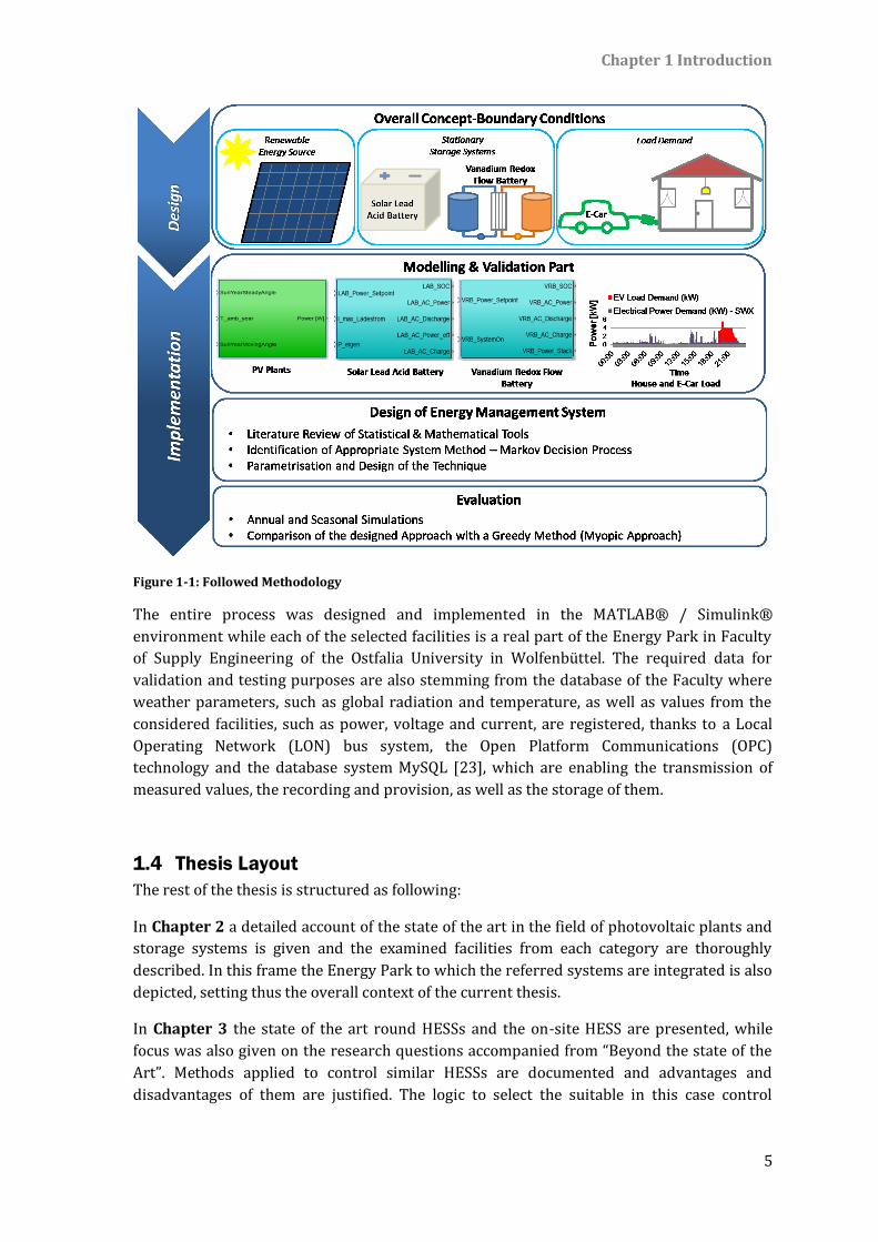
Chapter 1 Introduction
5
Figure 1-1: Followed Methodology
The entire process was designed and implemented in the MATLAB® / Simulink®
environment while each of the selected facilities is a real part of the Energy Park in Faculty
of Supply Engineering of the Ostfalia University in Wolfenbüttel. The required data for
validation and testing purposes are also stemming from the database of the Faculty where
weather parameters, such as global radiation and temperature, as well as values from the
considered facilities, such as power, voltage and current, are registered, thanks to a Local
Operating Network (LON) bus system, the Open Platform Communications (OPC)
technology and the database system MySQL [23], which are enabling the transmission of
measured values, the recording and provision, as well as the storage of them.
1.4 Thesis Layout
The rest of the thesis is structured as following:
In Chapter 2 a detailed account of the state of the art in the field of photovoltaic plants and
storage systems is given and the examined facilities from each category are thoroughly
described. In this frame the Energy Park to which the referred systems are integrated is also
depicted, setting thus the overall context of the current thesis.
In Chapter 3 the state of the art round HESSs and the on-site HESS are presented, while
focus was also given on the research questions accompanied from “Beyond the state of the
Art”. Methods applied to control similar HESSs are documented and advantages and
disadvantages of them are justified. The logic to select the suitable in this case control

Chapter 1 Introduction
6
management method is then explained while limitations of scope and challenges during the
design phase were addressed.
Chapter 4 includes the modelling part for each facility, namely the PV installation, the two
selected storage systems, the domestic loads as well as the load demand of an E-Car. In
particular, in MATLAB® / Simulink® environment all of the considered components of the
examined HESS are designed and respectively parametrized so as to depict the real facilities.
The validation was also included in the design phase by using data which are registered in
the database of the Energy Park.
Consequently the methodology chosen to control the two storage systems is explained in
detail and the applied technique is fully described in Chapter 5. The problematic which
arose during the design phase relating to the efficiency grade of the storage systems is
referred and the decided approach is justified. In addition the greedy method which will be
used as benchmark to evaluate the extracted results is also analysed and the differences
with the designed control technique are documented.
In Chapter 6 the annual and seasonal simulation results are included while the evaluation is
performed by comparing the outputs with the ones extracted for an analogous naive
approach. Comparison is not only made between the selected evaluation criteria which are
considered the metric for assessing the optimal method but also with graphical
representation of the systems which operate with a stand-alone battery and hybrid ones
and it is justified why the developed Markov method outperforms the others.
Finally in Chapter 7 the examined concept and the contribution of the thesis are
summarized while suggestions for future work are mentioned.
Chapter 2 System Fundamentals & Experimental Setting
7
2 System Fundamentals & Experimental Setting In the previous chapter an introduction to the thematic of the current thesis was presented
through setting the boundary conditions and concretizing the topic. The motivation for
handling such a domain and the specific objectives which are related to it are described
while emphasis is also given on the followed methodology, which is explained. This Section
is primarily devoted to describe the facilities which exist in the Energy Park of the Ostfalia
University and are to be integrated in the designed HES. Beside that the state of the art
around photovoltaics, storage technologies and load profiles applied, which are considered
the fundamental components of this study is to be outlined.
2.1 Energy Park of the Ostfalia University
In order to create a research test bed of a hybrid energy system on which various
measurements and different topologies can be examined so as to emulate a semi-
autonomous residence, a modular energy park was designed and gradually developed at the
premises of the Faculty of Supply Engineering at the Ostfalia University. It is composed of
RESs, storage systems and loads that can imitate the power consumption and cover the
electrical demand of a residence. The individual components are depicted in Figure 2-1,
while the interconnection among the different systems is also represented with lines
between them. It is to be noted that the selected units are appropriate for residential
purposes and the applied topology is three-phase AC. Although the examined synthesis is
used for experimental purposes, all constituent parts are commercially available.
Chapter 2 System Fundamentals & Experimental Setting
8
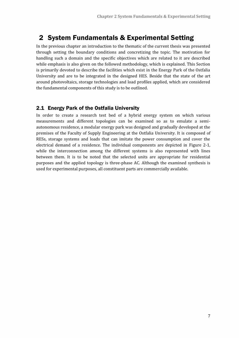
Figure 2-1: Graphical Representation of the Energy Park [18]
In particular, the available on-site devices are two PV plants of 5.1 kWp and 1.02 kWp peak
power, a wind turbine of 4 kW, a combined heat and power system (CHP) of 6 kWel and 16
kWther, a fuel cell of 1.2 kW, an electrolyser (6 kW) with a hydrogen store unit, a vanadium
redox flow battery (VRB) of 5 kW, a solar lead acid battery system (LAB) of 6 kW, a charging
station for E-Vehicles and programmable loads that can be respectively controlled to imitate
house load profiles. However, from the installed facilities not all have been integrated to the
examined study case. The photovoltaic plants, the vanadium redox flow battery, the solar
lead acid battery and the E-Vehicle are those which were adapted in the examined concept
in the framework of this thesis, with upper target to investigate under which circumstances
it is optimal to operate two storage systems for covering local demands of a residence with
an E-Vehicle, by exploiting maximally the locally produced renewable energy. It is to be
noted that since the installed facilities are connected in such a way that may operate as part
of the described system, as well as elements of a configuration with partial exploitation of
the available facilities or as stand-alone systems, no disorders or malfunctions have arisen.
The described interconnected system is supported also from a LON (Local Operating
Network) based data acquisition with a sampling rate of 1 sec and a weather station is also
integrated so as to extract weather data, useful for validation and testing purposes.
Chapter 2 System Fundamentals & Experimental Setting
9
2.2 Solar Photovoltaic Systems
PV Trend
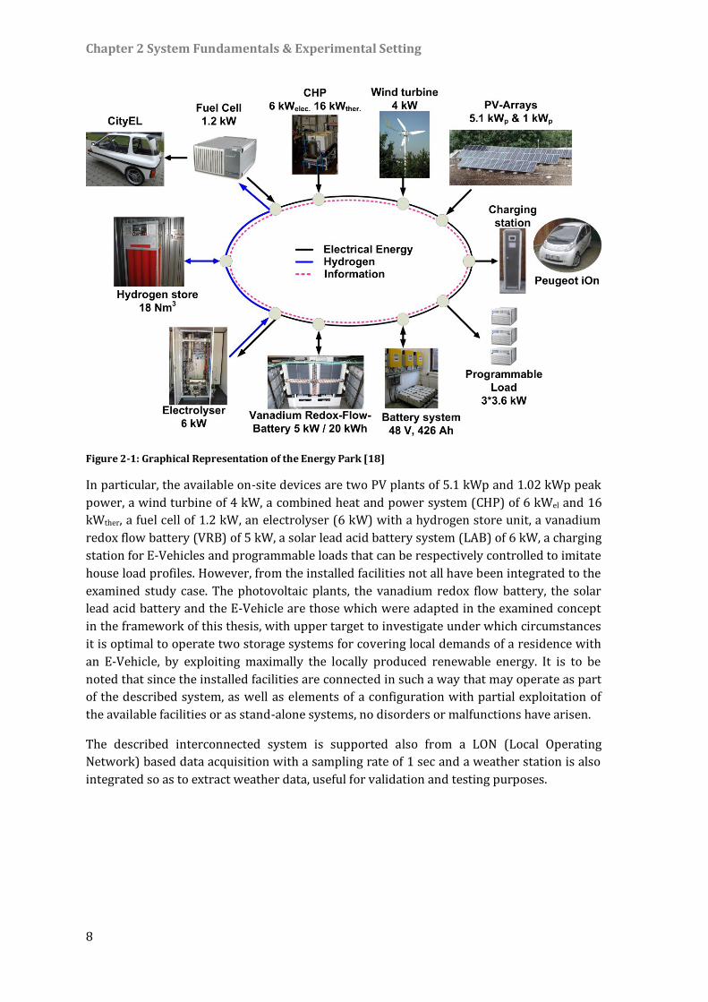
As mentioned in previous Section, PV power generation is a widespread tactic nowadays. In
Germany over 1.5 million of solar photovoltaic systems have already been installed which
are equivalent to 39.8 GWp installed power and 38.7 TWh electricity production. In the
South and West the majority of the systems are rooftop plants while in the East and North
large photovoltaic parks have been built [24]. In Figure 2-2 the PV evolution of the installed
facilities among the last fifteen years in Germany is depicted.
Figure 2-2: PV Data in Germany during the last 15 years [25]
It is obvious that the widespread installation of PV systems took place after the 1st
Renewable Energy Sources Act (Erneuerbare-Energien-Gesetz) came into force in 2000. The
introduced favorable feed-in-tariffs contributed to the exponential interest of the public and
soon the installation of a PV system on the house rooftop turned out to be a profitable
investment.
In the next sections the state of the art around the PV technology and the integrated to the
examined HESS PV facility are explained in detail.
2.2.1 State of the Art of Photovoltaic
Solar energy is indefinite, renewable and sustainable, as well as one of the most abundant
sources that can be used to produce heat or electricity. Photovoltaic systems can transform
via solar panels solar energy into electricity by exploiting the photoelectric effect. According
to this phenomenon, electrons are dislodged from a pn junction when light under specific
circumstances hits the material. This movement of electrons is actually the physical
representation of electricity.
The main components of the photovoltaic systems are the panels, which are connected in
series to achieve the anticipated output voltage, or in parallel to reach the required current
level. Panels are formed from one or more modules, and are preassembled, while modules
0
5
10
15
20
25
30
35
40
0
5
10
15
20
25
30
35
40
1990
1991
1992
1993
1994
1995
1996
1997
1998
1999
2000
2001
2002
2003
2004
2005
2006
2007
2008
2009
2010
2011
2012
2013
2014
2015
Gro
ss E
lect
rici
ty P
rod
uct
ion
in T
Wh
Inst
alle
d P
ow
er
in G
W
Year
Installed PV Power in Germany Annual Gross Electricity Production
Chapter 2 System Fundamentals & Experimental Setting
10
consist of the PV cells, which are the semiconductor units that convert the incident
irradiance into electricity. Since the produced current is direct, an inverter is in most cases
required to convert it in alternating current.
Different types of PV cells have reached commercial maturity to form the PV modules and
panels consequently. These are described by the following clusters:
Monocrystalline PV Cells: They are considered the most effective technology of all but
also the most expensive, since cells must be sliced into wafers resulting to a high waste
of material, if it is considered that during the process almost 50% of it is turned into
dust [26]. Typically over 16% of the solar irradiance is converted into electricity [27].
Polycrystalline PV Cells: These cells consist of multiple layers of crystal which are grown
between the material. The deficit of such a technique is though that the area between
the formed layers creates resistance thus its performance deteriorates (almost 15%
efficiency) [27].
Thin Film PV Cells: The thin film PV cells are made by depositing silicon on a thin surface
which can be glass, or other material so as to form the solar module. They are
characterized by a lower efficiency (6%-11%) [27], though their production is simpler
and cheaper [28].
Organic PV Cells: They take advantage of organic electronics to produce electricity from
the photovoltaic effect and their low cost manufacturing increases their potential
application in the future. However the low efficiency (~10%) and the duration still
inhibit a broader employment [29].
Hybrid PV Cells: This type of solar cells combines organic and inorganic components. In
particular, the parts that absorb light are made from polymers while the surface which
receives the excited electrons is made from inorganic materials. It is a promising
technique that has already high efficiency grades achieved at experimental stage
(~40%) [29].
For household installations, since the space capacity is usually limited it is thoughtful to
install panels with a higher efficiency grade so as to achieve a higher gain and consequently
lower installation costs. On the other hand, when solar parks are planned on land areas the
efficiency grade is not that important.
The rooftop installations use building mounted solar arrays. The tilt angle of the panels is
calculated based on the specific constructional characteristics as well as on the site of the
building. When referring to ground-mounted systems, different installation structures can
be applied, in order to increase the incident angle of the sun on the panels:
Fixed arrays: With a fixed angle towards the south and a tilt angle usually smaller than
the latitude of the installation area, so as to achieve the maximum annual power yield,
this type of structure is widespread due to its low installation costs and simplicity in
manufacturing. The tilt angle can also be monthly manually adjusted, benefiting from
seasonal changes.
Single axis trackers: This cluster of floating mount foundation includes the trackers with
one degree of freedom, which is represented from one axis that can rotate. They favor
the tracking of sun’s movement during the day but they are unable to modify their angle
Chapter 2 System Fundamentals & Experimental Setting
11
adjusting to seasonal changes. Their performance can be increased up to 30% over the
static panels [30, 31].
Dual axis trackers: Target of those systems is to follow sun’s orbit during the day and
yearly. With the primary and secondary axis they can angle themselves so as to have
always the optimum orientation. Their added complexity in manufacturing is however
not always worthwhile, since it is proved that only an added performance of 6% from
the single axis trackers are noted [30, 31].
The best technique to be applied depends on various factors such as the installation site, the
size of the planned solar park, the weather conditions of the area etc.. A higher investment
cost for installing dual axis trackers may ultimately not yield the expected profit in the
annual energy collection. So a systematic analysis is required and several aspects are to be
taken into account before concluding to a specific mounting system.
Finally, another categorization of photovoltaic systems is between grid-connected or stand-
alone systems which operate in island mode. Grid-connected systems are connected to the
public power grid while those in island operation are feeding the produced energy only to
on-site loads or to installed storage systems.
The characteristic I-V curve of the PV cells is an additional significant attribute of the
respective facility. Given a steady solar irradiance and a steady temperature there is always
a point on the curve which yields the highest output power. This point is called Maximum
Power Point (MPP) and target is to operate always the system at this power point. This is
succeeded via varying the resistance in the PV circuit which consequently influences the
voltage and current level.
2.2.2 Description of the on-site Phovoltaic (PV) installation
The PV installation which is considered as the RES for the hybrid system is compiled from
two smaller PV plants of 5.1kW and 1.02kW (Figure 2-3). These plants exist both in the
facilities of the Laboratory for Electrical Engineering and Renewable Energy Systems and
have been installed at the roof top of the Faculty of Supply Engineering at the Ostfalia
University of Applied Sciences in Wolfenbüttel.
Figure 2-3: The installed PV Power plants of (a) 5.1kWp Plant with 30 modules; (b) 1.02kWp Plant with 12 modules
The 1st Plant with installed power of 5.1 kW is consisting of two strings of 30 modules each.
Each string consists also of two times of 15 modules in series and then in parallel connected.
The module is composed of 36 monocrystalline cells from the BP company and each cell has
Chapter 2 System Fundamentals & Experimental Setting
12
a maximum power (𝑃𝑚𝑎𝑥) of 85 W. In Table 2-1 manufacturer’s specifications of the
installed PV modules are given. The solar panels are south oriented with a fixed angle to the
ground of 30o and the plant is connected to the grid via 2 string inverters Sunny Boy 2000
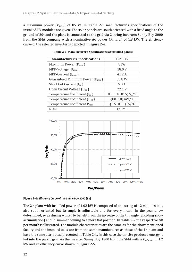
from the SMA company with a nominative AC power (𝑃𝐴𝐶𝑛𝑜𝑚) of 1.8 kW. The efficiency
curve of the selected inverter is depicted in Figure 2-4.
Table 2-1: Manufacturer’s Specifications of installed panels
Manufacturer’s Specifications BP 585
Maximum Power (Pmax ) 85W
MPP-Votlage (Umpp ) 18.0 V
MPP-Current (lmpp ) 4.72 A
Guaranteed Minimum Power (Pmin ) 80.8 W
Short Cut Current (Isc ) 5.0 A
Open Circuit Voltage (Uoc ) 22.1 V
Temperature Coefficient (lsc ) (0.065±0.015) %/°C
Temperature Coefficient (Uoc ) -(80±10) mV/°C
Temperature Coefficient Pmax -(0.5±0.05) %/°C
NOCT 47±2°C
Figure 2-4: Efficiency Curve of the Sunny Boy 2000 [32]
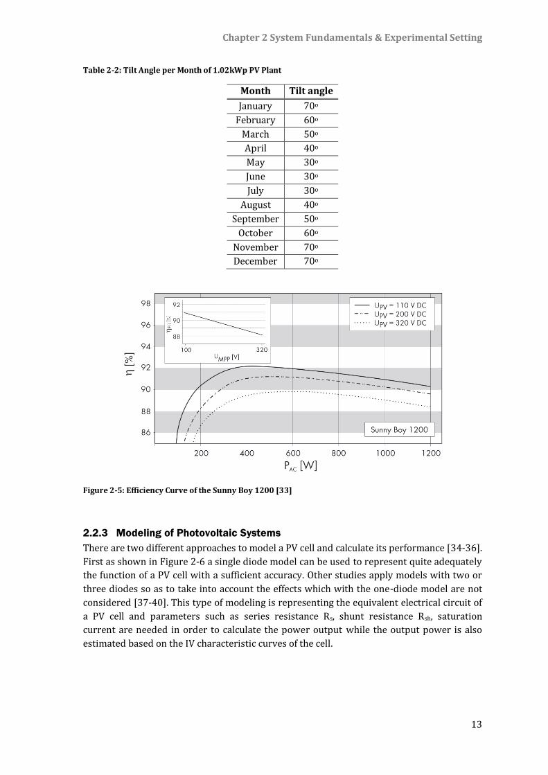
The 2nd plant with installed power of 1.02 kW is composed of one string of 12 modules, it is
also south oriented but its angle is adjustable and for every month in the year anew
determined, so as during winter to benefit from the increase of the tilt angle (avoiding snow
accumulation) and in summer coming to a more flat position. In Table 2-2 the respective tilt
per month is illustrated. The module characteristics are the same as for the abovementioned
facility and the installed cells are from the same manufacturer as these of the 1st plant and
have the same attributes, presented in Table 2-1. In this case the on-site produced energy is
fed into the public grid via the Inverter Sunny Boy 1200 from the SMA with a 𝑃𝐴𝐶𝑛𝑜𝑚 of 1.2
kW and an efficiency curve shown in Figure 2-5.
Chapter 2 System Fundamentals & Experimental Setting
13
Table 2-2: Tilt Angle per Month of 1.02kWp PV Plant
Month Tilt angle
January 70o
February 60o
March 50o
April 40o
May 30o
June 30o
July 30o
August 40o
September 50o
October 60o
November 70o
December 70o
Figure 2-5: Efficiency Curve of the Sunny Boy 1200 [33]
2.2.3 Modeling of Photovoltaic Systems
There are two different approaches to model a PV cell and calculate its performance [34-36].
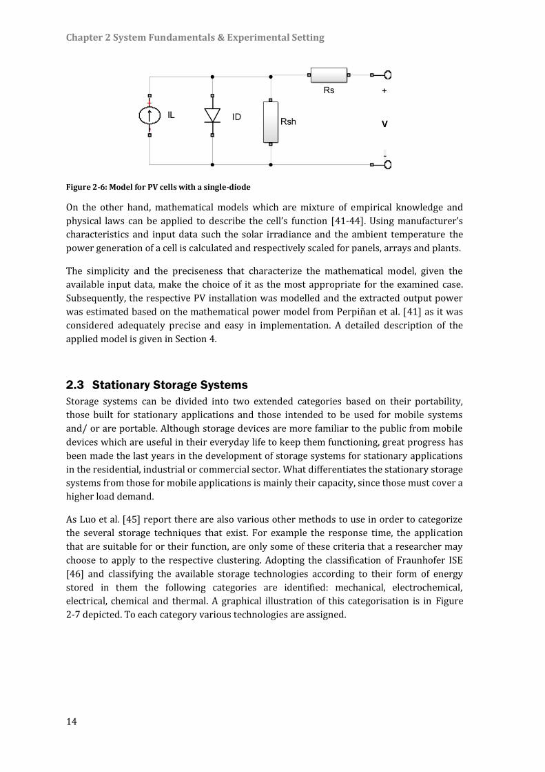
First as shown in Figure 2-6 a single diode model can be used to represent quite adequately
the function of a PV cell with a sufficient accuracy. Other studies apply models with two or
three diodes so as to take into account the effects which with the one-diode model are not
considered [37-40]. This type of modeling is representing the equivalent electrical circuit of
a PV cell and parameters such as series resistance Rs, shunt resistance Rsh, saturation
current are needed in order to calculate the power output while the output power is also
estimated based on the IV characteristic curves of the cell.
Chapter 2 System Fundamentals & Experimental Setting
14
Figure 2-6: Model for PV cells with a single-diode
On the other hand, mathematical models which are mixture of empirical knowledge and
physical laws can be applied to describe the cell’s function [41-44]. Using manufacturer’s
characteristics and input data such the solar irradiance and the ambient temperature the
power generation of a cell is calculated and respectively scaled for panels, arrays and plants.
The simplicity and the preciseness that characterize the mathematical model, given the
available input data, make the choice of it as the most appropriate for the examined case.
Subsequently, the respective PV installation was modelled and the extracted output power
was estimated based on the mathematical power model from Perpiñan et al. [41] as it was
considered adequately precise and easy in implementation. A detailed description of the
applied model is given in Section 4.
2.3 Stationary Storage Systems
Storage systems can be divided into two extended categories based on their portability,
those built for stationary applications and those intended to be used for mobile systems
and/ or are portable. Although storage devices are more familiar to the public from mobile
devices which are useful in their everyday life to keep them functioning, great progress has
been made the last years in the development of storage systems for stationary applications
in the residential, industrial or commercial sector. What differentiates the stationary storage
systems from those for mobile applications is mainly their capacity, since those must cover a
higher load demand.
As Luo et al. [45] report there are also various other methods to use in order to categorize
the several storage techniques that exist. For example the response time, the application
that are suitable for or their function, are only some of these criteria that a researcher may
choose to apply to the respective clustering. Adopting the classification of Fraunhofer ISE
[46] and classifying the available storage technologies according to their form of energy
stored in them the following categories are identified: mechanical, electrochemical,
electrical, chemical and thermal. A graphical illustration of this categorisation is in Figure
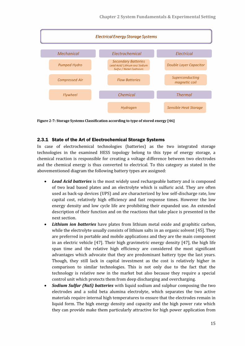
2-7 depicted. To each category various technologies are assigned.
Chapter 2 System Fundamentals & Experimental Setting
15
Figure 2-7: Storage Systems Classification according to type of stored energy [46]
2.3.1 State of the Art of Electrochemical Storage Systems
In case of electrochemical technologies (batteries) as the two integrated storage
technologies in the examined HESS topology belong to this type of energy storage, a
chemical reaction is responsible for creating a voltage difference between two electrodes
and the chemical energy is thus converted to electrical. To this category as stated in the
abovementioned diagram the following battery types are assigned:
Lead Acid batteries is the most widely used rechargeable battery and is composed
of two lead based plates and an electrolyte which is sulfuric acid. They are often
used as back-up devices (UPS) and are characterized by low self-discharge rate, low
capital cost, relatively high efficiency and fast response times. However the low
energy density and low cycle life are prohibiting their expanded use. An extended
description of their function and on the reactions that take place is presented in the
next section.
Lithium ion batteries have plates from lithium metal oxide and graphitic carbon,
while the electrolyte usually consists of lithium salts in an organic solvent [45]. They
are preferred in portable and mobile applications and they are the main component
in an electric vehicle [47]. Their high gravimetric energy density [47], the high life
span time and the relative high efficiency are considered the most significant
advantages which advocate that they are predominant battery type the last years.
Though, they still lack in capital investment as the cost is relatively higher in
comparison to similar technologies. This is not only due to the fact that the
technology is relative new in the market but also because they require a special
control unit which protects them from deep discharging and overcharging.
Sodium Sulfur (NaS) batteries with liquid sodium and sulphur composing the two
electrodes and a solid beta alumina electrolyte, which separates the two active
materials require internal high temperatures to ensure that the electrodes remain in
liquid form. The high energy density and capacity and the high power rate which
they can provide make them particularly attractive for high power application from
Chapter 2 System Fundamentals & Experimental Setting
16
utilities or large consumers [47]. One special characteristic of this type of storage
system is that the utilized materials are fully recyclable, setting their disposal as
environmental friendly. The high operational and capital cost as well as the need for
a heat source which is needed for operating the system are on the other hand
included in the drawbacks of such systems.
Nickel Cadmium (NiCd) batteries are considered a mature technology and have
been commercially available already from the beginning of the last century.
Electrodes’ materials are nickel hydroxide and metallic cadmium while the
electrolyte is an aqueous solution [45]. Their capability to operate efficiently under
low temperatures makes them competitive in the storage market and their low
maintenance cost is contributing to their employment in storage applications.
However, the high toxicity of the used materials as well as the memory effect which
characterizes the battery are the most important disadvantages of those systems.
Although flow batteries are characterized by similar chemical reactions as in the
conventional battery systems, the storing technique of the electrolyte is the attribute that
differentiates them [48]. The electrolyte is stored in external tanks and through pipes is
driven to the cell stack and circulated where the voltage difference is created. Their main
asset is that the power and capacity are independently scalable, thus providing a flexible
dimensioning of the facility according to the needs of the respective customer. On the
contrary they have a high constructional complexity and the capital cost to obtain them
remains relatively high. Different configurations of flow batteries are reported with main
difference in the species in the anolyte and catholyte. Main types are the vanadium redox
flow (which have the same species but different oxidation states) and the hybrid ones [49].
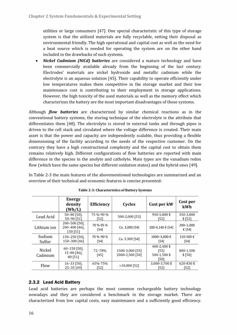
In Table 2-3 the main features of the abovementioned technologies are summarized and an
overview of their technical and economic features is concise presented:
Table 2-3: Characteristics of Battery Systems
Energy density (Wh/L)
Efficiency Cycles Cost per kW Cost per
kWh
Lead Acid 50–80 [50], 50–90 [51]
75 %-90 % [52]
500-2,000 [53] 950-5,800 $
[52] 350-3,800
$ [52]
Lithium ion 200–500 [50], 200–400 [46],
150 [51]
70 %-95 % [54]
Ca. 3,000 [54] 200-4,140 € [54] 200–1,000
€ [54]
Sodium Sulfur
150–250 [50], 150–300 [46]
70 %–90 % [54]
Ca. 3,300 [54] 1000–3,000 €
[54] 210-500 €
[54]
Nickel Cadmium
60–150 [50], 15–80 [46],
80 [51]
72–78% [45]
1500-3,000 [55] 2000-2,500 [50]
400-2,400 $ [55]
500-1,500 $ [50]
800-1,500 $ [50]
Flow 16–33 [50], 25–35 [49]
65%-75% [52]
>10,000 [52] 3,000-3,700 $
[52] 620-830 $
[52]
2.3.2 Lead Acid Battery
Lead acid batteries are perhaps the most common rechargeable battery technology
nowadays and they are considered a benchmark in the storage market. There are
characterized from low capital costs, easy maintenance and a sufficiently good efficiency.
Chapter 2 System Fundamentals & Experimental Setting
17
However their short life cycle due to accumulative deposition of lead sulphate on the
electrodes and their limited energy density has forced the market in research and
development of other storage technologies which could replace it [56]. Nevertheless, it
remains dominant in the storage market although various other types have been
commercial and technological mature.
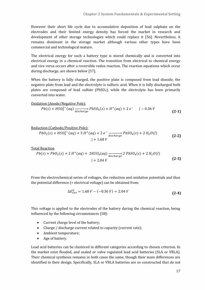
The electrical energy for such a battery type is stored chemically and is converted into
electrical energy in a chemical reaction. The transition from electrical to chemical energy
and vice versa occurs after a reversible redox reaction. The reaction equations which occur
during discharge, are shown below [57].
When the battery is fully charged, the positive plate is composed from lead dioxide, the
negative plate from lead and the electrolyte is sulfuric acid. When it is fully discharged both
plates are composed of lead sulfate (PbSO4), while the electrolyte has been primarily
converted into water.
Oxidation (Anode/Negative Pole):
𝑃𝑏(𝑠) + 𝐻𝑆𝑂42−(𝑎𝑞)
𝑑𝑖𝑠𝑐ℎ𝑎𝑟𝑔𝑒→ 𝑃𝑏𝑆𝑂4(𝑠) + 𝐻
+(𝑎𝑞) + 2 𝑒− | − 0.36 𝑉 (2-1)
Reduction (Cathode/Positive Pole):
𝑃𝑏𝑂2(𝑠) + 𝐻𝑆𝑂42−(𝑎𝑞) + 3 𝐻+(𝑎𝑞) + 2 𝑒−
𝑑𝑖𝑠𝑐ℎ𝑎𝑟𝑔𝑒→ 𝑃𝑏𝑆𝑂4(𝑠) + 2 𝐻2𝑂(𝑙)
| + 1.68 𝑉 (2-2)
Total Reaction
𝑃𝑏(𝑠) + 𝑃𝑏𝑂2(𝑠) + 2 𝐻+(𝑎𝑞) + 2𝐻𝑆𝑂4(𝑎𝑞)
𝑑𝑖𝑠𝑐ℎ𝑎𝑟𝑔𝑒→ 2 𝑃𝑏𝑆𝑂4(𝑠) + 2 𝐻2𝑂(𝑙)
| + 2.04 𝑉 (2-3)
From the electrochemical series of voltages, the reduction and oxidation potentials and thus
the potential difference (= electrical voltage) can be obtained from:
Δ𝐸𝐺𝑒𝑠0 = 1.68 𝑉 − (−0.36 𝑉) = 2.04 𝑉 (2-4)
This voltage is applied to the electrodes of the battery during the chemical reaction, being
influenced by the following circumstances [58]:
Current charge level of the battery;
Charge / discharge current related to capacity (current rate);
Ambient temperature;
Age of battery.
Lead acid batteries can be clustered in different categories according to chosen criterion. In
the market exist flooded, and sealed or valve regulated lead acid batteries (SLA or VRLA).
Their chemical synthesis remains in both cases the same, though their main differences are
identified in their design. Specifically, SLA or VRLA batteries are so constructed that do not
Chapter 2 System Fundamentals & Experimental Setting
18
need topping up of electrolyte, they do not require regular ventilation of produced hydrogen
and they are in total low-maintenance systems, in contrast to flooded batteries which need
all the above mentioned services to operate optimally [59-60].
Moreover SLA or VRLA batteries are classified in wet, gel and absorbed glass mat (AGM)
type. Wet type batteries are normally characterized from low cycle life but also low price.
AGM and gel type differ from each other in the storage composition of the electrolyte.
Usually AGM are less durable in deep discharge and have a shorter cycle life than gel type
[60].
One last categorization is between deep cycle and shallow cycle lead acid batteries. As their
name indicates the first may be deeply discharged without damaging the battery, though
being able to provide lower rate but for longer time period. The second type is preferred in
automotive field for starting engines and ignition purposes producing higher currents in
shorter time.
2.3.2.1 Description of the on-site Lead Acid Battery
The battery system to be integrated in the HESS belongs to the renewable energy park of the
Ostfalia University of Applied Sciences in Wolfenbüttel. Theoretically, it could serve as an
electrical buffer storage system, which will shave load peaks and store excess energy. In
practice, however, it is used only for experimental purposes and is charged from renewable
energy generators (photovoltaic systems, wind turbine, combined heat and power plant)
and from public grid [58].
This solar lead acid gel battery is composed of blocks from HOPPECKE, with a deeper
discharging capability and technological maturity to charge with low current levels. The
electrolyte between the plates is in gel form avoiding the gassing effect and leading to lower
maintenance costs.
The system consists of 16 interconnected 6V lead-gel battery blocks with a single capacity of
229 Ah at a 10-hour discharge rate (C10). In this case, always eight batteries are connected in
series (two rows) so that the total battery voltage is UN = 8 x 6 V = 48 V. The charge rate C
(in Ah) is increased by the parallel circuit so that the two rows lead to a total nominal
capacity of CN = 2 x 229 Ah = 458 Ah. With the nominal voltage of Unom = 48 V, the storable
energy of the battery system is:
𝐸𝑒𝑙 = 458𝐴ℎ × 48𝑉 = 21.98 𝑘𝑊ℎ (2-5)
Since the energy park is constructed on a three-phase AC topology, the battery system is
connected to the energy park via three bidirectional inverters SUNNY BACKUP 5000 with an
Automatic Switchbox from SMA (Figure 2-8), so that the current is inverted in direct form
when battery is being charged and back into three-phase alternating current which can be
fed to cover the load demand when it is being discharged [58].
The charging process of the battery is controlled from the inverters starting with a constant
current charge (Constant Current Mode) and going into a constant voltage charge (Constant
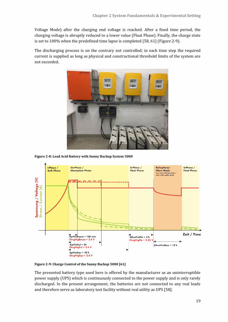
Chapter 2 System Fundamentals & Experimental Setting
19
Voltage Mode) after the charging end voltage is reached. After a fixed time period, the
charging voltage is abruptly reduced to a lower value (Float Phase). Finally, the charge state
is set to 100% when the predefined time lapse is completed [58, 61] (Figure 2-9).
The discharging process is on the contrary not controlled; in each time step the required
current is supplied as long as physical and constructional threshold limits of the system are
not exceeded.
Figure 2-8: Lead Acid Battery with Sunny Backup System 5000
Figure 2-9: Charge Control of the Sunny Backup 5000 [61]
The presented battery type used here is offered by the manufacturer as an uninterruptible
power supply (UPS) which is continuously connected to the power supply and is only rarely
discharged. In the present arrangement, the batteries are not connected to any real loads
and therefore serve as laboratory test facility without real utility as UPS [58].
Chapter 2 System Fundamentals & Experimental Setting
20
2.3.2.2 Modeling of Lead Acid Battery System
Battery models fall into different categories which include mathematical, electrochemical,
thermal and electrical models [62]. So as to describe the different processes inside a battery
various models have been developed which can be represented with equivalent circuit
diagrams. This type of models use simple components such as resistors, capacitances and
voltage sources so as to build the respective electrical behavior that matches the respective
battery. The more components (RC elements) the circuit diagram includes the more precise
it is; though it lacks in computational speed, and vice versa [58]. When adding further
parallel-connected components self-discharge effects or other capacitances are taken into
account. In general, it is important to consider how important a high accuracy is, since each
additional calculation requires further computation time [58]. In Figure 2-10 a generalized
equivalent circuit diagram with 𝑛 different RC parallel elements is depicted:
Voc
Ro
Rp1 Rpn
Cp1 Cpn
+
-
Figure 2-10: Equivalent Circuit Model for Battery
In the literature three of the most commonly applied battery models are the Resistive
Thevenin model, the Thevenin and the Linear Model [63-64] and belong to the equivalent
circuit-based models (Figure 2-11). The resistive Thevenin model [65-66] consists of an
ideal voltage source and an internal resistance. The Thevenin model [67] has additionally an
RC element, so as to take into account the delay effect caused by the capacitance of the
parallel plates. Finally the Linear Model [68] has an additional parallel connected resistor
which considers the self-discharge of the battery.
It is important in the frame of this thesis to develop/ integrate models that simulate the
performance of the existing facilities as best as possible, without neglecting the
generalization factor that has to be maintained. Trying to strike a balance between accuracy
and computational speed, it was thus decided to apply the Linear model to simulate the
performance of the existing lead acid battery, since it is considered the most complete (the
self-discharge factor is taken into account) without demanding extremely high measuring
effort to parametrize it. Its equivalent circuit model was interpreted into a mathematical
model and the respective parameters were defined after a series of experiments. However,
it is to be noted that although in the abovementioned models the resistances are assumed to
be constant, in the designed model the battery conditions were affecting their value. In
addition due to the fact that different phenomena take place during the charge and
discharge process the equivalent circuit model was designed, so as to choose in each case
the respective resistance. Finally temperature effects are not considered as the battery is
kept in a room and great variations are not noticed. For this reason a non-linear model was
excluded from this review.
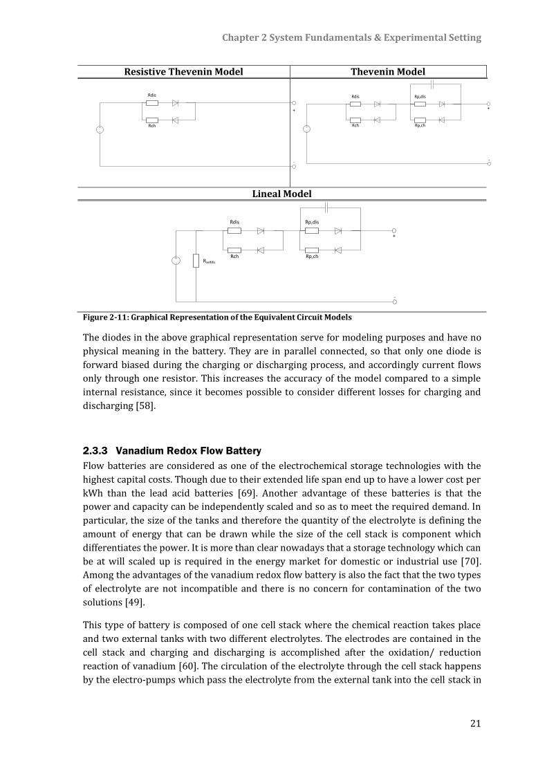
Chapter 2 System Fundamentals & Experimental Setting
21
Resistive Thevenin Model Thevenin Model
Rdis
+
-
Rch
Rdis
+
-
Rch
Rp,dis
Rp,ch
Lineal Model
Rdis
+
-
Rch
Rp,dis
Rp,chRselfdis
Figure 2-11: Graphical Representation of the Equivalent Circuit Models
The diodes in the above graphical representation serve for modeling purposes and have no
physical meaning in the battery. They are in parallel connected, so that only one diode is
forward biased during the charging or discharging process, and accordingly current flows
only through one resistor. This increases the accuracy of the model compared to a simple
internal resistance, since it becomes possible to consider different losses for charging and
discharging [58].
2.3.3 Vanadium Redox Flow Battery
Flow batteries are considered as one of the electrochemical storage technologies with the
highest capital costs. Though due to their extended life span end up to have a lower cost per
kWh than the lead acid batteries [69]. Another advantage of these batteries is that the
power and capacity can be independently scaled and so as to meet the required demand. In
particular, the size of the tanks and therefore the quantity of the electrolyte is defining the
amount of energy that can be drawn while the size of the cell stack is component which
differentiates the power. It is more than clear nowadays that a storage technology which can
be at will scaled up is required in the energy market for domestic or industrial use [70].
Among the advantages of the vanadium redox flow battery is also the fact that the two types
of electrolyte are not incompatible and there is no concern for contamination of the two
solutions [49].
This type of battery is composed of one cell stack where the chemical reaction takes place
and two external tanks with two different electrolytes. The electrodes are contained in the
cell stack and charging and discharging is accomplished after the oxidation/ reduction
reaction of vanadium [60]. The circulation of the electrolyte through the cell stack happens
by the electro-pumps which pass the electrolyte from the external tank into the cell stack in
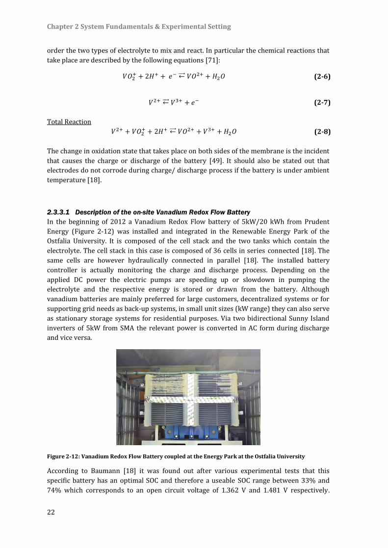
Chapter 2 System Fundamentals & Experimental Setting
22
order the two types of electrolyte to mix and react. In particular the chemical reactions that
take place are described by the following equations [71]:
𝑉𝑂2+ + 2𝐻+ + 𝑒− ←⃗⃗⃗ 𝑉𝑂2+ + 𝐻2𝑂 (2-6)
𝑉2+ ←⃗⃗⃗ 𝑉3+ + 𝑒− (2-7)
Total Reaction
𝑉2+ + 𝑉𝑂2+ + 2𝐻+ ←⃗⃗⃗ 𝑉𝑂2+ + 𝑉3+ +𝐻2𝑂 (2-8)
The change in oxidation state that takes place on both sides of the membrane is the incident
that causes the charge or discharge of the battery [49]. It should also be stated out that
electrodes do not corrode during charge/ discharge process if the battery is under ambient
temperature [18].
2.3.3.1 Description of the on-site Vanadium Redox Flow Battery
In the beginning of 2012 a Vanadium Redox Flow battery of 5kW/20 kWh from Prudent
Energy (Figure 2-12) was installed and integrated in the Renewable Energy Park of the
Ostfalia University. It is composed of the cell stack and the two tanks which contain the
electrolyte. The cell stack in this case is composed of 36 cells in series connected [18]. The
same cells are however hydraulically connected in parallel [18]. The installed battery
controller is actually monitoring the charge and discharge process. Depending on the
applied DC power the electric pumps are speeding up or slowdown in pumping the
electrolyte and the respective energy is stored or drawn from the battery. Although
vanadium batteries are mainly preferred for large customers, decentralized systems or for
supporting grid needs as back-up systems, in small unit sizes (kW range) they can also serve
as stationary storage systems for residential purposes. Via two bidirectional Sunny Island
inverters of 5kW from SMA the relevant power is converted in AC form during discharge
and vice versa.
Figure 2-12: Vanadium Redox Flow Battery coupled at the Energy Park at the Ostfalia University
According to Baumann [18] it was found out after various experimental tests that this
specific battery has an optimal SOC and therefore a useable SOC range between 33% and
74% which corresponds to an open circuit voltage of 1.362 V and 1.481 V respectively.
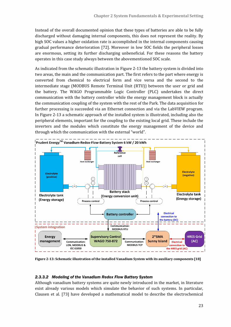
Chapter 2 System Fundamentals & Experimental Setting
23
Instead of the overall documented opinion that these types of batteries are able to be fully
discharged without damaging internal components, this does not represent the reality. By
high SOC values a higher oxidation rate is accomplished in the internal components causing
gradual performance deterioration [72]. Moreover in low SOC fields the peripheral losses
are enormous, setting its further discharging unbeneficial. For these reasons the battery
operates in this case study always between the abovementioned SOC scale.
As indicated from the schematic illustration in Figure 2-13 the battery system is divided into
two areas, the main and the communication part. The first refers to the part where energy is
converted from chemical to electrical form and vice versa and the second to the
intermediate stage (MODBUS Remote Terminal Unit (RTU)) between the user or grid and
the battery. The WAGO Programmable Logic Controller (PLC) undertakes the direct
communication with the battery controller while the energy management block is actually
the communication coupling of the system with the rest of the Park. The data acquisition for
further processing is succeeded via an Ethernet connection and via the LabVIEW program.
In Figure 2-13 a schematic approach of the installed system is illustrated, including also the
peripheral elements, important for the coupling to the existing local grid. These include the
inverters and the modules which constitute the energy management of the device and
through which the communication with the external “world”.
Figure 2-13: Schematic illustration of the installed Vanadium System with its auxiliary components [18]
2.3.3.2 Modeling of the Vanadium Redox Flow Battery System
Although vanadium battery systems are quite newly introduced in the market, in literature
exist already various models which simulate the behavior of such systems. In particular,
Clausen et al. [73] have developed a mathematical model to describe the electrochemical
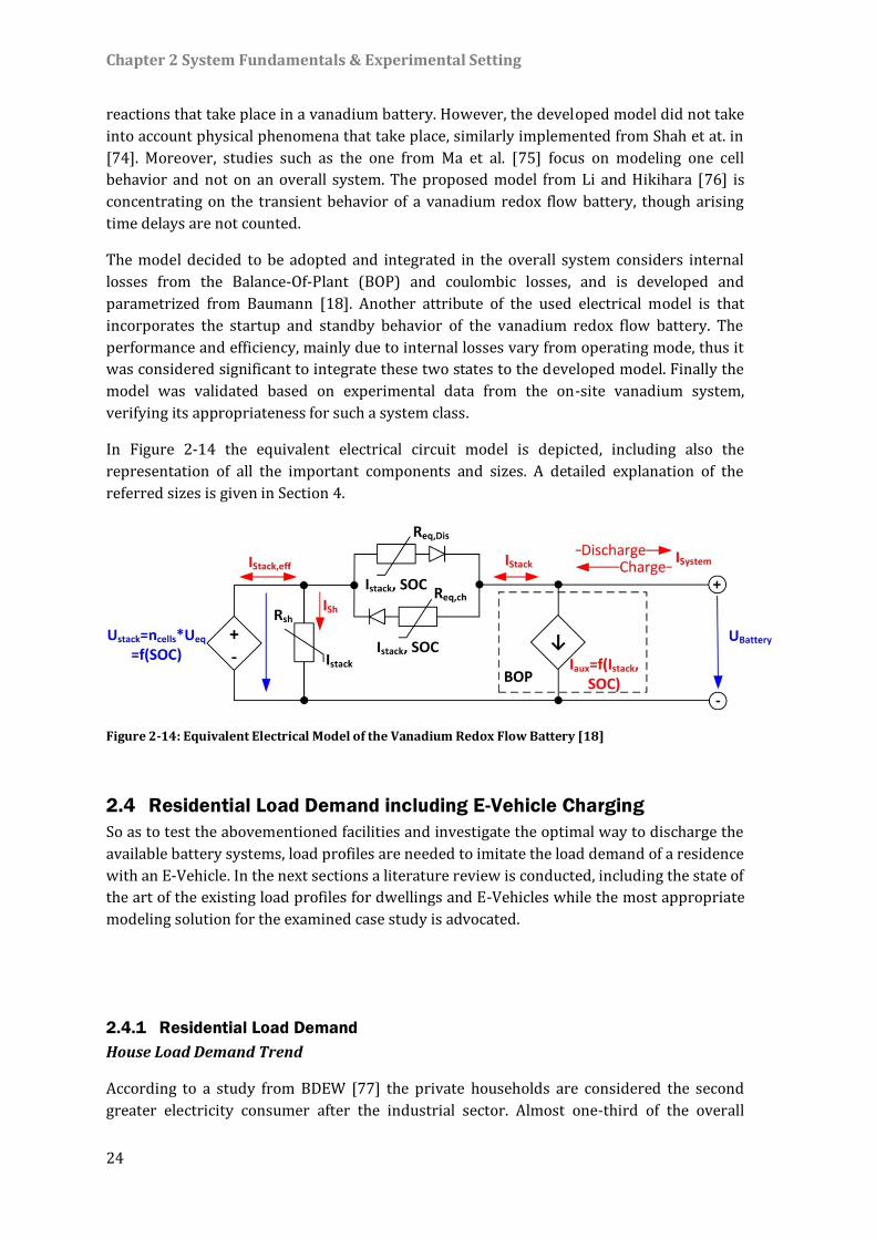
Chapter 2 System Fundamentals & Experimental Setting
24
reactions that take place in a vanadium battery. However, the developed model did not take
into account physical phenomena that take place, similarly implemented from Shah et at. in
[74]. Moreover, studies such as the one from Ma et al. [75] focus on modeling one cell
behavior and not on an overall system. The proposed model from Li and Hikihara [76] is
concentrating on the transient behavior of a vanadium redox flow battery, though arising
time delays are not counted.
The model decided to be adopted and integrated in the overall system considers internal
losses from the Balance-Of-Plant (BOP) and coulombic losses, and is developed and
parametrized from Baumann [18]. Another attribute of the used electrical model is that
incorporates the startup and standby behavior of the vanadium redox flow battery. The
performance and efficiency, mainly due to internal losses vary from operating mode, thus it
was considered significant to integrate these two states to the developed model. Finally the
model was validated based on experimental data from the on-site vanadium system,
verifying its appropriateness for such a system class.
In Figure 2-14 the equivalent electrical circuit model is depicted, including also the
representation of all the important components and sizes. A detailed explanation of the
referred sizes is given in Section 4.
Figure 2-14: Equivalent Electrical Model of the Vanadium Redox Flow Battery [18]
2.4 Residential Load Demand including E-Vehicle Charging
So as to test the abovementioned facilities and investigate the optimal way to discharge the
available battery systems, load profiles are needed to imitate the load demand of a residence
with an E-Vehicle. In the next sections a literature review is conducted, including the state of
the art of the existing load profiles for dwellings and E-Vehicles while the most appropriate
modeling solution for the examined case study is advocated.
2.4.1 Residential Load Demand
House Load Demand Trend
According to a study from BDEW [77] the private households are considered the second
greater electricity consumer after the industrial sector. Almost one-third of the overall
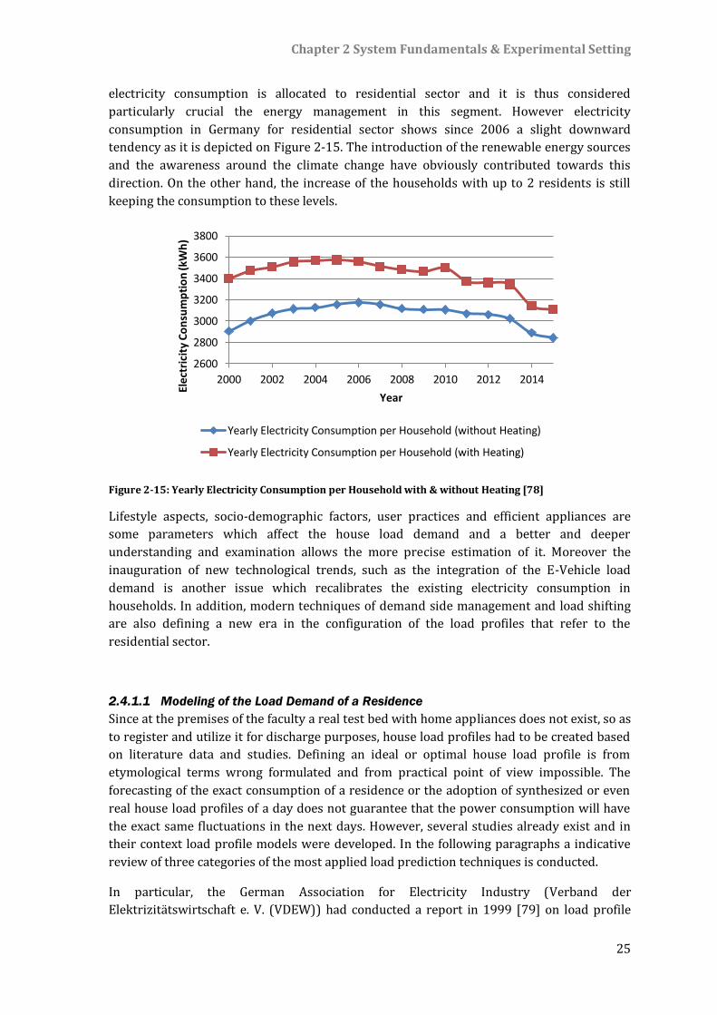
Chapter 2 System Fundamentals & Experimental Setting
25
electricity consumption is allocated to residential sector and it is thus considered
particularly crucial the energy management in this segment. However electricity
consumption in Germany for residential sector shows since 2006 a slight downward
tendency as it is depicted on Figure 2-15. The introduction of the renewable energy sources
and the awareness around the climate change have obviously contributed towards this
direction. On the other hand, the increase of the households with up to 2 residents is still
keeping the consumption to these levels.
Figure 2-15: Yearly Electricity Consumption per Household with & without Heating [78]
Lifestyle aspects, socio-demographic factors, user practices and efficient appliances are
some parameters which affect the house load demand and a better and deeper
understanding and examination allows the more precise estimation of it. Moreover the
inauguration of new technological trends, such as the integration of the E-Vehicle load
demand is another issue which recalibrates the existing electricity consumption in
households. In addition, modern techniques of demand side management and load shifting
are also defining a new era in the configuration of the load profiles that refer to the
residential sector.
2.4.1.1 Modeling of the Load Demand of a Residence
Since at the premises of the faculty a real test bed with home appliances does not exist, so as
to register and utilize it for discharge purposes, house load profiles had to be created based
on literature data and studies. Defining an ideal or optimal house load profile is from
etymological terms wrong formulated and from practical point of view impossible. The
forecasting of the exact consumption of a residence or the adoption of synthesized or even
real house load profiles of a day does not guarantee that the power consumption will have
the exact same fluctuations in the next days. However, several studies already exist and in
their context load profile models were developed. In the following paragraphs a indicative
review of three categories of the most applied load prediction techniques is conducted.
In particular, the German Association for Electricity Industry (Verband der
Elektrizitätswirtschaft e. V. (VDEW)) had conducted a report in 1999 [79] on load profile
2600
2800
3000
3200
3400
3600
3800
2000 2002 2004 2006 2008 2010 2012 2014
Elec
tric
ity
Co
nsu
mp
tio
n (k
Wh
)
Year
Yearly Electricity Consumption per Household (without Heating)
Yearly Electricity Consumption per Household (with Heating)
Chapter 2 System Fundamentals & Experimental Setting
26
methods that can be applied for small customers in Germany, which have a yearly energy
consumption till 30,000kWh. These load profiles are also adopted from grid operators for
analyzing system requirements and studying grid expansion. With the H0 profile all load
profiles for households are described and comprise the following sub-profiles: the load
demand for winter, summer and transition days and for working days, Saturdays and
Sundays. These are formed on quarter power values from the three daytime periods and the
three time zones. They are regarded as standard load profiles and can be adopted in any
case if the consideration of load peaks during the day is not important in the examined study
case.
The study from Richardson et al. [80] is focusing on the development of a pattern of
electricity use in one-family house, taking into account the individual activities and the
physical presence of the dwellers. In its framework and via a software platform the user can
choose which appliances are operating. Based on the selected house occupancy the
appliances’ operation is configured and then one-minute electricity load profiles are
generated. Although this tool is offering great flexibility, it is difficult to extract a generalized
profile. Moreover, the validation of the platform was based on data stemming from
dwellings in UK, which by nature defer from respective ones registered in Germany.
In the frame of this thesis the adopted load profiles were eventually developed according to
the VDI 4655 guideline [81]. This guideline is intended to be used in order to create
reference load profiles for single-family and multi-family houses for the use of CHP systems,
but it can be used in any other case where the electricity load demand is required. The load
curve comprises electrical energy and energy for domestic-hot-water heating. The
generated profiles are with one-minute resolution and refer to three different year periods,
two types of day and two types of typical-day category. Moreover, the climate zone of the
referenced building as well as the occupancy of the residence is also affecting the extracted
load profiles. This systematic technique to create reference house load profiles is more
appropriate for integration to the examined system, since it is focusing on the German
electricity demand, it takes into account various parameters that may affect the extracted
profiles and offers a sufficient time resolution.
2.4.2 E-Vehicle Load Demand
E-Vehicles are considered an environmental friendly solution to the conventional internal
combustion engine vehicles if the electric energy used to charge the battery vehicles from
renewable energy sources. Nowadays they are an emerging trend in Germany since the
strategy to establish one million cars in the German streets till 2020 and 6 million till 2030
has been announced from the German government. In addition a law which came into force
in 2015 is giving additional privileges to e-vehicle owners and further promoting
electromobility in the country [82].
The capacity of storing devices in the E-vehicles has been improved drastically since a great
importance is attached to research and development in the specific sector. During the last
years battery capacities have reached levels of 90kWh and allowed travelling ranges till 500
km, making the electromobility friendlier to user and diminishing steadily the consumer
’range anxiety’.
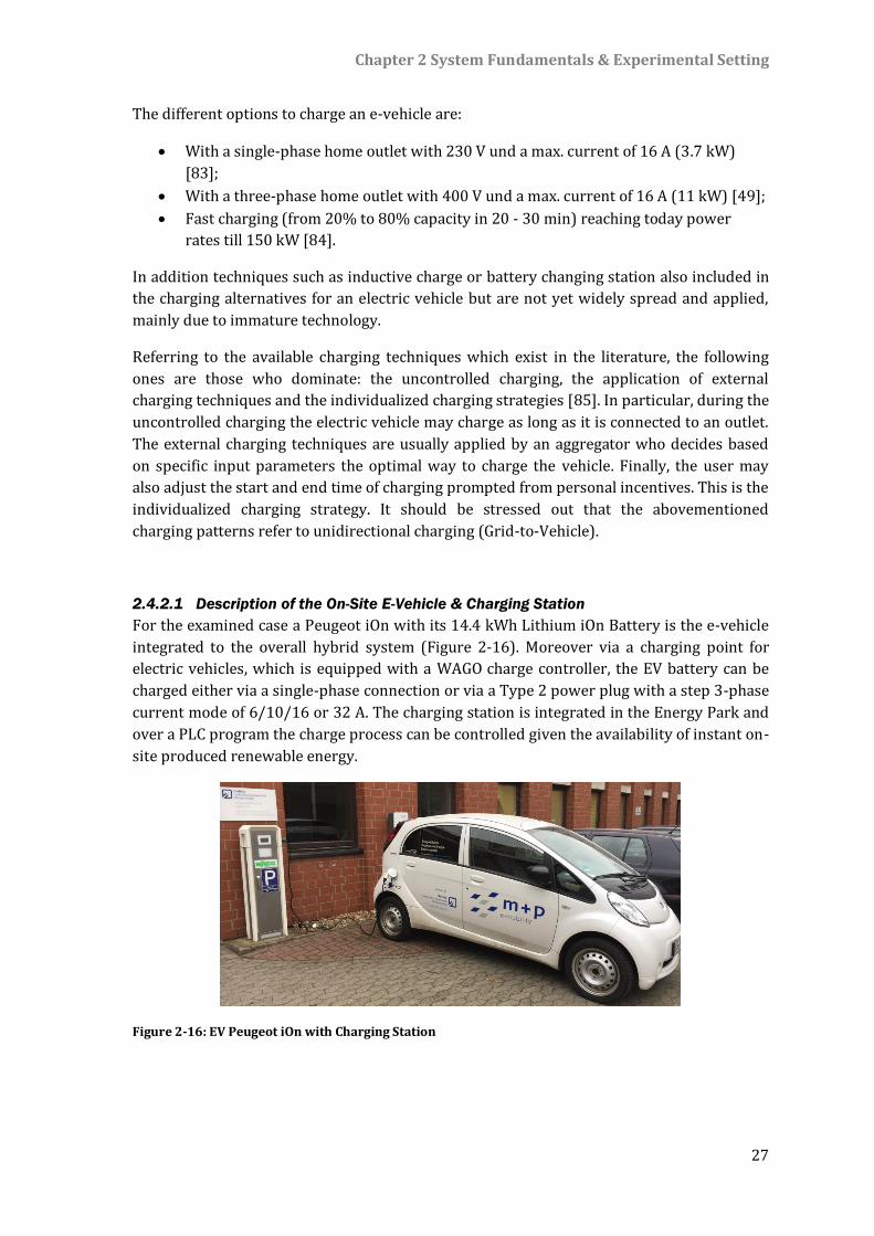
Chapter 2 System Fundamentals & Experimental Setting
27
The different options to charge an e-vehicle are:
With a single-phase home outlet with 230 V und a max. current of 16 A (3.7 kW)
[83];
With a three-phase home outlet with 400 V und a max. current of 16 A (11 kW) [49];
Fast charging (from 20% to 80% capacity in 20 - 30 min) reaching today power
rates till 150 kW [84].
In addition techniques such as inductive charge or battery changing station also included in
the charging alternatives for an electric vehicle but are not yet widely spread and applied,
mainly due to immature technology.
Referring to the available charging techniques which exist in the literature, the following
ones are those who dominate: the uncontrolled charging, the application of external
charging techniques and the individualized charging strategies [85]. In particular, during the
uncontrolled charging the electric vehicle may charge as long as it is connected to an outlet.
The external charging techniques are usually applied by an aggregator who decides based
on specific input parameters the optimal way to charge the vehicle. Finally, the user may
also adjust the start and end time of charging prompted from personal incentives. This is the
individualized charging strategy. It should be stressed out that the abovementioned
charging patterns refer to unidirectional charging (Grid-to-Vehicle).
2.4.2.1 Description of the On-Site E-Vehicle & Charging Station
For the examined case a Peugeot iOn with its 14.4 kWh Lithium iOn Battery is the e-vehicle
integrated to the overall hybrid system (Figure 2-16). Moreover via a charging point for
electric vehicles, which is equipped with a WAGO charge controller, the EV battery can be
charged either via a single-phase connection or via a Type 2 power plug with a step 3-phase
current mode of 6/10/16 or 32 A. The charging station is integrated in the Energy Park and
over a PLC program the charge process can be controlled given the availability of instant on-
site produced renewable energy.
Figure 2-16: EV Peugeot iOn with Charging Station
Chapter 2 System Fundamentals & Experimental Setting
28
2.4.2.2 Modeling of E-Vehicle Load Demand
Based on the three charging patterns previously described (Section 2.4.2), various charging
modes have been designed and developed. Indicatively, Darabi et al. [86] used
transportation data to produce charging load curves based on American driving profiles.
Fernández et al. examine the penetration of EV in an urban area with regard to the
expansion of the local distribution network while Lee et al. focus on creating probabilistic
driving cycles for estimating the impact of the charging process on the grid [87-88].
Westermann et al. have developed an averaged model which stems from measured load
profiles, based on fleet data from fifty electric vehicles [89]. Due to the fact though that the
consumed energy could not be correlated and subsequently predicted, a generalized model
which could be used for individual trips was not feasible. Moreover great emphasis is given
on the impacts of the EV load profile on the distribution grid [90-92] but the effect after the
integration of the charging process of an EV on the house load profile is not widely
discussed or described in the literature.
As in the current study emphasis is given on a residence in Germany and a microscopic
examination is entrenched in a hybrid house installation, an analogous driving cycle should
also be considered. Reports based on charging profiles from other countries can
unfortunately not be utilizable since there is a differentiation in driving behavior among
countries. According to the VDE Studie Elektrofahrzeuge [93] the mean daily vehicle
distance travelled in Germany for a passenger car is approximately 60km. Considering this
parameter as a basic variable of defining a charging profile of an EV, a naturalistic driving
combined cycle of 60km was decided to be performed given that the EV was fully charged at
the beginning of the trip and the charging process was registered. Although such a charging
profile is considered static it has the advantage that is customized to the German driving
behavior and represents the mean passenger. Based on the hypothesis that the driver
always charges at home and the trip end-time is at 19:00 daily, the specific charging method
can be assigned to the uncontrolled charging strategies. Finally another fact which
advocated the adoption of such a charging method is the lack of time-based utility pricing
(or dynamic pricing) from the German grid operators, setting an uncontrolled charging
technique as favorable.
Chapter 3 Hybrid Energy Storage System
29
3 Hybrid Energy Storage System In the previous chapter a thorough literature review in batteries and PV installations used in
the domestic field was conducted. It is scope of this chapter to present the thematic around
the hybrid energy storage system (HESS), which is actually a combination of the two
different types of facilities already described. The examined HESS with its individual
components will be presented and the problematic which arises is going to be analyzed. In
this context the scope of this work is concretized. After a presentation of the existing HESS
control methods it is justified why the Markov Decision Process (MDP) was the selected
applied technique to control the given system. Finally the research questions and the
challenges which were faced during the design of the optimization strategy are addressed
and the limitations of scope are clarified.
3.1 Introduction to Hybrid Energy Storage System (HESS)
The rapid penetration of decentralized energy systems in the energy market during the last
decade and the encouragement to increase the share of self-energy consumption have set
the adoption of storing ideas as substantial in the domestic field. The deployment of one
storage device to gather the surplus of the renewable energy and redirect it to the loads
when a deficit in power occurs is already a standard tactic nowadays. The operation
simplicity of such a system makes it particularly attractive. However, it is common
knowledge that none of the existing storage techniques or battery types for domestic
purposes is optimal for use under any conditions. There are systems whose technology is
already mature but they still lack in other characteristics such as the degradation, the
energy density or the self-discharge. On the contrary, systems with better attributes in cycle
life-time and energy density may underperform in reaction time or in system efficiency.
HESSs are considered optimal to give a solution to such inadequacies since they combine
two (or more) different storage types and consequently they combine also the advantages of
them. They are designed to take advantage from the best of two or more worlds, so as to
exploit and use the positive aspects of each one of the applied stationary storage systems.
The adaptation of a storage system combination is a challenging and highly promising
approach from which a stand-alone installation or a grid-connected system may profit if the
different storage systems are managed to be controlled in an optimal way so as to benefit
from the advantages of the heterogeneous technologies.
Already discussed HESS applications in the literature include among others [94]:
HESSs for hybrid and plug-in vehicles;
HESSs for large scale installations;
HESSs for stand-alone installations in remoted areas;
HESSs for grid connected systems targeting to lower interaction with the Electrical
Power Distribution System.
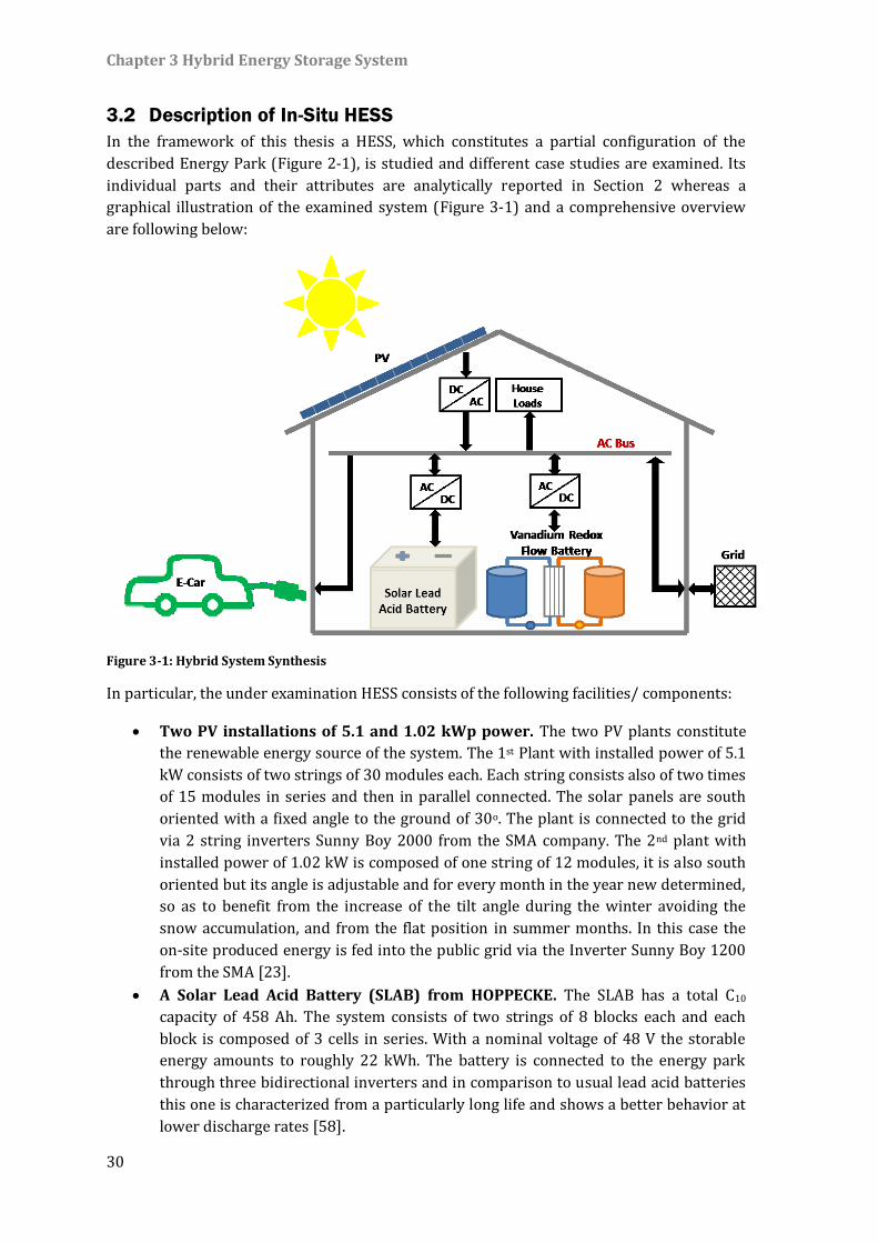
Chapter 3 Hybrid Energy Storage System
30
3.2 Description of In-Situ HESS
In the framework of this thesis a HESS, which constitutes a partial configuration of the
described Energy Park (Figure 2-1), is studied and different case studies are examined. Its
individual parts and their attributes are analytically reported in Section 2 whereas a
graphical illustration of the examined system (Figure 3-1) and a comprehensive overview
are following below:
Figure 3-1: Hybrid System Synthesis
In particular, the under examination HESS consists of the following facilities/ components:
Two PV installations of 5.1 and 1.02 kWp power. The two PV plants constitute
the renewable energy source of the system. The 1st Plant with installed power of 5.1
kW consists of two strings of 30 modules each. Each string consists also of two times
of 15 modules in series and then in parallel connected. The solar panels are south
oriented with a fixed angle to the ground of 30o. The plant is connected to the grid
via 2 string inverters Sunny Boy 2000 from the SMA company. The 2nd plant with
installed power of 1.02 kW is composed of one string of 12 modules, it is also south
oriented but its angle is adjustable and for every month in the year new determined,
so as to benefit from the increase of the tilt angle during the winter avoiding the
snow accumulation, and from the flat position in summer months. In this case the
on-site produced energy is fed into the public grid via the Inverter Sunny Boy 1200
from the SMA [23].
A Solar Lead Acid Battery (SLAB) from HOPPECKE. The SLAB has a total C10
capacity of 458 Ah. The system consists of two strings of 8 blocks each and each
block is composed of 3 cells in series. With a nominal voltage of 48 V the storable
energy amounts to roughly 22 kWh. The battery is connected to the energy park
through three bidirectional inverters and in comparison to usual lead acid batteries
this one is characterized from a particularly long life and shows a better behavior at
lower discharge rates [58].

Chapter 3 Hybrid Energy Storage System
31
A vanadium redox-flow-battery (VRB) system from Prudent Energy™. The VRB
has a storable electric energy of approximately 20 kWh. The liquid electrolyte of
sulphuric acid solution, which amounts to 1,800l, is stored in two tanks and contains
vanadium at different oxidation states. During charging or discharging process the
liquid is pumped to the cell stack, which is composed of 36 single cells, that are
electrically connected in series with nominal voltage equal to 48 V and maximal
current of 130 A and the cell stack is converting chemical energy to electrical and
vice versa [18].
A yearly domestic electric load for a notional single-family house in region of
North-West Germany with four occupants. So as to create a yearly reference load
profile for a single family house with four occupants in a region which belongs to the
“North-West German Lowlands” climate zone the guideline VDI 4655 [81] was taken
into account. Registered data from net meters could also be retrieved and utilised
though it was assessed that the proximity to real data would be at the expense of the
generalisation of the study and of the further exploitation of the results. So a
common used procedure has been adopted in order to facilitate the redimensioning
of the load demand in other cases. So as to determine these reference day load
profiles the following parameters were taken into account:
■ Type of the Building;
■ Climate Zone of the Site of the Building;
■ Number of occupants.
The yearly load demand for charging the Lithium iOn battery of a Peugeot iOn
pure electric vehicle. The Lithium iOn battery has a capacity of 14.4kWh and can
be charged with 10A, 13A or 16A current in flex charge mode and a voltage of
220/230V or 330V when charging in fast mode. To estimate this daily load it was
claimed that the mean vehicle distance travelled each day for a passenger car in
Germany is 60 km [93]. With a fully charged EV and after a real driving combined
cycle of 60 km the charging process of a 14.4 kWh Lithium iOn Battery from the
Peugeot iOn has been registered till its battery was again full and so the yearly load
demand of the E-car was created and aggregated to the yearly domestic electric load,
assuming that the E-vehicle charges always at home.
In the composed scenario the PV plants are considered the energy sources of the system
supported whenever required also by the local grid supply. The vanadium redox flow
battery and the lead acid battery will constitute the stationary storage systems and will be
appropriately utilized to store renewable energy and feed it back to the household
whenever it is required. Finally the electric vehicle and in particular the battery of it as well
as domestic load profiles form the consumer’s behaviour.
3.3 Problem Description & Scope of this Work
Given the abovementioned concept and under the generalized context of energy
management of HESSs in the next sections the overall problem will be defined, the examined
approach will be analyzed, while the boundary conditions and the argumentation round the
selected technique to be applied will be addressed.
Chapter 3 Hybrid Energy Storage System
32
3.3.1 Overall Problem
All HESSs, no matter which topology is deployed, need an additional management system,
which will undertake their control and apply them in a rational sequence with ultimate goal
to increase the total efficiency of the system. Why at all is it such a system necessary? There
are two cases of power allocation that can be applied: either the storage systems share the
amount of power demanded or fed to them, or at each moment only one of them is
prioritized against the other and they operate exclusively interchangeably. In both
described cases it is though substantial to define the external actor which decides in the first
case which proportion of power is ought to be allocated to each facility, and in the second
case which storage system has at the current moment higher priority and should operate as
stand-alone device at this time (i.e. without the support of the other storage facility).
As mentioned in Section 3.1, HESSs are optimally featured with complementary
characteristics and the target of coupling them is to benefit from the strengths of each one.
In a fictional application were two different storage systems are operating alternately the
selection of the most appropriate technique to control the facilities is considered a crucial
matter. Incongruous methods may lead to unadvantageous employment of the storage
systems, resulting in an unprofitable usage of a HESS. Given the specific initial and boundary
conditions and assumptions and the respective selected storage systems which form the
HESS one method outperforms the other or one technique delivers better exploitation of
their attributes. The dynamic energy storage control is responsible for the coordination of
the HESS and the power distribution between the two facilities. Charge and discharge
allocation is undertaken from the control system and the optimal operation solution is
defined.
Referring to the architecture of the HESSs, different types of topologies can be applied to
interlink the storage systems with the rest of the facilities. Direct coupling of the devices
with a single DC converter is a favorable architecture from financial and implementation
aspect; though the constraints in controlling the energy flow make it ineffective. A topology
with a DC-DC converter for each battery and a grid-connected inverter is a better
alternative, increasing the flexibility of the system. Another promising architecture is the
connection of each facility with a DC-AC inverter which introduces higher degree of freedom
in handling the individual components.
3.3.2 Examined Approach
Under the abovementioned context a robust energy management algorithm is to be
developed in the framework of this thesis so as to operate the storage systems, already
described in the Section 3.2, namely the solar lead acid battery and the vanadium redox flow
battery, in the most efficient way in the overall setting consisting of the rest of the facilities.
The utilized storage systems are optimally featured with complementary characteristics and
the target of coupling them is to benefit from the strengths of each one. Having a closer look
to their characteristics, lead acid battery systems are characterized from intolerance at deep
discharges, and short cycle life, especially when high currents occur. Though this is not the
case for the VRB, since such types of batteries are attributed from cycle durability, being
possible to deeply discharge it without damaging the system and they can be easily
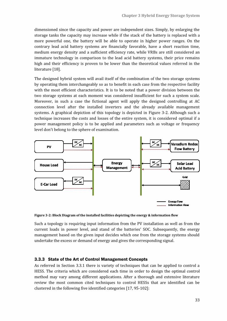
Chapter 3 Hybrid Energy Storage System
33
dimensioned since the capacity and power are independent sizes. Simply, by enlarging the
storage tanks the capacity may increase while if the stack of the battery is replaced with a
more powerful one, the battery will be able to operate in higher power ranges. On the
contrary lead acid battery systems are financially favorable, have a short reaction time,
medium energy density and a sufficient efficiency rate, while VRBs are still considered an
immature technology in comparison to the lead acid battery systems, their price remains
high and their efficiency is proven to be lower than the theoretical values referred in the
literature [18].
The designed hybrid system will avail itself of the combination of the two storage systems
by operating them interchangeably so as to benefit in each case from the respective facility
with the most efficient characteristics. It is to be noted that a power division between the
two storage systems at each moment was considered insufficient for such a system scale.
Moreover, in such a case the fictional agent will apply the designed controlling at AC
connection level after the installed inverters and the already available management
systems. A graphical depiction of this topology is depicted in Figure 3-2. Although such a
technique increases the costs and losses of the entire system, it is considered optimal if a
power management policy is to be applied and parameters such as voltage or frequency
level don’t belong to the sphere of examination.
Figure 3-2: Block Diagram of the installed facilities depicting the energy & information flow
Such a topology is requiring input information from the PV installation as well as from the
current loads in power level, and stand of the batteries’ SOC. Subsequently, the energy
management based on the given input decides which one from the storage systems should
undertake the excess or demand of energy and gives the corresponding signal.
3.3.3 State of the Art of Control Management Concepts
As referred in Section 3.3.1 there is variety of techniques that can be applied to control a
HESS. The criteria which are considered each time in order to design the optimal control
method may vary among different applications. After a thorough and extensive literature
review the most common cited techniques to control HESSs that are identified can be
clustered in the following five identified categories [17, 95-102]:
Chapter 3 Hybrid Energy Storage System
34
Low and High Pass Filters;
Rule-based Algorithms;
Linear Programming Methods;
Reinforcement Learning Techniques;
Hybrid Approaches.
The nature of the considered attributes of the storage systems as well as the type of
evaluation criteria influence the selection of the suitable applied control method. If the
reaction time is the critical decision characteristic then methods based on low- or high-pass
filters are favored [98, 101]. When specific operation boundaries ought to be kept rule
based algorithms are preferred [97, 101, 102] and when these boundaries and the expected
requirements are represented by linear relationships linear programming methods are
applied [96]. If the environment of the controller is deterministic, i.e. the employed models
do not learn from the action evolution, and the degree of freedom during parametrization is
also significant for the developed optimization technique, while a sequential decision-
making problem is to be solved, a decision making algorithm which does not factor in the
preceding states is ideal [17]. Finally hybrid methods are employed when a combination of
characteristics should be taken into account [99-100].
Delving into the already reported control systems for HESSs, it is accrued that the different
employed methods are not ideal for optimizing the current studied system. In particular, in
Zhang et al. [97] rule-based algorithms are applied so as to manage the energy flow between
a supercapacitor and a conventional battery. Parameters such as load demand and battery
output current are compared with threshold values and the respective rule is applied.
Takeda et al. in [101] compare the results extracted from applying two of the above-
mentioned methods so as to control a HESS which is constituted from a LAB and a Lithium
ion battery. The amplitude sharing algorithm, which is a rule-based approach, delivers
better results in comparison to the first order filtering. Moreover, Ise et al. in [102] fuzzy
control logic has been applied so as to manage the power allocation between two storage
systems, namely a superconducting magnet and a secondary battery for an energy storage
system with high energy and power density. This control technique, which belongs to the
rule-based algorithms, has the benefit that it is based on a set of rules which are designed
from experts and the most appropriate alternative is selected without requiring extreme
complicated mathematical knowledge. However, the configuration is becoming extremely
difficult if the system is quite complex [95]. Under the given conditions, the attribution and
setting of a group of rules in advance during the design of the management method for the
examined HESS is considered rather demanding and puzzling, so such a method is not
preferred in the frame of this thesis.
In the literature, the most widely used technique to manage HESSs is the first-order filtering
method. According to it, the high power fluctuations are allocated to one storage system,
often a supercapacitor, and the rest is undertaken from a conventional battery system [98,
99]. This linear filtering is actually designed based on the response time of the two storage
technologies; nonetheless various other parameters are not being considered. Filtering
methods as the ones applied from Li et al. and Takeda et al. [98, 101] are regarded also
unsuitable for system cases as the one described in the current study, since the response
time of the storage systems is not the determinant factor for designing the present
Chapter 3 Hybrid Energy Storage System
35
management system. Such technique is preferable when for instance a supercapacitor is
integrated in the HESS and in both previously referred cases such a device is part of the
examined system.
Another HESS is also studied from Nikolai et al. [96], referring to the project on the island
Pellworm of the North Sea. By exploiting all the renewable energy sources installed on it (a
PV park of 700kWp and a wind farm of 300kWp) and with the support of several storage
systems (mainly lithium-ion batteries and redox flow batteries) a stable and cost-effective
energy supply is pursued. In this case a mixed integer linear programming method is
applied for the optimization approach. While linear programming algorithms are easily
comprehensive and simply applicable, though they lack in the generalization part, and
therefore avoided if a global solution is claimed, as in the examined case.
Hybrid methods are recommended because they combine different techniques and they are
often preferred in the literature. For instance, Abbey et al. in [100] apply a low-pass filter
combined with two neural networks decide the percentage of the reference power which
should be allocated to each facility. Such a technique is though unfavourable because the
partitioning of the demanded energy or the surplus of the on-site generation between the
existing two storage devices which constitute the examined HESS could worsen their
efficiency behavior. Moreover, as already explained earlier, low pass filters do not apply in a
case as the one designed here. For this reason, the combination of a rule based algorithm
with a filtering technique, as the one conceptualized from Li et al. in [99], still cannot fulfill
the needs addressed from this topic.
Conclusively, as it is argued in [100], it is concluded that an ideal energy management
system which can be applied in any case cannot be nominated, since every application of
hybrid energy storage systems is attributed from varying characteristics, which must be
taken into account during the design of the control process and the optimization goal or
parameter can be different in each case. However, advanced control algorithms which are
optimized-based are considered as more efficient in acquiring better results. It is also to be
noted, that the selection of the appropriate technique to manage the energy flow in the HESS
is considered crucial when an optimized solution is sought and case specific solution is in
most cases addressed.
3.3.4 Beyond the State of the Art
The designed platform under the examined concept is deterministic, because the respective
models which represent the individual components of the system are validated and
correspond to the real applied facilities which exist in the Hybrid Renewable Energy Park of
the Ostfalia University in Wolfenbüttel. In addition, the adopted models do not include a
learning process, i.e. for the same inputs values and under the same conditions the extracted
output remains always the same. Finally, the ageing process of the stationary storage
systems or other intermittent parameters do not intrude in the design process so as to
modify the already formed environment and affect the output values. Based on these
prerequisites it is decided that the optimal controlling of the existing HESSs can be
accomplished using the Markov Decision Process.
Chapter 3 Hybrid Energy Storage System
36
MDP is considered a mathematical framework to support the decision making. The decision
maker (agent) after taking into account the rewards (which are calculated each moment
based on the efficiency grade and the state of charge of the two stationary storage systems)
is favoring one action and subsequently one battery system against the other. The ultimate
target from applying this process is to optimize the alternate modus of the storage systems
by operating them under high-efficiency conditions in the long-term. Such a technique is
appropriate in cases where the next time step action is exclusively dependent on the current
states of the system (i.e. the SOC of the storage systems and the required/ abundant power)
while the precise calculation of these variables is considered determinant for the correct
design of the MDP. In this study, the use of validated and verified models guarantees the
systematic approach that is chosen.
Such a method is applied to solve several energy allocation problems. Jimenez in [16]
applies an MDP to succeed resource allocation and load shedding in a system consisting of a
decentralized energy source, one storage system and loads. Zhou et al. in [103] conclude
that an MDP applied in a system composed of a wind farm, a storage facility and a
transmission line to the grid, delivers 15% better results in comparison to a Naive policy. A
similar system with the one referred from Zhou et al. [103] has been studied from Murtaza
and Tahir in [104], with an ultimate target to minimize the data transmission level and keep
the battery energy between specified levels, though in this case renewable energy
generation stems from not from wind but from PV facilities. Moreover, in the study of Xu et
al. [105] the MDP is applied in a load-serving entity having as evaluation criterion the
decrease of energy costs. Grillo et al. have applied a control policy, based again on the theory
of MDP, though in this case the scheduling refers to a test network in medium voltage (MV)
level. The authors tried not only to minimize the cost of energy but also to reduce the
network losses [106].
Qiu in [17] studies a HESS in microgrid operation. It is composed of a LAB, a VRB and target
of the study is to minimize the system losses, via controlling the storage devices with an
MDP. Although the stationary storage systems are of the same type as the ones examined in
the framework of this thesis and the applied control technique is the MDP, there are several
design points and physical characteristics that differentiate substantially the
abovementioned study with the current one. Specifically, for simplicity and dimensionality
reasons much fewer states are selected during the design of the MDP as the ones predefined
under the current study in Section 5.2. Another differentiation point is the level of
accomplished generalization. In particular, although the applied method was developed for
the already described HESS, scope of this work was also to design a technique that can be
generalized for every other similar HESS simply by respectively parametrizing the
analogous sections in the designed process, given equivalent boundary conditions. This part
is however not succeeded from Qiu in [17] due to physical constraints of the storage
systems. A more detailed description of this argumentation is provided in Section 5.2.
Furthermore, in the discussed study a power distribution via a DC bus is the selected
topology while in the examined case the components are connected over an AC bus. Last but
not least, the overall target in each study is heterogeneous. In the abovementioned system
losses should be ultimately minimized whereas scope of this work is to maximize the
consumption of the on-site renewable energy by covering the local demand and to minimize
Chapter 3 Hybrid Energy Storage System
37
the power interaction between the fictional building and the grid, as described in Section
3.3.4.
Concluding from the abovementioned, the current study differentiates from other similar
ones in the design and modelling of the individual devices as well as the interactions among
them which depict precisely the reality. The systems are designed considering their
functional specifications and no simplified version of models has been used. Moreover, all
energy losses are taken into account when modelling each facility as well as when the
interconnections among them were captured and represented at the design of the entire
system. It is also to be noted that in many studies the coordination of the systems is
undertaken from an external actor. In the framework of this thesis the management is
implemented from the local controller of the decentralized platform showing that individual
solutions contribute to relieve the strain of the grid from peak power and increase the self-
energy consumption grade of the residence. Although as abovementioned, HESSs which are
utilized to store abundant PV energy and reallocate it back to existing loads are already
registered in the literature, the management of a hybrid system which consists of a VRB,
which operates as a mid-term storage system and a LAB, which is considered a short-term
equivalent, in combination with the fluctuating and occasionally acute load demand due to
the charging process of a pure E-Vehicle has not yet been studied. In addition, VRB systems
applications in the residential sector are barely mentioned in the literature [107]. In
addition, in the described HESS each PV plant as well as storage device is equipped with a
respective DC-AC inverter and the facilities maintain their own internal energy management
system. It should be also noted that the HESS operates in grid-connected mode, so when a
surplus or shortage of power occurs the grid accommodates each case.
3.3.5 Evaluation Criteria
So as to evaluate the applied technique a benchmark method was also implemented,
according to which priority in charging and discharging was always given to the battery
system with the higher efficiency grade on the examined time slot. This naive approach is
considered a heuristic tactic and the evaluation criteria, according to which the two policies
were assessed, are two energy indexes, i.e. supply cover factor and the grid interaction index
which are described from the following equations [108]:
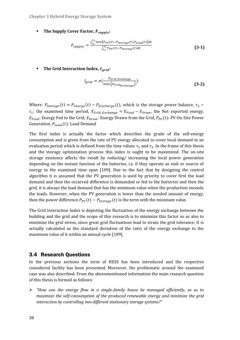
Chapter 3 Hybrid Energy Storage System
38
The Supply Cover Factor, 𝑭𝒔𝒖𝒑𝒑𝒍𝒚:
𝐹𝑠𝑢𝑝𝑝𝑙𝑦 =∫ 𝑚𝑖𝑛[𝑃𝑃𝑉(𝑡)−𝑃𝑆𝑡𝑜𝑟𝑎𝑔𝑒(𝑡),𝑃𝐿𝑜𝑎𝑑(𝑡)]𝑑𝑡𝜏2𝜏1
∫ 𝑃𝑃𝑉(𝑡)−𝑃𝑆𝑡𝑜𝑟𝑎𝑔𝑒(𝑡)𝑑𝑡𝜏2𝜏1
(3-1)
The Grid Interaction Index, 𝑰𝒈𝒓𝒊𝒅:
𝐼𝑔𝑟𝑖𝑑 = 𝜎(𝐸𝐺𝑟𝑖𝑑_𝐸𝑥𝑐ℎ𝑎𝑛𝑔𝑒
max(|𝐸𝐺𝑟𝑖𝑑𝐸𝑥𝑐ℎ𝑎𝑛𝑔𝑒 |))
(3-2)
Where: 𝑃𝑆𝑡𝑜𝑟𝑎𝑔𝑒(𝑡) = 𝑃𝐶ℎ𝑎𝑟𝑔𝑒(𝑡) − 𝑃𝐷𝑖𝑠𝑐ℎ𝑎𝑟𝑔𝑒(𝑡), which is the storage power balance, 𝜏2 −
𝜏1: the examined time period, 𝐸𝐺𝑟𝑖𝑑_𝐸𝑥𝑐ℎ𝑎𝑛𝑔𝑒 = 𝐸𝐹𝑒𝑒𝑑 − 𝐸𝐷𝑟𝑎𝑤, the Net exported energy,
𝐸𝐹𝑒𝑒𝑑: Energy Fed to the Grid, 𝐸𝐷𝑟𝑎𝑤: Energy Drawn from the Grid, 𝑃𝑃𝑉(𝑡): PV On-Site Power
Generation, 𝑃𝐿𝑜𝑎𝑑(𝑡): Load Demand
The first index is actually the factor which describes the grade of the self-energy
consumption and is given from the rate of PV energy allocated to cover local demand in an
evaluation period which is defined from the time values 𝜏1 and 𝜏2. In the frame of this thesis
and the storage optimization process this index is ought to be maximized. The on-site
storage existence affects the result by reducing/ increasing the local power generation
depending on the instant function of the batteries, i.e. if they operate as sink or source of
energy in the examined time span [109]. Due to the fact that by designing the control
algorithm it is assumed that the PV generation is used by priority to cover first the load
demand and then the occurred difference is demanded or fed to the batteries and then the
grid, it is always the load demand that has the minimum value when the production exceeds
the loads. However, when the PV generation is lower than the needed amount of energy,
then the power difference 𝑃𝑃𝑉(𝑡) − 𝑃𝑆𝑡𝑜𝑟𝑎𝑔𝑒(𝑡) is the term with the minimum value.
The Grid Interaction Index is depicting the fluctuation of the energy exchange between the
building and the grid and the scope of this research is to minimize this factor so as also to
minimize the grid stress, since great grid fluctuations lead to strain the grid tolerance. It is
actually calculated as the standard deviation of the ratio of the energy exchange to the
maximum value of it within an annual cycle [109].
3.4 Research Questions
In the previous sections the term of HESS has been introduced and the respective
considered facility has been presented. Moreover, the problematic around the examined
case was also described. From the abovementioned information the main research question
of this thesis is formed as follows:
“How can the energy flow in a single-family house be managed efficiently, so as to
maximize the self-consumption of the produced renewable energy and minimize the grid
interaction by controlling two different stationary storage systems?”
Chapter 3 Hybrid Energy Storage System
39
Solution Approach: After defining the overall concept and the boundary conditions of the
studied case, each facility is modelled in MATLAB® / Simulink® environment and after
precisely representing the interactions among the designed blocks, an energy management
policy is applied, which will undertake the role of the “decision-maker” and will mandate the
storage systems by triggering them when a surplus or a demand of power is occurring,
according to their SOC as well as their efficiency grade and power level.
Several sub questions emanate from the main research problem, which is previously
described. These are formulated as follows:
“Which are the appropriate models to represent the existing facilities?”
“Which method is optimal to be applied in order to implement the selected energy
management policy so as to control the charging and discharging process of two
stationary storage systems?”
“How can the chosen technique be evaluated?”
Solution Approach: After specifying the examined environment by identifying and
developing the most suitable models and after creating the charging scenario for the E-
Vehicle based on literature and experimental data, a thorough literature review was
conducted for evaluating the possible methods that can be applied to control the given HESS
and the most appropriate was selected. Finally, a benchmark method for controlling the
facilities was also provided and analyzed and the results from the two case studies were
compared, based on the evaluation criteria presented in Section 3.3.4.
3.5 Limitations of Scope & Challenges
Due to the fact that the design of the control algorithm requires the exact knowledge of the
remaining stored energy, it was quite challenging to model the existing facilities by applying
common used techniques, which represent the physical fundamentals and principles of each
facility, and simultaneously taking into account the explicit specifications of the respective
module. The validation and verification of the designed models contributed towards the
correct representation of them. For this reason the modelling part occupies a substantial
part of the current thesis and the applied methods are discussed in detail in the following
chapter (Section 4).
In addition, the randomness in the weather conditions in the central north region of
Germany forms a highly fluctuating PV production profile. The intermittency of the power
generation was another challenge to be faced when planning the management policy,
because the great fluctuation in the current shortage or surplus of energy demanded a
robust algorithm which could manage these situations. In finite state-action problems, as
the one tackled in the frame of this thesis, if the system model would be running in minute-
step intervals, the application of the 𝑄-Learning algorithm to solve the MDP optimization
problem would cause slow convergence to the optimal action-value function. It was thus
decided to work in hour-step intervals, trying to reduce the complexity of the applied
algorithm by making a compromise between accuracy and convergence. An alternative
would be the application of the speedy 𝑄-Learning algorithm as implemented from [110].

Chapter 3 Hybrid Energy Storage System
40
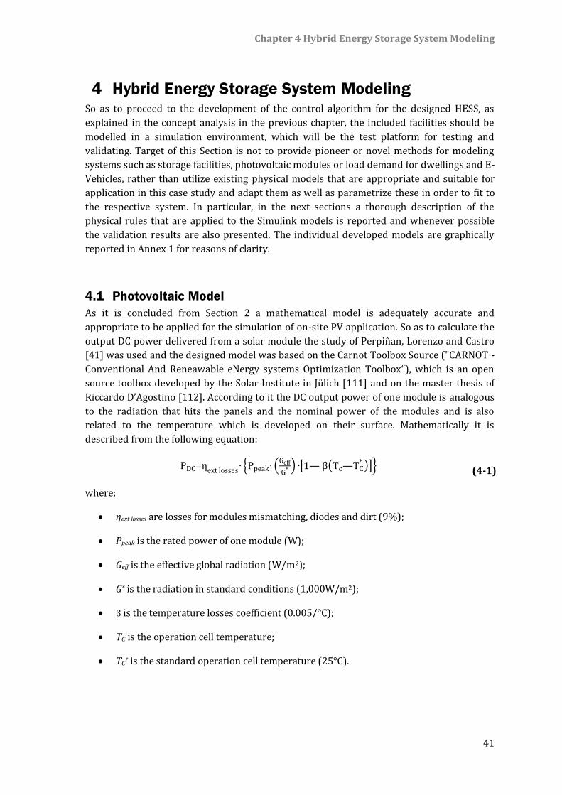
Chapter 4 Hybrid Energy Storage System Modeling
41
4 Hybrid Energy Storage System Modeling So as to proceed to the development of the control algorithm for the designed HESS, as
explained in the concept analysis in the previous chapter, the included facilities should be
modelled in a simulation environment, which will be the test platform for testing and
validating. Target of this Section is not to provide pioneer or novel methods for modeling
systems such as storage facilities, photovoltaic modules or load demand for dwellings and E-
Vehicles, rather than utilize existing physical models that are appropriate and suitable for
application in this case study and adapt them as well as parametrize these in order to fit to
the respective system. In particular, in the next sections a thorough description of the
physical rules that are applied to the Simulink models is reported and whenever possible
the validation results are also presented. The individual developed models are graphically
reported in Annex 1 for reasons of clarity.
4.1 Photovoltaic Model
As it is concluded from Section 2 a mathematical model is adequately accurate and
appropriate to be applied for the simulation of on-site PV application. So as to calculate the
output DC power delivered from a solar module the study of Perpiñan, Lorenzo and Castro
[41] was used and the designed model was based on the Carnot Toolbox Source ("CARNOT -
Conventional And Reneawable eNergy systems Optimization Toolbox“), which is an open
source toolbox developed by the Solar Institute in Jülich [111] and on the master thesis of
Riccardo D’Agostino [112]. According to it the DC output power of one module is analogous
to the radiation that hits the panels and the nominal power of the modules and is also
related to the temperature which is developed on their surface. Mathematically it is
described from the following equation:
PDC=ηext losses
∙ {Ppeak∙ (Geff
G* ) ∙[1— β(Tc—TC* )]} (4-1)
where:
ηext losses are losses for modules mismatching, diodes and dirt (9%);
Ppeak is the rated power of one module (W);
Geff is the effective global radiation (W/m2);
G* is the radiation in standard conditions (1,000W/m2);
β is the temperature losses coefficient (0.005/°C);
TC is the operation cell temperature;
TC* is the standard operation cell temperature (25°C).
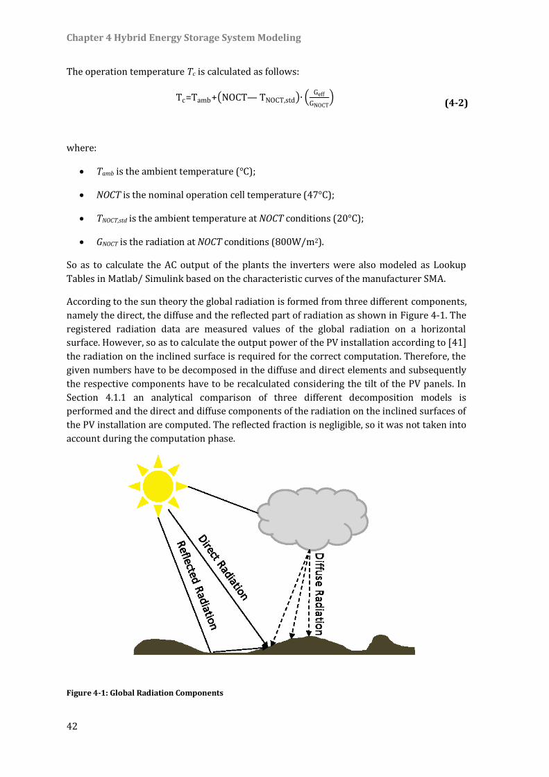
Chapter 4 Hybrid Energy Storage System Modeling
42
The operation temperature Tc is calculated as follows:
Tc=Tamb+(NOCT— TNOCT,std)∙ (Geff
GNOCT)
(4-2)
where:
Tamb is the ambient temperature (°C);
NOCT is the nominal operation cell temperature (47°C);
TNOCT,std is the ambient temperature at NOCT conditions (20°C);
GNOCT is the radiation at NOCT conditions (800W/m2).
So as to calculate the AC output of the plants the inverters were also modeled as Lookup
Tables in Matlab/ Simulink based on the characteristic curves of the manufacturer SMA.
According to the sun theory the global radiation is formed from three different components,
namely the direct, the diffuse and the reflected part of radiation as shown in Figure 4-1. The
registered radiation data are measured values of the global radiation on a horizontal
surface. However, so as to calculate the output power of the PV installation according to [41]
the radiation on the inclined surface is required for the correct computation. Therefore, the
given numbers have to be decomposed in the diffuse and direct elements and subsequently
the respective components have to be recalculated considering the tilt of the PV panels. In
Section 4.1.1 an analytical comparison of three different decomposition models is
performed and the direct and diffuse components of the radiation on the inclined surfaces of
the PV installation are computed. The reflected fraction is negligible, so it was not taken into
account during the computation phase.
Figure 4-1: Global Radiation Components
Chapter 4 Hybrid Energy Storage System Modeling
43
For the calculation of the effective global radiation Geff, i.e. the global radiation on the
inclined surface of the solar panels, the sun azimuth and altitude had to be specified. In
Figure 4-2 the various angles that appear in the following calculations are graphically
explained. The adopted method for computing these values was based on the DIN 5034
Norm [113]. According to it the parameter J' as well as the solar declination δ(J'), which
represents the angle that is formed if a direct line is drawn from the center of the sun to
center of the earth and the equatorial plane, and the time equation 𝑇𝑒𝑞 are calculated as
follows:
J'=360o·Day of the Year
Total Number of Days in a Year
(4-3)
δ(J')={0.3948—23.2559· cos (J'+9.1o)—
0.3915* cos (2·J'+5.4o)— 0.1764· cos (3·J'+26
o) }o
(4-4)
𝑇𝑒𝑞(J')={0.0066+7.3525· cos (J'+85.9o)+
9.9359· cos (2·J'+108.9o)+0.3387· cos (3·J'+105.2
o) }min
(4-5)
From the Local Time LT, the time zone and the longitude of the region the Local Mean Time
LMT is extracted as given below:
LMT=LT— Time_Zone+4·Longitude·min/° (4-6)
Then the Local Apparent Time LAT and the time angle ω, which is the true solar time and
represents the difference between noon and the local apparent time, are calculated before
completing with the calculation of the sun altitude γs and the azimuth as [114].
LAT=LMT+𝑇𝑒𝑞(J') (4-7)
ω=(12.00h— LAT)·15o/h (4-8)
Finally the Sun Altitude γs and the azimuth as are extracted from the calculated time angle
ω, the solar declination δ and the local Latitude φ:
Chapter 4 Hybrid Energy Storage System Modeling
44
γs=arcsin (cosω·cosφ· cos δ +sinφ· sin δ ) (4-9)
where:
𝜑 is the local Latitude.
Azimuth: as={180o— arccos
sinγs·sinφ- sin δ
cosγs·cosφfor LAT≤12:00h
180o + arccossinγs·sinφ- sin δ
cosγs·cosφ for LAT>12:00h
(4-10)
Figure 4-2: Solar incidence angle on a PV panel
Given the sun altitude and azimuth the diffuse and the direct components of the global
radiation on a horizontal surface are calculated based on the model developed from Reindl
et al. [115-116]. The decomposition of the global radiation is essential for the further
calculations of the diffuse and direct parts of the radiation reaching the inclined panel. The
clearness index kT (ratio of hourly global horizontal to hourly extraterrestrial radiation)
[115] and the solar zenith angle γs are the variables which determine the diffuse fraction of
the global solar irradiation.
According to that:
kT= EGlobal,hor
Eo·sinγs
(4-11)
where:
Eois the extraterrestrial irradiance (solar constant) equal to 1360.8 W/m2
EDiffuse,hor={
EGlobal,hor·(1.020 — 0.254·kT+0.0123·sinγs), for kT≤0.3
EGlobal,hor · (1.400 — 1.749 · kT + 0.177 · sinγs) , for 0.3 < kT < 0.78
EGlobal,hor · (0.486 · kT— 0.182 · sinγs), for kT ≥ 0.78
(4-12)
Chapter 4 Hybrid Energy Storage System Modeling
45
Finally the direct fraction is extracted from the deduction of the diffuse part from the global
radiation on the horizontal surface and is mathematically expressed from the following
equation:
EDirect,hor=EGlobal,hor— EDiffuse,hor (4-13)
4.1.1 Decomposition Models
Having already assessed the direct and diffuse components of the global irradiance on the
horizontal plane, the calculation of the diffuse fraction of the irradiance on the inclined
surface follows. Three different computation models are applied and their accuracy is
estimated. These are namely the isotropic sky model of Liu and Jordan [117], the Klucher
model [118] and the Perez et al. model [119-121], and their respective equations are given
below [122]:
Isotropic Sky Model A.
EDiffuse,gen=EDiffuse,hor·1
2·(1+cosγE)
(4-14)
where:
γE is the slope angle of the module.
In the isotropic approach it is assumed that the radiation is always the same, regardless the
sky direction, which is interpreted as the beam density is uniformly distributed [114]. This
model is preferred for rough estimates or when the sky is overcast. Generally though
anisotropic models are more appropriate for calculating the diffuse part of the irradiance on
inclined surface since the irradiance density differs greatly according to the direction of the
sky. Klucher and Perez model which are next described belong to this cluster [114].
Klucher Model B.
EDiffuse,gen=EDiffuse,hor·1
2·(1+cosγE
)· (1+F· (sinγE
2)
3) ·(1+F·(cosθgen)2·(cosγs)3) (4-15)
The factor F is given by:
F= 1— (EDiffuse,hor
EGlobal,hor)
2 (4-16)
The incidence angle θgen between the sun direction and the normal vector n perpendicular
to the tilted surface can be calculated as:

Chapter 4 Hybrid Energy Storage System Modeling
46
θgen=arccos (— cosγs· sin γE · cos(as–aE)+sinγs·cosγE) (4-17)
where:
aE is the azimuth angle of the module.
Perez Model C.
The calculation of the diffuse radiation according to Perez model is requiring more effort
[123] and the steps followed are shown below. First the Air Mass index AM, the sky Clarity
Index ε and the brightness Index Δ are calculated according to the following equations:
Air Mass: AM=1
sinγs
(4-18)
Sky Clarity Index: ε=
EDiffuse,hor+EDirect,hor· sin-1 γs
EDiffuse,hor+κ·θhor
3
1+κ·θhor3 (4-19)
Brightness Index: Δ=AM·EDiffuse,hor
E0
(4-20)
where:
θhor is the angle of incidence of the sunlight, expressed in rad.
The Air Mass coefficient describes the path length that the light follows through the
atmosphere normalized to the shortest path it could take. Sky Clarity Index is actually
depicting the pollution in the air and mixes the parts of background diffuse irradiance and
the circumsolar part. Variations of Δ show actually the opacity/thickness of the clouds [120,
124].
The circumsolar and horizon brightness coefficients F1 and F2 respectively can be expressed
as:
F1=F11(ε)+F12(ε)·Δ+F13(ε)·θhor (4-21)
F2=F21(ε)+F22(ε)·Δ+F23(ε)·θhor (4-22)
where:
F11(ε), F12(ε), F13(ε), F21(ε), F22(ε), F23(ε) are constants stemming from the Table 4-1
[114]. The Table is formed based on eight consecutive ε-classes which correspond to
eight sky-clearness indices ε-ranges.
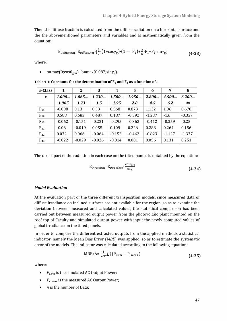
Chapter 4 Hybrid Energy Storage System Modeling
47
Then the diffuse fraction is calculated from the diffuse radiation on a horizintal surface and
the the abovementioned parameters and variables and is mathematically given from the
equation:
EDiffuse,gen=EDiffuse,hor·[1
2·(1+cosγE
)·(1 — F1)+a
b·F1+F2·sinγE] (4-23)
where:
α=max (0;cosθgen) , b=max (0.087;sinγs).
Table 4-1: Constants for the determination of F1 and F2 as a function of ε
ε-Class 1 2 3 4 5 6 7 8
ε 1.000… 1.065… 1.230… 1.500… 1.950… 2.800… 4.500… 6.200…
1.065 1.23 1.5 1.95 2.8 4.5 6.2 ∞
F11 -0.008 0.13 0.33 0.568 0.873 1.132 1.06 0.678
F12 0.588 0.683 0.487 0.187 -0.392 -1.237 -1.6 -0.327
F13 -0.062 -0.151 -0.221 -0.295 -0.362 -0.412 -0.359 -0.25
F21 -0.06 -0.019 0.055 0.109 0.226 0.288 0.264 0.156
F22 0.072 0.066 -0.064 -0.152 -0.462 -0.823 -1.127 -1.377
F23 -0.022 -0.029 -0.026 -0.014 0.001 0.056 0.131 0.251
The direct part of the radiation in each case on the tilted panels is obtained by the equation:
EDirect,gen=EDirect,hor·cosθgen
sinγs
(4-24)
Model Evaluation
At the evaluation part of the three different transposition models, since measured data of
diffuse irradiance on inclined surfaces are not available for the region, so as to examine the
deviation between measured and calculated values, the statistical comparison has been
carried out between measured output power from the photovoltaic plant mounted on the
roof top of Faculty and simulated output power with input the newly computed values of
global irradiance on the tilted panels.
In order to compare the different extracted outputs from the applied methods a statistical
indicator, namely the Mean Bias Error (MBE) was applied, so as to estimate the systematic
error of the models. The indicator was calculated according to the following equation:
MBE/A= 1
n*P̅∑ (Pi,sim— Pi.meas
n1 ) (4-25)
where:
Pi,sim is the simulated AC Output Power;
Pi.meas is the measured AC Output Power;
n is the number of Data;
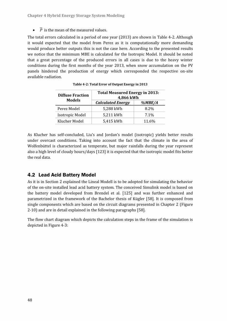
Chapter 4 Hybrid Energy Storage System Modeling
48
P is the mean of the measured values.
The total errors calculated in a period of one year (2013) are shown in Table 4-2. Although
it would expected that the model from Perez as it is computationally more demanding
would produce better outputs this is not the case here. According to the presented results
we notice that the minimum MBE is calculated for the Isotropic Model. It should be noted
that a great percentage of the produced errors in all cases is due to the heavy winter
conditions during the first months of the year 2013, when snow accumulation on the PV
panels hindered the production of energy which corresponded the respective on-site
available radiation.
Table 4-2: Total Error of Output Energy in 2013
Diffuse Fraction Models
Total Measured Energy in 2013: 4,866 kWh
Calculated Energy %MBE/A
Perez Model 5,288 kWh 8.2%
Isotropic Model 5,211 kWh 7.1%
Klucher Model 5,415 kWh 11.6%
As Klucher has self-concluded, Liu’s and Jordan’s model (isotropic) yields better results
under overcast conditions. Taking into account the fact that the climate in the area of
Wolfenbüttel is characterized as temperate, but major rainfalls during the year represent
also a high level of cloudy hours/days [123] it is expected that the isotropic model fits better
the real data.
4.2 Lead Acid Battery Model
As it is in Section 2 explained the Lineal Modell is to be adopted for simulating the behavior
of the on-site installed lead acid battery system. The conceived Simulink model is based on
the battery model developed from Brendel et al. [125] and was further enhanced and
parametrized in the framework of the Bachelor thesis of Kügler [58]. It is composed from
single components which are based on the circuit diagrams presented in Chapter 2 (Figure
2-10) and are in detail explained in the following paragraphs [58].
The flow chart diagram which depicts the calculation steps in the frame of the simulation is
depicted in Figure 4-3:
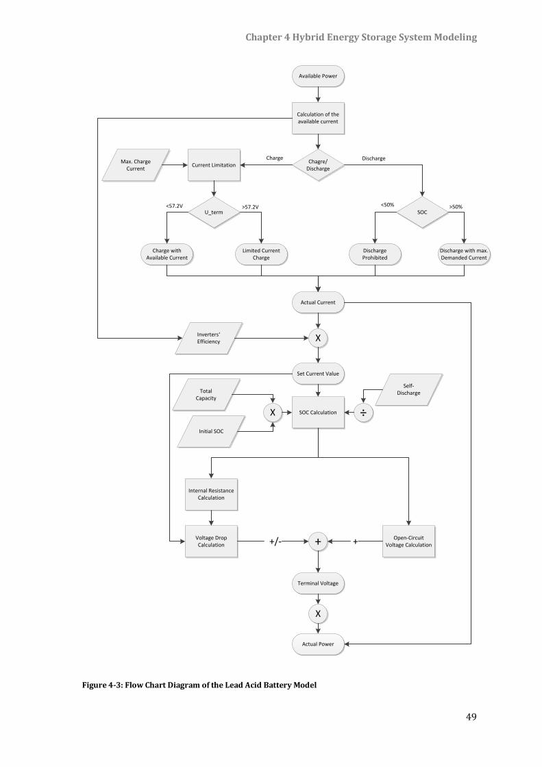
Chapter 4 Hybrid Energy Storage System Modeling
49
Available Power
Calculation of the available current
Chagre/Discharge
Current LimitationMax. Charge
Current
U_term SOC
Charge with Available Current
Limited Current Charge
Discharge Prohibited
Discharge with max. Demanded Current
Actual Current
Inverters‘ Efficiency X
Set Current Value
SOC Calculation ÷ X
Total Capacity
Initial SOC
Self-Discharge
Voltage Drop Calculation
Internal Resistance Calculation
Open-Circuit Voltage Calculation
Terminal Voltage
+
X
Actual Power
+/- +
<50% >50%>57.2V<57.2V
Charge Discharge
Figure 4-3: Flow Chart Diagram of the Lead Acid Battery Model
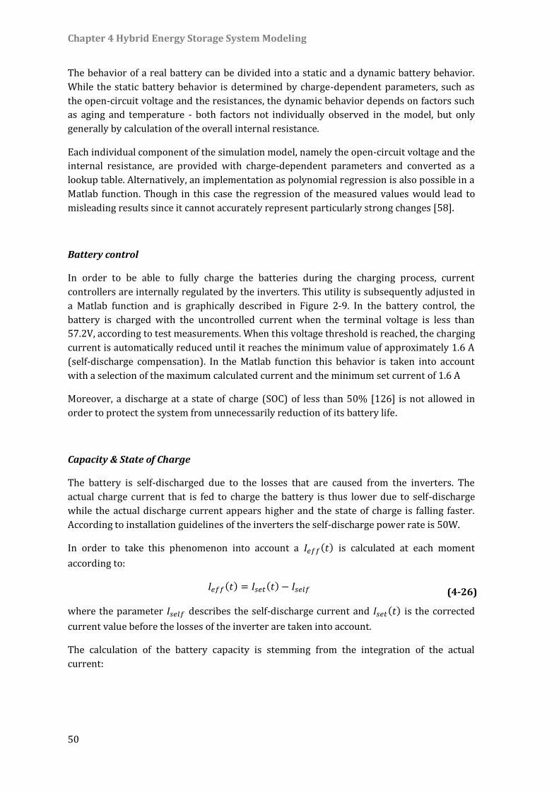
Chapter 4 Hybrid Energy Storage System Modeling
50
The behavior of a real battery can be divided into a static and a dynamic battery behavior.
While the static battery behavior is determined by charge-dependent parameters, such as
the open-circuit voltage and the resistances, the dynamic behavior depends on factors such
as aging and temperature - both factors not individually observed in the model, but only
generally by calculation of the overall internal resistance.
Each individual component of the simulation model, namely the open-circuit voltage and the
internal resistance, are provided with charge-dependent parameters and converted as a
lookup table. Alternatively, an implementation as polynomial regression is also possible in a
Matlab function. Though in this case the regression of the measured values would lead to
misleading results since it cannot accurately represent particularly strong changes [58].
Battery control
In order to be able to fully charge the batteries during the charging process, current
controllers are internally regulated by the inverters. This utility is subsequently adjusted in
a Matlab function and is graphically described in Figure 2-9. In the battery control, the
battery is charged with the uncontrolled current when the terminal voltage is less than
57.2V, according to test measurements. When this voltage threshold is reached, the charging
current is automatically reduced until it reaches the minimum value of approximately 1.6 A
(self-discharge compensation). In the Matlab function this behavior is taken into account
with a selection of the maximum calculated current and the minimum set current of 1.6 A
Moreover, a discharge at a state of charge (SOC) of less than 50% [126] is not allowed in
order to protect the system from unnecessarily reduction of its battery life.
Capacity & State of Charge
The battery is self-discharged due to the losses that are caused from the inverters. The
actual charge current that is fed to charge the battery is thus lower due to self-discharge
while the actual discharge current appears higher and the state of charge is falling faster.
According to installation guidelines of the inverters the self-discharge power rate is 50W.
In order to take this phenomenon into account a 𝐼𝑒𝑓𝑓(𝑡) is calculated at each moment
according to:
𝐼𝑒𝑓𝑓(𝑡) = 𝐼𝑠𝑒𝑡(𝑡) − 𝐼𝑠𝑒𝑙𝑓 (4-26)
where the parameter 𝐼𝑠𝑒𝑙𝑓 describes the self-discharge current and 𝐼𝑠𝑒𝑡(𝑡) is the corrected
current value before the losses of the inverter are taken into account.
The calculation of the battery capacity is stemming from the integration of the actual
current:
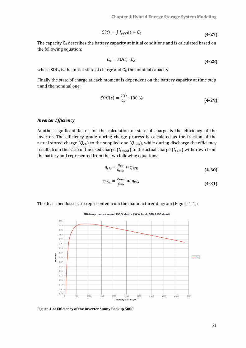
Chapter 4 Hybrid Energy Storage System Modeling
51
𝐶(𝑡) = ∫ 𝐼𝑒𝑓𝑓𝑑𝑡 + 𝐶0 (4-27)
The capacity C0 describes the battery capacity at initial conditions and is calculated based on
the following equation:
𝐶0 = 𝑆𝑂𝐶0 · 𝐶𝑁 (4-28)
where SOC0 is the initial state of charge and CN the nominal capacity.
Finally the state of charge at each moment is dependent on the battery capacity at time step
t and the nominal one:
𝑆𝑂𝐶(𝑡) =𝐶(𝑡)
𝐶𝑁· 100 % (4-29)
Inverter Efficiency
Another significant factor for the calculation of state of charge is the efficiency of the
inverter. The efficiency grade during charge process is calculated as the fraction of the
actual stored charge (𝑄𝑐ℎ) to the supplied one (𝑄𝑠𝑢𝑝), while during discharge the efficiency
results from the ratio of the used charge (𝑄𝑢𝑠𝑒𝑑) to the actual charge (𝑄𝑑𝑖𝑠) withdrawn from
the battery and represented from the two following equations:
𝜂𝑐ℎ =𝑄𝑐ℎ
𝑄𝑠𝑢𝑝≈ 𝜂𝑊𝑅
(4-30)
𝜂𝑑𝑖𝑠 =𝑄𝑢𝑠𝑒𝑑
𝑄𝑑𝑖𝑠≈ 𝜂𝑊𝑅
(4-31)
The described losses are represented from the manufacturer diagram (Figure 4-4):
Figure 4-4: Efficiency of the Inverter Sunny Backup 5000
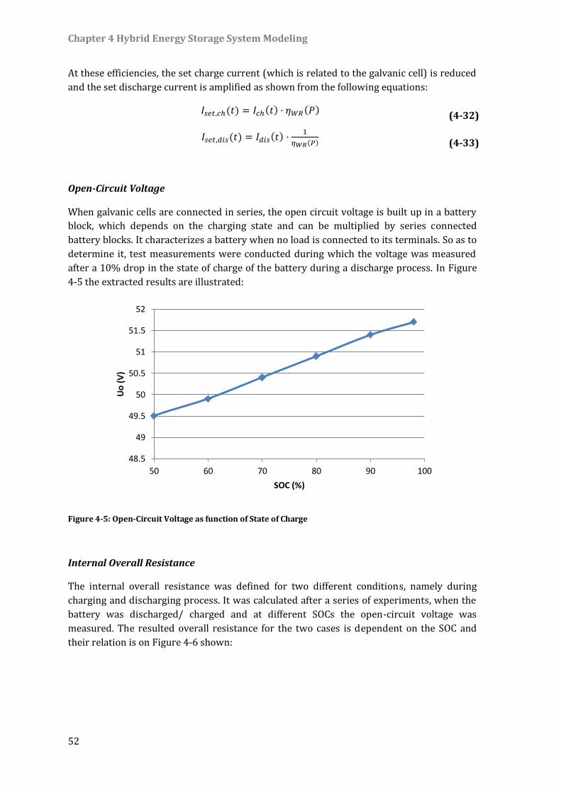
Chapter 4 Hybrid Energy Storage System Modeling
52
At these efficiencies, the set charge current (which is related to the galvanic cell) is reduced
and the set discharge current is amplified as shown from the following equations:
𝐼𝑠𝑒𝑡,𝑐ℎ(𝑡) = 𝐼𝑐ℎ(𝑡) · 𝜂𝑊𝑅(𝑃) (4-32)
𝐼𝑠𝑒𝑡,𝑑𝑖𝑠(𝑡) = 𝐼𝑑𝑖𝑠(𝑡) ·1
𝜂𝑊𝑅(𝑃)
(4-33)
Open-Circuit Voltage
When galvanic cells are connected in series, the open circuit voltage is built up in a battery
block, which depends on the charging state and can be multiplied by series connected
battery blocks. It characterizes a battery when no load is connected to its terminals. So as to
determine it, test measurements were conducted during which the voltage was measured
after a 10% drop in the state of charge of the battery during a discharge process. In Figure
4-5 the extracted results are illustrated:
Figure 4-5: Open-Circuit Voltage as function of State of Charge
Internal Overall Resistance
The internal overall resistance was defined for two different conditions, namely during
charging and discharging process. It was calculated after a series of experiments, when the
battery was discharged/ charged and at different SOCs the open-circuit voltage was
measured. The resulted overall resistance for the two cases is dependent on the SOC and
their relation is on Figure 4-6 shown:
48.5
49
49.5
50
50.5
51
51.5
52
50 60 70 80 90 100
Uo
(V
)
SOC (%)
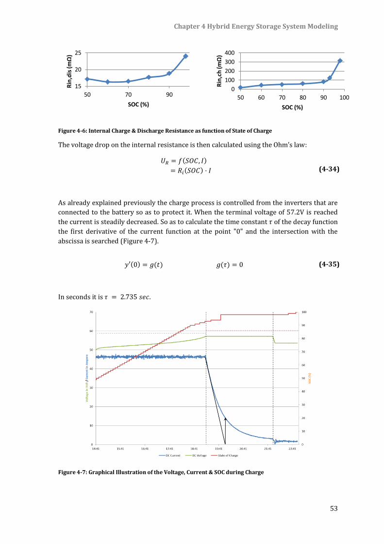
Chapter 4 Hybrid Energy Storage System Modeling
53
Figure 4-6: Internal Charge & Discharge Resistance as function of State of Charge
The voltage drop on the internal resistance is then calculated using the Ohm’s law:
𝑈𝑅 = 𝑓(𝑆𝑂𝐶, 𝐼)
= 𝑅𝑖(𝑆𝑂𝐶) · 𝐼 (4-34)
As already explained previously the charge process is controlled from the inverters that are
connected to the battery so as to protect it. When the terminal voltage of 57.2V is reached
the current is steadily decreased. So as to calculate the time constant 𝜏 of the decay function
the first derivative of the current function at the point "0" and the intersection with the
abscissa is searched (Figure 4-7).
𝑦′(0) = 𝑔(𝑡) 𝑔(𝜏) = 0 (4-35)
In seconds it is 𝜏 = 2.735 𝑠𝑒𝑐.
Figure 4-7: Graphical Illustration of the Voltage, Current & SOC during Charge
15
20
25
50 70 90
Rin
,dis
(mΩ
)
SOC (%)
0
100
200
300
400
50 60 70 80 90 100
Rin
,ch
(mΩ
)
SOC (%)
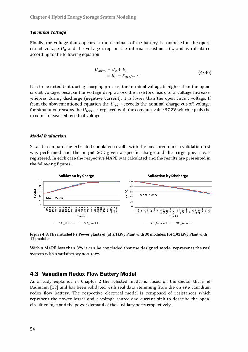
Chapter 4 Hybrid Energy Storage System Modeling
54
Terminal Voltage
Finally, the voltage that appears at the terminals of the battery is composed of the open-
circuit voltage 𝑈0 and the voltage drop on the internal resistance 𝑈𝑅 and is calculated
according to the following equation:
𝑈𝑡𝑒𝑟𝑚 = 𝑈0 + 𝑈𝑅
= 𝑈0 + 𝑅𝑑𝑖𝑠 𝑐ℎ⁄ · 𝐼 (4-36)
It is to be noted that during charging process, the terminal voltage is higher than the open-
circuit voltage, because the voltage drop across the resistors leads to a voltage increase,
whereas during discharge (negative current), it is lower than the open circuit voltage. If
from the abovementioned equation the 𝑈𝑡𝑒𝑟𝑚 exceeds the nominal charge cut-off voltage,
for simulation reasons the 𝑈𝑡𝑒𝑟𝑚 is replaced with the constant value 57.2V which equals the
maximal measured terminal voltage.
Model Evaluation
So as to compare the extracted simulated results with the measured ones a validation test
was performed and the output SOC given a specific charge and discharge power was
registered. In each case the respective MAPE was calculated and the results are presented in
the following figures:
Figure 4-8: The installed PV Power plants of (a) 5.1kWp Plant with 30 modules; (b) 1.02kWp Plant with 12 modules
With a MAPE less than 3% it can be concluded that the designed model represents the real
system with a satisfactory accuracy.
4.3 Vanadium Redox Flow Battery Model
As already explained in Chapter 2 the selected model is based on the doctor thesis of
Baumann [18] and has been validated with real data stemming from the on-site vanadium
redox flow battery. The respective electrical model is composed of resistances which
represent the power losses and a voltage source and current sink to describe the open-
circuit voltage and the power demand of the auxiliary parts respectively.
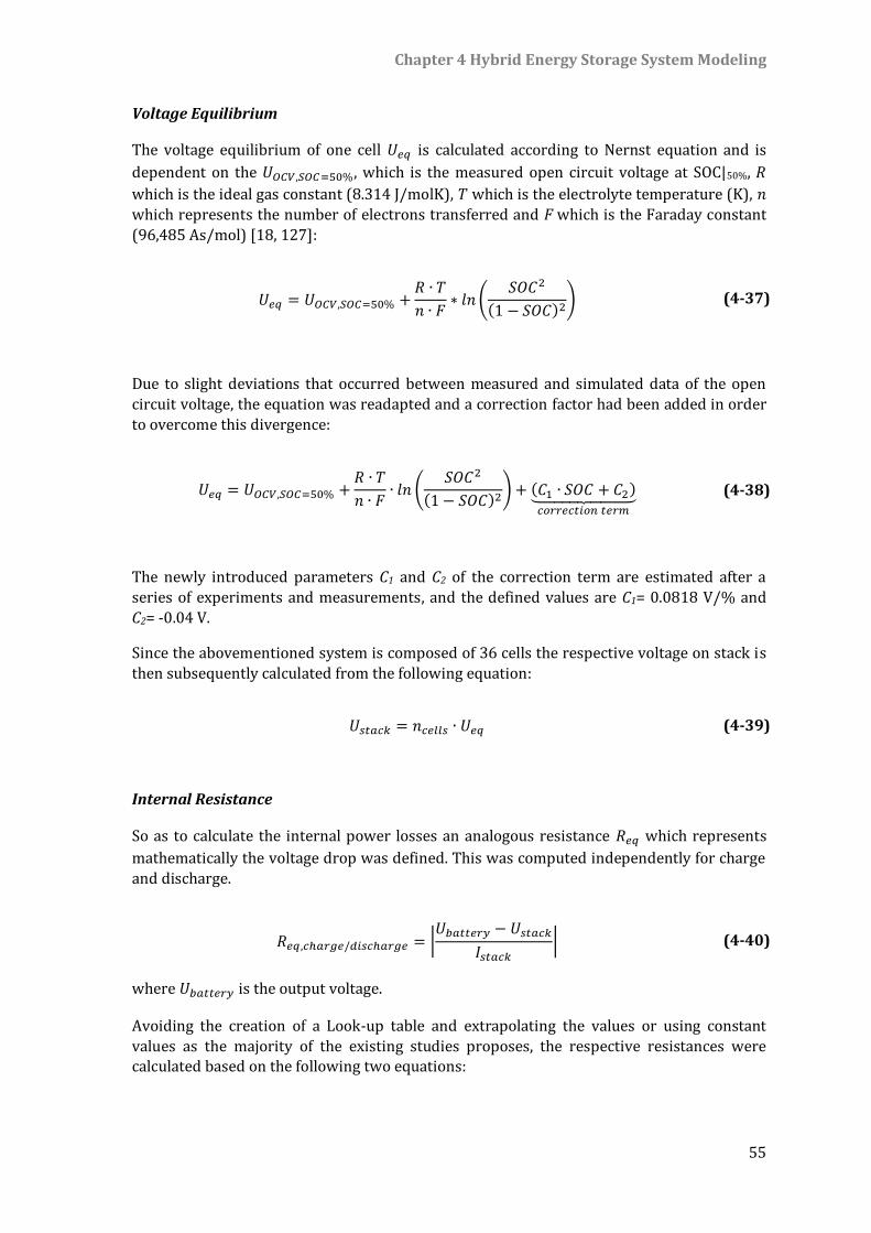
Chapter 4 Hybrid Energy Storage System Modeling
55
Voltage Equilibrium
The voltage equilibrium of one cell 𝑈𝑒𝑞 is calculated according to Nernst equation and is
dependent on the 𝑈𝑂𝐶𝑉,𝑆𝑂𝐶=50%, which is the measured open circuit voltage at SOC|50%, 𝑅
which is the ideal gas constant (8.314 J/molK), 𝑇 which is the electrolyte temperature (K), 𝑛
which represents the number of electrons transferred and F which is the Faraday constant
(96,485 As/mol) [18, 127]:
𝑈𝑒𝑞 = 𝑈𝑂𝐶𝑉,𝑆𝑂𝐶=50% +𝑅 ∙ 𝑇
𝑛 ∙ 𝐹∗ 𝑙𝑛 (
𝑆𝑂𝐶2
(1 − 𝑆𝑂𝐶)2) (4-37)
Due to slight deviations that occurred between measured and simulated data of the open
circuit voltage, the equation was readapted and a correction factor had been added in order
to overcome this divergence:
𝑈𝑒𝑞 = 𝑈𝑂𝐶𝑉,𝑆𝑂𝐶=50% +𝑅 ∙ 𝑇
𝑛 ∙ 𝐹∙ 𝑙𝑛 (
𝑆𝑂𝐶2
(1 − 𝑆𝑂𝐶)2) + (𝐶1 ∙ 𝑆𝑂𝐶 + 𝐶2)⏟
𝑐𝑜𝑟𝑟𝑒𝑐𝑡𝑖𝑜𝑛 𝑡𝑒𝑟𝑚
(4-38)
The newly introduced parameters C1 and C2 of the correction term are estimated after a
series of experiments and measurements, and the defined values are C1= 0.0818 V/% and
C2= -0.04 V.
Since the abovementioned system is composed of 36 cells the respective voltage on stack is
then subsequently calculated from the following equation:
𝑈𝑠𝑡𝑎𝑐𝑘 = 𝑛𝑐𝑒𝑙𝑙𝑠 ∙ 𝑈𝑒𝑞 (4-39)
Internal Resistance
So as to calculate the internal power losses an analogous resistance 𝑅𝑒𝑞 which represents
mathematically the voltage drop was defined. This was computed independently for charge
and discharge.
𝑅𝑒𝑞,𝑐ℎ𝑎𝑟𝑔𝑒/𝑑𝑖𝑠𝑐ℎ𝑎𝑟𝑔𝑒 = |𝑈𝑏𝑎𝑡𝑡𝑒𝑟𝑦 − 𝑈𝑠𝑡𝑎𝑐𝑘
𝐼𝑠𝑡𝑎𝑐𝑘| (4-40)
where 𝑈𝑏𝑎𝑡𝑡𝑒𝑟𝑦 is the output voltage.
Avoiding the creation of a Look-up table and extrapolating the values or using constant
values as the majority of the existing studies proposes, the respective resistances were calculated based on the following two equations:
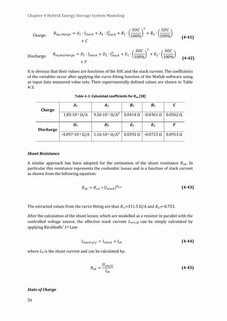
Chapter 4 Hybrid Energy Storage System Modeling
56
Charge: 𝑅𝑒𝑞,𝑐ℎ𝑎𝑟𝑔𝑒 = 𝐴1 ∙ 𝐼𝑠𝑡𝑎𝑐𝑘 + 𝐴2 ∙ 𝐼𝑠𝑡𝑎𝑐𝑘2 + 𝐵1 ∙ (
𝑆𝑂𝐶
100%)2
+ 𝐵2 ∙ (𝑆𝑂𝐶
100%)
+ 𝐶 (4-41)
Discharge: 𝑅𝑒𝑞,𝑑𝑖𝑠𝑐ℎ𝑎𝑟𝑔𝑒 = 𝐷1 ∙ 𝐼𝑠𝑡𝑎𝑐𝑘 + 𝐷2 ∙ 𝐼𝑠𝑡𝑎𝑐𝑘2 + 𝐸1 ∙ (
𝑆𝑂𝐶
100%)2
+ 𝐸2 ∙ (𝑆𝑂𝐶
100%)
+ 𝐹 (4-42)
It is obvious that their values are functions of the SOC and the stack current. The coefficients
of the variables occur after applying the curve fitting function of the Matlab software using
as input data measured value sets. Their experimentally defined values are shown in Table
4-3:
Table 4-3: Calculated coefficients for Req [18]
Charge A1 A2 B1 B2 C
1.85∙10-4 Ω/A 9.36∙10-7 Ω/A² 0.0414 Ω -0.0361 Ω 0.0562 Ω
Discharge D1 D2 E1 E2 F
-4.097∙10-4 Ω/A 1.16∙10-6 Ω/A² 0.0592 Ω -0.0723 Ω 0.0913 Ω
Shunt Resistance
A similar approach has been adopted for the estimation of the shunt resistance 𝑅𝑠ℎ . In
particular this resistance represents the coulombic losses and is a function of stack current
as shown from the following equation:
𝑅𝑠ℎ = 𝑅𝑠,1 ∗ |𝐼𝑠𝑡𝑎𝑐𝑘|𝑅𝑠,2 (4-43)
The extracted values from the curve fitting are thus Rs,1=311.5 Ω/A and Rs,2=-0.753.
After the calculation of the shunt losses, which are modelled as a resistor in parallel with the
controlled voltage source, the effective stack current Istack,eff can be simply calculated by
applying Kirchhoffs’ 1st Law:
𝐼𝑠𝑡𝑎𝑐𝑘,𝑒𝑓𝑓 = 𝐼𝑠𝑡𝑎𝑐𝑘 + 𝐼𝑠ℎ (4-44)
where Ish is the shunt current and can be calculated by:
𝑅𝑠ℎ =𝑈𝑠𝑡𝑎𝑐𝑘𝐼𝑠ℎ
(4-45)
State of Charge
Chapter 4 Hybrid Energy Storage System Modeling
57
The SOC of the system is continuously predicted based on the open circuit voltage of a single
reference cell. It is mathematically extracted from its value on time step 𝑡 − 1 and the
difference occurred in the next time step 𝑡 and is expressed as a fraction of the stored
energy to the maximum energy capacity of the battery:
𝑆𝑂𝐶𝑡=𝑛 = 𝑆𝑂𝐶𝑡=𝑛−1 + ∆𝑆𝑂𝐶 = 𝑆𝑂𝐶𝑡=𝑛−1 +∫𝑛𝑐𝑒𝑙𝑙𝑠 ∙ 𝑈𝑒𝑞 ∙ 𝐼𝑠𝑡𝑎𝑐𝑘,𝑒𝑓𝑓
𝐸𝑐𝑎𝑝𝑎𝑐𝑖𝑡𝑦
𝑛
𝑡=𝑛−1
𝑑𝑡 (4-46)
At this point it should be noted that between the calculation from the controller of the SOC
and the mixing of the electrolyte in the tanks a time delay is noticed which is approximately
six minutes according to measurements and is in the model integrated through the
abovementioned equation.
Approximation of power consumption of the auxiliary devices
The last step to be taken into account for modelling the vanadium redox flow battery is the
estimation of the power needed to supply the BOP system which actually supplies the
actuators, the pumps and the sensors with the required energy.
Due to the fact that the electrolyte pumps are consuming a substantial amount of power but
no hydraulic model has been developed or integrated to the current model because a more
electrical approach was chosen, the power demand was defined based on the different
states of charge and the respective stack current. In each case and after a series of
experiments a power demand estimation was defined as shown in Table 4-4:
Table 4-4: Estimated Power Consumption of the Auxiliary Systems [18]
𝑰𝒔𝒕𝒂𝒄𝒌 𝑺𝑶𝑪 < 𝟑𝟔% 𝟑𝟔% < 𝑺𝑶𝑪 ≤ 𝟔𝟔.𝟐% 𝑺𝑶𝑪 > 𝟔𝟔.𝟐%
𝟎 > 𝑰𝒔𝒕𝒂𝒄𝒌 > −𝟓𝟎𝑨 500 W
𝑰𝒔𝒕𝒂𝒄𝒌 ≤ −𝟓𝟎𝑨 520 W
𝟎 < 𝑰𝒔𝒕𝒂𝒄𝒌 ≤ 𝟑𝟓𝑨 225 W 177 W 228 W
𝟑𝟓𝑨 < 𝑰𝒔𝒕𝒂𝒄𝒌 ≤ 𝟖𝟎𝑨 360 W 260 W 365 W
𝑰𝒔𝒕𝒂𝒄𝒌 > 𝟖𝟎𝑨 508 W 365 W 518 W
Finally the output system power is given from the following equation:
𝑃𝑠𝑦𝑠𝑡𝑒𝑚 = 𝑃𝑠𝑡𝑎𝑐𝑘 − 𝑃𝑎𝑢𝑥 (4-47)
Model Evaluation
All these individual modelling parts were integrated into one single model in Matlab/
Simulink environment and finally a validation test was conducted to prove the accordance
of the simulated with the measured data during charge and discharge process. With a MAPE
of 0.5% it can be concluded that the simulated model represents sufficiently the
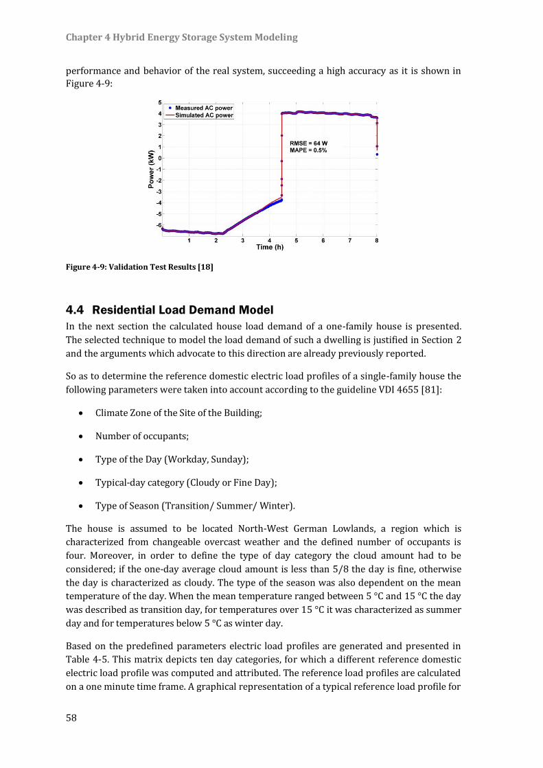
Chapter 4 Hybrid Energy Storage System Modeling
58
performance and behavior of the real system, succeeding a high accuracy as it is shown in
Figure 4-9:
Figure 4-9: Validation Test Results [18]
4.4 Residential Load Demand Model
In the next section the calculated house load demand of a one-family house is presented.
The selected technique to model the load demand of such a dwelling is justified in Section 2
and the arguments which advocate to this direction are already previously reported.
So as to determine the reference domestic electric load profiles of a single-family house the
following parameters were taken into account according to the guideline VDI 4655 [81]:
Climate Zone of the Site of the Building;
Number of occupants;
Type of the Day (Workday, Sunday);
Typical-day category (Cloudy or Fine Day);
Type of Season (Transition/ Summer/ Winter).
The house is assumed to be located North-West German Lowlands, a region which is
characterized from changeable overcast weather and the defined number of occupants is
four. Moreover, in order to define the type of day category the cloud amount had to be
considered; if the one-day average cloud amount is less than 5/8 the day is fine, otherwise
the day is characterized as cloudy. The type of the season was also dependent on the mean
temperature of the day. When the mean temperature ranged between 5 °C and 15 °C the day
was described as transition day, for temperatures over 15 °C it was characterized as summer
day and for temperatures below 5 °C as winter day.
Based on the predefined parameters electric load profiles are generated and presented in
Table 4-5. This matrix depicts ten day categories, for which a different reference domestic
electric load profile was computed and attributed. The reference load profiles are calculated
on a one minute time frame. A graphical representation of a typical reference load profile for
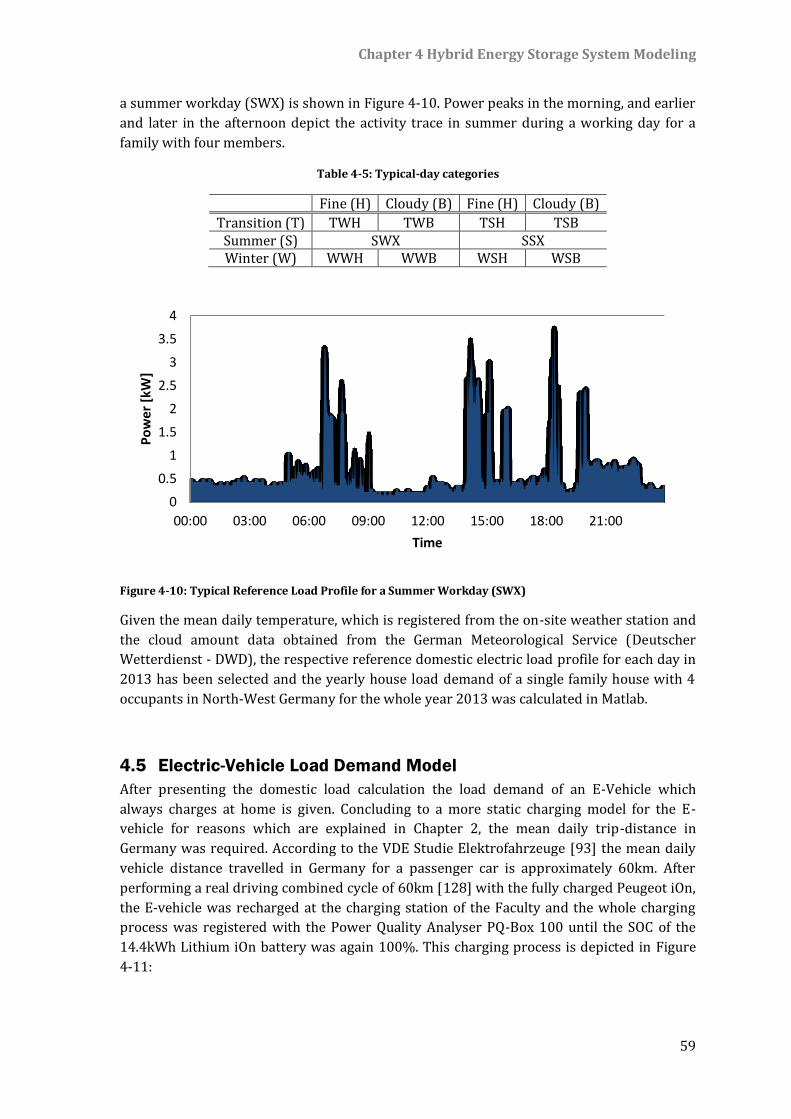
Chapter 4 Hybrid Energy Storage System Modeling
59
a summer workday (SWX) is shown in Figure 4-10. Power peaks in the morning, and earlier
and later in the afternoon depict the activity trace in summer during a working day for a
family with four members.
Table 4-5: Typical-day categories
Fine (H) Cloudy (B) Fine (H) Cloudy (B)
Transition (T) TWH TWB TSH TSB Summer (S) SWX SSX Winter (W) WWH WWB WSH WSB
Figure 4-10: Typical Reference Load Profile for a Summer Workday (SWX)
Given the mean daily temperature, which is registered from the on-site weather station and
the cloud amount data obtained from the German Meteorological Service (Deutscher
Wetterdienst - DWD), the respective reference domestic electric load profile for each day in
2013 has been selected and the yearly house load demand of a single family house with 4
occupants in North-West Germany for the whole year 2013 was calculated in Matlab.
4.5 Electric-Vehicle Load Demand Model
After presenting the domestic load calculation the load demand of an E-Vehicle which
always charges at home is given. Concluding to a more static charging model for the E-
vehicle for reasons which are explained in Chapter 2, the mean daily trip-distance in
Germany was required. According to the VDE Studie Elektrofahrzeuge [93] the mean daily
vehicle distance travelled in Germany for a passenger car is approximately 60km. After
performing a real driving combined cycle of 60km [128] with the fully charged Peugeot iOn,
the E-vehicle was recharged at the charging station of the Faculty and the whole charging
process was registered with the Power Quality Analyser PQ-Box 100 until the SOC of the
14.4kWh Lithium iOn battery was again 100%. This charging process is depicted in Figure
4-11:
0
0.5
1
1.5
2
2.5
3
3.5
4
00:00 03:00 06:00 09:00 12:00 15:00 18:00 21:00
Po
wer
[kW
]
Time
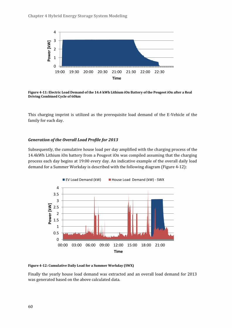
Chapter 4 Hybrid Energy Storage System Modeling
60
Figure 4-11: Electric Load Demand of the 14.4 kWh Lithium iOn Battery of the Peugeot iOn after a Real Driving Combined Cycle of 60km
This charging imprint is utilized as the prerequisite load demand of the E-Vehicle of the
family for each day.
Generation of the Overall Load Profile for 2013
Subsequently, the cumulative house load per day amplified with the charging process of the
14.4kWh Lithium iOn battery from a Peugeot iOn was compiled assuming that the charging
process each day begins at 19:00 every day. An indicative example of the overall daily load
demand for a Summer Workday is described with the following diagram (Figure 4-12):
Figure 4-12: Cumulative Daily Load for a Summer Workday (SWX)
Finally the yearly house load demand was extracted and an overall load demand for 2013
was generated based on the above calculated data.
0
1
2
3
4
19:00 19:30 20:00 20:30 21:00 21:30 22:00 22:30
Po
wer
[kW
]
Time
0
0.5
1
1.5
2
2.5
3
3.5
4
00:00 03:00 06:00 09:00 12:00 15:00 18:00 21:00
Po
wer
[kW
]
Time
EV Load Demand (kW) House Load Demand (kW) - SWX
Chapter 4 Hybrid Energy Storage System Modeling
61
4.6 Grid Model
After covering the individual models that represent an existing physical key element of the
conceptualized system in the previous sections, another block is introduced so as to depict
the occurred power exchange between the building and the grid. In particular, an additional
block is added to the system representation in Matlab/ Simulink which encapsulates and
extracts the 𝑃𝑔𝑟𝑖𝑑(𝑡). This variable is calculated after the energy management system (which
will be presented in detail in Section 5) allocates the arisen power difference (i.e. the
instantaneous local load demand deduced from the respective energy produced from the PV
panels at the same time logging) to the available storage systems. Then another power
balance computation is executed, estimating the residual power that is missing (in case the
local demand is not yet fully covered) or is redundant and must be fed to the public grid and
is described mathematically from the following equations:
𝑃𝑔𝑟𝑖𝑑(𝑡) = 𝑃𝑑𝑖𝑓𝑓(𝑡) − 𝑃𝑏𝑎𝑡𝑡𝑒𝑟𝑦(𝑡) (4-48)
𝑃𝑔𝑟𝑖𝑑(𝑡) = {𝑃𝑔𝑟𝑖𝑑𝑑𝑟𝑎𝑤(𝑡), 𝑖𝑓𝑃𝑔𝑟𝑖𝑑(𝑡) > 0
𝑃𝑔𝑟𝑖𝑑𝑓𝑒𝑒𝑑(𝑡), 𝑖𝑓 𝑃𝑔𝑟𝑖𝑑(𝑡) < 0 (4-49)
Finally, it should be noted that the charging of the batteries from the public grid is
prohibited in this configuration in order to minimize the system losses.

Chapter 4 Hybrid Energy Storage System Modeling
62
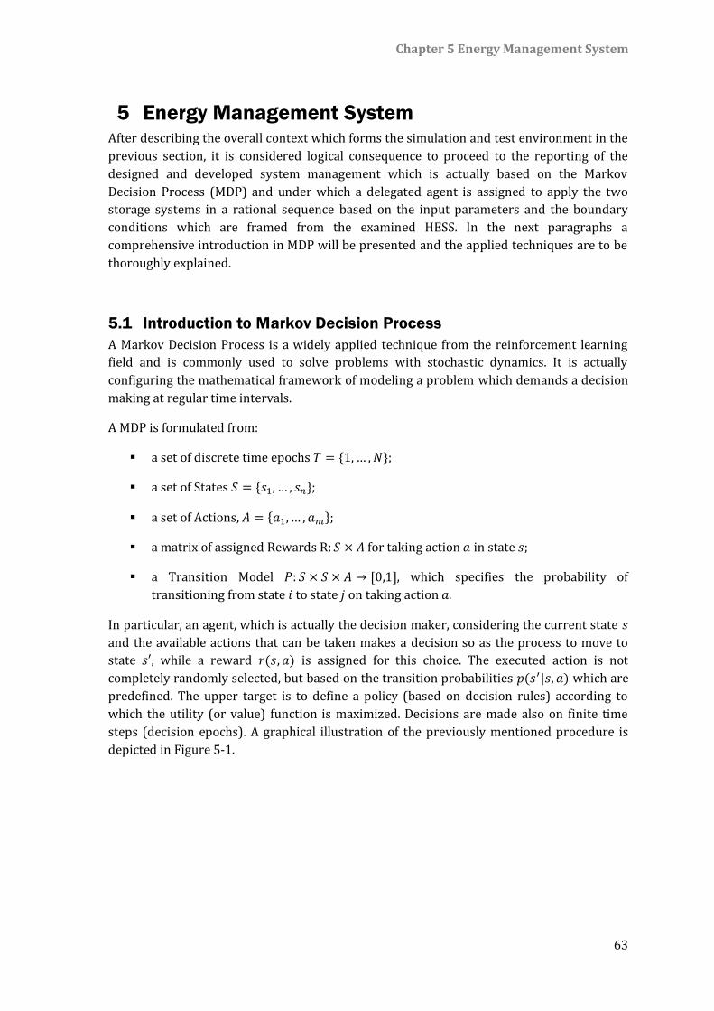
Chapter 5 Energy Management System
63
5 Energy Management System After describing the overall context which forms the simulation and test environment in the
previous section, it is considered logical consequence to proceed to the reporting of the
designed and developed system management which is actually based on the Markov
Decision Process (MDP) and under which a delegated agent is assigned to apply the two
storage systems in a rational sequence based on the input parameters and the boundary
conditions which are framed from the examined HESS. In the next paragraphs a
comprehensive introduction in MDP will be presented and the applied techniques are to be
thoroughly explained.
5.1 Introduction to Markov Decision Process
A Markov Decision Process is a widely applied technique from the reinforcement learning
field and is commonly used to solve problems with stochastic dynamics. It is actually
configuring the mathematical framework of modeling a problem which demands a decision
making at regular time intervals.
A MDP is formulated from:
a set of discrete time epochs 𝑇 = {1,… ,𝑁};
a set of States 𝑆 = {𝑠1, … , 𝑠𝑛};
a set of Actions, 𝐴 = {𝑎1,… , 𝑎𝑚};
a matrix of assigned Rewards R: 𝑆 × 𝐴 for taking action 𝑎 in state 𝑠;
a Transition Model 𝑃: 𝑆 × 𝑆 × 𝐴 → [0,1], which specifies the probability of
transitioning from state 𝑖 to state 𝑗 on taking action 𝑎.
In particular, an agent, which is actually the decision maker, considering the current state 𝑠
and the available actions that can be taken makes a decision so as the process to move to
state 𝑠′, while a reward 𝑟(𝑠, 𝑎) is assigned for this choice. The executed action is not
completely randomly selected, but based on the transition probabilities 𝑝(𝑠′|𝑠, 𝑎) which are
predefined. The upper target is to define a policy (based on decision rules) according to
which the utility (or value) function is maximized. Decisions are made also on finite time
steps (decision epochs). A graphical illustration of the previously mentioned procedure is
depicted in Figure 5-1.
Chapter 5 Energy Management System
64
Figure 5-1: A graphical illustration of a MDP model
Therefore a selection of objects with the structure:
{𝑇, 𝑆, 𝐴𝑠 , 𝑟 (𝑠, 𝑎), 𝑝 }
is formulating a Markov Decision Process.
It is should be noted that according to [129] the reward could be:
a lump sum which is calculated prior to the next discrete time epoch;
computed constantly during the present time epoch;
an ambiguous value which occurs from the system state in the next time epoch;
a blend of the abovementioned cases.
When referring to the type of decision rules that shall be applied different clusters are
identified. We classify the existing decision rules as Markovian or history dependent if the
decision made depends on the previous states only through the current state and or if it is
linked to the history through the whole sequence of applied actions and states respectively.
Moreover the differentiation between randomized and deterministic emerges from the
grade of certainty that characterizes the chosen action.
In a finite horizon problem the Utility function for discounted Markov Decision Problems is
defined as follows:
𝑈(𝑠0 , … . ) = 𝑅(𝑠0) + 𝑅(𝑠1)+. . +𝑅(𝑠𝑁) (5-1)
In the above function the result may be arbitrarily large and the amount of time epochs
must be known in advance. On the other hand, in an infinite horizon problem the Utility
function for discounted Markov Decision Problems is defined as follows:
𝑈(𝑠0, … . ) = 𝑅(𝑠0) + 𝛾𝑅(𝑠1)+. . +𝛾𝑁𝑅(𝑠𝑁)+. . (5-2)
Chapter 5 Energy Management System
65
The parameter 𝛾 is the discount factor and conduces to the convergence of the function. If γ
is close to 0 then more attention is paid on instant gratification and the faster the
convergence is, otherwise (γ close to 1) future rewards are considered more important.
The agent is obliged to find an optimal policy π, which is a sequence of actions, that
maximizes the abovementioned utility function which can be rewritten in a more
generalized form as follows:
𝑈𝜋(𝑠) = 𝑅(𝑠) + 𝛾∑ 𝑇(𝑠, 𝜋(𝑠), 𝑠’) 𝑈𝜋(𝑠’)𝑠’
(5-3)
In general, we need |S|2x|A| numbers to store all the transitions probabilities.
Markov Decision Problems with infinite horizon can be solved based on two different
techniques:
- value iteration;
- policy iteration.
Value iteration is the most widely used tactic to solve indefinite horizon problems. Given the
fact that all the parameters are already known the optimal policy is to be found by solving
the Bellman’s equation:
𝑈𝜋∗(𝑠) = 𝑚𝑎𝑥 [𝑅(𝑠, 𝑎) + 𝛾∑𝑃𝑠𝑠’𝑎
𝑖
𝑈𝜋∗(𝑠’)] (5-4)
where 𝜋∗ is the optimal policy for state 𝑠 and 𝑈𝜋∗ the value of the respective state when the
policy 𝜋∗ is applied.
The abovementioned equation converges and is proved to have a unique solution which is
extracted after multiple iterations of the function. In this case we begin with the
initialization of the value function so as to have a comparison metric for computing the
convergence.
When policy iteration is chosen the agent makes a decision by starting with an arbitrary
policy 𝜋0 and proceeds with the estimation of the utility function. If the convergence
between two consecutive policies is satisfactory then the iteration stops. Otherwise another
policy is selected and the process is repeated. The evaluation criterion remains the
maximization of the following component of the utility function and so is the policy in the
next time step selected. Target is to create a sequence of decision rules and actions where
the respective rewards are monotonically increasing.
𝜋𝑘+1(𝑠) = 𝑎𝑟𝑔𝑚𝑎𝑥(∑𝑃𝑠𝑠’𝑎
𝑖
𝑈𝜋𝑘(𝑠’)) (5-5)
During value iteration the optimal value function is computed and then the policy is
concretized. The optimal value function is attained with convergence after an iterative
approximation. During policy iteration, policy is primarily defined and then the value of the
function is calculated. The method is iteratively transformed till it cannot be further
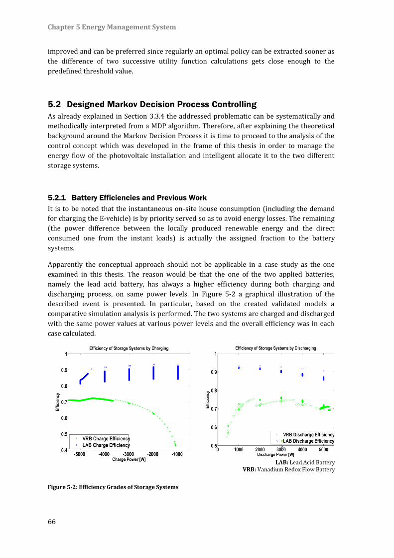
Chapter 5 Energy Management System
66
improved and can be preferred since regularly an optimal policy can be extracted sooner as
the difference of two successive utility function calculations gets close enough to the
predefined threshold value.
5.2 Designed Markov Decision Process Controlling
As already explained in Section 3.3.4 the addressed problematic can be systematically and
methodically interpreted from a MDP algorithm. Therefore, after explaining the theoretical
background around the Markov Decision Process it is time to proceed to the analysis of the
control concept which was developed in the frame of this thesis in order to manage the
energy flow of the photovoltaic installation and intelligent allocate it to the two different
storage systems.
5.2.1 Battery Efficiencies and Previous Work
It is to be noted that the instantaneous on-site house consumption (including the demand
for charging the E-vehicle) is by priority served so as to avoid energy losses. The remaining
(the power difference between the locally produced renewable energy and the direct
consumed one from the instant loads) is actually the assigned fraction to the battery
systems.
Apparently the conceptual approach should not be applicable in a case study as the one
examined in this thesis. The reason would be that the one of the two applied batteries,
namely the lead acid battery, has always a higher efficiency during both charging and
discharging process, on same power levels. In Figure 5-2 a graphical illustration of the
described event is presented. In particular, based on the created validated models a
comparative simulation analysis is performed. The two systems are charged and discharged
with the same power values at various power levels and the overall efficiency was in each
case calculated.
LAB: Lead Acid Battery
VRB: Vanadium Redox Flow Battery
Figure 5-2: Efficiency Grades of Storage Systems
Chapter 5 Energy Management System
67
It is obvious that at first glance there is no need for an energy management system since the
vanadium redox flow battery performs always worse as the lead acid battery. Several
reasons could explain this phenomenon. First, VRBs are still a commercially immature
technology, meaning that there is still a lot to be accomplished so as this battery type to
reach efficiency levels of technologies which are in market for years. In addition, although it
is in literature otherwise argued, the examined system (which is commercially available and
not only a test unit for demos and experiments) is characterized by higher losses as
theoretically claimed if all coulombic and peripheral losses are taken into account.
Nevertheless, it is identified that there are power regions where the VRB has improved
performance records, favoring its function between these areas. The energy management
system is therefore so designed to detect these power ranges and try to operate the VRB at
an overall higher efficiency. This is succeeded through a reward/ penalty policy which is by
default integrated into the MDP and was respectively adapted.
A similar approach is also adopted in the study of Qiu [17]. A thorough description of this
case is presented in Section 3.3.4 though it should be stressed out here that although the
examined systems appear ostensibly to have a similar structure the internal characteristics
of the storage systems have in Qiu’s study dictated a different handling method in designing
the respective control unit. In particular, the efficiency grades of the selected storage
systems in that case intersect at a power level, setting the implementation of a MDP as more
trivial as in any other case. To this respect the applied method cannot be generalized in
cases when the adopted systems efficiency curves do not have an intersection point, as it is
in this case study. Therefore it was decided it was acute to develop a new MDP algorithm
which would also incorporate more system configurations.
5.2.2 Markov Process of the Examined System
The designed discrete MDP includes the definition of the various states, actions, rewards
and transition probabilities and are in detail analyzed in the following section. A design
approach with a continuous state MDP is not attempted in the frame of this thesis since
according to literature continuous MDP problems are mainly solved through discretization
of the states, leading thus to an exponential increase of the number of states [130]. In
addition, as it subsequently described the state space is already sufficiently fragmented
representing a considerable amount of states.
It should be also stated that target of this study is not to recognize the optimal storage
capacities’ combination that can be coupled with the given size of the PV installation and the
type of domestic load demand, which is extracted as it is described in Sections 4.4 and 4.5,
rather it was attempted to identify a method that can optimally allocate/ serve the available
power excess or occurring power demand in an experimental space with predefined storage
types and sizes, which though remain in a scale that matches the needs of a dwelling with
such a load time series and an on-site PV power generation, in order to succeed grid
stability.
Chapter 5 Energy Management System
68
States’ Definition
The decision of the states’ choice is key constituent for the overall process and before
proceeding to its definition it is considered wise to assess what a meaningful state space
stands for. The determination of the variables that should be integrated in the state matrix
must be carefully selected so as to attribute the model needs and the environment
characteristics to the control management unit, without exaggerating in the contained
information and by keeping the content fully observable. The energy management unit
should allocate the arising power difference after consideration of the SOC of the respective
storage system. The physical characteristics of the batteries, such as the internal resistances
or the maximum current are not considered here, since they are in modelling part
integrated. On the other hand, the capacity of the systems, which is obliquely related to the
SOC, as well as the value of the arising power difference are affecting the design part. In the
examined case the selected states were defined from the state of charge of the two storage
systems and the power difference which constitutes the demand or the surplus of energy
which arises after subtracting the instant power demand from the on-site renewable energy
generation.
It should be noted that the applied technique as concept is identical during charge and
discharge phases and differentiates only numerically by the different efficiencies of the
storage systems which are given as input to the MDP algorithm.
In particular, the range of the arising power difference was divided in six discrete intervals
from [0… 6𝑘𝑊] (the occurring 𝑃𝑑𝑖𝑓𝑓 was extended in this range; in any other case the limits
can be accordingly scaled). The designed algorithm observes the sign of the parameter
(negative 𝑃𝑑𝑖𝑓𝑓 corresponds to power excess and positive value to power deficit) and
applies respectively the matching method. The SOC ranges were respectively defined by
creating SOC level partitions, one for each system. The lead acid battery, whose minimal SOC
is limited to 50% of the installed capacity, has a SOC range from [0…10] in the designed
MDP, and the SOC of the vanadium redox flow battery is described from a range of states in
the scale from [0…20]. These SOC ranges were selected based on the capacities of the
storage systems. In particular, the useable SOC range of the VRB (33% till 74%) corresponds
to a stored energy of almost 20 kWh, while the lead acid battery, with an exploitable SOC
above 50% for safety reasons is with only 10 kWh full. The numerical interpretation of these
discretized states is experimentally investigated and a trial-and-error process advocated for
the empirical distributions:
𝑆𝑂𝐶𝐿𝐴𝐵 = {[0 0.5) , [0.5 0.545), [0.545 0.59)⋯ [0.905 1] } (5-6)
𝑆𝑂𝐶𝑉𝑅𝐹𝐵 = {[0 0.33) , [0.33 0.3505)⋯ [0.699 0.7195 ), [0.7195 0.74] } (5-7)
𝑃𝑑𝑖𝑓𝑓 (𝑊) = {[0 1000) , [1000 2000)⋯ [4000 5000), [5000 6000] } (5-8)
So each defined state is represented in the model as follows:
Chapter 5 Energy Management System
69
𝑆𝑛𝑖,𝑗,𝑘 = {𝑆𝑂𝐶𝐿𝐴𝐵𝑖 , 𝑆𝑂𝐶𝑉𝑅𝐹𝐵𝑗 , 𝑃𝑑𝑖𝑓𝑓𝑘} , 𝑖 = 1⋯11, 𝑗 = 1⋯21, 𝑘 = 1⋯6, 𝑛 = 1⋯𝑁,
𝑁 = 𝑖 ∙ 𝑗 ∙ 𝑘 (5-9) 0
Actions’ Definition
After specifying the selected states and composing the state space the actions that can be
taken are defined. These are namely the command to charge/discharge the lead acid battery
system (𝐴𝐿𝐴𝐵) or the vanadium redox flow battery (𝐴𝑉𝐹𝑅𝐵) or to perform no action (𝐴𝑛𝑜𝑛𝑒).
At this point it should be stressed out that for each time interval only one battery may
operate and the occurred power difference is not divided in arbitrary or analogous to the
each system characteristics partitions. The actions’ set 𝛢 contains the three distinct actions :
𝛢 = {𝐴𝐿𝐴𝐵 , 𝐴𝑉𝐹𝑅𝐵, 𝐴𝑛𝑜𝑛𝑒} (5-10)
Rewards’ Definition
The instant reward is respectively formulated based on the efficiency of the two storage
systems at each charge/ discharge level. This was calculated by estimating the instant
power losses according to the efficiency grade that each system is attributed with at the
respective power level (see Figure 5-2). In addition reward takes into account special cases
like avoiding charging a fully charged battery and preventing charging none of the batteries
when both batteries are not fully charged.
In general, except for the special cases mentioned above, the instant reward 𝑅 is defined as
follows:
𝑅 = −|𝑃𝑙𝑜𝑠𝑠| (5-11)
Since the charge power states 𝑃𝑑𝑖𝑓𝑓 include a range of values and due to the non-linearity of
the efficiency curves, due to the fact that the efficiency is dependent not only to the power
value but also to the current SOC as illustrated in Figure 5-2, we have to assume that for
each 𝑃𝑑𝑖𝑓𝑓𝑘, the batteries have a constant 𝐸𝑓𝑓𝐿𝐴𝐵𝑘 and 𝐸𝑓𝑓𝑉𝐹𝑅𝐵𝑘 correspondingly. This
assumption applies only for the calculation of the rewards and not when modeling the
battery performance later. By definition the useable amount of power is the product of the
power difference to the respective facility efficiency (𝑃𝑢𝑠𝑒𝑎𝑏𝑙𝑒 = 𝐸𝑓𝑓 ∗ 𝑃𝑑𝑖𝑓𝑓). So the losses
which are in the designed algorithm the opposite of the reward function, occur from the
complement of the useable power (𝑃𝑙𝑜𝑠𝑠= ( 1 − 𝐸𝑓𝑓) ∗ 𝑃𝑑𝑖𝑓𝑓). The reward is calculated as
following:
Chapter 5 Energy Management System
70
𝑅(𝑠, 𝑎)|𝑠∈𝑆,𝑎𝜖𝐴 =
{
(𝐸𝑓𝑓𝐿𝐴𝐵𝑘 − 1) ∙ 𝑃𝑑𝑖𝑓𝑓𝑘∶ 𝑎 = 𝐴𝐿𝐴𝐵
(𝐸𝑓𝑓𝑉𝐹𝑅𝐵𝑘 − 1) ∙ 𝑃𝑑𝑖𝑓𝑓𝑘: , 𝑎 = 𝐴𝑉𝐹𝑅𝐵
−𝑐1 ∶ 𝑎 = 𝐴𝑛𝑜𝑛𝑒 , 𝑆𝑂𝐶𝐿𝐴𝐵𝑖|𝑖≠11 , 𝑆𝑂𝐶𝑉𝐹𝑅𝐵𝑗|𝑗≠21
0 ∶ 𝑎 = 𝐴𝑛𝑜𝑛𝑒 , 𝑆𝑂𝐶𝐿𝐴𝐵𝑖|𝑖=11, 𝑆𝑂𝐶𝑉𝐹𝑅𝐵𝑗|𝑗=21
−𝑐1 ∶ 𝑎 = 𝐴𝐿𝐴𝐵 , 𝑆𝑂𝐶𝐿𝐴𝐵𝑖|𝑖=11−𝑐1 ∶ 𝑎 = 𝐴𝑉𝐹𝑅𝐵, 𝑆𝑂𝐶𝑉𝐹𝑅𝐵𝑗|𝑗=21
(5-12)
In cases when the system decides to take no action, the reward is either an arbitrary large
negative reward " − 𝑐1" (lowest than any other assignable reward) if both batteries are not
fully charged (line 3 in Equation (5-12)) or 0 (the highest assigned reward) if both batteries
are full (line 4 in Equation (5-12)). In cases that the action tries to charge an already fully
charged battery (lines 5 and 6 in Equation (5-12)), the same large negative value is assigned
in order to prevent such actions being preferred.
Transition Probabilities’ Definition
The last step is to calculate the state transition probabilities. As it is in the MDP theory
stated, the new state which is reached after taking an action depends only on the previous
state and the decided action and it is not affected from the previously states [129]. This
involves calculating for a given charge power 𝑃𝑑𝑖𝑓𝑓𝑡 and battery SOC at time step 𝑡 the
transition probability 𝑃𝑠,𝑠′𝑎 when performing action 𝑎:
𝑃𝑠,𝑠′𝑎 = 𝑃(𝑠𝑡+1 = 𝑠
′|𝑠𝑡 = 𝑠, 𝑎 = 𝑎𝑡) (5-13)
In the continuous time space, when the battery has 𝑋𝑡𝑤ℎ Wh stored, after applying a constant
𝑃𝑑𝑖𝑓𝑓 for a given time duration, the energy stored 𝑋𝑡′𝑤ℎ in Wh at time 𝑡′ = 𝑡 + 𝑑𝑡 will be :
𝑋𝑡′𝑤ℎ = 𝑋𝑡
𝑤ℎ + 𝑃𝑑𝑖𝑓𝑓 ∙ Eff ∙ 𝑑𝑡, (5-14)
and by setting 𝑑𝑡 = 1ℎ and 𝐸𝑐ℎ𝑎𝑟𝑔𝑒/𝑑𝑖𝑠𝑐ℎ𝑎𝑟𝑔𝑒 = 𝑃𝑑𝑖𝑓𝑓 ∙ Eff
𝑋𝑡′𝑤ℎ = 𝑋𝑡
𝑤ℎ + 𝐸𝑐ℎ𝑎𝑟𝑔𝑒/𝑑𝑖𝑠𝑐ℎ𝑎𝑟𝑔𝑒 (5-15)
Taking as example the lead acid battery and assuming that the battery state is 𝑆𝑂𝐶𝐿𝐴𝐵𝑖 at
time 𝑡, this means that the actual stored energy 𝑋𝐿𝐴𝐵_𝑡𝑤ℎ is in the range [𝑎𝑖 𝑏𝑖). When
considering the 𝑋𝐿𝐴𝐵_𝑡𝑤ℎ as a uniformly distributed random variable across the boundaries
𝑎𝑖 𝑏𝑖 with probability density function (PDF) 𝑓𝑆(𝑠), and considering also that the 𝐸𝑐ℎ𝑎𝑟𝑔𝑒𝑡 is
also uniformly distributed random variable in the range[𝑎𝑘 𝑏𝑘) with PDF 𝑓𝑃(𝑝), then the
𝑋𝐿𝐴𝐵_𝑡′𝑤ℎ is the convolution of the two distributions [131].
𝑓𝑆′(𝑠′) = ∫ 𝑓𝑆(𝑠)
+∞
−∞
𝑓𝑃(𝑠′ − 𝑠)𝑑𝑠 (5-16)
Now the state transition probabilities can be calculated for each battery (given the state of
the non-charging battery remains the same).
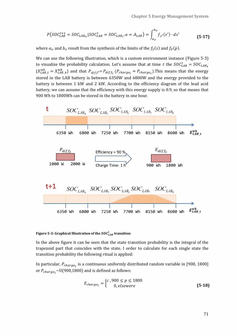
Chapter 5 Energy Management System
71
𝑃(𝑆𝑂𝐶𝐿𝐴𝐵𝑡+1 = 𝑆𝑂𝐶𝐿𝐴𝐵𝑖′ |𝑆𝑂𝐶𝐿𝐴𝐵
𝑡 = 𝑆𝑂𝐶𝐿𝐴𝐵𝑖 , 𝑎 = 𝐴𝐿𝐴𝐵) = ∫ 𝑓𝑠′(𝑠′) ∙
𝑏𝑖′
𝑎𝑖′
𝑑𝑠′ (5-17)
where 𝑎𝑖′ and 𝑏𝑖′ result from the synthesis of the limits of the 𝑓𝑆(𝑠) and 𝑓𝑃(𝑝).
We can use the following illustration, which is a custom environment instance (Figure 5-3)
to visualize the probability calculation. Let’s assume that at time 𝑡 the 𝑆𝑂𝐶𝐿𝐴𝐵𝑡 = 𝑆𝑂𝐶𝐿𝐴𝐵4
(𝑋𝐿𝐴𝐵_𝑡𝑤ℎ = 𝑋𝐿𝐴𝐵_4
𝑤ℎ ) and that 𝑃𝑑𝑖𝑓𝑓𝑡= 𝑃𝑑𝑖𝑓𝑓2 (𝑃𝑐ℎ𝑎𝑟𝑔𝑒𝑡 = 𝑃𝑐ℎ𝑎𝑟𝑔𝑒2).This means that the energy
stored in the LAB battery is between 6350W and 6800W and the energy provided to the
battery is between 1 kW and 2 kW. According to the efficiency diagram of the lead acid
battery, we can assume that the efficiency with this energy supply is 0.9, so that means that
900 Wh to 1800Wh can be stored in the battery in one hour.
Figure 5-3: Graphical Illustration of the 𝑺𝑶𝑪𝑳𝑨𝑩𝒕 transition
In the above figure it can be seen that the state transition probability is the integral of the
trapezoid part that coincides with the state. I order to calculate for each single state the
transition probability the following ritual is applied:
In particular, 𝑃𝑐ℎ𝑎𝑟𝑔𝑒2 is a continuous uniformly distributed random variable in [900, 1800]
or 𝑃𝑐ℎ𝑎𝑟𝑔𝑒2~U(900,1800) and is defined as follows:
𝐸𝑐ℎ𝑎𝑟𝑔𝑒2 = {𝑐 , 900 ≤ 𝑝 ≤ 1800
0, 𝑒𝑙𝑠𝑒𝑤𝑒𝑟𝑒 (5-18)
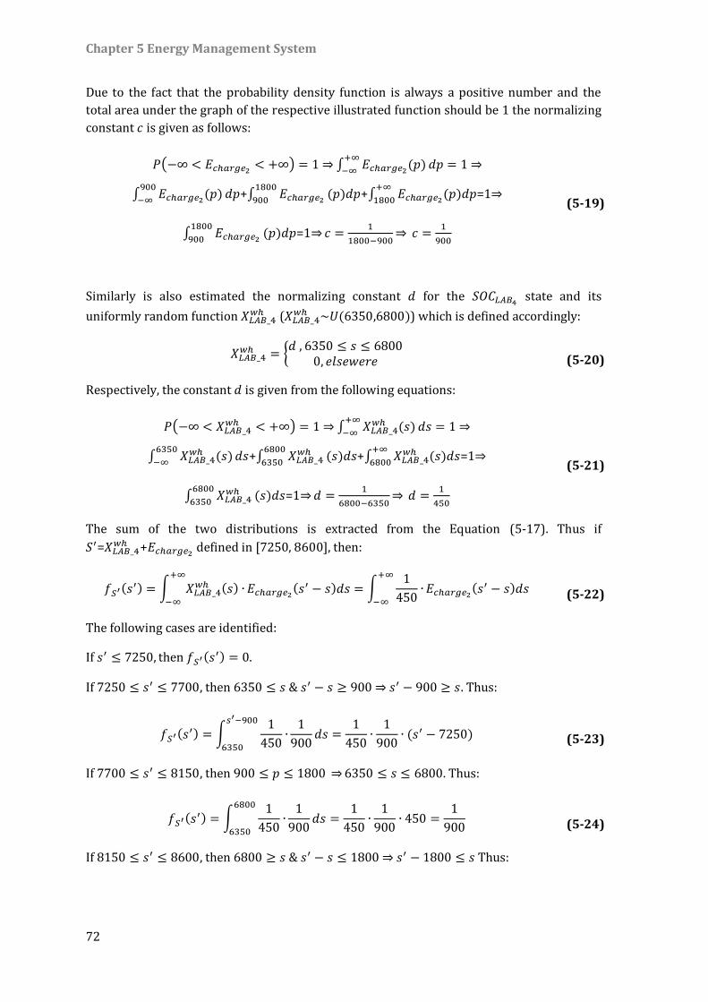
Chapter 5 Energy Management System
72
Due to the fact that the probability density function is always a positive number and the
total area under the graph of the respective illustrated function should be 1 the normalizing
constant 𝑐 is given as follows:
𝑃(−∞ < 𝐸𝑐ℎ𝑎𝑟𝑔𝑒2 < +∞) = 1 ⇒ ∫ 𝐸𝑐ℎ𝑎𝑟𝑔𝑒2(𝑝)+∞
−∞𝑑𝑝 = 1 ⇒
∫ 𝐸𝑐ℎ𝑎𝑟𝑔𝑒2(𝑝)900
−∞𝑑𝑝+∫ 𝐸𝑐ℎ𝑎𝑟𝑔𝑒2
1800
900(𝑝)𝑑𝑝+∫ 𝐸𝑐ℎ𝑎𝑟𝑔𝑒2(𝑝)𝑑𝑝
+∞
1800=1⇒
∫ 𝐸𝑐ℎ𝑎𝑟𝑔𝑒21800
900(𝑝)𝑑𝑝=1⇒𝑐 =
1
1800−900⇒ 𝑐 =
1
900
(5-19)
Similarly is also estimated the normalizing constant 𝑑 for the 𝑆𝑂𝐶𝐿𝐴𝐵4 state and its
uniformly random function 𝑋𝐿𝐴𝐵_4𝑤ℎ (𝑋𝐿𝐴𝐵_4
𝑤ℎ ~𝑈(6350,6800)) which is defined accordingly:
𝑋𝐿𝐴𝐵_4𝑤ℎ = {
𝑑 , 6350 ≤ 𝑠 ≤ 68000, 𝑒𝑙𝑠𝑒𝑤𝑒𝑟𝑒
(5-20)
Respectively, the constant 𝑑 is given from the following equations:
𝑃(−∞ < 𝑋𝐿𝐴𝐵_4𝑤ℎ < +∞) = 1 ⇒ ∫ 𝑋𝐿𝐴𝐵_4
𝑤ℎ (𝑠)+∞
−∞𝑑𝑠 = 1 ⇒
∫ 𝑋𝐿𝐴𝐵_4𝑤ℎ (𝑠)
6350
−∞𝑑𝑠+∫ 𝑋𝐿𝐴𝐵_4
𝑤ℎ6800
6350(𝑠)𝑑𝑠+∫ 𝑋𝐿𝐴𝐵_4
𝑤ℎ (𝑠)𝑑𝑠+∞
6800=1⇒
∫ 𝑋𝐿𝐴𝐵_4𝑤ℎ6800
6350(𝑠)𝑑𝑠=1⇒𝑑 =
1
6800−6350⇒ 𝑑 =
1
450
(5-21)
The sum of the two distributions is extracted from the Equation (5-17). Thus if
𝑆′=𝑋𝐿𝐴𝐵_4𝑤ℎ +𝐸𝑐ℎ𝑎𝑟𝑔𝑒2 defined in [7250, 8600], then:
𝑓𝑆′(𝑠′) = ∫ 𝑋𝐿𝐴𝐵_4
𝑤ℎ (𝑠) ∙+∞
−∞
𝐸𝑐ℎ𝑎𝑟𝑔𝑒2(𝑠′ − 𝑠)𝑑𝑠 = ∫
1
450∙
+∞
−∞
𝐸𝑐ℎ𝑎𝑟𝑔𝑒2(𝑠′ − 𝑠)𝑑𝑠 (5-22)
The following cases are identified:
If 𝑠′ ≤ 7250, then 𝑓𝑆′(𝑠′) = 0.
If 7250 ≤ 𝑠′ ≤ 7700, then 6350 ≤ 𝑠 & 𝑠′ − 𝑠 ≥ 900 ⇒ 𝑠′ − 900 ≥ 𝑠. Thus:
𝑓𝑆′(𝑠′) = ∫
1
450∙
𝑠′−900
6350
1
900𝑑𝑠 =
1
450∙1
900∙ (𝑠′ − 7250) (5-23)
If 7700 ≤ 𝑠′ ≤ 8150, then 900 ≤ 𝑝 ≤ 1800 ⇒6350 ≤ 𝑠 ≤ 6800. Thus:
𝑓𝑆′(𝑠′) = ∫
1
450∙
6800
6350
1
900𝑑𝑠 =
1
450∙1
900∙ 450 =
1
900 (5-24)
If 8150 ≤ 𝑠′ ≤ 8600, then 6800 ≥ 𝑠 & 𝑠′ − 𝑠 ≤ 1800 ⇒ 𝑠′ − 1800 ≤ 𝑠 Thus:
Chapter 5 Energy Management System
73
𝑓𝑆′(𝑠′) = ∫
1
450∙
6800
𝑠′−1800
1
900𝑑𝑠 =
1
450∙1
900∙ (8600 − 𝑠′) (5-25)
If 8600 ≤ 𝑠′, then 𝑓𝑆′(𝑠′) = 0.
Finally, the probability of transition to the new states is the integral of each part of the
newly created piecewise function 𝑓𝑆′(𝑠′) in each respective state space. So:
𝑃(𝑆𝑂𝐶𝐿𝐴𝐵𝑡+1 = 𝑆𝑂𝐶𝐿𝐴𝐵6 |𝑆𝑂𝐶𝐿𝐴𝐵
𝑡 = 𝑆𝑂𝐶𝐿𝐴𝐵4 , 𝑎 = 𝐴𝐿𝐴𝐵) = ∫ 𝑓𝑠′(𝑠′) ∙
7700
7250
𝑑𝑠′
= ∫1
450∙1
900∙ (𝑠′ − 7250)
7700
7250
𝑑𝑠′ = 0.25 (5-26)
𝑃(𝑆𝑂𝐶𝐿𝐴𝐵𝑡+1 = 𝑆𝑂𝐶𝐿𝐴𝐵7 |𝑆𝑂𝐶𝐿𝐴𝐵
𝑡 = 𝑆𝑂𝐶𝐿𝐴𝐵4 , 𝑎 = 𝐴𝐿𝐴𝐵) = ∫ 𝑓𝑠′(𝑠′) ∙
8150
7700
𝑑𝑠′
= ∫1
900
8150
7700
𝑑𝑠′ = 0.5 (5-27)
𝑃(𝑆𝑂𝐶𝐿𝐴𝐵𝑡+1 = 𝑆𝑂𝐶𝐿𝐴𝐵8 |𝑆𝑂𝐶𝐿𝐴𝐵
𝑡 = 𝑆𝑂𝐶𝐿𝐴𝐵4 , 𝑎 = 𝐴𝐿𝐴𝐵) = ∫ 𝑓𝑠′(𝑠′) ∙
8600
8150
𝑑𝑠′
= ∫1
450∙1
900∙ (8600 − 𝑠′)
8600
8150
𝑑𝑠′ = 0.25 (5-28)
This procedure is repeated for every possible SOC of each battery and every possible
provided or requested power difference and in such a way the transition probability matrix
is created and filled with the respectively calculated values. The extracted matrix 𝑁𝑥𝑁𝑥3
combined with the reward vector are the inputs to the Markov model and the optimal policy
is concretized and entered into the Simulink model.
It should be noted that if 𝛢 = {𝐴𝑛𝑜𝑛𝑒} then the 𝑓𝑆′(𝑠′) = 0. Moreover, if the resulting SOC is
beyond the defined ones (the battery cannot accept more energy to be stored), then the
again 𝑓𝑆′(𝑠′) is equal to 0 in that case. In addition an analogous procedure is applied for the
discharge modus. In this case though the trapezoid part has a reverse moving (the stored
energy in the battery is reduced).
Finally, the Utility function integrates the discount factor which is assigned with the value
0.99 for the described method and set to 0.001 if the naive approach is applied.
5.2.3 Implementation
As a basis for the implementation the MDP toolbox [132] was used. MDP toolbox contains
functions related to the resolution of discrete-time Markov Decision Processes and are
Chapter 5 Energy Management System
74
implemented in different programming environments. In this work the Matlab
implementation was used.
In Figure 5-4 the implementation architecture is visualized. Following the logical flow
presented in 5.2.2, in the first step the states and actions are defined. Each state is
represented as a three element vector as described in Equation (5-9):
𝑆(𝑛𝑖,𝑗,𝑘) = [𝑖 𝑗 𝑘], 𝑛 = 1…𝑁 (5-29)
Then by taking in to account the battery efficiencies and Equation (5-17) the state transition
probabilities are calculated as a three dimensional matrix with size 𝑁𝑥𝑁𝑥3. Each element
describes the transition probability between two states with a given action:
𝑃_𝑃𝑟𝑜𝑏(𝑙,𝑚,𝑢) = 𝑃(𝑆𝑙𝑡+1|𝑆𝑚
𝑡 , 𝑎 = 𝐴𝑢)|𝐴𝑢∈𝐴,𝑆𝑙𝑡𝑆𝑚𝑡 ∈𝑆
(5-30)
The last programming step involves the calculation of the rewards, which are also described
in a matrix with size 𝑁𝑥3 and calculated according to Equation (5-12). The reward of an
action 𝑎 = 𝐴𝑢 at state 𝑆𝑛𝑡 is 𝑅(𝑛, 𝑢). The matrixes 𝑃_𝑃𝑟𝑜𝑏 and 𝑅(𝑛, 𝑢) are then given as input
to the MDP Toolbox which performs the Markov optimization process. The result is a vector
with 𝑁 elements containing the optimal policy for each state. This vector is then used by the
Simulink model in the simulation environment. The policy iteration is the applied method
for the resolution of discounted MDP.
In the Simulink model the arising power difference between the load demand and the PV
generation is assigned to the respective 𝑃𝑑𝑖𝑓𝑓𝑡 and the same is repeated for each state of
charge of the two batteries (𝑆𝑂𝐶𝐿𝐴𝐵𝑡 , 𝑆𝑂𝐶𝑉𝑅𝐵
𝑡 ). The sign of the occurred 𝑃𝑑𝑖𝑓𝑓𝑡 activates the
correct algorithm (“-“ stands for excess of energy, thus “Charge modus”, and “+” stands for
demand, thus “Discharge modus” should be triggered). According to these three elements
the optimal action is chosen based on the predefined optimal MDP policy and the
corresponding control command is passed on to the chosen battery.
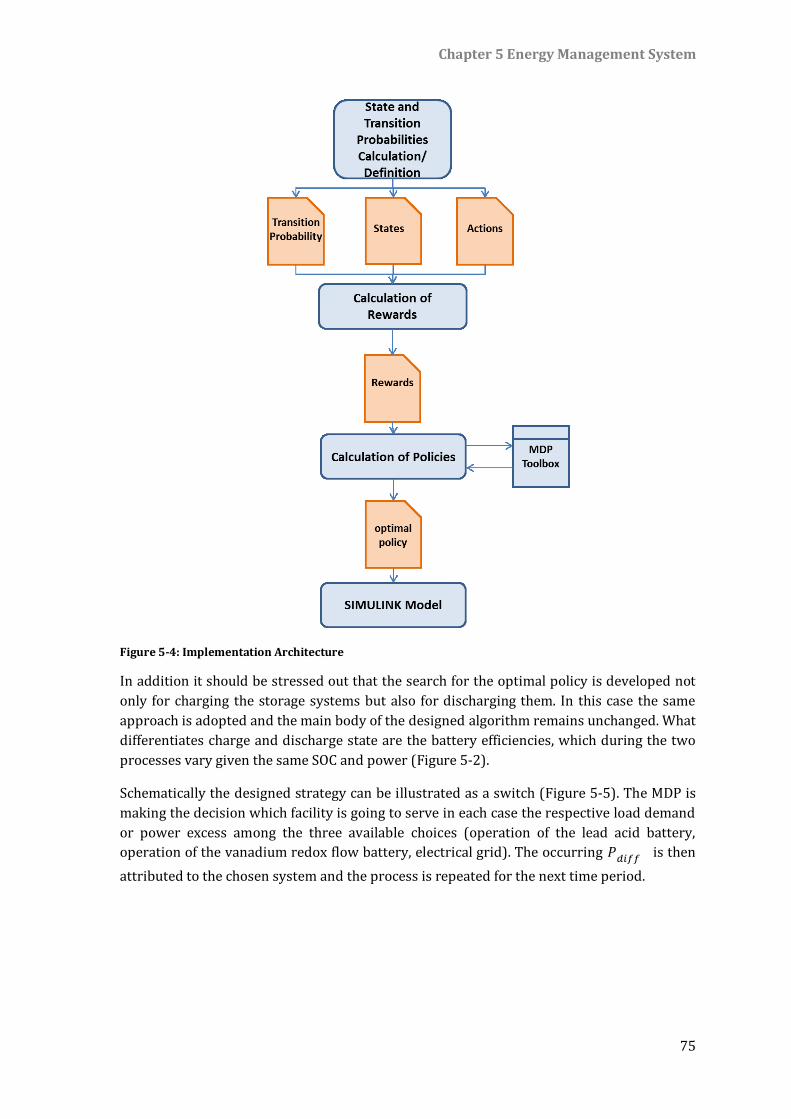
Chapter 5 Energy Management System
75
Figure 5-4: Implementation Architecture
In addition it should be stressed out that the search for the optimal policy is developed not
only for charging the storage systems but also for discharging them. In this case the same
approach is adopted and the main body of the designed algorithm remains unchanged. What
differentiates charge and discharge state are the battery efficiencies, which during the two
processes vary given the same SOC and power (Figure 5-2).
Schematically the designed strategy can be illustrated as a switch (Figure 5-5). The MDP is
making the decision which facility is going to serve in each case the respective load demand
or power excess among the three available choices (operation of the lead acid battery,
operation of the vanadium redox flow battery, electrical grid). The occurring 𝑃𝑑𝑖𝑓𝑓 is then
attributed to the chosen system and the process is repeated for the next time period.
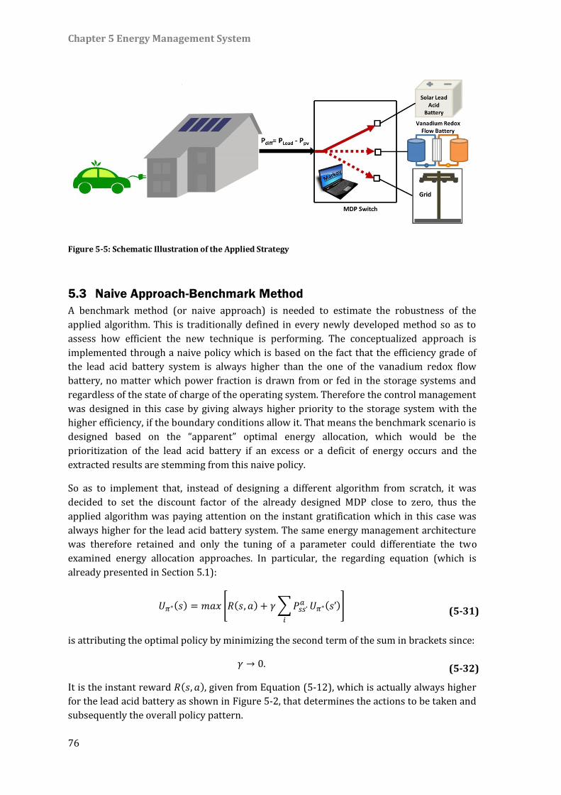
Chapter 5 Energy Management System
76
Figure 5-5: Schematic Illustration of the Applied Strategy
5.3 Naive Approach-Benchmark Method
A benchmark method (or naive approach) is needed to estimate the robustness of the
applied algorithm. This is traditionally defined in every newly developed method so as to
assess how efficient the new technique is performing. The conceptualized approach is
implemented through a naive policy which is based on the fact that the efficiency grade of
the lead acid battery system is always higher than the one of the vanadium redox flow
battery, no matter which power fraction is drawn from or fed in the storage systems and
regardless of the state of charge of the operating system. Therefore the control management
was designed in this case by giving always higher priority to the storage system with the
higher efficiency, if the boundary conditions allow it. That means the benchmark scenario is
designed based on the “apparent” optimal energy allocation, which would be the
prioritization of the lead acid battery if an excess or a deficit of energy occurs and the
extracted results are stemming from this naive policy.
So as to implement that, instead of designing a different algorithm from scratch, it was
decided to set the discount factor of the already designed MDP close to zero, thus the
applied algorithm was paying attention on the instant gratification which in this case was
always higher for the lead acid battery system. The same energy management architecture
was therefore retained and only the tuning of a parameter could differentiate the two
examined energy allocation approaches. In particular, the regarding equation (which is
already presented in Section 5.1):
𝑈𝜋∗(𝑠) = 𝑚𝑎𝑥 [𝑅(𝑠, 𝑎) + 𝛾∑𝑃𝑠𝑠’𝑎
𝑖
𝑈𝜋∗(𝑠’)] (5-31)
is attributing the optimal policy by minimizing the second term of the sum in brackets since:
𝛾 → 0. (5-32)
It is the instant reward 𝑅(𝑠, 𝑎), given from Equation (5-12), which is actually always higher
for the lead acid battery as shown in Figure 5-2, that determines the actions to be taken and
subsequently the overall policy pattern.
Chapter 5 Energy Management System
77
Then the two applied approaches have been compared on the basis of the evaluation criteria
presented in Section 3.3.5, namely the supply cover factor, which describes the proportion
of the self-energy consumption and the grid interaction index, which describes the
fluctuations of the energy which is fed to or drawn from the grid and the superiority of the
designed technique was reviewed.
5.4 Overall Model - Interactions of the Models
After finalizing the implementation of designing the algorithm for the optimal energy
conversion the complete Simulink model is formed (Figure 56) and the only design step
missing is the sketching of the interactions among the different blocks. As it can be
ascertained from the illustrated layout of the overall system the on-site power generation
from the photovoltaic installation is primarily calculated based on the temperature and
radiation data stemming from the weather databank. In parallel the “actual” load demand
which ensues from the house load demand of an one-family house, calculated as described
in Section 4.4 and from the load demand for charging the electric vehicle, computed as
explained in Section 4.5, is drawn. The instant values of the previously referred parameters
are consecutively fed in the energy management block.
The instantaneous local load demand is covered by priority directly from the energy
produced from the PV panels, thus minimizing the amount of energy exchanged with the
grid and lowering the power losses due to energy conversion reasons. These correlations
are described with the following equations:
𝑃𝑑𝑖𝑓𝑓(𝑡) = 𝑃𝑙𝑜𝑎𝑑(𝑡) − 𝑃𝑝𝑣(𝑡) (5-33)
𝑃𝑑𝑖𝑓𝑓(𝑡) = {𝑃𝑏𝑎𝑡𝑡𝑒𝑟𝑦𝑑𝑖𝑠𝑐ℎ𝑎𝑟𝑔𝑒(𝑡), 𝑖𝑓 𝑃𝑑𝑖𝑓𝑓(𝑡) > 0𝑊
𝑃𝑏𝑎𝑡𝑡𝑒𝑟𝑦𝑐ℎ𝑎𝑟𝑔𝑒(𝑡), 𝑖𝑓 𝑃𝑑𝑖𝑓𝑓(𝑡) < 0𝑊 (5-34)
The resulting power difference after extracting the direct load demand from the on-site
renewable energy production is then the fundamental parameter along with the SOC of the
two storage systems which determine the optimal charge/ discharge policy for the
operation of the batteries. Moreover, it is always preferred to completely charge/ discharge
the storage systems before “commanding” the grid to serve the occurring 𝑃𝑑𝑖𝑓𝑓 .
Finally, the energy management system assigns the signal with the arisen power difference
to the available storage systems and after letting the models process the given input the real
stored or extracted power is directed to the grid block, where the final power balance
computation is executed.
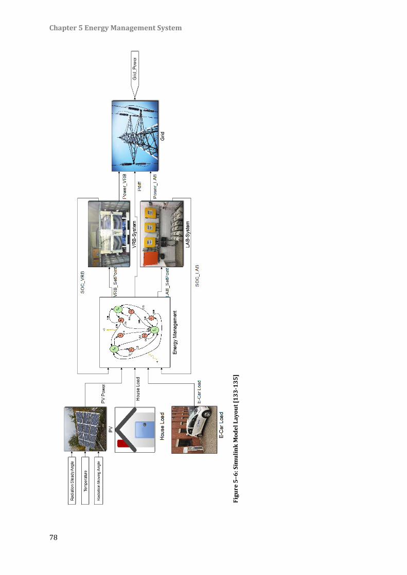
Chapter 5 Energy Management System
78
Fig
ure
5
6: S
imu
lin
k M
od
el
La
yo
ut
[13
3-1
35
]
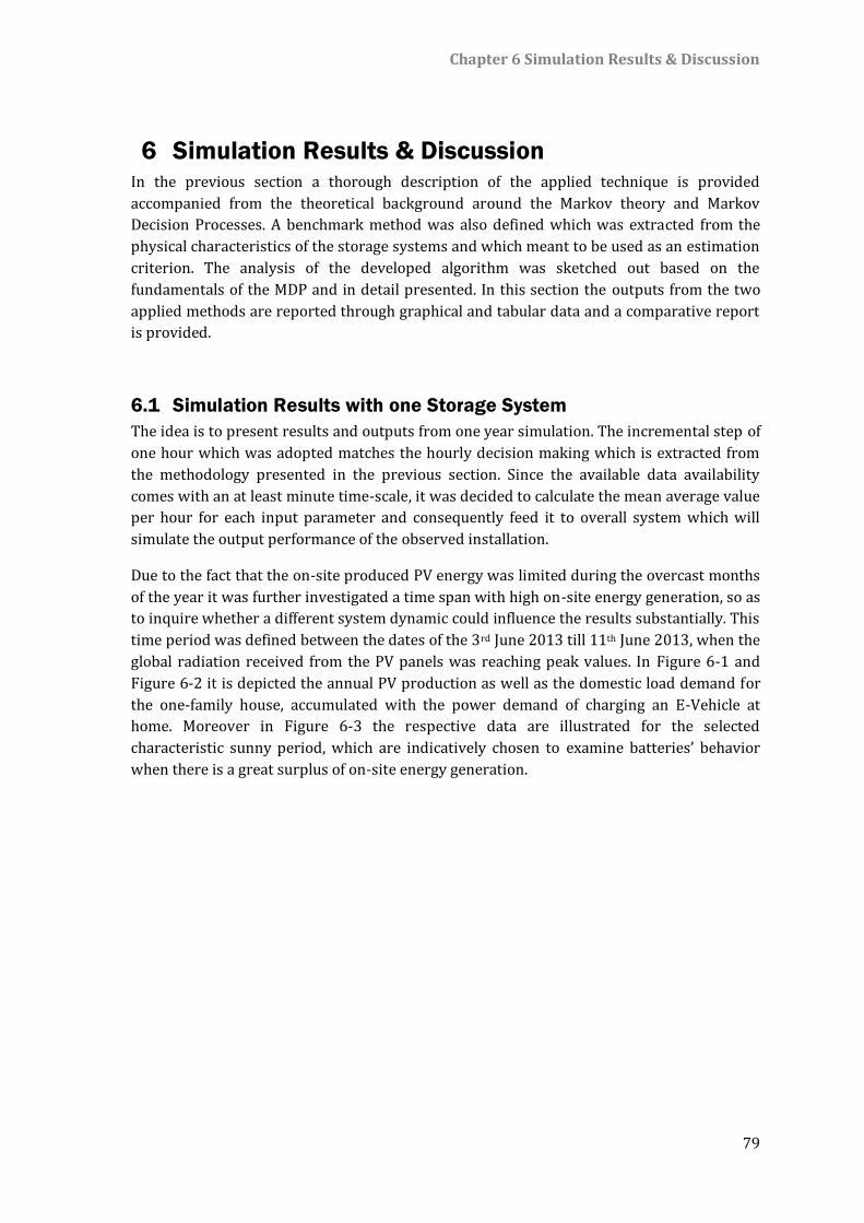
Chapter 6 Simulation Results & Discussion
79
6 Simulation Results & Discussion In the previous section a thorough description of the applied technique is provided
accompanied from the theoretical background around the Markov theory and Markov
Decision Processes. A benchmark method was also defined which was extracted from the
physical characteristics of the storage systems and which meant to be used as an estimation
criterion. The analysis of the developed algorithm was sketched out based on the
fundamentals of the MDP and in detail presented. In this section the outputs from the two
applied methods are reported through graphical and tabular data and a comparative report
is provided.
6.1 Simulation Results with one Storage System
The idea is to present results and outputs from one year simulation. The incremental step of
one hour which was adopted matches the hourly decision making which is extracted from
the methodology presented in the previous section. Since the available data availability
comes with an at least minute time-scale, it was decided to calculate the mean average value
per hour for each input parameter and consequently feed it to overall system which will
simulate the output performance of the observed installation.
Due to the fact that the on-site produced PV energy was limited during the overcast months
of the year it was further investigated a time span with high on-site energy generation, so as
to inquire whether a different system dynamic could influence the results substantially. This
time period was defined between the dates of the 3rd June 2013 till 11th June 2013, when the
global radiation received from the PV panels was reaching peak values. In Figure 6-1 and
Figure 6-2 it is depicted the annual PV production as well as the domestic load demand for
the one-family house, accumulated with the power demand of charging an E-Vehicle at
home. Moreover in Figure 6-3 the respective data are illustrated for the selected
characteristic sunny period, which are indicatively chosen to examine batteries’ behavior
when there is a great surplus of on-site energy generation.
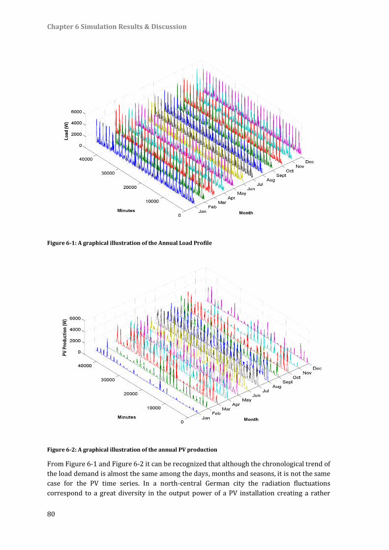
Chapter 6 Simulation Results & Discussion
80
Figure 6-1: A graphical illustration of the Annual Load Profile
Figure 6-2: A graphical illustration of the annual PV production
From Figure 6-1 and Figure 6-2 it can be recognized that although the chronological trend of
the load demand is almost the same among the days, months and seasons, it is not the same
case for the PV time series. In a north-central German city the radiation fluctuations
correspond to a great diversity in the output power of a PV installation creating a rather
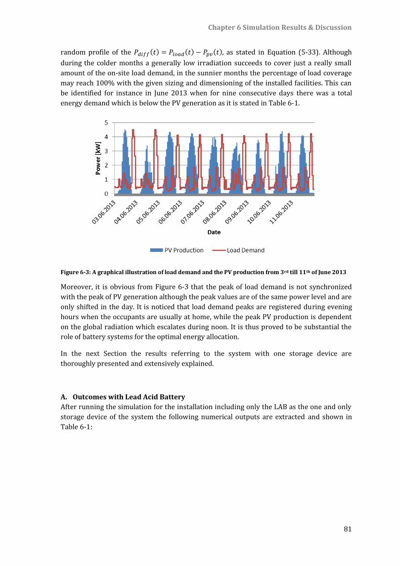
Chapter 6 Simulation Results & Discussion
81
random profile of the 𝑃𝑑𝑖𝑓𝑓(𝑡) = 𝑃𝑙𝑜𝑎𝑑(𝑡) − 𝑃𝑝𝑣(𝑡), as stated in Equation (5-33). Although
during the colder months a generally low irradiation succeeds to cover just a really small
amount of the on-site load demand, in the sunnier months the percentage of load coverage
may reach 100% with the given sizing and dimensioning of the installed facilities. This can
be identified for instance in June 2013 when for nine consecutive days there was a total
energy demand which is below the PV generation as it is stated in Table 6-1.
Figure 6-3: A graphical illustration of load demand and the PV production from 3rd till 11th of June 2013
Moreover, it is obvious from Figure 6-3 that the peak of load demand is not synchronized
with the peak of PV generation although the peak values are of the same power level and are
only shifted in the day. It is noticed that load demand peaks are registered during evening
hours when the occupants are usually at home, while the peak PV production is dependent
on the global radiation which escalates during noon. It is thus proved to be substantial the
role of battery systems for the optimal energy allocation.
In the next Section the results referring to the system with one storage device are
thoroughly presented and extensively explained.
Outcomes with Lead Acid Battery A.
After running the simulation for the installation including only the LAB as the one and only
storage device of the system the following numerical outputs are extracted and shown in
Table 6-1:
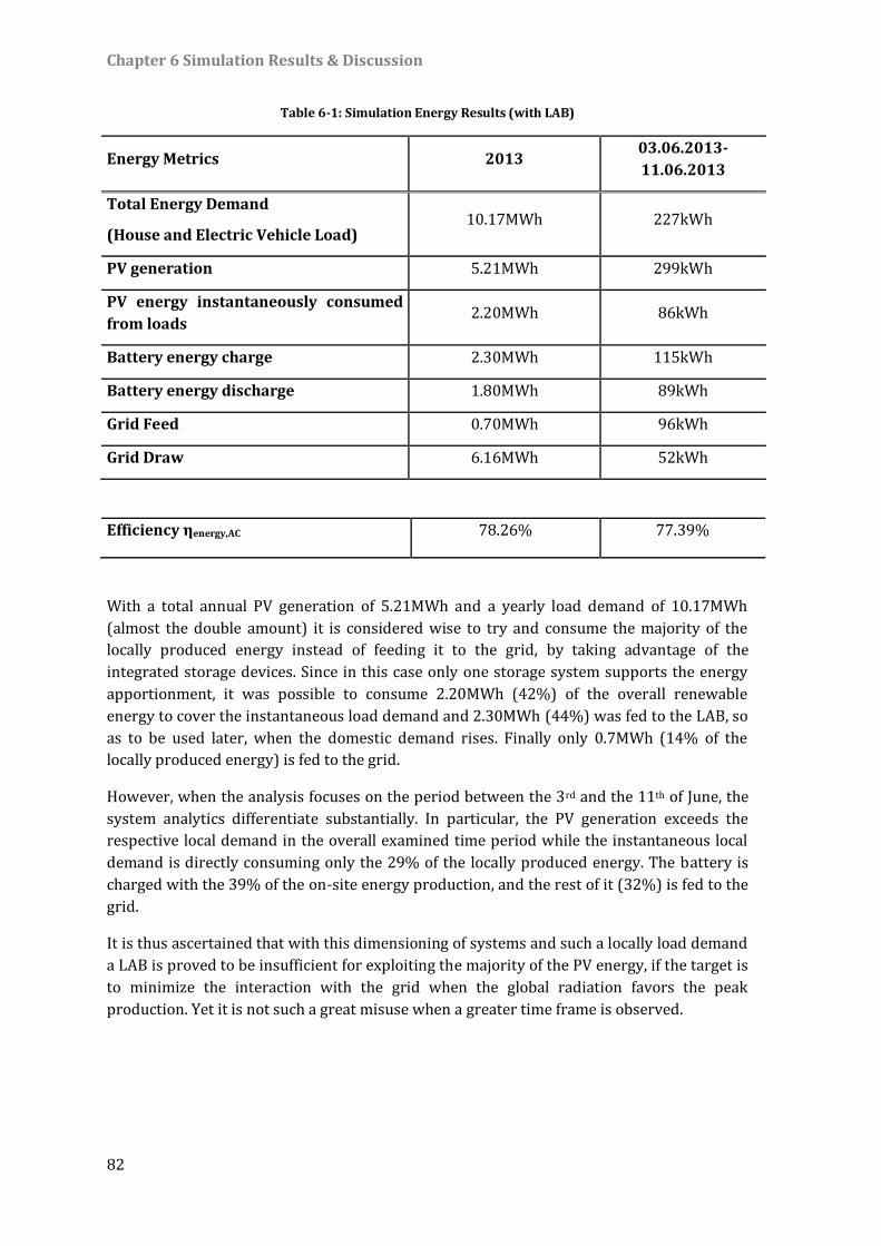
Chapter 6 Simulation Results & Discussion
82
Table 6-1: Simulation Energy Results (with LAB)
Energy Metrics 2013 03.06.2013-
11.06.2013
Total Energy Demand
(House and Electric Vehicle Load) 10.17MWh 227kWh
PV generation 5.21MWh 299kWh
PV energy instantaneously consumed
from loads 2.20MWh 86kWh
Battery energy charge 2.30MWh 115kWh
Battery energy discharge 1.80MWh 89kWh
Grid Feed 0.70MWh 96kWh
Grid Draw 6.16MWh 52kWh
Efficiency ηenergy,AC 78.26% 77.39%
With a total annual PV generation of 5.21MWh and a yearly load demand of 10.17MWh
(almost the double amount) it is considered wise to try and consume the majority of the
locally produced energy instead of feeding it to the grid, by taking advantage of the
integrated storage devices. Since in this case only one storage system supports the energy
apportionment, it was possible to consume 2.20MWh (42%) of the overall renewable
energy to cover the instantaneous load demand and 2.30MWh (44%) was fed to the LAB, so
as to be used later, when the domestic demand rises. Finally only 0.7MWh (14% of the
locally produced energy) is fed to the grid.
However, when the analysis focuses on the period between the 3rd and the 11th of June, the
system analytics differentiate substantially. In particular, the PV generation exceeds the
respective local demand in the overall examined time period while the instantaneous local
demand is directly consuming only the 29% of the locally produced energy. The battery is
charged with the 39% of the on-site energy production, and the rest of it (32%) is fed to the
grid.
It is thus ascertained that with this dimensioning of systems and such a locally load demand
a LAB is proved to be insufficient for exploiting the majority of the PV energy, if the target is
to minimize the interaction with the grid when the global radiation favors the peak
production. Yet it is not such a great misuse when a greater time frame is observed.
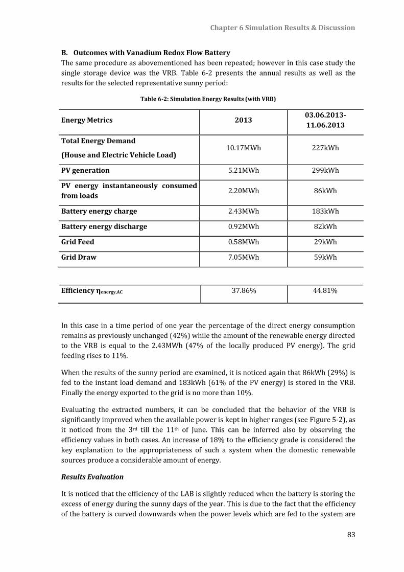
Chapter 6 Simulation Results & Discussion
83
Outcomes with Vanadium Redox Flow Battery B.
The same procedure as abovementioned has been repeated; however in this case study the
single storage device was the VRB. Table 6-2 presents the annual results as well as the
results for the selected representative sunny period:
Table 6-2: Simulation Energy Results (with VRB)
Energy Metrics 2013 03.06.2013-
11.06.2013
Total Energy Demand
(House and Electric Vehicle Load) 10.17MWh 227kWh
PV generation 5.21MWh 299kWh
PV energy instantaneously consumed
from loads 2.20MWh 86kWh
Battery energy charge 2.43MWh 183kWh
Battery energy discharge 0.92MWh 82kWh
Grid Feed 0.58MWh 29kWh
Grid Draw 7.05MWh 59kWh
Efficiency ηenergy,AC 37.86% 44.81%
In this case in a time period of one year the percentage of the direct energy consumption
remains as previously unchanged (42%) while the amount of the renewable energy directed
to the VRB is equal to the 2.43MWh (47% of the locally produced PV energy). The grid
feeding rises to 11%.
When the results of the sunny period are examined, it is noticed again that 86kWh (29%) is
fed to the instant load demand and 183kWh (61% of the PV energy) is stored in the VRB.
Finally the energy exported to the grid is no more than 10%.
Evaluating the extracted numbers, it can be concluded that the behavior of the VRB is
significantly improved when the available power is kept in higher ranges (see Figure 5-2), as
it noticed from the 3rd till the 11th of June. This can be inferred also by observing the
efficiency values in both cases. An increase of 18% to the efficiency grade is considered the
key explanation to the appropriateness of such a system when the domestic renewable
sources produce a considerable amount of energy.
Results Evaluation
It is noticed that the efficiency of the LAB is slightly reduced when the battery is storing the
excess of energy during the sunny days of the year. This is due to the fact that the efficiency
of the battery is curved downwards when the power levels which are fed to the system are
Chapter 6 Simulation Results & Discussion
84
high (see Figure 5-2). Since in the sunny period the produced energy is significantly higher
than in the overcast days, it is realistic that the efficiency ratio drops.
On the contrary the exactly opposite performance is remarked by the VRB. In particular, the
efficiency during higher power rates is elevated and thus the respective losses are
minimized. It is consequently anticipated that the calculated efficiency of the system rises
during sunny days (as it is the selected time frame).
When the grid interaction comes under consideration it is detected that when the LAB is the
only storage device of the examined system then in both case studies the grid export is
higher than that which is attributed to the system with the VRB and the grid import is lower.
This is explained from the efficiency of the storage systems. Although the VRB was capable
of accepting a higher amount of energy in order to reassign it to the loads when needed, its
extended internal power losses are prohibiting the complete reallocation of the stored
energy.
Finally, after a quick glance at the charge and discharge values it is found out that although
the VRB can receive a higher amount of energy than the LAB, due to its narrow efficiency
rate only a smaller percentage of it in comparison to the one delivered from the LAB is
reassigned to the domestic loads. On the other hand the LAB is capable of a higher allocation
rate and in absolute numbers of a higher discharge amount, since the internal losses are not
lavishing the stored energy.
6.2 Simulation Results with Two Storage Systems
After studying the advantages and deficits of the individual battery systems when they
operate as unique storage devices in an one family house, it is time to proceed to the
examination of the combination of storage equipment, in order to create a hybrid system
where the batteries are operating in turn supporting thus the enhancement of the on-site
consumption of the locally produced renewable energy. In the next sections the results for
year simulations as well as for the representative selected sunny period are presented for
the applied control methods, namely the Naive and the Markov based, which are in detail
explained in Section 5.
Outcomes from Naive Approach A.
After combining the two storage systems, simulations for one year and for a sunny period of
nine days are performed while the chosen control algorithm is based on the naive approach
that represents that the optimized outputs will be extracted when the battery system,
namely the LAB, is prioritized against the VRB, which is in any case inferior to the first one.
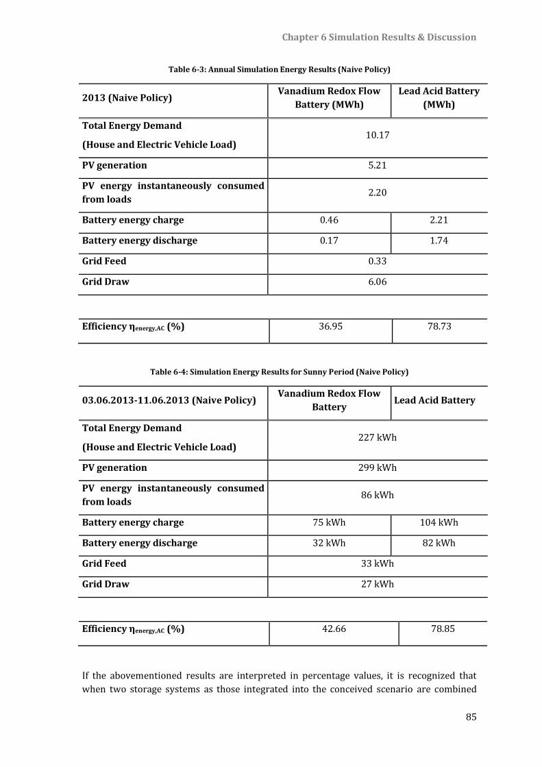
Chapter 6 Simulation Results & Discussion
85
Table 6-3: Annual Simulation Energy Results (Naive Policy)
2013 (Naive Policy) Vanadium Redox Flow
Battery (MWh)
Lead Acid Battery
(MWh)
Total Energy Demand
(House and Electric Vehicle Load) 10.17
PV generation 5.21
PV energy instantaneously consumed
from loads 2.20
Battery energy charge 0.46 2.21
Battery energy discharge 0.17 1.74
Grid Feed 0.33
Grid Draw 6.06
Efficiency ηenergy,AC (%) 36.95 78.73
Table 6-4: Simulation Energy Results for Sunny Period (Naive Policy)
03.06.2013-11.06.2013 (Naive Policy) Vanadium Redox Flow
Battery Lead Acid Battery
Total Energy Demand
(House and Electric Vehicle Load) 227 kWh
PV generation 299 kWh
PV energy instantaneously consumed
from loads 86 kWh
Battery energy charge 75 kWh 104 kWh
Battery energy discharge 32 kWh 82 kWh
Grid Feed 33 kWh
Grid Draw 27 kWh
Efficiency ηenergy,AC (%) 42.66 78.85
If the abovementioned results are interpreted in percentage values, it is recognized that
when two storage systems as those integrated into the conceived scenario are combined
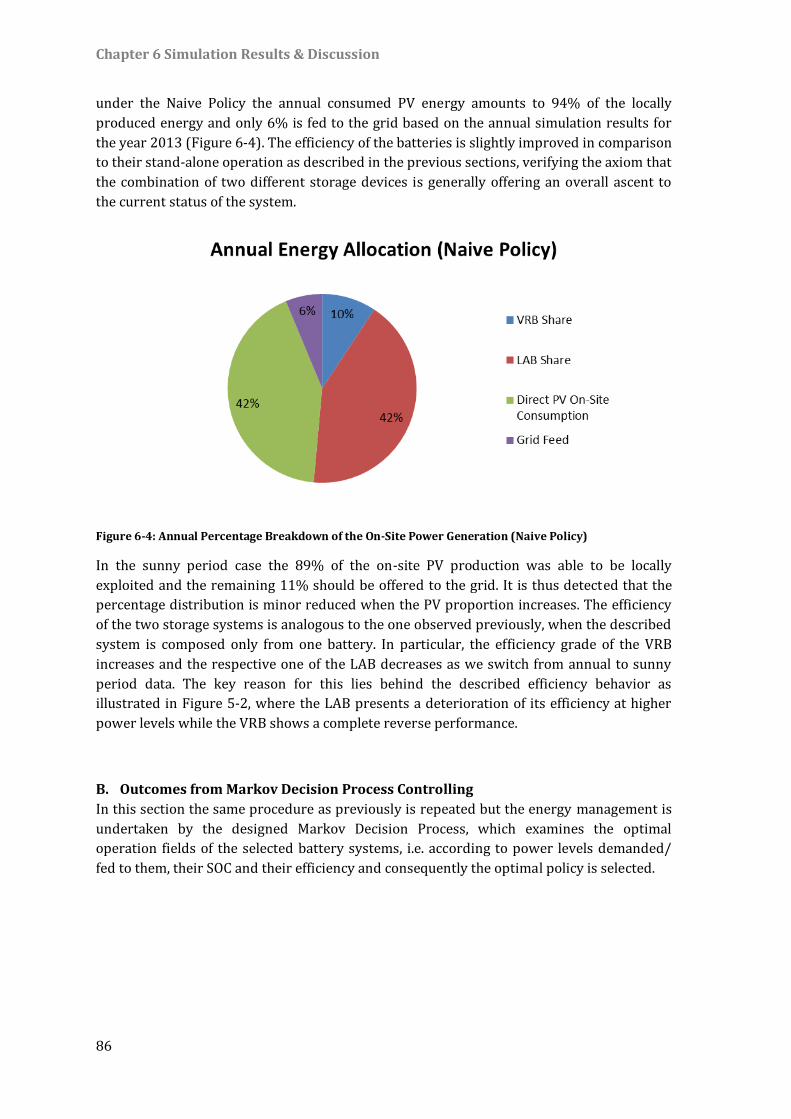
Chapter 6 Simulation Results & Discussion
86
under the Naive Policy the annual consumed PV energy amounts to 94% of the locally
produced energy and only 6% is fed to the grid based on the annual simulation results for
the year 2013 (Figure 6-4). The efficiency of the batteries is slightly improved in comparison
to their stand-alone operation as described in the previous sections, verifying the axiom that
the combination of two different storage devices is generally offering an overall ascent to
the current status of the system.
Figure 6-4: Annual Percentage Breakdown of the On-Site Power Generation (Naive Policy)
In the sunny period case the 89% of the on-site PV production was able to be locally
exploited and the remaining 11% should be offered to the grid. It is thus detected that the
percentage distribution is minor reduced when the PV proportion increases. The efficiency
of the two storage systems is analogous to the one observed previously, when the described
system is composed only from one battery. In particular, the efficiency grade of the VRB
increases and the respective one of the LAB decreases as we switch from annual to sunny
period data. The key reason for this lies behind the described efficiency behavior as
illustrated in Figure 5-2, where the LAB presents a deterioration of its efficiency at higher
power levels while the VRB shows a complete reverse performance.
Outcomes from Markov Decision Process Controlling B.
In this section the same procedure as previously is repeated but the energy management is
undertaken by the designed Markov Decision Process, which examines the optimal
operation fields of the selected battery systems, i.e. according to power levels demanded/
fed to them, their SOC and their efficiency and consequently the optimal policy is selected.
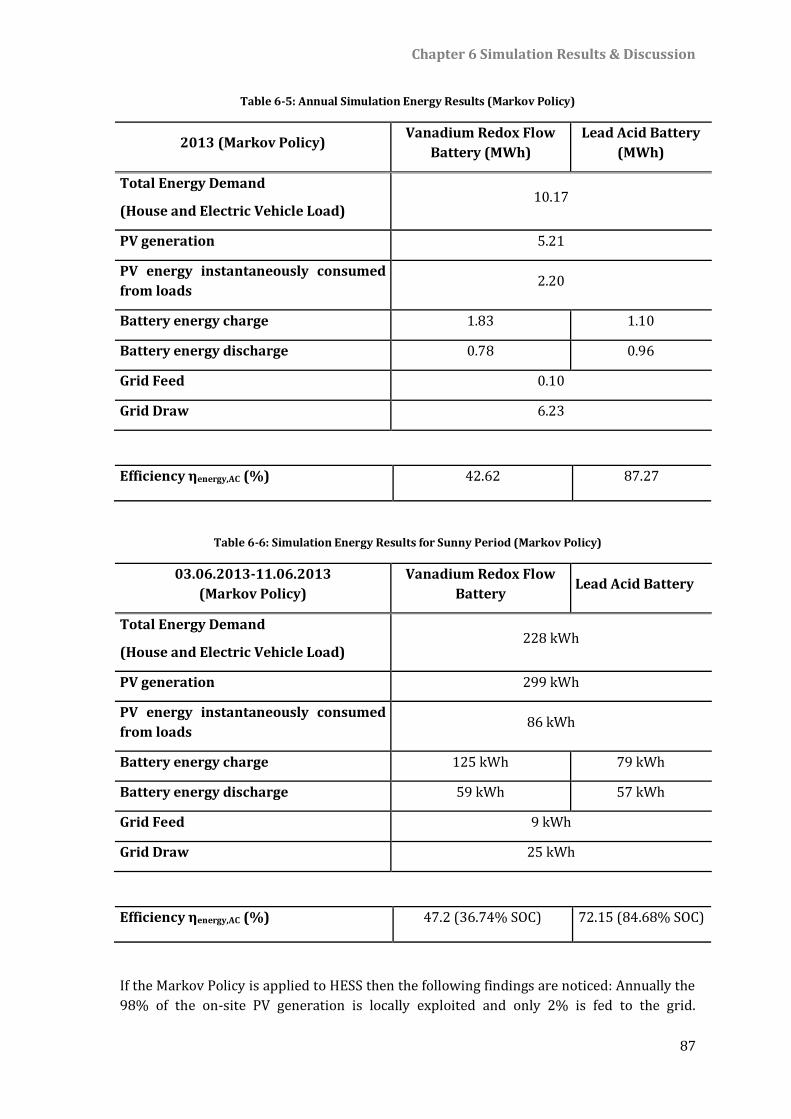
Chapter 6 Simulation Results & Discussion
87
Table 6-5: Annual Simulation Energy Results (Markov Policy)
2013 (Markov Policy) Vanadium Redox Flow
Battery (MWh)
Lead Acid Battery
(MWh)
Total Energy Demand
(House and Electric Vehicle Load) 10.17
PV generation 5.21
PV energy instantaneously consumed
from loads 2.20
Battery energy charge 1.83 1.10
Battery energy discharge 0.78 0.96
Grid Feed 0.10
Grid Draw 6.23
Efficiency ηenergy,AC (%) 42.62 87.27
Table 6-6: Simulation Energy Results for Sunny Period (Markov Policy)
03.06.2013-11.06.2013
(Markov Policy)
Vanadium Redox Flow
Battery Lead Acid Battery
Total Energy Demand
(House and Electric Vehicle Load) 228 kWh
PV generation 299 kWh
PV energy instantaneously consumed
from loads 86 kWh
Battery energy charge 125 kWh 79 kWh
Battery energy discharge 59 kWh 57 kWh
Grid Feed 9 kWh
Grid Draw 25 kWh
Efficiency ηenergy,AC (%) 47.2 (36.74% SOC) 72.15 (84.68% SOC)
If the Markov Policy is applied to HESS then the following findings are noticed: Annually the
98% of the on-site PV generation is locally exploited and only 2% is fed to the grid.
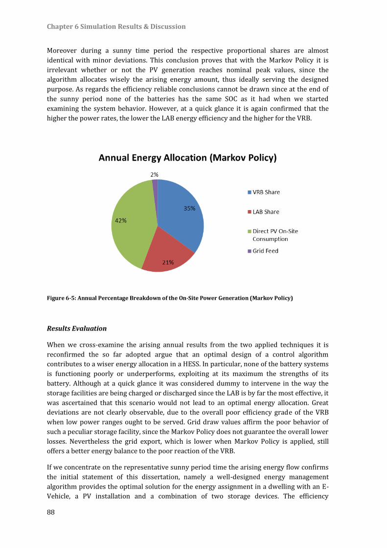
Chapter 6 Simulation Results & Discussion
88
Moreover during a sunny time period the respective proportional shares are almost
identical with minor deviations. This conclusion proves that with the Markov Policy it is
irrelevant whether or not the PV generation reaches nominal peak values, since the
algorithm allocates wisely the arising energy amount, thus ideally serving the designed
purpose. As regards the efficiency reliable conclusions cannot be drawn since at the end of
the sunny period none of the batteries has the same SOC as it had when we started
examining the system behavior. However, at a quick glance it is again confirmed that the
higher the power rates, the lower the LAB energy efficiency and the higher for the VRB.
Figure 6-5: Annual Percentage Breakdown of the On-Site Power Generation (Markov Policy)
Results Evaluation
When we cross-examine the arising annual results from the two applied techniques it is
reconfirmed the so far adopted argue that an optimal design of a control algorithm
contributes to a wiser energy allocation in a HESS. In particular, none of the battery systems
is functioning poorly or underperforms, exploiting at its maximum the strengths of its
battery. Although at a quick glance it was considered dummy to intervene in the way the
storage facilities are being charged or discharged since the LAB is by far the most effective, it
was ascertained that this scenario would not lead to an optimal energy allocation. Great
deviations are not clearly observable, due to the overall poor efficiency grade of the VRB
when low power ranges ought to be served. Grid draw values affirm the poor behavior of
such a peculiar storage facility, since the Markov Policy does not guarantee the overall lower
losses. Nevertheless the grid export, which is lower when Markov Policy is applied, still
offers a better energy balance to the poor reaction of the VRB.
If we concentrate on the representative sunny period time the arising energy flow confirms
the initial statement of this dissertation, namely a well-designed energy management
algorithm provides the optimal solution for the energy assignment in a dwelling with an E-
Vehicle, a PV installation and a combination of two storage devices. The efficiency
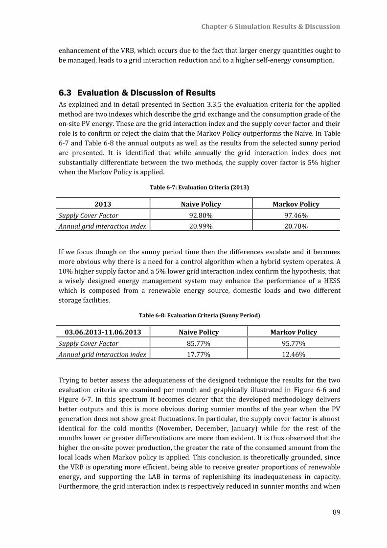
Chapter 6 Simulation Results & Discussion
89
enhancement of the VRB, which occurs due to the fact that larger energy quantities ought to
be managed, leads to a grid interaction reduction and to a higher self-energy consumption.
6.3 Evaluation & Discussion of Results
As explained and in detail presented in Section 3.3.5 the evaluation criteria for the applied
method are two indexes which describe the grid exchange and the consumption grade of the
on-site PV energy. These are the grid interaction index and the supply cover factor and their
role is to confirm or reject the claim that the Markov Policy outperforms the Naive. In Table
6-7 and Table 6-8 the annual outputs as well as the results from the selected sunny period
are presented. It is identified that while annually the grid interaction index does not
substantially differentiate between the two methods, the supply cover factor is 5% higher
when the Markov Policy is applied.
Table 6-7: Evaluation Criteria (2013)
2013 Naive Policy Markov Policy
Supply Cover Factor 92.80% 97.46%
Annual grid interaction index 20.99% 20.78%
If we focus though on the sunny period time then the differences escalate and it becomes
more obvious why there is a need for a control algorithm when a hybrid system operates. A
10% higher supply factor and a 5% lower grid interaction index confirm the hypothesis, that
a wisely designed energy management system may enhance the performance of a HESS
which is composed from a renewable energy source, domestic loads and two different
storage facilities.
Table 6-8: Evaluation Criteria (Sunny Period)
03.06.2013-11.06.2013 Naive Policy Markov Policy
Supply Cover Factor 85.77% 95.77%
Annual grid interaction index 17.77% 12.46%
Trying to better assess the adequateness of the designed technique the results for the two
evaluation criteria are examined per month and graphically illustrated in Figure 6-6 and
Figure 6-7. In this spectrum it becomes clearer that the developed methodology delivers
better outputs and this is more obvious during sunnier months of the year when the PV
generation does not show great fluctuations. In particular, the supply cover factor is almost
identical for the cold months (November, December, January) while for the rest of the
months lower or greater differentiations are more than evident. It is thus observed that the
higher the on-site power production, the greater the rate of the consumed amount from the
local loads when Markov policy is applied. This conclusion is theoretically grounded, since
the VRB is operating more efficient, being able to receive greater proportions of renewable
energy, and supporting the LAB in terms of replenishing its inadequateness in capacity.
Furthermore, the grid interaction index is respectively reduced in sunnier months and when
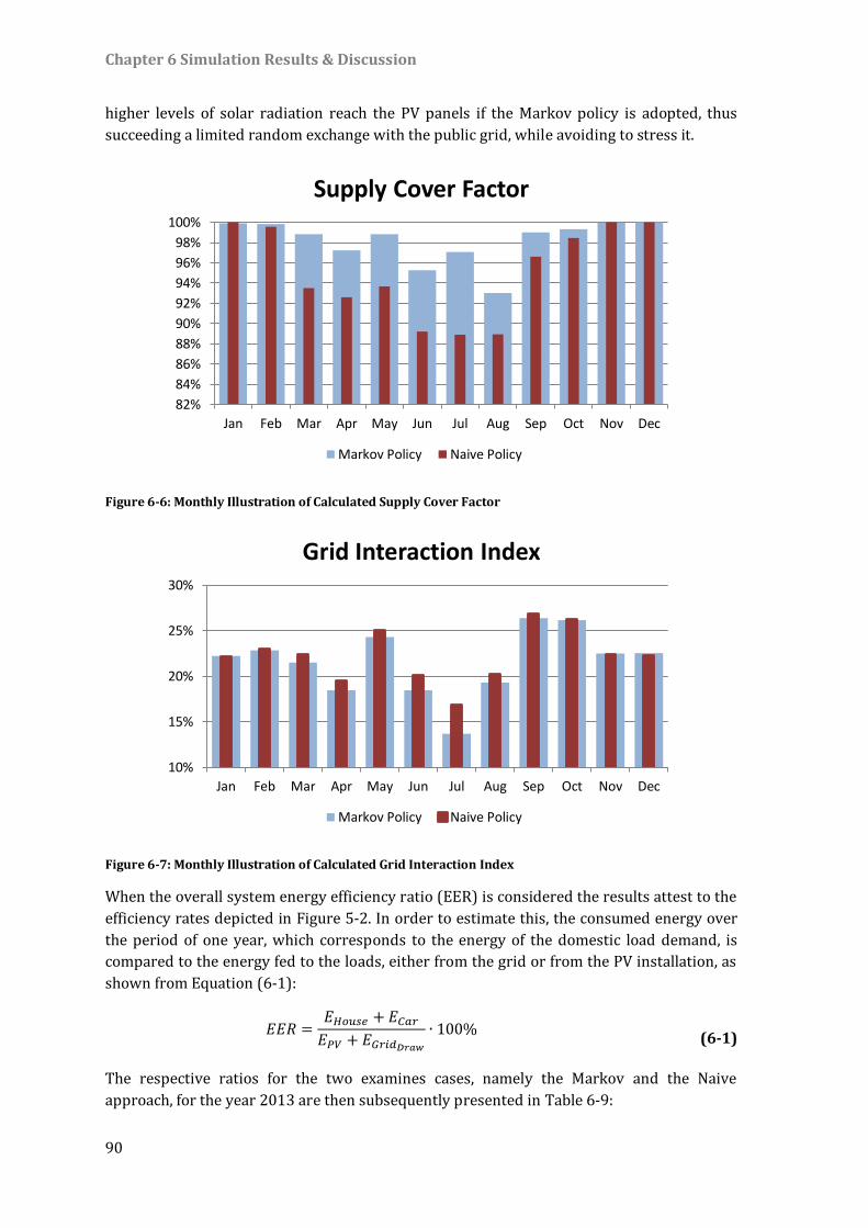
Chapter 6 Simulation Results & Discussion
90
higher levels of solar radiation reach the PV panels if the Markov policy is adopted, thus
succeeding a limited random exchange with the public grid, while avoiding to stress it.
Figure 6-6: Monthly Illustration of Calculated Supply Cover Factor
Figure 6-7: Monthly Illustration of Calculated Grid Interaction Index
When the overall system energy efficiency ratio (EER) is considered the results attest to the
efficiency rates depicted in Figure 5-2. In order to estimate this, the consumed energy over
the period of one year, which corresponds to the energy of the domestic load demand, is
compared to the energy fed to the loads, either from the grid or from the PV installation, as
shown from Equation (6-1):
𝐸𝐸𝑅 =𝐸𝐻𝑜𝑢𝑠𝑒 + 𝐸𝐶𝑎𝑟𝐸𝑃𝑉 + 𝐸𝐺𝑟𝑖𝑑𝐷𝑟𝑎𝑤
∙ 100% (6-1)
The respective ratios for the two examines cases, namely the Markov and the Naive
approach, for the year 2013 are then subsequently presented in Table 6-9:
82%
84%
86%
88%
90%
92%
94%
96%
98%
100%
Jan Feb Mar Apr May Jun Jul Aug Sep Oct Nov Dec
Supply Cover Factor
Markov Policy Naive Policy
10%
15%
20%
25%
30%
Jan Feb Mar Apr May Jun Jul Aug Sep Oct Nov Dec
Grid Interaction Index
Markov Policy Naive Policy
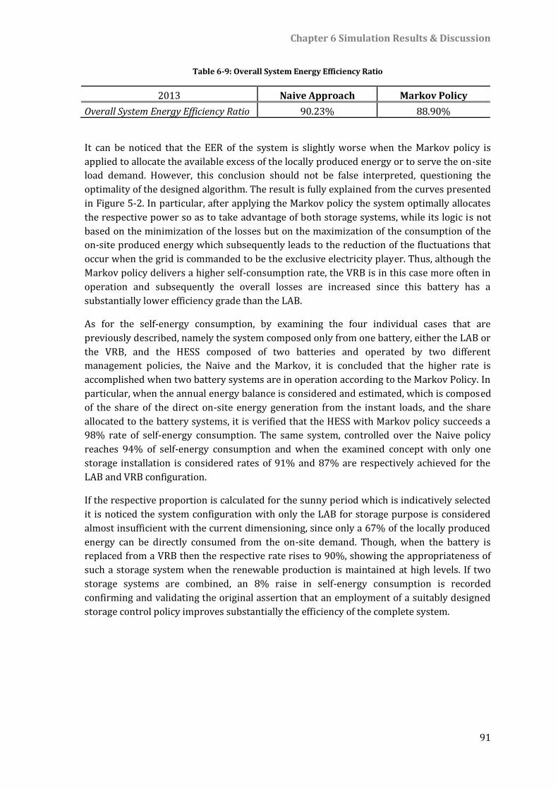
Chapter 6 Simulation Results & Discussion
91
Table 6-9: Overall System Energy Efficiency Ratio
2013 Naive Approach Markov Policy
Overall System Energy Efficiency Ratio 90.23% 88.90%
It can be noticed that the EER of the system is slightly worse when the Markov policy is
applied to allocate the available excess of the locally produced energy or to serve the on-site
load demand. However, this conclusion should not be false interpreted, questioning the
optimality of the designed algorithm. The result is fully explained from the curves presented
in Figure 5-2. In particular, after applying the Markov policy the system optimally allocates
the respective power so as to take advantage of both storage systems, while its logic is not
based on the minimization of the losses but on the maximization of the consumption of the
on-site produced energy which subsequently leads to the reduction of the fluctuations that
occur when the grid is commanded to be the exclusive electricity player. Thus, although the
Markov policy delivers a higher self-consumption rate, the VRB is in this case more often in
operation and subsequently the overall losses are increased since this battery has a
substantially lower efficiency grade than the LAB.
As for the self-energy consumption, by examining the four individual cases that are
previously described, namely the system composed only from one battery, either the LAB or
the VRB, and the HESS composed of two batteries and operated by two different
management policies, the Naive and the Markov, it is concluded that the higher rate is
accomplished when two battery systems are in operation according to the Markov Policy. In
particular, when the annual energy balance is considered and estimated, which is composed
of the share of the direct on-site energy generation from the instant loads, and the share
allocated to the battery systems, it is verified that the HESS with Markov policy succeeds a
98% rate of self-energy consumption. The same system, controlled over the Naive policy
reaches 94% of self-energy consumption and when the examined concept with only one
storage installation is considered rates of 91% and 87% are respectively achieved for the
LAB and VRB configuration.
If the respective proportion is calculated for the sunny period which is indicatively selected
it is noticed the system configuration with only the LAB for storage purpose is considered
almost insufficient with the current dimensioning, since only a 67% of the locally produced
energy can be directly consumed from the on-site demand. Though, when the battery is
replaced from a VRB then the respective rate rises to 90%, showing the appropriateness of
such a storage system when the renewable production is maintained at high levels. If two
storage systems are combined, an 8% raise in self-energy consumption is recorded
confirming and validating the original assertion that an employment of a suitably designed
storage control policy improves substantially the efficiency of the complete system.
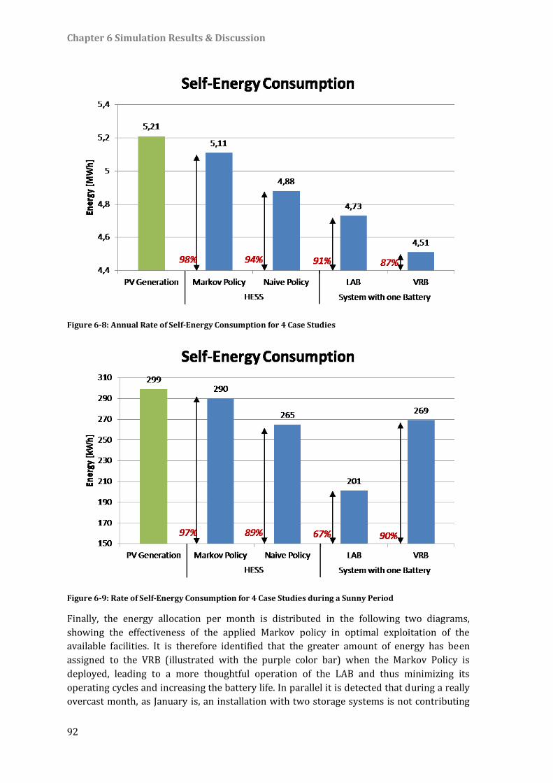
Chapter 6 Simulation Results & Discussion
92
Figure 6-8: Annual Rate of Self-Energy Consumption for 4 Case Studies
Figure 6-9: Rate of Self-Energy Consumption for 4 Case Studies during a Sunny Period
Finally, the energy allocation per month is distributed in the following two diagrams,
showing the effectiveness of the applied Markov policy in optimal exploitation of the
available facilities. It is therefore identified that the greater amount of energy has been
assigned to the VRB (illustrated with the purple color bar) when the Markov Policy is
deployed, leading to a more thoughtful operation of the LAB and thus minimizing its
operating cycles and increasing the battery life. In parallel it is detected that during a really
overcast month, as January is, an installation with two storage systems is not contributing
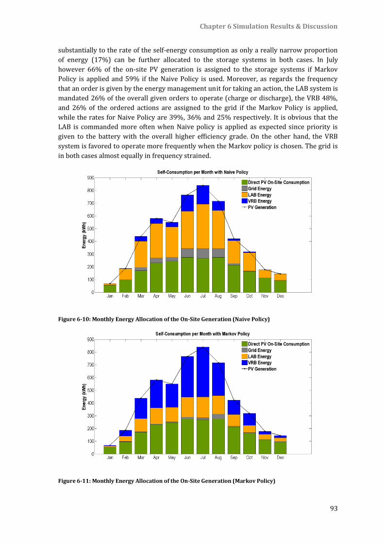
Chapter 6 Simulation Results & Discussion
93
substantially to the rate of the self-energy consumption as only a really narrow proportion
of energy (17%) can be further allocated to the storage systems in both cases. In July
however 66% of the on-site PV generation is assigned to the storage systems if Markov
Policy is applied and 59% if the Naive Policy is used. Moreover, as regards the frequency
that an order is given by the energy management unit for taking an action, the LAB system is
mandated 26% of the overall given orders to operate (charge or discharge), the VRB 48%,
and 26% of the ordered actions are assigned to the grid if the Markov Policy is applied,
while the rates for Naive Policy are 39%, 36% and 25% respectively. It is obvious that the
LAB is commanded more often when Naive policy is applied as expected since priority is
given to the battery with the overall higher efficiency grade. On the other hand, the VRB
system is favored to operate more frequently when the Markov policy is chosen. The grid is
in both cases almost equally in frequency strained.
Figure 6-10: Monthly Energy Allocation of the On-Site Generation (Naive Policy)
Figure 6-11: Monthly Energy Allocation of the On-Site Generation (Markov Policy)

Chapter 6 Simulation Results & Discussion
94
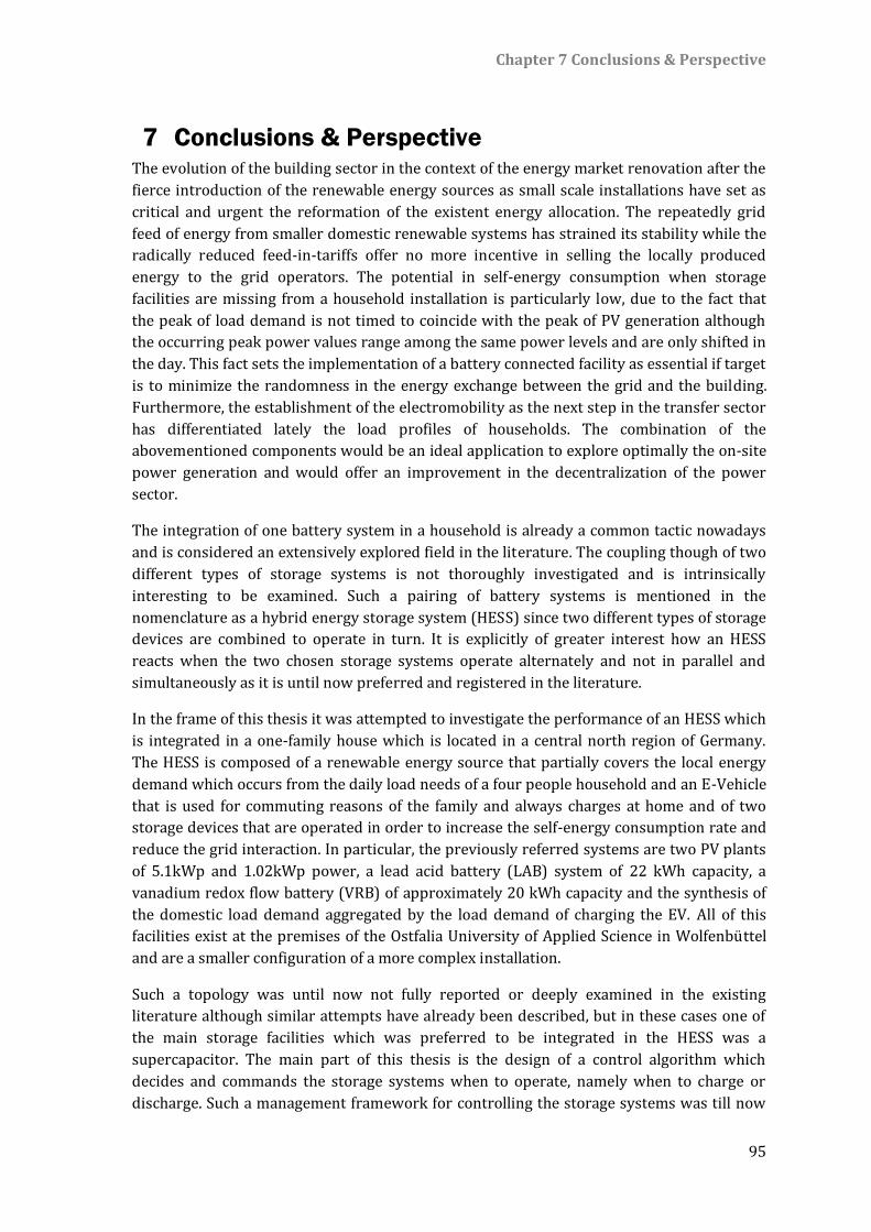
Chapter 7 Conclusions & Perspective
95
7 Conclusions & Perspective The evolution of the building sector in the context of the energy market renovation after the
fierce introduction of the renewable energy sources as small scale installations have set as
critical and urgent the reformation of the existent energy allocation. The repeatedly grid
feed of energy from smaller domestic renewable systems has strained its stability while the
radically reduced feed-in-tariffs offer no more incentive in selling the locally produced
energy to the grid operators. The potential in self-energy consumption when storage
facilities are missing from a household installation is particularly low, due to the fact that
the peak of load demand is not timed to coincide with the peak of PV generation although
the occurring peak power values range among the same power levels and are only shifted in
the day. This fact sets the implementation of a battery connected facility as essential if target
is to minimize the randomness in the energy exchange between the grid and the building.
Furthermore, the establishment of the electromobility as the next step in the transfer sector
has differentiated lately the load profiles of households. The combination of the
abovementioned components would be an ideal application to explore optimally the on-site
power generation and would offer an improvement in the decentralization of the power
sector.
The integration of one battery system in a household is already a common tactic nowadays
and is considered an extensively explored field in the literature. The coupling though of two
different types of storage systems is not thoroughly investigated and is intrinsically
interesting to be examined. Such a pairing of battery systems is mentioned in the
nomenclature as a hybrid energy storage system (HESS) since two different types of storage
devices are combined to operate in turn. It is explicitly of greater interest how an HESS
reacts when the two chosen storage systems operate alternately and not in parallel and
simultaneously as it is until now preferred and registered in the literature.
In the frame of this thesis it was attempted to investigate the performance of an HESS which
is integrated in a one-family house which is located in a central north region of Germany.
The HESS is composed of a renewable energy source that partially covers the local energy
demand which occurs from the daily load needs of a four people household and an E-Vehicle
that is used for commuting reasons of the family and always charges at home and of two
storage devices that are operated in order to increase the self-energy consumption rate and
reduce the grid interaction. In particular, the previously referred systems are two PV plants
of 5.1kWp and 1.02kWp power, a lead acid battery (LAB) system of 22 kWh capacity, a
vanadium redox flow battery (VRB) of approximately 20 kWh capacity and the synthesis of
the domestic load demand aggregated by the load demand of charging the EV. All of this
facilities exist at the premises of the Ostfalia University of Applied Science in Wolfenbüttel
and are a smaller configuration of a more complex installation.
Such a topology was until now not fully reported or deeply examined in the existing
literature although similar attempts have already been described, but in these cases one of
the main storage facilities which was preferred to be integrated in the HESS was a
supercapacitor. The main part of this thesis is the design of a control algorithm which
decides and commands the storage systems when to operate, namely when to charge or
discharge. Such a management framework for controlling the storage systems was till now
Chapter 7 Conclusions & Perspective
96
trivially explored while the various techniques that were applied were not appropriate for a
solution approach for the designed case study. In this thesis, the advantages of a combined
VRB/LAB storage facility in the domestic field were detailed reported and the performance
of such an HESS was also juxtaposed to simpler syntheses, where only one storage device
was each time available.
Consecutively, the main research question which was addressed has been formulated as
follows:
“How can the energy flow in a single-family house be managed efficiently, so as to
maximize the self-consumption of the produced renewable energy and minimize the grid
interaction by controlling two different stationary storage systems?”
So as to handle and in detail examine the primary research problematic three further
subquestions had to be tackled and analysed. These referred to the identification of the
appropriate models to represent precisely the existing facilities, the detection of the optimal
method to be applied in order to implement the selected energy management policy so as to
control the charging and discharging process of two stationary storage systems and
ultimately the evaluation of the designed technique.
In particular, these are formulated as follows:
“Which are the appropriate models to represent the existing facilities?”
“Which method is optimal to be applied in order to implement the selected energy
management policy so as to control the charging and discharging process of two
stationary storage systems?”
“How can the chosen technique be evaluated?”
In the whole process great importance has been attached to the plausibility of the input and
extracted data, by applying the management algorithm on a designed block of models which
represents precisely the operation of the abovementioned facilities, that are physically also
integrated in the Energy Park of the Ostfalia University. These models were conceived and
created in the Matlab/ Simulink environment and a joint block system was generated. With
models that are explicitly designed to depict the exact performance of real devices, but
incorporating also the generalization factor, it was prevented to create an ideal system with
null losses that most of the case studies apply in the literature. On the contrary, the system
operation is fully analogous to the exact devices of the utilized test bed, which nevertheless
correspond to a great variety of the existing market available and commercially mature
systems.
The main research topic which was handled in the current study was the development of
the energy management system which would be considered a strategic approach to charge
and discharge the given battery systems in an optimal and efficient way. The choice of the
appropriate management technique emerged from an extensive literature review and from
the dynamic inputs that were to be integrated in its logic, according to the degree of
influence they had on the extracted decision output. It has been advocated that the control
policy should be based on the Markov Decision Process, a technique stemming from the
reinforcement learning field which is commonly used to solve problems with stochastic
dynamics. This method is also appropriate for problems which require a decision making at
Chapter 7 Conclusions & Perspective
97
regular time intervals as in the examined case study. The main integrated variables that
were considered in the design process regarded the power difference between the instant
on-site PV power generation and the direct load demand, the SOC of the storage devices and
the efficiency of these at the respective power levels. The described method was designed in
such a way that would also be applicable in any other hybrid storage system where the
efficiencies of the batteries are not considered constant, though they are dependent on the
SOC and the power and are in advance known, while the financial aspect was neglected.
So as to evaluate the extracted outputs a benchmark method had been applied, which is
based on the performance of the two storage devices, namely their efficiency grade under
various charge/discharge power levels. In addition, the comparative metrics which were
computed for the designed and the benchmark method are two factors which are related to
the self-energy consumption and the grid interaction, i. e. the supply cover factor and the
grid interaction index.
The simulation process included the examination of two research periods. The first one is
the reference year 2013 and real registered data of temperature, global radiation and cloud
factor were used as input so as to acquire a plausible depiction of the conceived scenario.
Due to the fact that the PV generation remains limited for an extended time span during a
year in the examined region it was decided to examine system’s behavior and performance
for an indicative sunny period. In this framework nine consecutive sunny days (from the 3rd
until the 11th of June 2013) were selected and the simulation process was repeated.
In addition the observed case studies were divided into two categories; the first referred to
a system with only one storage system as backup solution and the second referred to the
complete HESS as it was initially presented. Target was to compare the appropriateness of
the two arrangements as well as to evaluate how far a control technique may improve the
performance of an HESS.
In the one battery system topology, if the chosen battery was the LAB system 86% of the
locally produced energy was consumed locally in the time frame of one year whereas when
the VRB was the one only storage device of the system the overall self-energy consumption
rose to 89%. The respective proportions for the sunny period were 68% and 90%. It is
obvious that the LAB is sufficiently scaled for long-term use, though when the same concept
would be transferred in a sunnier region this storage device would be inadequate. On the
contrary the VRB operates in such a way that allows almost the equal percentage of self-
energy consumption regardless of the on-site energy generation.
When the complete HESS was considered, there was an increase in these ratios since a
higher capacity offered a higher flexibility to the allocation mechanism. The application of
the Naive policy which is related to the benchmark method, and is extracted from the
efficiency of the two storage devices, yielded a renewable energy consumption of 94%.
When though the control technique designed according the Markov Decision Process theory
is preferred then the respective annual ratio rose to 98%. Under high global radiation
circumstances (during the selected sunny period time) the percentage dropped to 89% for
the Naive policy while for the designed Markov technique remained unaffected. It is thus
proved the superiority of the applied method towards a trivial approach and the necessity of
Chapter 7 Conclusions & Perspective
98
a control strategy so as to succeed a high degree of optimal use of the considered storage
devices.
The juxtaposing of the two case studies (the one storage system case and the HESS)
illustrated also the weakness of a stand-alone LAB to support such a synthesis of loads and
decentralized production when there is increased on-site generation, while the VRB system
proved to be more flexible, even in the domestic field in which is not yet extensively
employed.
In addition, the calculation of the evaluation criteria which were the two factors that
depicted the self-energy consumption and the grid interaction support the initial claim that
two different storage devices which must operate in turn to serve the same domestic
installation, should be externally controlled in order to fully utilize their attributes. For both
the annual and the sunny period results it is determined that an intelligent designed
algorithm offers a better exploitation of the self-produced energy, since a higher score in
self-energy consumption is accomplished while the grid interaction is reduced.
Future Work
Although the complete mechanism has been tested and simulated with input data, that
represent to a great extent the real demand, generation and responses of the individual
components, it would be of great interest if the designed architecture could be additionally
tested in the real facilities so as to further examine the plausibility of the simulated results.
The integration of the examined concept and control technique in the context of a project
would offer valuable information on the suitability of the designed method and would reveal
perhaps unconsidered aspects.
In addition a sensitivity analysis of succeeding an ideal scaling of all the facilities analogous
to the needs of the domestic load demand could be also proved significant for extracting
conclusions for topologies with the same morphology but with different sizing. However in
this case, a possible theoretical scaling of the integrated components of the system may
involve risks and may end up to a misleading output, since it is possible that not all the
considered parameters are allowed to be respectively scaled. Nevertheless, an analysis in a
practical context and a juxtaposition of the outcomes would be meaningful and is open for
future research.
References
99
References 1. European Commission. European Climate Change Programme, EU Action, European
Commission. Link: http://ec.europa.eu/clima/policies/eccp/index_en.htm,
2. The National People’s Congress of the People’s Republic of China. The Renewable
Energy Law of the People’s Republic of China. 2009. Link:
http://www.npc.gov.cn/englishnpc/Special/CombatingClimateChange/2009-
08/25/content_1515301.htm
3. Bundesministerium für Wirtschaft und Energie (BMWi). Die Energie der Zukunft,
Erster Fortschrittsbericht zur Energiewende, Bundesministerium für Wirtschaft
und Energie (BMWi), Berlin, Germany, December 2014.
4. International Energy Agency. Transition to Sustainable Buildings Strategies and
Opportunities to 2050, OECD/IEA, Paris, France, 2013.
5. D. Ürge-Vorsatz, N. Eyre, P. Graham, D. Harvey, E. Hertwich, Y. Jiang, C. Kornevall, M.
Majumdar, J. E. McMahon, S. Mirasgedis, S. Murakami, A. Novikova. Energy End-
Use: Building. In Global Energy Assessment - Toward a Sustainable Future,
Cambridge University Press, Cambridge, UK and New York, NY, USA and the
International Institute for Applied Systems Analysis, Laxenburg, Austria, pp. 649-
760, 2012.
6. German Solar Industry Association (BSW-Solar). Statistische Zahlen der deutschen
Solarstrombranche (Photovoltaik), German Solar Industry Association (BSW-
Solar), June 2015.
7. Bundesministeriums der Justiz und für Verbraucherschutz. Gesetz für den Ausbau
erneuerbarer Energien (Erneuerbare-Energien-Gesetz - EEG 2014),
Bundesministeriums der Justiz und für Verbraucherschutz, Juli 2014 (BGBl. I S.
1066).
8. Degressions- und Vergütungssätze Juli bis September 2016, Bundesnetzagentur,
Stand: 31.08.2016. Link:
http://www.bundesnetzagentur.de/cln_1431/DE/Sachgebiete/ElektrizitaetundG
as/Unternehmen_Institutionen/ErneuerbareEnergien/Photovoltaik/DatenMeldg
n_EEG-VergSaetze/DatenMeldgn_EEG-
VergSaetze_node.html;jsessionid=E8E8B4B4BD2F6A92322C2480D76BE3B8#do
c405794bodyText4
9. C. Kost, J. N. Mayer, J. Thomsen, N. Hartmann, C. Senkpiel, S. Philipps, S. Nold, S. Lude,
T. Schlegl. Stromgestehungskosten Erneuerbare Energien Studie, Fraunhofer-
Institut für Solare Energiesysteme ISE, Freiburg, Germany, November 2013.
10. J. Weniger, T. Tjaden, V. Quaschning. Solare Unabhängigkeitserklärung, Photovoltaik,
Oktober 2012
11. H. Wirth. Recent Facts about Photovoltaics in Germany, Fraunhofer ISE, Freiburg,
Germany, 2016.
12. Bundesverband Solarwirtschaft. Infos zur neuen förderung von Solarstrom –
Speichern, Informationspapier des BSW-Solar, Bundesverband Solarwirtschaft.
Stand: 29.2.2016.
13. Bundesministerium für Umwelt, Naturschutz, Bau und Reaktorsicherheit – BMUB.
Kurzinfo Elektromobilität, BMUB, Stand: 28.09.2016. Link:
www.bmub.bund.de/P706/
References
100
14. K.P. Kairies, D. Haberschusz, J. v. O., J. Strebel, O. Wessels, D. Magnor, J. Badeda, D. U.
Sauer. Jahresbericht zum Speichermonitoring entstand im Rahmen des
Forschungsvorhabens Wissenschaftliches Mess¬ und Evaluierungsprogramm
Solarstromspeicher (WMEP PV¬Speicher), Institut für Stromrichtertechnik und
Elektrische Antriebe der RWTH, Aachen, 2016.
15. C. Daniel, J. O. Besenhard. Handbook of Battery Materials, 2. ed. Wiley-VCH Verlag
GmbH & Co. KGaA., Weinheim, Germany, 2011.
16. E. Jimenez. Resource Allocation And Load-Shedding Policies Based On Markov
Decision Processes For Renewable Energy Generation And Storage, Master
Thesis, University of Central Florida, Orlando, Florida, USA, 2015.
17. X. Qiu. Modeling and optimization of energy storage system for microgrid, PhD
Thesis, Missouri University of Science and Technology, Missouri, USA, 2014.
18. L. Baumann. Improved System Models for Building-Integrated Hybrid Renewable
Energy Systems with Advanced Storage: A Combined Experimental and
Simulation Approach, PhD Thesis, De Montfort University, Leicester, UK, 2015.
19. P. Stenzel, J. Linssen, J. Fleer. Impact of Different Load Profiles on Cost Optimal
System Designs for Battery Supported PV Systems, presented in the 7th
International Conference on Applied Energy – ICAE2015, Energy Procedia 75,
1862 – 1868, 2015.
20. J. Dickert, T. Heß, P. Schegner, C. Felsmann. Electrical Design of an Efficiency House
Plus, presented in the 3rd IEEE PES Innovative Smart Grid Technologies Europe
(ISGT Europe), Berlin, Germany, 2012.
21. R. Bellman. A Markovian decision process, Journal of Mathematical Mechanics, 6 (5),
pp. 679–684, 1957.
22. C. Guan, Y. Wang, X. Lin, S. Nazarian, M. Pedram. Reinforcement Learning-Based
Control of Residential Energy Storage Systems for Electric Bill Minimization,
Consumer Communications and Networking Conference (CCNC), 12th Annual
IEEE, Date of Conference: 9-12 Jan. 2015, IEEE, 2015.
23. E. Boggasch, M. Heiser, R.D. Patzelt. Busgestütztes Energiemanagement eines
Verbundes regenerativer Energieanlagen am Institut für Verbrennungstechnik
und Prozessautomation an der Fachhochschule Braunschweig/Wolfenbüttel,
AGIP-Forschungsvorhaben F.A.-Nr. 2003.525 Report, Wolfenbüttel, Germany,
2006.
24. Strom-Report. Photovoltaik in Deutschland, Link: www.Strom-Report.de.
25. Bundesministerium für Wirtschaft und Energie (BMWi). Zeitreihen zur Entwicklung
der erneuerbaren Energien in Deutschland unter Verwendung von Daten der
Arbeitsgruppe Erneuerbare Energien-Statistik (AGEE-Stat) (Stand: August 2016),
BMWi, Berlin, Germany.
26. K. Schneider. Low-cost wafers for solar cells, Research News / 1.10.2015, Fraunhofer
Institute for Solar Energy Systems ISE, Freiburg, Germany, 2015.
27. Photon International. Entwicklung der mittleren Wirkungsgrade von PV-Module auf
Basis von mono- und multikristallinen Zellen nach dem Jahr der Markteinführung,
Daten aus Photon International 2014-02.
28. Kelly Pickerel. What are the different types of solar modules?, Solar Power World,
July 2015, Link: https://www.solarpowerworldonline.com/2015/07/what-are-
the-different-types-of-solar-modules/
References
101
29. Energie-Experten. Wirkungsgrad von Solarmodulen im Vergleich, Link:
http://www.energie-experten.org/erneuerbare-
energien/photovoltaik/solarmodule/wirkungsgrad.html
30. C. F. Gay, J.H. Wilson, J.W. Yerkes. Performance advantages of two-axis tracking for
large flat-plate photovoltaic energy systems, in: Photovoltaic Specialists
Conference, 16th, San Diego, CA, USA, September 27-30, 1982, New York, Institute
of Electrical and Electronics Engineers, pp. 1368-1371, 1982
31. D.L. King, W.E. Boyson, J.A. Kratochvil. Analysis of factors influencing the annual
energy production of photovoltaic systems, Photovoltaic Specialists Conference,
2002, Conference Record of the Twenty-Ninth IEEE: pp. 1356–1361, 2002.
32. SMA Regelsysteme GmbH. Sunny Boy 2000, Technische Beschreibung, SMA
Regelsysteme GmbH, 2000.
33. SMA Solar Technology AG. Sunny Boy 1200, Installationsanleitung, SMA Solar
Technology AG, 2000.
34. X. H. Nguyen, M. P. Nguyen. Mathematical modeling of photovoltaic
cell/module/arrays with tags in Matlab/Simulink, Environmental Systems
Research 4:24, 2015.
35. T. Glotzbach. Ein Beitrag zur mathematischen Charakterisierung von Photovoltaik-
Dünnschichttechnologien auf Basis realer I/U-Kennlinien, Ph.D Thesis, Kassel
University Press, Kassel, Germany, December 2010.
36. D. Rekioua, E. Matagne. Modeling of Solar Irradiance and Cells, Optimization of
Photovoltaic Power Systems, Chapter 2 of Green Energy and Technology,
Springer-Verlag, London, UK, 2012.
37. K. Nishioka, N. Sakitani, Y. Uraoka, T. Fuyuki. Analysis of multicrystalline silicon solar
cells by modified 3-diode equivalent circuit model taking leakage current through
periphery into consideration, Solar Energy Materials and Solar Cells, 91, pp.
1222–1227, 2007.
38. J. A. Gow, C. D. Manning. Development of a photovoltaic array model for use in
power-lectronics simulation studies, in: IEE Proceedings - Electric Power
Applications, 146, pp. 193–200, 1999.
39. N. Pongratananukul, T. Kasparis. Tool for automated simulation of solar arrays using
general-purpose simulators, in: Proceedings 2004 IEEE Workshop on Computers
in Power Electronics, Urbana, IL, USA, pp. 10–14, 2004.
40. H. Tian, F. Mancilla-David, K. Ellis, P. Jenkins, E. Muljadi. A Detailed Performance
Model for Photovoltaic Systems, National Renewable Energy Laboratory, to be
published in the Solar Energy Journal, Journal Article, NREL/JA-5500-54601, July
2012.
41. O. Perpiñan, E. Lorenzo, M. A. Castro. On the calculation of energy produced by a PV
grid-connected system, Progress in Photovoltaics: Research and Applications, 15,
pp. 265–274, May 2007.
42. B. Borowy, Z. Salameh. Methodology for the optimally sizing the combination of a
battery bank and PV array in a wind/PV hybrid system, IEEE Transactions on
Energy Conversion, 11, 1996.
43. A. D. Jones, C. P. Underwood. A modeling method for building-integrated PV systems,
23, Building Services Engineering Research and Technology, 70, pp. 167-177,
2002.
References
102
44. M.R. Patel. Wind and solar power systems, CRC Press LLC, Boca Raton, Chapter 9:
Photovoltaic Power Systems, 1999.
45. X. Luo, J. Wang, M. Dooner, J. Clarke. Overview of current development in electrical
energy storage technologies and the application potential in power system
operation, Applied Energy, 137, pp. 511–536, 2015.
46. IEC. Electrical Energy Storage, White Paper, International Electrotechnical
Commission, Switzerland, 2011.
47. M. J. Baumann. A Constructive Technology Assessment of Stationary Energy Storage
Systems: prospective Life Cycle orientated Analysis, IET Working Papers Series,
No. WPS01/2013, IET/CESNOVA, Portugal, 2013.
48. REA-Renewable Energy Association. Energy Storage in the UK, An Overview, REA
Renewable Energy Association, London, UK, Winter 2015/16.
49. A.Z. Weber, M.M. Mench, J.P. Meyers, P.N. Ross, J.T. Gostick, Q. Liu. Redox flow
batteries: a review. Journal of Applied Electrochemistry, 41, pp. 1137–64, 2011.
50. H. Chen, T. N. Cong, W. Yang, C. Tan, Y. Li, Y. Ding. Progress in electrical energy
storage system: A critical review, Progress in Natural Science, 19, pp. 291 – 312,
2009.
51. F.A. Farret, M.G. Simões. Integration of alternative sources of energy. John Wiley &
Sons Inc., pp. 262–300, 2006.
52. R. Carnegie, D. Gotham, D. Nderitu, P. V. Preckel. Utility Scale Energy Storage
Systems: Benefits, Applications, and Technologies, State Utility Forecasting Group,
June 2013.
53. Bechtel National Inc. Handbook for Battery Energy Storage in Photovoltaic Power
Systems – Final Report, Sandia Laboratories, CA, USA, 1980.
54. M. Baumann, B. Zimmermann, H. Dura, B. Simon, M. Weil. A comparative
probabilistic economic analysis of selected stationary battery systems for grid
applications, International Conference on Clean Electrical Power Renewable
Energy Resources Impact, Alghero, Sardinia – Italy, 2013.
55. M. Beaudin, H. Zareipour, A. Schellenberglabe, W. Rosehart. Energy storage for
mitigating the variability of renewable electricity sources: An updated review,
Energy for Sustainable Development,14, pp. 302 –314, 2010.
56. P. Radcliffe, J. S. Wallace, L. H. Shu. Stationary Applications of Energy Storage
Technologies for Transit Systems, 2010 IEEE Electrical Power & Energy
Conference, 25-27 Aug. 2010, Halifax, NS, Canada.
57. HyperPhysics. Lead-Acid Battery, The chemistry of the production of a voltage by a
lead-acid battery, HyperPhysics, Link: http://hyperphysics.phy-
astr.gsu.edu/hbase/electric/leadacid.html#c2
58. P. Kügler. Aufbau eines Modells zur Abbildung des geprüften Batteriesystems der
Fach-hochschule Ostfalia Wolfenbüttel in MATLAB/Simulink, Bachelor Thesis,
Ostfalia Hochschule für angewandte Wissenschaften, Wolfenbüttel, Germany,
2014.
59. G. Albright, J. Edie, S. Al-Hallaj. A Comparison of Lead Acid to Lithium -ion in
Stationary Storage Applications, AllCell Technologies LLC, March 2012.
60. EDC (solar-wind.co.uk). Deep-Cycle Batteries for Off-Grid & Remote Power Systems,
Energy Development Co-operative Limited, Oulton Broad, Lowestoft, Link:
http://www.solar-wind.co.uk/deep-cycle-dryfit-batteries-battery-uk.html
61. SMA, Sunny Backup 5000, Installations- und Bedienungsanleitung (Version 2), SMA.
References
103
62. M. Glavin. Optimisation of a Hybrid Energy Storage System for Autonomous
Photovoltaic Applications, PhD Thesis, National University of Ireland, Galway,
2012.
63. P. Keil, A. Jossen. Aufbau und Parametrierung von Batteriemodellen, Technische
Universität München, München, 2012.
64. F. M. González-Longatt. Circuit Based Battery Models: A Review, 2DO Congreso
Iberoamericano de Estudiantes de Ingeniería Eléctrica (II CIBELEC 2006), 2006.
65. S. Pang, J. Farrell, J. Du, M. Barth. Battery state-of-charge estimation, in: Proceedings
of the American Control Conference, 2, pp. 1644.1649, June 2001.
66. C. M. Shepherd. Design of Primary and Secondary Cells, Journal of The
Electrochemical Society, 112, pp. 657- 664, 1965.
67. D. Sutanto., H.L. Chang. A New Battery Model for use with Battery Energy Storage
Systems and Electric Vehicles Power Systems, IEEE Transactions on Energy
Conversion, 4, 2, 1995.
68. J. Appelbaum, R. Weiss. An Electrical Model of the Lead- Acid Battery, IEEE
International Telecommunications Energy Conference, 1982. INTELEC 1982,
Washington, DC, USA, USA, pp. 304-307, 1982.
69. L. Balza, C. Gischler, N. Janson, S. Miller, G. Servetti. Potential for Energy Storage in
Combination with Renewable Energy in Latin America and the Caribbean,
Technical Note No. IDB-TN-626, Inter-American Development Bank
Infrastructure and Environment Department Energy Division, February 2014.
70. M. L. Perry, A. Z. Weber. Advanced Redox-Flow Batteries: A Perspective, Journal of
The Electrochemical Society, 163, pp. A5064-A5067, 2016.
71. C. Blanc, A. Rufer. Understanding the Vanadium Redox Flow Batteries. Paths to
Sustainable Energy, Dr Artie Ng (Ed.). InTech. Link:
http://www.intechopen.com/books/paths-to-sustainable-
energy/understanding-the-vanadium-redox-flow-batteries, 2010.
72. M. Schreiber. Lifetime of Vanadium Redox Flow Battery, The Electrical Energy
Storage Applications and Technologies (EESAT) Conference 2011, Oct. 16-19, San
Diego, USA, 2011.
73. A. A. Shah, M. J. Watt-Smith, F. C. Walsh. A dynamic performance model for redox-
flow batteries involving soluble species, Electrochimica Acta, 53, pp. 8087–8100,
2008.
74. J. R. Clausen, V. E. Brunini, H. K. Moffat, M. J. Martinez. Numerical Modeling of an All
Vanadium Redox Flow Battery, Sandia Report, SAND2014-0190, CA, USA, 2014.
75. X. Ma, H. Zhang, F. Xing. A three-dimensional model for negative half cell of the
vanadium redox flow battery, Electrochimica Acta, 58, pp. 238–246, 2011.
76. M. Li, T. Hikihara. A coupled dynamical model of redox flow battery based on
chemical reaction, fluid flow, and electrical circuit, IEICE Transactions on
Fundamentals of Electronics, Communications and Computer Sciences, E91-A(7),
pp. 1741–1747, 2008.
77. BDEW Bundesverband der Energie- und Wasserwirtschaft e.V. Stromverbrauch im
Haushalt, BDEW Bundesverband der Energie- und Wasserwirtschaft e.V., Berlin,
Germany, 2016.
78. BDEW Bundesverband der Energie- und Wasserwirtschaft e.V. Durchschnittlicher
Haushaltsstromverbrauch, BDEW Bundesverband der Energie- und
Wasserwirtschaft e.V., Berlin, Germany.
References
104
79. H. Meier, C. Fünfgeld, T. Adam, B. Schieferdecker. Repräsentative VDEW-Lastprofile,
Brandenburgische Technische Universität Cottbus, VDEW, Frankfurt (Main),
Germany, 1999.
80. I. Richardson, M. Thomson, D. Infield, C. Clifford. Domestic electricity use: A high-
resolution energy demand model, Energy and Buildings, 42, pp. 1878–1887,
2010.
81. Verein Deutscher Ingenieure, VDI 4655: Reference load profiles of single-family and
multi-family houses for the use of CHP systems, Düsseldorf, Germany, 2008.
82. BMUB, Bundes-Ministerium für Umwelt, Natur-Schutz, Bau und Reaktor-Sicherheit.
Kurzinfo Elektromobilität, 2016, BMUB, Bundes-Ministerium für Umwelt, Natur-
Schutz, Bau und Reaktor-Sicherheit, 2016.
83. T. Pregger, D. L. de Tena, M. O’Sullivan, N. Roloff, S. Schmid, B. Propfe, D. Hülsebusch,
B. Wille-Haussmann, S. Schwunk, C. Wittwer, T. Pollok, S. Krahl, A. Moormann.
Perspektiven von Elektro-/Hybridfahrzeugen in einem Versorgungssystem mit
hohem Anteil dezentraler und erneuerbarer Energiequellen, Schlussbericht,
BMWi – FKZ 0328005 A-C, 2012.
84. Z. McDonald. A Simple Guide to DC Fast Charging, EV Charging, 2016.
85. P. Grahn. Electric Vehicle Charging Modeling, Ph.D. Thesis, Royal Institute of
Technology, Stockholm, Sweden, October 2014.
86. Z. Darabi, F. Mehdi. Aggregated impact of plug-in hybrid electric vehicles on
electricity demand profile, IEEE Transactions on Sustainable Energy, 2, pp. 501–
508, 2011.
87. L. P. Fernández, T. G. San Román, R. Cossent, C. M. Domingo, P. Frías. Assessment of
the impact of plug-in electric vehicles on distribution networks, IEEE
Transactions on Power Systems, 26, pp. 206–213, 2011.
88. T.-K. Lee, B. Adornato, Z. S. Filipe. Synthesis of real-world driving cycles and their use
for estimating PHEV energy consumption and charging opportunities: Case study
for Midwest/U.S., IEEE Transactions on Vehicular Technology, 60, pp. 4153–4163,
2011.
89. D. Westermann, M. Agsten, S. Schlegel. Empirical BEV model for power flow analysis
and demand side management purposes, in: Proceedings of the International
Symposium Modern Electric Power Systems (MEPS), Wroclaw, Poland, 2010.
90. K. Clement-Nyns, E. Haesen, J. Driesen. Stochastic analysis of the impact of plug-in
hybrid electric vehicles on the distribution grid, in: The 20th International
Conference and Exhibition on Electricity Distribution - Part 2, 2009. CIRED 2009,
Prague, Czech Republic, Jun. 8–11, 2009.
91. K. Clement-Nyns, E. Haesen, J. Driesen. The impact of charging plug-in hybrid electric
vehicles on a residential distribution grid, IEEE Transactions on Power Systems,
25, pp. 371–380, 2010.
92. J. A. Pecas Lopes ; F. J. Soares ; P. M. Rocha Almeida. Identifying management
procedures to deal with connection of Electric Vehicles in the grid, 2009 IEEE
Bucharest PowerTech, Bucharest, Romania, 2009.
93. Verband der Elektrotechnik Elektronik und Informationstechnik (VDE)|
Energietechnische Gesellschaft (ETG). VDE Studie Elektrofahrzeuge, Bedeutung,
Stand der Technik, Handlungsbedarf, Gesamttext, VDE|ETG, Frankfurt am Main,
Germany, 2010.
References
105
94. T. Bocklisch. Hybrid energy storage systems for renewable energy applications,
Energy Procedia 73, pp. 103 – 111, 9th International Renewable Energy Storage
Conference, IRES 2015, 2015.
95. O. H. Minoarivelo. Application of Markov Decision Processes to the Control of a
Traffic Intersection, University of Barcelona, Spain, 2009.
96. S. Nicolai, P. Bretschneider, D. Westermann. Hierarchische
Speichereinsatzoptimierung: Mit einem Realisierungsbeispiel auf der Insel
Pellworm, Automatisierungstechnik, 62, pp. 364–374, Fraunhofer-Publica, 2014.
97. Y. Zhang, Z. Jiang, X. Yu. Control Strategies for Battery/Supercapacitor Hybrid Energy
Storage Systems, IEEE Energy2030, Atlanta, GA USA, 2008.
98. W. Li, G. Joós. A power electronic interface for a battery supercapacitor hybrid
energy storage system for wind applications, IEEE Power Electronics Specialists
Conference, 15-19 June 2008, pp. 1762 – 1768, Rhodes, IEEE, 2008.
99. F. Li, K. Xie, J. Yang. Optimization and Analysis of a Hybrid Energy Storage System in
a Small-Scale Standalone Microgrid for Remote Area Power Supply (RAPS),
Energies, 8, pp. 4802-4826, 2015.
100. C. Abbey, K. Strunz, G. Joós. A Knowledge-Based Approach for Control of Two-Level
Energy Storage for Wind Energy Systems, IEEE Transactions on Energy
Conversion, 24, pp. 539-547, 2009.
101. K. Takeda, C. Takahashi, H. Arita, N. Kusumi, M. Amano, A. Emori. Design of hybrid
energy storage system using dual batteries for renewable applications, 2014 IEEE
PES General Meeting | Conference & Exposition, 27-31 July 2014, pp. 1 – 5,
National Harbor, MD, USA, 2014.
102. T. Ise, M. Kita, A. Taguchi. A Hybrid Energy Storage with a SMES and Secondary
Battery, IEEE Transactions on Applied Superconductivity, 15, pp. 1915-1918,
2005.
103. Y. Zhou, A. Scheller-Wolf, N. Secomandi, S. Smith. Managing Wind-based Electricity
Generation in the Presence of Storage and Transmission Capacity, Research
Showcase, Tepper School of Business, Carnegie Mellon University, Pittsburgh,
USA, 2013.
104. M. A. Murtaza, M. Tahir. Optimal Data Transmission and Battery Charging Policies for
Solar Powered Sensor Networks using Markov Decision Process, 2013 IEEE
Wireless Communications and Networking Conference (WCNC), Shanghai, China,
2013.
105. Y. Xu, L. Tong. On the Operation and Value of Storage in Consumer Demand
Response, 53rd IEEE Conference on Decision and Control (CDC) (invited paper),
Los Angeles, CA, USA, December 2014.
106. S. Grillo, A. Pievatolo, E. Tironi. Optimal Storage Scheduling Using Markov Decision
Processes, IEEE Transactions On Sustainable Energy, 7, pp. 755-764, 2016.
107. M. M. Hiksas, M. L. Aninditio. Redox Flow Batteries for small scale energy storage,
2016 IEEE Conference on Technologies for Sustainability (SusTech), Phoenix, AZ,
USA, 2016.
108. J. Salom, A. J. Marszal, J. Candanedo, J. Widén, K. B. Lindberg, I. Sartori. IEA. Analysis
of Load Match and Grid Interaction Indicators in Net Zero Energy Buildings with
High Resolution Data: A report of Subtask A, IEA Task 40/Annex 52 Towards Net
Zero Energy Solar Buildings, IEA, 2013.
References
106
109. K. Voss, I. Sartori, E. Musall, A. Napolitano, S. Geier, M. Hall, B. Karlsson, P. Heiselberg,
J. Widen, J.A. Candanedo, P. Torcellini. Load matching and grid interaction of net
zero energy buildings, in: Proceedings of EuroSun 2010, Graz, Austria, 2010.
110. S. Zhang, J. Yang, Y. Shi, X. Wu, Y. Ran. Dynamic Energy Storage Control for Reducing
Electricity Cost in Data Centers, Hindawi Publishing Corporation, Mathematical
Problems in Engineering, 2015.
111. Solar-Institut Juelich. CARNOT Blockset. Conventional And Renewable eNergy
systems OpTimization Blockset, Solar-Institut Juelich, Juelich, Germany, 1999.
112. R. D’Agostino. The role of Vanadium Redox Flow Batteries in micro power systems
for residential applications, Master Thesis, Ostfalia Hochschule für angewandte
Wissenschaften, Wolfenbüttel, Germany, 2013.
113. Deutsches Institut für Normung. Norm: Daylight in interiors - Part 5: Measurement.
DIN 5034-5:1993-01, Beuth Verlag, Berlin, 1985.
114. V. Quaschning. Regenerative Energiesysteme: Technologie - Berechnung –
Simulation, 7th ed., Carl Hanser Verlag, Germany, 2013.
115. D.T. Reindl, W.A. Beckman, J.A. Duffie. Diffuse Fraction Correlations, in: Proceedings
of ISES Solar World Conference 1989, Kobe, Japan, pp. 2082-2086, 1989.
116. D.T. Reindl, W.A. Beckman, J.A. Duffie. Evaluation of hourly tilted surface radiation
models, Solar Energy, 45, pp. 9–17, 1990.
117. B.Y.H. Liu, R.C. Jordan. Daily insolation on surfaces tilted towards the equator,
ASHRAE Transactions, 67, pp. 526–541, 1962.
118. T.M. Klucher. Evaluation of models to predict insolation on tilted surfaces, Solar
Energy, 23, pp. 111–114, 1979.
119. R. Perez, R. Stewart, C. Arbogast, R. Seals, J. Scott, An anisotropic hourly diffuse
radiation model for sloping surfaces, description, performance validation, site
dependency evaluation, Solar Energy, 36, pp. 481–497, 1986.
120. R. Perez, P. Ineichen, R. Seals, J. Michalsky, R. Stewart. Modelling daylight availability
and irradiance components from direct and global irradiance, Solar Energy, 44,
pp. 271–289, 1990.
121. R. Perez, R. Seals, P. Ineichen, P. Stewart, D. Menicucci. A new simplified version of
the Perez diffuse irradiance model for tilted surfaces, Solar Energy, 39, pp. 221–
223, 1987.
122. S. Dimopoulou, E. Boggasch, A. Rausch. A Comparative Study of Diffuse Irradiance
Models on Inclined Surfaces for Wolfenbuettel, Germany. Poster Session
presented at: 4th Solar Integration Workshop, Berlin, Germany, 10-11 November
2014.
123. P.G. Loutzenhiser, H. Manz,C. Felsmann, P.A. Strachan, T. Frank, G.M. Maxwell.
Empirical validation of models to compute solar irradiance on inclined surfaces
for building energy simulation, Solar Energy, 81 pp. 254–267, 2007.
124. T. Muneer, C. Gueymard, H. Kambezidis. Solar Radiation and Daylight Models, 2nd ed.,
Oxford, Elsevier Butterworth-Heinemann, Amsterdam, The Netherlands, 2004.
125. C. Brendel, F. U. S. Tchikague, P. Schulz, V. Hristov. Modellbasierte MATLAB/Simulink
Simulation einer Li-Ion Traktionsbatterie, Hochschule Bochum, Institut für
Elektrotechnik, Bochum, Germany, 2014.
126. E. M. Krieger, J. Cannarella, C. B. Arnold. A comparison of lead-acid and lithium-based
battery behavior and capacity fade in off-grid renewable charging applications,
Energy, 60, pp. 492–500, 2013.

References
107
127. T. Sukkar, M. Skyllas-Kazacos. Water transfer behaviour across cation exchange
membranes in the vanadium redox battery, Journal of Membrane Science, 222, pp.
235–247, 2003.
128. A. Oppermann, E. Boggasch, S. Dimopoulou, A. Rausch. Geographisch-individueller
Fahrzyklus zur Ermittlung des Energiebedarfs eines eCars in einer Kleinstadt in
ländlicher Umgebung, EUROSOLAR e.V., Solarzeitalter, 2015.
129. M. L. Puterman. Markov Decision Processes, Discrete Stohastic Dynamic
Programming, AJohn Wiley &Sons, Inc., Publication, Hoboken, New Jersey 1994,
2005.
130. J. Marecki, Z. Topol, M. Tambe. A Fast Analytical Algorithm for MDPs with Continuous
State Spaces, Computer Science Department, University of Southern California,
Los Angeles, CA, USA, in: Proceedings of the Eight Workshop on Game Theoretic
and Decision Theoretic Agents (GTDT) held at the Fifth International Conference
on Autonomous Agents and Multi-Agent Systems (AAMAS’06), pp. 2536–2541,
May 2006.
131. S. Holmes. Sums of Random Variables: Statistics 116. Stanford, USA, 1998. Link:
http://statweb.stanford.edu/~susan/courses/s116/node114.html
132. I. Chadès, G. Chapron, M.-J. Cros, F. Garcia, R. Sabbadin. MDPtoolbox: a multi-platform
toolbox to solve stochastic dynamic programming problems. Ecography 37:916-
920, 2014.
133. Max Pixel. Power, Electricity, Line, Pylon, Sunset, Grid, Wire Photo. Link:
http://maxpixel.freegreatpicture.com/Electricity-Wire-Sunset-Grid-Power-Line-
Pylon-1549118
134. https://commons.wikimedia.org/wiki/File%3AMarkov_Decision_Process_example.p
ng
135. House Clipart. Link: http://www.okclipart.com/house-clipart-png30smojlnny/

References
108
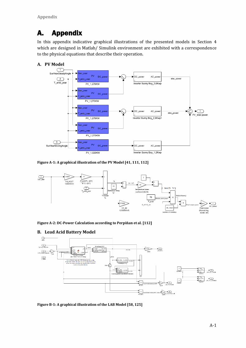
Appendix
A-1
A. Appendix In this appendix indicative graphical illustrations of the presented models in Section 4
which are designed in Matlab/ Simulink environment are exhibited with a correspondence
to the physical equations that describe their operation.
PV Model A.
Figure A-1: A graphical illustration of the PV Model [41, 111, 112]
Figure A-2: DC-Power Calculation according to Perpiñan et al. [112]
Lead Acid Battery Model B.
Figure B-1: A graphical illustration of the LAB Model [58, 125]
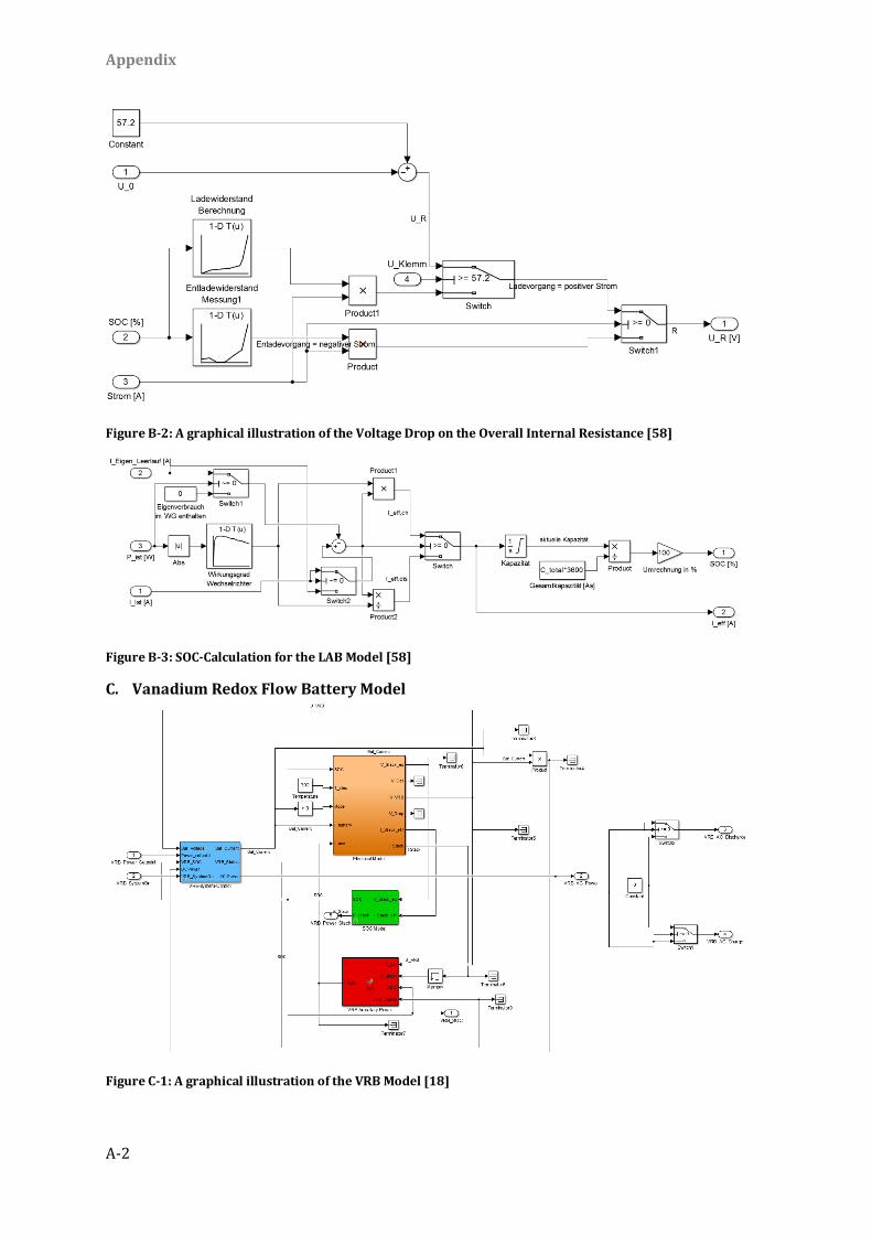
Appendix
A-2
Figure B-2: A graphical illustration of the Voltage Drop on the Overall Internal Resistance [58]
Figure B-3: SOC-Calculation for the LAB Model [58]
Vanadium Redox Flow Battery Model C.
Figure C-1: A graphical illustration of the VRB Model [18]
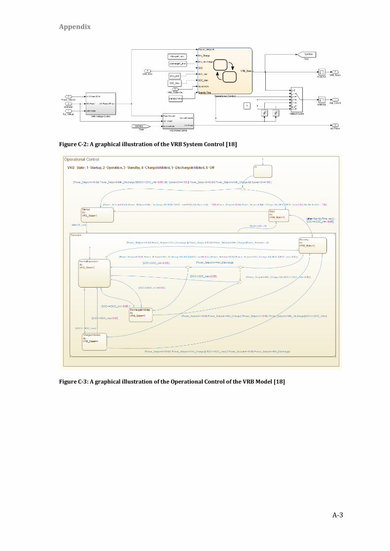
Appendix
A-3
Figure C-2: A graphical illustration of the VRB System Control [18]
Figure C-3: A graphical illustration of the Operational Control of the VRB Model [18]
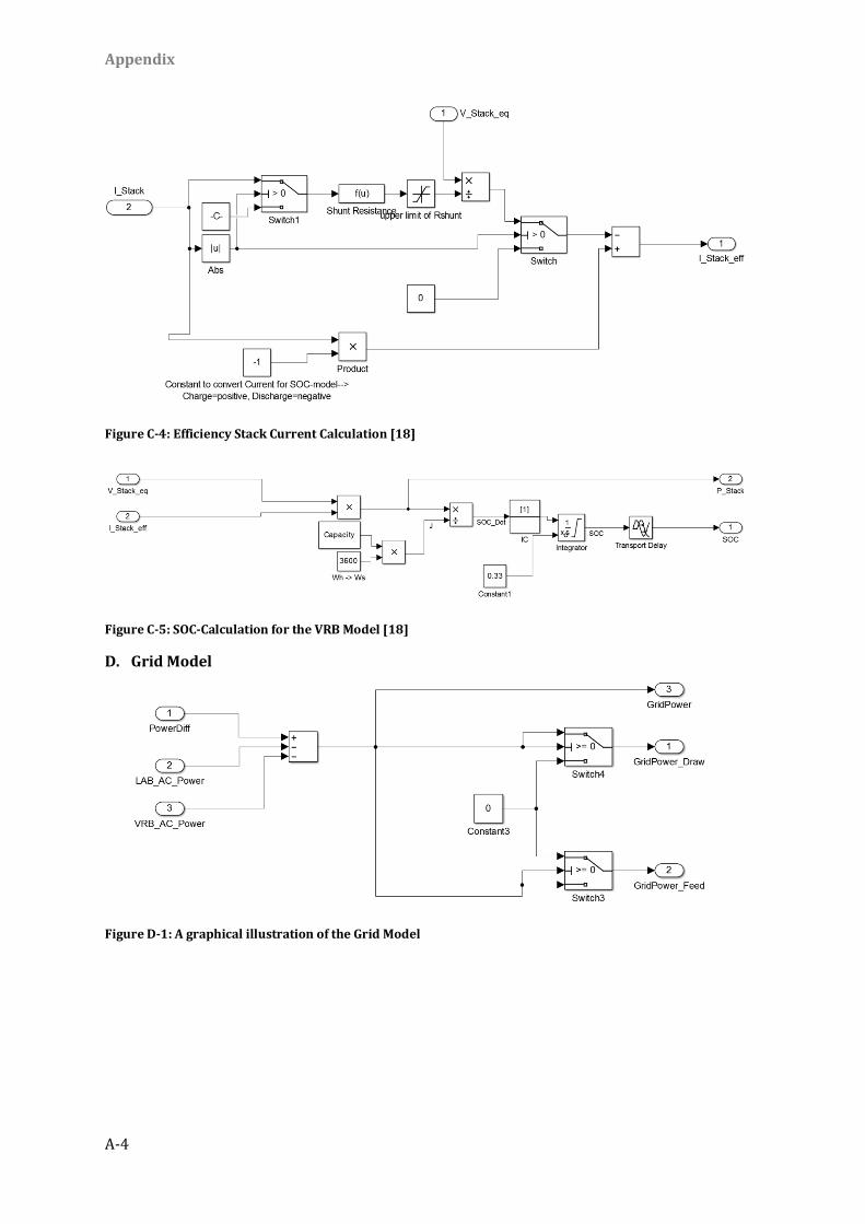
Appendix
A-4
Figure C-4: Efficiency Stack Current Calculation [18]
Figure C-5: SOC-Calculation for the VRB Model [18]
Grid Model D.
Figure D-1: A graphical illustration of the Grid Model