stage WECC Composite Load Modeling: A Double Deep Q ... WECC Composite Load Modeling.pdfDouble Deep Q-Learning Networks Approach A This work is funded by SGCC Science and Technology

> REPLACE THIS LINE WITH YOUR PAPER IDENTIFICATION NUMBER (DOUBLE-CLICK HERE TO EDIT) <

1

Abstract—With the increasing complexity of modern power

system, conventional dynamic load modeling with ZIP and

induction motors (ZIP + IM) is no longer adequate to address the

current load characteristic transitions. In recent years, the

Western Electricity Coordinating Council Composite Load Model

(WECC CLM) has shown to effectively capture the dynamic load

responses over traditional load models in various stability studies

and contingency analyses. However, a detailed WECC CLM

model typically has a high degree of complexity, with over one

hundred parameters, and no systematic approach to identifying

and calibrating these parameters. Enabled by the wide

deployment of PMUs and advanced deep learning algorithms,

proposed here is a double deep Q-learning network

(DDQN)-based, two-stage load modeling framework for the

WECC CLM. This two-stage method decomposes the complicated

WECC CLM for more efficient identification and does not

require explicit model details. In the stage one, the DDQN agent

determines a proper load composition that can approximate the

true transient dynamics. In the second stage, the remaining

parameters of the WECC CLM are selected with Monte-Carlo

simulations. The proposed method shows that the identified load

model is capable of accurately simulating the given dynamics of

the reference load model. In addition, the identified load model

has strong robustness to represent the reference load model under

a wide range of contingencies. The proposed framework is

verified using an IEEE 39-bus test system on commercial

simulation platforms.

Index Terms—Load modeling, deep reinforcement learning,

DDQN, load component identification, measurement-based.

I. INTRODUCTION

ccurate dynamic load modeling is critical for power

system transient stability analysis and various

simulation-based studies [1]-[2]. It is also known to improve

the power system operation flexibility, reduce system operating

costs, and better determine the corridor transfer limits [3]-[4].

In the past few decades, both industry and academic researchers

have widely used ZIP and induction motors (ZIP + IM) as the

composite load model (CLM) for quantifying load

characteristics [5]-[7], in which ZIP approximates the static

load transient behaviors and the IM approximates the dynamic

load transient behaviors. This ZIP + IM load model has shown

to be effective for simulating many dynamics in the power

system, but in recent years, industry has started to observe

various new load components, including single-phase IM,

distributed energy resources (DER), and loads interfaced via

power electronics that are being increasingly integrated into the

system. The high penetration of these new types of loads brings

profound changes to the transient characteristics at the load

end, which raises the necessity for more advanced load

modeling. For example, the well-known fault-induced,

delayed-voltage-recovery (FIDVR) event is caused by the

stalling of low-inertia single-phase IMs [8] when the fault

voltage is lower than their stall thresholds. An FIDVR event

poses potential voltage control losses and cascading failures in

the power system [9]; however, FIDVR cannot be modeled by a

conventional CLM model. Given these conditions, the Western

Electricity Coordinating Council Composite Load Model

(WECC CLM) is proposed.

To date, WECC CLM is available from multiple commercial

simulation tools such as the DSAToolsTM, GE PSLF, and

PowerWorld Simulator. However, the detailed model structure,

control logic, and parameter settings of the WECC CLM are

limited by most of the software vendors (PowerWorld

Simulator as a notable exception), and thus not transparent to

the public [10], which impacts WECC CLM’s general adoption

and practicality. Furthermore, lack of detailed open-source

information about the WECC CLM presents another major

roadblock for conducting load modeling and parameter

identification studies for system stability analysis.

Current WECC CLM works can be classified into two

groups, which are component-based methods that rely on load

surveys [11], [12] and measurement-based numerical fitting

methods [13], [14]. In [11] and [12], the WECC CLM’s

parameters are estimated from surveys of different customer

classes and load type statistics. However, the granularity and

accuracy of the survey data depend entirely on the survey

agency, and there are many assumptions being made that

cannot be definitively verified. In addition, the survey is

generally not up to date and does not reflect real-time

conditions. In practice, all these limitations bring challenges in

modeling the actual dynamic responses.

In another approach, authors in [13] and [14] numerically

solve the parameter-fitting problem using nonlinear least

squares estimators. In these methods, the parameter

identifiability assessment and dimension reduction are

conducted through sensitivity and dependency analysis.

Though sensitivity analysis reflects the impacts of the

individual parameter on the load dynamics, it fails to capture

the mutual dependency between two or more parameters, which

has been proved to be of great importance in composite load

Xinan Wang, Student Member, IEEE, Yishen Wang, Member, IEEE, Di Shi, Senior Member, IEEE，Jianhui Wang, Senior Member, IEEE, Zhiwei Wang, Senior Member, IEEE

Two-stage WECC Composite Load Modeling: A

Double Deep Q-Learning Networks Approach

A

This work is funded by SGCC Science and Technology Program under

contract no. SGSDYT00FCJS1700676. X. Wang, Y. Wang, D. Shi and Z. Wang are with GEIRI North America, San Jose, CA 95134, USA. X. Wang

and J. Wang are with the Department of Electrical and Computer Engineering,

Southern Methodist University, Dallas, TX 75205 USA.


2

dynamics [15], [16]. In [14], the authors define the parameter

dependency as the similarity of their influences on the dynamic

response trajectory. Such a dependency analysis still falls short

in factoring in the impact of multiple parameters on the load

transient dynamics at the same time. In fact, with over one

hundred parameters in the WECC CLM, the true interactions

among them are hard to fully assess.

This paper proposes a double deep Q-learning network

(DDQN)-based load modeling framework to conduct load

modeling on the WECC CLM. In this framework, the DDQN

agent serves as an optimization tool to estimate the key

parameters in WECC CLM. Similar deep reinforcement

learning-based optimization problems have also been discussed

in [17] and [18]. In [17], the authors apply the deep

deterministic policy gradient (DDPG) algorithm to determine

the values of five control setpoints in the cooling systems to

minimize the total data center cooling costs; in [18], the authors

use the deep Q-learning network (DQN) to identify the runtime

parameter in computer systems to improve the accuracy of the

cache expiration time estimation. For this proposed load

modeling work on WECC CLM, rather than directly

constructing states for all parameters, the first stage only builds

states for the load component fractions. These load component

fractions or states serve as the “abstracted features” to

characterize the full composite load models. The sequential

decision making [19] then relates to assess whether these states

can consistently represent the load model for future actions or

load fraction changes. The DRL agent thus learns the Q-values

for these states to obtain high rewards in the long run. In this

way, the identified load component fractions are relatively

robust to various conditions, which are another desirable

property for load modeling. The remaining parameters,

including the other top sensitive parameters as suggested in [14]

and [20], are identified in the second stage.

This method adopts the Transient Security Assessment Tools

(TSAT) from DSATools as the DDQN agent’s training

environment, which follows the state-of-art WECC model

validation progresses to comply with industry practitioners. As

such it is different from most nonlinear least square

estimator-based load modeling work. The method recasts the

load modeling for the WECC CLM into a two-stage learning

problem. In the first stage, a DDQN agent is trained to find a

load composition ratio that most likely represents the true

dynamic responses at the bus of interest. Then, in the second

stage, Monte-Carlo simulations are conducted to select the rest

of the load parameters for the load model. From the

Monte-Carlo simulations, the one set of parameters that best

approximates the true dynamic responses is chosen for the load

model. The specification [21] of the WECC CLM indicates that

each load component in the model represents the aggregation of

a specific type of load. Under such a composite load structure, it

has been observed in [22] and [23] that different load

composition ratios could have very similar transient dynamics.

Therefore, solving the load composition ratio first and

conducting the load parameter identification based on the

identified ratio can significantly reduce the problem’s

complexity and increase load parameter identification

computational efficiency. In addition, each parameter is

independently selected in stage two through Monte-Carlo

simulations, and the parameter identification criteria is to

evaluate the dynamic response reconstruction. This method

implicitly considers the dependency between two or more

parameters. Our proposed method offers the following unique

features and contributions:

1) A load modeling framework for the WECC CLM with

limited prior knowledge to model details. Only the

dynamic response curve is required to implement the

proposed learning framework.

2) The load model identified by this framework is robust to

various contingencies. The fitted load model is verified to

be effective to recover the true dynamics with different

fault locations, fault types and fault durations.

3) The proposed method is scalable to different composite

load structures: In the DDQN training environment, the

action taken by the agent is designed to be the load

fraction changes on different load types. This set up

allows the proposed method to be scaled from

conventional CLM load models such as ZIP + IM to

larger load models like the WECC CLM. The method can

be easily extended when WECC CLM is updated with

new load components, such as distributed energy

resources (DERs).

4) Applicable with limited data scenario: Unlike other

data-hungry supervised and unsupervised machine

learning methods, our DDQN approach only needs a few

sets of transient records to conduct load modeling, which

effectively overcome the data availability issue.

The remainder of this paper is organized as follows. Section

II discusses the load component definition in the WECC CLM

and the associated parameter selection range of each

component. Section III introduces the DDQN training

environment formulation and the customized reward function.

Section IV presents the case studies to validate the

effectiveness of the proposed method using the DSAToolsTM.

Section V provides concluding remarks and discussions on

future research.

II. WECC CLM INTRODUCTION

A. WECC CLM Structure

The WECC CLM is widely recognized as the state-of-the-art

load model [24] due its robustness in modeling a variety of load

compositions and its capability of simulating the electrical

distance between the end-users and the transmission

substations [9].

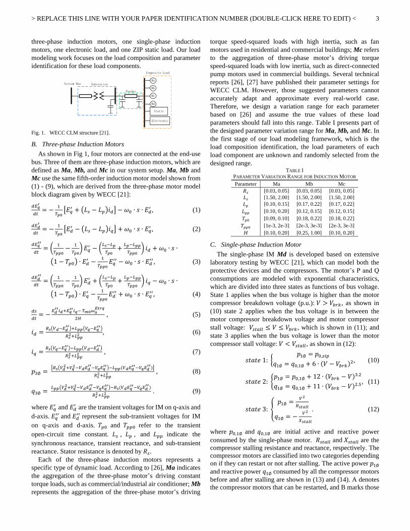
The detailed load structure for the WECC CLM is shown in

Fig. 1, which mainly consists of three parts: substation, feeder,

and load. The parameters for substation and feeder parts, such

as the substation shunt capacitance 𝐵𝑠𝑠 and transformer tap

settings [25] usually follow the industry convention and do not

have significant variance [23]-[27]. Therefore, in this paper, we

set the feeder and substation parameters following industrial

standard values [23]. The load in WECC CLM includes three


3

three-phase induction motors, one single-phase induction

motors, one electronic load, and one ZIP static load. Our load

modeling work focuses on the load composition and parameter

identification for these load components.

Ma

Mb

Mc

Md

Static

Electronic

System Bus Substation

Feeder

Composite Load

Fig. 1. WECC CLM structure [21].

B. Three-phase Induction Motors

As shown in Fig 1, four motors are connected at the end-use

bus. Three of them are three-phase induction motors, which are

defined as Ma, Mb, and Mc in our system setup. Ma, Mb and

Mc use the same fifth-order induction motor model shown from

(1) - (9), which are derived from the three-phase motor model

block diagram given by WECC [21]:

𝑑𝐸𝑞′

𝑑𝑡= −

1

𝑇𝑝0[𝐸𝑞

′ + (𝐿𝑠 − 𝐿𝑝)𝑖𝑑] − 𝜔0 ∙ 𝑠 ∙ 𝐸𝑑′ , (1)

𝑑𝐸𝑑′

𝑑𝑡= −

1

𝑇𝑝0[𝐸𝑑

′ − (𝐿𝑠 − 𝐿𝑝)𝑖𝑞] + 𝜔0 ∙ 𝑠 ∙ 𝐸𝑞′ , (2)

𝑑𝐸𝑞′′

𝑑𝑡= (

1

𝑇𝑝𝑝0−

1

𝑇𝑝0) 𝐸𝑞

′ − (𝐿𝑠−𝐿𝑝

𝑇𝑝0+

𝐿𝑝−𝐿𝑝𝑝

𝑇𝑝𝑝0) 𝑖𝑑 + 𝜔0 ∙ 𝑠 ∙

(1 − 𝑇𝑝0) ∙ 𝐸𝑑′ −

1

𝑇𝑝𝑝0𝐸𝑞′′ − 𝜔0 ∙ 𝑠 ∙ 𝐸𝑑

′′, (3)

𝑑𝐸𝑑′′

𝑑𝑡= (

1

𝑇𝑝𝑝0−

1

𝑇𝑝0) 𝐸𝑑

′ + (𝐿𝑠−𝐿𝑝

𝑇𝑝0+

𝐿𝑝−𝐿𝑝𝑝

𝑇𝑝𝑝0) 𝑖𝑞 − 𝜔0 ∙ 𝑠 ∙

(1 − 𝑇𝑝0) ∙ 𝐸𝑞′ −

1

𝑇𝑝𝑝0𝐸𝑑′′ + 𝜔0 ∙ 𝑠 ∙ 𝐸𝑞

′′, (4)

𝑑𝑠

𝑑𝑡= −

𝐸𝑑′′𝑖𝑑+𝐸𝑞

′′𝑖𝑞− 𝑇𝑚0𝜔0𝐸𝑡𝑟𝑞

2𝐻 , (5)

𝑖𝑑 =𝑅𝑠(𝑉𝑑−𝐸𝑑

′′)+𝐿𝑝𝑝(𝑉𝑞−𝐸𝑞′′)

𝑅𝑠2+𝐿𝑝𝑝

2 , (6)

𝑖𝑞 =𝑅𝑠(𝑉𝑞−𝐸𝑞

′′)−𝐿𝑝𝑝(𝑉𝑑−𝐸𝑑′′)


2 , (7)

𝑝3∅ = [𝑅𝑠(𝑉𝑑

2+𝑉𝑞2−𝑉𝑑𝐸𝑑

′′−𝑉𝑞𝐸𝑞′′)−𝐿𝑝𝑝(𝑉𝑑𝐸𝑞

′′−𝑉𝑞𝐸𝑑′′)]


2 , (8)

𝑞3∅ = 𝐿𝑝𝑝(𝑉𝑑

2+𝑉𝑞2−𝑉𝑑𝐸𝑑

′′−𝑉𝑞𝐸𝑞′′)−𝑅𝑠(𝑉𝑑𝐸𝑞

′′−𝑉𝑞𝐸𝑑′′)


2 . (9)

where 𝐸𝑞′ and 𝐸𝑑

′ are the transient voltages for IM on q-axis and

d-axis. 𝐸𝑞′′ and 𝐸𝑑

′′ represent the sub-transient voltages for IM

on q-axis and d-axis. 𝑇𝑝0 and 𝑇𝑝𝑝0 refer to the transient

open-circuit time constant. 𝐿𝑠 , 𝐿𝑝 , and 𝐿𝑝𝑝 indicate the

synchronous reactance, transient reactance, and sub-transient

reactance. Stator resistance is denoted by 𝑅𝑠. Each of the three-phase induction motors represents a

specific type of dynamic load. According to [26], Ma indicates

the aggregation of the three-phase motor’s driving constant

torque loads, such as commercial/industrial air conditioner; Mb

represents the aggregation of the three-phase motor’s driving

torque speed-squared loads with high inertia, such as fan

motors used in residential and commercial buildings; Mc refers

to the aggregation of three-phase motor’s driving torque

speed-squared loads with low inertia, such as direct-connected

pump motors used in commercial buildings. Several technical

reports [26], [27] have published their parameter settings for

WECC CLM. However, those suggested parameters cannot

accurately adapt and approximate every real-world case.

Therefore, we design a variation range for each parameter

based on [26] and assume the true values of these load

parameters should fall into this range. Table I presents part of

the designed parameter variation range for Ma, Mb, and Mc. In

the first stage of our load modeling framework, which is the

load composition identification, the load parameters of each

load component are unknown and randomly selected from the

designed range. TABLE I

PARAMETER VARIATION RANGE FOR INDUCTION MOTOR Parameter Ma Mb Mc

𝑅𝑠 [0.03, 0.05] [0.03, 0.05] [0.03, 0.05]

𝐿𝑠 [1.50, 2.00] [1.50, 2.00] [1.50, 2.00]

𝐿𝑝 [0.10, 0.15] [0.17, 0.22] [0.17, 0.22]

𝐿𝑝𝑝 [0.10, 0.20] [0.12, 0.15] [0.12, 0.15]

𝑇𝑝0 [0.09, 0.10] [0.18, 0.22] [0.18, 0.22]

𝑇𝑝𝑝0 [1e-3, 2e-3] [2e-3, 3e-3] [2e-3, 3e-3]

H [0.10, 0.20] [0.25, 1.00] [0.10, 0.20]

C. Single-phase Induction Motor

The single-phase IM Md is developed based on extensive

laboratory testing by WECC [21], which can model both the

protective devices and the compressors. The motor’s P and Q

consumptions are modeled with exponential characteristics,

which are divided into three states as functions of bus voltage.

State 1 applies when the bus voltage is higher than the motor

compressor breakdown voltage (p.u.): 𝑉 > 𝑉𝑏𝑟𝑘, as shown in

(10) state 2 applies when the bus voltage is in between the

motor compressor breakdown voltage and motor compressor

stall voltage: 𝑉𝑠𝑡𝑎𝑙𝑙 ≤ 𝑉 ≤ 𝑉𝑏𝑟𝑘, which is shown in (11); and

state 3 applies when the bus voltage is lower than the motor

compressor stall voltage: 𝑉 < 𝑉𝑠𝑡𝑎𝑙𝑙 , as shown in (12):

𝑠𝑡𝑎𝑡𝑒 1: {𝑝1∅ = 𝑝0,𝑧𝑖𝑝

𝑞1∅ = 𝑞0,1∅ + 6 ∙ (𝑉 − 𝑉𝑏𝑟𝑘)2, (10)

𝑠𝑡𝑎𝑡𝑒 2: {𝑝1∅ = 𝑝0,1∅ + 12 ∙ (𝑉𝑏𝑟𝑘 − 𝑉)

3.2

𝑞1∅ = 𝑞0,1∅ + 11 ∙ (𝑉𝑏𝑟𝑘 − 𝑉)2.5, (11)

𝑠𝑡𝑎𝑡𝑒 3: {𝑝1∅ =

𝑉2

𝑅𝑠𝑡𝑎𝑙𝑙

𝑞1∅ = −𝑉2

𝑋𝑠𝑡𝑎𝑙𝑙

. (12)

where 𝑝0,1∅ and 𝑞0,1∅ are initial active and reactive power

consumed by the single-phase motor. 𝑅𝑠𝑡𝑎𝑙𝑙 and 𝑋𝑠𝑡𝑎𝑙𝑙 are the

compressor stalling resistance and reactance, respectively. The

compressor motors are classified into two categories depending

on if they can restart or not after stalling. The active power 𝑝1∅

and reactive power 𝑞1∅ consumed by all the compressor motors

before and after stalling are shown in (13) and (14). A denotes

the compressor motors that can be restarted, and B marks those


4

that cannot be restarted. In (13), 𝐹𝑟𝑠𝑡 refers to the ratio between

motor loads that can restart and the total motor loads. In (14),

𝑉𝑟𝑠𝑡 refers to the restarting voltage threshold for the stalled

motors. 𝑓(𝑉 > 𝑉𝑟𝑠𝑡) is the function of the P, Q recovery rate of

the compressor motors that can be restarted.

𝑏𝑒𝑓𝑜𝑟𝑒 𝑠𝑡𝑎𝑙𝑙𝑖𝑛𝑔: {𝑝𝐴 = 𝑝1∅ ∗ 𝐹𝑟𝑠𝑡𝑞𝐴 = 𝑞1∅ ∗ 𝐹𝑟𝑠𝑡

, , (13)

𝑎𝑓𝑡𝑒𝑟 𝑠𝑡𝑎𝑙𝑙𝑖𝑛𝑔: {𝑝1∅ = 𝑝𝐴 ∙ 𝑓(𝑉 > 𝑉𝑟𝑠𝑡) + 𝑝𝐵,𝑠𝑡𝑎𝑙𝑙𝑞1∅ = 𝑞𝐴 ∙ 𝑓(𝑉 > 𝑉𝑟𝑠𝑡) + 𝑞𝐵,𝑠𝑡𝑎𝑙𝑙

. (14)

Other than the voltage stalling feature introduced here, WECC

CLM also incorporates a thermal relay feature into the

single-phase motor, and the detailed information can be found

in [21]. Md’s compressor dynamic model is the same as the

three-phase IM as Ma, Mb, and Mc. We design the parameter

selection range for Md according to [26]. The values of some

critical parameters such as 𝑉𝑠𝑡𝑎𝑙𝑙 , 𝑉𝑟𝑠𝑡 , 𝑉𝑏𝑟𝑘, and 𝐹𝑟𝑠𝑡 are

selected from the ranges shown in Table II. TABLE II

PARAMETER VARIATION RANGE FOR SINGLE-PHASE IM Parameter 𝑉𝑏𝑟𝑘 𝑉𝑟𝑠𝑡 𝑉𝑠𝑡𝑎𝑙𝑙 𝐹𝑟𝑠𝑡

[0.85, 0.90] [0.92, 0.96] [0.55, 0.65] [0.15, 0.30]

D. Static Load Model: ZIP

The standard ZIP model is used in WECC CLM to represent

the static load. The corresponding active and reactive power are

written in (15)-(17):

𝑝𝑧𝑖𝑝 = 𝑝0,𝑧𝑖𝑝 ∙ (𝑝1𝑐 ∙ (𝑉

𝑉𝑜)2

+ 𝑝2𝑐 ∙𝑉

𝑉𝑜+ 𝑝3𝑐), (15)

𝑞𝑧𝑖𝑝 = 𝑞0,𝑧𝑖𝑝 ∙ (𝑞1𝑐 ∙ (𝑉

𝑉𝑜)2

+ 𝑞2𝑐 ∙𝑉

𝑉𝑜+ 𝑞3𝑐), (16)

{𝑝1𝑐 + 𝑝2𝑐 + 𝑝3𝑐 = 1, (0 ≤ 𝑝1𝑐 , 𝑝2𝑐 , 𝑝3𝑐 ≤ 1)𝑞1𝑐 + 𝑞2𝑐 + 𝑞3𝑐 = 1, (0 ≤ 𝑞1𝑐 , 𝑞2𝑐 , 𝑞3𝑐 ≤ 1)

. (17)

where, 𝑝0,𝑧𝑖𝑝 and 𝑞0,𝑧𝑖𝑝 are the initial active and reactive

power consumed by the ZIP load. 𝑝1𝑐 , 𝑝2𝑐 , and 𝑝3𝑐 are the

coefficients for the active power of constant impedance,

constant current, and constant power load. 𝑞1𝑐 , 𝑞2𝑐, and 𝑞3𝑐 are

the coefficients for reactive power of constant impedance,

constant current, and constant power load. To model the

diversity of ZIP load, the 𝑝1𝑐,2𝑐,3𝑐 and 𝑞1𝑐,2𝑐,3𝑐 are set to be

random within the boundary shown in (17).

E. Electronic Load

The electronic load model in the WECC CLM aims to

simulate the linear load tripping phenomenon of electronics. It

is modeled as a conditional linear function of the bus voltage V,

as shown from the (18)-(19). 𝑉𝑑1 represents the voltage

threshold at which the electronic load starts to trip, 𝑉𝑑2

indicates the voltage threshold at which all the electronic load

trips, 𝑉𝑚𝑖𝑛 tracks the minimum bus voltage during the transient,

𝑓𝑟𝑐𝑒𝑙 indicates the fraction of electronic load that can be

restarted after a fault is cleared. In (20), 𝑝𝑓𝑒𝑙𝑐 denotes the power

factor of electronic load (default as 1), and 𝑝0,𝑒𝑙𝑐 refers to the

initial power of electronic load. The parameter variation ranges

for electronic load are the shown in Table III.

𝑓𝑣𝑙 =

{

1𝑉−𝑉𝑑2

𝑉𝑑1−𝑉𝑑2𝑉𝑚𝑖𝑛−𝑉𝑑2+𝑓𝑟𝑐𝑒𝑙∙(𝑉−𝑉𝑚𝑖𝑛)

𝑉𝑑1−𝑉𝑑2

0

, (18)

𝑝𝑒𝑙𝑐 = 𝑓𝑣𝑙 ∙ 𝑝0,𝑒𝑙𝑐 , (19)

𝑞𝑒𝑙𝑐 = tan (cos−1(𝑝𝑓𝑒𝑙𝑐)) ∗ 𝑝𝑒𝑙𝑐 . (20)

TABLE III PARAMETER VARIATION RANGE FOR ELECTRONIC LOAD

Parameter 𝑉𝑑1 𝑉𝑑2 𝑝𝑓𝑒𝑙𝑐

[0.60, 0.70] [0.50, 0.55] 1

F. Identify the Composition of the Composite Load

In a composite load model, different load composition can

induce very similar dynamic responses [22], [23]. It has been

observed in [22] that a different load composition of a big IM

and a small IM could have very similar load dynamic

responses. This multi-solution phenomenon on load

composition is even more common in the WECC CLM due to

the multiple IMs in place. Our proposed two-stage load

modeling method can effectively find near-optimal load

compositions in stage one; and then in stage two, the other load

parameters can be efficiently identified. To demonstrate the

importance of identifying the load composition before fitting

other parameters, we conduct a fitting loss comparison.

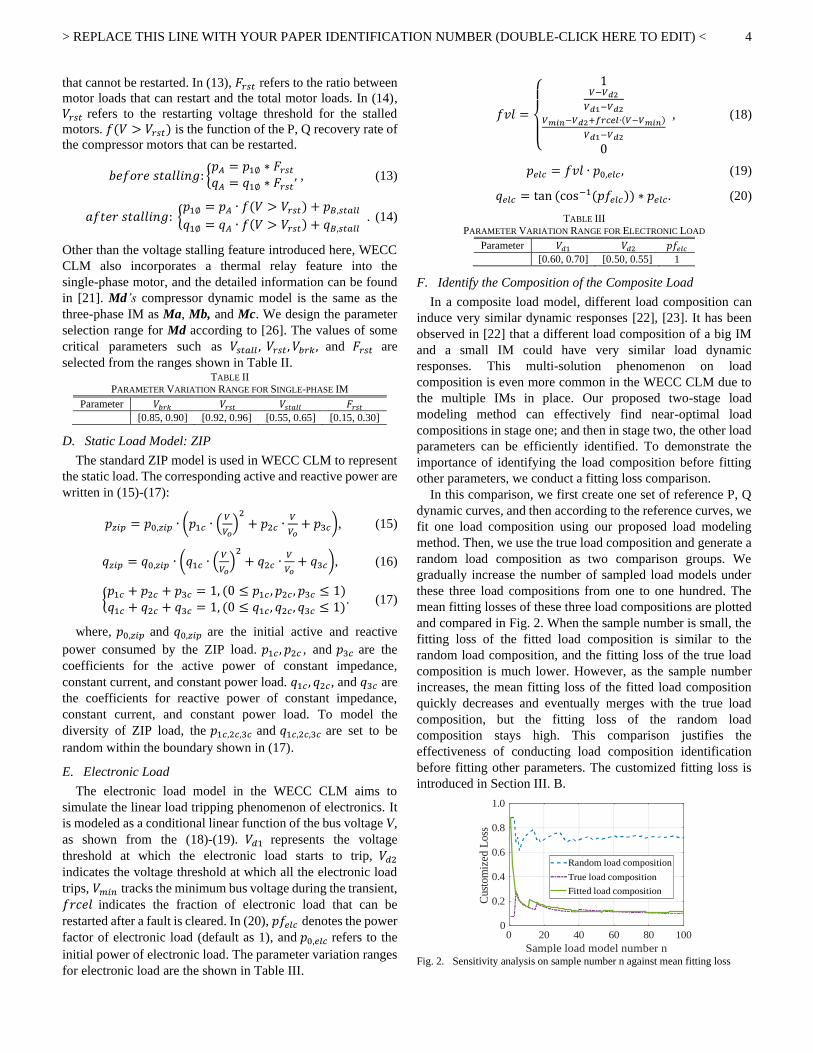
In this comparison, we first create one set of reference P, Q

dynamic curves, and then according to the reference curves, we

fit one load composition using our proposed load modeling

method. Then, we use the true load composition and generate a

random load composition as two comparison groups. We

gradually increase the number of sampled load models under

these three load compositions from one to one hundred. The

mean fitting losses of these three load compositions are plotted

and compared in Fig. 2. When the sample number is small, the

fitting loss of the fitted load composition is similar to the

random load composition, and the fitting loss of the true load

composition is much lower. However, as the sample number

increases, the mean fitting loss of the fitted load composition

quickly decreases and eventually merges with the true load

composition, but the fitting loss of the random load

composition stays high. This comparison justifies the

effectiveness of conducting load composition identification

before fitting other parameters. The customized fitting loss is

introduced in Section III. B.

Fig. 2. Sensitivity analysis on sample number n against mean fitting loss

0 20 40 60 80 100

Sample load model number n

0

0.2

0.4

0.6

0.8

1.0

Cust

om

ized

Loss

Random load composition

True load composition

Fitted load composition


5

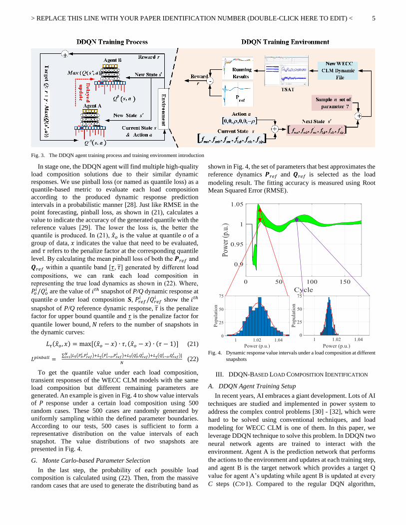
Fig. 3. The DDQN agent training process and training environment introduction

In stage one, the DDQN agent will find multiple high-quality

load composition solutions due to their similar dynamic

responses. We use pinball loss (or named as quantile loss) as a

quantile-based metric to evaluate each load composition

according to the produced dynamic response prediction

intervals in a probabilistic manner [28]. Just like RMSE in the

point forecasting, pinball loss, as shown in (21), calculates a

value to indicate the accuracy of the generated quantile with the

reference values [29]. The lower the loss is, the better the

quantile is produced. In (21), �̂�𝜊 is the value at quantile 𝜊 of a

group of data, 𝑥 indicates the value that need to be evaluated,

and 𝜏 refers to the penalize factor at the corresponding quantile

level. By calculating the mean pinball loss of both the 𝑷𝑟𝑒𝑓 and

𝑸𝑟𝑒𝑓 within a quantile band [𝜏, 𝜏] generated by different load

compositions, we can rank each load composition in

representing the true load dynamics as shown in (22). Where,

𝑃𝜊𝑖/𝑄𝜊

𝑖 are the value of 𝑖𝑡ℎ snapshot of P/Q dynamic response at

quantile 𝜊 under load composition S, 𝑃𝑟𝑒𝑓𝑖 /𝑄𝑟𝑒𝑓

𝑖 show the 𝑖𝑡ℎ

snapshot of P/Q reference dynamic response, 𝜏 is the penalize

factor for upper bound quantile and 𝜏 is the penalize factor for

quantile lower bound, 𝑁 refers to the number of snapshots in

the dynamic curves:

𝐿𝜏(�̂�𝜊, 𝑥) = max[(�̂�𝜊 − 𝑥) ∙ 𝜏, (�̂�𝜊 − 𝑥) ∙ (𝜏 − 1)] (21)

𝐿𝑝𝑖𝑛𝑏𝑎𝑙𝑙 = ∑ [𝐿𝜏(𝑃𝜊

𝑖 ,𝑃𝑟𝑒𝑓𝑖 )+𝐿𝜏(𝑃1−𝜊

𝑖 ,𝑃𝑟𝑒𝑓𝑖 )+𝐿𝜏(𝑄𝜊

𝑖 ,𝑄𝑟𝑒𝑓𝑖 )+𝐿𝜏(𝑄1−𝜊

𝑖 ,𝑄𝑟𝑒𝑓𝑖 )]𝑁

𝑖=1

𝑁 (22)

To get the quantile value under each load composition,

transient responses of the WECC CLM models with the same

load composition but different remaining parameters are

generated. An example is given in Fig. 4 to show value intervals

of 𝑃 response under a certain load composition using 500

random cases. These 500 cases are randomly generated by

uniformly sampling within the defined parameter boundaries.

According to our tests, 500 cases is sufficient to form a

representative distribution on the value intervals of each

snapshot. The value distributions of two snapshots are

presented in Fig. 4.

G. Monte Carlo-based Parameter Selection

In the last step, the probability of each possible load

composition is calculated using (22). Then, from the massive

random cases that are used to generate the distributing band as

shown in Fig. 4, the set of parameters that best approximates the

reference dynamics 𝑷𝑟𝑒𝑓 and 𝑸𝑟𝑒𝑓 is selected as the load

modeling result. The fitting accuracy is measured using Root

Mean Squared Error (RMSE).

Fig. 4. Dynamic response value intervals under a load composition at different

snapshots

III. DDQN-BASED LOAD COMPOSITION IDENTIFICATION

A. DDQN Agent Training Setup

In recent years, AI embraces a giant development. Lots of AI

techniques are studied and implemented in power system to

address the complex control problems [30] - [32], which were

hard to be solved using conventional techniques, and load

modeling for WECC CLM is one of them. In this paper, we

leverage DDQN technique to solve this problem. In DDQN two

neural network agents are trained to interact with the

environment. Agent A is the prediction network that performs

the actions to the environment and updates at each training step,

and agent B is the target network which provides a target Q

value for agent A’s updating while agent B is updated at every

C steps (C≫1). Compared to the regular DQN algorithm,


6

DDQN has better training stability as it avoids the positive bias

propagation caused by the max function in a Bellman equation

[33]. At each state, the environment responds to the taken

action. This response is interpreted as reward or penalty. Both

agent A and agent B learn the action-reward function 𝑄(𝑠, 𝑎) by iteratively updating the Q value following (23), which is

fundamentally a Bellman equation. In (23), the 𝑄𝐴(𝑠, 𝑎) and

𝑄𝐵(𝑠, 𝑎) denote the Q functions learned by agent A and agent

B; 𝑠 is the current state; 𝑎 refers to the current action taken by

the agent. 𝛿 represents the learning rate, which determines to

which extent the newly acquired information overrides the old

information. 𝛾 indicates the discount factor, which essentially

determines how much the reinforcement learning agent weights

rewards in the long-term future relative to those in the

immediate future. 𝑟 is the immediate reward/penalty by taking

action 𝑎 at state 𝑠; 𝑠′ is the new state transient from 𝑠 after

action 𝑎 is taken.

𝑄𝐴(𝑠, 𝑎) = (1 − 𝛼)𝑄𝐴(𝑠, 𝑎) + 𝛿 ⋅ (𝑟 + 𝛾 ⋅

max𝑄𝐵(𝑠′, 𝑎)) (23)

Function 𝑄𝐴(𝑠, 𝑎) updates at every step following (23), but

function 𝑄𝐵(𝑠, 𝑎) updates every C steps (C≫1). In such a way,

the temporal difference (TD) error is created, which serves as

the optimization target for the agent, as shown in (24).

min (ℒ) = ‖𝑄𝐴(𝑠, 𝑎) − 𝑟 − 𝛾 ⋅ max𝑄𝐵(𝑠′, 𝑎)‖ (24)

In this application, the state is defined as the load composition

fraction of each load component: 𝑠 =[𝑓𝑚𝑎 , 𝑓𝑚𝑏 , 𝑓𝑚𝑐 , 𝑓1∅, 𝑓𝑒𝑙𝑐 , 𝑓𝑧𝑖𝑝]. The summation of 𝑠 is always one

to represent the full load. The actions to be taken by the agents

are the pair-wise load fraction modification: 𝑎 =[⋯ , 𝜌,⋯ ,−𝜌,⋯ ]. 𝜌 is the fraction modification value, which

is designed as 0.01 in the case study. Each 𝑎𝑡 only has two

non-zero elements, which are 𝜌 and −𝜌 . In this case, the

summation of 𝑠 is guaranteed to remain one at each step. For

WECC CLM in the study, there are six load components.

Considering the fraction has plus/minus two directions to

update, the total number of two-combinations from six

elements is 𝐴62 = 6 × 5 = 30. The training environment is the

IEEE 39-bus system built in the Transient Security Assessment

Tool (TSAT) in DSAToolsTM. Fig. 3 shows the DDQN training

process and the training environment. Observed from the

training environment, when a new state 𝑠′ is reached, n sets of

parameters θ will be sampled, which are then combined with 𝑠′ to form n dynamic files. The n dynamic files are run in the

TSAT in order to calculate the reward. In our work, n is

selected as 20 to efficiently identify the good load composition

candidates through the sensitivity analysis shown in Fig. 2.

Algorithm I: DDQN Training for WECC CLM

Input: Reference dynamic responses 𝑃𝑟𝑒𝑓 and 𝑄𝑟𝑒𝑓.

Output: Load composition and load parameters

Initialize 𝜆, 𝛾, ε, η，NN. A, NN. B and memory buffer M

For i in range (number of episode)

s←reset.enviroment(); ε← ε∙ η; r_sum←0; tik←0; NN. B←NN. A;

While tik ≤ 80:

If rand(1) < ε:

a← 𝒂(randi(|30|))

Else:

a← 𝒂(argmax(NN. A. predict(s)))

End

𝒔′,r←execute.TSAT(s, a)

If r>λ

Terminate Episode i.

Else

Step1: 𝑸𝑩(𝒔, 𝑎) = NN.B. predict(𝒔, 𝑎) Step2: 𝑸𝑨(𝒔) = NN.A. predict(𝒔) Step3: 𝑸𝑨(𝒔)(index(𝑎 in 𝒂)) = 𝑸𝑩(𝒔, 𝑎) + 𝑟

Sample a batch of transitions D from M

Repeat the Step 1 to Step 3 for each sample in D.

NN. A. fit([s, 𝒔𝑫],[𝑸𝑨(𝒔),𝑸𝑫]) M←[𝒔, a, 𝒔′, r]

s ← 𝒔′ r_sum= r_sum+r

End

r_list.append(r_sum)

End

The pseudo-code for the DDQN agent training is shown in

Algorithm I. In the training process the epsilon-greedy

searching policy and the memory replay buffer are applied, and

the detailed introduction to them can be found from [34], [35],

which will not be discussed in this paper. In our application, the

memory buffer size is designed as 2,000.

B. Customized Reward Function

The reward in our application is a negative value that

represents the transient P and Q curve fitting losses. The

training goal is to maximize the reward in (25) or equivalently

minimize the fitting losses. A higher reward means a higher

fitting accuracy. At each new state, the dynamic responses are

compared with the reference responses to get a reward r, which

will be further interpreted into a Q value to update the agent A

and agent B. However, the classic RMSE loss function cannot

properly differentiate the desirable load compositions from the

undesirable ones. This phenomenon is further explained later.

Therefore, a customized loss function is developed to better

capture the dynamic features of the transient curves as shown in

(25) and (26):

𝑟 = −𝛼 ∙ 𝑟𝑅𝑀𝑆𝐸 − 𝛽 ∙ 𝑟𝑡𝑟𝑒𝑛𝑑 − 𝑟𝑠𝑡𝑒𝑝. (25)

𝑟𝑡𝑟𝑒𝑛𝑑 =∑ |𝑖𝑑𝑥𝑚𝑖𝑛

𝑖 −𝑖𝑑𝑥𝑚𝑖𝑛𝑟𝑒𝑓

|+|𝑖𝑑𝑥𝑚𝑎𝑥𝑖 −𝑖𝑑𝑥𝑚𝑎𝑥

𝑟𝑒𝑓|𝑛

𝑖=1

𝐾 (26)

where 𝑟𝑅𝑀𝑆𝐸 denotes the RMSE between 𝑷𝑡𝑒𝑠𝑡 , 𝑸𝑡𝑒𝑠𝑡 and

𝑷𝑟𝑒𝑓 , 𝑸𝑟𝑒𝑓 . In equation (25), the regularization term 𝑟𝑡𝑟𝑒𝑛𝑑

represents the time index mismatch of peak and valley values

between 𝑷𝑡𝑒𝑠𝑡 , 𝑸𝑡𝑒𝑠𝑡 and 𝑷𝑟𝑒𝑓 , 𝑸𝑟𝑒𝑓 . 𝛼 and 𝛽 are the weights

of term 𝑟𝑅𝑀𝑆𝐸 and 𝑟𝑡𝑟𝑒𝑛𝑑. In equation (26), K is a constant that

scales down the index mismatch between 𝑷𝑡𝑒𝑠𝑡 , 𝑸𝑡𝑒𝑠𝑡 curves

and the 𝑷𝑟𝑒𝑓 , 𝑸𝑟𝑒𝑓 , 𝑖𝑑𝑥𝑚𝑖𝑛/𝑚𝑎𝑥𝑖 refers to the index of the

minimum/maximum value in the ith 𝑷𝑡𝑒𝑠𝑡 , 𝑸𝑡𝑒𝑠𝑡 , and

𝑖𝑑𝑥𝑚𝑖𝑛/𝑚𝑎𝑥𝑟𝑒𝑓

indicates the index of the minimum/maximum

value of 𝑷𝑟𝑒𝑓 , 𝑸𝑟𝑒𝑓 . The values of α, β, and K are tuned so that

the value of −𝛼 ∙ 𝑟𝑅𝑀𝑆𝐸 − 𝛽 ∙ 𝑟𝑡𝑟𝑒𝑛𝑑 − 𝑟𝑠𝑡𝑒𝑝 is normalized into

the range of [-1, 0]. This term explicitly differentiates the

desirable fitting results from others and enforces the similar

peak and valley timestamps as 𝑷𝑟𝑒𝑓 , 𝑸𝑟𝑒𝑓 . Another


7

regularization term 𝑟𝑠𝑡𝑒𝑝 is a constant penalty for each step of

searching, which facilitates the agent’s training speed. Such

loss function is fundamentally a similarity-based measure, and

this type of metrics is commonly used in load modeling

techniques [36]. By using this customized loss function, a

generic fitting accuracy threshold λ can then be set as the

episode termination condition. We show some example plots in

Fig. 5 to better explain the effects of this customized loss

function.

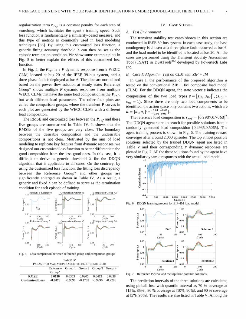
In Fig. 5, the 𝑷𝑟𝑒𝑓 is a P dynamic response from a WECC

CLM, located at bus 20 of the IEEE 39-bus system, and a

three-phase fault is deployed at bus 6. The plots are normalized

based on the power flow solution at steady state; Reference

Group* shows multiple P dynamic responses from multiple

WECC CLMs that have the same load composition as the 𝑷𝑟𝑒𝑓 ,

but with different load parameters. The other four plots are

called the comparison groups, where the transient P curves in

each plot are generated by the WECC CLMs with a different

load composition.

The RMSE and customized loss between the 𝑷𝑟𝑒𝑓 and these

five groups are summarized in Table IV. It shows that the

RMSEs of the five groups are very close. The boundary

between the desirable composition and the undesirable

compositions is not clear. Motivated by the aim of load

modeling to replicate key features from dynamic responses, we

designed our customized loss function to better differentiate the

good composition from the less good ones. In this case, it is

difficult to derive a generic threshold λ for the DDQN

algorithm that is applicable to all cases. On the contrary, by

using the customized loss function, the fitting loss discrepancy

between the Reference Group* and other groups are

significantly enlarged as shown in Table IV. As a result, a

generic and fixed λ can be defined to serve as the termination

condition for each episode of training.

Fig. 5. Loss comparison between reference group and comparison groups

TABLE IV PARAMETER VARIATION RANGE FOR ELECTRONIC LOAD Reference

Group*

Group 1 Group 2 Group 3 Group 4

RMSE 0.0136 0.0353 0.0205 0.0413 0.0338

Customized Loss -0.0078 -0.9596 -0.1702 -0.9996 -0.7206

IV. CASE STUDIES

A. Test Environment

The transient stability test cases shown in this section are

conducted in IEEE 39-bus system. In each case study, the base

contingency is chosen as a three-phase fault occurred at bus 6,

and the load model to be identified is located at bus 20. All the

cases are performed using the Transient Security Assessment

Tool (TSAT) in DSAToolsTM developed by Powertech Labs

Inc.

B. Case I: Algorithm Test on CLM with ZIP + IM

In Case I, the performance of the proposed algorithm is

tested on the conventional ZIP + IM composite load model

(CLM). For the DDQN agent, the state vector s indicates the

composition of the two load types 𝒔 = [𝑠𝑧𝑖𝑝, 𝑠𝐼𝑀]𝑇, (𝑠𝑧𝑖𝑝 +

𝑠𝐼𝑀 = 1) . Since there are only two load components to be

identified, the action space only contains two actions, which are

𝒂 = [𝑎1, 𝑎2]𝑇=[ 0.01

−0.01−0.010.01

].

The reference load composition is 𝒔𝑟𝑒𝑓 = [0.2937,0.7063]𝑇.

The DDQN agent starts to search for possible solutions from a

randomly generated load composition [0.4935,0.5065]. The

agent training process is shown in Fig. 6. The training reward

converges after around 2,000 episodes. The top 3 most possible

solutions selected by the trained DDQN agent are listed in

Table V and their corresponding P dynamic responses are

plotted in Fig. 7. All the three solutions found by the agent have

very similar dynamic responses with the actual load model.

Fig. 6. DDQN learning process for ZIP+IM load model

Fig. 7. Reference P curve and the top three possible solutions

The prediction intervals of the three solutions are calculated

using pinball loss with quantile interval as 70 % coverage at

[15%, 85%], 80 % coverage at [10%, 90%], and 90 % coverage

at [5%, 95%]. The results are also listed in Table V. Among the


8

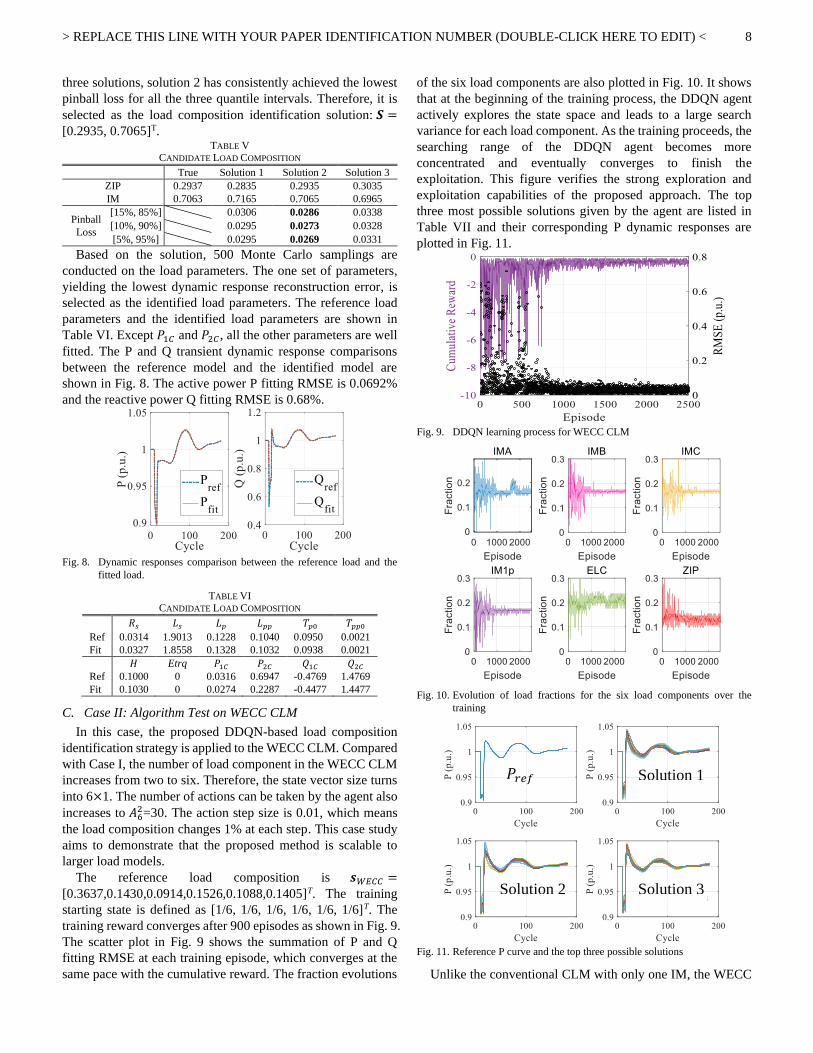
three solutions, solution 2 has consistently achieved the lowest

pinball loss for all the three quantile intervals. Therefore, it is

selected as the load composition identification solution: 𝑺 =

[0.2935, 0.7065]T. TABLE V

CANDIDATE LOAD COMPOSITION True Solution 1 Solution 2 Solution 3

ZIP 0.2937 0.2835 0.2935 0.3035

IM 0.7063 0.7165 0.7065 0.6965

Pinball

Loss

[15%, 85%] 0.0306 0.0286 0.0338

[10%, 90%] 0.0295 0.0273 0.0328

[5%, 95%] 0.0295 0.0269 0.0331

Based on the solution, 500 Monte Carlo samplings are

conducted on the load parameters. The one set of parameters,

yielding the lowest dynamic response reconstruction error, is

selected as the identified load parameters. The reference load

parameters and the identified load parameters are shown in

Table VI. Except 𝑃1𝐶 and 𝑃2𝐶 , all the other parameters are well

fitted. The P and Q transient dynamic response comparisons

between the reference model and the identified model are

shown in Fig. 8. The active power P fitting RMSE is 0.0692%

and the reactive power Q fitting RMSE is 0.68%.

Fig. 8. Dynamic responses comparison between the reference load and the

fitted load.

TABLE VI CANDIDATE LOAD COMPOSITION

𝑅𝑠 𝐿𝑠 𝐿𝑝 𝐿𝑝𝑝 𝑇𝑝0 𝑇𝑝𝑝0

Ref 0.0314 1.9013 0.1228 0.1040 0.0950 0.0021

Fit 0.0327 1.8558 0.1328 0.1032 0.0938 0.0021

𝐻 Etrq 𝑃1𝐶 𝑃2𝐶 𝑄1𝐶 𝑄2𝐶

Ref 0.1000 0 0.0316 0.6947 -0.4769 1.4769

Fit 0.1030 0 0.0274 0.2287 -0.4477 1.4477

C. Case II: Algorithm Test on WECC CLM

In this case, the proposed DDQN-based load composition

identification strategy is applied to the WECC CLM. Compared

with Case I, the number of load component in the WECC CLM

increases from two to six. Therefore, the state vector size turns

into 6×1. The number of actions can be taken by the agent also

increases to 𝐴62=30. The action step size is 0.01, which means

the load composition changes 1% at each step. This case study

aims to demonstrate that the proposed method is scalable to

larger load models.

The reference load composition is 𝒔𝑊𝐸𝐶𝐶 =

[0.3637,0.1430,0.0914,0.1526,0.1088,0.1405]T. The training

starting state is defined as [1/6, 1/6, 1/6, 1/6, 1/6, 1/6]T. The

training reward converges after 900 episodes as shown in Fig. 9.

The scatter plot in Fig. 9 shows the summation of P and Q

fitting RMSE at each training episode, which converges at the

same pace with the cumulative reward. The fraction evolutions

of the six load components are also plotted in Fig. 10. It shows

that at the beginning of the training process, the DDQN agent

actively explores the state space and leads to a large search

variance for each load component. As the training proceeds, the

searching range of the DDQN agent becomes more

concentrated and eventually converges to finish the

exploitation. This figure verifies the strong exploration and

exploitation capabilities of the proposed approach. The top

three most possible solutions given by the agent are listed in

Table VII and their corresponding P dynamic responses are

plotted in Fig. 11.

Fig. 9. DDQN learning process for WECC CLM

Fig. 10. Evolution of load fractions for the six load components over the

training

Fig. 11. Reference P curve and the top three possible solutions

Unlike the conventional CLM with only one IM, the WECC

𝑃𝑟𝑒𝑓

Solution 1

Solution 2 Solution 3


9

CLM has three IMs and one single-phase IM; therefore, the

transient dynamics between each load component has more

mutual interference. For each transient event, there exist

multiple load composition solutions with very similar transient

dynamics [23]. As shown in Table VII, the top three most

possible solutions are listed. For those three solutions, the load

distribution among dynamic loads and static loads are close to

the reference load model. During the training process, the

DDQN agent gradually learns to choose solutions with lower

fitting quantile loss; in other words, a more stable solution

emerges so that each episode is terminated with fewer

exploration steps. According to the lowest pinball loss at

different percentile intervals, solution 1 is chosen as the load

composition solution. Based on this result, 500 Monte-Carlo

samplings are conducted to select a set of parameters that best

match with the reference P and Q. The best fitting result is

shown in Fig. 12. Due to space limitation, the parameters of the

reference load and identified load are not presented.

Noted, the initial state is selected assuming no prior

information about the load composition. When there is previous

load statistics, a better initial state can be derived.

TABLE VII CANDIDATE LOAD COMPOSITION

True Solution 1 Solution 2 Solution 3

IM_A 0.3637 0.1667 0.1667 0.1767

IM_B 0.1430 0.1667 0.1567 0.1567

IM_C 0.0914 0.1667 0.1667 0.1667

IM_1p 0.1526 0.1667 0.1767 0.1567

ELC 0.1088 0.2067 0.2167 0.2267

ZIP 0.1405 0.1267 0.1167 0.1167

Dynamic 0.7507 0.6667 0.6667 0.6566

Static 0.2493 0.3333 0.3333 0.3434

Pinball

Loss

[0.15,0.85] 0.0143 0.0153 0.0222

[0.10,0.90] 0.0136 0.0147 0.0185

[0.05,0.95] 0.0131 0.0140 0.0162

Fig. 12. Dynamic responses comparison between the reference load and the

fitted load.

D. Case III: Model Robustness Tests

One of the most important reasons for load modeling is to

have a consistent load representation that can closely reflect the

real transient dynamics under different contingencies. For that

purpose, another three groups of robustness tests are simulated.

In the first group, the fault location is changed from bus 1 all the

way up to bus 39. In the second group, the fault type is modified

from three-phase fault to single-phase-to-ground fault and

double-phase-to-ground fault. In the third group, the fault

duration is changed from the original 6 cycles (100 ms) to 8

cycles (133.33 ms) and 10 cycles (166.67 ms).

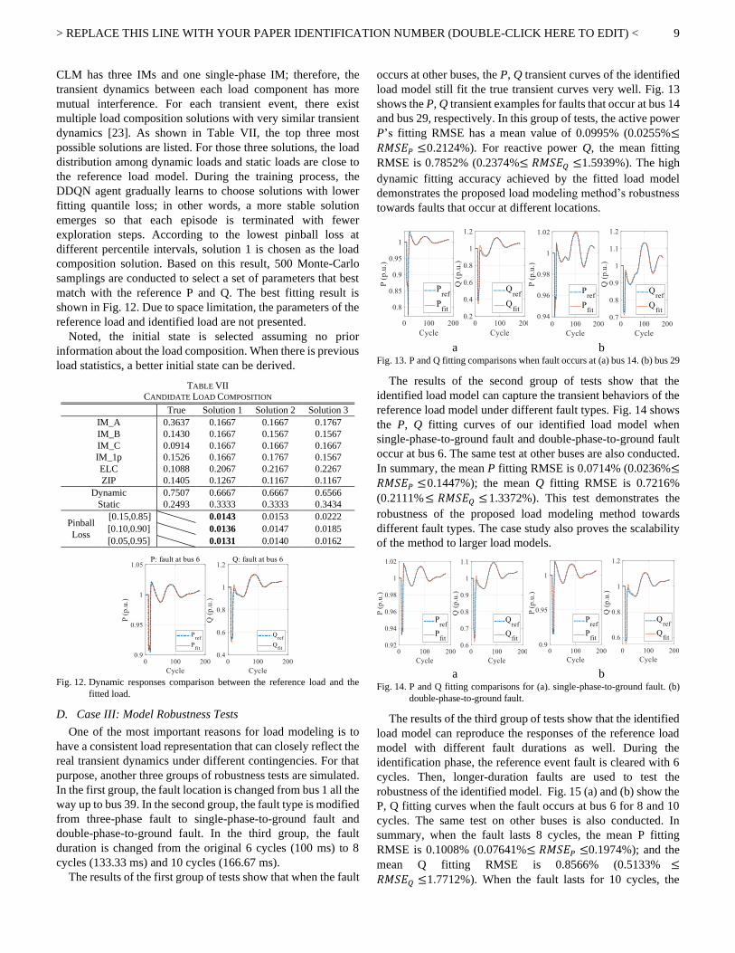
The results of the first group of tests show that when the fault

occurs at other buses, the P, Q transient curves of the identified

load model still fit the true transient curves very well. Fig. 13

shows the P, Q transient examples for faults that occur at bus 14

and bus 29, respectively. In this group of tests, the active power

P’s fitting RMSE has a mean value of 0.0995% (0.0255%≤𝑅𝑀𝑆𝐸𝑃 ≤0.2124%). For reactive power Q, the mean fitting

RMSE is 0.7852% (0.2374%≤ 𝑅𝑀𝑆𝐸𝑄 ≤1.5939%). The high

dynamic fitting accuracy achieved by the fitted load model

demonstrates the proposed load modeling method’s robustness

towards faults that occur at different locations.

a b

Fig. 13. P and Q fitting comparisons when fault occurs at (a) bus 14. (b) bus 29

The results of the second group of tests show that the

identified load model can capture the transient behaviors of the

reference load model under different fault types. Fig. 14 shows

the P, Q fitting curves of our identified load model when

single-phase-to-ground fault and double-phase-to-ground fault

occur at bus 6. The same test at other buses are also conducted.

In summary, the mean P fitting RMSE is 0.0714% (0.0236%≤𝑅𝑀𝑆𝐸𝑃 ≤0.1447%); the mean Q fitting RMSE is 0.7216%

(0.2111%≤ 𝑅𝑀𝑆𝐸𝑄 ≤1.3372%). This test demonstrates the

robustness of the proposed load modeling method towards

different fault types. The case study also proves the scalability

of the method to larger load models.

a b

Fig. 14. P and Q fitting comparisons for (a). single-phase-to-ground fault. (b)

double-phase-to-ground fault.

The results of the third group of tests show that the identified

load model can reproduce the responses of the reference load

model with different fault durations as well. During the

identification phase, the reference event fault is cleared with 6

cycles. Then, longer-duration faults are used to test the

robustness of the identified model. Fig. 15 (a) and (b) show the

P, Q fitting curves when the fault occurs at bus 6 for 8 and 10

cycles. The same test on other buses is also conducted. In

summary, when the fault lasts 8 cycles, the mean P fitting

RMSE is 0.1008% (0.07641%≤ 𝑅𝑀𝑆𝐸𝑃 ≤0.1974%); and the

mean Q fitting RMSE is 0.8566% (0.5133% ≤𝑅𝑀𝑆𝐸𝑄 ≤1.7712%). When the fault lasts for 10 cycles, the


10

mean P fitting RMSE is 0.1804% (0.1236% ≤𝑅𝑀𝑆𝐸𝑃 ≤0.2113%); and the mean Q fitting RMSE is 1.2677%

(0.7323%≤ 𝑅𝑀𝑆𝐸𝑄 ≤1.8522%). The load profiles are well

represented by the identified model, which demonstrates the

robustness of the proposed method towards different fault

durations.

a b

Fig. 15. P and Q fitting comparisons for (a). 8-cycle fault at bus 6. (b) 10-cycle

fault at bus 6.

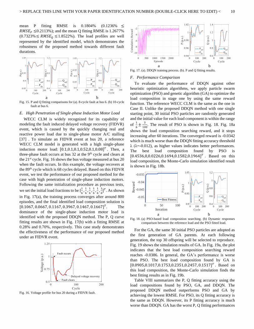
E. High Penetration of Single-phase Induction Motor Load

WECC CLM is widely recognized for its capability of

modeling the fault induced delayed voltage recovery (FIDVR)

event, which is caused by the quickly changing real and

reactive power load due to single-phase motor A/C stalling

[37] . To simulate an FIDVR event at bus 20, a reference

WECC CLM model is generated with a high single-phase

induction motor load: [0.1,0.1,0.1,0.52,0.1,0.08]𝑇 . Then, a

three-phase fault occurs at bus 32 at the 9th cycle and clears at

the 21st cycle. Fig. 16 shows the bus voltage measured at bus 20

when the fault occurs. In this example, the voltage recovers at

the 89th cycle which is 68 cycles delayed. Based on this FIDVR

event, we test the performance of our proposed method for the

case with high penetration of single-phase induction motors.

Following the same initialization procedure as previous tests,

we set the initial load fractions to be [1

6,1

6,1

6,1

6,1

6,1

6]𝑇. As shown

in Fig. 17(a), the training process converges after around 800

episodes, and the final identified load composition solution is

[0.1067, 0.0667, 0.1167, 0.3967, 0.1467, 0.1667]𝑇 . The

dominance of the single-phase induction motor load is

identified with the proposed DDQN method. The P, Q curve

fitting results are shown in Fig. 17(b) with a fitting RMSE at

0.28% and 0.70%, respectively. This case study demonstrates

the effectiveness of the performance of our proposed method

under an FIDVR event.

Fig. 16. Voltage profile for bus 20 during a FIDVR fault.

a b Fig. 17. (a). DDQN training process. (b). P and Q fitting results.

F. Performance Comparison

To evaluate the performance of DDQN against other

heuristic optimization algorithms, we apply particle swarm

optimization (PSO) and genetic algorithm (GA) to optimize the

load composition in stage one by using the same reward

function. The reference WECC CLM is the same as the one in

Case II. Unlike the proposed DDQN method with one single

starting point, 30 initial PSO particles are randomly generated

and the initial value for each load component is within the range

of 1

6±

3

100. The result of PSO is shown in Fig. 18. Fig. 18a

shows the load composition searching reward, and it stops

increasing after 60 iterations. The converged reward is -0.0342

which is much worse than the DDQN fitting accuracy threshold

λ (λ=-0.012), as higher values indicates better performances.

The best load composition found by PSO is

[0.4536,0,0.0226,0.1694,0.1582,0.1964]𝑇 . Based on this

load composition, the Monte-Carlo simulation identified result

is shown in Fig. 18b.

a b

Fig. 18. (a) PSO-based load composition searching. (b) Dynamic responses

comparison between the reference load and the PSO fitted load.

For the GA, the same 30 initial PSO particles are adopted as

the first generation of GA parents. At each following

generation, the top 30 offspring will be selected to reproduce.

Fig. 19 shows the simulation results of GA. In Fig. 19a, the plot

indicates that the best load composition searching reward

reaches -0.0386. In general, the GA’s performance is worse

than PSO. The best load composition found by GA is

[0.0905,0.1017,0.1753,0.2351,0.2457, 0.1517]𝑇 . Based on

this load composition, the Monte-Carlo simulation finds the

best fitting results as in Fig. 19b.

Table VIII summarizes the P, Q fitting accuracy using the

load compositions found by PSO, GA, and DDQN. The

proposed DDQN method outperforms PSO and GA by

achieving the lowest RMSE. For PSO, its Q fitting accuracy is

the same as DDQN. However, its P fitting accuracy is much

worse than DDQN. GA has the worst P, Q fitting performances

0 50 100

Iteration

-0.05

-0.045

-0.04

-0.035

Rew

ard

Best Fitness

0 100 200

Cycle

0.9

0.95

1

1.05

P (

p.u

.)

Pref

Pfit

0 100 200

Cycle

0.4

0.6

0.8

1

1.2

Q (

p.u

.)

Qref

Qfit


11

in this case. Since the second-stage parameter identification

follows the same procedure for these three methods, this

comparison also partially verifies our claims in Section II that

identifying a proper load composition can greatly improve the

dynamic response reconstruction efficiency.

a b Fig. 19. (a) GA-based load composition searching. (b) Dynamic responses

comparison between the reference load and the GA fitted load.

TABLE VIII PERFORMANCE COMPARISON

PSO GA DDQN

RMSE for P 0.0050 0.0075 0.0012

RMSE for Q 0.0065 0.0358 0.0064

We conducted other two groups of comparison between PSO,

GA, and DDQN, the results consistently show that DDQN’s

performance are better than PSO and GA, and PSO’s

performance is better than GA. This comparison also verifies

our claims in Section II, that identifying a proper load

composition can greatly improve the parameter fitting

efficiency.

G. Impact of Initial Point on the Algorithm Performance

The proposed load modeling method nonlinearly optimizes

the load compositions. It is critical to evaluate the impacts of

the initial point selection on the identification results. In this

section, we design another WECC CLM with a reference load

composition as 𝒔𝑊𝐸𝐶𝐶 = [0.1,0.15,0.1,0.2,0.1,0.35]T. Then we

conduct the two load modeling tests, Test-Rand and Test-Close,

using two different initial points. The initial point for

Test-Rand is the same as the Case II, which is [1/6, 1/6, 1/6, 1/6,

1/6, 1/6]T. The initial point for Test-Close is designed to be very

close to the reference load composition, which is

[0.08,0.1,0.13,0.22,0.07,0.4]T. By comparing Test-Rand with

Test-Close, we can evaluate the impacts of different initial

points on the same case. TABLE IX

PERFORMANCE COMPARISON

True Test-Rand Test-Close

Stage one

IM_A 0.1000 0.0967 0.0900

IM_B 0.1500 0.1667 0.1500

IM_C 0.1000 0.1667 0.0800

IM_1p 0.2000 0.1467 0.2100

ELC 0.1000 0.1667 0.0700

ZIP 0.3500 0.2567 0.4000

Static Load 0.4500 0.4234 0.4700

Dynamic Load 0.5500 0.5766 0.5300

Pinball Loss

0.0134 0.0125

Stage two P fitting RMSE 0.0011 0.0013

Q fitting RMSE 0.0046 0.0019

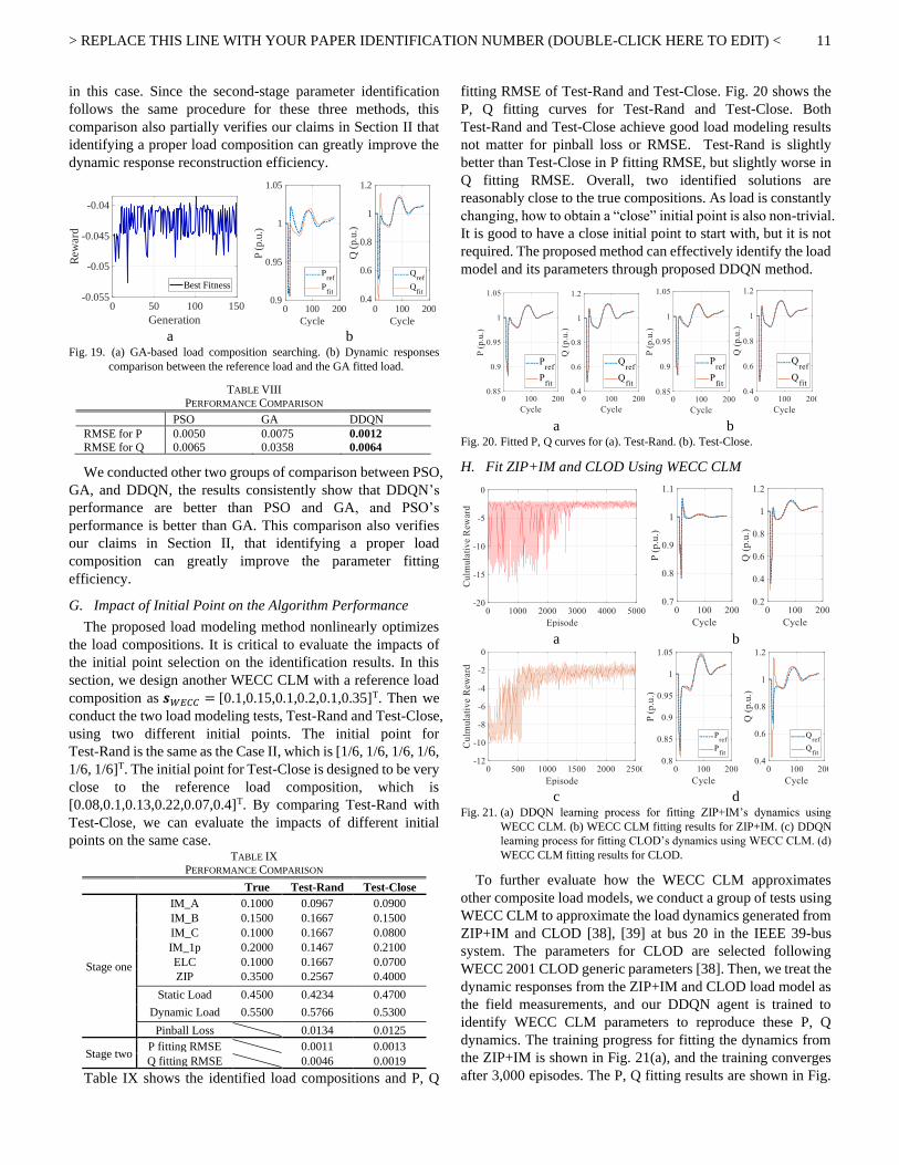
Table IX shows the identified load compositions and P, Q

fitting RMSE of Test-Rand and Test-Close. Fig. 20 shows the

P, Q fitting curves for Test-Rand and Test-Close. Both

Test-Rand and Test-Close achieve good load modeling results

not matter for pinball loss or RMSE. Test-Rand is slightly

better than Test-Close in P fitting RMSE, but slightly worse in

Q fitting RMSE. Overall, two identified solutions are

reasonably close to the true compositions. As load is constantly

changing, how to obtain a “close” initial point is also non-trivial.

It is good to have a close initial point to start with, but it is not

required. The proposed method can effectively identify the load

model and its parameters through proposed DDQN method.

a b Fig. 20. Fitted P, Q curves for (a). Test-Rand. (b). Test-Close.

H. Fit ZIP+IM and CLOD Using WECC CLM

a b

c d Fig. 21. (a) DDQN learning process for fitting ZIP+IM’s dynamics using

WECC CLM. (b) WECC CLM fitting results for ZIP+IM. (c) DDQN

learning process for fitting CLOD’s dynamics using WECC CLM. (d)

WECC CLM fitting results for CLOD.

To further evaluate how the WECC CLM approximates

other composite load models, we conduct a group of tests using

WECC CLM to approximate the load dynamics generated from

ZIP+IM and CLOD [38], [39] at bus 20 in the IEEE 39-bus

system. The parameters for CLOD are selected following

WECC 2001 CLOD generic parameters [38]. Then, we treat the

dynamic responses from the ZIP+IM and CLOD load model as

the field measurements, and our DDQN agent is trained to

identify WECC CLM parameters to reproduce these P, Q

dynamics. The training progress for fitting the dynamics from

the ZIP+IM is shown in Fig. 21(a), and the training converges

after 3,000 episodes. The P, Q fitting results are shown in Fig.

0 50 100 150

Generation

-0.055

-0.05

-0.045

-0.04

Rew

ard

Best Fitness

0 100 200

Cycle

0.9

0.95

1

1.05

P (

p.u

.)

Pref

Pfit

0 100 200

Cycle

0.4

0.6

0.8

1

1.2

Q (

p.u

.)

Qref

Qfit


12

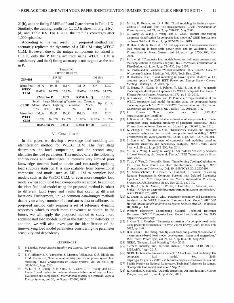
21(b), and the fitting RMSE of P and Q are shown in Table IIX.

Similarly, the training results for CLOD is shown in Fig. 21(c),

(d) and Table IIX. For CLOD, the training converges after

1,000 episodes.

According to the test result, our proposed method can

accurately replicate the dynamics of a ZIP+IM using WECC

CLM. However, due to the unique components contained in

CLOD, only the P fitting accuracy using WECC CLM is

satisfactory, and the Q fitting accuracy is not as good as the one

in P. TABLE IIX

FITTING RESULTS

ZIP+IM ZIP (%) IM (%)

60 40

Identified:

WECC

CLM

IM_A IM_B IM_C IM_D ZIP ELC

18.67% 16.67% 16.67% 16.67% 16.67% 14.67%

RMSE for P: 0.0074 RMSE for Q: 0.0161

CLOD

Small

Motor

Large

Motor

Discharging

Lighting

Transformer

Saturation

Constant

MVA Kp R X

10% 10% 0% 0% 0% 1 0 0

Identified:

WECC

CLM

IM_A IM_B IM_C IM_D ZIP ELC

1.67% 16.67% 15.67% 16.67% 32.67% 16.67%

RMSE for P: 0.0035 RMSE for Q: 0.0611

V. CONCLUSIONS

In this paper, we develop a two-stage load modeling and

identification method for WECC CLM. The first stage

determines the load composition, and the second stage

identifies the load parameters. This method offers the following

contributions and advantages: it requires very limited prior

knowledge towards hard-to-obtain and constantly updating

load structure statistics. It is also scalable, from conventional

composite load model such as ZIP + IM to complex load

models such as the WECC CLM, or even more complex load

models when additional load components are added. In addition,

the identified load model using the proposed method is robust

to different fault types and faults that occur at different

locations. Furthermore, unlike common data-hungry methods

that rely on a large number of disturbances data to calibrate, the

proposed method only requires a set of reference dynamic

responses, which is much more convenient to obtain. In the

future, we will apply the proposed method to study more

sophisticated load models, such as the distribution networks. In

addition, we will also investigate the identification of the

time-varying load model parameters considering the parameter

sensitivity and dependency.

REFERENCES

[1] P. Kundur, Power System Stability and Control. New York: McGrawHill,

1993.

[2] J. V. Milanovic, K. Yamashita, S. Martínez Villanueva, S. Ž. Djokic and L. M. Korunović, “International industry practice on power system load

modeling,” IEEE Transactions on Power Systems, vol. 28, no. 3, pp.

3038-3046, Aug. 2013. [3] Y. Li, H.-D. Chiang, B.-K. Choi, Y.-T. Chen, D.-H. Huang, and M.G.

Lauby, “Load models for modeling dynamic behaviors of reactive loads:

Evaluation and comparison,” International Journal of Electrical Power & Energy Systems, vol. 30, no. 9, pp. 497-503, 2008.

[4] M. Jin, H. Renmu, and D. J. Hill, “Load modeling by finding support

vectors of load data from field measurements,” IEEE Transactions on Power Systems, vol. 21, no. 2, pp. 726-735, May 2006.

[5] C. Wang, Z. Wang, J. Wang, and D. Zhao, “Robust time-varying

parameter identification for composite load modelin,” IEEE Transactions

on Smart Grid, vol. 10, no. 1, pp. 967-979, Jan. 2019.

[6] D. Han, J. Ma, R. He et al., “A real application of measurement-based

load modeling in large-scale power grids and its validation,” IEEE

Transactions on Power Systems, vol. 24, no. 4, pp. 1756-1764, Nov.

2009. [7] P. Ju et al., “Composite load models based on field measurements and

their applications in dynamic analysis,” IET Generation, Transmission &

Distribution, vol. 1, no. 5, pp. 724-730, Sep. 2007. [8] A. Borden and B. Lesieutre, “Model validation: FIDVR event,” Univ. of

Wisconsin-Madison, Madison, WI, USA, Tech. Rep., 2009.

[9] D. Kosterev et al., "Load modeling in power system studies: WECC progress update," in 2008 IEEE Power and Energy Society General

Meeting, Pittsburgh, PA, 2008, pp. 1-8.

[10] Q. Huang, R. Huang, B. J. Palmer, Y. Liu, S. Jin, et al., "A generic modeling and development approach for WECC composite load model, "

Electric Power Systems Research, vol. 172, pp 1-10, 2019.

[11] A. Gaikwad, P. Markham, and P. Pourbeik, "Implementation of the WECC composite load model for utilities using the component-based

modeling approach," in 2016 IEEE/PES Transmission and Distribution

Conference and Exposition (T&D), Dallas, TX, 2016, pp. 1-5. [12] P. Etingov, "Load model data tool (LMDT),"

https://svn.pnl.gov/LoadTool.

[13] J. Kim et al., "Fast and reliable estimation of composite load model parameters using analytical similarity of parameter sensitivity," IEEE

Transactions on Power Systems, vol. 31, no. 1, pp. 663-671, Jan. 2016.

[14] K. Zhang, H. Zhu, and S. Guo, "Dependency analysis and improved parameter estimation for dynamic composite load modeling," IEEE

Transactions on Power Systems, vol. 32, no. 4, pp. 3287-3297, Jul. 2017.

[15] S. Son et al., “Improvement of composite load modeling based on parameter sensitivity and dependency analyses,” IEEE Trans. Power

Syst., vol. 29, no. 1, pp. 242–250, Jan. 2014. [16] Y. Lin, Y. Wang, J. Wang, S. Wang, D. Shi, “Global Sensitivity Analysis

in Load Modeling via Low-rank Tensor,” IEEE Transactions on Smart

Grid, 2020. [17] Y. Li, Y. Wen, D. Tao and K. Guan, “Transforming Cooling Optimization

for Green Data Center via Deep Reinforcement Learning,” IEEE

Transactions on Cybernetics. Doi: 10.1109/TCYB.2019.2927410. [18] M. Schaarschmidt, F. Gessert, V. Dalibard, E. Yoneki, “Learning

Runtime Parameters in Computer Systems with Delayed Experience

Injection,” in 2016 Conference on Neural Information Processing Systems (NIPS), Barcelona, Spain, Dec. 2016, pp. 1-10.

[19] A. Haj-Ali, N. K. Ahmed, T. Willke, J. Gonzalez, K. Asanovic, and I.

Stoica, “A view on deep reinforcement learning in system optimization,” arXiv:1908.01275, 2019.

[20] K. Zhang, S. Guo, and H. Zhu. "Parameter Sensitivity and Dependency

Analysis for the WECC Dynamic Composite Load Model," 2017 50th Hawaii International Conference on System Sciences (HICSS), Waikoloa,

HI, 2016, pp. 1-8.

[21] Western Electricity Coordinating Council, Technical Reference Document: "WECC Composite Load Model Specifications" Jan. 2015,

https://www.wecc.org/

[22] S. Guo, T. J. Overbye, “Parameter estimation of a complex load model using phasor measurements,” in Proc. Power Energy Conf., Illinois, Feb.

2012, pp. 1–6.

[23] B. K. Choi, H. D. Chiang, “Multiple solutions and plateau phenomenon in measurement-based load model development: Issues and suggestions,”

IEEE Trans. Power Syst., vol. 24, no. 2, pp. 824-831, May 2009.

[24] NERC, "Dynamic Load Modeling," Nov. 2016. [25] Siemens Industry, Inc, software manual: "PSS®E 33.10, MODEL

LIBRARY, " Apr. 2017.

[26] NERC Technical Reference Document: " A Look into load modeling: The composite load model." Sep. 2015,

https://gig.lbl.gov/sites/all/files/6b-quint-composite-load-model-data.pdf

[27] Pacific Northwest National Laboratory, Technical Reference Document: "Composite load model evaluation," Sep. 2015.

[28] R. Koenker, K. Hallock, "Quantile regression: An introduction", J. Econ.

Perspectives, vol. 15, no. 4, pp. 43-56, 2001.


13

[29] Q. Chang, Y. Wang, X. Lu et al., "Probabilistic Load Forecasting via

Point Forecast Feature Integration," in 2019 IEEE Innovative Smart Grid Technologies - Asia (ISGT Asia), Chengdu, China, 2019, pp. 99-104.

[30] J. Duan, H. Xu and W. Liu, “Q-Learning-Based Damping Control of

Wide-Area Power Systems Under Cyber Uncertainties,” IEEE Transactions on Smart Grid, vol. 9, no. 6, pp. 6408-6418, Nov. 2018.

[31] J. Duan, Z. Yi, D. Shi, C. Lin, X. Lu and Z. Wang,

“Reinforcement-Learning-Based Optimal Control of Hybrid Energy Storage Systems in Hybrid AC–DC Microgrids,” IEEE Transactions on

Industrial Informatics, vol. 15, no. 9, pp. 5355-5364, Sep. 2019.

[32] J. Duan, D. Shi et al., "Deep-Reinforcement-Learning-Based Autonomous Voltage Control for Power Grid Operations," IEEE

Transactions on Power Systems, vol. 35, no. 1, pp. 814-817, Jan. 2020.

[33] H. V. Hasselt, A. Guez, and D. Silver, “Deep reinforcement learning with double Q-learning,” arXiv:1509.06461,2016.

[34] I. Durugkar and P. Stone, “TD learning with constrained gradients,” in

Proc. of the Deep Reinforcement Learning Symposium (NIPS 2017), Long Beach, CA, USA December 2017.

[35] R. Liu and J. Zou, “The effects of memory replay in reinforcement

learning,” The ICML 2017 Workshop on Principled Approaches to Deep

Learning, Sydney, Australia, 2017.

[36] P. Cicilio and E. Cotilla-Sanchez, "Evaluating Measurement-Based

Dynamic Load Modeling Techniques and Metrics," IEEE Transactions on Power Systems, 2019.

[37] R. J. Bravo, R. Yinger and P. Arons, “Fault Induced Delayed Voltage

Recovery (FIDVR) Indicators,” 2014 IEEE PES T&D Conference and Exposition, Chicago, IL, 2014, pp. 1-5.

[38] A. S. Hoshyarzadeh, H. Zareipour, P. Keung, and S. S. Ahmed, “The

Impact of CLOD Load Model Parameters on Dynamic Simulation of Large Power Systems,” in 2019 IEEE International Conference on

Environment and Electrical Engineering and 2019 IEEE Industrial and

Commercial Power Systems Europe (EEEIC / I&CPS Europe), Genova, Italy, 2019, pp. 1-6.

[39] S. Li, X. Liang and W. Xu, “Dynamic load modeling for industrial

facilities using template and PSS/E composite load model structure CLOD,” in 2017 IEEE/IAS 53rd Industrial and Commercial Power

Systems Technical Conference (I&CPS), Niagara Falls, ON, 2017, pp.

1-9.

Xinan Wang (S’15) received the B.S. degree from Northwestern Polytechnical University, Xi’an, China,

in 2013, and the M.S. degree from Arizona State

University, Tempe, AZ, USA, in 2016, both in electrical engineering. He was a Research Assistant in

the AI & System Analytics Group at GEIRI North

America, San Jose, CA, in 2016, 2017 and 2019. He is currently pursuing the Ph.D. degree with the

Department of Electrical and Computer Engineering at Southern Methodist University, Dallas, Texas, USA.

His research interests include machine learning applications to power systems,

wide-area measurement systems, data analysis and load modeling.

Yishen Wang (S’13–M’17) received the B.S. degree in

electrical engineering from Tsinghua University,

Beijing, China, in 2011, the M.S. and the Ph.D. degree in electrical engineering from the University of

Washington, Seattle, WA, USA, in 2013 and 2017,

respectively. He is currently a Power System Research Engineer with GEIRI North America, San Jose, CA,

USA. His research interests include load modeling,

PMU data analytics, power system economics and operation, energy storage, and microgrids.

Di Shi (M’12–SM’17) received the Ph.D. degree in

electrical engineering from Arizona State University.

He is currently the Department Head of the AI & System Analytics Group, Global Energy

Interconnection Research Institute North America

(GEIRINA), San Jose, CA, USA. Prior to joining GEIRINA, He was a Research Staff Member with NEC

Laboratories America. His research interests include PMU data analytics, AI,

energy storage systems, the IoT for power systems, and renewable integration.

He is an Editor of the IEEE Transactions on Smart Grid and the IEEE Power

Engineering Letters.

Jianhui Wang (M’07-SM’12). Dr. Jianhui Wang is an

Associate Professor with the Department of Electrical

and Computer Engineering at Southern Methodist

University. Dr. Wang has authored and/or co-authored

more than 300 journal and conference publications,

which have been cited for more than 20,000 times by

his peers with an H-index of 68. He has been invited to

give tutorials and keynote speeches at major

conferences including IEEE ISGT, IEEE

SmartGridComm, IEEE SEGE, IEEE HPSC and

IGEC-XI.

Dr. Wang is the past Editor-in-Chief of the IEEE Transactions on Smart Grid

and an IEEE PES Distinguished Lecturer. He is also a guest editor of a

Proceedings of the IEEE special issue on power grid resilience. He is the

recipient of the IEEE PES Power System Operation Committee Prize Paper

Award in 2015 and the 2018 Premium Award for Best Paper in IET

Cyber-Physical Systems: Theory & Applications. Dr. Wang is a 2018 and 2019

Clarivate Analytics highly cited researcher for production of multiple highly

cited papers that rank in the top 1% by citations for field and year in Web of

Science.

Zhiwei Wang (M’16-SM’18) received the B.S. and

M.S. degrees in electrical engineering from Southeast

University, Nanjing, China, in 1988 and 1991, respectively. He is President of GEIRI North America,

San Jose, CA, USA. Prior to this assignment, he served

as President of State Grid US Representative Office,

New York City, from 2013 to 2015, and President of

State Grid Wuxi Electric Power Supply Company from

2012-2013. His research interests include power system operation and control, relay protection, power system planning, and WAMS.

Documents

stage WECC Composite Load Modeling: A Double Deep Q ... WECC Composite Load Modeling.pdfDouble Deep Q-Learning Networks Approach A This work is funded by SGCC Science and Technology