Staffing Service Systemsvia

Simulation

Julius Atlason, Marina Epelman

University of Michigan

Shane Henderson

Cornell University

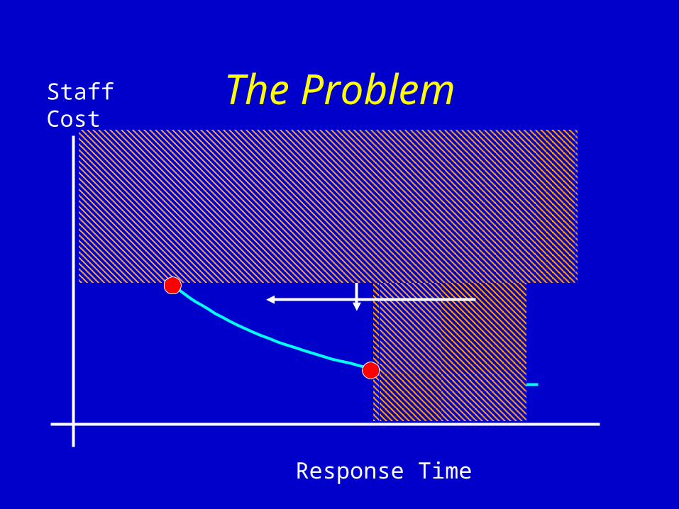
The Problem

Response Time

Staff Cost

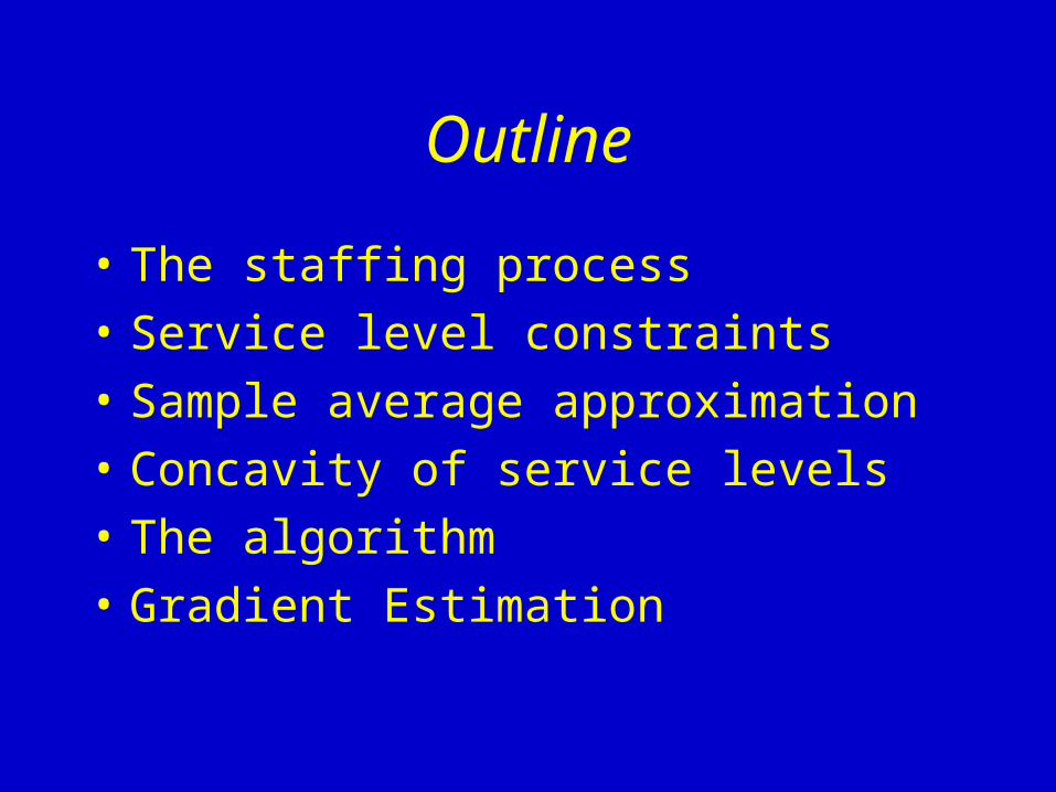
Outline

• The staffing process

• Service level constraints

• Sample average approximation

• Concavity of service levels

• The algorithm

• Gradient Estimation

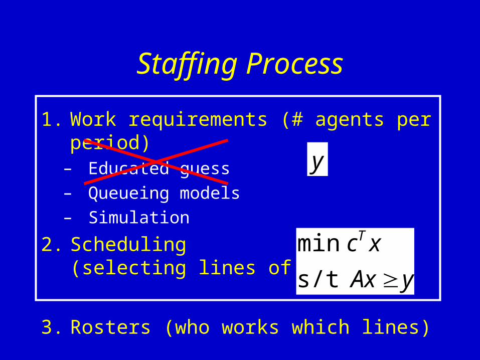
Staffing Process

1. Work requirements (# agents per period)– Educated guess– Queueing models– Simulation

2. Scheduling(selecting lines of work)

3. Rosters (who works which lines)

yAx

xcT

s/t

min

y

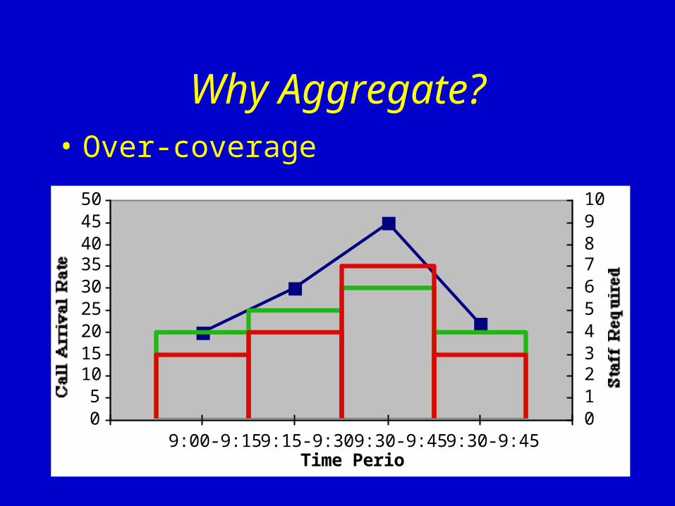
Why Aggregate?• Over-coverage

05

101520253035404550

9:00-9:15 9:15-9:30 9:30-9:45 9:30-9:45Time Period

012345678910

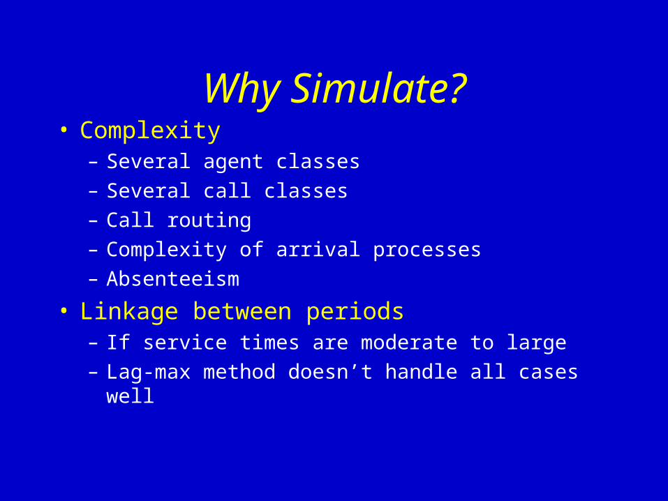
Why Simulate?• Complexity

– Several agent classes

– Several call classes

– Call routing

– Complexity of arrival processes

– Absenteeism

• Linkage between periods– If service times are moderate to large

– Lag-max method doesn’t handle all cases well

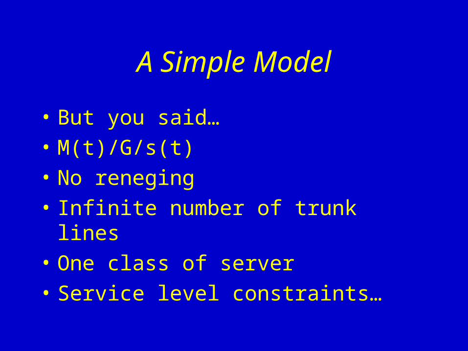
A Simple Model

• But you said…

• M(t)/G/s(t)

• No reneging

• Infinite number of trunk lines

• One class of server

• Service level constraints…

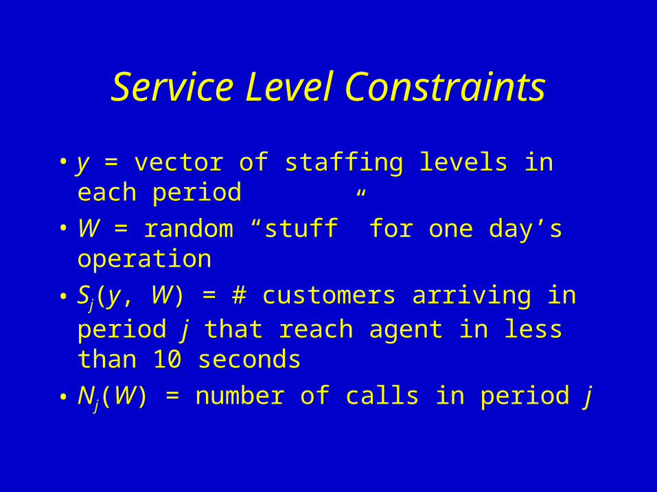
Service Level Constraints

• y = vector of staffing levels in each period

• W = random “stuff” for one day’s operation

• Sj(y, W) = # customers arriving in period j that reach agent in less than 10 seconds

• Nj(W) = number of calls in period j

Service Level Constraints

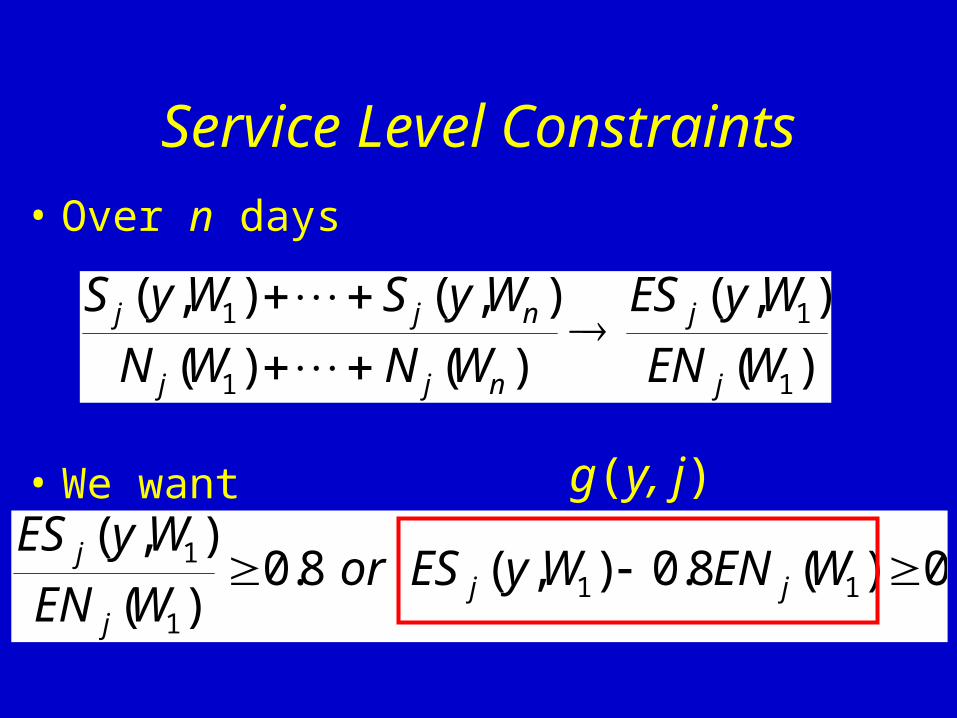
• Over n days

• We want

)(

),(

)()(

),(),(

1

1

1

1

WEN

WyES

WNWN

WySWyS

j

j

njj

njj

0)(8.0),(8.0)(

),(11

1

1 WENWyESorWEN

WyESjj

j

j

g(y, j)

Sample Average Approximation

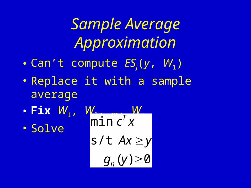
• Can’t compute ESj(y, W1)

• Replace it with a sample average

• Fix W1, W2, …, Wn

• Solve

0)(

s/t

min

yg

yAx

xc

n

T

Sample Average Approximation

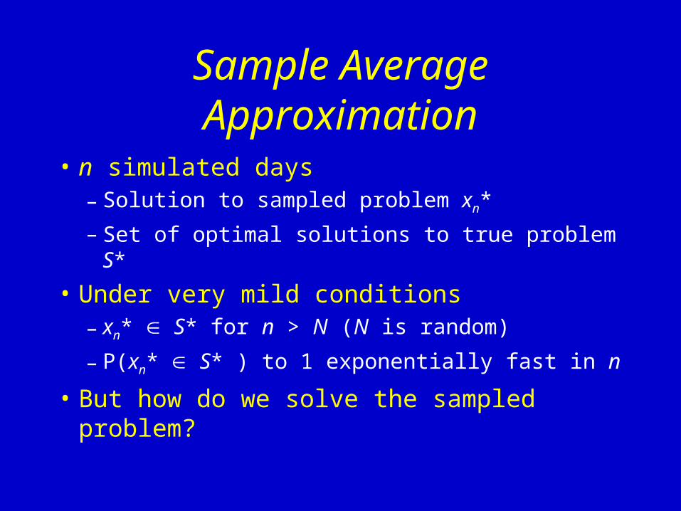
• n simulated days– Solution to sampled problem xn*

– Set of optimal solutions to true problem S*

• Under very mild conditions– xn* S* for n > N (N is random)

– P(xn* S* ) to 1 exponentially fast in n

• But how do we solve the sampled problem?

Concavity of the Service Levels

• Want g(y) 0

• g is nondecreasing

• g is concave in each component?

• g is jointly concave?

• Checked numerically in our algorithm

• But does it hold?

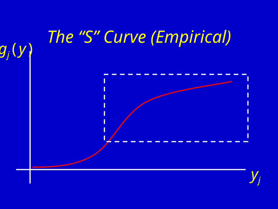
The “S” Curve (Empirical)

yj

gj(y)

Cutting Planes

g(y) 0g(y*)+ G(y*)T(y – y*)

cuts (linear)

s/t

min

yAx

xcT

g(y*)+ G(y*)T(y – y*) 0

“Solve” IP Simulate

y

cuts

Converges in finite # iterations

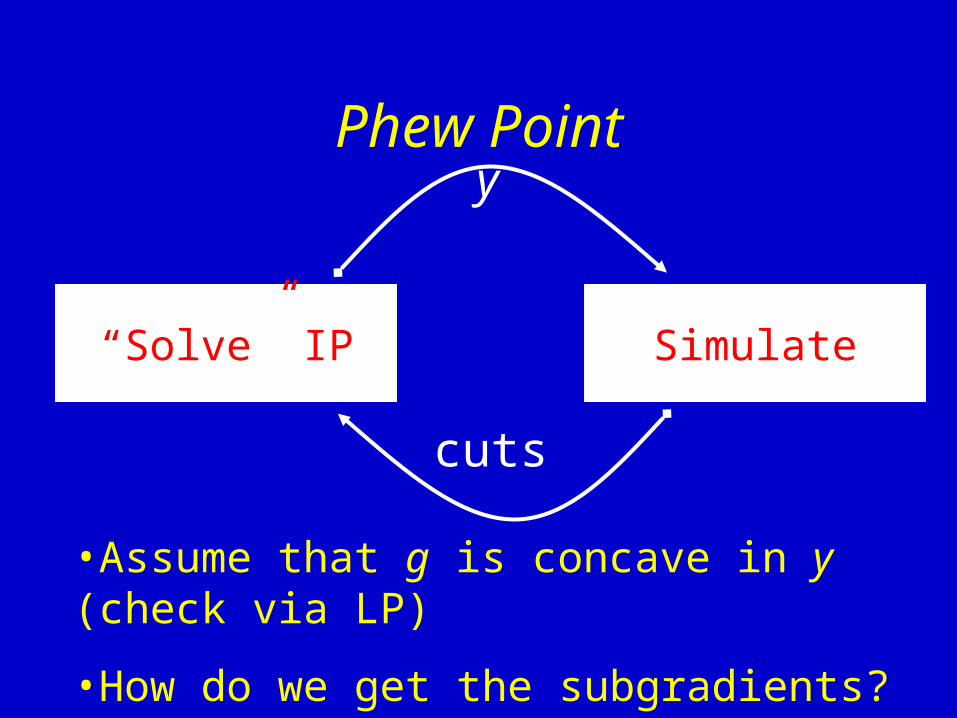
Phew Point

“Solve” IP Simulate

y

cuts

•Assume that g is concave in y (check via LP)

•How do we get the subgradients?

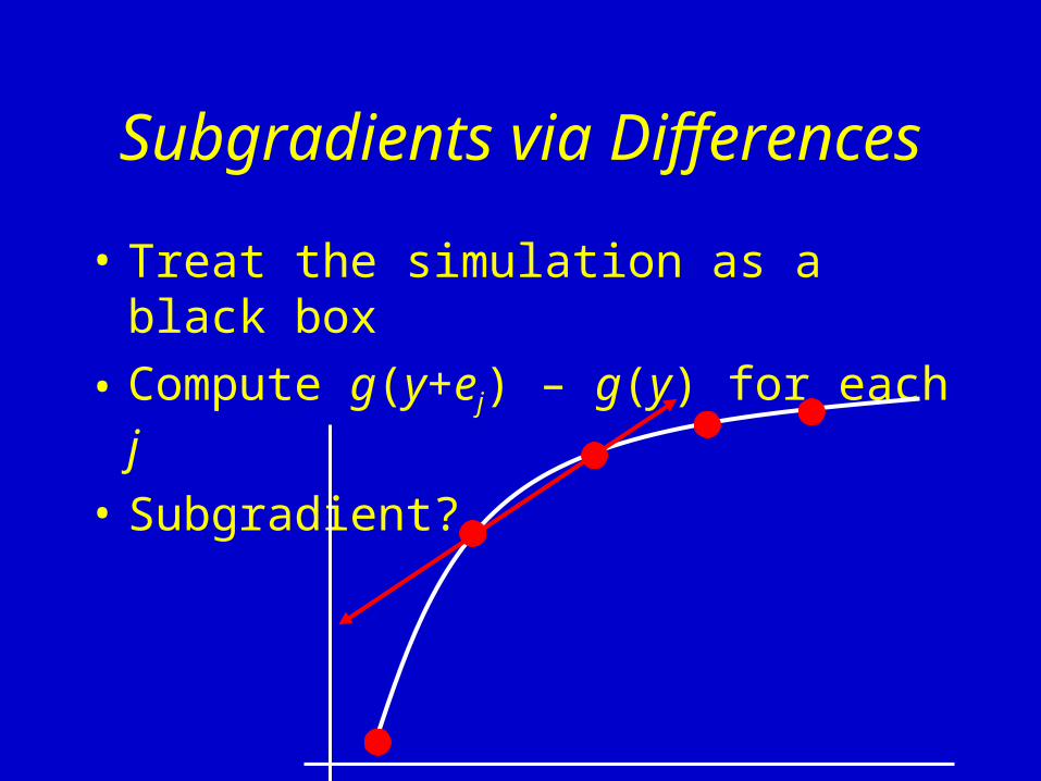
Subgradients via Differences

• Treat the simulation as a black box

• Compute g(y+ej) – g(y) for each j

• Subgradient?

Estimating Subgradients: IPA

• IPA (smoothed) differentiates sample path

• But servers are discrete

• Use service rate as a proxy for # servers

• Need #servers fixed over entire horizon to ensure interchange is ok!

• Vary service rate with period to match true service capacity

Estimating Subgradients: LR

• Lots of heuristics with smoothed IPA

• Likelihood ratio (score function) method?

• Seems to apply more easily, but still some less-than-ideal modeling assumptions

• Overall: subgradient estimation unresolved

Some Computational Results

• Only (very) small problems thus far

• Requires very few iterations

• Differencing seems to work!

• Smoothed IPA, LR: Jury still out

Summary To Date

• Very few iterations are needed to “zero in” on good staffing levels

• Have convergence theory both for fixed n, and as n increases

• Subgradient estimation remains a challenge

• Working with Ann Arbor Police on patrol car staffing

Future Research

• Concavity, S curves

• Why does differencing work?

• Can we relax concavity assumption to quasiconcavity (modify algorithm)?

• Integer programming takes a while…