Stabilization of a Quadrotor using Image-based

Processing

Romeu Paulo Santos Chumbo ∗

∗Department of Mechanical Engineering - IDMEC, Instituto SuperiorTecnico, Technical University of Lisbon (TULisbon) Av. Rovisco Pais,

1049-001 Lisboa, Portugal; e-mail: romeu.chumbo@ist.utl.pt

Abstract:The control of the horizontal position of a quadrotor when in hovering, requires the observationof the translation. One of the possible solutions is the use of GPS, but its accuracy is unsatisfying.It is thus necessary to develop a solution that warrants enough accuracy.This work develops an image-based control strategy. It places a camera under the quadrotortowards the ground, which identifies the UAV motion using image tracking. The result is thenintegrated into a cascade controller, regulating its position back to the original pose.Two LQR controllers are projected and simulation-validated, one for each loop in the cascadecontrol. Then, we proceed to the integration of the homography-based position control, testingfor multiple values of image resolution and vision angles.Once the control method is validated, the image tracking algorithm is implemented in Matlab.This algorithm searches the reference image over a video sequence, and returns the homographywhich expresses the motion.After program optimization, the speed was still not enough. For this reason, and because theSRV-1 requires a C implementation, the program is converted into that language first on aPC platform. The C code performs the real-time tracking up to 30Hz. Then, the programperformance is tested using multiple types of image patterns.The algorithm was ported on the SRV-1 but the resulting processing rate of 0.17Hz is far belowthe 5Hz limit that was necessary for the position control. For this reason, the projected controlwas not taken to implementation on the UAV.

Keywords: Quadrotor, Image Tracking, Visual Servoing, Real Time Control.

1. INTRODUCTION

This work was suggested by the company UAVision, whichis developing a quadrotor, and needed an additional con-trol system. The quadrotor is quipped with:

• Self stabilization with an IMU, compass and baro-metric height sensor• Take-off and landing in automatic mode• Autonomous navigation with GPS• Control from a ground station and real-time image

transmission

However, when in hovering, the quadrotor drifts in thehorizontal plane. This can be caused by multiple reasons(side wind, small accuracy of the IMU data, small accu-racy in the actuation, noise, among others). This work isproposed to solve this problem, coming up with an image-based solution which regulates the position, avoiding un-desired movements. For the implementation, UAVision hasavailable the DSP micro controller surveyor SRV-1, whichallows the image processing directly from a camera. Weneeded to execute each of the following steps:

(1) Design of a horizontal translation controller for thequadrotor

(2) Simulation of the controller with homography-feedback

(3) Development, validation and test of the image-tracking algorithm

(4) Implementation of the tracking algorithm in C, notonly on PC but also on SRV-1

(5) Integration of SRV-1 into the quadrotor, validatingthe projected controller

This article is organized as follows: in section 2, a briefstate of the art about quadrotors and image tracking is pre-sented; in section 3 the model of quadrotor is introducedas well as the control design; in section 3 the homography-based control is integrated as an outer loop for horizontalposition control and the close loop behavior is studied;in section 4 the image-tracking algorithm is introduced,implemented in Matlab and its performance is evaluatedagainst the configuration parameters. It is then imple-mented in C language exhibiting real time performance;in a final section, the main conclusions of this work arepresented as well as some suggestions for the next steps ofthe project.

2. STATE OF THE ART

2.1 Quadrotor

The quadrotor concept began in the beginning of theXX century, when in 1907 Louis and Jacques Breguet

developed the ”Gyroplane No.1” [aviastar, 2011]. Recently,the development in technology and electronics, the appear-ing of sensors and miniature microprocessors allowed theconstruction of smaller quadrotors, light and economicallyaccessible, where it is possible to implement and developoriginal solutions, allowing new scientific achievements.

2.2 Visual Servoing

Visual servoing is also known as Visual Servo Control. Ituses the visual information to control the position of arobot relatively to a target or a set of target-characteristics[Corke, 1994]. In literature the visual servoing methods arein general classified as follows, according to its trajectory:

• 3D visual servoing (PBVS): the task is expressed inCartesian space, i.e. the information obtained fromtwo images (using reference image and current image)is used explicitly to rebuild the position and attitudeof a camera [Wilson et al., 1996], [Basri et al., 1998],[Taylor and Ostrowski, 2000] e [Malis and Chaumette,2002].• 2D visual servoing (IBVS): This method does not

need of the explicit prediction of position’s error inCartesian space [Espiau et al., 1992] [Chaumette,2004], because it builds an isomorphic task for thecamera’s position.• 2D 1/2 visual servoing : the path is expressed from

the image Cartesian space, i.e. the rotation errorof estimated explicitly, and the translation error isexpress from the image.

Where PBVS and IBVS stand for Position-Based VisualServoing and Image-Based Visual Servoing, defined by[Sanderson and Weiss, 1980]. The solution used here for thecontrol of a quadrotor is based on [BenHimane and Malis,2007]. It is a 3D visual servoing method that controlsthe robot control building an isomorphic path for cameraposition in the Cartesian space, based on homography.

Image tracking Image tracking is the process to findand track a reference image along a sequence of imagesor video, through image analysis. It is classified in twomain groups [BenHimane and Malis, 2007]. The first iscomposed by methods which search features, such asline segments or contours [Isard and Blake, 1996], [Torrand Zisserman, 2000], [Drummond and Cipolla, 1999].The second group contains the methods which use theinformation relative to the image intensity.

[BenHimane and Malis, 2004] proposes the use of anEfficient Second-Order Minimization. The ESM uses anhomography to identify the relation between two pictures.In 2010, [Tahri and Mezouar, 2010] proposes a variantbased in ESM method, where he changes the method tominimize the cost function. The approach in this work usesnot only the ESM and Tahri method, but also the simpleJacobian method for image tracking.

3. MODELING THE PROBLEM AND CONTROLLERDESIGN

The solution we are looking for integrates control andimage processing. In this part it is presented the control

solution. In the following one, we expose the image-processing solution and integration.

The UAV open-loop dynamic model is introduced throughthe dynamics equations, and the variables which makeit. The next step is the construction of the model andlinearization about the equilibrium point, allowing us tohave a linearized model of the UAV. The low-level controlstabilizes the attitude and height, the existent sensorsin the UAVision model.The high-level controller controlsthe horizontal translation through image feedback. Thisfeedback is made using the homography.

3.1 Quadrotor

In this work we define two frames, the inertial (or fixed)frame and the UAV frame, shown in figure 1.

((a)) Inertial frame (NED) ((b)) Quadrotor frame

Fig. 1. Example of quadrotor and frames used (from[Henriques, 2011])

The rotation matrix from equation 1 presents the rota-tion from the earth fix frame (the North-East-Down orNED frame) to the UAV body frame.. This matrix isthe successive multiplication of three elementary rotationmatrices (R), one for each Euler angle, as follows: S =R(φ)R(θ)R(ψ).

S =

[cψ cθ cθ sψ −sθ

cψ sφ sθ − cφ sψ cφ cψ + sφ sψ sθ cθ sφsφ sψ + cφ cψ sθ cφ sψ sθ − cψ sφ cφ cθ

](1)

The kinematic equations of the quadrotor are:

p = [x, y, z]T (2)

V = [U, V, W ]T (3)

Ψ = [φ, θ, ψ]T (4)

Ω = [P, Q, R]T (5)

where p is the position of the quadrotor in the NED frame,V is the linear speed of the quadrotor in the body frame,Ψ are the Euler angles, and Ω is the angular speed in thebody frame.

3.2 Dynamic Model

From Newton’s second law, we have the following equa-tions for dynamics:

m(V + Ω×V) = F

I(Ω + Ω× IΩ) = M(6)

where m is the quadrotor mass, I is the quadrotor inertiamatrix, F and M are the total force and moments appliedto the quadrotor. The position and attitude of the quadro-tor in the NED frame is given by the cinematic equations:

p =ST V

Ψ =Rt Ω(7)

The propulsion forces in UAV frame are the following:

Fz =− b (W 21 +W 2

2 +W 23 +W 2

4 )

Fm =[0 0 Fz]T

Mx =b (W 24 −W 2

2 ) l

My =b (W 21 −W 2

3 ) l

Mz =d

2(W 2

2 +W 24 −W 2

3 −W 21 )

Mm =[Mx My Mz]T

(8)

where Wi is the speed of motor i, Fz is the thrust force, Fmis the total force due to motors propulsion and Mm is theresultant moment due to motor’s action. The constants be d are respectively the propeller propulsion and torquecoefficients. The aerodynamic forces in the UAV frame arecalculated as follows:

va =Ω− wbsFwx =−Kaxy vax |vax |Fwy =−Kaxy vay |vay |Fwz =−Kaz vaz |vaz |Fw =[Fwx Fwy Fwz ]

T

(9)

where Fw is the force due the interaction UAV-air. Kaxye Kaz are the UAV aerodynamic coefficients. The weightof the UAV is given by:

Fg =S [0 0 g]T , (10)

where S is the matrix presented in equation 1 and g thegravitic acceleration. The global resultant of forces andmoments acting on quadrotor are:

Ft =Fg + Fm + FwtMt =Mm

(11)

The parameters of the model (table 1) were providedby UAVision and were considered to elaborate the UAVdynamic model. The mathematic model of the UAV is

Designation Value

m 1.5 kgl 0.375 mb 2.9023e−6 N.s2/radd 2.9023e−7 N.m.s2/rad

I

[78.5938 −0.0080 −0.0387−0.0080 145.4917 −0.0041−0.0387 −0.0041 70.9423

]10−4 kg.m2

Table 1. Parameters used for the dynamic model.

implemented in the function dynamic model.m. The modelwas linearized at hovering, when the propulsion of the fourrotors equals the weight of the quadrotor, being the speedof each rotor given by:

Wi = 2√mg/(4 b) (12)

Although the system has twelve states, which is the sixdegrees of freedom and the respective time derivatives, wedon’t consider the horizontal positioning states (U V x y)in the low-level model. The states considered for thedynamic model are thus [W P QRz φ θ ψ]. The dynamic

1

saida

MATLAB

Function

dynamic_model

1

s

Integrator1

2

WindSpeed

1

motors' speed

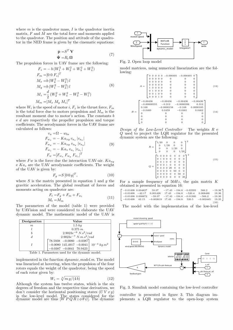
Fig. 2. Open loop model

model matrices, using numerical linearization are the fol-lowing:

A =

0 0 0 0 0 −0.000491 −0.000491 0

0 0 0 0 0 0 0 0

0 0 0 0 0 0 0 0

0 0 0 0 0 0 0 0

1 0 0 0 0 0 0 0

0 1 0 0 0 0 0 0

0 0 1 0 0 0 0 0

0 0 0 1 0 0 0 0

(13)

B =

−0.00436 −0.00436 −0.00436 −0.00436

−0.00000555 −0.312 −0.0000398 0.312

0.168 −0.0000158 −0.168 0.0000185

−0.0460 0.0459 −0.0461 0.0462

0 0 0 0

0 0 0 0

0 0 0 0

0 0 0 0

(14)

Design of the Low-Level Controller The weights R eQ used to project the LQR regulator for the presenteddynamic system are the following:

R =

[1/20 0 0 0

0 1/20 0 0

0 0 1/20 0

0 0 0 1/20

]2

Q =

1 0 0 0 0 0 0 0

0 1 0 0 0 0 0 0

0 0 1 0 0 0 0 0

0 0 0 1 0 0 0 0

0 0 0 0 20 0 0 0

0 0 0 0 0 50 0 0

0 0 0 0 0 0 50 0

0 0 0 0 0 0 0 20

2

(15)

For a sample frequency of 50Hz, the gain matrix Kobtained is presented in equation 16:[

−0.01498 0.004827 59.07 −17.43 −194.8 −0.02393 566.2 −19.36

−0.01498 −42.17 0.001426 17.43 −194.8 −520.4 0.008488 19.36

−0.01498 0.008872 −59.07 −17.43 −194.8 −0.01300 −566.2 −19.36

−0.01498 42.15 −0.002619 17.43 −194.8 520.5 −0.002445 19.35

](16)

The model with the implementation of the low-level

[0 0 0]'

wind speed (NS/EW/DU)

sqrt(m*g/(4*b))*[1 1 1 1]'

motor's hovering speed

K

feedback gain

motors' speed

WindSpeed

states

dynamic model

(0 0 0 0)

Const

W P Q R z phi theta psi

2

phi theta psi_ref

1

z_ref

selector

Fig. 3. Simulink model containing the low-level controller

controller is presented in figure 3. This diagram im-plements a LQR regulator to the open-loop system

(shown in figure 2). The simulation whose results are

0 2 4 6−1

−0.5

0

0.5

time (s)

position (m)

x

y

z

0 2 4 6−0.05

0

0.05

0.1

0.15

time(s)

angle(rad)

φ

θ

ψ

Fig. 4. Simulation to test the low-level regulator

shown in figure 4 tests the controller from [φ θ ψ z] =[0.1(rad) 0.1(rad) 0.1 (rad),−0.5(m)] to [0(rad) 0(rad)

0(rad) − 0.6(m)].

Project of the High-level Controller The high-level con-troller receives the information from image analysis andtranslate them into φ e θ references, which provides to thelow-level loop. The project of this LQR regulator is similarto the one projected before, in equation 16. The dynamicsystem found via numerical linearization is given by:[

x

y

x

y

]=

[0 0 1 0

0 0 0 1

0 0 0 0

0 0 0 0

][x

y

x

y

]+

[0 0

0 0

0 −9.81

9.81 0

][φrefθref

](17)

The Q and R weights used for the project of the controllerare shown in equation 18.

R =

(1

4 π180

[1 0

0 1

])2

Q =

[1/(0.8) 0 0 0

0 1/(0.8) 0 0

0 0 1 0

0 0 0 1

]2(18)

The regulator gain matrix obtained for the sample fre-quency of 5Hz is shown in equation 19. The block dia-gram which contains the cascade control implementationis shown in figure 5. There we can see the block diagram ofthe high-level loop. It regulates the quadrotor to a givenx y U V reference, using the projected LQR controller. Theselector blocks xy and psi are meant to select the variableswe want from the internal model. The rectifies x y blocktranslates the x y error from the inertial frame to the bodyframe.

K =

[0 0.2343 0 0.2880

−0.2343 0 −0.2880 0

](19)

The results of the the regulation from an initial position

z_refx y U V_ref

x y

x y U V

psi

Out

recti!es_x_y

psi_ref

psi

z psi_ref

phi theta_ref

xy z

phi theta psi

U V

LowLevel

K

Fig. 5. Simulink model of the high-level loop

error x = 0.2my = 0.2m are shown in figure 6. Therewe can verify that the system reaches the stable target

in approximately 2s. Once this controller validated, weconsider validated as well the cascade control proposed.

0 1 2 3 4 5−1.5

−1

−0.5

0

0.5

time(s)

position(m)

x

y

z

0 1 2 3 4 5−4

−2

0

2

4

time(s)

angle (degrees)

φ

θ

ψ

Fig. 6. Results of the high-level model simulation

3.3 Homography

Definition An homography is a geometric transforma-tion which maps entities in a projective space. It is usefulbecause it can identify the same region of an image, whena camera observes from different positions. According to[Kanatani, 1998], from the homography between two im-ages from the same planar surface, it is possible to extractthe relative position of the camera. Let pa and pb be thecoordinates of the point p in the perspectives a and b. LetHab be the homography which contains the transformationbetween both perspectives, as presented in equation 20.

pa =

[xaya1

], pb =

[xbyb1

],Hab =

[h11 h12 h13h21 h22 h23h31 h32 h33

](20)

The pb coordinates can be obtained from pa by using theequations 21 and 22:

p′b =

[w′ xbw′ ybw′

]= Habpa (21)

pb = p′b/w′ =

[xbyb1

](22)

Reconstruction of Motion We want to validate the pos-sibility of control the quadrotor dynamic model basedon homography analysis. In this part, the homography iscalculated relating two projections of points into imageplane. The implementation of such system into Simulink,is done using an s-function, which executes the shown infigure 8.

x_target

target_ x y z phi theta psi

e_xy

x y z

phi theta psi

QuadrotorSelector

sfunction_image

s-function

Fig. 7. Block diagram with homography-based closed loop.The selector block is meant to choose only x y fromthe 6DOF given by the s-function

Figure 7 shows the block diagram which makes thehomography-based control in x y. The block designed byQuadrotor, contains the model of figure 5. In the func-tional block diagram of figure 8 are shown the operationsexecuted by the s-function. The parameters to evaluate arethe following:

(1) Pixelization/resolution

Reference pose Actual pose

Points on the ground

Points on image plane

for the reference pose

Points on image plane

for the actual pose

Homography which relates both

set of points

Normal vector

A!tude of the Vehicle

Result of homography decomposi"on:

Transla"on and rota"on of the quadrotor

Fig. 8. Block diagram of the sfunction image

(2) View angle

The results shown in figure 9 are taken from a simulationbeginning in [x y z ψ] = [0.3m − 0.3m − 3m 0.2 rad] to[0m 0m − 2m 0 rad].

0 2 4 6 8 10−3

−2

−1

0

1

2

3

time(s)

angular position error(degrees)

ephi

eteta

epsi

((a)) Error to 1024 pixels, 120degrees

0 2 4 6 8 10−10

−5

0

5

10

tempo(s)

erro

de

posi

ção

angu

lar

(gra

us)

ephietetaepsi

((b)) Error to 240 pixels, 120 de-grees

Fig. 9. Angular position estimation errors for differentresolutions, using homography

Analyzing figure 9 we can verify that the estimation erroris smaller when the system stabilizes. This is justifiedbecause the reconstruction of the movement is non-linear,and it is then sensitive to the UAV attitude angles. Insteady-state we can conclude that the error decreases forbigger resolutions.

0 2 4 6 8 10−8

−6

−4

−2

0

2

4

6

time(s)

angular position error (degrees)

ephi

eteta

epsi

((a)) Error to 240 pixels, 90 de-grees

0 2 4 6 8 10−10

−5

0

5

10

tempo(s)

erro

de

posi

ção

angu

lar

(gra

us)

ephietetaepsi

((b)) Error to 240 pixels, 120 de-grees

Fig. 10. Angular position estimation errors for differentvision angles, using homography

Figure 10 shows that for the same other conditions, theaccuracy get is better if the view angle is smaller. Capturea smaller area of the image implies that the points on theground are projected onto smaller area of the image. Thegraph of figure 11 allows us to conclude that for a biggerresolution, the final control has better accuracy. To the

smaller resolution (240 pixels), a bad performance couldbe expected, but the system oscillates x y (less than 5cm),which is an acceptable result. We can thus deduce that the

1 2 3 4 5 6 7 8 9 10

−0.1

−0.05

0

0.05

0.1

time(s)

position(m)

x

y

((a)) Error to 240 pixels, 90 de-grees

1 2 3 4 5 6 7 8 9 10

−0.1

−0.05

0

0.05

0.1

time(s)

position(m)

x

y

((b)) Error to 1024 pixels, 120degrees

Fig. 11. Estimation error in x y, for different resolutionsand enlarged for the position between −0.1 and 0.1m

homography-based control is achievable, as the simulationhas shown positive results.

4. TEXTURED-IMAGE TRACKING

4.1 Tracking as a mathematic minimization problem

Once we have a controlling scheme based on homography,we need then to obtain it from the image-tracking homog-raphy. In this work, the homography is calculated fromthe parameters vector x. The goal of this image trackingalgorithm is to find the correction ∆x of x, such thats(∆x + x) coincides with the reference image, as shownin [BenHimane and Malis, 2004]. The vector ∆x can becalculated from the minimization of the quadratic error inthe vector s:

f(∆x) =1

2‖(s(∆x + x)− s(e))‖2 (23)

The solution used by [S. BenHimane, 2004] was to estimatethe Hessian matrix with a second order Taylor series of thevectorial function of s(x) over x, calculated to x = 0.The solution of the minimization problem proposed by[S. BenHimane, 2004] leads to solve eq. 24, which maybe done using the pseudo-inverse (eq. 25).

∆s ≈ −1

2(J(e) + J(xc)) ∆x (24)

∆x ≈ −(

1

2J(e) +

1

2J(xc)

)+

∆s (25)

The method is called ESM, and was validated in [S. BenHi-mane, 2004] and [BenHimanhe, 2006], however, [Tahri andMezouar, 2010] suggested to edit the way ∆x is calculated,as shown in equation 26. The difference is that he uses thesum of the pseudo-inverse of each jacobian, instead of thepseudo-inverse of the jacobians average.

∆x ≈ −(

1

2J(e)+ +

1

2J(xc)+

)∆s (26)

Some alternative ways to calculate ∆x can tried by usingthe J(x)

∣∣x=0

, reference jacobian, or by J(x), the currentjacobian, or a combination of both. For each of thecombinations, we have the following equations:

∆x ≈ −(J(e)+

)∆s (27)

∆x ≈ −(J(xc)+

)∆s (28)

Equation 29 allows to get G from x, where A(x) =∑8i=1 xiAi. The matrixes present in 30 are the base used

to represent x.

G(x) = exp(A(x)) =

∞∑i=0

1

i!A(x)

i(29)

A1 =

[0 0 1

0 0 0

0 0 0

], A2 =

[0 0 0

0 0 1

0 0 0

], A3 =

[0 1 0

0 0 0

0 0 0

], A4 =

[0 0 0

1 0 0

0 0 0

]A5 =

[1 0 0

0 −1 0

0 0 0

], A6 =

[0 0 0

0 −1 0

0 0 1

], A7 =

[0 0 0

0 0 0

1 0 0

], A8 =

[0 0 0

0 0 0

0 1 0

] (30)

4.2 Evaluation of the Algorithm in Matlab

The set of images used for testing is the sequence of imagesused by [BenHimanhe, 2006], and presented in figure 12.

Fig. 12. Sequence of images used for testing

Minimization Method To minimize the function f(∆x)we have four options, as follows:

• Algorithm ESM, equation 25• ESM version modified by Tahri, equation 26• Reference jacobian, equation 27• Current jacobian, equation 28

Pyramid of images Let an image be resized by half ntimes having now n+1 images, representing one level of thepyramid each. The use of the pyramid of images consists indoing the search level after level, from the smaller image tothe full size image, instead of searching only in the full-sizeimage. The simulation results are shown in figure 13 wherewe can verify that the minimization by current jacobianwith a 5-level pyramid minimizes the total amount oftime spent along the sequence (50s). In figure 14 we cansee the evolution of one parameter of x when we searchthe reference image in figure 11. As the current jacobianconverges faster than the other methods we choose it toproceed in the work.

Bicubic Interpolation Function The bicubic interpola-tion comes from the need to calculate the value of theimage in non-integer pixels. This can be done using severalmethods, but the bicubic interpolation was proven to be

0

10

20

30

40

50

60

70

80

1 1/2 1/4 1/8

Tim

e t

o s

ea

rch

th

e s

eq

ue

nce

(s)

Maximum scale searching

ESM

Tahri

Reference Jacobian

Current Jacobian

Fig. 13. Processing time for different minimization types,with image pyramid, to search a 152×158 pixel imagereference in a 512 × 512 image, along the sequenceshown in 12. Across the abscissa axis, we have havethe scale of the image where the program stopped tosearch, relatively to the original 512 × 512 image. Inthe bigger scale, the pyramid has 5 levels.

0 10 20 30 40 50−20

−15

−10

−5

0

Iterations number

Value of the parameters

ESM

Tahri

JI0

JI

((a)) x(1)

Fig. 14. Evolution of the first parameter of x when search-ing the reference in the image 5, after image 1

the most effective. The bicubic interpolation algorithmhas a constant, a, which varies the performance of theprogram. This part is meant to find the a value which leadsthe program to faster results. To find the a value that

Fig. 15. Interpolated point and the points used to calculatethe interpolation

−1 −0.9 −0.8 −0.7 −0.6 −0.5330

340

350

360

370

380

390

value for a

Nu

mb

er

of

ite

rati

on

Fig. 16. Number of iteration for some values of a.

gives the best performance to the program we’ve madesome tests to the sequence of images 12, varying a. Infigure 16 we can see that the best value for a is −0.74 asit minimizes the total iterations number required.

Jacobian step, ∆z A derivative is calculated by doinga difference of the image intensity in two near points,divided by the distance between both points. The jacobianstep, as we call it, is the distance between the point wherewe are measuring the derivative and the second point. Tosimplify, we call it ∆z. To find the best ∆z, the simulation

0 0.005 0.01 0.015 0.02231

232

233

234

235

236

237

ddz value (pixels)

Pro

cess

ing

tim

e (

s)o

((a)) Variation of processing timefor ∆z

0 0.005 0.01 0.015 0.02332

334

336

338

340

ddz

Ite

rati

on

s n

um

be

r

((b)) Variation in the total numberof iterations for ∆z

Fig. 17. Program performance for different values of ∆z.

was done for multiple values of the parameter, getting theplots in figure 17. We consider that the best value for ∆zis 0.006, as it have the smaller processing time and alsosmall iterations number.

Threshold coefficient Jthcoef The implementation ofthreshold consists in use only the high-gradient points todo image tracking.

330

340

350

360

370

0 0.1 0.2 0.3 0.4 0.5 0.6

Nu

mb

er o

f it

era

o

ns

Threshold

0

200

400

600

800

1000

0 0.1 0.2 0.3 0.4 0.5 0.6

Sim

ula

o

n

me

(s)

Threshold

Fig. 18. Program’s performance in function of Jthcoef

-0.015

-0.01

-0.005

0

0.005

0.01

0 0.1 0.2 0.3 0.4 0.5 0.6

Deviaon

Threshold

Parameter1

Parameter2

Parameter3

Parameter4

Parameter5

Parameter6

Fig. 19. Deviation of x for multiple values of Jthcoef,relatively to the values obtained for Jthcoef =0. Theseparameters are obtained for the searching in the image4

In figure 18 are presented the processing time and theiterations number for multiple values of Jthcoef. In figure19 are presented the variations in the 6 first parametersof vector x. There we can verify that the simulationtakes less time for bigger values of threshold and that theiterations number is minimum for thresholds between 0.2and 0.35. Analyzing figure 20 we can conclude that ψ isthe less affected by Jthcoef, keeping the error near to zero.Analyzing figures 18 and 20 we choose the value 0.3 forJthcoef, as with it the program runs faster, keeping a smalliterations number.

Maximum number of iterations The analysis of the plots(figure 21) shows that one iteration is enough to performtracking. However, three or four iterations would be moreadequate as it can guarantee more robustness for biggerdisplacements. Hereafter we will use the fixed numberof four iterations by level. When searching the wholesequence, the final displacement found was −33.75 pixelsin x −2.14 pixels in y e 2.14 degrees in z (ψ), as we cansee in figure 22.

Fig. 22. Result of image tracking along the sequence 12

4.3 Evaluation with Image Pairs

The three images from figure 23 were tested. The resultsshow that for displacements until 15 pixels and rotation of6 degrees, the algorithm can perform tracking for any ofthe tested images. For displacements above 20 pixels, onlywith the third image (figure 23) could perform tracking.Figure 24 presents one of the examples of divergence ofthe program.

((d)) Im. 1 ((e)) Im. 2 ((f)) Im. 3

Fig. 23. Images used for algorithm testing, and its mostimportant points (Jthcoef = 0.3)

Fig. 24. Example where the algorithm converges to a localminimum. In the left we can see the original imagewith the reference selected, and in the left we cansee the displaced image with the current trackingconverging to a local minimum

-0.0005

-0.0004

-0.0003

-0.0002

-0.0001

0

0.0001

0.0002

0.0003

0 0.1 0.2 0.3 0.4 0.5 0.6

Lin

ea

r d

ev

ia

on

(m

)

Threshold

x

y

z

-0.06

-0.04

-0.02

0

0.02

0.04

0.06

0 0.1 0.2 0.3 0.4 0.5 0.6

An

gu

lar

de

via

o

n (

de

gre

es)

Threshold

phi

theta

psi

((a)) Image 2 → 3, [x y z φ θ ψ] = [ 0.328 −0.440 0.996 −0.111 0.129 0.172][(3×m)(3× degrees)]

Fig. 20. Absolute error when threshold is applied, for one of the images where the search was made. The referencecoordinates are calculated without applying threshold, and are present in the caption of each sub-figure.

-0.0002

0

0.0002

0.0004

0.0006

0.0008

0 2 4 6 8 10 12

Lin

ea

r d

ev

ia

on

(m)

Maximum number of iteraons

x

y

z

-0.05

0

0.05

0.1

0.15

0 5 10 15

An

gu

lar

de

via

o

n (

de

gre

es)

Maxumum iteraons number

phi

theta

psi

Fig. 21. Results deviation in in function of the maximum allowed number of iterations.

4.4 C Implementation

Once the Matlab program is validated we proceed to Cimplementation, because of two reasons: the Matlab ver-sion is not fast enough, and because the SRV-1 requires aC written program. The C version was done in CodeBlocks[codeblocks, 2011], which uses the GNU GCC compiler andthe blackfin toolchain.

Figure 25 has a fluxogram with the layout used to developthe program in C.

Start of the Program

framecolorcvQueryFramecapture

framecvResizeframecolor

bwcvCvtColorframe

imagebuffer2structbw

makeI1pyr

image

I10

I11

I12

I13

I14

I10

I11

I12

I13

I14

pyramid

xhat

ghat

Rl0

Rl1

Rl2

Rl3

Rl4

I10

I11

I12

I13

I14

xhat

ghat

x!l

mydrawsearch

Rl0

Il0

ghattoview

todisplayImageStr2CVtoview

shows

trackingcvShowImagetodisplay

image

coli

rowi

ncols

nrows

Rl0

Rl1

Rl2

Rl3

Rl4

Rl0

Rl1

Rl2

Rl3

Rl4

makeI0pyr

framecolorcvQueryFramecapture

framecvResizeframecolor

bwcvCvtColorframe

Loop, while it

converges

Fig. 25. Fluxogram of the C program

4.5 Evaluation of the C implementation in PC

The testing results are shown in the table 2. There we cansee the program performance for each set of parameters.

((a)) Chess ((b)) Floor1 ((c)) Floor2

Fig. 26. Scenes where the program was tested

Analyzing the table, we verify that the number of levels

Window Res. N. lev.Time/frame(ms)ch. fl. 1 fl. 2

40× 64 160× 120

0 30.20 - -1 29.24 30.26 -2 31.22 28.36 -3 30.78 - -

80× 128 240× 320

1 57.18 42.33 -2 57.25 56.12 -3 68.62 56.08 -4 61.32 - -

160× 256 480× 640

1 87.58 70.18 -2 99.78 70.14 -3 108.67 82.9 -4 104.66 - -

Table 2. Performance of the C implementation into PC, where– means the program could not do image tracking

considered for the pyramid can affect the convergence ofthe program, as we can see in the floor 1 sample.

4.6 Implementation into Surveyor SRV-1

The SRV-1 belongs to UAVision, so that it is used only toimplement this program. As nobody in the company hadany touch with it before, we had to start from zero. Theinsertion of the C program in the SRV-1 board was donethrough the re-compilation of its firmware. The compilerwe used to compile the firmware, the mingw, did not have

(or had, but incomplete) some functions (as max, sqrt orprintf ), which could receive only for integers.

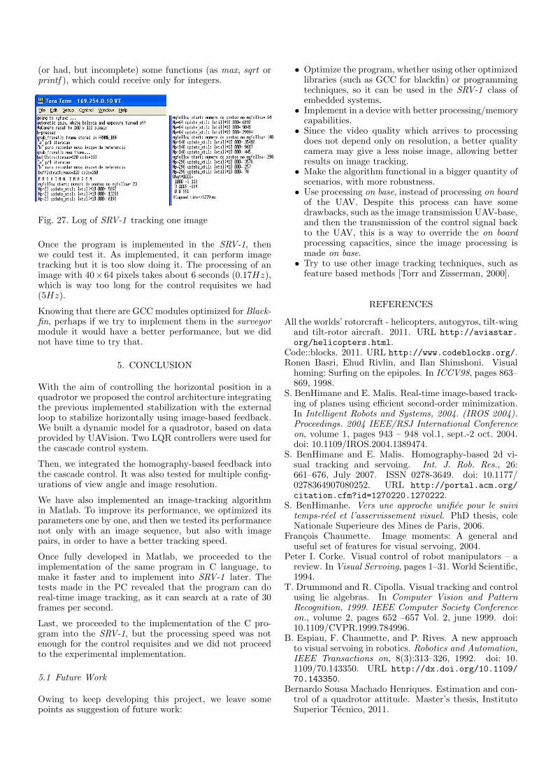
Fig. 27. Log of SRV-1 tracking one image

Once the program is implemented in the SRV-1, thenwe could test it. As implemented, it can perform imagetracking but it is too slow doing it. The processing of animage with 40×64 pixels takes about 6 seconds (0.17Hz),which is way too long for the control requisites we had(5Hz).

Knowing that there are GCC modules optimized for Black-fin, perhaps if we try to implement them in the surveyormodule it would have a better performance, but we didnot have time to try that.

5. CONCLUSION

With the aim of controlling the horizontal position in aquadrotor we proposed the control architecture integratingthe previous implemented stabilization with the externalloop to stabilize horizontally using image-based feedback.We built a dynamic model for a quadrotor, based on dataprovided by UAVision. Two LQR controllers were used forthe cascade control system.

Then, we integrated the homography-based feedback intothe cascade control. It was also tested for multiple config-urations of view angle and image resolution.

We have also implemented an image-tracking algorithmin Matlab. To improve its performance, we optimized itsparameters one by one, and then we tested its performancenot only with an image sequence, but also with imagepairs, in order to have a better tracking speed.

Once fully developed in Matlab, we proceeded to theimplementation of the same program in C language, tomake it faster and to implement into SRV-1 later. Thetests made in the PC revealed that the program can doreal-time image tracking, as it can search at a rate of 30frames per second.

Last, we proceeded to the implementation of the C pro-gram into the SRV-1, but the processing speed was notenough for the control requisites and we did not proceedto the experimental implementation.

5.1 Future Work

Owing to keep developing this project, we leave somepoints as suggestion of future work:

• Optimize the program, whether using other optimizedlibraries (such as GCC for blackfin) or programmingtechniques, so it can be used in the SRV-1 class ofembedded systems.

• Implement in a device with better processing/memorycapabilities.

• Since the video quality which arrives to processingdoes not depend only on resolution, a better qualitycamera may give a less noise image, allowing betterresults on image tracking.

• Make the algorithm functional in a bigger quantity ofscenarios, with more robustness.

• Use processing on base, instead of processing on boardof the UAV. Despite this process can have somedrawbacks, such as the image transmission UAV-base,and then the transmission of the control signal backto the UAV, this is a way to override the on boardprocessing capacities, since the image processing ismade on base.

• Try to use other image tracking techniques, such asfeature based methods [Torr and Zisserman, 2000].

REFERENCES

All the worlds’ rotorcraft - helicopters, autogyros, tilt-wingand tilt-rotor aircraft. 2011. URL http://aviastar.org/helicopters.html.

Code::blocks. 2011. URL http://www.codeblocks.org/.Ronen Basri, Ehud Rivlin, and Ilan Shimshoni. Visual

homing: Surfing on the epipoles. In ICCV98, pages 863–869, 1998.

S. BenHimane and E. Malis. Real-time image-based track-ing of planes using efficient second-order minimization.In Intelligent Robots and Systems, 2004. (IROS 2004).Proceedings. 2004 IEEE/RSJ International Conferenceon, volume 1, pages 943 – 948 vol.1, sept.-2 oct. 2004.doi: 10.1109/IROS.2004.1389474.

S. BenHimane and E. Malis. Homography-based 2d vi-sual tracking and servoing. Int. J. Rob. Res., 26:661–676, July 2007. ISSN 0278-3649. doi: 10.1177/0278364907080252. URL http://portal.acm.org/citation.cfm?id=1270220.1270222.

S. BenHimanhe. Vers une approche unifiee pour le suivitemps-reel et l’asservissement visuel. PhD thesis, coleNationale Superieure des Mines de Paris, 2006.

Francois Chaumette. Image moments: A general anduseful set of features for visual servoing, 2004.

Peter I. Corke. Visual control of robot manipulators – areview. In Visual Servoing, pages 1–31. World Scientific,1994.

T. Drummond and R. Cipolla. Visual tracking and controlusing lie algebras. In Computer Vision and PatternRecognition, 1999. IEEE Computer Society Conferenceon., volume 2, pages 652 –657 Vol. 2, june 1999. doi:10.1109/CVPR.1999.784996.

B. Espiau, F. Chaumette, and P. Rives. A new approachto visual servoing in robotics. Robotics and Automation,IEEE Transactions on, 8(3):313–326, 1992. doi: 10.1109/70.143350. URL http://dx.doi.org/10.1109/70.143350.

Bernardo Sousa Machado Henriques. Estimation and con-trol of a quadrotor attitude. Master’s thesis, InstitutoSuperior Tecnico, 2011.

Michael Isard and Andrew Blake. Contour trackingby stochastic propagation of conditional density. InBernard Buxton and Roberto Cipolla, editors, Com-puter Vision ECCV ’96, volume 1064 of Lecture Notesin Computer Science, pages 343–356. Springer Berlin /Heidelberg, 1996. URL http://dx.doi.org/10.1007/BFb0015549. 10.1007/BFb0015549.

Kenichi Kanatani. Optimal homography computationwith a reliability measure. IAPR Workshop on Ma-chine Vision Applications, Nov. 17-19. 1998, Makuhari,Chiba, Japan, 1998.

Ezio Malis and Francois Chaumette. Theoretical improve-ments in the stability analysis of a new class of model-free visual servoing methods, 2002.

Ezio Malis S. BenHimane. Real-time image-based trackingof planes using efficient second-order minimization. Pro-ceedings of the IEEE/RJS International Conference onIntelligent Robots and Systems, pages 943–948, October2004.

A.C. Sanderson and L.E. Weiss. Image-based visual servocontrol using relational graph error signals. In IEEEInternational Conference on Cybernetics and Society,page 10741077, Cambridge, Massachusetts, oct 1980.

Omar Tahri and Youcef Mezouar. On visual ser-voing based on efficient second order minimization.Robotics and Autonomous Systems, 58(5):712 – 719,2010. ISSN 0921-8890. doi: 10.1016/j.robot.2009.11.003. URL http://www.sciencedirect.com/science/article/pii/S0921889009002000.

Camillo J. Taylor and James P. Ostrowski. Robust vision-based pose control. In In International Conference onRobotics and Automation, pages 2734–2740. IEEE, 2000.

P. Torr and A. Zisserman. Feature based methods forstructure and motion estimation. In Vision Algorithms:Theory and Practice, volume 1883 of Lecture Notes inComputer Science, pages 278–294. Springer Berlin /Heidelberg, 2000. URL http://dx.doi.org/10.1007/3-540-44480-7_19.

W. J. Wilson, Williams C. C. Hulls, and G. S. Bell.Relative end-effector control using Cartesian positionbased visual servoing. 12(5):684–696, 1996.