Stabilization by oscillation - Philips Bound... · Philips tech.Rev.34,61-72,1974, No. 2/3 61 Stabilization by oscillation H. van derHeide In a corridor of the Philips Research Laboratories

Philips tech. Rev. 34,61-72,1974, No. 2/3 61

Stabilization by oscillation

H. van der Heide

In a corridor of the Philips Research Laboratories in the thirties a most unusual objectcould be seen: a pendulum balanced upside down on a pivot and held stable in this positionby a small vertical oscillation of thepivot. This little-known experiment, due to A. Stephen-son, was discovered in the literature by Balthazar van del' Pol during his analysis of'superregeneration', then a new method of radio reception. Equilibrium states analogousto that of the upside-down pendulum are to be found in widely different systems such as amarble rolling in a channel of variable contour, protons in alternating-gradient syn-chrotons and magnets levitated in combined constant and alternating magnetic fields.The feature common to all these systems is that they can be described by the Mathieudifferential equation. The question of how the parameters of such systems should bechosen to obtain stable equilibrium can be answered quite simply with the aid of a stabilitydiagram derivedfrom the Mathieu equation. The use of the diagram will be explained inthe article below by means of a few examples. A stable point must be found in the dia-gramfor each degree offreedom. Special attention is paid to levitated magnets. Themethod described here for the levitation of magnets could also be of :(nterest forfrictionless vehicles.

Introduction

According to Earnshaw's theorem it is not possibleto achieve a field configuration with permanentmagnets such that a magnet can be levitated in stableequilibrium. It may be possible to find a point wherethe total force and total couple are zero but such anequilibrium is always unstable in one or more direc-tions.

Instability in a given degree of freedom can some-times be changed to stability by an oscillation. A simpleexample is an inverted pendulum on a pivot [ll. Infig. I, M represents a mass attached to the end of a rodwhich is pivoted at the other end A. The situation infig. la is stable, that in b is unstable. The situation bcan however be stabilized by setting the point A intoforced oscillation in the vertical direction (c). A smalllateral displacement of M then no longer leads to anincreased displacement as in fig. lb but to oscillationsas in fig. la. To achieve this, the forced vertical oscil-lation of A must satisfy certain strict conditions foramplitude and frequency.A possibility that now presents itself is that the un-

stable equilibrium of a magnet levitated in a magne-

H. van der Heide is with Philips Research Laboratories, Eindhoven. [1] .See B..van der Pol, Physica 5: 157, 1925. '

rt.

A

MM

A

M.£ .

Fig. LA mass M attached to one extremity of a rigid rod which'is pivoted at the other end A, forms in (a) a pendulum in stableequilibrium and in (b) a system in unstable equilibrium. Thesituation (b) can be stabilized by oscillation of the pivot A inthe vertical direction (c).

tostatic field could perhaps be made stable in' a similar'way by means of an alternating magnetic field.This type of stability problem may be reduced:

mathematically to a certain well known differentialequation __:_the Mathieu equation ..This equ~tion. de-'scribes the behaviour ofmanywidely differing physicalsystems. The solutions of the equation are not simple:However, it is possible, without going into the solutions

, '~

62 H. VAN DER HEIDE Philips tech. Rev. 34, No. 2/3

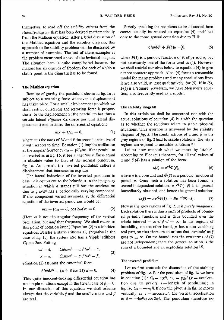
themselves, to read off the stability criteria from thestability diagram that has been derived mathematicallyfrom the Mathieu equation. After a brief discussion ofthe Mathieu equation and the stability diagram, thisapproach to the stability problem will be illustrated bya number of examples. The last of these examples isthe problem mentioned above of the levitated magnet.The situation here is quite complicated because themagnet has six degrees of freedom for each of which astable point in the diagram has to be found.

The Mathieu equation

Because of gravity the pendulum shown in fig. la issubject to a restoring force whenever a displacementhas taken place. For a small displacement (to which weshall restrict ourselves) the restoring force is propor-tional to the displacement x: the pendulum has thus acertain lateral stiffness Co (force per unit lateral dis-placement) and satisfies the differential equation:

mx + Cox = 0,

where m is the mass of M and x the second derivative ofx with respect to time. Equation (1) implies oscillationat the angular frequency Wo= VCo/m. If the pendulumis inverted as in fig. lb, it has a negative stiffness equalin absolute value to that of the normal pendulum,fig. la. As a result the inverted pendulum suffers adisplacement that increases as exp wot.

The lateral behaviour of the inverted pendulum incase le is equivalent to the behaviour in the imaginarysituation in which A stands still but the accelerationdue to gravity has a periodically varying component.If this component varied sinusoidally, the differentialequation of the inverted pendulum would be:

mx + (Co + Cl cos 2wt)x = O. (2)

(Here t» is not the angular frequency of the verticaloscillation, but halfthat frequency. We shall return tothis point of notation later.) Equation (2) is a Mathieuequation. Besides a static stiffness Co (negative in thecase of fig. le), the system also has a 'ripple' stiffnessCl cos 2wt. Putting

wt =~, Co/mw2 = W02/w2 = IX,

CI/mw2 = W12/W2= {J,x=u,equation (2) assumes the canonical form

d2u/M2 + (ct + (J cos 2~) u = O. (4)

This quite innocent-looking differential equation hasno simple solutions except in the trivial case of {J = O.In our discussion of this equation we shall assumealways that the variable ~ and the coefficients IX and (Jare real.

Strictly speaking the problems to be discussed herecannot usually be reduced to equation (4) itself butonly to the more general equation due to Hill:

(5)

where F(~) is a periodic function of ~, of period n, butnot necessarily one of the form used in (4). Howeverwe shall restrict ourselves below to equation (4) to givea more concrete approach. Also, (4) forms a reasonablemodel for many problems and many conclusions fromit are also valid, at least qualitatively, for (5). If in (5),F(~) is a 'square' waveform, we have Meissner's equa-tion, also frequently used as a model.

(1)

The stability diagram

In this article we shall be concerned not with theactual solutions of equation (4) but with the questionas to whether the solutions relate to stable physicalsituations. This question is answered by the stabilitydiagram of fig. 2. The combinations of IX and {J in thegrey regions of fig. 2 lead to stable solutions; the whiteregions correspond to unstable solutions [21.

Let us now establish what we mean by 'stable'.According to Floquet's theorem, for all real values ofIX and (J (4) has a solution of the form:

(6)

where f-l is a constant and CP(~) is a periodic function ofperiod n. Once such a solution has been found, asecond independent solution: e-Jl;CP(-~) is in generalimmediately obtained, and hence the general solution:

Now in the grey regions of fig. 2, f-l ispurely imaginary.Each solution there is thus a sum of products of bound-ed periodic functions and is thus bounded over thewhole interval - co< ~< + 00. In the regions ofinstability, on the other hand, f-l has a non-vanishingreal part, so that there are solutions that 'explode' as ~goes to ± 00. On the boundaries the two terms of (7)are not independent; there the general solution is thesum of a bounded and an exploding solution [31.

(3)

The inverted pendulum

Let us first conclude the discussion of the stabilityproblem of fig. le. For the pendulum of fig. la we havein equation (1): Co = mgll, Wo = Vifi (g = accelera-tion due to gravity, I = length of pendulum); infig.lb, Co= -mg/l. Ifnow the pivot A in fig. le movesvertically as Z - Zocos 2wt, the vertical accelerationis z = -4w2zo cos 2wt. The pendulum therefore ex-

Philips tech. Rev. 34, No. 2/3 LEVITATION

periences a vertical force corresponding to an accelera-tion g + 4w2zo cos 2wt instead of g and therefore a(lateral) stiffness of =m]l times this quantity. Inequation (2) we therefore have

Co = =mgjl,

so that (see 3):

Cl = -4mw2zo/l,

(3 = -4zo/l.

63

Parametrie excitation

To shed some light on the usual factor 2 in the arg-uments 2wt and 2ç in (2) and (4) let us consider theinverse problem for a moment: can a vertical oscil-lation of the pivot change the stable situation of fig. lainto an unstable one? From fig. 2 we can see that thisis so even for very small (infinitely small) (3, if a = 1,i.e. if w = Wo (see equation 2). The pendulum can thusbe excited into oscillation by an infinitely small vertical

Fig.2. Stability diagram for the Mathieu equation [2], on two different scales. For the corn-binations of a and f3 that lie in the grey regions, the solutions of (4) are stable, i.e. they arebounded for the whole interval - CD < ~< + CD. For combinations of a and f3 that lieoutside the grey regions there are instable solutions that 'explode' as ~ goes to ± CD. Theboundaries of the stability regions interseet the a-axis at the squares of the natural numbers.

If we now choose some value for w, then a is alsofixed. We then look at the stability diagram and finda value of (3 that gives stability for the above value ofa, and so find the amplitude Zo necessary for stability.For example, for to = Wo (a = -1), we find that 1(31must be about 3.3 to obtain stability (neglectingall stability regions except the first). This implies anamplitude of R:> 3.3 X 1/4 R:> 0.8 1. For a higher fre-quency w (smaller lal) the amplitude required issmaller.

[2] The stability diagram shown in fig. 2 and also used in otherfigures has been calculated with the aid of 'Tables relatingto Mathieu functions', National Bureau of Standards,Columbia University Press, New York 1951.

[3J More detailed information on the Mathieu equation can befound in:J. Meixner and F. W. Schäfke, Mathieusche Funktionen undSphäroidfunktionen, Springer, Berlin 1954;N. W. Mcl.achlan, Theory and application of Mathieu func-tions, Clarendon Press, Oxford 1947;E. T. Whittaker and G. N. Watson, A course of modernanalysis, 4th edition, University Press, Cambridge.See also the introduction by G. Blanch to the Tables referredto in note [2].


oscillation at a frequency exactly double the naturalfrequency of the pendulum. This is caUed parametrieexcitation [41.

Marble rolling in a channel of variable contour

Let us consider a channel whose cross-sections areparabolae of curvature varying periodically in they-direction along the channel. Let a marble roll alongthe channel at a velocity v. In the lateral directionx there is therefore a restoring force of the form-(AD + Al cos ky)x. The longitudinal distance coveredin time t is y = vt, so the equation of motion of themarble in the lateral direction is

mx + (AD + Al cos kvt)x = O.

This Mathieu equation may be put in canonical form(4) by writing:

~= ikvt,

It follows that for a given channel (AD, Al and k fixed)the ratio {3/rx is constant and equal to AI/AD; for dif-ferent velocities therefore, a straight line is describedthrough the origin in the stability diagram, towardsthe origin for increasing velocity (fig. 3). This straightline crosses alternate regions of stability and instability;this is best exemplified by the line 3. The limiting con-tours of the six channels corresponding to the sixstraight lines are shown below the stability diagram.In channel J tile motion is stable; channels between1 and 3 give broad stable regions separated by narrowunstable regions; for channels between 3 and 6, theunstable regions are broad and the stable regionsnarrow; beyond channel 6 there is no stability. Chan-nels between 5 and 6 correspond to the stability prob-lem ofthe inverted pendulum, fig. 1c; the mean stiffnessis less than zero and yet stable regions can be found.

The device shown in fig. 4 exhibits a close similarityto the marble-in-the-channel problem. It is a simplemodel to show the existence of tile stable and unstableregions. The effective stiffness of the magnet mountedon the leaf-spring varies periodically when the wheel,fitted with alternately magnetized magnets, rotates uni-formly. Jfthe wheel is first rotated rapidly (correspond-ing to a point near the origin of the stability diagram),then, as the rate of rotation diminishes, the magnet isalternately stationary and strongly oscillating.

Stabi1ization of the proton orbits in proton synchrotrons(AG focusing)

In the large circular proton accelerators built in the50s and 60s [51 a problem arises that is closely relatedto that of the marble in channel number 5 of the pre-

v Vll xx2 3 4 5 6.

Fig.3. The lateral stability of a marble rolling with velocity valong a channel of varying profile, depends on the velocity vand on the profiles. A given channel corresponds to a straightline through the origin in the stability diagram; as 'V increases,this line is traversed towards the origin. In general, then, there arestable-velocity bands alternaring with unstable bands. Below:Extreme cross-sections between which the profile of the channelvaries along its length, for six different channels correspondingto the six lines in the stability diagram. A marble in channel J isstable for all velocities; in the following channels the stableregions grow narrower and the unstable regions broader. Beyondchannel 6 there are no more stable regions.

Fig. 4. The magnet mounted on the leaf spring has a periodicallyvarying stiffness when the wheel carrying alternately magnetizedmagnets is rotated at a uniform speed. In fig. 3 the lines throughthe origin are traversed away from the origin as the velocitydecreases. Passage through an unstable region results in strongoscillations of the magnet; when the velocity corresponds to astable region the magnet becomes almost stationary. The slopeof the straight line traversed depends on the adjustment of thespring and magnet.

Philips tech. Rev. 34, No. 2/3 LEVITATION 65

VlO us problem: the focusing (beam stabilization) ofthe protons. This is usually done by means of gradientsin the 'guiding' field, i.e. the field that guides theparticles into the required circular path. An Earnshaw-type situation arises here: a field gradient that focusesin the vertical direction defocuses in the horizontaldirection, and vice versa. This may be seen as follows.For simplicity we shall disregard for a moment theguiding field and the curvature of the nominalorbit.The problem is then to hold the proton (of givenvelocity and momentum) in its (now straight) nominalpath; seefig. 5. To correct vertical deviations we needfocusing Lorentz forces F», and hence magnetic fieldsBI (assuming that the beam runs into the paper). How-ever, since the B field must be irrotational (curl B = 0),components of the type BI are always accompanied bycomponents of the type B2 and these lead to horizon-tally defocusing forces Fil.

A guiding field with a gradient, produced by meansof flared pole pieces, may be described as the super-position of a uniform guiding field and a quadrupolefield such as that of fig. 5; see fig. 6. Here we come tothe same Earnshaw-type situation. This can be easilyformulated mathematically. The horizontal deflection xand the vertical deflection z under the influence of themagnetic forces are found to satisfy the eq uations

d2x/ds2 -- (n/R2)x = 0,

d2z/ds2+ (n/R2)z = 0,

(Sa)

(Sb)

where s is the position coordinate along the nominalpath, R is the distance to the centre of the synchrotronand n is the 'field index' defined by the equalitybB/bR = -nB/R. The difference in sign between (Sa)and (Sb) expresses the difficulty: stability in x impliesinstability in z, and vice versa.

In the accelerators with weak or constant-gradient(CG) focusing this dilemma is avoided because thecentrifugal force has a weak focusing action in thehorizontal direction; this was not included in (Sa). Itcan be allowed for by replacing n in (Sa) by (n -- 1). Inthis way a positive sign is obtained in both equations ifn is taken positive but less than unity. Effectively, thereis magnetic focusing in the vertical direction but, bymaking this weak, the corresponding horizontal de-focusing remains smaller than the focusing effect of thecentrifugal force.

A revolution in the design of proton acceleratorsfollowed the discovery of the possibilities offered byMathieu's equation (or, rather, by the Hill equation).If, as in CG machines, n is a constant, then (Sa) and(Sb) can be regarded as degenerate forms of theMathieu equation, with fJ = ° and a = ± n/R2. Whenn is increased from zero, loci are traced in the stabilitydiagram (fig. 7) from 0 to A or B, i.e. into the stability

z

_--+-_8,

Ft,--~--~--------_'N~-------+----'_-x

Ft,

8,

Fig. 5. Earnshaw's theorem for a proton describing a nominallystraight path N (perpendicular to the paper). To give it a positivestiffness in the vertical direction (stabilizing forces Pv) by meansof the Lorentz force, fields of the type Bi are necessary but,because curl B = 0, these necessarily imply fields of the type B2which give a negative stiffness horizontally (defocusing forces Ph).

11111 +Fig. 6. The field of flared pole pieces (right) can be thought ofas made up of a uniform field (left) - the deflection or 'guiding'field in the case of a synchrotron - and a quadrupole field(centre) as in fig. 5. Since the guiding field contributes no stiff-ness, the proton is unstable here as in fig. 5.

Fig. 7. The nominal path of a proton passing through a series ofmagnets, all with the same field gradient (constant gradient, CG),is represented by the points A and B in the stability diagramfor displacements in the horizontal and vertical directions: in theone direction the equilibrium is stable, in the other unstable. If,however, the magnets have alternating gradients (AG), the equili-brium is stable for both directions (points Pand Q). This is thebasis of the AG focusing of proton beams.

[4] See for example B. Bollée and G. de Vries, Philips tech.Rev. 21, 47, 1959/60.

[5] See for example R. Gouiran, Philips tech. Rev. 30,330, 1969.


region with one equation and out of it with the other.When, however, n is not a constant but a sinusoidalfunction nes) of 5, a is zero and (3is not zero; and whenthe amplitude of nes) increases from zero loci aretraced in fig. 7 from 0 to P or Q, i.e. into the region ofstability for both equations.

In the CERN proton synchrotron at Geneva, whoseinstallation was completed in 1959, and in the Brook-haven alternating-gradient (AG) synchrotron in theU.S.A. completed in 1960, very effective focusing hasbeen achieved on the basis of this AG principle. Thesemachines incorporate a series of guiding magnets witha very large field index (~ 300), alternately positiveand negative. The variation in n is of course not sinus-oidal but (partly because of field-free regions in theproton path) much more complicated; however theessential thing is that n varies periodically in sign.

It is rather amusing to see the devious path by which thispossibility was discovered in 1952 at the Braakhaven labora-tory [61. Whilst the Cosmotron - the first proton synchrotron(3 GeV) - was nearing completion, studies were already underway for proton machines of higher energies. For deflection andCG focusing in the Cosmotron, C-shaped magnets were used.The useful part of the air gap in these magnets was limited bysaturation effects and it was conjectured that the useful part ofthe gaps could be made larger by placing the yoke of the magnetsalternately on the outside and the inside of the ring. The fieldgradient would then also alternate in sign and its mean wouldhave to have the required value. Calculations were made to checkthat this gradient variation would not perturb the orbit stabilitytoo much but it was found to the surprise of everyone involvedthat the stability was improved. Further calculations with strong-er alternating gradients indicated still better results and this led tothe discovery of alternating-gradient focusing (also called strongfocusing). The principle had been suggested earlier but hadattracted no attention [71.

Electrons in a periodic potential

We shall now consider the quantum-mechanicalproblem of an electron in an electric field that variesperiodically with position. A common example is ofcourse a crystal lattice, in which the periodic field isdue to the uniformly spaced ions of the lattice. Thecharge of all the other electrons may be thought of assmoothed out to a homogeneous continuous charge.This problem is usually attacked not by means of theMathieu equation but with the Hill or Meissnerequations; qualitatively, however, the results are thesame. We shall restrict the problem to one dimen-sion. The Schrödinger equation for the wave function1jJ(x) of the electron is then

d21jJ/dx2 + 8n2mh-2 {E- V(x)}1jJ = O. (9)

E is the total energy and m the mass of the electron,Vex) is its potential energy as a result of the electric

field, and h is Planck's constant. We write:

Vex) = Vo - VI cos (2nx/a),

where a, the lattice parameter, is the spatial period ofthe electric field. To reduce (9) to the canonical form(4) we must put:

ç = stxl a, a = 8mh-2a2(E - Vo), (3= 8mh-2a2 Vl.

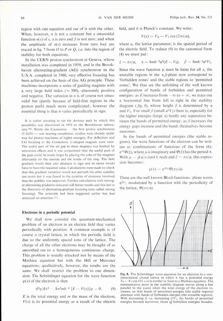
Since the wave function 1jJmust be finite for all x, theunstable regions in the a,(3-plane now correspond to'forbidden zones' and the stable regions to 'permittedzones'. We thus see the unfolding of the well knownconfiguration of bands of forbidden and permittedenergies: as E increases from -00 to + 00, we trace outa horizontal line from left to right in the stabilitydiagram (fig. 8), whose height (3 is determined by aand VI. For small (3(small a2V1) there is, especially forthe higher energies (large a) hardly any separation be-tween the bands of permitted energy; as (3increases theenergy gaps increase and the bands themselves becomenarrower.

In the bands of permitted energies (the stable re-gions), the wave functions of the electron can be writ-ten as combinations of functions of the form (6):eI'~W(ç),where fl is imaginary and W(ç) has the period re.With fl = jka/n (and le real) and ç = nx]a, this expres-sion becomes:

1fJ(x) = ejkxW(nx/a).

These are the well known Bloch functions: plane wavesejkX, modulated by a function with the periodicity ofthe lattice, W(nx/a).

-aFig. 8. The Schrödinger wave equation for an electron in a one-dimensional crystal lattice in which it has a potential energyVo - VI cos (2n x/a) is similar in form to a Mathieu equation. Therepresentative point in the stability diagram moves along a lineparallel to the a-axis when the total energy of the electron in-creases, so that bands of permitted energies (the stable regions)alternate with bands of forbidden energies (the unstable regions).With increasing fJ, i.e. increasing a2 VI, the bands of permittedenergies become narrower, those ol forbidden energies broader.


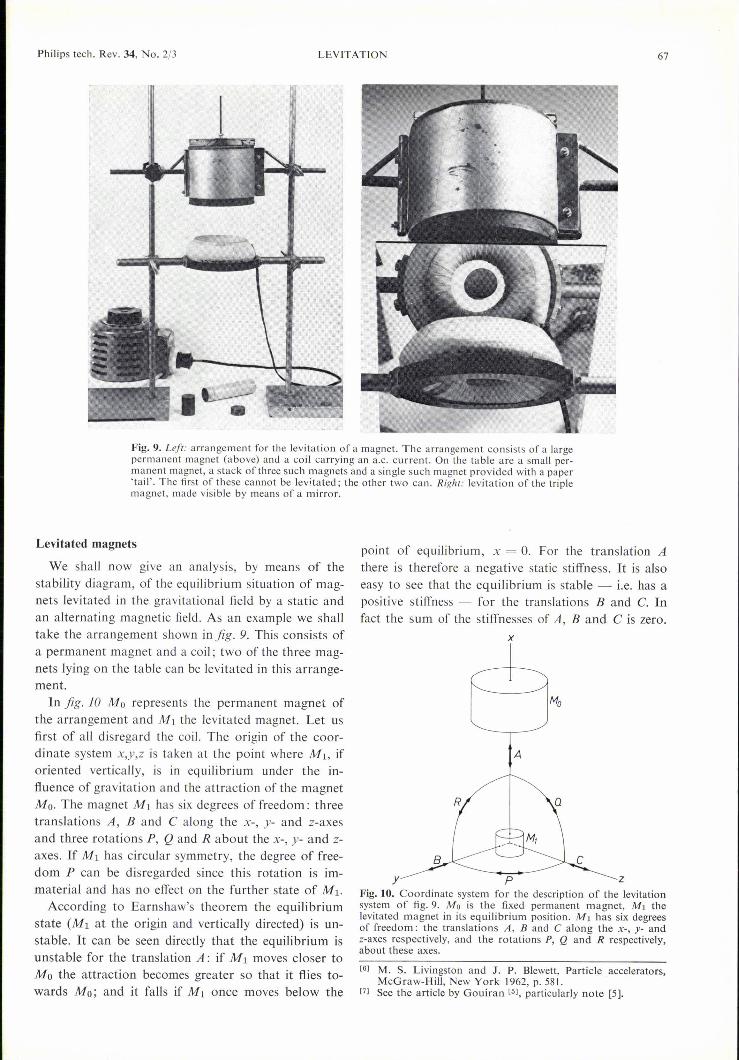
Fig. 9. Left: arrangement for the levitation of a magnet. The arrangement consists of a largepermanent magnet (above) and a coil carrying an a.C. current. On the table are a small per-manent magnet, a stack of three such magnets and a single such magnet provided with a paper'tail'. The first of these cannot be levitated; the other two can. Right: levitation of the triplemagnet, made visible by means of a mirror.

Levitated magnets

We shall now give an analysis, by means of thestability diagram, of the equilibrium situation of mag-nets levitated in the gravitational field by a static andan alternating magnetic field. As an example we shalltake the arrangement shown in fig. 9. This consists ofa permanent magnet and a coil; two of the three mag-nets lying on the table can be levitated in this arrange-ment.

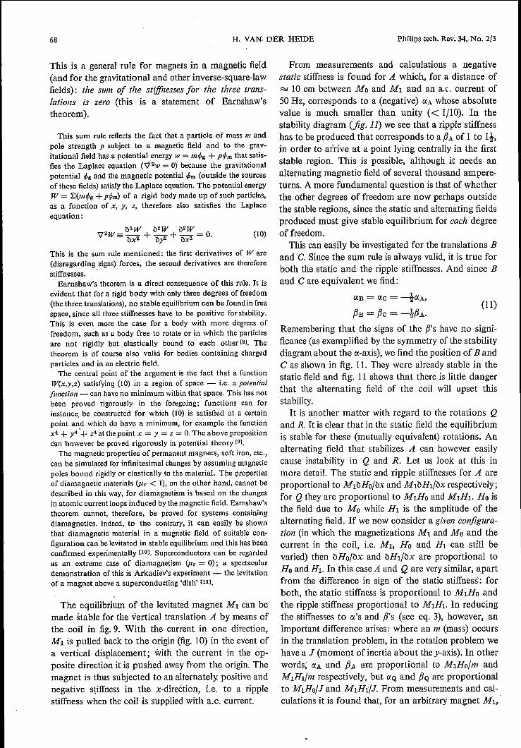
ln fig. 10 M« represents the permanent magnet ofthe arrangement and MI the levitated magnet. Let usfirst of all disregard the coil. The origin of the coor-dinate system x,y,z is taken at the point where MI, iforiented vertically, is in equilibrium under the in-fluence of gravitation and the attraction of the magnetM«. The magnet MI has six degrees of freedom: threetranslations A, Band C along the x-, y- and z-axesand three rotations P, Q and R about the x-, y- and z-axes. If MI has circular symmetry, the degree of free-dom P can be disregarded since this rotation is im-material and has no effect on the further state of MI.

According to Earnshaw's theorem the equilibriumstate (MI at the origin and vertically directed) is un-stable. It can be seen directly that the equilibrium isunstable for the translation A: if MI moves closer toMo the attraction becomes greater so that it flies to-wards M«; and it falls if MI once moves below the

point of equilibrium, x = O. For the translation Athere is therefore a negative static stiffness. It is alsoeasy to see that the equilibrium is stable - i.e. has apositive stiffness - for the translations Band C. Infact the sum of the stiffnesses of A, Band C is zero.

x

A

y zFig. 10. Coordinate system for the description of the levitationsystem of fig. 9. M« is the fixed permanent magnet, MI thelevitated magnet in its equilibrium position. MI has six degreesof freedom: the translations A, Band C along the X-, y- andz-axes respectively, and the rotations P, Q and R respectively,about these axes.

[6J M. S. Livingston and J. P. Blewett, Particle accelerators,McGraw-Hill, New York 1962, p. 581.

[7J See the article by Gouiran [5J, particularly note [5].

68 H. VAN DER HEIDE Philips tech. Rev. 34,.No. 2/3

This is a general rule for magnets in a magnetic field(and for the gravitational and other inverse-square-lawfields): the sum of the stiffnesses for the three trans-lations is zero (this is a statement of Earnshaw'stheorem).

This sum rule reflects the fact that a particle of mass /11 andpole strength p subject to a magnetic field and to the grav-itational field has a potential energy JV = mrPg + PrPm that satis-fies the Laplace equation (V'2JV = 0) because the gravitationalpotential rPg and the magnetic potential rpm(outside the sourcesof these fields) satisfy the Laplace equation. The potential energyW = '2:.(mrPg + prpm) of a rigid body made up of such particles,as a function of x, y, z, therefore also satisfies the Laplaceequation:

This is the sum rule mentioned: the first derivatives of Ware(disregarding signs) forces, the second derivatives are thereforestiffnesses. .

Earnshaw's theorem is a direct consequence of this rule. It isevident that for a rigid body with only three degrees of freedom(the three translations), no stable equilibrium can be found in freespace, since all three stiffnesses have to be positive for stability.This is even more the case for a body with more degrees offreedom, such as a body free to rotate or in which the particlesare not rigidly but elastically bound to each other [8J. Thetheorem is of course also valid for bodies containing chargedparticles and in an electric field.The central point of the argument is the fact that a function

W(x,y,z) satisfying (10) in a region of space - i.e. a potentialfunction - can have no minimum within that space. This has notbeen proved rigorously in the foregoing; functions can forinstance. be constructed for which (10) is satisfied at a certainpoint and which do have a minimum, for example the functionx4 + y4 '+ z4 at the point x = y = z = O.The above propositioncan however be proved rigorously in potential theory [9J.

The magnetic properties of permanent magnets, soft iron, etc.,can be simulated for infinitesimal changes by assuming magneticpoles bound rigidly or elastically to the material. The propertiesof diamagnetic materials (pr < 1), on the other hand, cannot bedescribed in this way, for diamagnetism is based on the changesin atomic current loops induced by the magnetic field. Earnshaw'stheorem cannot, therefore, be proved for systems containingdiamagnetics. Indeed, to the contrary, it can easily be shownthat diamagnetic material in a magnetic field of suitable con-figuration can be levitated in stable equilibrium and this has beenconfirmed experimentally [10J. Superconductors can be regardedas an extreme case of diamagnetism (pr = 0); a spectaculardemonstration of this is Arkadiev's experiment - the levitationof a magnet above a superconducting 'dish' [111.

The equilibrium of the levitated magnet MI can bemade stable for the vertical translation A by means ofthe coil in fig.9. With the current in one direction,MI is pulled back to the origin (fig. 10) in the event ofa vertical displacement; with the current in the op-posite direction it is pushed away from the origin. Themagnet is thus subjected to an alternately. positive andnegative stiffness in the x-direétion, i.e. to a ripplestiffness when the coil is supplied with a.c. current.

(10)

From measurements and calculations a negativestatic stiffness is found for A which, for a distance ofRi 10 cm between Mo and MI and an a.c. current of50 Hz, corresponds to a (negative) ('/,A whose absolutevalue is much smaller than unity « 1/10). In thestability diagram (fig. 11) we see that a ripple stiffnesshas to be produced that corresponds to a {h of 1 to It,in order to arrive at a point lying centrally in the firststable region. This is possible, although it needs analternating magnetic field of several thousand ampere-turns. A more fundamental question is that of whetherthe other degrees of freedom are now perhaps outsidethe stable regions, since the static and alternating fieldsproduced must give stable equilibrium for each degreeof freedom.This can easily be investigated for the translations B

and C. Since the sum rule is always valid, it is true forboth the static and the ripple stiffnesses. And since Band C are equivalent we find:

('/,B = ('/,e = --i('/,A,(11)

{JB = {Je = --i{JA.Remembering that the signs of the {J's have no signi-ficance (as exemplified by the symmetry of the stabilitydiagram about the «-axis), we find the position of BandC as shown in fig. 11. They were already stable in thestatic field and fig. 11 shows that there is little dangerthat the alternating field of the coil will upset thisstability.It is another matter with regard to the rotations Q

and R. It is clear that in the static field the equilibriumis stable for these (mutually equivalent) rotations. Analternating field that stabilizes A can however easilycause instability in Q and R. Let us look at this inmore detail. The static and ripple stiffnesses for A areproportional to MIOHo/bx and MIOHI/bx respectively;for Q they are proportional to MIHo and MIHI. Ho isthe field due to Mo while HI is the amplitude of thealternating field. If we now consider a given configura-tion (in which the magnetizations MI and Mo and thecurrent in the coil, i.e. M!, Ho and HI can still bevaried) then oH%x and OHI/OX are proportional toHo and HI. In this case A and Q are very similar, apartfrom the difference in sign of the static stiffness': forboth, the static stiffness is proportional to MIHo andthe ripple stiffness proportional to MIHI. In reducingthe stiffnesses to ('/,'sand {J's (see eq. 3), however, animportant difference arises: where an m (mass) occursinthe translation problem, in the rotation problem wehave a J (moment of inertia about the y-axis). In otherwords; ('/,A and {JA are proportional to MIHo/m andMIHI/m respectively, but ('/,Q and {JQ are proportionalto MIHo/J and MIHl/J. From measurements and cal-culations it is found that, for an arbitrary magnet MI,


-1

Fig. 11. The equilibrium for the translations A, Band C and therotation Q represented in the stability diagram for a magnet witha relatively small moment of inertia J in the arrangement offig. 9. It is assumed that IIXAI« I, and that the equilibrium forthe translation A is stabilized by means of the alternating field ofthe coil. The positions of Band C in the diagram then followfrom eq. (11); in general they are found to lie in the stable region.The distance of the point Q from the origin is inversely pro-portional to J. For a relatively small J, Q lies in an unstableregion. If J is increased (without changing MI/In), Q movestowards the origin (while A, Band C remain where they are) sothat stable levitation may become possible.

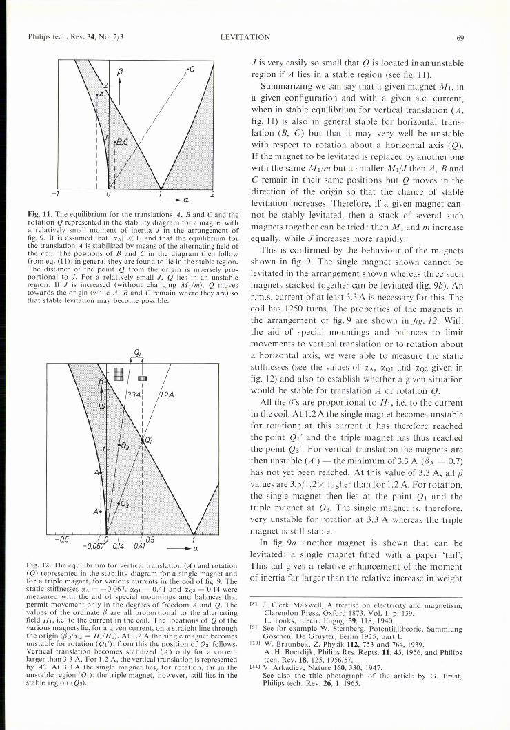
Fig. 12. The equilibrium for vertical translation (A) and rotation(Q) represented in the stability diagram for a single magnet andfor a triple magnet, for various currents in the coilof fig. 9. Thestatic stiffnesses (XA = -0.067, IXQl= 0.41 and (XQ3 = 0.14 weremeasured with the aid of special mountings and balances thatpermit movement only in the degrees of freedom A and Q. Thevalues of the ordinate f3 are all proportional to the alternatingfield HI, i.e. to the current in the coil. The locations of Q of thevarious magnets lie, for a given current, on a straight line throughthe origin (f3Q/(XQ = Hl/ Ho). At 1.2 A the single magnet becomesunstable for rotation (Ql'); from this the position of Q3' follows.Vertical translation becomes stabilized (A) only for a currentlarger than 3.3 A. For 1.2 A, the vertical translation is representedby A'. At 3.3 A the single magnet lies, for rotation, far in theunstable region (Ql); the triple magnet, however, still lies in thestable region (Q3).

J is very easily so small that Q is located in an unstableregion if A lies in a stable region (see fig. 11).

Summarizing we can say that a given magnet MI, ina given configuration and with a given a.c. current,when in stable equilibrium for vertical translation (A,fig. 11) is also in general stable for horizontal trans-lation (B, C) but that it may very well be unstablewith respect to rotation about a horizontal axis (Q).If the magnet to be levitated is replaced by another onewith the same Ml/m but a smaller MIl] then A, BandC remain in their same positions but Q moves in thedirection of the origin so that the chance of stablelevitation increases. Therefore, if a given magnet can-not be stably levitated, then a stack of several suchmagnets together can be tried: then MI and m increaseequally, while] increases more rapidly.

This is confirmed by the behaviour of the magnetsshown in fig. 9. The single magnet shown cannot belevitated in the arrangement shown whereas three suchmagnets stacked together can be levitated (fig. 9b). Anr.m.s. current of at least 3.3 A is necessary for this. Thecoil has 1250 turns. The properties of the magnets inthe arrangement of fig. 9 are shown in fig. 12. Withthe aid of special mountings and balances to limitmovements to vertical translation or to rotation abouta horizontal axis, we were able to measure the staticstiffnesses (see the values of (Y.A, (Y.QI and (Y.Q3 given infig. 12) and also to establish whether a given situationwould be stable for translation A or rotation Q.

All the (3's are proportional to HI, i.e. to the currentin the coil. At 1.2 A the single magnet becomes unstablefor rotation; at this current it has therefore reachedthe point QI' and the triple magnet has thus reachedthe point Q3'. For vertical translation the magnets arethen unstable (A') - the minimum of 3.3 A ((3A = 0.7)has not yet been reached. At this value of 3.3 A, all (3values are 3.3/1.2 X higher than for 1.2 A. For rotation,the single magnet then lies at the point QI and thetriple magnet at Q3. The single magnet is, therefore,very unstable for rotation at 3.3 A whereas the triplemagnet is still stable.

ln fig. 9a another magnet is shown that can belevitated: a single magnet fitted with a paper 'tail'.This tail gives a relative enhancement of the momentof inertia far larger than the relative increase in weight

[8] J. Clerk Maxwell, A treatise on electricity and magnetism,ClarencIon Press, Oxford 1873, Vol. I, p. 139.L. Tanks, Electr. Engng. 59, 1 18, 1940.

[9] See for example W. Sternberg, Potentialtheorie, SammlungGöschen, De Gruyter, Berlin 1925, part l.

[10] W. Braunbek, Z. Physik 112, 753 and 764, 1939.A. H. Boerdijk, Philips Res. Repts. 11,45, 1956, and Philipstech. Rev. 18, 125, 1956/57.

[11] V. Arkacliev, Nature 160, 330, 1947.See also the title photograph of the article by G. Prast,Philips tech. Rev. 26, I, 1965.


so that the position of A in the diagram (fig. 12) is littleaffected whereas Ql is moved considerably in the direc-tion of the origin.

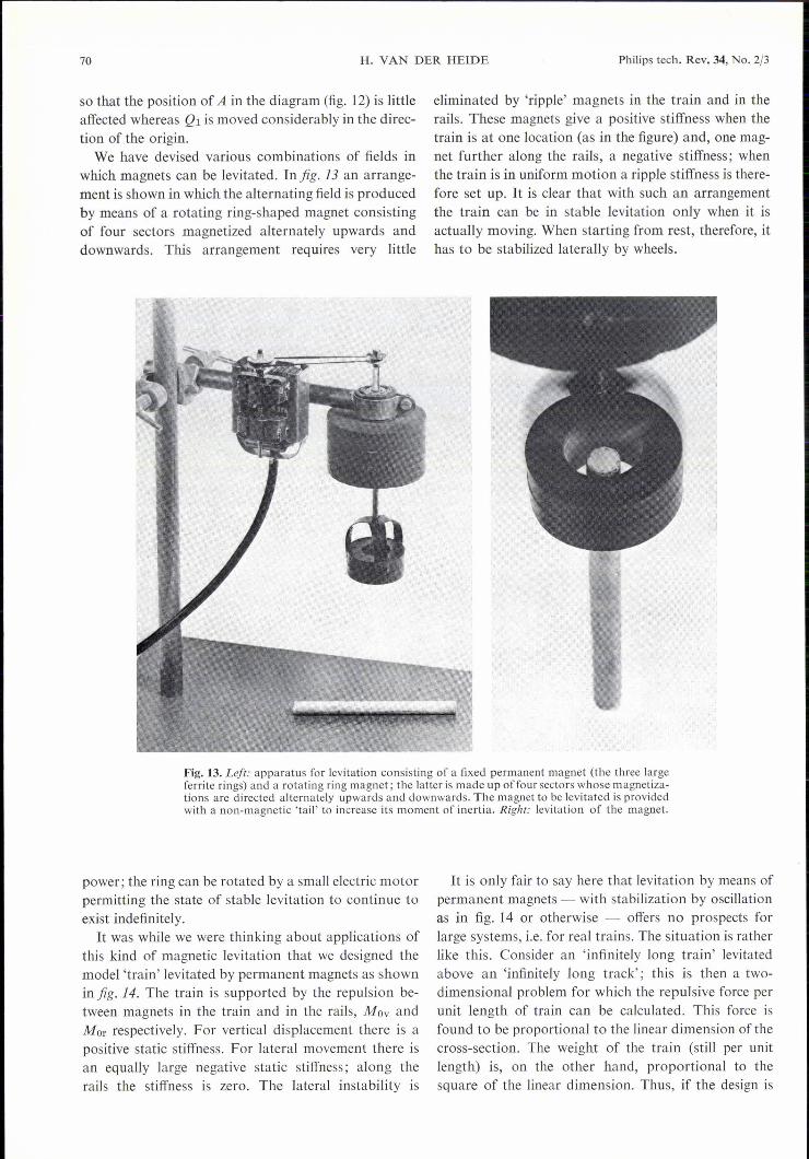
We have devised various combinations of fields inwhich magnets can be levitated. In fig. 13 an arrange-ment is shown in which the alternating field is producedby means of a rotating ring-shaped magnet consistingof four sectors magnetized alternately upwards anddownwards. This arrangement requires very little

eliminated by 'ripple' magnets in the train and in therails. These magnets give a positive stiffness when thetrain is at one location (as in the figure) and, one mag-net further along the rails, a negative stiffness; whenthe train is in uniform motion a ripple stiffness is there-fore set up. It is clear that with such an arrangementthe train can be in stable levitation only when it isactually moving. When starting from rest, therefore, ithas to be stabilized laterally by wheels.

Fig. 13. Left: apparatus for levitation consisting of a fixed permanent magnet (the three largeferrite rings) and a rotating ring magnet; the latter is made up offour sectors whose magnetiza-tions are directed alternately upwards and downwards. The magnet to be levitated is providedwith a non-magnetic 'tail' to increase its moment of inertia. Right: levitation of the magnet.

power; the ring can be rotated by a small electric motorpermitting the state of stable levitation to continue toexist indefinitely.It was while we were thinking about applications of

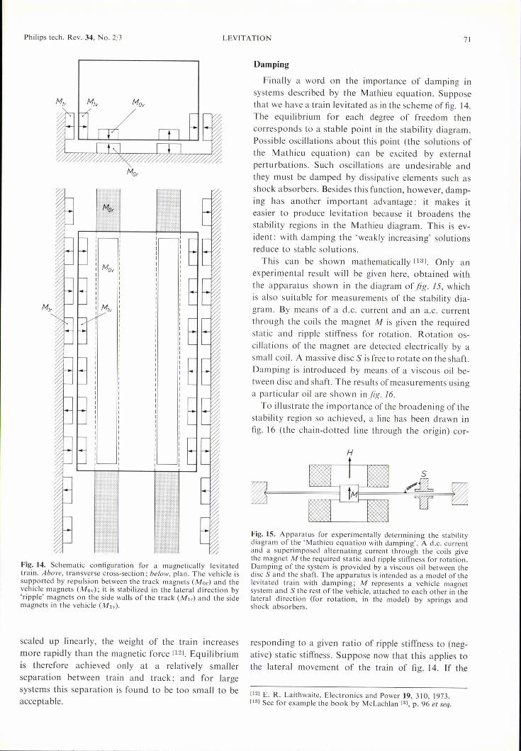
this kind of magnetic levitation that we designed themodel 'train' levitated by permanent magnets as shownin fig. 14. The train is supported by the repulsion be-tween magnets in the train and in the rails, Mov andMor respectively. For vertical displacement there is apositive static stiffness. For lateral movement there isan equally large negative static stiffness; along therails the stiffness is zero. The lateral instability is

It is only fair to say here that levitation by means ofpermanent magnets - with stabilization by oscillationas in fig. 14 or otherwise - offers no prospects forlarge systems, i.e. for real trains. The situation is ratherlike this. Consider an 'infinitely long train' levitatedabove an 'infinitely long track'; this is then a two-dimensional problem for which the repulsive force perunit length of train can be calculated. This force isfound to be proportional to the linear dimension of thecross-section. The weight of the train (still per unitlength) is, on the other hand, proportional to thesquare of the linear dimension. Thus, if the design is

Philips tech. Rev. 34, No. 2/3

Fig. 14. Schematic configuration for a magnetically levitatedtrain. Above, transverse cross-section ; below, plan. The vehicle issupported by repulsion between the track magnets (Mo,.) and thevehicle magnets (Mov); it is stabilized in the lateral direction by'ripple' magnets on the side walls of the track (Mlr) and the sidemagnets in the vehicle (Mlv).

scaled up linearly, the weight of the train increasesmore rapidly than the magnetic force [12]. Equilibriumis therefore achieved only at a relatively smallerseparation between train and track; and for largesystems this separation is found to be too small to beacceptable.

LEVITATION 71

Damping

Finally a word on the importance of damping insystems described by the Mathieu equation. Supposethat we have a train levitated as in the scheme offig. 14.The equilibrium for each degree of freedom thencorresponds to a stable point in the stability diagram.Possible oscillations about this point (the solutions ofthe Mathieu equation) can be excited by externalperturbations. Such oscillations are undesirable andthey must be damped by dissipative elements such asshock absorbers. Besides this function, however, damp-ing has another important advantage: it makes iteasier to produce levitation because it broadens thestability regions in the Mathieu diagram. This is ev-ident: with damping the 'weakly increasing' solutionsreduce to stable sol utions.

This can be shown mathematically [13]. Only anexperimental result will be given here, obtained withthe apparatus shown in the diagram of jig. 15, whichis also suitable for measurements of the stability dia-gram. By means of a d.c. current and an a.c. currentthrough the coils the magnet M is given the requiredstatic and ripple stiffness for rotation. Rotation os-cillations of the magnet are detected electrically by asmall coil. A massive disc S is free to rotate on the shaft.Damping is introduced by means of a viscous oil be-tween disc and shaft. The results ofmeasurements usinga particular oil are shown in fig. 16.

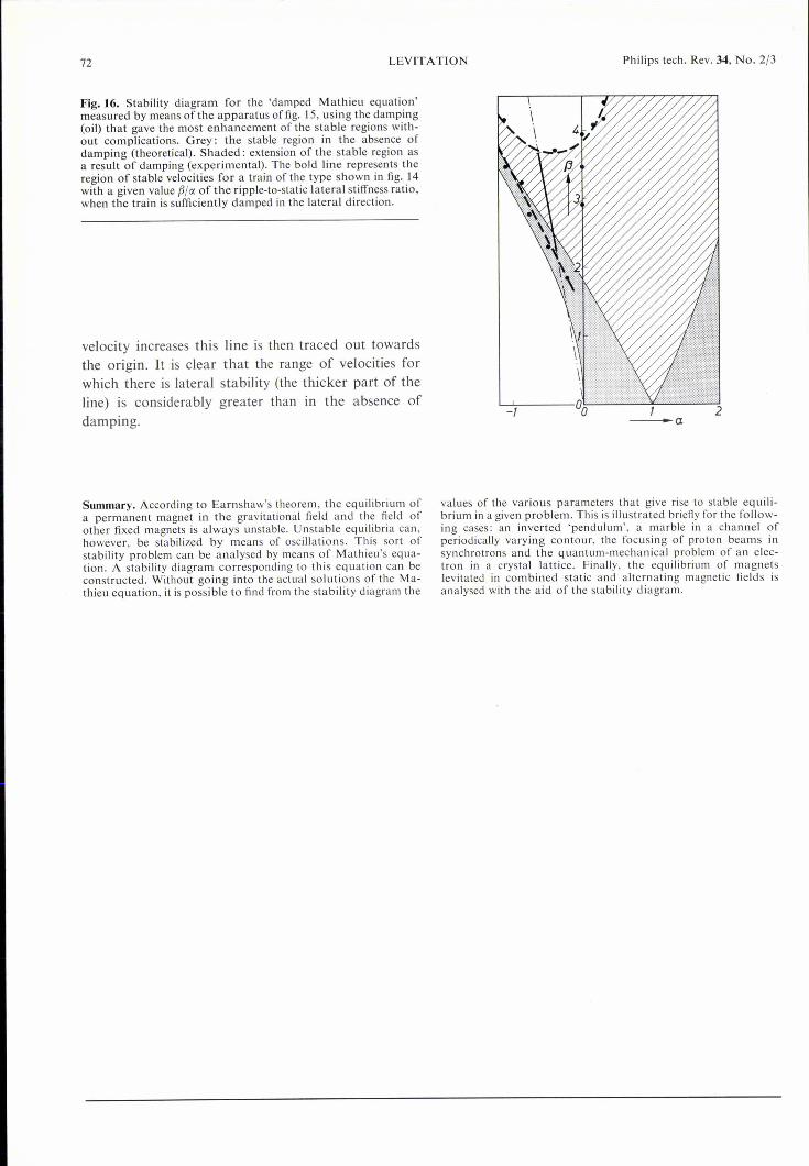
To illustrate the importance ofthe broadening ofthestability region so achieved, a line has been drawn infig. 16 (the chain-dotted line through the origin) cor-

H

Fig. IS. Apparatus for experimentally determining the stabilitydiagram of the 'Mathieu equation with damping'. A d.c. currentand a superimposed alternating current through the coils givethe magnet M the required static and ripple stiffness for rotation.Damping of the system is provided by a viscous oil between thedisc S and the shaft. The apparatus is intended as a model of thelevitated train with damping; M represents a vehicle magnetsystem and S the rest of the vehicle, attached to each other in thelateral direction (for rotation, in the model) by springs andshock absorbers.

responding to a given ratio of ripple stiffness to (neg-ative) static stiffness. Suppose now that this applies tothe lateral movement of the train of fig. 14. If the

(12] E. R. Laithwaite, Electronics and Power 19,310,1973.(13] See for example the book by McLachlan (3], p. 96 et seq.

72 LEVITATION Philips tech. Rev. 34, No. 2/3

Fig.16. Stability diagram for the 'damped Mathieu equation'measured by means of the apparatus offig. 15, using the damping(oil) that gave the most enhancement of the stable regions with-out complications. Grey: the stable region in the absence ofdamping (theoretical). Shaded: extension of the stable region asa result of damping (experimental). The bold line represents theregion of stable velocities for a train of the type shown in fig. 14with a given value B]« of the ripple-to-static lateral stiffness ratio,when the train is sufficiently damped in the lateral direction.

velocity increases this line is then traced out towardsthe origin. It is clear that the range of velocities forwhich there is lateral stability (the thicker part of theline) is considerably greater than in the absence ofdamping.

Summary. According to Earnshaw's theorem, the equilibrium ofa permanent magnet in the gravitational field and the field ofother fixed magnets is always unstable. Unstable equilibria can,however, be stabilized by means of oscillations. This sort ofstability problem can be analysed by means of Matbieu's equa-tion. A stability diagram corresponding to this equation can beconstructed. Without going into the actual solutions of the Ma-thieu equation, it is possible to find from the stability diagram the

-a

values of the various parameters that give rise to stable equili-brium in a given problem. This is illustrated briefly for the follow-ing cases: an inverted 'pendulum', a marble in a channel ofperiodically varying contour, the focusing of proton beams insynchrotrons and the quantum-mechanical problem of an elec-tron in a crystal lattice. Finally, the equilibrium of magnetslevitated in combined static and alternating magnetic fields isanalysed with the aid of the stability diagram.

Documents

Stabilization by oscillation - Philips Bound... · Philips tech.Rev.34,61-72,1974, No. 2/3 61 Stabilization by oscillation H. van derHeide In a corridor of the Philips Research Laboratories