Stability of Grazing Systems: An Application of Predator-Prey Graphs · 2013-11-11 · STABILITY OF GRAZING SYSTEMS: AN APPLICATION OF PREDATOR-PREY GRAPHS ... Some explicit forms

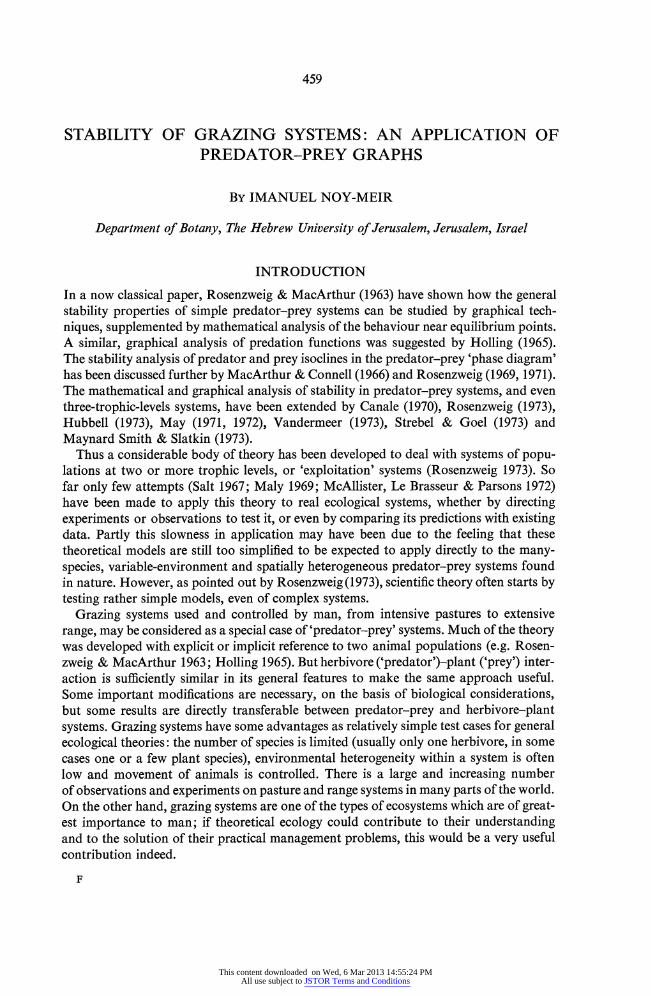
459

STABILITY OF GRAZING SYSTEMS: AN APPLICATION OF PREDATOR-PREY GRAPHS

BY IMANUEL NOY-MEIR

Department of Botany, The Hebrew University of Jerusalem, Jerusalem, Israel

INTRODUCTION

In a now classical paper, Rosenzweig & MacArthur (1963) have shown how the general stability properties of simple predator-prey systems can be studied by graphical techniques, supplemented by mathematical analysis of the behaviour near equilibrium points. A similar, graphical analysis of predation functions was suggested by Holling (1965). The stability analysis of predator and prey isoclines in the predator-prey 'phase diagram' has been discussed further by MacArthur & Connell (1966) and Rosenzweig (1969, 1971). The mathematical and graphical analysis of stability in predator-prey systems, and even three-trophic-levels systems, have been extended by Canale (1970), Rosenzweig (1973), Hubbell (1973), May (1971, 1972), Vandermeer (1973), Strebel & Goel (1973) and Maynard Smith & Slatkin (1973).

Thus a considerable body of theory has been developed to deal with systems of populations at two or more trophic levels, or 'exploitation' systems (Rosenzweig 1973). So far only few attempts (Salt 1967; Maly 1969; McAllister, Le Brasseur & Parsons 1972) have been made to apply this theory to real ecological systems, whether by directing experiments or observations to test it, or even by comparing its predictions with existing data. Partly this slowness in application may have been due to the feeling that these theoretical models are still too simplified to be expected to apply directly to the many- species, variable-environment and spatially heterogeneous predator-prey systems found in nature. However, as pointed out by Rosenzweig (1973), scientific theory often starts by testing rather simple models, even of complex systems.

Grazing systems used and controlled by man, from intensive pastures to extensive

range, may be considered as a special case of'predator-prey' systems. Much of the theory was developed with explicit or implicit reference to two animal populations (e.g. Rosen-

zweig & MacArthur 1963; Holling 1965). But herbivore ('predator')-plant ('prey') interaction is sufficiently similar in its general features to make the same approach useful. Some important modifications are necessary, on the basis of biological considerations, but some results are directly transferable between predator-prey and herbivore-plant systems. Grazing systems have some advantages as relatively simple test cases for general ecological theories: the number of species is limited (usually only one herbivore, in some cases one or a few plant species), environmental heterogeneity within a system is often low and movement of animals is controlled. There is a large and increasing number of observations and experiments on pasture and range systems in many parts of the world. On the other hand, grazing systems are one of the types of ecosystems which are of great- est importance to man; if theoretical ecology could contribute to their understanding and to the solution of their practical management problems, this would be a very useful contribution indeed.

F

This content downloaded on Wed, 6 Mar 2013 14:55:24 PMAll use subject to JSTOR Terms and Conditions

http://www.jstor.org/page/info/about/policies/terms.jsp

460 Stability of grazing systems

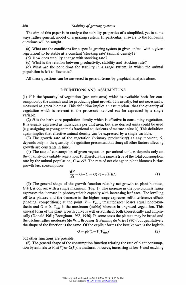
The aim of this paper is to analyse the stability properties of a simplified, yet in some ways rather general, model of a grazing system. In particular, answers to the following questions will be sought.

(a) What are the conditions for a specific grazing system (a given animal with a given vegetation) to be stable at a constant 'stocking rate' (animal density)?

(b) How does stability change with stocking rate ? (c) What is the relation between productivity, stability and stocking rate? (d) What are the conditions for stability in a range system, in which the animal

population is left to fluctuate ?

All these questions can be answered in general terms by graphical analysis alone.

DEFINITIONS AND ASSUMPTIONS

(1) V is the 'quantity' of vegetation (per unit area) which is available both for consumption by the animals and for producing plant growth. It is usually, but not necessarily, measured as green biomass. This definition implies an assumption: that the quantity of vegetation which is relevant to the processes involved can be expressed by a single variable.

(2) H is the herbivore population density which is effective in consuming vegetation. It is usually expressed as individuals per unit area, but also derived units could be used (e.g. assigning to young animals fractional equivalents of mature animals). This definition again implies that effective animal density can be expressed by a single variable.

(3) The growth rate of the vegetation (primary productivity) at any moment, G, depends only on the quantity of vegetation present at that time; all other factors affecting growth are constants in time.

(4) The rate of consumption of green vegetation per animal unit, c, depends only on the quantity of available vegetation, V. Therefore the same is true of the total consumption rate by the animal population, C = cH. The rate of net change in plant biomass is thus growth less consumption

dV d G - C = G(V)-c(V)H. (1) at

(5) The general shape of the growth function relating net growth to plant biomass, G(V), is convex with a single maximum (Fig. 1). The increase in the low-biomass range expresses the increase in photosynthetic capacity with increasing leaf area. The levelling off to a plateau and the decrease in the higher range expresses self-interference effects (shading, competition); at the point V = Vma,, 'maintenance' losses equal photosyn- thesis and G = 0. Vmax is the maximum (stable) biomass in ungrazed vegetation. This general form of the plant growth curve is well established, both theoretically and empiri- cally (Donald 1961; Brougham 1955, 1956). In some cases the plateau may be broad and the decline rather moderate (de Wit, Brouwer & Penning de Vries 1970), but qualitatively the shape of the function is the same. Of the explicit forms the best known is the logistic

G = gV(1- V/Vmax) (2)

but other functions are possible. (6) The general shape of the consumption function relating the rate of plant consump-

tion by animals to V, c(V) or C(V), is a saturation curve, increasing at low Vand reaching



IMANUEL NOY-MEIR 461

Fig. I Fig. 2

G C

/// \ \\/ /

4 1/ Vm l

FIG. 1. Plant growth (G) as function of plant biomass (V). (a) Logistic growth; G,- maximal growth, Vx-biomass at which growth is maximal. (b) and (c) Other possible curves.

FIG. 2. Consumption per animal (c) as function of plant biomass. cm-Maximal consumption. (a) Linear to satiation. (b) Gradual satiation curve (e.g. Michaelis). (c) Sigmoid.

a plateau at high V (Fig. 2). At low V, intake is limited by forage availability and increases with it while, at high V, a saturation of intake capacity (digestion rate) is reached. Various types of such functions ('ramp', smoothly convex, sigmoid) have been found experimentally for predators (Holling 1965, 1966) and for herbivores (Willoughby 1959; Allden 1962; Ivlev 1961). Some explicit forms are the Michaelis equation

V C = ax(3)

and

C = Cmax (1-e-k) (4)

where ax,, is the maximum (satiation) consumption rate per animal; thus C,,ax = CmaH is the maximum consumption of the herbivore population. For a given function c(V), as H is varied, a set of curves of similar shape but different height is obtained (Fig. 3).

The steepness of the slope in the first part of the curve expresses the 'grazing (searching) efficiency' of the herbivore, i.e. the extent to which it can find food to meet its requirements at low food densities.

Fig. 3 Fig. 4

C - H=4

H 3 C

H 2

=I 10 H I H=0-5

V V

FIG. 3. Consumption per unit area (C) as function of plant biomass (V) and herbivore density (H).

FIG. 4. Superimposition of growth G(V) and consumption C(V) functions of plant biomass.




(7) Herbivore (secondary) productivity, P, which may represent weight gain or off- spring, is related to total consumption, either by a linear function:

Pg = kC (gross) (5)

Pn = kC-mH (net), (6)

or by any other monotonically increasing function. (8) The possibility that not all plant material capable of producing growth is also

available to grazing is introduced in either of two ways (which are graphically equivalent, Fig. 5(c)). It is assumed that there is a constant residual ('reserve') biomass Vr which produces growth but cannot be consumed (c = 0 when V = Vr); or that there is a constant residual growth rate Gr (G = Gr when V = 0). This may represent both inaccessible green material or non-green reserve organs (wood, roots, bulbs).

Of these assumptions, 5, 6 and 7 are well supported by factual evidence and probably true in most, if not all, real grazing systems. The generality of the model is limited only by assumptions 1, 2, 3 and 4 (particularly 1 and 3), and possibly 8. These assumptions are strictly true only for rather special grazing systems, which fulfil all of the following conditions:

(a) a single plant species, or a set of species which have identical growth functions and are equally grazed; no differences between plant parts;

(b) a single herbivore species; (c) grazing is on green vegetation in the growing season; plant growth is continuous

and the environmental factors affecting it are constant; (d) herbivore requirements and consumption functions and the environmental and

physiological factors affecting them are constant in time.

The predictions of the model are thus applicable without reservations only to such constant-growth, constant-requirements, single-plant, single-herbivore systems-for instance, a uniform area of a perennial grass (or evergreen shrub) in a tropical (or warm irrigated) environment, grazed by a group of even-aged, non-reproducing and genetically similar herbivores. However, from current experience with such general models there is good reason to believe that the main qualitative results of the model will not be highly sensitive to moderate deviations from these assumptions. They may hold also for a much wider range of grazing systems for which these assumptions are true only as very rough approximations.

GRAPHICAL ANALYSIS

Constant herbivore density In this section an additional assumption will be made:

(9) Effective herbivore density, or 'stocking rate' is kept constant at a level Ho; all production and reproduction (or mortality) is continuously balanced by removals (or additions).

This assumption is a good approximation of reality in most intensive grazing systems and grazing experiments.

The first stage of the graphical analysis is to superimpose the growth and consumption functions of a given plant-herbivore system with given Ho (Fig. 4). The difference between them G-C = dV/dt gives the net change in V, which may be an increase or a




decrease depending on the level of V. Intersections of the two curves indicate points of plant-herbivore equilibrium. From the graph it is easily determined whether such a point is a stable equilibrium (or steady-state), to which the system returns after a distur- bance, or an unstable equilibrium (or turning point) from which it diverges upon any slight change in V.

It is now possible to consider all possible combinations of G- and C-curves (within the restrictions on their general form mentioned above), in terms of the productivity and stability properties of the grazing system which they represent.

Only five basically different situations can be distinguished (apart from some special marginal situations-see below) (Fig. 5).

(a) (b) /-

/

e V V

Vr V /V t e V

I/ \/ ̂I

v ^ v! v v!. vt ^ v

(e) (f)

c;r/i I I

V ~ I I J

v, vt ve v vZt ve v

FIG. 5. Possible stability combinations of G- and C-curves at given H. (a) Undergrazed, stable steady-state (Ve). (b) Overgrazed to extinction. (c) Overgrazed to a low biomass steady-state (V,); V,-reserve (ungrazed) biomass, Gr-residual growth potential. (d) Steady-state and unstable turning point (Vt) to extinction. (e) Two steady-states (Ve, VI) separated by turning point. (f) As (e), but caused by sigmoid C-curve, not by ungrazeable

plant reserve.

A. Undergrazed steady-state (Fig. 5(a)) This occurs when the consumption curve is below the growth curve at all biomass

levels below that producing maximum growth (V,). They must in any case intersect at some higher level of V; this is the single equilibrium point. It is a stable equilibrium or

steady-state, as any accidental or intended deviation from it in either direction will cause net changes in V tending to restore it. It is an undergrazed state, as plant growth, animal

consumption and secondary productivity at it are below the maximum possible level




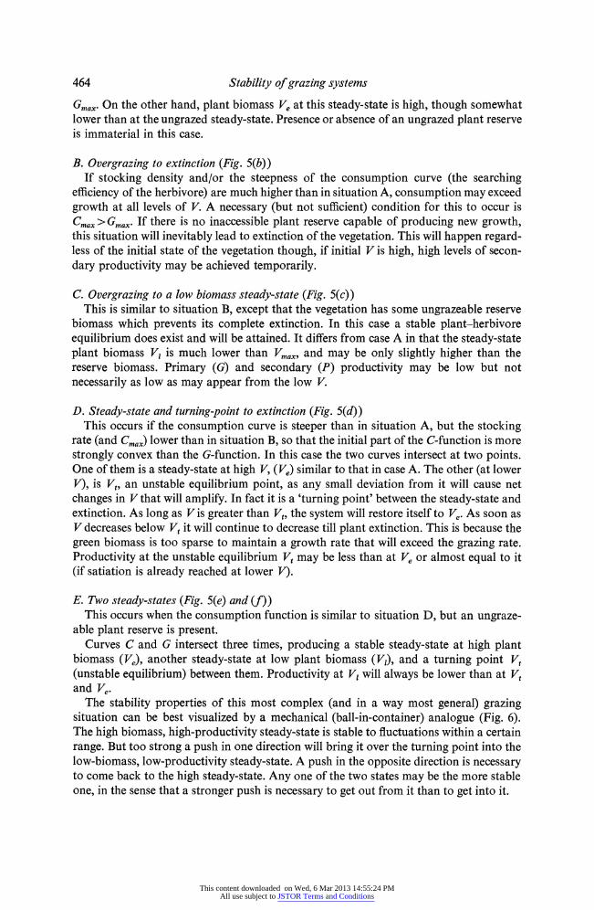
Gmax. On the other hand, plant biomass Ve at this steady-state is high, though somewhat lower than at the ungrazed steady-state. Presence or absence of an ungrazed plant reserve is immaterial in this case.

B. Overgrazing to extinction (Fig. 5(b)) If stocking density and/or the steepness of the consumption curve (the searching

efficiency of the herbivore) are much higher than in situation A, consumption may exceed growth at all levels of V. A necessary (but not sufficient) condition for this to occur is Cmax >Gmax. If there is no inaccessible plant reserve capable of producing new growth, this situation will inevitably lead to extinction of the vegetation. This will happen regard- less of the initial state of the vegetation though, if initial V is high, high levels of secondary productivity may be achieved temporarily.

C. Overgrazing to a low biomass steady-state (Fig. 5(c)) This is similar to situation B, except that the vegetation has some ungrazeable reserve

biomass which prevents its complete extinction. In this case a stable plant-herbivore equilibrium does exist and will be attained. It differs from case A in that the steady-state plant biomass V, is much lower than Vmax, and may be only slightly higher than the reserve biomass. Primary (G) and secondary (P) productivity may be low but not necessarily as low as may appear from the low V.

D. Steady-state and turning-point to extinction (Fig. 5(d)) This occurs if the consumption curve is steeper than in situation A, but the stocking

rate (and Cmax) lower than in situation B, so that the initial part of the C-function is more strongly convex than the G-function. In this case the two curves intersect at two points. One of them is a steady-state at high V, (Ve) similar to that in case A. The other (at lower V), is Vt, an unstable equilibrium point, as any small deviation from it will cause net changes in V that will amplify. In fact it is a 'turning point' between the steady-state and extinction. As long as V is greater than Vt, the system will restore itself to Ve. As soon as V decreases below V, it will continue to decrease till plant extinction. This is because the green biomass is too sparse to maintain a growth rate that will exceed the grazing rate. Productivity at the unstable equilibrium V, may be less than at Ve or almost equal to it (if satiation is already reached at lower V).

E. Two steady-states (Fig. 5(e) and (f)) This occurs when the consumption function is similar to situation D, but an ungraze-

able plant reserve is present. Curves C and G intersect three times, producing a stable steady-state at high plant

biomass (Ve), another steady-state at low plant biomass (V,), and a turning point V, (unstable equilibrium) between them. Productivity at V, will always be lower than at V, and Ve.

The stability properties of this most complex (and in a way most general) grazing situation can be best visualized by a mechanical (ball-in-container) analogue (Fig. 6). The high biomass, high-productivity steady-state is stable to fluctuations within a certain range. But too strong a push in one direction will bring it over the turning point into the low-biomass, low-productivity steady-state. A push in the opposite direction is necessary to come back to the high steady-state. Any one of the two states may be the more stable one, in the sense that a stronger push is necessary to get out from it than to get into it.




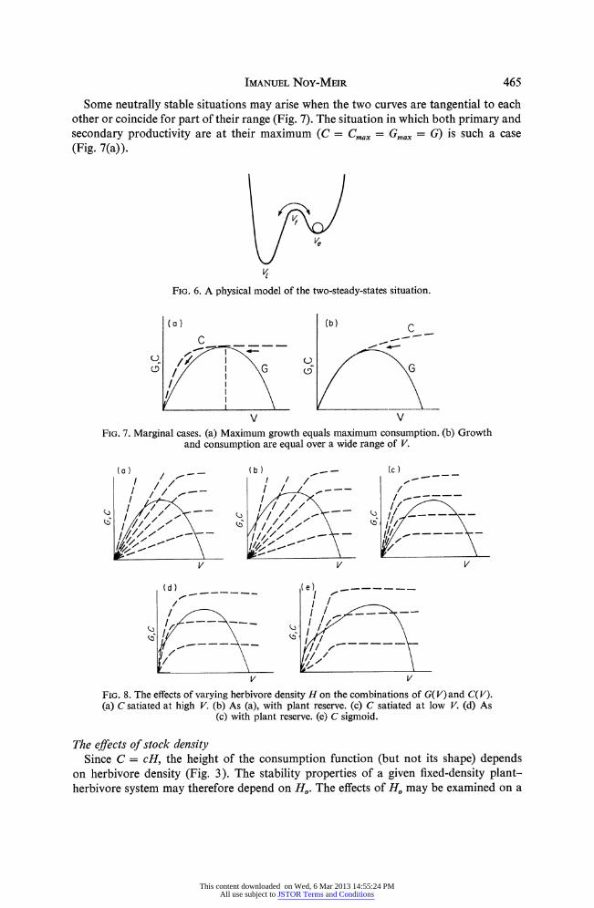
Some neutrally stable situations may arise when the two curves are tangential to each other or coincide for part of their range (Fig. 7). The situation in which both primary and secondary productivity are at their maximum (C = Cmx = Gmax = G) is such a case (Fig. 7(a)).

FIG. 6. A physical model of the two-steady-states situation.

(a) (b) C IC

( 9 , \ G ) G CD G

V V FIG. 7. Marginal cases. (a) Maximum growth equals maximum consumption. (b) Growth

and consumption are equal over a wide range of V.

(a) (b) -/ (c)

//I

t

/ /

I I /--- / ------

V V V

(d) (e) -

v v

FI. 8. The effects of varying herbivore density H on the combinations of G and CV). FIG. 8. The effects of varying herbivore density H on the combinations of G(V) and C( V). (a) C satiated at high V. (b) As (a), with plant reserve. (c) C satiated at low V. (d) As

(c) with plant reserve. (e) C sigmoid.

The effects of stock density Since C = cH, the height of the consumption function (but not its shape) depends

on herbivore density (Fig. 3). The stability properties of a given fixed-density plant- herbivore system may therefore depend on Ho. The effects of Ho may be examined on a




given G(V) graph superimposed on a family of C(V) graphs with different Ho (Fig. 8). The (V, Ho) values of the intersection points on this graph may also be plotted onto a 'phase graph' (H versus V; Fig. 9), to give the zero-change isocline of the vegetation, i.e. the line joining the combination of H and Vvalues at which plant biomass is not changing (Rosenzweig & MacArthur 1963).

These graphs show that, at low stocking rates, all conceivable plant-herbivore systems will be in situation A, i.e. will have a single, stable equilibrium point with high plant biomass. There are five possible responses of a system to increased Ho, depending on the shape of the consumption function c(V), and on the presence of an unconsumable plant reserve.

Case 1 With increased stocking rate the high steady state passes gradually into a low steady-

state, until a critical level of Ho where extinction occurs: A * C -* B (Figs 8(a) and 9(a)).

(a) l

(b) (c) low extinction extinction

( ds) extinction t-st exc)

Hlow s t-s t

., -H H st-st st-st

\ \ low st-st -iLX^.J s\yl -/t two two

l \ high - ? h~h ! ~-s hiSh st-sttst-st V V

FIG. 9. Possible responses of plant-herbivore systems to increased herbivore density: the isocline of zero plant growth in the V-H plane; (a)-(e) correspond to (a)-(e) in Fig. 8. (a) Continuously stable to extinction. (b) Continuously stable, no extinction. (c) Discontinu- ously stable between high- V steady-state and extinction. (d) Discontinuously stable between

high-V and low-V steady-states. (e) As (d), extinction also possible.

This will result when the consumption function is linear or nearly so in the range of V below V~, i.e. when the herbivore does not show any signs of satiation in this range.

Case 2 This case is similar to case 1 in that there is a gradual and continuous decrease in

steady-state V with increasing H (Figs 8(b) and 9(b)). It differs only in that complete extinction of the vegetation does not occur even at high stocking rates (A -* C), owing to the existence of an ungrazeable residual plant reserve or growth potential.

Case 3: A - D - B At low stocking rates there is a high steady-state, at very high ones there is extinction.

But at intermediate Ho the system is conditionally stable: it is stable as long as the amount




of vegetation is above a threshold V, and goes to extinction when V drops below it (Figs 8(c) and 9(c)). The higher the stocking density, the higher the critical level Vt.

Case 4: A -- E -- C This case differs from the previous one in the existence of a plant reserve. Thus a low

steady-state replaces extinction as the outcome of high stocking rates, or a drop below the critical V at intermediate ones (Figs 8(d) and 9(d)).

Case 5: A -B E - C -- B This case differs from case 4 in that, at very high stocking rates, there is a change from

a low steady-state to extinction (Figs 8(e) and 9(e)). It may occur if the consumption curve is sigmoid, or if there is a plant reserve not absolutely immune to grazing, or if it is exhaustible by continuous cropping of the growth produced by it.

(a) (b) (c)

P P P

M M M

H H H

(d) (e)

P P

M AM

H H

FIG. 10. Gross herbivore productivity at steady-state, P, as a function of herbivore density H. M is maintenance; net productivity is the difference between P and M. Cases (a)-(e) correspond to (a)-(e) in Figs 8 and 9. Broken vertical lines delimit the range of H

in which two alternative steady-states, with different P, are possible.

In general, plant-herbivore systems can thus be classified by two criteria: they may be divided into systems liable to extinction (cases 1, 3 and 5) and those not liable to extinction (2 and 4); and into systems which are continuously stable upon changes in H or V (1 and 2) and systems which are discontinuously stable (3, 4 and 5). Discontinuously stable systems are systems with more than one domain of attraction (Holling 1973) separated by a critical boundary ('rim'). Cases 4 and 5 may also be characterized as

systems which have two distinct non-zero steady-states, while 1, 2 and 3 have only one.

Productivity and animal density If it is assumed that gross animal productivity Pg is linearly proportional to total

consumption, its level at each equilibrium point can be read directly off graphs like Fig. 8. The dependence of C on stocking rate H for each type of plant-herbivore system can be read off Fig. 8 and plotted as a graph of C(Q Pg) against H (Fig. 10). The maintenance

requirements in such a graph are a straight line, so that the difference between the

P(H) curve and this line gives the net animal productivity (per unit area), Pn.




The effect of herbivore density on steady-state productivity is rather different in continuously stable and discontinuously stable systems. In continuously stable systems (Fig. 10(a) and (b)), productivity rises with increasing H to a maximum, then gradually decreases with further increase in H. Gross productivity may or may not reach zero at some level of H (depending on whether the vegetation is liable to extinction), but net steady-state productivity will always reach zero at some high H, beyond which net loss will occur. This P versus H curve is similar to some curves of production per unit area versus stocking rate which have been derived theoretically (Petersen, Lucas & Mott 1965; Owen & Ridgman 1968; Shaw 1970), and to some found experimentally (e.g. Harlan 1968).

The P(H) function predicted for discontinuously stable systems (Fig. 10(c), (d) and (e)) is similar only in the first part, increasing in a continuous convex form (i.e. decreasing marginal productivity with increased H) to a maximum. However, when H is increased beyond the level of maximum productivity, Hm (or a level slightly above it), steady-state productivity drops suddenly to a much lower level or even to zero. Furthermore, over a certain range of densities approaching Hm, productivity may also drop drastically if V is below a critical level V, either owing to initial conditions or to a chance fluctuation. Over this range of H, two levels of steady-state productivity are possible, depending on the history of the system.

Thus, in discontinuously stable grazing systems, animal productivity may remain very high even when the system is on the verge of a catastrophical collapse. In such a system, animal condition is not a sensitive indicator of the state of the system, as no deterioration in animal condition may be observed until after the crash. The level of plant cover V is the only sensitive indicator which can give warning of an approach to the critical threshold.

Fig. 10(d) and (e) also lead to some conclusions about the effects of stocking rate within the intermediate range where two levels of productivity are possible. The higher the stocking rate, the larger the difference in productivity between the two states, and the nearer is the theshold to the higher level (i.e. the higher the probability of a transition from high to low relative to a transition from low to high).

Effects of plant characteristics The characteristics of the plant in the grazing system affect the shape of both growth

and consumption functions, and through them the properties of the system. Simple graphical considerations (Fig. 11) lead to the following conclusions about the effects of various growth characteristics (other things being equal).

(a) An increase in the growth rate at all V, without change in the shape and position of the G(V) curve, results in higher productivity at all H and higher maximum H with which the vegetation can be in equilibrium. Such differences in the overall growth rates (faster-growing variety, higher temperature) do not affect the qualitative stability properties, i.e. whether the system is continuously or discontinuously stable, but they do affect threshold values. If it is discontinuously stable, there will be a discontinuous response of productivity and biomass to increased growth rate (g or Gmax) at constant H, if H is in the intermediate range.

(b) The level of Vmax and the steepness of the decline in G between Vx and Vmax does not affect qualitative stability, but only the relative sensitivity of the high steady-state to changes in H and V.




(c) The level of plant cover at which growth is maximal (Vx) and the slope and convexity of the initial response of G to V in the range of low V (at given Gmax) are critical to the stability of the system. Vegetation with high Vx and an initially flat (or concave) growth function is more likely to create discontinuous stability, over a wider range of H, than vegetation in which maximum growth is achieved at relatively low biomass and in which the approach of the G-function to this point is convex and initially steep. A change in the vegetation or the environment which increases Vmax and Gmax ('enrichment' or maximum productivity) but not the initial slope of G(V) ( = the maximum relative growth rate g) will raise Vx and therefore may turn a continuously stable system into a discontinuously stable one.

(d) The presence of an ungrazeable reserve biomass or a residual growth potential enables a vegetation to avoid extinction at high H and to maintain a low steady-state instead. Furthermore, the larger the reserve or the residual growth, the smaller is the

(a) _ (b) (c)

/ r 1/- 1/.---

2-2 / /

~~2 2

(d) ( (e)

2 2

V V

FIG. 11. The effects of plant characteristics on the combination of G(V) and C(V). (a) Varying g and Gmax. (b) Varying Vmax. (c) Varying V,,g, and the initial convexity of G(V). (d) The effect of a residual plant biomass or growth potential. (e) Varying the level of V

which allows herbivore consumption to be satiated.

chance of the vegetation being discontinuously stable under grazing, and the smaller the range of H in which discontinuity occurs (if at all).

(e) Vegetation attributes affect also the shape of the consumption curve. The steeper and more convex the curve, the easier it is for the herbivores to find and graze down the vegetation even when its biomass is already low; and the lower the level of Vat which the herbivore can graze enough to be satiated. Tall, erect vegetation will generally be more accessible to grazing at low V than low, prostrate vegetation (or vegetation that is taller than the herbivore itself), and therefore prone to 'crash' (discontinuous stability) over a wider range of H.

Effects of herbivore characteristics (a) The steepness and convexity of the consumption curve (in a given vegetation)

express the grazing efficiency of the herbivore, i.e. its ability to search, find and collect food at low levels of availability, and to maintain intake at or near maximum as plant




biomass decreases. Efficient grazers have steeper and more convex curves, and therefore are more likely to create discontinuously stable situations than inefficient grazers (Fig. 8) (e.g. sheep and goats versus cattle ?).

A sigmoid (initially concave) consumption function, such as may be caused by a 'learning' effect (Holling 1965), reduces the chances for discontinuous stability.

(b) The maximum intake rate per animal, Cmax, does not affect the shape of the consumption curve but only its height. Therefore its effects are identical to those of the stocking density H and the two parameters are interchangeable; only the product Cmax =

CmaxH is important (e.g. 2 animals with Cmax = 5 equal 5 animals with Cmax = 2). To this extent the practice of using 'animal units' to compare stocking rates in mixed herbivore situations (e.g. 1 cow = 5 sheep, 1 ram = 1.5 sheep) is justified. However, if the shape of the consumption curve is different these equivalence relations may be inapplicable and misleading at low V.

Effects of management practices (a) A policy of stock removal whenever V reaches a specified minimum (apart from

obviously precluding plant extinction) will generally reduce the range of H over which a crash can occur in a discontinuous system. But it will turn a discontinuous system into a continuous one only if the minimum is set to Vx (or higher).

(b) The effects of rotational versus continuous grazing cannot be included explicitly in the graphical analysis, which is based on continuous processes. However, a rough assessment can be made if we consider that rotation imposes fluctuations in H and V around the steady-state. If, in a discontinuously stable system the pasture is in a high steady-state under continuous grazing, such fluctuations can only push each division (in a grazing period) across the turning point towards extinction or a low steady-state. In the best case the divisions will recross the turning point during the rest period; but average production will certainly be lower. In the worst case the rest period will not be sufficient and the vegetation in each division in turn will remain trapped in the region around low steady-state or become extinct.

However, if the pasture is in a condition which under continuous grazing would maintain it in a low-production steady-state, rotation can be in certain cases beneficial. Then there is a chance that during a rest period each division crosses the turning point towards the high-production steady-state thus increasing average production. It may possibly remain on the high side even during the subsequent grazing periods.

The effects of rotation in discontinuously stable systems can be summarized by reference to the physical model (Fig. 6). If the ball is on the right (high-production) side, we may only lose by rocking it; but if it is on the left (low-production) side, we may only gain.

Similar predictions on the effects of rotation in a discontinuously stable system were obtained also by simulation experiments with an explicit growth-consumption model (Noy-Meir 1975).

In a continuously stable system there should be no significant difference between rotational and continuous grazing.

(c) A discontinuously stable system is highly labile at the stocking rate which allows the highest productivity (Fig. 7). Thus such a grazing system can be maintained at or near this maximum production rate only by very frequent, almost constant, adjustments of stock density in response to fluctuations in vegetation. A somewhat lower stocking rate will ensure more stable, though on the average somewhat lower, production.




Variable herbivore density Let us now replace assumption 9 (a constant Ho) by:

(9a) The effective herbivore density H changes in proportion to animal production and reproduction, which in turn is a function of available vegetation and herbivore density only.

This assumption may approach reality in extensive range systems, where animal numbers are not tightly controlled and depend mainly on natural reproduction and mortality.

In this case overall stability requires both H and V to be simultaneously stable. Thus in the H/V graph we must consider the zero-isocline of the herbivore (as well as that of the

plant), i.e. the set of H and V values at which there is no net change in herbivore density (AH = 0). Some possibilities are as follows.

(a) Net change in herbivore density depends only on vegetation availability; there is a certain level of vegetation Vs at which gross productivity, consumption and reproduc-

(a) (b) (c)

Hi // H/ A/ H/

Vs V V V

(d) (e)

H

H

V V

FIG. 12. The isocline of zero plant growth (continuous) and various forms of the isocline of zero herbivore growth (broken) in the V-H plane (after Rosenzweig & MacArthur 1963;

MacArthur & Connell 1966).

tion of the herbivores is balanced by the population 'maintenance' requirements (in- cluding mortality). When V is above this level, H increases; below it, it decreases. The herbivore isocline is a straight line (Fig. 12(a)). This is the simplest case treated in detail by Rosenzweig & MacArthur (1963) and MacArthur & Connell (1966).

(b) At high herbivore densities, their net increase is limited independently of the amount of vegetation available, e.g. by some other factor such as drinking water (Fig. 12(b)).

(c) Herbivore increase is limited at very low herbivore densities, e.g. by a decrease in mating probability (Fig. 12(c)).

(d) Herbivore net increase depends on the relation between available vegetation and herbivore density (i.e. the 'grazing pressure') so that the herbivore isocline is inclined (Fig. 12(d)).

(e) Various combinations (Fig. 12(e)).




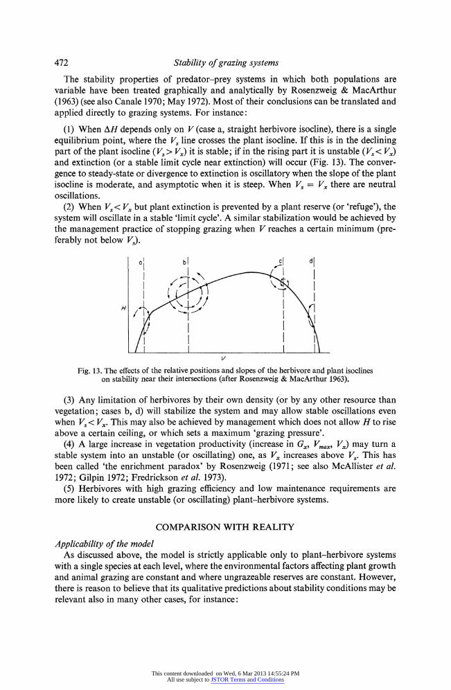
The stability properties of predator-prey systems in which both populations are variable have been treated graphically and analytically by Rosenzweig & MacArthur (1963) (see also Canale 1970; May 1972). Most of their conclusions can be translated and applied directly to grazing systems. For instance:

(1) When AH depends only on V (case a, straight herbivore isocline), there is a single equilibrium point, where the Vs line crosses the plant isocline. If this is in the declining part of the plant isocline (Vs > Vx) it is stable; if in the rising part it is unstable (Vs< Vx) and extinction (or a stable limit cycle near extinction) will occur (Fig. 13). The conver- gence to steady-state or divergence to extinction is oscillatory when the slope of the plant isocline is moderate, and asymptotic when it is steep. When Vs = Vx there are neutral oscillations.

(2) When Vs< Vx but plant extinction is prevented by a plant reserve (or 'refuge'), the system will oscillate in a stable 'limit cycle'. A similar stabilization would be achieved by the management practice of stopping grazing when V reaches a certain minimum (pre- ferably not below Vs).

a bl c| db

?i/

Fig. 13. The effects of the relative positions and slopes of the herbivore and plant isoclines on stability near their intersections (after Rosenzweig & MacArthur 1963).

(3) Any limitation of herbivores by their own density (or by any other resource than vegetation; cases b, d) will stabilize the system and may allow stable oscillations even when Vs < V,. This may also be achieved by management which does not allow H to rise above a certain ceiling, or which sets a maximum 'grazing pressure'.

(4) A large increase in vegetation productivity (increase in G,, Vx,,, Vx) may turn a stable system into an unstable (or oscillating) one, as Vy increases above Vs. This has been called 'the enrichment paradox' by Rosenzweig (1971; see also McAllister et al. 1972; Gilpin 1972; Fredrickson et al. 1973).

(5) Herbivores with high grazing efficiency and low maintenance requirements are more likely to create unstable (or oscillating) plant-herbivore systems.

COMPARISON WITH REALITY

Applicability of the model As discussed above, the model is strictly applicable only to plant-herbivore systems

with a single species at each level, where the environmental factors affecting plant growth and animal grazing are constant and where ungrazeable reserves are constant. However, there is reason to believe that its qualitative predictions about stability conditions may be relevant also in many other cases, for instance:




(a) More than one species is grazed but a single one is dominant; or there are several codominant species which do not differ greatly in growth and palatability characteristics.

(b) Plant growth and animal requirements vary with time, but change only moderately during a defined growth-and-grazing season. In this case the model may be applied to the stability of the interaction during this period alone, or to the overall stability if it depends critically on this period.

The model should at least help to understand this extended class of grazing systems, even those in which its predictions cannot be applied automatically and without some modifications. But in some other grazing systems its assumptions may be far from reality, for instance:

(a) Competition between two or more plants with very different growth and palatability is a dominant process. In this case there might be more than two equilibrium points (see Austin & Cook 1974).

15

3(G2)

t / % // \3a(GI)

2(\4) \ ^ 5 - 3b(G3)

200 400 600 800 V (g/m2)

FIG. 14. Plant growth in New Zealand ryegrass-clover pastures as function of biomass; curves reconstructed from experimental data by Brougham (1955, 1956). 1, May-June; 2, April; 3, October; 3a, October, ryegrass only; 3b, October, clover only (symbols in paren-

thesis for comparison with Table 1).

(b) Growth is seasonal but grazing is year-long, and the interactions in the period of grazing on dry vegetation are critical for plants (e.g. seeds) or animals. Then the combination of the two periods for overall stability could introduce qualitatively new features.

Bearing in mind these limitations, it is nevertheless worthwhile to search the extensive literature on grazing systems and experiments for evidence which would test the main predictions of the model, in particular about the special properties of discontinuously stable systems. A limited survey showed that most papers do not present information in a form suitable for this purpose. But there is some directly relevant quantitative information on intensive pastures, and some vaguer qualitative evidence from both pastures and extensive range.

Evidence from intensive (pasture) systems Firstly, it may be asked whether most real grazing systems are expected to have growth

and consumption functions leading to discontinuous stability, or to continuous stability.




Curves of growth as a function of green biomass may be reconstructed from data by Brougham (1955, 1956) on ryegrass-clover pastures in New Zealand (Fig. 14) and David- son & Donald (1958) on subterranean clover in Australia. Curves of intake as a function of green biomass are given by Willoughby (1959) for sheep on Phalaris-clover pasture, by Arnold (1963) for sheep on Phalaris-annuals-clover, and by Allden (1962) for sheep on ryegrass-clover (Fig. 15), all in Australia.

1500 3a

1000

3 3

500

200 400 600 V (g/m2)-

FIG. 15. Consumption per sheep as function of plant biomass; 1, Allden (1962), ryegrass- clover; 2, Willoughby (1959), Phzalaris-clover; 3, Arnold (1963), Phalaris-annuals-clover;

3a, winter-shorn sheep.

100

"EJ 61 t ffy^ >-^:>:<:1C2

~ 500 o. / V // \

__I I I /

100 200 300 400 V (g/m2)

FIG. 16. Superimposition of experimental growth and consumption curves, standardized to Gmax = Cmax m= 100%. GI, ryegrass in New Zealand, October (Brougham 1956); G6, subterranean clover in Australia, October (Davidson & Donald 1958). Consumption by

sheep: Cl (Allden 1962); C2 (Willoughby 1959); C3 (Arnold 1963).

By superimposing some of these growth and consumption curves, standardized by the maximum growth and consumption rates (Fig. 16), it can be seen which combinations would be continuously stable and which discontinuously stable (C greater than G over a range just below Vx). The results (Table 1) show that animals with the consumption curve reported by Allden would allow continuous stability in such pastures at all seasons




given. The New Zealand ryegrass pasture in June (possibly also in April) and the Australian subterranean clover in October would be continuously stable with all animals given. However, the sheep tested by Willoughby and Arnold would cause discontinuous stability in October in ryegrass, ryegrass-clover, and possibly in clover pastures.

Table 1. Stability conditions that would arise from superimposition of various observed growth and consumption functions of sheep on grass and clover

pastures G1-G6: growth functions (see Fig. 14). C1-C3: consumption functions (see Figs 15 and 16). Entries in table: C, continuous stability; D, discontinuous stability.

Growth function G1 G2 G3 G4 G5 G6

Consumption C1 C C C C C C function C2 D D C C C C

C3 D D D C? C C

In general it seems that discontinuous stability is quite possible (though not necessary) with sheep grazing pastures of these types.

The most striking and direct evidence for discontinuous stability in an intensive pasture has been presented by Morley (1966a), in a careful analysis of the results from a replicated grazing experiment with sheep at 3 stocking rates x 2 grazing systems (continuous and rotational) x 3 replicates. The variation in sheep liveweight per plot (in

SR Fig. 17 Fig. 18

I SFSR4 u 5 * * /

?z 6 _ _ He \

U7 ***/^ --- ^ -

6 ? e / 7 July liveweit ()

July liveweight (kg) Availability

FIG. 17. Results of a replicated grazing experiment (from Morley 1966a). SR (stocking rate) = 5, 6, 7 ewes/acre; ROTAT, 3-paddock rotation; CONT, continuous grazing.

FIG. 18. Plant growth and animal consumption as functions of plant availability and stocking rate, showing stable and unstable equilibria (from Morley 1966a).

winter) between replicates within some treatments (moderate and high continuous stocking) was usually high and showed a bimodal, or discontinuous distribution (Fig. 17). Morley concluded that animal performance was a 'threshold' or 'crash' function of stocking rate. At stocking rates near the threshold small differences in plant productivity between plots caused large differences in animal response. This led to a compre- hensive analysis of the factors affecting stability of production in pasture systems. The effects on stability of the functions relating plant growth and animal consumption to leaf area (plant availability) were discussed with reference to a graph of a discontinuously stable system (Fig. 18). Finally Morley (1966a, b) pointed out that a conventional statistical analysis of 'average effects' would have masked the discontinuity in the results

G




(and the theoretical insight derived from them). Thus it is possible that similar effects have been overlooked in the results from other grazing experiments.

Evidence from extensive (range) systems Direct experimental evidence from range systems is almost non-existent; even quanti-

tative observations which could be relevant to testing the model are very scarce. Further- more, range systems are usually much more complex than intensive pastures and the factors dominating their stability may often be quite different from those considered in this model (e.g. species composition, erosion). Nevertheless, it is interesting (though certainly not conclusive) that some qualitative observations on ranges, and some concepts in range management, are at least consistent with the possibility of discontinuous stability and some of the features associated with it.

Safe stocking rate. The distinction between 'safe' and 'maximal' stocking rate or carrying capacity, which is sometimes made by range managers on the basis of experience (e.g. Stoddart 1960), implies that at the stocking rate at which steady-state productivity is highest, it is also less stable than at somewhat lower stocking. This is true for discontinuously stable grazing systems (Figs 7(a), 10(c), (d) and (e)).

Range readiness. A practice much recommended by range experts is to delay the introduction of animals onto a range for some weeks after growth starts, until some minimum foliage builds up (Stoddart & Smith 1955). Such a practice would be critical in discontinuously stable systems, where it could mean the difference between a low-productivity and a high-productivity steady-state (at the same stocking rate) throughout the season. The point of 'range readiness' should then be just above the 'turning point' Vt between the two equilibria.

Grazing pressure. Grazing pressure is often defined as the ratio of stocking rate to available pasture, HIV, and considered by range managers to be a more significant para- meter than either H or V separately (e.g. Mott 1961). In the H versus V plot, points of equal grazing pressure are on a straight line passing through the origin, the slope of which depends on the grazing pressure. In a discontinuously stable system the critical biomass threshold V, increases with H, so that the range of critical values (the unstable part of the plant isocline) may be well approximated by a constant 'critical grazing pressure' (e.g. in Fig. 9(d) and (e)).

Forage condition v. animal condition as indicators. Range scientists claim that the cover or 'vigour' of the main palatable plants is a better indicator of the state of the range system than the animal condition. 'Research has shown that range deterioration may progress for considerable time before the change is reflected in livestock condition. Forage condition is a more sensitive indicator' (Stoddart & Smith 1955). One prediction by the model for discontinuously stable systems was that animal productivity may remain high just up to the 'crash point' (Fig. 10).

Effects of rotation. The reports on the effects of rotational versus continuous grazing on plant and animal production are conflicting, yet it seems that one generalization is possible (Heady 1961): rotational grazing is often beneficial in restoring deteriorated ranges to high productivity, while in ranges in good condition it usually results in lower productivity than continuous grazing (or at best the same). This again is consistent with what is expected for discontinuously stable systems (see above).

Discontinuities in range productivity. Paulsen & Ares (1961) presented data on the changes in vegetative cover and on range productivity (expressed as annual surface-acre requirement for one animal) over 40 years in subdivisions of the Jornada Experimental




Brush pastures Grass pastures

300 Pasture 6 Pasture 5

00 -

jo E 0

w 300 -Pasture I -Pasture 9

200 -

E_ 100L?lila_

or

300r- Posture 2 -Posture 10

200-

100 4

I 300 -Tl li

4^Tnp~I ,ilil, ̂ ,?1TTTt,,t,!TUTTTI 1916 20 24 28 32 36 40 44 48 1952 1916 20 24 28 32 36 40 44 48 1952

Grazing year

lo i

E /

oo 5 /j N / ' /

500 West Kimberley W.A.

400 -

0oo o I\. \ cI \ [

/3I I

~ 200 - U)

/ 100

1860 1900 1960

FIG. 20. Fluctuations in animal numbers in districts of arid Australia (from Perry 1968).




Range in semi-arid new Mexico. Fluctuations in cover generally follow rainfall fluctuations. Productivity in most plots shows a smooth trend with small fluctuations (10-30%) except for a few dry years in which there is a sudden decrease by a factor of 2-4 (Fig. 19) which is much greater than the decrease in rainfall. This might indicate discontinuous stability.

Perry (1968) presented graphs of sheep and cattle populations in regions of arid Aus- tralia from the time of settlement. The yearly fluctuations in each region seem for some periods to be around a high steady-state level (immediately after settlement, or after improvement in management) and for subsequent periods around a 'low' level, which is lower by a factor of 2-3 (Fig. 20). The drop from high to low densities is rather sudden and occurs in a severe drought.

Finally, some general concepts and phrases which are widely used by range ecologists and managers, and which are presumably based on experience, implicitly indicate an awareness of the possibility of discontinuous stability. Such are any references to the 'precarious ecological balance' or 'equilibrium' of the range, which may be 'upset' by overgrazing, even if temporary, leading to the initiation of 'range deterioration' which can be irreversible, or reversible only by special treatment.

While each of these pieces of evidence is rather meagre, cumulatively they indicate that some (probably many, though certainly not all) range and pasture systems are discontinuously rather than continuously stable. The graphical production-consumption model presented here offers one very simple hypothesis to explain such phenomena. However, many of them could have been caused by different mechanisms, in particular by changes in species composition.

CONCLUSIONS

The graphical analysis of stability of predator-prey systems is a rather theoretical approach developed by theoretical population ecologists (Rosenzweig & MacArthur 1963). Applied to a simple plant-herbivore model, this approach has yielded a series of general conclusions about stability and productivity. These appear to be relevant at least to some classes of real-world pastoral systems and to some problems in their practical management. Some of the conclusions are very similar to those reached by a pasture ecologist in a theoretical analysis spurred by some strange experimental results (Morley 1966a). The far-reaching implications of that analysis may not have been fully appreciated yet by most pasture scientists and managers.

The analytical techniques used here were the most rudimentary. More sophisticated mathematical techniques are available and are beginning to be applied to population systems. With them it should be possible to analyse somewhat more complex (and more realistic) models of grazing systems than the very simple one presented here; also more detailed conclusions may be possible. Anyway, the fact that even the simplest techniques and simplest model can give interesting results relevant to real pastoral systems is encouraging.

These preliminary results suggest that much more contact and feedback between the two disciplines of pasture and range ecology, and theoretical population ecology, could be useful to both sides. Theoretical ecologists could find in commercial grazing systems and in grazing experiments at least inspiration for new ideas and probably also oppor- tunities for field tests of models of population systems at several trophic levels. Pasture ecologists and practical workers could look to theoretical ecology at least for a broader




and clearer understanding of the problems of grazing systems, and probably also for guidelines to their management.

ACKNOWLEDGMENTS

I am grateful to Dan Cohen, Noam Seligman and Dan Wallach for their useful comments on the draft of the paper and to Peter Grossmann for drawing the figures.

This work was partly supported by Ford Foundation Grant 7/E-3 through Israel Foundations Trustees.

SUMMARY

A general model of simple grazing systems can be based on the general form of the functions relating both plant growth and herbivore consumption to vegetation biomass.

Graphical considerations lead from this model to predictions on the existence and number of plant-herbivore equilibrium points, whether they are stable or unstable and the relations between herbivore density, plant biomass and productivity at these points. Some predictions can be transferred directly from the existing theory of predator-prey graphs to plant-herbivore systems, while others need to be modified. The stability of

grazing systems depends on animal density and plant biomass either continuously, or

discontinuously, depending on the properties of the vegetation and the herbivore. Evidence from real pasture and range systems suggests that at least some of them are discontinuously stable, with significant implications for their management.

REFERENCES

Allden, W. G. (1962). Rate of herbage intake and grazing time in relation to herbage availability. Proc. Aust. Soc. Anim. Prod. 4, 163-6.

Arnold, G. W. (1963). Factors within plant associations affecting the behaviour and performance of grazing animals. Grazing in Terrestrial and Marine Environments (Ed. by D. J. Crisp), pp. 133-54. Blackwell Scientific Publications, London.

Austin, M. P. & Cook, B. G. (1974). Ecosystem stability: a result from an abstract simulation. J. theor. Biol. 45, 435-58.

Brougham, R. W. (1955). A study in rate of pasture growth. Aust. J. agric. Res. 6, 804-12. Brougham, R. W. (1956). The rate of growth of short-rotation ryegrass pastures in the late autumn, winter

and early spring. N.Z. Jl Sci. Technol. A38, 78-87. Canale, R. (1970). An analysis of models describing predator-prey interaction. Biotechnol. Bioeng. 12,

353-78. Davidson, J. L. & Donald, C. M. (1958). The growth of swards of subterranean clover with particular

reference to leaf area. Aust. J. agric. Res. 9, 53-72. Donald, C. M. (1961). Competition for light in crops and pastures. Mechanisms in Biological Competition

(Ed. by F. L. Milthorpe). Symp. Soc. exp. Biol. 15, 282-313. Gilpin, M. E. (1972). Enriched predator-prey systems: theoretical stability. Science, N.Y. 177, 902-4. Fredrickson, A. G., Jost, J. L., Tsuchiya, H. M. & Hsu, P-H. (1973). Predator-prey interactions between

Malthusian populations. J. theor. Biol. 38, 487-526. Harlan, J. R. (1958). Generalized curves for gain per head and gain per acre in rates of grazing studies.

J. Range Mgmt, 11, 140-7. Heady, H. F. (1961). Continuous vs. specialized grazing systems. A review and application to the Cali-

fornia annual type. J. Range Mgmt, 14, 182-93. Holling, C. S. (1965). The functional response of predators to prey and its role in mimicry and population

regulation. Mem. Entomol. Soc. Can. No. 45, 1-60. Holling, C. S. (1966). The functional response of invertebrate predators to prey density. Mem. Entomol.

Soc. Can. No. 48, 1-86. Holling, C. S. (1973). Resilience and stability of ecological systems. A. Rev. Ecol. Syst. 4, 1-24. Hubell, S. P. (1973). Populations and simple foodwebs as energy filters. I. One-species systems. II. Two-

species systems. Am. Nat. 107, 94-121, 122-51.




Ivlev, V. S. (1961). Experimental Ecology of the Feeding of Fishes. Yale University Press, New Haven. McAllister, C. D., Le Brasseur, T. R. & Parsons, T. R. (1972). Stability of enriched aquatic ecosystems.

Science, N. Y. 175, 562-5. MacArthur, R. M. & Connell, J. H. (1966). The Biology ofPopulations. Wiley, New York. Maly, E. J. (1969). A laboratory study of the interaction between the predatory rotifer Asplanchia and

Paramecium. Ecology, 50, 59-73. May, R. M. (1971). Stability in model ecosystems. Proc. ecol. Soc. Aust. 6, 18-56. May, R. M. (1972). Limit cycles in predator-prey communities. Science, N.Y. 177, 900-2. Maynard Smith, J. & Slatkin, M. (1973). The stability of predator-prey systems. Ecology, 54, 384-91. Morley, F. H. W. (1966a). Stability and productivity of pastures. Proc. N.Z. Soc. Anim. Prod. 26, 8-21. Morley, F. H. W. (1966b). The biology of grazing management. Proc. Aust. Soc. Anim. Prod. 6, 127-36. Mott, G. 0. (1961). Grazing pressure and the measurement of pasture production. Proc. VIII int. Grassld

Congr. pp. 606-11. Alden Press, Oxford. Noy-Meir, I. (1975). Rotational grazing in a continuously growing pasture: a simple model. J. agric.

Syst. 1 (in press). Owen, J. B. & Ridgman, W. J. (1968). The design and interpretation of experiments to study animal

production from grazed pasture. J. agric. Sci., Camb. 71, 327-35. Paulsen, H. A. & Ares, F. N. (1961). Trends in carrying capacity and vegetation on arid southwestern

range. J. Range Mgmt, 14, 78-83. Perry, R. A. (1968). Australia's arid rangelands. Ann. Arid Zone, 7, 243-9. Petersen, R. G., Lucas, H. L. & Mott, G. 0. (1965). Relationship between rate of stocking and per animal

and per acre performance on pasture. Agron. J. 57, 27-30. Rosenzweig, M. L. (1969). Why the prey curve has a hump. Am. Nat. 103, 81-7. Rosenzweig, M. L. (1971). The paradox of enrichment: destabilization of exploitation ecosystems in

ecological time. Science, N. Y. 171, 385-7. Rosenzweig, M. L. (1973). Exploitation in three trophic levels. Am. Nat. 107, 275-94. Rosenzweig, M. L. & MacArthur, R. H. (1963). Graphic representation and stability conditions of

predator-prey interactions. Am. Nat. 97, 209-23. Salt, G. W. (1967). Predation in an experimental protozoan population (Woodruffia-Paramecium).

Ecol. Monogr. 37, 113-44. Shaw, N. H. (1970). The choice of stocking rate treatments as influenced by the expression of stocking

rate. Proc. XI int. Grassld Congr. pp. 909-13. University of Queensland Press, Brisbane. Stoddart, L. A. (1960). Determining correct stocking rate on range land. J. Range Mgmt, 13, 251-5. Stoddart, L. A. & Smith, A. D. (1955). Range Management, 2nd edn. McGraw-Hill, New York. Strebel, D. E. & Goel, N. S. (1973). On the isocline methods for analyzing prey-predator interactions.

J. theor. Biol. 39, 211-39. Vandermeer, J. H. (1973). Generalized models of two species interactions: a graphical analysis. Ecology,

54, 809-18. Willoughby, W. M. (1959). Limitations to animal production imposed by seasonal fluctuations in pasture

and by management procedures. Aust. J. agric. Res. 10, 248-68. Wit, C. T. de, Brouwer, R. & Penning de Vries, F. W. T. (1970). The simulation of photosynthetic systems.

Prediction and Measurement of Photosynthetic Productivity: Proc. IBP/PP Techn. Meeting, Trebon, pp. 47-70. Pudoc, Wageningen.

(Received 15 August 1974)

LIST OF SYMBOLS

c Consumption (intake) rate per animal Cmax Maximum (satiation) consumption rate per animal C Consumption rate (by herbivore population at given H) per unit area Cmax Maximum consumption per unit area G Plant growth rate (biomass/time) Gmax = Gx Maximum growth rate Gr Residual growth rate when V = 0 g Maximum relative growth rate H Herbivore density Ho Fixed level of herbivore density




Hm Maximum herbivore density that can be in equilibrium with vegetation m Maintenance rate per animal (in productivity units) M Maintenance rate of herbivore population per unit area P = Pg Gross productivity of herbivore population per unit area Pn Net productivity of herbivore population per unit area V Plant biomass per unit area Vmax Maximum plant biomass Vx Plant biomass at which growth is maximal Ve Equilibrium plant biomass (high level) VI Equilibrium plant biomass (low level) Vt Critical threshold (turning point) of plant biomass Vs Plant biomass density sufficient for herbivore population maintenance Vr Residual (ungrazed) plant biomass



Documents

Stability of Grazing Systems: An Application of Predator-Prey Graphs · 2013-11-11 · STABILITY OF GRAZING SYSTEMS: AN APPLICATION OF PREDATOR-PREY GRAPHS ... Some explicit forms