Stability control and protection of power systems with VSC

STABILITY CONTROL AND

PROTECTION OF POWER SYSTEMS

WITH VSC HVDC AND VSC FACTS

by

RUI GUAN

A thesis submitted to

The University of Birmingham

for the degree of

DOCTOR OF PHILOSOPHY

Department of Electronic,

Electrical and Systems Engineering

The University of Birmingham

March 2018

University of Birmingham Research Archive

e-theses repository This unpublished thesis/dissertation is copyright of the author and/or third parties. The intellectual property rights of the author or third parties in respect of this work are as defined by The Copyright Designs and Patents Act 1988 or as modified by any successor legislation. Any use made of information contained in this thesis/dissertation must be in accordance with that legislation and must be properly acknowledged. Further distribution or reproduction in any format is prohibited without the permission of the copyright holder.

To my parents

ACKNOWLEDGEMENTS

Foremost, I would like to express my deepest gratitude to my supervisor, Prof. Xiao-Ping

Zhang. It is his invaluable guidance and devoted support that encourages my pursuit of

research achievements. His pioneering foresight and cognition of energy internet has formed

the foundation of my research goal. His patient guidance and advanced resources has

provided me with the platform to carry out my study. There would be no chance that I can

manage to complete this thesis and related academic achievements, without his

professionalism and dedication. I am truly privileged to study in his research group.

This Ph.D. study was partly sponsored by Department of Electronic, Electrical and Systems

Engineering, School of Engineering, University of Birmingham. I would like to acknowledge

my gratitude for the financial support.

I would also like to thank my colleagues Dr. Dechao Kong, Dr. Suyang Zhou, Dr. Jingchao

Deng, Dr. Jianing Li, Dr. Puyu Wang, Dr. Na Deng, Dr. Jing Li, Dr. Ying Xue, Dr. Zhi Wu,

Dr. Can Li, Dr. Mingyu Xie, Dr. Hao Fu, Dr. Conghuan Yang, Mr. Zuanhong Yan, Mr. Mao

Li, Miss Xianxian Zhao, Mr. Jiajie Luo, and Mr. Min Zhao from the Electrical Power and

Control Systems Group for their kind advices and inspiring discussions. It has been a

beneficial experience to work with them over the past three years.

Last but not least, I would like to thank my beloved parents, Mr Jun Guan and Mrs. Cuili

Shang and all of my family members. I am deeply grateful for their devotion and support

through my whole research period. They have made me who I am.

I

ABSTRACT

The recent progress of high-voltage high-power fully controlled semiconductor technology

laid the foundation of voltage source converter (VSC) technology, which continues to

advance the developments of high voltage direct current (HVDC) technology and flexible

alternating current transmission systems (FACTS). Nowadays, due to the ever increasing

amount of the integration of renewable energy sources into power systems and the demand of

long-distance bulk power transmission with enhanced power system controllability and

increased power transfer capability, VSC converter based technology (in particular, VSC

HVDC and VSC FACTS) has been applied as a crucial solution to these big challenges.

However, the high penetration of these VSC based systems may introduce certain risks to

existing power systems in two primary aspects: dynamic stability and protection. This thesis

investigates the impacts of VSC HVDC and VSC FACTS on system dynamic stability and

protection.

VSC based HVDC system is the preferred solution for grid connection of large-scale offshore

wind farms, as it is a feasible option for long distance submarine interconnection of passive

and weak systems. With increasing installations of VSC HVDC systems in power grids, the

investigation of controllability and stability of VSC-based multi-terminal direct current

(MTDC) systems becomes important as it benefits the existing AC systems with a means of

increased energy transfer between interconnected system operators. However, for VSC-based

MTDC systems, the current flow control of DC grid has become a challenge, with more

installed and planned applications of multi-terminal HVDC transmission systems. The DC

current flow controller (CFC) is a DC-DC converter based power flow control solution which

can provide multi-line flexible current flow control in a simple meshed DC network. Small-

signal stability analysis has been widely used for the study of system dynamics and design of

controllers for VSC converters. However, the most of the published research papers on small-

signal stability of VSC MTDC systems have mainly been focused on the dynamics of the

VSC while there is a lack of considerations of the potential impacts of DC power-flow

controller on existing MTDC systems in terms of system stability and dynamic performance

under disturbances. And there is a real need to fill in the gap of the study of interactions

between DC networks with CFC and VSC converters (even more broadly, the detailed

representation of connected AC networks). In this thesis, an integrated small-signal stability

II

model for the study of interactions between CFC and VSC is established. Modal analysis

results are verified by simulation results from real time digital simulations (RTDS) under

both small and large AC/DC disturbances. The impacts of control parameters of CFC on the

integrated AC/DC system and the interactions between VSC and CFC are investigated using

both modal analysis and time-domain simulations.

The emerging VSC FACTS devices are commonly regarded as an effective solution for fast-

response voltage/reactive power support during normal and fault conditions. However, the

implementation of VSC FACTS (for instance, STATCOM) and VSC HVDC in high voltage

transmission systems may introduce certain potential risks or impacts to the existing

protection and control systems. Unexpected changes of the impedance measurements due to

the integration of VSC-FACTS and VSC HVDC may trigger mal-operation of feeder distance

protection of AC systems, since the performance of feeder distance protection is heavily

dependent on the impedance measurements. The mathematical representation of the apparent

impedance measurement of distance relay is derived considering the infeed current from VSC

HVDC and VSC FACTS at different locations. The apparent impedance measurements

analysis and dynamic simulation study are performed to investigate the impacts of VSC

HVDC and VSC FACTS on distance protection. A RTDS-based hardware-in-loop testing

platform is established using practical distance relays and detailed model of VSC HVDC and

multiple VSC FACTS. The impacts of VSC HVDC and VSC FACTS on feeder distance

protection are investigated, based on different types of internal/external fault test simulation

occurred at various locations.

In this thesis, a small-signal stability model of the integrated AC/DC systems with VSC and

CFC is presented to characterize modes and investigate various control parameters of CFC on

the eigenvalue trajectories of system modes. Small-signal stability analysis is performed to

investigate the interactions between CFC and VSC. The mathematical representation of the

apparent impedance measurements of feeder distance relays against various fault scenarios is

derived considering the infeed current from VSC HVDC and VSC FACTS at different

locations.

III

TABLE OF CONTENTS

CHAPTER 1 INTRODUCTION ............................................................................................ 1

1.1 Research Background ...................................................................................................... 1

1.1.1 VSC HVDC .............................................................................................................. 1

1.1.2 VSC FACTS ............................................................................................................. 9

1.1.3 CFC in MTDC ........................................................................................................ 10

1.1.4 Distance Protection ................................................................................................. 12

1.2 Literature Review........................................................................................................... 14

1.2.1 Modelling and Control of VSC HVDC and VSC FACTS ..................................... 14

1.2.2 Small-Signal Stability Analysis of VSC MTDC .................................................... 18

1.2.3 Impacts of VSC HVDC and VSC FACTS on Distance Protection ........................ 20

1.3 Research Focuses and Contributions ............................................................................. 22

1.3.1 Research Focuses .................................................................................................... 22

1.3.2 Scientific Contributions of the Thesis..................................................................... 22

1.4 Outline of the Thesis ...................................................................................................... 23

CHAPTER 2 SMALL-SIGNAL STABILITY ANALYSIS OF VSC BASED MTDC

SYSTEM WITHOUT DC CFC ............................................................................................ 25

2.1 Introduction .................................................................................................................... 25

2.2 Modelling of AC Power System .................................................................................... 25

2.2.1 Synchronous Generator with Excitation System and PSS ...................................... 26

2.2.2 Network Power Flow .............................................................................................. 30

2.3 Modelling of MTDC System without CFC ................................................................... 31

2.3.1 VSC with Its Control System .................................................................................. 31

2.3.2 DC Network without CFC ...................................................................................... 37

2.4 Linearization and Formulation of Multi-Model System ................................................ 39

2.4.1 Linearization of AC Power System ........................................................................ 40

IV

2.4.2 Linearization of MTDC System without CFC ........................................................ 43

2.4.3 Formulation of Multi-Model System ...................................................................... 45

2.5 Small-Signal Stability Analysis ..................................................................................... 46

2.5.1 Test System ............................................................................................................. 47

2.5.2 Modal Analysis ....................................................................................................... 48

2.6 Simulation Validation .................................................................................................... 52

2.6.1 Small Disturbances ................................................................................................. 53

2.6.2 Large Disturbances ................................................................................................. 57

2.7 Summary ........................................................................................................................ 65

CHAPTER 3 SMALL-SIGNAL STABILITY ANALYSIS OF VSC BASED MTDC

SYSTEM WITH DC CFC ..................................................................................................... 66

3.1 Introduction .................................................................................................................... 66

3.2 Modelling, Linearization and Formulation of VSC Based MTDC System with CFC .. 66

3.2.1 Modelling of DC Network with CFC ..................................................................... 67

3.2.2 Linearization of DC Network with CFC ................................................................. 71

3.2.3 Formulation of Multi-Model System ...................................................................... 72

3.3 Impacts of CFC on Small-Signal Stability of the Integrated AC/DC System ............... 73

3.3.1 Test System ............................................................................................................. 73

3.3.2 Modal Analysis ....................................................................................................... 74

3.3.3 Impacts of Control Parameters of CFC ................................................................... 78

3.3.4 Dynamic Simulation Validation ............................................................................. 81

3.4 Interactions between CFC and VSC .............................................................................. 87

3.4.1 Impacts of Control Parameters of CFC on VSC ..................................................... 87

3.4.2 Impacts of Control parameters of VSC on CFC ..................................................... 90

3.5 Summary ........................................................................................................................ 93

CHAPTER 4 IMPACTS OF VSC HVDC SYSTEM ON DISTANCE PROTECTION . 96

4.1 Introduction .................................................................................................................... 96

V

4.2 Distance Protection of Two-Ended Overhead Transmission Lines ............................... 96

4.2.1 Basic Principles of Distance Protection .................................................................. 96

4.2.2 Zones of Protection ................................................................................................. 98

4.2.3 Distance Relay Characteristics ............................................................................... 99

4.2.4 Under-reach and Over-reach Effect of Distance Relay Application .................... 102

4.3 Impacts of VSC HVDC System on Distance Protection ............................................. 103

4.4 Dynamic Simulation Study .......................................................................................... 108

4.4.1 Establishment of RTDS-based Hardware-in-Loop Testing Platform ................... 108

4.4.2 Test System with VSC HVDC and Protection Relay Settings ............................. 109

4.4.3 Dynamic Simulation Result of Test System without/with VSC HVDC .............. 110

4.5 Summary ...................................................................................................................... 114

CHAPTER 5 IMPACTS OF VSC FACTS ON DISTANCE PROTECTION ............... 116

5.1 Introduction .................................................................................................................. 116

5.2 Modelling of STATCOM ............................................................................................ 116

5.2.1 Configuration of STATCOM ................................................................................ 116

5.2.2 Control System of STATCOM ............................................................................. 118

5.3 Impacts of STATCOM on Distance Protection ........................................................... 123

5.3.1 Analysis of Internal Faults .................................................................................... 123

5.3.2 Analysis of External Faults ................................................................................... 128


5.4.1 Test System with VSC FACTS and Protection Relay Settings ............................ 134

5.4.2 Dynamic Simulation Results of Test System against Internal Faults ................... 135

5.4.3 Dynamic Simulation Results of Test System against External Faults .................. 141

5.5 Summary ...................................................................................................................... 146

CHAPTER 6 COMBINED IMPACTS OF VSC HVDC AND VSC FACTS ON

DISTANCE PROTECTION ............................................................................................... 149

6.1 Introduction .................................................................................................................. 149

VI

6.2 Impacts of VSC HVDC and VSC FACTS on Distance Protection ............................. 149

6.2.1 VSC HVDC and VSC FACTS Connected to Different Buses ............................. 149

6.2.2 VSC HVDC and VSC FACTS Connected to Same Bus ...................................... 155

6.2.3 VSC HVDC and Multiple VSC FACTS ............................................................... 160


6.3.1 Test System with VSC HVDC and VSC FACTS and Protection Relay Settings 163

6.3.2 Dynamic Simulation Results of Test System with VSC HVDC and VSC FACTS at

Different Locations ........................................................................................................ 164

6.4 Summary ...................................................................................................................... 170

CHAPTER 7 CONCLUSIONS AND FUTURE WORK ................................................. 173

7.1 Conclusions .................................................................................................................. 173

7.2 Future Work ................................................................................................................. 176

APPEDNDIX A .................................................................................................................... 177

A.1 Generator Parameters .................................................................................................. 177

A.2 Excitation System Parameters ..................................................................................... 177

A.3 PSS Parameters ........................................................................................................... 177

A.4 Transmission Line Parameters .................................................................................... 178

A.5 Generation Data .......................................................................................................... 178

A.6 Load Data .................................................................................................................... 178

A.7 VSC Parameters .......................................................................................................... 179

A.8 DC Network Parameters ............................................................................................. 179

A.9 CFC Parameters .......................................................................................................... 179

APPENDIX B ....................................................................................................................... 180

B.1 Transmission Line Parameters .................................................................................... 180

B.2 Equivalent Voltage Sources and Internal Impedance Parameters ............................... 180

LIST OF PUBLICATIONS & OUTCOMES .................................................................... 181

REFERENCES ..................................................................................................................... 182

VII

LIST OF FIGURES

Figure 1- 1 Global demand for different forms of primary energy (2010 – 2050) [5]. ............ 1

Figure 1- 2 Structure of global end-use energy consumption (2010 – 2050) [5]. .................... 3

Figure 1- 3 Configuration of VSC HVDC. ............................................................................... 4

Figure 1- 4 Topology of a two-level three-phase bridge inside VSC. ...................................... 5

Figure 1- 5 Topology of a three-level VSC. ............................................................................. 6

Figure 1- 6 Waveforms associated with PWM and voltage of a two-level converter. ............. 6

Figure 1- 7 Topology of a MMC. ............................................................................................. 7

Figure 1- 8 Configuration of a half-bridge SM. ........................................................................ 7

Figure 1- 9 Converter voltage creation of two-level VSC, three-level VSC and MMC. ......... 8

Figure 1- 10 Configuration of a two-level star-connection STATCOM. ............................... 10

Figure 1- 11 Topology of a two-line CFC. ............................................................................. 12

Figure 1- 12 Single-line diagram of distance protection. ....................................................... 13

Figure 1- 13 Architecture of dq decoupled control. ................................................................ 15

Figure 1- 14 Configuration of a MMC-based delta-connection STATCOM. ........................ 17

Figure 2- 1 Topology of a two-level three-phase VSC. .......................................................... 31

Figure 2- 2 Single-line diagram of a two-level VSC and its control system. ......................... 32

Figure 2- 3 Converter control system block. .......................................................................... 34

Figure 2- 4 Topology of DC network without CFC. .............................................................. 38

Figure 2- 5 Topology of the studied AC/DC system. ............................................................. 48

Figure 2- 6 Rotor angular velocity differences of synchronous generators 1-4. .................... 54

Figure 2- 7 Dynamic response of VSC1 against small disturbance........................................ 55



Figure 2- 10 Dynamic response of DC network. .................................................................... 57

Figure 2- 11 Dynamic response of VSC1 against AC system fault. ....................................... 58



Figure 2- 14 Dynamic response of DC network against AC system fault. ............................. 61

Figure 2- 15 Dynamic response of VSC1 against DC cable fault. ......................................... 62



VIII

Figure 2- 18 Dynamic response of DC network against DC cable fault. ............................... 64

Figure 3- 1 Single-line diagram of the topology of a two-line CFC. ...................................... 67

Figure 3- 2 Equivalent circuit of two-line CFC. ..................................................................... 68

Figure 3- 3 Architecture of CFC control system. ................................................................... 70

Figure 3- 4 Single-line diagram of the topology of CFC integrated AC/DC system. ............ 74

Figure 3- 5 Eigenvalues of the integrated AC/DC system without CFC. ............................... 77

Figure 3- 6 Eigenvalues of the integrated AC/DC system with CFC. .................................... 77

Figure 3- 7 Flowchart to obtain stable/unstable operating range of control gains. ................. 79

Figure 3- 8 Dynamics of DC network under different DC CFC control parameters. ............. 81

Figure 3- 9 Dynamics of DC network during small disturbance. ........................................... 83

Figure 3- 10 System dynamic during AC system fault. .......................................................... 85

Figure 3- 11 System dynamic during DC cable fault. ............................................................ 87

Figure 3- 12 Eigenvalue trajectories of various CFC control parameter kpc2. ...................... 89

Figure 3- 13 Effects of CFC control parameters on dynamics of VSC 2. .............................. 90

Figure 3- 14 Eigenvalue trajectories of various VSC control parameter kidc. ....................... 92

Figure 3- 15 Effect of control parameters of VSC converter 2 on DC CFC. ......................... 93

Figure 4- 1 Single-line diagram of distance protection. ......................................................... 97

Figure 4- 2 Single-line diagram of distance protection located at two adjacent lines. ......... 100

Figure 4- 3 Plain impedance relay characteristic. ................................................................. 100

Figure 4- 4 Under-reach due to fault current infeed at remote busbars. ............................... 103

Figure 4- 5 Simplified SLD of a faulted network for the analysis of impacts of VSC system.

................................................................................................................................................ 104

Figure 4- 6 RTDS-base HIL testing platform for VSC HVDC studies. ............................... 109

Figure 4- 7 Digital signals from RSCAD for test system without VSC HVDC in Case 1. .. 111

Figure 4- 8 Digital signals from RSCAD for test system with VSC HVDC in Case 1. ....... 112

Figure 4- 9 Digital signals from RSCAD for test system with VSC HVDC in Case 2. ....... 112

Figure 4- 10 Digital signals from RSCAD for a 1 Ω external fault Case 3. ......................... 113

Figure 4- 11 Digital signals from RSCAD for a 135% external fault Case 7. ...................... 114

Figure 5- 1 Topology of a star-connected STATCOM. ........................................................ 117

Figure 5- 2 Three-phase circuit configuration of the MMC-based STATCOM. .................. 117

Figure 5- 3 Single-line diagram of the STATCOM and its control system. ......................... 119

Figure 5- 4 Architecture of the STATCOM control system block. ...................................... 120

Figure 5- 5 Simplified SLD of test network for internal fault. ............................................. 124

Figure 5- 6 Simplified network for external fault. ................................................................ 129

IX

Figure 5- 7 Simplified SLD of test network for external fault. ............................................ 132

Figure 5- 8 RTDS-base HIL testing platform for STATCOM studies. ................................ 134

Figure 5- 9 Digital signals from RSCAD and trajectory of impedance measurement by

Distance relay 1 against internal fault Case 1 without STATCOM....................................... 137


Distance relay 2 against internal fault Case 1 without STATCOM....................................... 137


Distance relay 1 against internal fault Case 1 with STATCOM. ........................................... 138



Figure 5- 13 Digital signals from RSCAD by Distance relay 1 against internal fault Case 2

with STATCOM. ................................................................................................................... 139

Figure 5- 14 Digital signals from RSCAD by Distance relay 2 against internal fault Case 2

with STATCOM. ................................................................................................................... 139









Figure 5- 19 Digital signals from RSCAD against external fault Case 1 with no STATCOM.

................................................................................................................................................ 143

Figure 5- 20 Digital signals from RSCAD against external fault Case 1 with STATCOM at

B1. .......................................................................................................................................... 144


B2. .......................................................................................................................................... 144


B1. .......................................................................................................................................... 145

Figure 5- 23 Digital signals from RSCAD for a 1 Ω external fault Case 3 of Table 5- 2 with

STATCOM at B1. .................................................................................................................. 145

Figure 5- 24 Digital signals from RSCAD for a 135% external fault Case 7 of Table 5- 2

with STATCOM at B1. .......................................................................................................... 146

X

Figure 6- 1 Simplified single line diagram of a faulted network for the analysis of impact of

VSC HVDC and VSC FACTS connected to different buses. ............................................... 150

Figure 6- 2 Simplified single line diagram of a faulted network for the analysis of impact of

VSC HVDC and VSC FACTS connected to same bus. ........................................................ 155

Figure 6- 3 Simplified single line diagram of a faulted network for the analysis of impacts of

VSC HVDC and multiple VSC FACTS. ............................................................................... 161

Figure 6- 4 RTDS based HIL test platform for VSC and STATCOM studies. .................... 164

Figure 6- 5 Digital signals from RSCAD against external fault Case 1 of Table 6- 1 with no

VSC HVDC or STATCOM. .................................................................................................. 167

Figure 6- 6 Digital signals from RSCAD against same external fault with VSC HVDC and

STATCOM connected to B1. ................................................................................................ 167


STATCOM connected to B2. ................................................................................................ 168


STATCOM connected to B1 and B2. .................................................................................... 168

Figure 6- 9 Digital signals from RSCAD for a SLG external fault Case 2 with VSC HVDC

and STATCOM connected to B2. .......................................................................................... 169

Figure 6- 10 Digital signals from RSCAD for a 1 Ω external fault Case 3 with VSC HVDC

and STATCOM at B2. ........................................................................................................... 169

Figure 6- 11 Digital signals from RSCAD for a 135% external fault Case 7 with VSC HVDC

and STATCOM at B2. ........................................................................................................... 170

XI

LIST OF TABLES

Table 1- 1 Typical power ratings of three power electronic components ................................. 4

Table 1- 2 Major applications of VSC HVDC systems [2] ...................................................... 9

Table 1- 3 Classifications of major FACTS devices ................................................................ 9

Table 2- 1 Eigenvalue results of the test system ..................................................................... 50

Table 3- 1 DC-DC converter operational modes .................................................................... 68

Table 3- 2 Switch duty cycles ................................................................................................. 68

Table 3- 3 Switching modes of CFC....................................................................................... 69

Table 3- 4 Eigenvalue results of CFC integrated AC/DC system .......................................... 74

Table 3- 5 Setting ranges of Kic1 on the integrated MTDC/AC system dynamics ................ 79

Table 3- 6 Setting ranges of Kpc2 on the integrated MTDC/AC system dynamics ............... 79

Table 3- 7 Setting ranges of Kic2 on the integrated MTDC/AC system dynamics ................ 79

Table 3- 8 Impacts of Kpc2 on the integrated MTDC/AC system dynamics ......................... 80

Table 3- 9 Impacts of control parameters of CFC on VSC2 related modes. ........................... 89

Table 3- 10 Impacts of control parameters of VSC2 on CFC related modes .......................... 93

Table 4- 1 Simulation results for test system without/with VSC HVDC against external fault

................................................................................................................................................ 110

Table 5- 1 Simulation results of internal fault ...................................................................... 135

Table 5- 2 Simulation results of external fault...................................................................... 142

Table 6- 1 Simulation results of external fault...................................................................... 165

Table A- 1 Generator parameters .......................................................................................... 177

Table A- 2 Excitation system parameters ............................................................................. 177

Table A- 3 PSS parameters ................................................................................................... 177

Table A- 4 Transmission line parameters ............................................................................. 178

Table A- 5 Generation data ................................................................................................... 178

Table A- 6 Load data ............................................................................................................ 178

Table A- 7 VSC parameters .................................................................................................. 179

Table A- 8 DC network parameters ...................................................................................... 179

Table A- 9 CFC parameters .................................................................................................. 179

Table B- 1 Transmission line parameters ............................................................................. 180

Table B- 2 Equivalent voltage sources and internal impedance parameters ........................ 180

XII

LIST OF ABBREVIATIONS

CB Circuit Breaker

CFC Current Flow Controller

CT Current Transformer

DPFC Distributed Power Flow Controller

EHV Extra High Voltage

FACTS Flexible Alternating Current Transmission Systems

HIL Hardware in Loop

HV High Voltage

HVDC High Voltage Direct Current

IGBT Insulated Gate Bipolar Transistor

KCL Kirchhoff’s Current Law

KVL Kirchhoff’s Voltage Law

LCC Line Commutated Converter

MMC Modular Multilevel Converter

MSC Mechanically Switched Capacitor

MTDC Multi-Terminal HVDC

PCC Point of Common Coupling

PLL Phase Locked Loop

PSS Power System Stabilizer

PWM Pulse Width Modulation

RTDS Real-Time Digital Simulator

SLD Single Line Diagram

XIII

SLG Single Line to Ground

SM Sub-Module

SSSC Static Synchronous Series Compensator

STATCOM Static Synchronous Compensator

SVC Static VAR Compensator

TCR Thyristor Controlled Reactor

TCSC Thyristor Controlled Series Compensator

TSC Thristor Switched Capacitor

UPFC Unified Power Flow Controller

VSC Voltage Source Converter

VT Voltage Transformer

1

CHAPTER 1 INTRODUCTION

1.1 Research Background

1.1.1 VSC HVDC

The debates on most preferred technology for major electricity transmission via AC or DC

have been on since later 19th century. Three-phase AC has been widely used for that it can be

easier transformed to high voltages than DC and can produce rotating fields for rotating

machines[1-2]. However, due to the ever increasing amount of the integration of renewable

energy sources into power systems and the demand of long-distance bulk power transmission,

high voltage direct current (HVDC) technology has been applied as a solution to these big

challenges [3-4].

Figure 1- 1 Global demand for different forms of primary energy (2010 – 2050) [5].

Ener

gy d

eman

d (

100 m

illi

on t

ons

stan

dar

d c

oal

) 350

300

250

200

150

100

50

0 2010 2020 2030 2040 2050

Global demand for different forms of primary energy. 2010 - 2050

Nonfossil energy Natural gas Oil Coal

Year

2

The widespread use of HVDC transmission is in the following areas [6]:

1. Underground and underwater cable transmission. The installed cable costs and cost of

losses using HVDC transmission is considerably less than using AC cable transmission.

This is due to long-distance (longer than 30 km) AC cables are capacitive and require

intermediate compensation. On the contrary, DC cables do not need reactive power

compensation. Hence there is no physical restriction that limits the distance or power

level for HVDC underground or underwater cable transmission.

2. Long-distance bulk power transmission. HVDC transmission systems provide a

competitive and economical alternative to AC transmission for large amounts of power

over long distances (longer than 600 km) by overhead line from remote resources. Unlike

long-distance AC overhead line transmission, HVDC transmission does not requires

additional reactive power compensation devices caused by line inductances. The cost of

transmission line of DC transmission is also less than AC transmission. Although the

cost of converter station is higher than AC substations, the per km distance cost of

HVDC transmission is lower. The typical break-even distance of application of HVDC

transmission is about 600 km.

3. Asynchronous interconnection between AC systems. By use of HVDC transmission,

interconnections between asynchronous AC systems can be achieved where AC ties are

not feasible due to system stability problems or different frequencies.

3

Figure 1- 2 Structure of global end-use energy consumption (2010 – 2050) [5].


continues to advance the developments of HVDC technology [7-9]. The emerging fully

controlled semiconductor devices, for instance Insulated-Gate Bipolar Transistor (IGBT), are

used by Voltage Source Converter (VSC) HVDC systems [10-11]. The IGBT is self-

commuted via gate pulse, which can be turned on and turned off without relying on line

voltage. On the contrary to thyristor valves used by conventional line commutated converter

(LCC) HVDC technology [12], the self-commutated characteristic of IGBT valves makes it

possible for VSC HVDC technology to control active and reactive power independently [13-

18]. Since VSC HVDC technology requires no reactive power compensation and fewer AC

filters, it is a more economical alternative to conventional HVDC technology when

connecting to weak or passive AC network [19-24]. And VSC HVDC uses smaller footprint

because of reduced reactive power compensation and filter requirements [25-29].

In attempt to achieve environment protection goal, the European Community has announced

the focus on an increase in installed wind power capacity up to the level of 300 GW by 2030

among Europe [30-31]. The application of wind energy and especially offshore wind energy

in the North Sea is going to make up the major planned installations of 150 GW [32-35]. As a

Shar

e in

end

-use

ener

gy c

onsu

mpti

on (

%)

100

80

60

40

20

0 2010 2020 2030 2040 2050

Structure of global end-use energy consumption. 2010 – 2050

Electricity Natural gas Oil Coal

Year

Heat Other

12.62%

1.72%

17.62%

15.22%

41.47%

9.96%

12.28%

1.67%

19.48%

15.91%

39.8%

9.82%

14.39% 1.87%

24.11%

17.14%

37.2%

7.64%

16.92%

2.36%

35.98%

16.26%

30.04%

4.45%

18.75%

2.45%

53.88%

16.26%

11.06%

2.38%

4

more attractive alternative to AC link and LCC HVDC transmission, VSC HVDC

transmission has advantages over AC link and LCC HVDC transmission in following aspects

[36-38]:

1. VSC HVDC requires no external voltage source for commutation and less auxiliary AC

filters, which makes VSC HVDC uses smaller footprint for offshore installation.

2. The reactive power control is independent of active power control at each terminal using

VSC HVDC, which enables voltage regulation and connection to weak or passive AC

network.

3. Power flow reversal can be achieved by reverse of direction of DC current.

4. The DC transmission line costs and cable power losses are lower than AC cable

transmission.

Table 1- 1 Typical power ratings of three power electronic components

Power Electronic Components Thyristor GTO IGBT/IGCT

Switching Frequency 50/60 Hz <500 Hz >1000 Hz

Losses 1-2% 2-4%

It should also be pointed out that the switching losses of VSC HVDC caused by high

switching frequency of semiconductors are higher than that of LCC HVDC [39]. Another

challenging issue of VSC HVDC is the lower power rating of converter caused by the fact

that the power rating of IGBT is less than that of thyristor [40]. This results in high cost of

converters. As the typical parameters of thristor, GTO and IGBT/IGCT shown in Table 1- 1,

the switching frequency of IGBT is higher than that of thyristor and the losses of IGBT are

higher than that of thyristor.

AC System 1 AC System 2

VSC Station 1 VSC Station 2

Figure 1- 3 Configuration of VSC HVDC.

5

As shown in Figure 1- 3, the basic configuration of VSC HVDC system comprises of two

VSC converter stations (VSC Station 1 and VSC Station 2). Figure 1- 4 shows the topology

of a basic two-level three-phase bridge inside of VSC stations. The IGBT with antiparallel

diode is used to form a valve. The DC bus capacitors store energy and filter DC harmonics.

Other topologies of VSC with different level of voltage are also used. Figure 1- 5 shows the

topology of a three-level VSC, which is a commonly used topology of multilevel VSC [41].

The converter output voltage is created by pulse width modulation (PWM) technique. Figure

1- 6 shows the basic waveforms associated with PWM and line-to-neutral voltage waveform

of a two-level converter. The VSC converter is connected via a reactor to the AC system at

the point of common coupling (PCC). AC filters are used on the AC side to reduce harmonics

content.

to AC System to DC Grid

+

-

Figure 1- 4 Topology of a two-level three-phase bridge inside VSC.

6


+

-

Figure 1- 5 Topology of a three-level VSC.

Figure 1- 6 Waveforms associated with PWM and voltage of a two-level converter.

The modular multilevel converter (MMC) has been recognized as an attractive multilevel

converter topology for medium/ high power applications [42-49]. As shown in Figure 1- 7,

the whole converter consists of a selected number of identical submodules (SM1 to SMn) in

each arm. As a typical configuration of half-bridge SM (SMk) shown in Figure 1- 8, each SM

0

1 p.u.

-1 p.u.

0

1 p.u.

-1 p.u.

Voltage

Time

2π

2π

Carrier

Reference

7

comprise of two IGBTs with antiparallel diodes (S1 and S2) and a DC storage capacitor,

which can operate in switched-on(unit DC storage capacitor voltage Vc) or switched-

off/bypassed(zero voltage) state. There are two arms in each phase-leg of MMC, where each

arm comprises of a selected number of series SMs. The SMs in each arm are controlled to

generate required AC voltage. The different principles that reflects how converter voltage is

created of two-level VSC, three-level VSC and MMC [47-50] are presented in Figure 1- 9.


+

-

SMn

SM1

SM2

SMn

SM1

SM2

SMn

SM1

SM2

SMn

SM1

SM2

SMn

SM1

SM2

SMn

SM1

SM2

Figure 1- 7 Topology of a MMC.

+

-

S1

S2

VcSMk

Figure 1- 8 Configuration of a half-bridge SM.

8

Figure 1- 9 Converter voltage creation of two-level VSC, three-level VSC and MMC.

In comparison with two-level, three-level and other multilevel converter topologies, the

MMC has following advantages [51-55]:

1. The voltage generation is modular and scalar that can meets different voltage level

requirements.

2. The efficiency of MMC is higher than that of the other VSC topologies for high-power

applications due to the low stitching frequency of submodules.

3. The harmonics of MMC are greatly reduced in high-voltage applications due to the stack

of a large number of SMs with low-voltage rating.

4. The use of DC side capacitor is avoided.

0

1 p.u.

-1 p.u.

Time

2π

Voltage

0

1 p.u.

-1 p.u. Time

2π

Voltage

0

1 p.u.

-1 p.u. Time

2π

Voltage

9

It should also be pointed out that there are inevitable drawbacks of the applications of MMC

as follows:

1. More complex topology of converter and extra controller submodule voltage balance

control are required.

2. Unsuppressed circulating current due to voltage variation of submodules on each phase

can cause increased device losses.

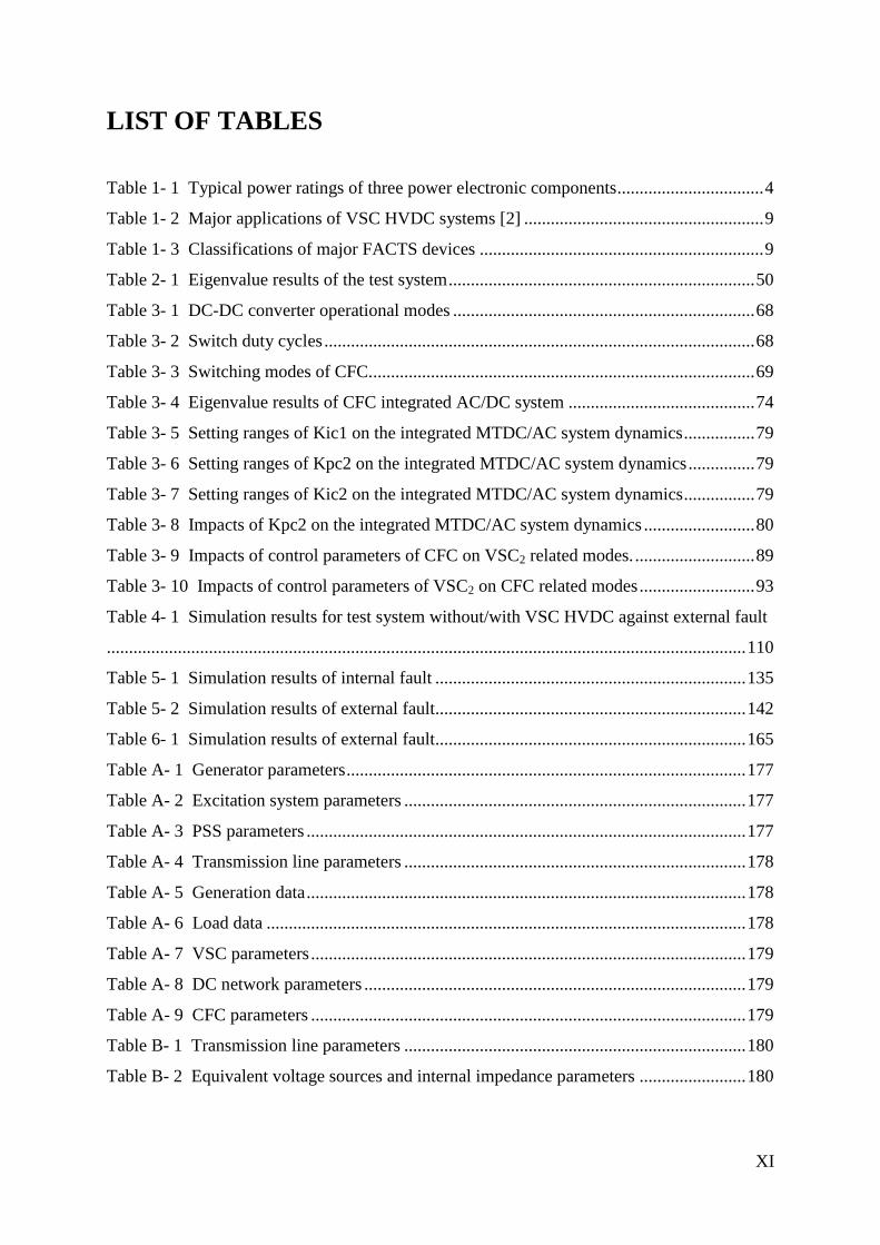
Table 1- 2 shows the major applications of VSC HVDC systems.

Table 1- 2 Major applications of VSC HVDC systems [2]

Project Country Year Topology Power DC Voltage

Hallsjon Sweden 1997 2-level 3 MW ± 10 kV

Gotland Sweden 1999 2-level 50 MW ± 80 kV

Eagle Pass USA 2000 3-level 36 MW ± 16 kV

Terranora Australia 2000 2-level 180 MW ± 80 kV

Cross Sound USA 2002 3-level 330 MW ± 150 kV

Estlink Finland 2006 2-level 350 MW ± 150 kV

Trans Bay Cable USA 2010 MMC 400 MW ± 200 kV

Zhoushan China 2014 MMC 1 GW ± 200 kV

DolWin3 Germany 2017 MMC 900 MW ± 320 kV

1.1.2 VSC FACTS

Along with the developments of VSC HVDC, VSC flexible alternating current system

(FACTS) also continue to advance in recent decades as a power electronic based system to

enhance power system controllability and increase power transfer capability [56-59]. On the

contrary to the conventional thyristor based reactive power compensator (such as SVC,

TCSC, and TCSR), VSC FACTS (such as STATCOM, SSSC and UPFC) are built upon self-

commutating controllable switches (such as GTO and IGBT) [60-63]. The FACTS systems

are applied to power systems for reactive power compensation, bus voltage regulation, power

flow control, power quality improvement, and system stability enhancement [64-66]. The

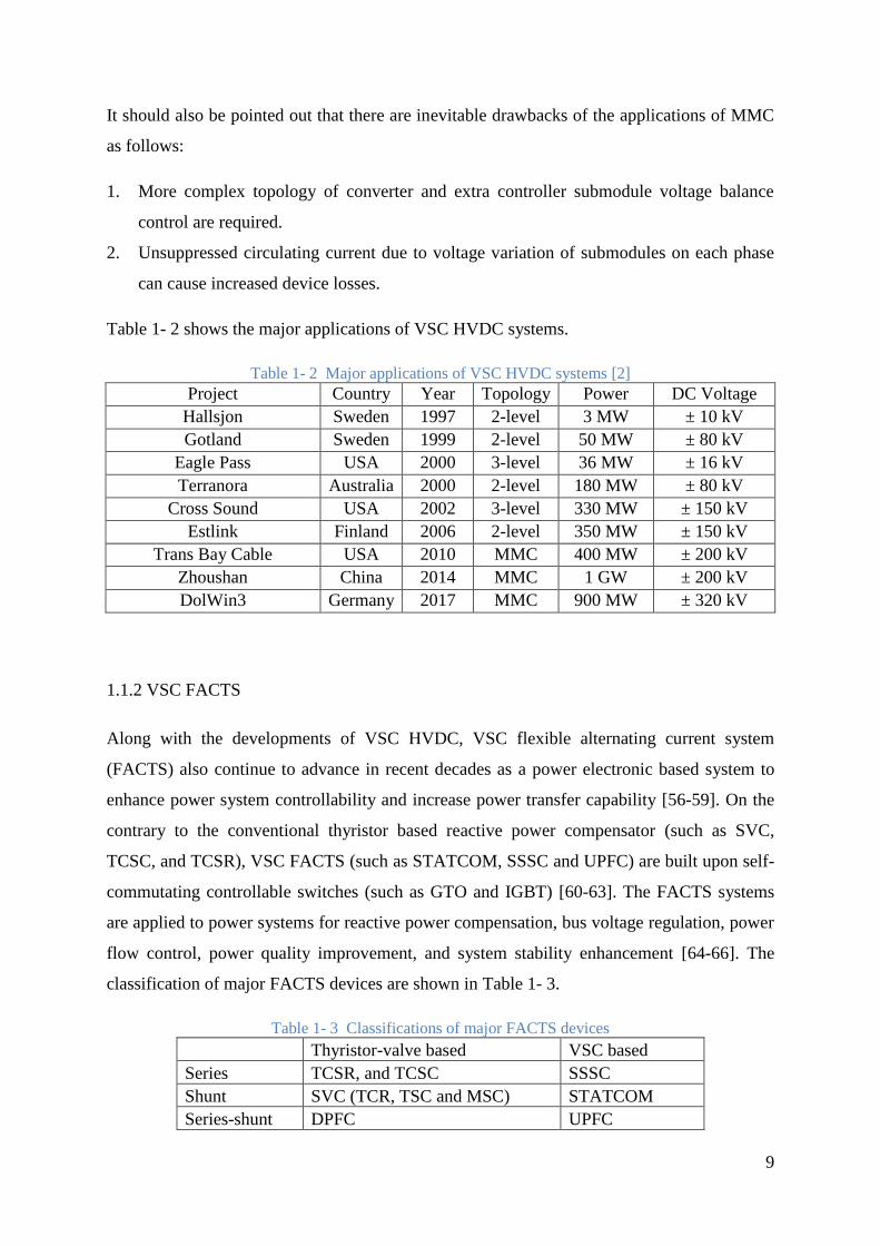
classification of major FACTS devices are shown in Table 1- 3.

Table 1- 3 Classifications of major FACTS devices

Thyristor-valve based VSC based

Series TCSR, and TCSC SSSC

Shunt SVC (TCR, TSC and MSC) STATCOM

Series-shunt DPFC UPFC

10

Static synchronous compensator (STATCOM) is a promising shunt connected FACTS, which

generates three-phase balanced output voltage at fundamental frequency with rapidly

controllable amplitude and phase angle [67-69]. STATCOM is used as a typical example of

shunt VSC FACTS to study stability, control and protection of VSC FACTS in this thesis. A

STATCOM can provide the connected power system with reactive power control or bus

voltage regulation support at PCC. The major advantages of STACOM compared to thyristor

based FACTS are quick response time, optimum voltage waveform, smaller footprint

requirement, and higher operational flexibility [60,70-71]. Figure 1- 10 shows a basic

configuration of a two-level star-connection STATCOM.

to AC System

+

-

DC side

Figure 1- 10 Configuration of a two-level star-connection STATCOM.

1.1.3 CFC in MTDC

The major established applications of HVDC interconnections are using two-terminal point-

to-point or back-to-back configuration [2]. However, with more and more installed and

planned applications of multi-terminal HVDC transmission systems, the current flow control

of DC grid has become a challenge [72-75].

In DC grids with no DC power flow control, the DC currents are flowing from one node to

another through the path of least resistance. This may result in the situation where one or

more DC branches are overloaded. In a multi-terminal VSC based DC grid, the DC voltage

level is usually regulated by one VSC converter station, whilst other converter stations

control active power of connected DC branch [76-80]. In this way, the DC power flow can be

controlled by VSC converter stations in a DC grid with a simple radial topology. However,

for a DC grid with more complex meshed topology, additional meshed DC transmission lines

11

or DC cables may be used. In consequence, such DC power flow control by use of only

converter stations is not feasible because the number of DC branch exceeds the number of

converter station. New DC power flow control methods or devices are required.

There are three approaches for controlling DC power flow as follows:

1. Variable Series Resistor.

2. Series Voltage Source.

3. DC-DC Converter.

The principle of controlling DC power flow by use of variable series resistor is to insert a

number of additional resistors in series with a DC transmission line. Each resistor is

controlled by mechanical or electronic based switch to be embedded into DC line in series or

to be bypassed. In this way, the total amount of additional resistance can be controlled by

switching on or switching off these switches. The impedance of DC network is changed by

insertion of variable series resistors and the DC power flow is changed in consequence.

The disadvantage of this approach is that the standing power losses due to the additional

resistance is significant compared with the overall cable losses [72-73,81-83]. And the cost of

additional cooling equipment is required for power electronic based switching devices.

The principle of controlling DC power flow by use of series voltage source is to insert

controlled voltage source in series with a DC line to vary the voltage in the embedded branch.

The DC power flow of series voltage source integrated can be controlled by controlling the

magnitude and polarity of inserted voltage source. The voltage source can be regarded as a

power sink (when it absorb power to the DC branch) or a power source (when it provide

power to the DC branch), depending on the polarity. The practical implementation of the

series voltage source is achieved by thyristor, or IGBT based AC/DC converter.

The disadvantage of this approach is the cost of these additional AC/DC converters and their

power losses [72-73,82]. And the power rating of the voltage source is relatively small

compared to the DC network.

As for controlling DC power flow by use of DC-DC converters, DC current flow controller

(CFC) is a DC-DC converter based device which can provide multi-line flexible current flow

control in a simple meshed DC network. Figure 1- 11 shows the topology of a two-line CFC.

By control of DC-DC converter, CFC is capable of controlling current flow of the connected

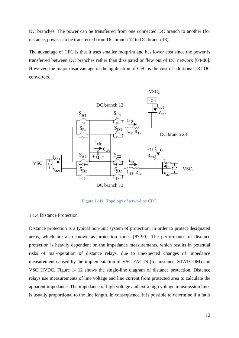
12

DC branches. The power can be transferred from one connected DC branch to another (for

instance, power can be transferred from DC branch 12 to DC branch 13).

The advantage of CFC is that it uses smaller footprint and has lower cost since the power is

transferred between DC branches rather than dissipated or flew out of DC network [84-86].

However, the major disadvantage of the application of CFC is the cost of additional DC-DC

converters.

�

�

�

� �

�

�

�

+ -

VSC1

VSC2

VSC3

icfc

DC branch 12

DC branch 13

DC branch 23

Figure 1- 11 Topology of a two-line CFC.

1.1.4 Distance Protection

Distance protection is a typical non-unit system of protection, in order to protect designated

areas, which are also known as protection zones [87-90]. The performance of distance

protection is heavily dependent on the impedance measurements, which results in potential

risks of mal-operation of distance relays, due to unexpected changes of impedance

measurement caused by the implementation of VSC FACTS (for instance, STATCOM) and

VSC HVDC. Figure 1- 12 shows the single-line diagram of distance protection. Distance

relays use measurements of line voltage and line current from protected area to calculate the

apparent impedance. The impedance of high voltage and extra high voltage transmission lines

is usually proportional to the line length. In consequence, it is possible to determine if a fault

13

occurs in the protection zone or out of protection zone by comparing the calculated

impedance to the protected line impedance [91-96].

Vsource

Zs Zlinea Zlineb

Distance

Relay

faultIrelay

Vrelay

Ifault

Figure 1- 12 Single-line diagram of distance protection.

Distance protection is considered to be simple to apply and fast in operation for faults located

along most of a protected circuit. It is suitable for application with high-speed auto-reclosing

[97-99]. The measured apparent impedance by distance relay is independent of the source

impedance.

Distance relays are designed to operate only when faults occurred are within the protection

zone, which is the protection range between the relay location and the selected reach point.

The calculated apparent impedance is compared with the reach point impedance. If the

calculated apparent impedance is less than the reach point impedance, it is assumed that a

fault occurred on the line between the relay and the reach point. The distance relay operates

and sends signals to related circuit breakers (CB) and circuit breakers trip. If the calculated

apparent impedance is greater than the reach point impedance, it is assumed that no fault

occurred on the line between the relay and the reach point. Once the settings of a distance

relay are determined, the protection is relatively unaffected by changes in the power systems

[100-101].

The reach point of a distance relay is a certain point along the line impedance locus which

indicates the boundary of protection. The reach point can be plotted on an R/X diagram since

it is dependent on the ratio of voltage and current and phase angle between them.

The major advantages of distance protection are as follows [87,92-93]:

1. High-speed of operation.

2. Ability to protect independent of communication services.

14

And the major disadvantages of distance protection are considered to be as follows [92-

93,95]:

1. Need of both CTs (current transformer) and VTs (voltage transformer).

2. Limited resistive fault coverage.

1.2 Literature Review

1.2.1 Modelling and Control of VSC HVDC and VSC FACTS

dq decoupled control, which is also known as vector control, is the most commonly used

control strategy of VSC converters, compared to the conventional “voltage margin method”

presented in [7] and the other control methods of output voltage magnitude and phase angle

used in [8,9,13,41]. VSC HVDC systems use dq decoupled control to achieve independent

control of active power and reactive power [102-103]. As dq decoupled control presented in

[10-11,17], active power or DC voltage is controlled in d axis, while reactive power or AC

voltage is controlled in q axis. Figure 1- 13 shows the architecture of a typical dq decoupled

control system. The advantage of using dq decoupled control is that the independent control

of active power or DC voltage in d axis and reactive power AC voltage can be achieved while

the conventional control of converter output voltage magnitude and phase angle can not. dq

decoupled control is also widely used for VSC HVDC system connections of offshore wind

farms and VSC FACTS compensation, as deeper penetration of distributed resources into

modern power systems [23,28,35]. Novel control strategies of VSC converters are also

emerged as alternatives to meet various control purposes such as power synchronization

control in [14-16,18] for avoidance of instability caused by a standard phase-locked loop in a

weak AC-system connection , and impedance based resonance control in [14] by use of

resonance stability analysis.

15

Σ+

-PI

Σ+

-PI Σ

PI

Σ+

-PI Σ

ωL

ωL

+

+

+

+

-

+

xSelector

DC voltage

regulation

active power

control

Σ+

-

xSelector

AC voltage

regulation

reactive power

control

converter outer control loop converter inner control loop

Figure 1- 13 Architecture of dq decoupled control.

For MMC based VSC HVDC systems, the major control strategies mentioned above can be

extended to application of MMC, since MMC is essentially a new topology of VSC. As two-

terminal back-to-back MMC HVDC system presented in [46] and two terminal point-to-point

MMC HVDC system presented in [49], dq decoupled control is applied. The general control

strategy of two-terminal VSC HVDC system (including MMC HVDC system) using dq

decoupled control is that one VSC terminal regulates DC voltage level and AC voltage at its

PCC while the other VSC terminal control active power transfer through the HVDC link and

AC voltage at its PCC [44]. The major difference of control systems between MMC and VSC

is that the control block of modulation of submodules is necessary for MMC.

For VSC MTDC systems, master-slave control [104] and voltage droop control [34,105-106]

are two major control strategies of VSC converters. For the master-slave control, one VSC

terminal operates as “master” to regulate DC voltage level of DC network, while the other

VSC terminals act as “slave” to control their active power transfer through VSC terminals.

For droop control, the control of DC voltage or active power are shared amount all VSC

terminals. The advantage of the master-slave control of VSC converters in VSC based MTDC

system as presented in [104,107-109], is relatively simple control design since additional

droop control loop is not used. However, the drawback of the master-slave control is that the

16

collapse of DC voltage level may occur, resulting from a severe fault occurred at the master

VSC terminal.

The master-slave control is used in this thesis for control of VSC based MTDC system. The

mathematical modelling of single VSC converter using dq decoupled control is presented in

[10-11,17,28], which considers the dynamic characteristic of control system of VSC, and

power transfer between AC system and DC network through VSC converter. The

mathematical modelling of VSC based MTDC system is presented in [24,26,35], which

considers the dynamic characteristic of VSC and DC network.

Static synchronous compensator (STATCOM), or static synchronous condenser (STATCON),

is a power electronics VSC based regulating device integrated to AC power transmission

system [58,61-62]. As the same with VSC HVDC system, there a number of various

topologies of STATCOM in different voltage levels, since the converter of STATCOM is

VSC based. These topologies vary in different voltage levels, depending on different

application scenarios: two-level converter, three-level converter, or multilevel modular

converter [110-112]. As for the connection topologies for converter legs, unlike VSC HVDC

system, there are two connections for converter legs of STATCOM, star-connection and

delta-connection. The topology of two-level star-connection STATCOM is shown in Figure

1- 10 while the topology of a MMC based delta-connection STATCOM is shown in Figure 1-

14.

17

26 submodules

Reactor Reactor

to AC System

Figure 1- 14 Configuration of a MMC-based delta-connection STATCOM.

The major control strategies of VSC converter can be extended to STATCOM, since

STATCOM is based on VSC converter technology. dq decoupled control is the most

commonly used control strategy of STATCOM, compared to conventional control strategies

based on 𝛼𝛽 control (which uses currents in 𝛼𝛽0 frame instead of dq0 frame as controlled

variables to generate converter output voltage) presented in [58,63,113]. As dq decoupled

control of STATCOM presented in [60,64-65,67-71,116-117]， AC side voltage at PCC or

the reactive power compensated by STATCOM is controlled by use of q axis current. And as

presented in [60,64-65,67-71,116-117], during normal steady state operation with the active

power loss of converter ignored, the generated voltage of STATCOM is in phase with voltage

at PCC of connected power system. This means there is no active power flow between

STATCOM and connected power system. Only reactive power is transferred. When 𝑄 is

positive, the STATCOM supplies reactive power to the external ac network. When 𝑄 is

negative, the STATCOM absorbs reactive power from the external ac network. The amount

of reactive power transfer during steady state can be expressed as follows:

𝑄 =𝑉𝑐,𝑎𝑏𝑐−𝑉𝑡,𝑎𝑏𝑐

𝑋𝑐𝑉𝑡,𝑎𝑏𝑐 (1. 1)

The advantage of using dq decoupled control is that the independent control of DC voltage in

d axis and reactive power/AC voltage in q axis can be achieved while the conventional

control of converter output voltage can not. This applies to the star-connection VSC based

STATCOM. For MMC based delta-connection STATCOM, normally only q axis current is

used to control reactive power or AC voltage, since there is no DC side energy storage

18

capacitor of STATCOM [69,115]. As dq decoupled control of delta-connection STATCOM

presented in [115] and other independent three-phase voltage control presented in [59,119-

120], the advantages of using delta-connection STATCOM are lower rated current of

switching devices and negative sequence current compensation in unbalanced circuit. MMC

converter has also been extended to the application of STATCOM due to its advantages of

increased voltage levels of output waveform and reduced switching losses caused by

switching frequency [69,121-125]. Control block of modulation of submodules should be

added into dq decoupled control of MMC based STATCOM [69].

dq decoupled control is used in this study for the control of delta-connection STATCOM.

The mathematical modelling of VSC converters using dq decoupled control is presented in

[60, 64-65,67-71,116-117], which considers the dynamic characteristic of control system of

STATCOM, DC voltage across DC energy storage capacitor, and reactive power transfer

between AC system and STATCOM.

1.2.2 Small-Signal Stability Analysis of VSC MTDC

With the increasing installations of VSC HVDC systems in power grids, the investigation of

controllability and stability of MTDC systems becomes important for it benefits the existing

AC systems with a means of increased energy trading between interconnected system

operators [126-127]. The generalized dynamic model of VSC MTDC is derived in a number

of papers, for instance [11-12,35,77-78,128-143], to investigate dynamic stability of VSC

MTDC in different scenarios. Various control strategies of MTDC system including the

master-slave DC voltage control, voltage and power droop control, and power

synchronization control are presented in [76-80,137,143-145]. Advanced control extensions

with distributed DC voltage control were developed in [137], and a supplementary

decentralized control structure to damp interarea oscillations was proposed in [76]. Frequency

support function for the surrounding interconnected AC systems and adaptive droop control

for effective power sharing through MTDC system were presented and analysed in depth in

[77,141]. Electromechanical transient modelling of MMC MTDC was studied in [146] to

provide the theoretical foundation for future MMC MTDC applications.

Small-signal stability analysis has been widely used for the study of system dynamics and

design of controllers for VSC [6,26,147-150]. For VSC-based MTDC system, small-signal

stability analysis is used to study if the MTDC system is capable of maintaining synchronism

19

(in broaden sense) when it is subjected to small disturbances [6,147]. Small-signal stability

analysis has been applied in [11,77-78,130-133,135-137,139-142,151-152] to study the

impacts of different control strategies, system parameters, and power system devices on

system dynamic stability. In [140] the small-signal stability analysis has been carried out for

a symmetric bipolar MTDC grid where different modes and interaction between AC systems

and VSC following various disturbances were characterized. In [139] small-signal stability

analysis was carried out to define the ranges for the gains of VSC controllers that ensure the

dynamic stability of MTDC system. Wind farm generators were considered and a method to

calculate converter controller gains was provided in [137]. In [141], an adaptive frequency

droop control was proposed by investigating the sensitivity of eigenvalues with respect to

different droop coefficients, control parameters and changes in operating conditions. In [77],

small-signal stability analysis was used for the design of an adaptive droop control scheme.

In [132], a method was introduced for systematically identifying interactions of modes in a

VSC MTDC system by analysing the participation pattern from different system elements.

Modal analysis is a commonly used approach in small-signal stability analysis to reflect

dynamic characteristic of studied systems. It can provide enlightening insights of the essential

dynamic behaviour of state variables by use of mathematical analysis of eigenvalue results.

Modal analysis is used as the approach to study dynamic response of VSC based MTDC

systems against small perturbation in [77,132-133,135, 139-142,151-153]. Eigenvalues of

state matrix can be calculated based on dynamic equations of MTDC system in state- space

representation, which consists of state variables and inputs. By analysing of the values of

eigenvalue results, the time dependent characteristics of modes can be determined, including

oscillation type, frequency of oscillation, and damping ratio [11,77,132-133,135, 139-

142,151-153].

Eigenvalue trajectory study is a means of modal analysis to reveal impacts of certain

parameter of power systems, or control system on eigenvalues [6,11,77,132-133,140,151-

153]. The trajectory of varying pole placements of eigenvalues is plotted on a complex plane

in response to the changing of certain studied parameter. Eigenvalue trajectory analysis is

used in [11,77,132-133,141,151-153] to investigate the impacts of control parameter, system

strength, short-circuit ratio, and phase locked loop (PLL) parameters on root locus of test

system for the purpose of control system design [11,77,141,153], interactions studies between

power system components[132-133,151], and coordination optimization of multi VSC

converters [141,152].

20

Previous publications on small-signal stability analysis of VSC MTDC have been focused on

the dynamics of VSC converters while there is a lack of consideration of DC networks with

CFC. Hence there is also a lack of analysis on the potential impacts of DC power flow

controller on existing MTDC system in terms of network stability and dynamic performance

under disturbances. There is a real need to fill in the gap of the interactions between DC

networks with CFC and VSC (even more broadly, the detailed representation of connected

AC networks).

1.2.3 Impacts of VSC HVDC and VSC FACTS on Distance Protection

The emerging shunt VSC FACTS (for instance, STATCOM) and VSC HVDC technology are

commonly regarded as effective solutions for fast-response voltage/reactive power support

during normal and faulty conditions [64,67]. In recent years, there has been an increase of

STATCOM applications and VSC HVDC integrations in the high voltage (HV) transmission

systems around the world [121].

However, the implementations of VSC FACTS and VSC HVDC in the HV transmission

systems may introduce certain risks to the existing protection and control (P&C) systems

[89,154]. For example, if one or more VSC FACTS (in particular, STATCOM as an example

studied in this thesis) or VSC converters are put into service for fast voltage/reactive power

control, it may cause unexpected transient changes of impedance [155]. As the performance

of feeder distance protection is heavily dependent on the impedance measurements, these

unexpected changes of impedance may trigger mal-operation of feeder distance protection.

As a result, such risk should be carefully investigated when introducing the VSC FACTS and

VSC HVDC into HV transmission system.

In [155], comparative investigation of the performance of various distance protection

schemes is presented for transmission lines compensated by shunt connected FACTS devices.

In [156], the impacts of VSC based multiline FACTS controllers on distance relays are

evaluated. An adaptive distance protection scheme in the presence of STATCOM is

presented in [157]. An adaptive distance protection scheme is proposed in [158] to improve

the performance of the conventional distance protection scheme for compensated lines with

high resistance faults. In [159], a methodology of calculation of fundamental frequency-based

per phase digital impedance pilot relaying scheme for STATCOM compensated transmission

lines is presented using two end synchronised measurements.

21

The study of the impacts of HVDC interconnectors on distance protection are mainly focused

on the measurement accuracy at the boundary of protection zones [160-161]. A fast full-line

tripping distance protection method for HVDC transmission line is proposed in [160] to

achieve accurate measurement near protection zone boundary to distinguish internal faults

from external faults. The representation of HVDC transmission line is in distributed

parameter model to design tripping distance protection method. In [161], the application of

distance protection for HVDC transmission lines is considered in frequency-dependent

parameter model to enhance the calculation accuracy of fault distance. However, these

studies are on distance protection design for DC cable of conventional LCC HVDC link. The

impacts of VSC HVDC systems on distance protection are yet to be investigated.

The methodologies of the study of STATCOM’s impacts on feeder distance protection can be

extended to the study of impacts of VSC HVDC systems on distance protection, since

STATCOM and VSC HVDC are both VSC converter based, and the commonly used control

strategies of them are same dq decoupled control. In [162], a robust distance protection

approach is proposed to consider these impacts based on 𝜇 synthesis analysis. The apparent

impedance measurements of distance relays affected by infeed current from VSC HVDC

connected bus are studied in [163-165]. An apparent impedance calculation method

considering impacts of VSC HVDC is presented in [164] to identify the possible mal-

operations of distance relays in aspects of Zone 2 protection. It should also be noted that the

potential interactions between VSC HVDC and STATCOM are analysed in [166-167] to

provide some insights of approaches to investigate their interactions.

The major research gaps can be concluded as follows:

1. The previous research on small-signal stability analysis of VSC MTDC have been

focused on the dynamics of VSC converters while there is a lack of consideration of DC

networks.

2. There is also a lack of studies on the potential impacts of DC power flow controllers on

existing MTDC systems in terms of network stability and dynamic performance under

disturbances.

3. The previous research on distance protection considering the effects of VSC FACTS are

mainly on impacts of SVC or STATCOM only while there has no studies on the

combined impacts of VSC FACTS and VSC HVDC under various fault scenarios.

22

1.3 Research Focuses and Contributions

1.3.1 Research Focuses

The main research focuses of this thesis are:

1. To implement detailed mathematical models of integrated AC/DC system consisting

multiple AC synchronous generators, VSC, and CFC.

2. To use modal analysis to characterize modes, via participation factor matrix, of the

integrated AC/DC systems without/with CFC and hence investigate the impacts of CFC

on the integrated AC/DC system.

3. To validate the small-signal stability analysis results in RTDS by simulating small and

large disturbances.

4. To investigate the effects of the control parameters of CFC controller on system stability

and interactions between CFC and VSC.

5. To derive the mathematical representations of the apparent impedance measurements of

feeder distance relays considering the current infeed from VSC HVDC and VSC FACTS

at difference locations.

6. To study the impacts of VSC HVDC and VSC FACTS on distance protections, and

validate the results by dynamic simulations in hardware in the loop (HIL) RTDS

platform against various fault scenarios.

1.3.2 Scientific Contributions of the Thesis

The main contributions of the work presented in this thesis to fill aforementioned research

gaps are summarized as follows:

1. A small-signal stability model of integrated AC/DC systems with VSC and CFC to

characterize modes via participation factor matrix and investigate various control

parameters on the eigenvalue trajectories of system modes.

2. The investigation of the interactions between CFC and VSC including impacts of control

parameters of CFC on VSC and impacts of control parameters of VSC on CFC.

3. The mathematical representations of the apparent impedance measurements of feeder

distance relays against various fault scenarios considering the current infeed from VSC

HVDC and VSC FACTS at difference locations.

23

1.4 Outline of the Thesis

The thesis is presented based on both theoretical analysis and time domain simulations in

RTDS. The thesis is organized as follows:

Chapter 2: The multi-model system in state-space representation is derived, including

synchronous generators with excitation system and power system stabiliser (PSS), network

power flow equations, VSC with its control system, and DC network without CFC. The

small-signal stability analysis of VSC based MTDC system without CFC is implemented and

validated in time domain simulations in RTDS.

Chapter 3: The modelling of DC network with CFC in state-space representation is derived,

linearized, and merged into the VSC based MTDC system without CFC presented in Chapter

2 to formulate multi-model system with CFC. The small-signal stability analysis of VSC

based MTDC system with CFC is implemented and validated in time domain simulations in

RTDS to investigate interactions between CFC and VSC. The interactions between VSC and

CFC are investigated by use of eigenvalue trajectory studies.

Chapter 4: The mathematical representation of the apparent impedance measurements of

distance relays is derived considering the infeed current from VSC HVDC. Relevant analysis

of the apparent impedance measurement representation and dynamic simulation study is

performed to investigate the impacts of VSC HVDC systems on distance protection.

Chapter 5: The modelling of MMC based delta-connection STATCOM is presented,

including configuration and control system. The mathematical representation of the apparent

impedance measurements of distance relays is derived considering the infeed current from

VSC FACTS connected busbar. Relevant analysis of the apparent impedance measurement

representation and dynamic simulation study is performed to investigate the impacts of VSC

FACTS on distance protection.

Chapter 6: The mathematical representation of the apparent impedance measurements of

distance relays is derived considering the infeed currents from both VSC HVDC and shunt

VSC FACTS at different locations. Relevant analysis of the apparent impedance

measurement representation and dynamic simulation study is performed to investigate the

impacts of VSC HVDC and VSC FACTS on distance protection.

24

Chapter 7: This chapter concludes the thesis and list possible promising future works that

could be done.

The thesis can be divided into four parts as follows, to illustrate the overall structure:

1. Part 1, i.e. Chapter 1, presents the research background, literature review, research

contributions, and outline of the thesis

2. Part 2 consists of Chapter 2 and Chapter 3, which study small-signal stability of VSC

MTDC system. The small-signal stability analysis of VSC MTDC system without CFC is

conducted in Chapter 2. Based on achievements in Chapter 2, Chapter 3 incorporates CFC

into the VSC MTDC system established in Chapter 2 and investigates the interactions

between VSC and CFC by use of modal analysis in Chapter 3.

3. Part 3 consists of Chapter 4, Chapter 5, and Chapter 6, which study the impacts of VSC

HVDC and VSC FACTS on existing distance protection. Chapter 4 investigates the

impacts of VSC HVDC on distance protection. Chapter 5 investigates the impacts of VSC

FACTS on distance protection. Chapter 6 considers VSC HVDC and multiple VSC

FACTS integrated to system simultaneously and their corporate impacts on distance

protection under different fault scenarios.

4. Part 4, i.e. Chapter 7, presents the conclusions and future work of the thesis.

Part 2 and Part 3 present the major technical contributions of the thesis, which present the

impacts of the integration of VSC HVDC and VSC FACTS on dynamic stability and

protection issues of connected systems.

25

CHAPTER 2 SMALL-SIGNAL STABILITY ANALYSIS

OF VSC BASED MTDC SYSTEM WITHOUT DC CFC

2.1 Introduction

This chapter presents the dynamic modelling of the integrated MTDC/AC system without

integration of CFC to study the small-signal stability of VSC-based MTDC system. In 2.2,

the modelling of AC power system is presented in dynamic equations, including synchronous

generator with excitation system and PSS. The network power flow equations are also

presented to reflect mathematical relationships between busbars of AC network in algebraic

equations. In 2.3, the modelling of MTDC system without CFC is presented in dynamic

equations, including VSC with its control system and generalized DC network without CFC.

Multiple VSC converters are applied to link meshed DC network and AC systems.

Aggregated parameter model of R-L based DC transmission lines is considered for the

representation of DC network. In 2.4, AC power system and MTDC system without CFC are

linearized around equilibrium point to derive their small-signal state-space model of

subsystems. Then the state-space models of subsystems of AC power system and MTDC

system are formulated by substitution of the network power flow algebraic equations. In 2.5,

a test system that consists of multiple synchronous generators with excitation system and PSS,

multiple VSC converters, and DC network without CFC, is established to study its small-

signal stability. Small-signal model of test system is derived based on sub-models from 2.2-

2.4 and the eigenvalues of state-space representation of the test system are calculated. Modal

analysis of the eigenvalues results is performed to study small-signal stability of VSC based

MTDC system without CFC. In 2.6, simulations results of established AC/DC system against

small disturbances and large disturbances (including AC system faults, and DC cable faults)

in RTDS/RSCAD are analysed to validate modal analysis results.

2.2 Modelling of AC Power System

VSC HVDC systems and VSC-based MTDC systems are applied to power systems for bulk

power transmission. The AC power system dynamics are modelled in aspects of two major

parts: synchronous generators (including excitation system and PSS) and the power network.

26

2.2.1 Synchronous Generator with Excitation System and PSS

Synchronous generators are still the majority source of commercial electrical energy [6].

They are commonly used in power generation to convert mechanical power into electrical

power for the grid. There has been a significant number of literature on synchronous

machines in a variety of complexity levels from second-order classic swing model to a

detailed model in the order of up to eight [6, 148-150]. A 6th

-order generator model is

selected in this thesis so that the modelling of the synchronous generator is considered to be

sufficient to reflect the transient and sub-transient dynamic characteristic of synchronous

machines [149]. The state variables 𝒙𝒊 of the 6th

-order generator model are as follows:

xi = [δi, ωi, Eqi′ , E i

′ , φ i, φ qi]T (2. 1)

for i = 1, 2, …, m, where

i : index number of synchronous generator

m : total number of synchronous generators

𝛿𝑖 : rotor angle of synchronous generator

𝜔𝑖 : rotor angular velocity of synchronous generator

𝐸𝑞𝑖′ : transient electromagnetic force caused by field flux linkage in q-axis

𝐸𝑑𝑖′ : transient electromagnetic force caused by field flux linkage in d-axis

𝜑 𝑑𝑖 : subtransient electromagnetic force caused by field flux linkage in d-axis

𝜑 𝑞𝑖 : subtransient electromagnetic force caused by field flux linkage in q-axis

Then the differential equations representing the subtransient dynamic behaviour of the

synchronous generators i is given by:

δi̇ = ωi − ωs (2. 2)

�̇�𝑖 = 1

𝑀𝑖[𝑇𝑀𝑖 − 𝐷𝑖(𝜔𝑖 − 𝜔𝑠) + (𝑋𝑑𝑖

′′ − 𝑋𝑞𝑖′′ )𝐼𝑑𝑖𝐼𝑞𝑖 −

(𝑋𝑑𝑖′′ − 𝑋𝐿𝑖)

(𝑋𝑑𝑖′ − 𝑋𝐿𝑖)

𝐼𝑞𝑖𝐸𝑞𝑖′ −

(𝑋𝑑𝑖′ − 𝑋𝑑𝑖

′′ )


𝐼𝑞𝑖𝜑 𝑑𝑖

27

−(𝑋𝑞𝑖

′′−𝑋𝐿𝑖)

(𝑋𝑞𝑖′ −𝑋𝐿𝑖)

𝐼𝑑𝑖𝐸𝑑𝑖′ +

(𝑋𝑞𝑖′ −𝑋𝑞𝑖

′′)


𝐼𝑑𝑖𝜑 𝑞𝑖 ] (2. 3)

�̇�𝑞𝑖′ =

𝑇𝑑𝑜𝑖′ [−𝐸𝑞𝑖

′ + (𝑋𝑑𝑖 − 𝑋𝑑𝑖′ )(𝐼𝑑𝑖 −

(𝑋𝑑𝑖′ −𝑋𝑑𝑖

′′)

(𝑋𝑑𝑖′ −𝑋𝐿𝑖)

2 [𝜑 𝑑𝑖 + (𝑋𝑑𝑖′ − 𝑋𝐿𝑖)𝐼𝑑𝑖 − 𝐸𝑞𝑖

′ ] + 𝐸𝑓𝑑𝑖)] (2. 4)

�̇�𝑑𝑖′ =

𝑇𝑞𝑜𝑖′ [−𝐸𝑑𝑖

′ + (𝑋𝑞𝑖 − 𝑋𝑞𝑖′ )(𝐼𝑞𝑖 −


′′)


2 [𝜑 𝑞𝑖 + (𝑋𝑞𝑖′ − 𝑋𝐿𝑖)𝐼𝑞𝑖 + 𝐸𝑑𝑖

′ ])] (2. 5)

�̇� 𝑑𝑖 =

𝑇𝑑𝑜𝑖′′ [−𝜑 𝑑𝑖 + 𝐸𝑞𝑖

′ − (𝑋𝑑𝑖′ − 𝑋𝐿𝑖)𝐼𝑑𝑖] (2. 6)

�̇� 𝑞𝑖 =

𝑇𝑞𝑜𝑖′′ [−𝜑 𝑞𝑖 − 𝐸𝑑𝑖

′ − (𝑋𝑞𝑖′ − 𝑋𝐿𝑖)𝐼𝑞𝑖] (2. 7)


𝜔𝑠 : rated rotor angular velocity of synchronous generator

𝑀𝑖 : shaft inertial constant of synchronous generator

𝐷𝑖 : synchronous mechanical damping constant of synchronous generator

𝑇𝑀𝑖 : mechanical torque input

𝑇𝑑𝑜𝑖′ , 𝑇𝑑𝑜𝑖

′′ : open circuit transient and subtransient time constant in d-axis, respectively

𝑇𝑞𝑜𝑖′ , 𝑇𝑞𝑜𝑖

′′ : open circuit transient and subtransient time constant in q-axis, respectively

𝑋𝐿𝑖 : armature leakage reactance

𝑋𝑑𝑖, 𝑋𝑑𝑖′ , 𝑋𝑑𝑖

′′ : synchronous, transient and subtransient reactance in d-axis, respectively

𝑋𝑞𝑖, 𝑋𝑞𝑖′ , 𝑋𝑞𝑖

′′ : synchronous, transient and subtransient reactance in q-axis, respectively

𝐸𝑓𝑑𝑖 : field voltage

𝐼𝑑𝑖 : stator current in d-axis

𝐼𝑞𝑖 : stator current in q-axis

For stability studies, the dynamics of synchronous generator terminal voltage is much slower,

compared to the dynamics of stator. Hence, the representation of synchronous generator

28

terminal voltage is given in algebraic equations rather than state equations. The algebraic

equations of generator terminal voltage are as follows:

𝑉𝑖 s n(𝛿𝑖 − 𝜃𝑖) −(𝑋𝑞𝑖



𝐸𝑑𝑖′ +


′′)


𝜑 𝑞𝑖 + 𝑅𝑠𝑖𝐼𝑑𝑖 − 𝑋𝑞𝑖′′ 𝐼𝑞𝑖 = 0 (2. 8)

𝑉𝑖 cos(𝛿𝑖 − 𝜃𝑖) −(𝑋𝑑𝑖



𝐸𝑞𝑖′ +


′′)


𝜑 𝑑𝑖 + 𝑅𝑠𝑖𝐼𝑞𝑖 + 𝑋𝑑𝑖′′ 𝐼𝑑𝑖 = 0 (2. 9)


𝑉𝑖 : magnitude of synchronous generator terminal voltage

𝜃𝑖 : phase angle of synchronous generator terminal voltage

𝑅𝑠𝑖 ∶ armature resistance

It should be noted that the synchronous generator terminal voltage (𝑉𝑖∠𝜃𝑖 for i = 1, 2, …, m, )

is the internal bus voltages of the generator connected buses. The same notations for the bus

voltages of non-generator buses are used as the generator buses, with i = m+1, m+2, …, n,

where n is the total number of buses of power network.

Then the dynamics of excitation system is considered and included as extension of the

modelling of synchronous generator. Static AC excitation system is used for synchronous

generators. The dynamics of excitation system is presented in differential equation as follows:

�̇�𝑓𝑑𝑖 = −

𝑇𝐴𝑖𝐸𝑓𝑑𝑖 +

𝐾𝐴𝑖

𝑇𝐴𝑖(𝑉𝑟𝑒𝑓𝑖 − 𝑉𝑖) (2. 10)


𝑉𝑟𝑒𝑓𝑖 : voltage reference of the excitation system

𝑇𝐴𝑖 : time constant of the voltage regulator

𝐾𝐴𝑖 : transient gain of the voltage regulator

Power system stabiliser (PSS) is commonly used with synchronous generator to add damping

to generator rotor oscillations by use of auxiliary stabilizing signals to control excitation

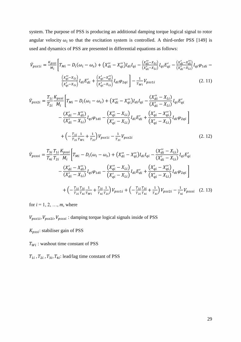
29

system. The purpose of PSS is producing an additional damping torque logical signal to rotor

angular velocity 𝜔𝑖 so that the excitation system is controlled. A third-order PSS [149] is

used and dynamics of PSS are presented in differential equations as follows:

�̇�𝑝𝑠𝑠 𝑖 =𝐾𝑝𝑠𝑠𝑖



(𝑋𝑑𝑖′′−𝑋𝐿𝑖)


𝐼𝑞𝑖𝐸𝑞𝑖′ −


′′)


𝐼𝑞𝑖𝜑 𝑑𝑖 −

(𝑋𝑞𝑖′′−𝑋𝐿𝑖)




′′)


𝐼𝑑𝑖𝜑 𝑞𝑖 ] −

𝑇𝑊𝑖𝑉𝑝𝑠𝑠 𝑖 (2. 11)

�̇�𝑝𝑠𝑠 𝑖 =𝑇 𝑖

𝑇 𝑖

𝐾𝑝𝑠𝑠𝑖





𝐼𝑞𝑖𝐸𝑞𝑖′

−(𝑋𝑑𝑖

′ − 𝑋𝑑𝑖′′ )


𝐼𝑞𝑖𝜑 𝑑𝑖 −(𝑋𝑞𝑖

′′ − 𝑋𝐿𝑖)

(𝑋𝑞𝑖′ − 𝑋𝐿𝑖)


(𝑋𝑞𝑖′ − 𝑋𝑞𝑖

′′ )


𝐼𝑑𝑖𝜑 𝑞𝑖 ]

+(−𝑇1𝑖

𝑇2𝑖

𝑇𝑊𝑖+

𝑇2𝑖)𝑉𝑝𝑠𝑠 𝑖 −

𝑇2𝑖𝑉𝑝𝑠𝑠 𝑖 (2. 12)

�̇�𝑝𝑠𝑠𝑠𝑖 =𝑇 𝑖

𝑇4𝑖

𝑇 𝑖

𝑇 𝑖

𝐾𝑝𝑠𝑠𝑖





𝐼𝑞𝑖𝐸𝑞𝑖′

−(𝑋𝑑𝑖

′ − 𝑋𝑑𝑖′′ )


𝐼𝑞𝑖𝜑 𝑑𝑖 −(𝑋𝑞𝑖

′′ − 𝑋𝐿𝑖)



(𝑋𝑞𝑖′ − 𝑋𝑞𝑖

′′ )


𝐼𝑑𝑖𝜑 𝑞𝑖 ]

+(−𝑇1𝑖

𝑇2𝑖

𝑇3𝑖

𝑇4𝑖

𝑇𝑊𝑖+

𝑇3𝑖

𝑇4𝑖

𝑇2𝑖)𝑉𝑝𝑠𝑠 𝑖 + (−

𝑇1𝑖

𝑇2𝑖

𝑇3𝑖

𝑇4𝑖+

𝑇4𝑖)𝑉𝑝𝑠𝑠 𝑖 −

𝑇4𝑖𝑉𝑝𝑠𝑠𝑠𝑖 (2. 13)


𝑉𝑝𝑠𝑠 𝑖, 𝑉𝑝𝑠𝑠 𝑖, 𝑉𝑝𝑠𝑠𝑠𝑖 : damping torque logical signals inside of PSS

𝐾𝑝𝑠𝑠𝑖: stabiliser gain of PSS

𝑇𝑊𝑖 : washout time constant of PSS

𝑇 𝑖 , 𝑇 𝑖 , 𝑇 𝑖 , 𝑇4𝑖: lead/lag time constant of PSS

30

2.2.2 Network Power Flow

The power-balance form of network power flow equations is used in this study. The network

power flow equations of active and reactive power flow for generator buses (PV buses) are in

algebraic equations as follows:

𝑉𝑖(𝐼𝑞𝑖 cos(𝛿𝑖 − 𝜃𝑖) + 𝐼𝑑𝑖 s n(𝛿𝑖 − 𝜃𝑖)) + 𝑃𝐿𝑖

= ∑ 𝑉𝑖𝑉𝑘(𝐺𝑖𝑘 cos(𝜃𝑖 − 𝜃𝑘) + 𝐵𝑖𝑘 s n(𝜃𝑖 − 𝜃𝑘))𝑛𝑘= (2. 14)

𝑉𝑖(𝐼𝑑𝑖 cos(𝛿𝑖 − 𝜃𝑖) − 𝐼𝑞𝑖 s n(𝛿𝑖 − 𝜃𝑖)) + 𝑄𝐿𝑖

= ∑ 𝑉𝑖𝑉𝑘(𝐺𝑖𝑘 s n(𝜃𝑖 − 𝜃𝑘) + 𝐵𝑖𝑘 cos(𝜃𝑖 − 𝜃𝑘))𝑛𝑘= (2. 15)


m : total number of generator buses

n : total number of buses of power network

𝐺𝑖𝑘 : conductance between bus i and bus k from admittance matrix

𝐵𝑖𝑘 : susceptance between bus i and bus k from admittance matrix

𝑃𝐿𝑖 : active power of loads on bus i

𝑄𝐿𝑖 : reactive power of loads on bus i

The network power flow equations of active and reactive power flow for non-generator buses

(PQ buses) are in algebraic equations as follows:

𝑃𝐿𝑖 = ∑ 𝑉𝑖𝑉𝑘(𝐺𝑖𝑘 cos(𝜃𝑖 − 𝜃𝑘) + 𝐵𝑖𝑘 s n(𝜃𝑖 − 𝜃𝑘))𝑛𝑘= (2. 16)

𝑄𝐿𝑖 = ∑ 𝑉𝑖𝑉𝑘(𝐺𝑖𝑘 s n(𝜃𝑖 − 𝜃𝑘) + 𝐵𝑖𝑘 cos(𝜃𝑖 − 𝜃𝑘)) 𝑛𝑘= (2. 17)

for i = m+1, m+2, …, n

31

2.3 Modelling of MTDC System without CFC

The MTDC system consists of multiple VSC converters and DC network. The topology,

control system and modelling of VSC are presented in 2.3.1. The DC network is formed of

DC transmission lines which are modelled by series resistors and inductors in 2.3.2. The DC

CFC is not included in this chapter but is to be studied in Chapter 3.

2.3.1 VSC with Its Control System

VSC is a fully controlled semiconductor based power converter. It uses self-commuted

semiconductor (for instance, IGBT) which can be turned on and turned off without relying on

line voltage. VSC is able to control active and reactive power independently.

There are a variety of topologies of VSC in different voltage levels, depending on different

application scenarios: two-level converter, three-level converter, or multilevel modular

converter. The typical topology of a two-level three-phase VSC is shown in Figure 2- 1. The

IGBT with antiparallel diode is used to form a valve. The DC bus capacitors C store energy

and filter DC harmonics. LC indicates the inductance of series AC reactor and coupling

transformer. RC indicates the equivalent resistance of reactor and power losses of converter.

The control system of VSC is realised by the control of turned on or turned off state of all six

valves. There is one valve in every arm of all six arms. There are two arms in each phase of

converter. There is always one valve turned on while the other one valve in the same phase

turned off. Hence the voltage at AC side of converter equals to either the positive or the

negative voltage of DC bus capacitor. The VSC converter applied in this study is two-level

converter.


+

-

Lc Rc

C

C

Figure 2- 1 Topology of a two-level three-phase VSC.

32

The single-line diagram (SLD) of a two-level VSC and its control system is shown in Figure

2- 2. dq decoupling control is used to regulate voltage at DC side Vdc or active power transfer

P in d frame and voltage at AC side VC,abc or reactive power transfer in q frame.

PWM and Pulse

Generator

abcdq0

PLL

abcdq0

θ

Vt,abc

Lc Rc

Vc,abcC

Vdc

Idc

abcdq0

Converter

Control System

Vt,dqVcref,dq

Vcref,abc

PCC

or or

C

Figure 2- 2 Single-line diagram of a two-level VSC and its control system.

The dq0 transformation (which is also known as the Park transformation) is usually used in

dq decoupling control for VSC. This method was firstly used in the modelling of

synchronous machines to reduce considerable complexity in solving synchronous machine

and power system problems and then spread to control strategy of VSC. It is an effective

approach to derive a simpler and clearer representation of the dynamics of VSC. The

transformation from the state variables in abc phase to dq0 variables is presented in the

following matrix form [6]:

[

𝑖𝑑𝑖𝑞𝑖0

] =

[ cos 𝜃 cos (𝜃 −

𝜋

) cos (𝜃 +

𝜋

)

− s n 𝜃 − s n (𝜃 − 𝜋

) − s n (𝜃 +

𝜋

)

]

[𝑖𝑎𝑖𝑏𝑖𝑐

] (2. 18)

where

𝑖𝑑 , 𝑖𝑞 , and 𝑖0 : state variables of currents in dq0 frame

𝑖𝑎 , 𝑖𝑏 , and 𝑖𝑐 : state variables of currents in abc phase

33

𝜃 : initial phase angle of d frame

The inverse transformation is presented as follows:

[

𝑖𝑎𝑖𝑏𝑖𝑐

] = [

cos 𝜃 −s n 𝜃 1

cos (𝜃 − 𝜋

) − s n (𝜃 −

𝜋

) 1

cos (𝜃 + 𝜋

) − s n (𝜃 +

𝜋

) 1

] [

𝑖𝑑𝑖𝑞𝑖0

] (2. 19)

The peak value of 𝑖𝑑 equals to the peak value of 𝑖𝑎. Under balanced condition 𝑖0 = 𝑖𝑎 + 𝑖𝑏 +

𝑖𝑐 = 0.

As the single-line diagram of the control system of VSC shown in Figure 2- 2, the line-to-line

voltages 𝑣𝑡,𝑎𝑏𝑐 and currents 𝑖𝑡,𝑎𝑏𝑐 at PCC (the primary side of the coupling transformer of

VSC) in abc phase, and DC current through one DC transmission line 𝐼𝑑𝑐 and DC voltage

across one DC energy storage capacitor 𝑉𝑑𝑐 at DC side of VSC are acquired. The line-to-line

voltages at PCC 𝑣𝑡,𝑎𝑏𝑐 is inputted into PLL block to compute its frequency f and phase angle

θ. Then the computed phase angle θ, along with line-to-line voltages 𝑣𝑡,𝑎𝑏𝑐 and currents 𝑖𝑡,𝑎𝑏𝑐

at PCC are input into two abc-to-dq0 transformation blocks to compute line-to-line voltages

𝑣𝑡,𝑑𝑞 and currents 𝑖𝑡,𝑑𝑞 in dq0 frame. The computed line-to-line voltages 𝑣𝑡,𝑑𝑞 and currents

𝑖𝑡,𝑑𝑞 in dq0 frame, along with acquired DC current 𝐼𝑑𝑐 , DC voltage 𝑉𝑑𝑐 , reference of DC

voltage 𝑉𝑑𝑐 ∗ or reference of active power transfer 𝑃∗, and reference of AC voltage at the AC

terminal of VSC 𝑉𝑎𝑐 ∗ or reference of reactive power transfer 𝑄∗ (these four references are set

by user) are inputted into the converter control system (which includes converter outer

control loop and converter inner control loop). Through converter control system block, the

output signal is computed, which is the reference of AC voltage at the AC terminal of

VSC 𝑣𝑐𝑟𝑒𝑓,𝑑𝑞in dq frame. Then the computed reference of AC voltage at the AC terminal of

VSC 𝑣𝑐𝑟𝑒𝑓,𝑑𝑞 is inputted dq0-to-abc transformation block. Through dq0-to-abc

transformation block, the output signal is the computed reference of AC voltage at the AC

terminal of VSC 𝑣𝑐𝑟𝑒𝑓,𝑎𝑏𝑐 in abc phase. The computed reference of AC voltage at the AC

terminal of VSC 𝑣𝑐𝑟𝑒𝑓,𝑎𝑏𝑐 is inputted into PWM and pulse generator block to compute PWM

signal and generate corresponding gate pulses to control valves of VSC. The output of PWM

and pulse generator block is gate pulse signals which are inputted into VSC to control every

valves of VSC to either turn on or turn off.

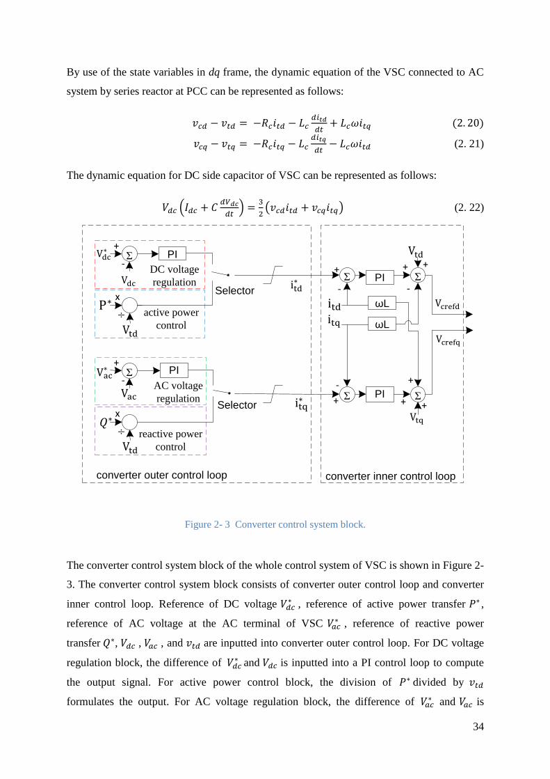
34

By use of the state variables in dq frame, the dynamic equation of the VSC connected to AC

system by series reactor at PCC can be represented as follows:

𝑣𝑐𝑑 − 𝑣𝑡𝑑 = −𝑅𝑐𝑖𝑡𝑑 − 𝐿𝑐𝑑𝑖𝑡𝑑

𝑑𝑡+ 𝐿𝑐𝜔𝑖𝑡𝑞 (2. 20)

𝑣𝑐𝑞 − 𝑣𝑡𝑞 = −𝑅𝑐𝑖𝑡𝑞 − 𝐿𝑐𝑑𝑖𝑡𝑞

𝑑𝑡− 𝐿𝑐𝜔𝑖𝑡𝑑 (2. 21)

The dynamic equation for DC side capacitor of VSC can be represented as follows:

𝑉𝑑𝑐 (𝐼𝑑𝑐 + 𝐶𝑑𝑉𝑑𝑐

𝑑𝑡) =

(𝑣𝑐𝑑𝑖𝑡𝑑 + 𝑣𝑐𝑞𝑖𝑡𝑞) (2. 22)

Σ+

-PI

Σ+

-PI Σ

PI

Σ+

-PI Σ

ωL

ωL

+

+

+

+

-

+

xSelector

DC voltage

regulation

active power

control

Σ+

-

xSelector

AC voltage

regulation

reactive power

control


Figure 2- 3 Converter control system block.

The converter control system block of the whole control system of VSC is shown in Figure 2-

3. The converter control system block consists of converter outer control loop and converter

inner control loop. Reference of DC voltage 𝑉𝑑𝑐 ∗ , reference of active power transfer 𝑃∗ ,

reference of AC voltage at the AC terminal of VSC 𝑉𝑎𝑐 ∗ , reference of reactive power

transfer 𝑄∗, 𝑉𝑑𝑐 , 𝑉𝑎𝑐 , and 𝑣𝑡𝑑 are inputted into converter outer control loop. For DC voltage

regulation block, the difference of 𝑉𝑑𝑐 ∗ and 𝑉𝑑𝑐 is inputted into a PI control loop to compute

the output signal. For active power control block, the division of 𝑃∗ divided by 𝑣𝑡𝑑

formulates the output. For AC voltage regulation block, the difference of 𝑉𝑎𝑐 ∗ and 𝑉𝑎𝑐 is

35

inputted into a PI control loop to compute the output signal. For reactive power control block,

the division of 𝑄∗divided by 𝑣𝑡𝑑 formulates the output. A selector is controlled by user to

assign the control system of VSC to operate either in DC voltage regulation or active power

control mode in d frame. Another selector is controlled by user to assign the control system

of VSC to operate either in AC voltage regulation or reactive power control mode in q frame.

The outputs of two selector blocks are then inputted to two limitation block to compute the

final output signals of converter outer control loop 𝑖𝑡𝑑∗ and 𝑖𝑡𝑞

∗ , which are the reference of

line-to-line current at PCC in dq frame.

When converter outer control loop operates in DC voltage regulation mode in d frame, the

current reference 𝑖𝑡𝑑∗ can be obtained from the converter outer control loop by:

𝑖𝑡𝑑∗ = 𝑘𝑝𝑑𝑐(𝑉𝑑𝑐

∗ − 𝑉𝑑𝑐) + 𝑘𝑖𝑑𝑐 ∫(𝑉𝑑𝑐∗ − 𝑉𝑑𝑐)𝑑𝑡

= 𝑘𝑝𝑑𝑐(𝑉𝑑𝑐∗ − 𝑉𝑑𝑐) + 𝑘𝑖𝑑𝑐𝑥 (2. 23)

where

𝑘𝑝𝑑𝑐 : proportional gain of the PI control loop of converter outer control loop in d frame

𝑘𝑖𝑑𝑐 : integral gain of PI control loop of converter outer control loop in d frame

𝑥 : auxiliary state variable to represent the integral terms of the PI control loop of converter

outer control loop in d frame

When converter outer control loop operates in active power control mode in d frame, the

current reference 𝑖𝑡𝑑∗ can be obtained from the converter outer control loop by:

𝑖𝑡𝑑∗ =

𝑃∗

𝑣𝑡𝑑 (2. 24)

When converter outer control loop operates in AC voltage regulation mode in q frame, the

current reference in 𝑖𝑡𝑞∗ can be obtained from the converter outer control loop by:

𝑖𝑡𝑞∗ = 𝑘𝑝𝑎𝑐(𝑉𝑎𝑐

∗ − 𝑉𝑎𝑐) + 𝑘𝑖𝑎𝑐 ∫(𝑉𝑎𝑐∗ − 𝑉𝑎𝑐)𝑑𝑡

= 𝑘𝑝𝑑𝑐(𝑉𝑎𝑐∗ − 𝑉𝑎𝑐) + 𝑘𝑖𝑎𝑐𝑥 (2. 25)

where

36

𝑘𝑝𝑎𝑐 : proportional gain of the PI control loop of converter outer control loop in q frame

𝑘𝑖𝑎𝑐 : integral gain of PI control loop of converter outer control loop in q frame


outer control loop in q frame

And the AC voltage at point of common coupling 𝑉𝑎𝑐 can be represented as:

𝑉𝑎𝑐 = √𝑣𝑡𝑑 + 𝑣𝑡𝑞

(2. 26)

When converter outer control loop operates in reactive power control mode in q frame, the


𝑖𝑡𝑞∗ =

𝑄∗

𝑣𝑡𝑑 (2. 27)

The reference of line-to-line current at PCC in dq frame 𝑖𝑡𝑑∗ and 𝑖𝑡𝑞

∗ , along with acquired

value of line-to-line current at PCC in dq frame 𝑖𝑡𝑑 and 𝑖𝑡𝑞, are inputted into converter inner

control loop. The difference of 𝑖𝑡𝑑∗ and 𝑖𝑡𝑑, is inputted into PI controller loop and then added

by 𝑣𝑡𝑑 subtracted by 𝜔𝐿𝑖𝑡𝑞 to compute output signal of 𝑣𝑐𝑟𝑒𝑓𝑑. The difference of 𝑖𝑡𝑞∗ and 𝑖𝑡𝑞,

is inputted into PI controller loop and then added by 𝑣𝑡𝑑 and 𝜔𝐿𝑖𝑡𝑑 to compute output signal

of 𝑣𝑐𝑟𝑒𝑓𝑞.

The reference of voltage at the AC terminal of VSC 𝑣𝑐𝑟𝑒𝑓,𝑑𝑞 can be obtained from the

converter inner control loop as:

𝑣𝑐𝑟𝑒𝑓𝑑 = 𝑘𝑝𝑣𝑑(𝑖𝑡𝑑∗ − 𝑖𝑡𝑑) + 𝑘𝑖𝑣𝑑 ∫(𝑖𝑡𝑑

∗ − 𝑖𝑡𝑑)𝑑𝑡 − 𝜔𝐿𝐶𝑖𝑡𝑞 + 𝑣𝑡𝑑

= 𝑘𝑝𝑣𝑑(𝑖𝑡𝑑∗ − 𝑖𝑡𝑑) + 𝑘𝑖𝑣𝑑𝑥 − 𝜔𝐿𝐶𝑖𝑡𝑞 + 𝑣𝑡𝑑 (2. 28)

𝑣𝑐𝑟𝑒𝑓𝑞 = 𝑘𝑝𝑣𝑞(𝑖𝑡𝑞∗ − 𝑖𝑡𝑞) + 𝑘𝑖𝑣𝑞 ∫(𝑖𝑡𝑞

∗ − 𝑖𝑡𝑞)𝑑𝑡 + 𝜔𝐿𝐶𝑖𝑡𝑑 + 𝑣𝑡𝑞

= 𝑘𝑝𝑣𝑞(𝑖𝑡𝑞∗ − 𝑖𝑡𝑞) + 𝑘𝑖𝑣𝑞𝑥4 + 𝜔𝐿𝐶𝑖𝑡𝑑 + 𝑣𝑡𝑞 (2. 29)

where

37

𝑘𝑝𝑣𝑑 , and 𝑘𝑖𝑣𝑑 : proportional and integral gain of the PI control loop of converter inner

control loop in d frame

𝑘𝑝𝑣𝑞 , and 𝑘𝑖𝑣𝑞 : proportional and integral gain of the PI control loop of converter inner

control loop in q frame


outer control loop in d frame

𝑥4 : auxiliary state variable to represent the integral terms of the PI control loop of converter


The dynamics of PWM and gate pulse generator are not considered in this study.

2.3.2 DC Network without CFC

As the topology of DC network without CFC shown in Figure 2- 4, the DC network consists

of a number of DC transmission lines which connect a number of VSC converters (from

VSC1 to VSCn where n indicates the total number of VSC). Figure 2- 4 shows a typical

topology of simple meshed DC network. With no DC power flow control (no CFC) in the DC

network, the DC currents flow from one node to another through the path of least resistance.

The DC transmission line is modelled by series resistance and inductance (R1i + L1i for the

impedance of DC cable that connects VSC1 and VSCi).

38

Idcni1n

L1n R1n

Idci

Vdci

i1i

L1i R1i

iinLin

Rin

i2iL2i

R2i

VSC1

VSC2

VSCi

VSCn

Figure 2- 4 Topology of DC network without CFC.

The dynamics of DC network without CFC can be represented by dynamic equations of all

DC transmission lines as follows:

𝐿

𝑑𝑖

𝑑𝑡+ 𝑅 𝑖 = 𝑉𝑑𝑐 − 𝑉𝑑𝑐 (2. 30)

⋮

𝐿 𝑖

𝑑𝑖 𝑖

𝑑𝑡+ 𝑅 𝑖𝑖 𝑖 = 𝑉𝑑𝑐 − 𝑉𝑑𝑐𝑖 (2. 31)

⋮

𝐿 𝑛

𝑑𝑖 𝑛

𝑑𝑡+ 𝑅 𝑛𝑖 𝑛 = 𝑉𝑑𝑐 − 𝑉𝑑𝑐𝑛 (2. 32)

𝐿 𝑖

𝑑𝑖 𝑖

𝑑𝑡+ 𝑅 𝑖𝑖 𝑖 = 𝑉𝑑𝑐 − 𝑉𝑑𝑐𝑖 (2. 33)

⋮

𝐿𝑖𝑛

𝑑𝑖𝑖𝑛𝑑𝑡

+ 𝑅𝑖𝑛𝑖𝑖𝑛 = 𝑉𝑑𝑐𝑖 − 𝑉𝑑𝑐𝑛 (2. 34)

39

⋮

𝐿(𝑛− ),𝑛

𝑑𝑖(𝑛− )𝑛

𝑑𝑡+ 𝑅(𝑛− ),𝑛𝑖(𝑛− ),𝑛 = 𝑉𝑑𝑐,(𝑛− ) − 𝑉𝑑𝑐𝑛 (2. 35)

for i = 1, 2, …, n, where

i : index number of VSC converter

n : total number of VSC converters

𝑖 , 𝑖 𝑖 , 𝑖 𝑛 , 𝑖 𝑖 , 𝑖𝑖𝑛 , and 𝑖(𝑛− ),𝑛 𝑖𝑖𝑛 : the currents for DC branch 12, 1i, 1n, 2i, in and (n-1)n

𝑉𝑑𝑐 , 𝑉𝑑𝑐 , 𝑉𝑑𝑐𝑖, 𝑉𝑑𝑐,(𝑛− ) , and 𝑉𝑑𝑐𝑛 : the DC voltages of one DC energy storage capacitor at

DC side of VSC1, VSC2, VSC2, VSCn-1 and VSCn

𝑅 , 𝑅 𝑖 , 𝑅 𝑛 , 𝑅 𝑖 , 𝑅𝑖,(𝑛− ) , and 𝑅𝑖𝑛 : the resistance of DC cable for branch 12, 1i, 1n, 2i, in

and (n-1),n

𝐿 , 𝐿 𝑖 , 𝐿 𝑛 , 𝐿 𝑖 , 𝐿𝑖,(𝑛− ) , and 𝐿𝑖𝑛 : the reactance of DC cable for branch 12, 1i, 1n, 2i, in

and (n-1),n

2.4 Linearization and Formulation of Multi-Model System

The models of AC power system and MTDC system without CFC are linearized and

presented in state-space representation in this section, in order to study the small-signal

stability of the multi-model system. The independent models of AC power system and

MTDC system without CFC presented in 2.4.3 are linearized with respect to the equilibrium

point and then reformed into a number of sets of differential-algebraic equations (DAE) in

state-space form [6]. Finally, the independent linearized state-space representations are

formulated as whole in a form as follows:

∆�̇� = 𝑨∆𝑥 + 𝑩∆𝑢 (2. 36)

where

∆𝑥 : incremental change of the state variable vector

∆𝑢 : incremental change of the input vector

𝑨 : state matrix

40

𝑩 : input matrix.

2.4.1 Linearization of AC Power System

The linearization of the synchronous generator dynamics (2.2)-(2.7) can be expressed as

follows:

∆�̇�𝑆𝐺𝑖 = 𝑨𝑺𝑮𝒊∆𝑥𝑆𝐺𝑖 + 𝑩𝑺𝑮𝟏𝒊∆𝐼𝑔𝑖 + 𝑩𝑺𝑮𝟐𝒊∆𝑉𝑔𝑖 + 𝑬𝑺𝑮𝟏𝒊∆𝑢𝑔𝑖 (2. 37)

where

∆𝑥𝑆𝐺𝑖 = [∆𝛿𝑖, ∆𝜔𝑖, ∆𝐸𝑞𝑖′ , ∆𝐸𝑑𝑖

′ , ∆𝜑 𝑑𝑖, ∆𝜑 𝑞𝑖]𝑇 (2. 38)

∆𝐼𝑔𝑖 = [∆𝐼𝑑𝑖, ∆𝐼𝑞𝑖]𝑇 (2. 39)

∆𝑉𝑔𝑖 = [∆𝜃𝑖 , ∆𝑉𝑖]𝑇 (2. 40)

∆𝑢𝑔𝑖 = [∆𝑇𝑀𝑖, ∆𝑉𝑟𝑒𝑓𝑖]𝑇 (2. 41)

The linearization of the excitation system dynamics (2.10) can be expressed as follows:

∆�̇�𝐸𝑋𝐶𝑖 = 𝑨𝑬𝑿𝑪𝒊∆𝑥𝐸𝑋𝐶𝑖 + 𝑩𝑬𝑿𝑪𝟏𝒊∆𝐼𝑔𝑖 + 𝑩𝑬𝑿𝑪𝟐𝒊∆𝑉𝑔𝑖 + 𝑬𝑬𝑿𝑪𝟏𝒊∆𝑢𝑔𝑖 (2. 42)

where

∆𝑥𝐸𝑋𝐶𝑖 = [∆𝐸𝑓𝑑𝑖]𝑇 (2. 43)

The linearization of the PSS of synchronous generator dynamics (2.11)-(2.13) can be

expressed as follows:

∆�̇�𝑃𝑆𝑆𝑖 = 𝑨𝑷𝑺𝑺𝒊∆𝑥𝑃𝑆𝑆𝑖 + 𝑩𝑷𝑺𝑺𝟏𝒊∆𝐼𝑔𝑖 + 𝑩𝑷𝑺𝑺𝟐𝒊∆𝑉𝑔𝑖 + 𝑬𝑷𝑺𝑺𝟏𝒊∆𝑢𝑔𝑖 (2. 44)

where

∆𝑥𝑃𝑆𝑆𝑖 = [∆𝑉𝑝𝑠𝑠 𝑖, ∆𝑉𝑝𝑠𝑠 𝑖, ∆𝑉𝑝𝑠𝑠𝑠𝑖]𝑇 (2. 45)

41

The formulation form of linearized model of synchronous generator with its excitation system

and PSS can be obtained by adding all independent linearized models of synchronous

generator, excitation system, and PSS as follows:

∆�̇�𝑆𝐺𝐴𝑖 = 𝑨𝑺𝑮𝑨𝒊∆𝑥𝑆𝐺𝐴𝑖 + 𝑩𝑺𝑮𝑨𝟏𝒊∆𝐼𝑔𝑖 + 𝑩𝑺𝑮𝑨𝟐𝒊∆𝑉𝑔𝑖 + 𝑬𝑺𝑮𝑨𝟏𝒊∆𝑢𝑔𝑖 (2. 46)

where

∆𝑥𝑆𝐺𝐴𝑖 = [∆𝑥𝑆𝐺𝑖𝑇 , ∆𝑥𝐸𝑋𝐶𝑖

𝑇 , ∆𝑥𝑃𝑆𝑆𝑖𝑇]

𝑇 (2. 47)

𝑨𝑺𝑮𝑨𝒊 = [𝑨𝑺𝑮𝒊

𝑨𝑬𝑿𝑪𝒊 𝑨𝑷𝑺𝑺𝒊

] (2. 48)

𝑩𝑺𝑮𝑨𝟏𝒊 = [𝑩𝑺𝑮𝟏𝒊

𝑩𝑬𝑿𝑪𝟏𝒊 𝑩𝑷𝑺𝑺𝟏𝒊

] (2. 49)

𝑩𝑺𝑮𝑨𝟐𝒊 = [

𝑩𝑺𝑮𝟐𝒊 𝑩𝑬𝑿𝑪𝟐𝒊 𝑩𝑷𝑺𝑺𝟐𝒊

] (2. 50)

𝑬𝑺𝑮𝑨𝟏𝒊 = [𝑬𝑺𝑮𝟏𝒊

𝑬𝑬𝑿𝑪𝟏𝒊 𝑬𝑷𝑺𝑺𝟏𝒊

] (2. 51)

The dynamic equations of all synchronous generators can be expressed by adding all dynamic

equations of synchronous generators in a compact matrix form as follows:

∆�̇�𝑆𝐺𝐴 = 𝑨𝑺𝑮𝑨∆𝑥𝑆𝐺𝐴 + 𝑩𝑺𝑮𝑨𝟏∆𝐼𝑔 + 𝑩𝑺𝑮𝑨𝟐∆𝑉𝑔 + 𝑬𝑺𝑮𝑨𝟏∆𝑢𝑔 (2. 52)

where

∆𝑥𝑆𝐺𝐴 = [∆𝑥𝑆𝐺𝐴 𝑇 , … , ∆𝑥𝑆𝐺𝐴𝑖

𝑇 , … , ∆𝑥𝑆𝐺𝐴𝑚𝑇]𝑇 (2. 53)

∆𝑉𝑔 = [∆𝑉𝑔 𝑇 , … , ∆𝑉𝑔𝑖

𝑇 , … , ∆𝑉𝑔𝑚𝑇]𝑇 (2. 54)

∆𝐼𝑔 = [∆𝐼𝑔 𝑇 , … , ∆𝐼𝑔𝑖

𝑇 , … , ∆𝐼𝑔𝑚𝑇]𝑇 (2. 55)

∆𝑢𝑔 = [∆𝑢𝑔 𝑇 , … , ∆𝑢𝑔𝑖

𝑇 , … , ∆𝑢𝑔𝑚𝑇]𝑇 (2. 56)

42

𝑨𝑺𝑮𝑨 =

[ 𝑨𝑺𝑮𝑨𝟏

⋱

𝑨𝑺𝑮𝑨𝒊

⋱ 𝑨𝑺𝑮𝑨𝒎]

(2. 57)

𝑩𝑺𝑮𝑨𝟏 =

[ 𝑩𝑺𝑮𝑨𝟏𝟏

⋱

𝑩𝑺𝑮𝑨𝟏𝒊

⋱ 𝑩𝑺𝑮𝑨𝟏𝒎]

(2. 58)

𝑩𝑺𝑮𝑨𝟐 =

[ 𝑩𝑺𝑮𝑨𝟐𝟏

⋱

𝑩𝑺𝑮𝑨𝟐𝒊

⋱ 𝑩𝑺𝑮𝑨𝟐𝒎]

(2. 59)

𝑬𝑺𝑮𝑨𝟏 =

[ 𝑬𝑺𝑮𝑨𝟏𝟏

⋱

𝑬𝑺𝑮𝑨𝟏𝒊

⋱ 𝑬𝑺𝑮𝑨𝟏𝒎]

(2. 60)

The linearized form of the algebraic equations of generator terminal voltage (2.8)-(2.9) can

be represented as follows:

0 = 𝑪𝑺𝑮𝑨𝒊∆𝑥𝑆𝐺𝐴𝑖 + 𝑫𝑺𝑮𝑨𝟏𝒊∆𝐼𝑔𝑖 + 𝑫𝑺𝑮𝑨𝟐𝒊∆𝑉𝑔𝑖 (2. 61)

In same way as the dynamic equations of synchronous generator, the linearized form of the

algebraic equations of all generator terminal voltages can be expressed by adding all of the

linearized algebraic equations of generator terminal voltages in a compact matrix form as

follows:

0 = 𝑪𝑺𝑮𝑨∆𝑥𝑆𝐺𝐴 + 𝑫𝑺𝑮𝑨𝟏∆𝐼𝑔 + 𝑫𝑺𝑮𝑨𝟐∆𝑉𝑔 (2. 62)

The linearized form of the network power flow balancing equations of generator buses (PV

buses) (2.14)-(2.15) can be represented as follows:

0 = 𝑪𝟐∆𝑥𝑆𝐺𝐴 + 𝑫𝟑∆𝐼𝑔 + 𝑫𝟒∆𝑉𝑔 + 𝑫𝟓∆𝑉𝑙 (2. 63)

where

43

∆𝑉𝑙 = [∆𝑉𝑙,(𝑚+ )𝑇 , … , ∆𝑉𝑙𝑖

𝑇 , … , ∆𝑉𝑙𝑛𝑇]𝑇 (2. 64)

for i = m+1, m+2, … , n where

∆𝑉𝑙𝑖 = [∆𝜃𝑖 , ∆𝑉𝑖]𝑇 (2. 65)

Similarly, the linearized form of the network power flow balancing equations of non-

generator buses (PQ buses) (2.16)-(2.17) can be represented as follows:

0 = 𝑫𝟔∆𝑉𝑔 + 𝑫𝟕∆𝑉𝑙 (2. 66)

The whole linearized model of AC power system can be represented by (2.52,)(2.62)-(2.66).

2.4.2 Linearization of MTDC System without CFC

The linearized form of the dynamic equations of DC network without CFC (2.30)-(2.35) can

be expressed as follows:

∆�̇�𝐷𝐶 = 𝑨𝑫𝑪𝟏∆𝑥𝐷𝐶 + 𝑨𝑫𝑪𝟐∆𝑥𝑉𝑑𝑐 (2. 67)

where

∆𝑥𝐷𝐶 = [∆𝑖 , … , ∆𝑖 𝑖, … , ∆𝑖 𝑛, ∆𝑖 𝑖, … , ∆𝑖𝑖𝑛, … , ∆𝑖(𝑛− ),𝑛]𝑇 (2. 68)

∆𝑥𝑉𝑑𝑐 = [∆𝑉𝑑𝑐 , … , ∆𝑉𝑑𝑐𝑖 , … , ∆𝑉𝑑𝑐𝑛]𝑇 (2. 69)




In order to obtain the linearized form of the dynamic equations of VSC, (2.23)-(2.29) are

substituted into (2.20)-(2.22). In this way, the linearized form of the dynamic equations of

VSC can be expressed as follows:

44

∆�̇�𝑉𝑆𝐶 = 𝑨𝑽𝑺𝑪∆𝑥𝑉𝑆𝐶 + 𝑩𝑽𝑺𝑪𝟏∆𝐼𝑑𝑐 + 𝑩𝑽𝑺𝑪𝟐∆𝐼𝑡 + 𝑩𝑽𝑺𝑪𝟑∆𝑉𝑡 + 𝑬𝑽𝑺𝑪∆𝑢𝑉𝑆𝐶 (2. 70)

where

∆𝑥𝑉𝑆𝐶 = [∆𝑥𝑉𝑆𝐶 𝑇 , … , ∆𝑥𝑉𝑆𝐶𝑖

𝑇 , … , ∆𝑥𝑉𝑆𝐶𝑛𝑇]

𝑇 (2. 71)

∆𝑥𝑉𝑆𝐶𝑖 = [∆𝑉𝑑𝑐𝑖 , ∆𝑥 𝑖, ∆𝑥 𝑖, ∆𝑥 𝑖 , ∆𝑥4𝑖]𝑇 (2. 72)

∆𝐼𝑑𝑐 = [∆𝐼𝑑𝑐 , … , ∆𝐼𝑑𝑐𝑖 , … , ∆𝐼𝑑𝑐𝑛]𝑇 (2. 73)

∆𝐼𝑡 = [∆𝐼𝑡 𝑇 , … , ∆𝐼𝑡𝑖

𝑇 , … , ∆𝐼𝑡𝑛𝑇]

𝑇 (2. 74)

∆𝐼𝑡𝑖 = [∆𝑖𝑡𝑑𝑖, ∆𝑖𝑡𝑞𝑖]𝑇 (2. 75)

∆𝑉𝑡 = [∆𝑉𝑡 𝑇 , … , ∆𝑉𝑡𝑖

𝑇 , … , ∆𝑉𝑡𝑛𝑇]

𝑇 (2. 76)

∆𝑉𝑡𝑖 = [∆𝑣𝑡𝑑𝑖 , ∆𝑣𝑡𝑞𝑖]𝑇 (2. 77)

∆𝑢𝑉𝑆𝐶 = [∆𝑢𝑉𝑆𝐶 𝑇 , … , ∆𝑢𝑉𝑆𝐶𝑖

𝑇 , … ∆𝑢𝑉𝑆𝐶𝑛𝑇]

𝑇 (2. 78)

∆𝑢𝑉𝑆𝐶𝑖 = [∆𝑉𝑑𝑐𝑖∗ , ∆𝑃𝑖

∗, ∆𝑉𝑎𝑐𝑖∗ , ∆𝑄𝑖

∗, ]𝑇 (2. 79)


i : i is introduced as the index number of VSC converter


For MTDC system with arbitrary topology of DC network, the relationship between output

DC current from VSC and branch current of DC cables can be determined by algebraic

equation as follows:

∆𝐼𝑑𝑐 = 𝑭∆𝑥𝐷𝐶 (2. 80)

where

𝑭 : DC network matrix that can be determined by topology of DC network

45

By merging (2.67) and (2.70) using (2.80), the linearized form of the dynamic equations of

MTDC system without CFC can be expressed as follows:

∆�̇�𝑀𝑇𝐷𝐶 = 𝑨𝑴𝑻𝑫𝑪∆𝑥𝑀𝑇𝐷𝐶 + 𝑩𝑽𝑺𝑪𝟐∆𝐼𝑡 + 𝑩𝑽𝑺𝑪𝟑∆𝑉𝑡 + 𝑬𝑽𝑺𝑪∆𝑢𝑉𝑆𝐶 (2. 81)

where

∆𝑥𝑀𝑇𝐷𝐶 = [∆𝑥𝑉𝑆𝐶𝑇 , ∆𝑥𝐷𝐶

𝑇]𝑇 (2. 82)

2.4.3 Formulation of Multi-Model System

The independent linearized models of AC power system and MTDC system without CFC

studied in 2.4.1 and 2.4.2 are formulated into a whole multi-model system, in order to

investigate the small-signal stability of VSC based MTDC system without CFC.

When MTDC system is integrated to AC power system via VSC converters connected at non-

generator buses, the relationship between voltage and current at PCC of VSC and voltage and

current of network power flow balancing equations can be expressed as follows:

𝑉𝑘𝑒𝑗𝜃𝑘 = 𝑣𝑡𝑑𝑖 + 𝑗𝑣𝑡𝑞𝑖 (2. 83)

(𝑖𝑡𝑑𝑖 + 𝑗𝑖𝑡𝑞𝑖)(𝑅𝐶𝑖 + 𝑗𝜔𝐿𝐶𝑖) = (𝑣𝑡𝑑𝑖 + 𝑗𝑣𝑡𝑞𝑖) − (𝑣𝑐𝑑𝑖 + 𝑗𝑣𝑐𝑞𝑖) (2. 84)



k : index number of bus where VSCi is connected


By substituting (2.83)-(2.84) into (2.81), the linearized form of the dynamic equations of

MTDC system without CFC can be simplified as follows:

∆�̇�𝑀𝑇𝐷𝐶 = 𝑨𝑴𝑻𝑫𝑪𝑷∆𝑥𝑀𝑇𝐷𝐶 + 𝑩𝑴𝑻𝑫𝑪𝑷∆𝑉𝑙 + 𝑬𝑴𝑻𝑫𝑪𝑷∆𝑢𝑉𝑆𝐶 (2. 85)

where

∆𝑥𝑀𝑇𝐷𝐶 = [∆𝑥𝑉𝑆𝐶𝑇 , ∆𝑥𝐷𝐶

𝑇]𝑇 (2. 86)

46

When MTDC system is integrated to AC power system via VSC converters connected at non-

generator buses, the power injection at non-generator bus i can concluded as follows:

𝑃𝑉𝑆𝐶𝑖 + 𝑗𝑄𝑉𝑆𝐶𝑖 = 𝑉𝑘𝑒𝑗𝜃𝑘(𝑖𝑡𝑑𝑖 + 𝑗𝑖𝑡𝑞𝑖)

∗ (2. 87)

(2.87) is linearized and simplified as power injection equations as follows:

[∆𝑃𝑉𝑆𝐶𝑖

∆𝑄𝑉𝑆𝐶𝑖] = 𝑩𝑳𝒄𝒊∆𝑥𝑀𝑇𝐷𝐶𝑖 + 𝑩𝑳𝒖𝒊∆𝑢𝑉𝑆𝐶𝑖 + 𝑫𝑳𝒊∆𝑉𝑙𝑖 (2. 88)

By substituting (2.88) into (2.66), the updated network power flow equations of non-

generator buses (PQ buses) are in algebraic equations as follows:

0 = 𝑫𝟔∆𝑉𝑔 + 𝑫𝟕∆𝑉𝑙 + 𝑩𝑳𝒄∆𝑥𝑀𝑇𝐷𝐶 + 𝑩𝑳𝒖∆𝑢𝑉𝑆𝐶 + 𝑫𝑳∆𝑉𝑙 (2. 89)

0 = 𝑫𝟔∆𝑉𝑔 + 𝑫𝟕′ ∆𝑉𝑙 + 𝑩𝑳𝑺𝑻∆𝑥𝑀𝑇𝐷𝐶 + 𝑫𝑺𝑻∆𝑢𝑉𝑆𝐶 (2. 90)

Finally, linearized dynamic equations of all synchronous generators (2.52) and linearized

dynamic equations of MTDC system without CFC (2.81) are merged, via substituting all

network power flow equations of generator buses (2.63) and non-generator buses (2.90) as

follows:

∆�̇� = 𝑨𝑨𝑪𝑫𝑪∆𝑋 + 𝑩𝑨𝑪𝑫𝑪∆𝑈 (2. 91)

where

∆𝑋 = [∆𝑥𝑆𝐺𝐴𝑇 , ∆𝑥𝑀𝑇𝐷𝐶

𝑇]𝑇 (2. 92)

∆𝑈 = [∆𝑢𝑔𝑇 , ∆𝑢𝑉𝑆𝐶

𝑇]𝑇 (2. 93)

2.5 Small-Signal Stability Analysis

Small-signal stability analysis is to study if a power system is capable of maintaining

synchronism when it is subjected to small disturbances [147]. A disturbance is considered to

be small if the equations that describe the response of the power system against disturbance

can be linearized with respect to the equilibrium point [147]. A test system that consists of

47

AC power system with multiple synchronous generators and MTDC system with multiple

VSC converters is established in 2.5.1. Modal analysis of the established AC/DC system is

implemented to investigate its small signal stability in 2.5.2.

2.5.1 Test System

As shown in Figure 2- 5, the topology of the studied AC/DC system consists of AC power

system with multiple synchronous generators and MTDC system with multiple VSC

converters. The studied system is based on Kundur’s 4-generator 2-area system proposed in

[6] where all parameters of AC system can be found. There are two areas connected by a

week tie (220 km double-circuit transmission line) and VSC converters integrated three-

terminal DC network. The AC system consists of 4 synchronous generators with excitation

system and PSS as described in 2.2.1. The DC network consists of three VSC converters

connected by meshed DC cables as described in 2.2.2. The pole-to-pole voltage of all VSC

converters is 120 kV. The master-slave control is used for VSC MTDC system. VSC2 is

operating in 𝑉𝑑𝑐 - 𝑉𝑎𝑐 control, controlling the DC voltage level of DC network and AC

voltage at the PCC of VSC2 to AC system. VSC1 and VSC3 are operating in P-𝑉𝑎𝑐 control,

controlling active power transferred through VSC converters and AC voltage at their PCC to

AC system. The generator parameters, Excitation system parameters and PSS parameters are

listed in Appendix A.1, A.2, and A.3. The Transmission line parameters are listed in

Appendix A.4. The generation data, and load data are listed in Appendix A.5 and A.6. The

parameters of VSC converters and DC network are shown in Appendix A.7 and A.8.

48

G4

Load

G3

Load

110 km 110 km 10 km 25 km

G1 G2

25 km 10 km

Idc3

Vdc3

i13

L13 R13

i23L23

R23VSC1

VSC2

VSC3

1 2 34

5

6 7 8 9 10

11

Figure 2- 5 Topology of the studied AC/DC system.

2.5.2 Modal Analysis

The small-signal stability analysis of the integrated AC/DC system established in 2.5.1 is

presented in this section. The eigenvalues of the state matrix 𝑨𝑨𝑪𝑫𝑪 of the studied system are

defined as the values of the scalar parameter 𝝀𝑨𝑪𝑫𝑪 for which there exist non-trivial solutions

(other than Φ = 0) to the equation:

𝑨𝑨𝑪𝑫𝑪𝚽 = 𝝀𝑨𝑪𝑫𝑪𝚽 (2. 94)

where

n : the order of 𝑨𝑨𝑪𝑫𝑪

𝚽 : an 𝑛 × 1 vector

Generally, (2.95) is used to compute the eigenvalues as follows:

(𝑨𝑨𝑪𝑫𝑪 − 𝝀𝑨𝑪𝑫𝑪𝐈)𝚽 = 0 (2. 95)

For a non-trivial solution

(𝑨𝑨𝑪𝑫𝑪 − 𝝀𝑨𝑪𝑫𝑪𝐈) = 0 (2. 96)

49

The 𝑛 solutions of 𝝀𝑨𝑪𝑫𝑪 = 𝜆𝐴𝐶𝐷𝐶 , 𝜆𝐴𝐶𝐷𝐶 , … , 𝜆𝐴𝐶𝐷𝐶𝑛 are the eigenvalues of 𝑨𝑨𝑪𝑫𝑪.

The right eigenvector Φ𝑖 of 𝑨𝑨𝑪𝑫𝑪 is defined as that for any eigenvalue 𝜆𝐴𝐶𝐷𝐶𝑖, the n-column

vector Φ𝑖 which satisfies (2.93) is called the right eigenvector of 𝑨𝑨𝑪𝑫𝑪 associated with the

eigenvalue 𝜆𝐴𝐶𝐷𝐶𝑖 [6].

𝑨𝑨𝑪𝑫𝑪Φ𝑖 = 𝜆𝐴𝐶𝐷𝐶𝑖Φ𝑖 (2. 97)

for i = 1,2,…, n

And the right eigenvector Φ𝑖 is with the form of

𝚽𝑖 = [

Φ 𝑖

Φ 𝑖

⋮Φ𝑛𝑖

] (2. 98)

Similarly, the left eigenvector 𝛹𝑖 of 𝑨𝑨𝑪𝑫𝑪 is defined as the n-column vector 𝛹𝑖 which

satisfies (2.99) is called the left eigenvector of 𝑨𝑨𝑪𝑫𝑪 associated with the eigenvalue 𝜆𝐴𝐶𝐷𝐶𝑖 .

𝛹𝑖𝑨𝑨𝑪𝑫𝑪 = 𝜆𝐴𝐶𝐷𝐶𝑖𝛹𝑖 (2. 99)

for i = 1,2,…, n

Since the eigenvectors are determined only to within a scalar multiplier, generally the left and

right vectors should be normalized to satisfy the (2.96) as follows:

Φ𝑖𝛹𝑖 = 1 (2. 100)

for i = 1,2,…, n

Participation matrix P that combines the right and the left eigenvectors, is usually used as a

measure of association between state variable and the modes as follows:

𝑷 = [𝑷𝟏, 𝑷𝟐, … , 𝑷𝒊, …𝑷𝒏] (2. 101)

𝑷𝒊 = [

𝑝 𝑖

𝑝 𝑖

⋮𝑝𝑛𝑖

] = [

Φ 𝑖𝛹𝑖

Φ 𝑖𝛹𝑖

⋮Φ𝑛𝑖𝛹𝑖𝑛

] (2. 102)

where

Φ𝑘𝑖 : the k-th entry of the right eigenvector Φ𝑖

50

𝛹𝑖𝑘 : the k-th entry of the left eigenvector 𝛹𝑖

The term 𝑝𝑘𝑖 = Φ𝑘𝑖𝛹𝑖𝑘 is defined as participation factor, as a measure of the relative

participation of the k-th state variable in the i-th mode. From Participation matrix, the

dominant state is defined as the state variable which has the largest participation factor of

corresponding mode.

The complete state-space matrix 𝑨𝑨𝑪𝑫𝑪 has a dimension of 52 × 52, which consists of sub

state-space matrix of two synchronous with excitation system (2 × (7 × 7) = 2 × (6 + 1) ×

(6 + 1) ), sub state-space matrix of two synchronous with excitation system and PSS

( 2 × (10 × 10) = 2 × (6 + 1 + 3) × (6 + 1 + 3) ), sub state-space matrix of three VSC

converters (3 × (5 × 5)) and sub state-space matrix of DC network (3 × 3).

By use of the approach to compute eigenvalues presented in (2.96), the calculated

eigenvalues 𝝀𝑨𝑪𝑫𝑪 of 𝑨𝑨𝑪𝑫𝑪 are shown in Table 2- 1. The frequency of oscillation, damping

ratio and dominant state of all conjugate pairs of complex eigenvalues are also provided in

Table 2- 1.

Table 2- 1 Eigenvalue results of the test system

No. *Eigenvalue *Frequency *Damping Ratio *Dominant State

1 -989.996909 \ \ ΔEfd4

2 -992.295150 \ \ ΔEfd1

3 -995.595105 \ \ ΔEfd1

4 -995.707401 \ \ ΔEfd4

5 -50.413426 \ \ ΔVpss23

6 -50.366195 \ \ ΔVpss21

7 -21.427299 +15.161188 *j 2.413 0.816 Δφ1d4

8 -21.427299 -15.161188 *j 2.413 0.816 Δφ1d4

9 -40.882330 \ \ ΔVdc2

10 -37.917394 \ \ ΔVdc3

11 -36.146715 +0.024978 *j 0.004 1.000 Δφ2q4

12 -36.146715 -0.024978 *j 0.004 1.000 Δφ2q4

13 -36.288964 \ \ ΔVdc1

14 -32.194002 \ \ Δφ1d2

15 -30.737547 +0.158066 *j 0.025 1.000 Δφ2q2

16 -30.737547 -0.158066 *j 0.025 1.000 Δφ2q2

17 -31.405309 \ \ Δφ1d4

18 -20.867438 +9.467676 *j 1.507 0.911 ΔEq1

19 -20.867438 -9.467676 *j 1.507 0.911 ΔEq1

20 -1.324679 +7.721609 *j 1.229 0.169 Δδ2\ Δω2

21 -1.324679 -7.721609 *j 1.229 0.169 Δδ2\ Δω2

22 -1.353152 +7.949151 *j 1.265 0.168 Δδ3\ Δω3

23 -1.353152 -7.949151 *j 1.265 0.168 Δδ3\ Δω3

24 -10.373650 \ \ ΔEq1

25 -10.232562 \ \ ΔEq4

26 -0.218620 +4.107588 *j 0.654 0.053 Δδ1\ Δω1

27 -0.218620 -4.107588 *j 0.654 0.053 Δδ1\ Δω1

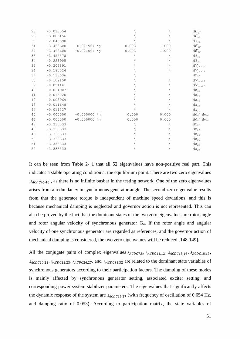
51

28 -3.018354 \ \ ΔEq3

29 -3.006456 \ \ ΔEd1

30 -2.845598 \ \ Δi12

31 -3.463600 +0.021567 *j 0.003 1.000 ΔEd2

32 -3.463600 -0.021567 *j 0.003 1.000 ΔEd2

33 -3.455578 \ \ Δi13

34 -0.228905 \ \ Δi23

35 -0.203891 \ \ ΔVpss31

36 -0.180524 \ \ ΔVpss33

37 -0.133536 \ Δx32

38 -0.102150 \ \ ΔVpss13

39 -0.051441 \ \ ΔVpss11

40 -0.034907 \ \ Δx42

41 -0.016020 \ \ Δx41

42 -0.003969 \ \ Δx43

43 -0.011648 \ \ Δx32

44 -0.011527 \ \ Δx31

45 -0.000000 +0.000000 *j 0.000 0.000 Δδ4\ Δω4

46 -0.000000 -0.000000 *j 0.000 0.000 Δδ4\ Δω4

47 -3.333333 \ \ Δx21

48 -3.333333 \ \ Δx12

49 -3.333333 \ \ Δx13

50 -3.333333 \ \ Δx23

51 -3.333333 \ \ Δx22

52 -3.333333 \ \ Δx23

It can be seen from Table 2- 1 that all 52 eigenvalues have non-positive real part. This

indicates a stable operating condition at the equilibrium point. There are two zero eigenvalues

𝜆𝐴𝐶𝐷𝐶45,46 , as there is no infinite busbar in the testing network. One of the zero eigenvalues

arises from a redundancy in synchronous generator angle. The second zero eigenvalue results

from that the generator torque is independent of machine speed deviations, and this is

because mechanical damping is neglected and governor action is not represented. This can

also be proved by the fact that the dominant states of the two zero eigenvalues are rotor angle

and rotor angular velocity of synchronous generator G4. If the rotor angle and angular

velocity of one synchronous generator are regarded as references, and the governor action of

mechanical damping is considered, the two zero eigenvalues will be reduced [148-149].

All the conjugate pairs of complex eigenvalues 𝜆𝐴𝐶𝐷𝐶7,8 , 𝜆𝐴𝐶𝐷𝐶 , , 𝜆𝐴𝐶𝐷𝐶 5, 6 , 𝜆𝐴𝐶𝐷𝐶 8, 9 ,

𝜆𝐴𝐶𝐷𝐶 0, , 𝜆𝐴𝐶𝐷𝐶 , , 𝜆𝐴𝐶𝐷𝐶 6, 7, and 𝜆𝐴𝐶𝐷𝐶 , are related to the dominant state variables of

synchronous generators according to their participation factors. The damping of these modes

is mainly affected by synchronous generator setting, associated exciter setting, and

corresponding power system stabilizer parameters. The eigenvalues that significantly affects

the dynamic response of the system are 𝜆𝐴𝐶𝐷𝐶 6, 7 (with frequency of oscillation of 0.654 Hz,

and damping ratio of 0.053). According to participation matrix, the state variables of

52

synchronous generator G1 have a dominant effect on the conjugate pair of 𝜆𝐴𝐶𝐷𝐶 6, 7 . In

consequence, these states should be considered primarily in attempt to improve network

damping characteristic.

The conjugate pairs of complex eigenvalues 𝜆𝐴𝐶𝐷𝐶 0, (with frequency of oscillation of 1.229

Hz, and damping ratio of 0.169), 𝜆𝐴𝐶𝐷𝐶 , (with frequency of oscillation of 1.265 Hz, and

damping ratio of 0.168), and 𝜆𝐴𝐶𝐷𝐶 6, 7 (with frequency of oscillation of 0.654 Hz, and

damping ratio of 0.053) are related to the rotor angle and rotor angular velocity of

synchronous generator G2, G3, and G1 respectively, if the rotor angle and rotor angular

velocity of synchronous generator G4 are regarded as reference. These oscillation

characteristic reflected by modal analysis can be further validated by simulation results in

section 2.6. The conjugate pairs of complex eigenvalues 𝜆𝐴𝐶𝐷𝐶 8, 9 are associated to the

transient electromagnetic force caused by field flux linkage in q-axis of synchronous

generator G1. The remaining conjugate pairs of complex eigenvalues 𝜆𝐴𝐶𝐷𝐶7,8 , and

𝜆𝐴𝐶𝐷𝐶 , are associated to the states of synchronous generator G4 and conjugate pairs

𝜆𝐴𝐶𝐷𝐶 5, 6 , and 𝜆𝐴𝐶𝐷𝐶 , are associated to the states of synchronous generator G2. The

incorporation of additional PSS can contribute to the damping of these modes since the

existing PSS are installed to synchronous generator G1, and G3 only.

2.6 Simulation Validation

The AC/DC test system as shown in Figure 2- 5 has been established in RSCAD to validate

the results of modal analysis. The power flow data, AC voltages, and impedance values are

based on 4-generator 2-area benchmark system model in [6] where same parameters are used

in 2.5.2.

The purpose of using RTDS-based simulation and testing platform is due to the fact that it

can provide an effective solution for such a development with the following benefits:

1. In the RSCAD environment (RSCAD is the specifically-designed software platform for

power system modelling and interfacing to RTDS hardware), the power electronic

devices can be represented using detailed models in close to practical devices. In this

way, it can reflect the steady-state and dynamic characteristics of power electronic

devices (including VSC FACTS and VSC HVDC devices);

53

2. With specifically-designed multiple processing units for digital simulation, the

computational capability of RTDS hardware can be powerful enough to achieve real-

time simulation. In doing so, the simulation efficiency of RTDS can satisfy the

requirements for multi-scenario detailed analysis of power electronic devices;

3. RTDS can provide the function of hardware-in-the-loop to realise the interactions

between the simulated virtual power networks in RSCAD and those physical protective

relays and hardware-based controllers.

2.6.1 Small Disturbances

Small disturbances (changes of reference) are applied to AC/DC test system to validate the

result of modal analysis to investigate small signal stability of the test system. A step

reference change is applied to VSC2, with V𝑑𝑐 𝑟𝑒𝑓 changes from 2.0 (p.u.) to 2.1 (p.u.) at 0.6s.

The dynamic response of rotor angular velocity difference of synchronous generators 1-4 in

response to the small disturbance are shown in Figure 2- 6. The damping frequency and

damping ratio of difference of synchronous generators seen from the figure are in line with

modal analysis results.

54

Figure 2- 6 Rotor angular velocity differences of synchronous generators 1-4.

The dynamic response of VSC related data of VSC1, VSC2, and VSC3, including DC voltage,

active power transfer, and AC voltage are shown in Figure 2- 7 to Figure 2- 9. It can be seen

from the figures that the DC voltages of all VSC reached a new steady state after a short

period of time while active power transfer and AC voltage recovers to their former value after

the disturbance. This is due to the control system of all VSC are set to AC voltage regulation

in q axis. The VSC2 is set to DC voltage regulation, while VSC1 and VSC3 are set to active

power transfer control.

55

Figure 2- 7 Dynamic response of VSC1 against small disturbance.

56



The dynamic response of DC network, including current of DC branch 12, 13 and 23 are

shown in Figure 2- 10. It can be seen from the figures that the currents of all DC braches

reach to a new steady states after a short period of time. And small oscillations of DC branch

13 are seen since no DC current flow controller is applied to DC network and active power

through branch 13 is not controlled. Stable dynamic performance against small disturbance

can be seen from the simulation results, which is in line with the modal analysis results.

57

Figure 2- 10 Dynamic response of DC network.

2.6.2 Large Disturbances

AC-System fault

A large disturbance is applied to test the stability of the system under large disturbances. A

10Ω single-line-to-ground (SLG) fault is simulated at PCC of VSC terminal 3 (primary side

of coupling transformer) at 0.15s lasting for 7 cycles (116 ms).


active power transfer, and AC voltage are shown in Figure 2- 11 to Figure 2- 13. It can be

58

seen from the figures that the DC voltages, active power transfer, and AC voltage of all VSC

recovers to their former values after the disturbance.

Figure 2- 11 Dynamic response of VSC1 against AC system fault.

59


60


The dynamic response of DC network, including currents of DC branch 12, 13 and 23 are


recover to its former values after the fault. The simulation results against large AC system

fault demonstrate that the system can endure large AC disturbance.

61

Figure 2- 14 Dynamic response of DC network against AC system fault.

DC Cable fault

For the testing of large disturbance at DC side, a 25Ω line-to-ground DC-cable fault is

simulated at DC-side of VSC3 at 0.15s lasting for 7 cycles (116 ms).


active power transfer, and AC voltage are shown in Figure 2- 15 to Figure 2- 17. It can be

seen from the figures that the DC voltages, active power transfer, and AC voltage of all VSC

recovers to their former values after the DC cable fault.

62

Figure 2- 15 Dynamic response of VSC1 against DC cable fault.

63


64


The dynamic response of DC network, including current of DC branch 12, 13 and 23 are


recover to its former values after the fault. The simulation results against DC cable fault

demonstrate that the system can endure large DC disturbance.

Figure 2- 18 Dynamic response of DC network against DC cable fault.

65

2.7 Summary

In this chapter, AC power system including synchronous generator with excitation system

and PSS, and network power flow has been modelled in dynamic and algebraic equations.

MTDC system without CFC, including VSC with its control system and generalized DC

network without CFC has been modelled in dynamic equations. Dynamic model of these two

subsystems have been linearized and formulated to form state-space representation of multi-

model system for small-signal stability analysis. An integrated AC/DC system that consists of

multiple synchronous generators with excitation system and PSS, multiple VSC converters,

and DC network without CFC, has been established. Small-signal model of test system has

been derived based on approaches in 2.2-2.4 and the eigenvalues of state-space representation

of test system have been calculated. Modal analysis of the eigenvalues results has been

performed to study small-signal stability of VSC-based MTDC system without CFC.

It can be found from eigenvalue results that all 52 eigenvalues have non-positive real part.

This indicates a stable operating condition at the considered operating point. There are two

zero eigenvalues, as there is no infinite bus bar in the testing network. One of the eigenvalue



because mechanical damping is neglected and governor action is not represented. If the rotor

angle and angular velocity of one synchronous machine are regarded as references, and the

governor action of mechanical damping is considered, the two zero eigenvalues will be

reduced. All the conjugate pairs of complex eigenvalues are related to the dominant state

variables of synchronous generators according to their participation factors. The damping of

these modes is mainly affected by synchronous generator setting, associated exciter setting,

and corresponding power system stabilizer parameters.

Simulations results of established AC/DC system against small disturbances in aspects of

damping frequency and damping ratio of difference of synchronous generators are in line

with modal analysis results. A stable operating condition around operating point is seen from

simulation results in RTDS/RSCAD against both small disturbance of change of reference

and large disturbances (including AC system faults, and DC cable faults), which is in line

with modal analysis results.

66

CHAPTER 3 SMALL-SIGNAL STABILITY ANALYSIS

OF VSC BASED MTDC SYSTEM WITH DC CFC

3.1 Introduction

This chapter presents the dynamic modelling of the integrated MTDC/AC system with

integration of CFC to study the small-signal stability of VSC-based MTDC system with CFC

and the potential interactions between CFC and VSC. In 3.2, the modelling of DC network

with CFC and its control system is presented in dynamic equations. The small-signal state-

space model of DC network with CFC is linearized around equilibrium point. Then the

linearized state-space model of the subsystem of DC network with CFC is merged into VSC-

based MTDC system without CFC presented in Chapter 2 to formulate multi-model system

with CFC. In 3.3, a test system that consists of multiple synchronous generators with

excitation system and PSS, multiple VSC converters, and DC network with CFC, is

established. Small-signal model of test system is derived based on approaches presented in

Chapter 2 and the eigenvalues of state-space representation of the test system are calculated.

Modal analysis of calculated eigenvalues in comparison between integrated AC/DC system

without/with CFC is implemented to study the impacts of the incorporation of CFC, and its

control parameters on small-signal stability of the integrated AC/DC system. Simulations

results of established AC/DC system against small disturbances and large disturbances

(including AC system faults, and DC cable faults) in RTDS/RSCAD are analysed to validate

modal analysis results. Eigenvalue trajectories are used to study the potential interactions

between CFC and VSC, including impacts of control parameters of CFC on VSC, and

impacts of control parameters of VSC on CFC.

3.2 Modelling, Linearization and Formulation of VSC Based MTDC

System with CFC

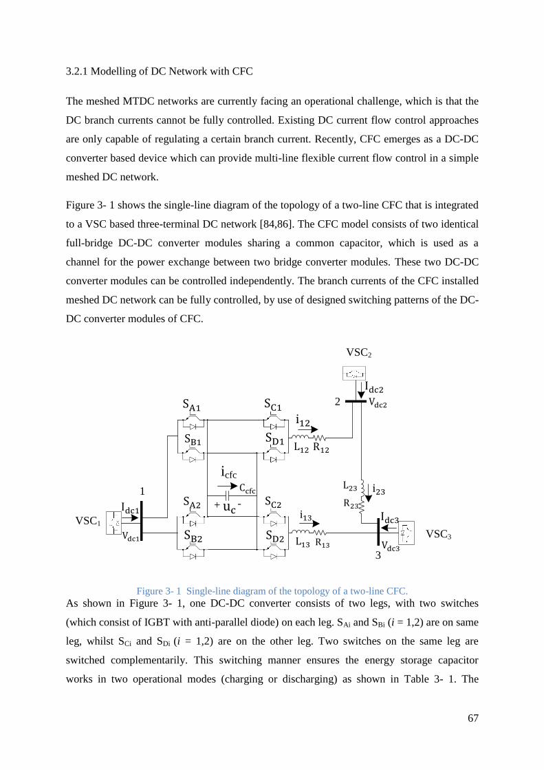
67

3.2.1 Modelling of DC Network with CFC

The meshed MTDC networks are currently facing an operational challenge, which is that the

DC branch currents cannot be fully controlled. Existing DC current flow control approaches

are only capable of regulating a certain branch current. Recently, CFC emerges as a DC-DC

converter based device which can provide multi-line flexible current flow control in a simple

meshed DC network.

Figure 3- 1 shows the single-line diagram of the topology of a two-line CFC that is integrated

to a VSC based three-terminal DC network [84,86]. The CFC model consists of two identical

full-bridge DC-DC converter modules sharing a common capacitor, which is used as a

channel for the power exchange between two bridge converter modules. These two DC-DC

converter modules can be controlled independently. The branch currents of the CFC installed

meshed DC network can be fully controlled, by use of designed switching patterns of the DC-

DC converter modules of CFC.

�

�

�

� �

�

�

�

+ -

VSC1

VSC2

VSC3

icfc

1

2

3

Figure 3- 1 Single-line diagram of the topology of a two-line CFC.

As shown in Figure 3- 1, one DC-DC converter consists of two legs, with two switches

(which consist of IGBT with anti-parallel diode) on each leg. SAi and SBi (i = 1,2) are on same

leg, whilst SCi and SDi (i = 1,2) are on the other leg. Two switches on the same leg are

switched complementarily. This switching manner ensures the energy storage capacitor

works in two operational modes (charging or discharging) as shown in Table 3- 1. The

68

capacitor is charging when both � and � are on, while the capacitor is discharging when

both � and � are on.

Table 3- 1 DC-DC converter operational modes

DC-DC CONVERTER OPERATIONAL MODES

Mode Capacitor State � � � �

1

Charging ON OFF OFF ON

2 Discharging OFF ON ON OFF

The target of the CFC control system is to maintain the voltage across the capacitor and to

control DC current of a certain DC transmission line branch, for example in this case.

The duty cycles of switch-on state of all the switches in two full-bridge module are shown in

Table 3- 2.

Table 3- 2 Switch duty cycles

SWITCH DUTY CYCLES

Switches � , � � , � � � � �

Duty Cycles da 1 − da d 1 − d d 1 − d

e12

VSC1

VSC2

VSC3

+ -

e13+ -

1

2

3

Figure 3- 2 Equivalent circuit of two-line CFC.

69

By this operation manner, the voltages across DC-DC converter in two DC branch, e and

e can be regarded as two voltage sources as shown in Figure 3- 2, and current through CFC

, can be summarized as in Table 3- 3.

Table 3- 3 Switching modes of CFC.

SWITCHING MODES OF CFC

Switching Mode Switches On Duty Cycle e

1 � , � a 0 0

2 � , � a

3 � , � a − −

4 � , � a4 0 0

Switching Mode Switches On Duty Cycle e

5 � , � b 0 0

6 � , � b

7 � , � b − −

8 � , � b4 0 0

The duty cycles in Table 3- 3 can be derived as follows:

𝑎 = 𝑚𝑖𝑛{𝑑𝑐 , 𝑑𝑎} (3. 1)

𝑎 = 𝑚𝑎𝑥{𝑑𝑎 − 𝑑𝑐 , 0} (3. 2)

𝑎 = 𝑚𝑖𝑛{𝑑𝑐 − 𝑑𝑎 , 0} (3. 3)

𝑎4 = 1 − 𝑚𝑎𝑥{𝑑𝑎, 𝑑𝑐 } (3. 4)

𝑏 = 𝑚𝑖𝑛{𝑑𝑐 , 𝑑𝑎} (3. 5)

𝑏 = 𝑚𝑎𝑥{𝑑𝑎 − 𝑑𝑐 , 0} (3. 6)

𝑏 = 𝑚𝑖𝑛{𝑑𝑐 − 𝑑𝑎 , 0} (3. 7)

𝑏4 = 1 − 𝑚𝑎𝑥{𝑑𝑎, 𝑑𝑐 } (3. 8)

Hence the voltages across DC-DC converter in two coupling DC branch e , and e can be

expressed with corresponding duty cycles as:

70

𝑒 = (𝑎 − 𝑎 )𝑢𝑐 = (𝑑𝑎 − 𝑑𝑐 )𝑢𝑐 (3. 9)

𝑒 = (𝑏 − 𝑏 )𝑢𝑐 = (𝑑𝑎 − 𝑑𝑐 )𝑢𝑐 (3. 10)

And by considering the charging and discharging states of the capacitor within a switching

cycle, the dynamic of capacitor can be obtained as:

𝐶𝑑𝑢𝑐

𝑑𝑡= (𝑎 − 𝑎 )𝑖 + (𝑏 − 𝑏 )𝑖 = (𝑑𝑎 − 𝑑𝑐 )𝑖 + (𝑑𝑎 − 𝑑𝑐 )𝑖 (3. 11)

The target of control system of the two-line CFC is to regulate the duty cycle ratio of the

switches so that the voltage across the capacitor is maintained and the current of DC branch

(𝑖 in this study) is controlled.

Figure 3- 3 shows the architecture of CFC control system to output duty cycle ratio of the

switches. The DC branch current 𝑖 , reference of DC branch current 𝑖 ∗ , capacitor

voltage 𝑢𝑐 , and reference of capacitor voltage 𝑢𝑐∗ are inputs of the control system. The

difference of 𝑖 ∗ and 𝑖 is inputted into a PI control loop and the first limitation block. Then

the output of the first limitation block (which yields 𝑑𝑎 − 𝑑𝑐 ), is subtracted from 𝑑𝑎 and

inputted into the second limitation block. The output signal of the second limitation block is

𝑑𝑐 . Similarly, the difference of 𝑢𝑐∗ and 𝑢𝑐 is inputted into a PI control loop and the first

limitation block. Then the output of the first limitation block (which yields 𝑑𝑎 − 𝑑𝑐 ), is

subtracted from 𝑑𝑎 and inputted into the second limitation block. The output signal of the

second limitation block is 𝑑𝑐 . And by use of same kind of gate signal generator that is

commonly used in VSC, the gate signals GS , and GS to control the switches are generated.

Σ+

-

PI Σ+

-Gate Signal

Generator-1

Σ+

-

PI Σ

+

-

Gate Signal

Generator

dc1

dc2

Figure 3- 3 Architecture of CFC control system.

In this way, the duty cycle reference 𝑑𝑐 , and 𝑑𝑐 can be obtained as:

𝑑𝑐 = 𝑑𝑎 − 𝑘𝑝𝑐 (−𝑖 ∗ + 𝑖 ) − 𝑘𝑖𝑐 ∫(−𝑖

∗ + 𝑖 )𝑑𝑡

71

= 𝑑𝑎 − 𝑘𝑝𝑐 (−𝑖 ∗ + 𝑖 ) − 𝑘𝑖𝑐 𝑦 (3. 12)

𝑑𝑐 = 𝑑𝑎 − 𝑘𝑝𝑐 (𝑢𝑐∗ − 𝑢𝑐) − 𝑘𝑖𝑐 ∫(𝑢𝑐

∗ − 𝑢𝑐)𝑑𝑡

= 𝑑𝑎 − 𝑘𝑝𝑐 (𝑢𝑐∗ − 𝑢𝑐) − 𝑘𝑖𝑐 𝑦 (3. 13)

where

𝑘𝑝𝑐 , 𝑘𝑖𝑐 , 𝑘𝑝𝑐 , and 𝑘𝑖𝑐 : the proportional and integral gains of the PI control loops of CFC

control system

𝑦 and 𝑦 : auxiliary state variables to represent integral parts of the PI control loops

Applying Kirchhoff's voltage law, the dynamic equations of all DC braches of the three-

terminal DC network with CFC can be derived as:

𝐿

𝑑𝑖

𝑑𝑡+ 𝑅 𝑖 = 𝑉𝑑𝑐 − 𝑉𝑑𝑐 − 𝑒 (3. 14)

𝐿

𝑑𝑖

𝑑𝑡+ 𝑅 𝑖 = 𝑉𝑑𝑐 − 𝑉𝑑𝑐 − 𝑒 (3. 15)

𝐿

𝑑𝑖

𝑑𝑡+ 𝑅 𝑖 = 𝑉𝑑𝑐 − 𝑉𝑑𝑐 (3. 16)

The final mathematical dynamic equations of DC network with CFC can be obtained by

substitute (3.9)-(3.10), (3.12), and (3.13), into (3.11), and (3.14)-(3.16), with auxiliary state

variable dynamics as follows:

𝑑𝑦

𝑑𝑡= −𝑖

∗ + 𝑖 (3. 17)

𝑑𝑦

𝑑𝑡= 𝑢𝑐

∗ − 𝑢𝑐 (3. 18)

3.2.2 Linearization of DC Network with CFC

The linearization of the dynamic equations of DC network with CFC (3.11), (3.14)-(3.18) can

be expressed as follows:

72

∆�̇�𝐶𝐹𝐶 = 𝑨𝑪𝑭𝑪∆𝑥𝐶𝐹𝐶 + 𝑨𝑪𝑭𝑪𝟐∆𝑥𝑉𝑑𝑐 + 𝑬𝑪𝑭𝑪∆𝑢𝐶𝐹𝐶 (3. 19)

where

∆𝑥𝐶𝐹𝐶 = [∆𝑖 , ∆𝑖 , ∆𝑖 , ∆𝑢𝑐 , ∆𝑦 , ∆𝑦 , ]𝑇 (3. 20)

∆𝑥𝑉𝑑𝑐 = [∆𝑉𝑑𝑐 , ∆𝑉𝑑𝑐 , ∆𝑉𝑑𝑐 ]𝑇 (3. 21)

∆𝑢𝐶𝐹𝐶 = [∆𝑖 ∗ , ∆𝑢𝑐

∗]𝑇 (3. 22)

3.2.3 Formulation of Multi-Model System

The independent linearized models of AC power system, MTDC system without CFC, and

DC network with CFC studied in 2.4.1, 2.4.2, and 3.2.2 respectively, are formulated into a

whole multi-model system, in order to investigate the small-signal stability of VSC–based

MTDC system with CFC.

The DC network with CFC is integrated into MTDC system without CFC via VSC converters

connected at VSC terminal of DC network, when CFC is installed into DC network. The

state-space representation of DC network with CFC obtained in 3.2.2 is merged with the

state-space representation of VSC obtained in 2.4.2 as follows:

∆�̇�𝑀𝑇𝐷𝐶𝐶𝐹𝐶 = 𝑨𝑴𝑻𝑫𝑪𝑪𝑭𝑪∆𝑥𝑀𝑇𝐷𝐶𝐶𝐹𝐶 + 𝑩𝑴𝑻𝑫𝑪𝑪𝑭𝑪∆𝑉𝑙 + 𝑬𝑴𝑻𝑫𝑪𝑪𝑭𝑪∆𝑢𝑀𝑇𝐷𝐶𝐶𝐹𝐶 (3. 23)

where

∆𝑥𝑀𝑇𝐷𝐶𝐶𝐹𝐶 = [∆𝑥𝑉𝑆𝐶𝑇 , ∆𝑥𝐶𝐹𝐶

𝑇]𝑇 (3. 24)

∆𝑢𝑀𝑇𝐷𝐶𝐶𝐹𝐶 = [∆𝑥𝑉𝑆𝐶𝑇 , ∆𝑢𝐶𝐹𝐶

𝑇]𝑇 (3. 25)

Finally, the linearized dynamic equations of MTDC system with CFC (3.23) can be merged

with the linearized dynamic equations of all synchronous generators (2.52) using the same

approach that presented in 2.4.3 as follows:

∆�̇�𝐴𝐶𝐷𝐶𝐶𝐹𝐶 = 𝑨𝑨𝑪𝑫𝑪𝑪𝑭𝑪∆𝑋𝐴𝐶𝐷𝐶𝐶𝐹𝐶 + 𝑩𝑨𝑪𝑫𝑪𝑪𝑭𝑪∆𝑈𝐴𝐶𝐷𝐶𝐶𝐹𝐶 (3. 26)

where

∆𝑋𝐴𝐶𝐷𝐶𝐶𝐹𝐶 = [∆𝑥𝑆𝐺𝐴𝑇 , ∆𝑥𝑀𝑇𝐷𝐶𝐶𝐹𝐶

𝑇]𝑇 (3. 27)

73

∆𝑈𝐴𝐶𝐷𝐶𝐶𝐹𝐶 = [∆𝑢𝑔𝑇 , ∆𝑢𝑀𝑇𝐷𝐶𝐶𝐹𝐶

𝑇]𝑇 (3. 28)

3.3 Impacts of CFC on Small-Signal Stability of the Integrated AC/DC

System

As CFC is integrated into MTDC system, the small-signal stability of the integrated AC/DC

system is studied in this section to investigate the potential impacts of CFC that might be

brought in. The modified test system is described in 3.3.1 with CFC installed into DC

network. The modal analysis for the modified integrated AC/DC system is studied to

investigate the small-signal stability in 3.3.2. The dynamic simulations in case of small

disturbances and large disturbances are performed in 3.3.3 to validate modal analysis results.

Finally, the impacts of the incorporation of CFC on existing MTDC system is studied in 3.3.4.

3.3.1 Test System

The single-line diagram of the topology of CFC integrated AC/DC system is shown in Figure

3- 4. The modified system is based on the MTDC system established in 2.5.1 which is added

with a two-line CFC. As shown in Figure 3- 4, the CFC is located at the DC side of VSC1 to

control the current flow of DC branch i12 and i13. The parameters of CFC are listed in

Appendix A.9 while other parameters of existing MTDC system are the same with the test

system in Chapter 2.

74

G4

Load

G3

Load

110 km 110 km 10 km 25 km

G1 G2

25 km 10 km

Idc3

Vdc3

i13

L13 R13

i23L23

R23

VSC1

VSC2

VSC3�

�

�

� �

�

�

� + -

icfc

1 2 34

5

6 7 8 9 10

11

Figure 3- 4 Single-line diagram of the topology of CFC integrated AC/DC system.

3.3.2 Modal Analysis

In order to illustrate the impacts of the incorporation of CFC on small-signal stability of the

integrated AC/DC system, eigenvalue analysis is implemented for the system with CFC.

The complete state-space matrix 𝑨𝑨𝑪𝑫𝑪𝑪𝑭𝑪 has a dimension of 55 × 55, which consists of

sub state-space matrix of two synchronous generators with excitation system (2 × (7 × 7) =

2 × (6 + 1) × (6 + 1) ), sub state-space matrix of two synchronous generators with

excitation system and PSS (2 × (10 × 10) = 2 × (6 + 1 + 3) × (6 + 1 + 3) ), sub state-

space matrix of three VSC converters (3 × (5 × 5)), sub state-space matrix of DC network

(3 × 3)(the state variables are ∆𝑖 , ∆𝑖 , ∆𝑖 ), and sub state-space matrix of CFC (3 × 3)(the

state variables are ∆𝑢𝑐, ∆𝑦 , ∆𝑦 ). There are 52 eigenvalues for the system without CFC as

presented in 2.5.2, and 55 eigenvalues of the system with CFC. The additional three states

result from the CFC capacitor and 2 integral controllers of CFC (∆𝑢𝑐, ∆𝑦 , ∆𝑦 ).

By use of the approach to compute eigenvalues presented in 2.5.2, the calculated eigenvalues

𝝀𝑨𝑪𝑫𝑪𝑪𝑭𝑪 of 𝑨𝑨𝑪𝑫𝑪𝑪𝑭𝑪 are shown in Table 3- 4. The frequency of oscillation, damping ratio

and dominant state of all conjugate pairs of complex eigenvalues are also provided in Table

3- 4.

Table 3- 4 Eigenvalue results of CFC integrated AC/DC system

75

No. *Eigenvalue *Frequency *Damping Ratio *Dominant State

1 -989.996909 \ \ ΔEfd4

2 -992.295149 \ \ ΔEfd1

3 -995.595105 \ \ ΔEfd1

4 -995.707401 \ \ ΔEfd4

5 -29.207818 +79.733757 *j 12.690 0.344 Δi13

6 -29.207818 -79.733757 *j 12.690 0.344 Δi13

7 -36.172771 +74.960903 *j 11.930 0.435 Δi12

8 -36.172771 -74.960903 *j 11.930 0.435 Δi12

9 -50.413402 \ \ ΔVpss23

10 -50.366193 \ \ ΔVpss21

11 -21.427289 +15.161162 *j 2.413 0.816 Δφ1d4

12 -21.427289 -15.161162 *j 2.413 0.816 Δφ1d4

13 -40.284553 \ \ ΔVdc3

14 -36.147588 +0.024697 *j 0.004 1.000 Δφ2q4

15 -36.147588 -0.024697 *j 0.004 1.000 Δφ2q4

16 -32.194893 \ \ Δφ1d2

17 -31.405286 \ \ Δφ1d4

18 -30.737465 +0.158230 *j 0.025 1.000 Δφ2q2

19 -30.737465 -0.158230 *j 0.025 1.000 Δφ2q2

20 -20.867725 +9.466367 *j 1.507 0.911 ΔEq1

21 -20.867725 -9.466367 *j 1.507 0.911 ΔEq1

22 -1.324673 +7.721606 *j 1.229 0.169 Δδ2\ Δω2

23 -1.324673 -7.721606 *j 1.229 0.169 Δδ2\ Δω2

24 -1.353150 +7.949151 *j 1.265 0.168 Δδ3\ Δω3

25 -1.353150 -7.949151 *j 1.265 0.168 Δδ3\ Δω3

26 -13.782411 \ \ Δi23

27 -10.373649 \ \ ΔEq1

28 -10.232547 \ \ ΔEq4

29 -0.218588 +4.107533 *j 0.654 0.053 Δδ1\ Δω1

30 -0.218588 -4.107533 *j 0.654 0.053 Δδ1\ Δω1

31 -0.554283 +0.930014 *j 0.148 0.512 Δy2

32 -0.554283 -0.930014 *j 0.148 0.512 Δy2

33 -3.018345 \ \ ΔEd3

34 -3.006447 \ \ ΔEd1

35 -3.462913 +0.020338 *j 0.003 1.000 ΔEd2

36 -3.462913 -0.020338 *j 0.003 1.000 ΔEd2

37 -0.204027 \ \ ΔVpss31

38 -0.180561 \ \ ΔVpss33

39 -0.092289 +0.087653 *j 0.014 0.725 Δx32

40 -0.092289 -0.087653 *j 0.014 0.725 Δx32

41 -0.133912 \ \ Δx31

42 -0.102123 \ \ ΔVpss13

43 -0.051550 \ \ ΔVpss11

44 -0.034554 \ \ Δx42

45 -0.016087 \ \ Δx41

46 -0.011626 \ \ Δx31

47 -0.003970 \ \ Δx43

48 0.000000 +0.000000 *j 0.000 -0.000 Δδ4\ Δω4

49 0.000000 -0.000000 *j 0.000 -0.000 Δδ4\ Δω4

50 -3.333333 \ \ Δx21

51 -3.333333 \ \ Δx13

52 -3.333333 \ \ Δx22

53 -3.333333 \ \ Δx12

54 -3.333333 \ \ Δx11

55 -3.333333 \ \ Δx23

CFC

related

VSC

related

Generator

related

76

It can be seen from Table 3- 4 that all 55 eigenvalues have non-positive real part. This

indicates a stable operating condition around the equilibrium point. There are two zero

eigenvalues 𝜆𝐴𝐶𝐷𝐶48,49 , as there is no infinite busbar in the testing network. These two zero

eigenvalues are caused by same reasons of AC/DC system without CFC presented in Chapter

2. One of the zero eigenvalues arises from a redundancy in synchronous generator angle. The

second zero eigenvalue results from that the generator torque is independent of machine

speed deviations, and this is because mechanical damping is neglected and governor action is

not represented. This can also be proved by the fact that the dominant states of the two zero

eigenvalues are rotor angle and rotor angular velocity of synchronous generator G4. If the

rotor angle and angular velocity of one synchronous generator are regarded as reference, and

the governor action of mechanical damping is considered, the two zero eigenvalues will be

reduced [148-149].

The conjugate pairs of complex eigenvalues 𝜆𝐴𝐶𝐷𝐶 , , 𝜆𝐴𝐶𝐷𝐶 4, 5, 𝜆𝐴𝐶𝐷𝐶 8, 9 to 𝜆𝐴𝐶𝐷𝐶 4, 5 ,

𝜆𝐴𝐶𝐷𝐶 9, 0 , and 𝜆𝐴𝐶𝐷𝐶 5, 6 are related to the dominant state variables of synchronous

generators according to their participation factors. The damping of these modes is mainly

affected by synchronous generator settings, associated exciter settings, and corresponding

PSS parameters. The eigenvalues that significantly affects the dynamic response of the

system are 𝜆𝐴𝐶𝐷𝐶 9, 0 (with frequency of oscillation of 0.654 Hz, and damping ratio of 0.053).

According to participation matrix, the state variables of synchronous generator G1 have a

dominant effect on the conjugate pair of 𝜆𝐴𝐶𝐷𝐶 9, 0. In consequence, these states should be

considered primarily in attempt to improve network damping characteristic. Compared to

eigenvalue results of AC/DC system without CFC presented in Table 2- 1, there is no

significant changes of values of these synchronous generator related conjugate pairs due to

the incorporation of CFC. This presents that the corporation of CFC has no significant

impacts on dynamic stability of multi synchronous generators.

The conjugate pairs of complex eigenvalues 𝜆𝐴𝐶𝐷𝐶5,6, 𝜆𝐴𝐶𝐷𝐶7,8 , and 𝜆𝐴𝐶𝐷𝐶 , are related to

the dominant state variables of DC networks with CFC according to their participation

factors. The dominant state of 𝜆𝐴𝐶𝐷𝐶7,8 is i12 which is controlled by CFC. The dominant state

of 𝜆𝐴𝐶𝐷𝐶 , is CFC y2 which represents the state variable of CFC integral controller. Based

on these results, the incorporation of CFC results in the emergence of CFC related

eigenvalues which means the oscillations of relevant DC network states are expected.

77

It should be noted that the dominant state of 𝜆𝐴𝐶𝐷𝐶 9,40 is VSC2 Δx32 which represents the

state variable of the integral controller of VSC2. This interesting phenomenon indicates that

the incorporation of CFC can even cause the emergence of VSC related conjugate pairs. And

the emergence of new oscillations of relevant VSC states is expected. The dynamic stability

of VSC is affected by the integration of CFC into DC network.

(a) Clustering of eigenvalues (b) Highlighted eigenvalues

Figure 3- 5 Eigenvalues of the integrated AC/DC system without CFC.

(a) Clustering of eigenvalues (b) Highlighted eigenvalues

Figure 3- 6 Eigenvalues of the integrated AC/DC system with CFC.

Figure 3- 5 shows a plot of eigenvalues of system without CFC while Figure 3- 6 shows a

plot of eigenvalues of system with CFC. The dominant states and the associated pairs of

eigenvalues are highlighted in Figure 3- 5 (b) for the system without CFC and in Figure 3- 6

(b) for the system with CFC. Compared to system without CFC as shown in Figure 3- 5 (b), it

can be seen that the system with CFC (as shown in Figure 3- 6 (b)) has 3 additional conjugate

pairs of eigenvalues, which are dominated by state variables of DC branch currents , ,

and CFC integral controller auxiliary state y . Also, the integration of CFC has small

impacts on the synchronous generator related eigenvalues as there are no significant changes

in the placements of these eigenvalues. However, the integration of CFC leads to the

generator

𝑖 𝑖 CFC 𝑦

generator VSC2 𝑥

78

changing of VSC controller related eigenvalues from the pure negative real values to the

conjugate pair of eigenvalues with negative real part, as highlighted by VSC2 x in Figure 3-

6 (b). This change indicates VSC controller related system oscillations for the system with

CFC. The reason of this change can be the potential interactions between CFC and adjacent

VSC.

From Figure 3- 6, the critical modes which have major impacts on small signal performance

of the system are associated with CFC auxiliary statey , VSC2 auxiliary state x , and the

angle and rotating speed of Synchronous Generator 1.

3.3.3 Impacts of Control Parameters of CFC

It has been found from modal analysis presented in 3.3.2 that the integration of CFC can

affect dynamic stability of the integrated AC/DC system, especially on those VSC state

variable related modes. In this section the potential effects of the control parameters of CFC

(different values of the gains of CFC controller including k𝑝𝑐 , k𝑖𝑐 , k𝑝𝑐 , and k𝑖𝑐 ) on small-

signal stability of integrated AC/DC systems are studied.

The stable/unstable setting ranges of k𝑝𝑐 , k𝑖𝑐 , k𝑝𝑐 , and k𝑖𝑐 are obtained by procedures

shown in Figure 3- 7. As shown in Table 3- 5 to Table 3- 7, the stable/unstable setting ranges

of k𝑖𝑐 , k𝑝𝑐 , and k𝑖𝑐 derived following these procedures are listed. For the given test system

described in 3.3.1, the system is stable for 0.001 ≤ k𝑝𝑐 ≤ 1000 by use of the procedures

shown in Figure 3- 7.

79

Step 1 Select one of the control gain

from kpc1,kic1,kpc2,kic2,

Step 2 Input stable operating point from

simulation results

Step 3 Set the domain of definition of

selected control gain and its step size

Step 6 Scan the values of selected control

gain from the domain of definition

Step 4 Judge

If all values of selected gain

in domain of definition

are scanned

Step 5 Output

the stable and unstable operating range

of selected control gain

Step 8 Judge

If all real part of all eigenvalues

are negative

Step 7 Compute eigenvalues of system

under current value of control gain

Step 9 Update stable

operating range with

current value

Step 10 Update unstable

operating range with

current value

All values scanned

Not all

scanned

All negative

Positive real part

Figure 3- 7 Flowchart to obtain stable/unstable operating range of control gains.

Table 3- 5 Setting ranges of Kic1 on the integrated MTDC/AC system dynamics

SETTING RANGES OF K𝑖𝑐 ON THE INTEGRATED MTDC/AC SYSTEM DYNAMICS

Value Stability

ki ≤ 2.25 Stable

ki ≥ 2.25 unstable, 2 positive eigenvalues are seen

Table 3- 6 Setting ranges of Kpc2 on the integrated MTDC/AC system dynamics

SETTING RANGES OF K𝑝𝑐 ON THE INTEGRATED MTDC/AC SYSTEM DYNAMICS

Value Stability

kp ≤ 0.231 unstable, 1 positive pair of eigenvalues

kp ≥ 0.231 Stable

Table 3- 7 Setting ranges of Kic2 on the integrated MTDC/AC system dynamics

SETTING RANGES OF K𝑖𝑐 ON THE INTEGRATED MTDC/AC SYSTEM DYNAMICS

Value Stability

ki ≤ 0.73 unstable, 1 positive pair of eigenvalues

80

ki ≥ 0.73 stable

For the sake of illustration, proportional gain k𝑝𝑐 is selected as an example to investigate

system dynamic stability when CFC controller gains are changed. Table 3- 8 lists three

different values of k𝑝𝑐 (k𝑝𝑐 = 0.01,0.1, and 1) and relevant modes. The corresponding

values of λ31,32 are 0.16 ± j1.07, 0.09 ± j1.08, and -0.55±j0.93. The system is stable only

when k𝑝𝑐 ≥ 1 (𝜆 , = −0.55 ± j0.93).

Table 3- 8 Impacts of Kpc2 on the integrated MTDC/AC system dynamics

IMPACT OF K𝑝𝑐 ON THE INTEGRATED MTDC/AC SYSTEM DYNAMICS

Value λ , Stability

kp = 0.01 0.16 ± j1.07 unstable, 1 positive pair of eigenvalues

kp = 0.1 0.09 ± j1.08 unstable, 1 positive pair of eigenvalues

kp = 1 −0.55 ± j0.93 stable

The time-domain simulations in Figure 3- 8 are in line with the results shown in Table 3- 8

when a small change of the reference is applied ( 𝑟𝑒𝑓 changes from 0.55 kA to 0.50 kA at

0.5 s). Stable system dynamics can be achieved only when k𝑝𝑐 = 1. Unstable oscillations are

observed for k𝑝𝑐 = 0.1and k𝑝𝑐 = 0.01. It can also be seen that large k𝑝𝑐 decreases the

oscillation frequency and the settling time. The value of k𝑝𝑐 has significant effects on state

variables , and y . These results demonstrate that the control parameters of CFC may cause

instability of the system if they are not carefully-tuned.

(a) Current of DC branch 12.

81

(b) Auxiliary variable y2.

Figure 3- 8 Dynamics of DC network under different DC CFC control parameters.

3.3.4 Dynamic Simulation Validation

The AC/DC test system as shown in Figure 3- 4 has been established in RSCAD to validate

the results of modal analysis. The power flow data, AC voltages, and impedance values are

based on 4-generator 2-area benchmark system model in [6] while parameters of the DC

network and CFC are shown in Appendix A.9.

Small disturbances

Figure 3- 9 shows the dynamic behaviour of the system in response to a step reference change

applied to CFC ( 𝑟𝑒𝑓 changes from 0.55 kA to 0.50 kA at 0.15 s). It can be seen from Figure

3- 9 that the controlled current of DC branch 12 decreases by 0.05 kA and the current of DC

branch 13 increases by 0.05 kA. The total DC current through VSC1 remains unchanged. The

voltage of DC capacitor returns to its reference value after the small disturbance. There are no

significant changes in VSC related variables (DC voltage of VSC2, active power of VSC1 and

VSC3). Stable dynamic performance can be seen from the simulation results, which is in line

with the modal analysis results.

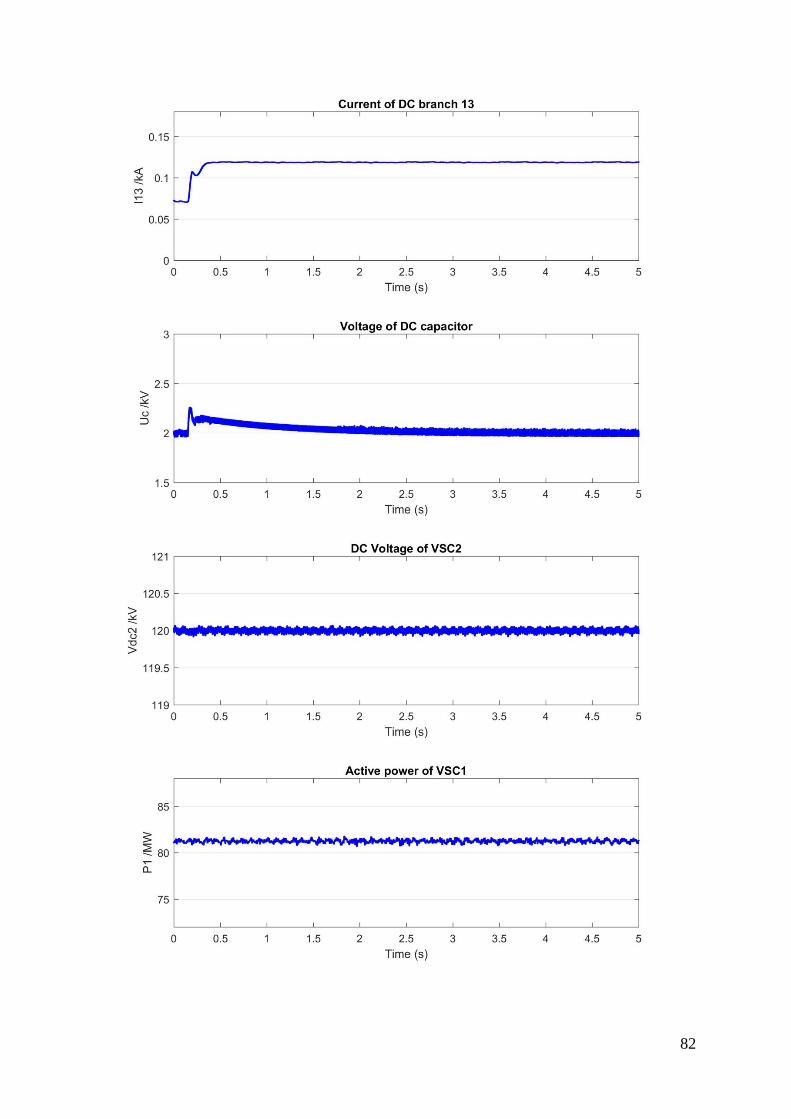
82

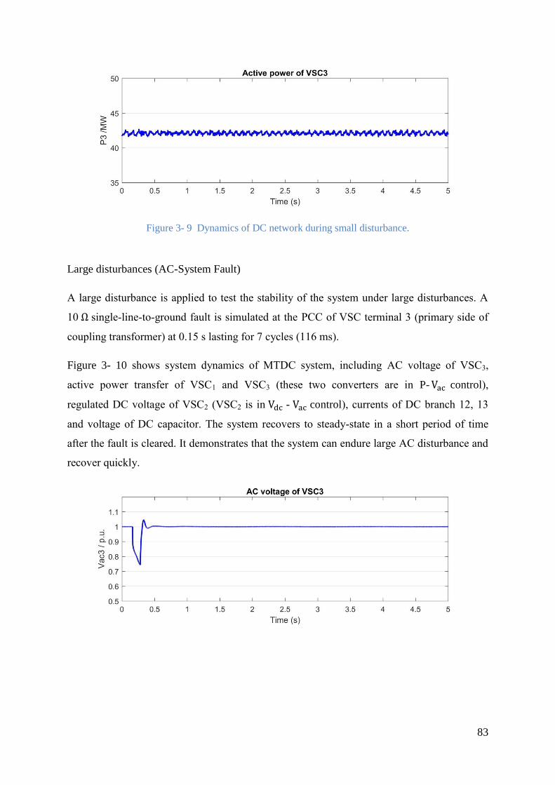
83

Figure 3- 9 Dynamics of DC network during small disturbance.

Large disturbances (AC-System Fault)

A large disturbance is applied to test the stability of the system under large disturbances. A

10 Ω single-line-to-ground fault is simulated at the PCC of VSC terminal 3 (primary side of

coupling transformer) at 0.15 s lasting for 7 cycles (116 ms).

Figure 3- 10 shows system dynamics of MTDC system, including AC voltage of VSC3,

active power transfer of VSC1 and VSC3 (these two converters are in P-Va control),

regulated DC voltage of VSC2 (VSC2 is in V - Va control), currents of DC branch 12, 13

and voltage of DC capacitor. The system recovers to steady-state in a short period of time

after the fault is cleared. It demonstrates that the system can endure large AC disturbance and

recover quickly.

84

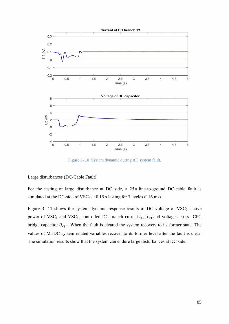
85

Figure 3- 10 System dynamic during AC system fault.

Large disturbances (DC-Cable Fault)

For the testing of large disturbance at DC side, a 25Ω line-to-ground DC-cable fault is

simulated at the DC-side of VSC3 at 0.15 s lasting for 7 cycles (116 ms).

Figure 3- 11 shows the system dynamic response results of DC voltage of VSC2, active

power of VSC1 and VSC3, controlled DC branch current 𝑖 , 𝑖 and voltage across CFC

bridge capacitor 𝑈𝑐𝑓𝑐. When the fault is cleared the system recovers to its former state. The

values of MTDC system related variables recover to its former level after the fault is clear.

The simulation results show that the system can endure large disturbances at DC side.

86

87

Figure 3- 11 System dynamic during DC cable fault.

3.4 Interactions between CFC and VSC

Based on the interesting phenomenon discovered from modal analysis presented in 3.3.2,

further research in potential interactions between CFC and VSC in aspects of system dynamic

stability is implemented in this section. In 3.4.1, the investigation of impacts of control

parameters of CFC control system on VSC is studied. In 3.4.2, the investigation of impacts of

control parameters of VSC control system on CFC is studied

3.4.1 Impacts of Control Parameters of CFC on VSC

As shown in Figure 3- 12, eigenvalue trajectory study is used to plot the movements of

critical conjugate pairs so that the impacts of changing control parameters of CFC on VSC

related modes are presented. In Figure 3- 12, the control gain k𝑝𝑐 varies from 0 (p.u.) to 1000

(p.u.) while the values of other control gains of CFC remain the same. The purple arrows

indicate the movement of conjugate pairs resulting from this variation of k𝑝𝑐 . As shown in

Figure 3- 12 (a). The imaginary parts of CFC related conjugate pairs ( 𝑖 and 𝑖 ) decrease

88

as k𝑝𝑐 increases, which indicate greater damping ratios of CFC related states. As shown in

Figure 3- 12 (a), two new VSC related conjugate pairs 𝑉𝑑𝑐 and 𝑉𝑑𝑐 (highlighted in blue)

emerge as k𝑝𝑐 increases. The movements of VSC related pairs ( 𝑉𝑑𝑐 , 𝑉𝑑𝑐 , and VSC 𝑥 ) as

shown in Figure 3- 12 (a)-(b) clearly present the impacts of CFC on VSC. The two conjugate

pairs of 𝑉𝑑𝑐 and 𝑉𝑑𝑐 move towards left half of s-plane which indicates greater damping

ratios of VSC related states 𝑉𝑑𝑐 and 𝑉𝑑𝑐 . The conjugate pairs of VSC 𝑥 move towards

right hand side indicating less damping ratios of VSC 𝑥 . As shown in Figure 3- 12 (a)-(b),

there are no significant movements of generator related poles, which indicates CFC has no

significant impacts on synchronous generator related states.

(a)

(b)

VSC x

𝑖

𝑖

𝑖

𝑖

𝑉𝑑𝑐

𝑉𝑑𝑐

generator

89

Figure 3- 12 Eigenvalue trajectories of various CFC control parameter kpc2.

Based on eigenvalue trajectory studies of CFC control gains, it can be summarised that the

variation of CFC controller can affect dynamic stability of CFC and VSC related modes.

These impacts of CFC on VSC can result in different damping characteristic of VSC related

states, as CFC controller changes.

As listed in Table 3- 9, three cases of different CFC control parameters are designed based on

eigenvalue trajectory studies of various CFC control gains, to investigate their effects on the

VSC controller related modes.

Case 1: the control system of CFC is disabled as the base case to represent system without

CFC control system.

Case 2: the gains of CFC control system are set the same as those in [84] ( 𝑘𝑝𝑐 = 1, 𝑘𝑖𝑐 =

1 , 𝑘𝑝𝑐 = 1 , 𝑘𝑖𝑐 = 1), to represent normal settings. The oscillations of VSC2 controller

related modes are seen from Table 3- 9. The AC/DC system is stable for the first two cases.

Case 3: the gains of CFC control system are changed ( 𝑘𝑝𝑐 = 0.01, 𝑘𝑖𝑐 = 1000, 𝑘𝑝𝑐 =

1, 𝑘𝑖𝑐 = 1000), to represent extreme or possible fault condition of CFC control system. One

conjugate pair of eigenvalues with positive real part is seen, which indicates small-signal

instability.

Table 3- 9 Impacts of control parameters of CFC on VSC2 related modes.

IMPACT OF CONTROL PARAMETERS OF DC CFC ON VSC2 RELATED MODES

Related Eigenvalues Stability

Case 1 −0.13,−0.017(λ 9,4 ) Stable

Case 2 −0.09 ± j0.09(λ 9,40) Stable

Case 3 0.02 ± j0.10(λ 8, 9) unstable, 1 positive pair of eigenvalues

Figure 3- 13 shows time-domain simulation results for the three cases. As shown in Figure 3-

13, a small perturbation (DC branch current control reference 𝑖 ∗ changes from 0.55 kA to

0.5 kA) is applied to CFC at 0.15s. For Case 1, no significant change of VSC2 auxiliary state

variable 𝑥 is observed because the CFC control system is disabled. For Case 2, a small

increase of 𝑥 at 0.2s can be seen. Then the value of 𝑥 recovers to the pre-disturbance level

after a period time of oscillations. For Case 3, large unstable oscillations are seen.

Simulation results are in line with modal analysis results in Table 3- 9, and illustrate that the

CFC control system can affect dynamic performance of VSC converter controller. This effect

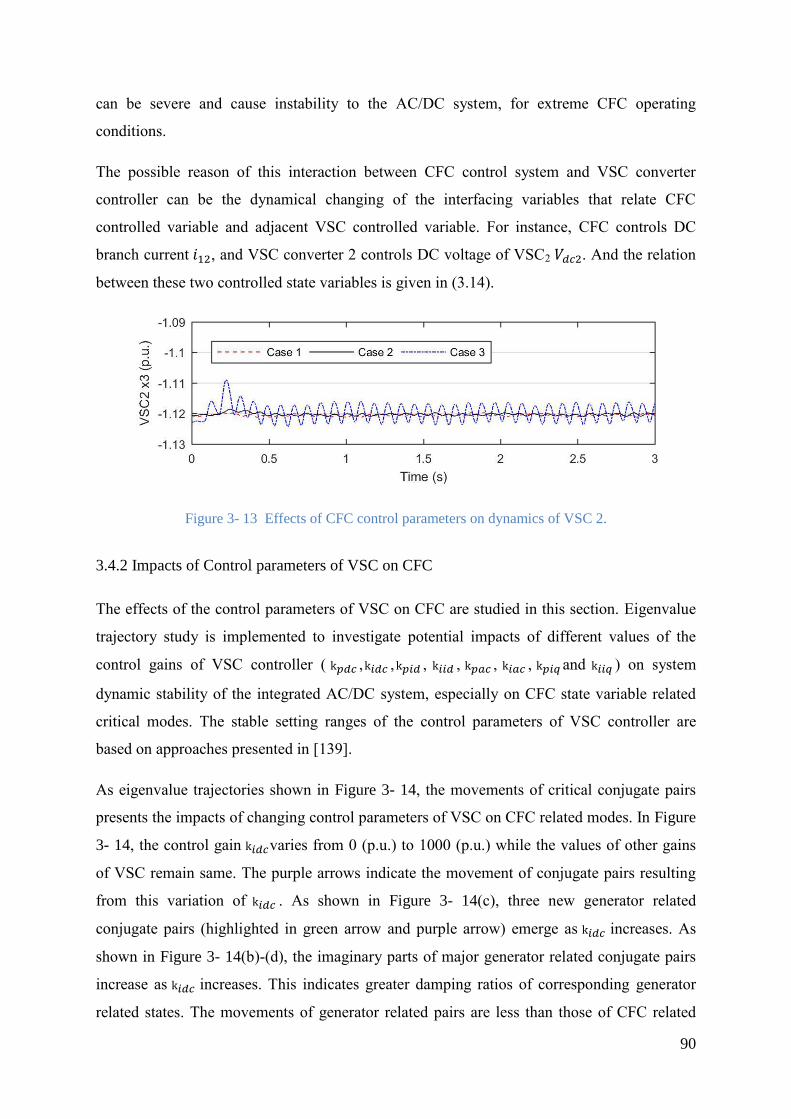
90

can be severe and cause instability to the AC/DC system, for extreme CFC operating

conditions.

The possible reason of this interaction between CFC control system and VSC converter

controller can be the dynamical changing of the interfacing variables that relate CFC

controlled variable and adjacent VSC controlled variable. For instance, CFC controls DC

branch current 𝑖 , and VSC converter 2 controls DC voltage of VSC2 𝑉𝑑𝑐 . And the relation

between these two controlled state variables is given in (3.14).

Figure 3- 13 Effects of CFC control parameters on dynamics of VSC 2.

3.4.2 Impacts of Control parameters of VSC on CFC

The effects of the control parameters of VSC on CFC are studied in this section. Eigenvalue

trajectory study is implemented to investigate potential impacts of different values of the

control gains of VSC controller ( k𝑝𝑑𝑐 ,k𝑖𝑑𝑐 ,k𝑝𝑖𝑑 , k𝑖𝑖𝑑 , k𝑝𝑎𝑐 , k𝑖𝑎𝑐 , k𝑝𝑖𝑞 and k𝑖𝑖𝑞 ) on system

dynamic stability of the integrated AC/DC system, especially on CFC state variable related

critical modes. The stable setting ranges of the control parameters of VSC controller are

based on approaches presented in [139].

As eigenvalue trajectories shown in Figure 3- 14, the movements of critical conjugate pairs

presents the impacts of changing control parameters of VSC on CFC related modes. In Figure

3- 14, the control gain k𝑖𝑑𝑐varies from 0 (p.u.) to 1000 (p.u.) while the values of other gains

of VSC remain same. The purple arrows indicate the movement of conjugate pairs resulting

from this variation of k𝑖𝑑𝑐 . As shown in Figure 3- 14(c), three new generator related

conjugate pairs (highlighted in green arrow and purple arrow) emerge as k𝑖𝑑𝑐 increases. As

shown in Figure 3- 14(b)-(d), the imaginary parts of major generator related conjugate pairs

increase as k𝑖𝑑𝑐 increases. This indicates greater damping ratios of corresponding generator

related states. The movements of generator related pairs are less than those of CFC related

91

and VSC related pairs as shown in Figure 3- 14(b) and (d). A new VSC 𝑥 related conjugate

pairs emerge as k𝑖𝑑𝑐 increases as shown in Figure 3- 14(d). The VSC related conjugate pairs

move towards left half of s-plane as k𝑖𝑑𝑐 increases, which indicates greater damping ratios of

VSC related states. It should be noted that positive eigenvalues are seen in Figure 3- 14(d).

This is due to the variation range of k𝑖𝑑𝑐 covers all stable and some points of unstable

operating range. As shown in Figure 3- 14(b) and (d), the movement of CFC related pairs

( 𝑖 , 𝑖 , and CFC 𝑦 ) clearly presents the impacts of VSC on CFC. The two conjugate pairs

of 𝑖 and 𝑖 move towards right half of s-plane which indicates reduced damping ratios of

CFC related states 𝑖 and 𝑖 . The conjugate pairs of CFC 𝑦 move towards left hand side

indicating increased damping ratios of CFC 𝑦 .

Based on eigenvalue trajectory studies of VSC control gains, it can be summarised that the

variation of VSC controller can affect dynamic stability of synchronous generator, VSC, and

CFC related modes. These impacts of VSC on CFC can result in different damping

characteristic of CFC related states, as VSC controller changes.

(a)

92

(b)

(c) (d)

Figure 3- 14 Eigenvalue trajectories of various VSC control parameter kidc.

As listed in Table 3- 10, two cases of different control parameters of VSC converter are

designed based on eigenvalue trajectories of various VSC control gains, to investigate their

effect on the CFC related system stability modes.

Case 4: control parameters (value of the gains of proportional and integral controllers) of

VSC2 are set to normal operating values ( 𝑘𝑝𝑑𝑐 = 7.52, k𝑝𝑎𝑐 = −10, 𝑘𝑝𝑖𝑑 = 0.3, 𝑘𝑝𝑖𝑞 =

0.3, 𝑘𝑖𝑑𝑐 = 1, 𝑘𝑖𝑎𝑐 = −1, 𝑘𝑖𝑖𝑑 = 1, and 𝑘𝑖𝑖𝑞 = 1) [139]. The system is stable.

Case 5: controller of VSC 2 is set to abnormal operating values ( 𝑘𝑝𝑑𝑐 = 7.52, 𝑘𝑝𝑎𝑐 =

−10, 𝑘𝑝𝑖𝑑 = 0.3, 𝑘𝑝𝑖𝑞 = 0.3, 𝑘𝑖𝑑𝑐 = 10, 𝑘𝑖𝑎𝑐 = −1000 𝑘𝑖𝑖𝑑 = 1, 𝑎𝑛𝑑 𝑘𝑖𝑖𝑞 = 1 ) which

represents extreme or possible fault VSC operating condition. One conjugate pair of

eigenvalues with positive real part can be seen which indicates small signal instability.

generator

𝑖 𝑖

𝑖 𝑖

VSCx

generator generator

CFC 𝑦 VSC x

93

Table 3- 10 Impacts of control parameters of VSC2 on CFC related modes

IMPACT OF CONTROL PARAMETERS OF VSC 2 ON DC CFC RELATED MODES

Related Eigenvalues Stability

Case 4 −0.09 ± j0.09(λ 9,40) stable

Case 5 0.52 ± j1.65(λ , 4) unstable, 1 positive pair of eigenvalues

Figure 3- 15 shows time-domain simulation results for the effects of control parameters of

VSC2 on dynamic performance of CFC. As shown in Figure 3- 15, a small perturbation (DC

branch current control reference i12 changes from 0.5 kA to 0.55 kA) is applied to CFC at

0.3s. For Case 4, i12 quickly increases to 0.55 kA in response to the change of reference. For

Case 5, large oscillations can be observed which indicates instability of CFC integrated DC

network.

Simulation results demonstrate that the VSC controller can affect the dynamic performance

of CFC. And this effect can be severe and cause instability of the CFC integrated DC network,

for extreme VSC operating conditions.

Figure 3- 15 Effect of control parameters of VSC converter 2 on DC CFC.

It should be pointed out here that the coordinated design of CFC control system and control

system of VSC can be carried out as future work in order to avoid possible negative

interactions between them.

3.5 Summary

In this chapter, DC network with CFC, including CFC and its control system has been

modelled in dynamic equations. The dynamic model of DC network with CFC has been

linearized and merged into VSC-based MTDC system without CFC presented in Chapter 2 to

formulate the state-space representation of multi-model system with CFC for small-signal

stability analysis. An integrated AC/DC system that consists of multiple synchronous

94

generators with excitation system and PSS, multiple VSC converters, and DC network with

CFC, has been established. Small-signal model of the test system has been derived based on

approaches presented in Chapter 2 and the eigenvalues of state-space representation of the

test system have been calculated. Modal analysis of calculated eigenvalues in comparison

between the integrated AC/DC system without/with CFC has been implemented to study the

impacts of incorporation of CFC, and its control parameters on small-signal stability of the

integrated AC/DC system.

It can be found from eigenvalue results that all 55 eigenvalues have non-positive real part.

This indicates a stable operating condition at the considered operating point. There are two

zero eigenvalues, as there is no infinite busbar in the testing network. One of the eigenvalue



because mechanical damping is neglected and governor action is not represented. If the rotor

angle and angular velocity of one synchronous machine are regarded as references, and the

governor action of mechanical damping is considered, the two zero eigenvalues will be

reduced. Compared to eigenvalue results of AC/DC system without CFC, there is no

significant changes of values of synchronous generator related conjugate pairs caused by the

incorporation of CFC. This indicates that the corporation of CFC has no significant impacts

on dynamic stability of multi synchronous generators.

The conjugate pairs which are related to the dominant state variables of DC networks with

CFC are seen, according to their participation factors. The dominant states of these conjugate

pairs are CFC controlled state variables. These results indicate that the incorporation of CFC

causes the emergence of CFC related eigenvalues, hence the oscillations of relevant DC

network states are expected. It should be noted that the VSC related conjugate pairs is seen,

which indicates that the incorporation of CFC can even results in the emergence of VSC

related eigenvalues. The dynamic stability of VSC is affected by the integration of CFC. An

approach of determining stable/unstable setting ranges of control parameters of CFC is

presented and validated by simulation results in RTDS/RSCAD. The simulation results

demonstrate that the control parameters of CFC may cause instability of the system if they

are not carefully-tuned.

Simulations results of established AC/DC system against disturbances are in line with the

modal analysis results, since stable operating condition around operating point is seen from

95

simulation results in RTDS/RSCAD against both small disturbance of change of reference

and large disturbances (including AC system faults, and DC cable faults).

Based on eigenvalue trajectory studies of CFC control gains, it can be summarised that the

variation of CFC controller can affect dynamic stability of CFC and VSC related modes.

These impacts of CFC on VSC can result in different damping characteristics of VSC related

states, as CFC controller changes. This effect can be severe and cause instability to the

AC/DC system, for extreme CFC operating conditions. And it can also be found that the

variation of VSC controller can affect dynamic stability of synchronous generators, VSC, and

CFC related modes, based on eigenvalue trajectory studies of VSC control gains. These

impacts can result in different damping characteristics of CFC related states, as VSC

controller changes. And this effect can be negative and cause instability of the CFC

integrated DC network, for extreme VSC operating conditions. It should be pointed out here

that the coordinated design of CFC control system and control system of VSCs can be carried

out as future work in order to avoid possible negative interactions between them.

96

CHAPTER 4 IMPACTS OF VSC HVDC SYSTEM ON

DISTANCE PROTECTION

4.1 Introduction

This chapter investigates the impacts of the integration of VSC HVDC system on HV feeder

distance protection. The mathematical representation of the apparent impedance

measurements of distance relays is presented considering the infeed current from VSC

HVDC system connected busbar. Relevant analysis of the apparent impedance measurement

representation and dynamic simulation study is conducted to investigate the impacts of VSC

HVDC system on distance protection. In 4.2, a typical feeder distance protection of two-

ended overhead transmission lines is reviewed, including basic principles of distance

protection, zones of protection, distance relay characteristics, and under-reach and overreach

effect of distance relay application. In 4.3, mathematical representation of the apparent

impedance measurement of distance relay for zone 2 protection is derived considering infeed

current from VSC HVDC connected busbar. A RTDS-based hardware in the loop (HIL)

testing platform is established to perform dynamic simulation studies of test system with

VSC HVDC. The dynamic simulation results are analysed in comparison between the test

system without/with VSC HVDC.

4.2 Distance Protection of Two-Ended Overhead Transmission Lines

Normal application of distance protection of two-ended overhead transmission lines is

presented in this section, including basic principles, zones of protection, residual

compensation, and under-reach and overreach effect.

4.2.1 Basic Principles of Distance Protection

Distance protection is a kind of economic and fast-reacted non-unit system of protection.

Distance relays use measurements of line voltages and line currents from protected area to

calculate apparent impedance. The impedance of HV and extra high voltage (EHV)

transmission lines is usually proportional to the line length. In consequence, it is possible to

97

determine if a fault occurs in the protection zone or out of protection zone by comparing the

calculated impedance to the protected line impedance [93].

Distance protection is considered to be simple to apply and fast in operation for faults located

along most of a protected circuit. It is suitable for application with high-speed auto-reclosing.

As single-line diagram of distance protection shown in Figure 4- 1, the measured apparent

impedance by distance relay is independent of the source impedance which can be derived as

follows:

𝐼𝑓𝑎𝑢𝑙𝑡 =𝑉𝑠𝑜𝑢𝑟𝑐𝑒

𝑍𝑠𝑜𝑢𝑟𝑐𝑒+𝑍𝑙𝑖𝑛𝑒𝑎 (4. 1)

𝐼𝑟𝑒𝑙𝑎𝑦 = 𝐼𝑓𝑎𝑢𝑙𝑡 (4. 2)

𝑉𝑟𝑒𝑙𝑎𝑦 = 𝐼𝑓𝑎𝑢𝑙𝑡 × 𝑍𝑙𝑖𝑛𝑒𝑎 (4. 3)

𝑍𝑟𝑒𝑙𝑎𝑦 =𝑉𝑟𝑒𝑙𝑎𝑦

𝐼𝑟𝑒𝑙𝑎𝑦= 𝑍𝑙𝑖𝑛𝑒𝑎 (4. 4)

Vsource

Zsource Zlinea Zlineb

Distance

Relay

faultIrelay

Vrelay

Ifault

Figure 4- 1 Single-line diagram of distance protection.

Distance relays are designed to operate only when faults occurred are within the protection

zone, which is the protection range between the relay location and the selected reach point.

The calculated apparent impedance is compared with the reach point impedance. If the

calculated apparent impedance is less than the reach point impedance, it is assumed that a

fault occurs on the line between the relay and the reach point. The distance relay operates and

sends signals to related circuit breakers and circuit breakers trip. If the calculated apparent

impedance is greater than the reach point impedance, it is assumed that no fault occurs on the

line between the relay and the reach point. Once the settings of distance relay are determined

the protection is relatively unaffected by changes in the power system.

98

The reach point of a distance relay is a certain point along the line impedance locus which

indicates the boundary of protection. The reach point can be plotted on an R/X diagram since

it is dependent on the ratio of voltage and current and phase angle between them.

The major advantages of distance protection are as follows [93]:

1. High-speed of operation.

2. Ability to protect independent of communication services.

And the major disadvantages of distance protection are considered to be as follows [93]:

1. Need of both CTs and VTs.

2. Limited resistive fault coverage.

4.2.2 Zones of Protection

The reach settings and tripping times for various zones of protection should be carefully

selected so that correct coordination between multiple distances relays on power system are

achieved. Basic distance protection consists of instantaneous Zone 1 protection and one or

more time-delayed zones. The protection zones studied in this thesis are Zone 1 protection

and Zone 2 protection.

Conventional electromechanical/ static relays usually use a reach setting of up to 80% of the

protected line impedance for instantaneous Zone 1 protection. Digital/numerical distance

relays may use settings of up to 85% to be safe. The 15%-20% safety margin ensures no risk

of over-reaching effect in Zone 1 protection, due to errors in the current and voltage

measurement of coupling transformers, inaccuracies in line impedance data and errors of

relay settings. The relay setting for Zone 1 protection in this study is 75% of the line

impedance, which is in line with the Grid Code of UK.

The reach settings of the Zone 2 protection is usually at least 120% of the protected line

impedance to ensure that full length of line is covered with allowance for the sources of error

as listed for Zone 1 protection. The relay settings for Zone 2 protection in this study is 150%

of the line impedance, which is in line with the Grid Code of UK so that the full protection

range of Zone 1 and Zone 2 protection of a distance relay overlaps the protection range of

Zone 1 protection of the remote end distance relay located at adjacent transmission line.

99

The tripping of Zone 2 protection should be time-delayed so that the Zone 1 protection of

remote relay can operates first. Thus complete length of a transmission line is covered with

fast clearance of faults in the first 80-85% of the line and slower clearance of faults in the

remaining section of the line. Other protection zones for additional protection proposes are

not considered in this study.

4.2.3 Distance Relay Characteristics

Plain impedance characteristic of distance relay which takes no account of the phase angle

between the current and voltage applied to it is considered in this study. The calculated

impedance is a circle with its centre at the origin of the coordinates and radius equal to its

setting in ohms when plotted on an R/X diagram. The distance relay operates if the calculated

impedance is less than setting value, that is, for all points within in the circle in R/X diagram.

This relay characteristic is non-directional.

As for distance relay located near bus A (the distance between distance relay and bus A can

be neglected) protecting line AB shown in Figure 4- 2, the plain impedance relay

characteristic is shown is Figure 4- 3. The segment AB in R/X diagram represents the

complete line impedance of transmission line AB. The parameters of transmission line AC

and AB can be considered same as an example. Hence, the segment AC represents the

complete line impedance of transmission line AC. The green circle in R/X diagram represents

the impedance locus of fault occurred in protection Zone 1, which is 75% of the complete

length of line AB. The radius of circle Zone 1 is 75% of segment AB. Similarly, the blue

circle in R/X diagram represents the impedance locus of fault occurred in protection Zone 2,

which is 150% of the complete length of line AB. The radius of circle Zone 2 is 150% of

segment AB. For any fault with impedance locus within the circle of Zone 1 and Zone 2, the

distance relay operates and sends trip signals to related circuit breakers. For any fault with

impedance locus without the circle Zone 2, the distance relay restraints. This protection range

covers the whole length of line AB and even adjacent transmission lines (for example AC in

this case).

100

Zlineab

Distance

Relay

Irelay

Vrelay

Zlineac

A BC

Figure 4- 2 Single-line diagram of distance protection located at two adjacent lines.

A

B

C

Restrains

Operates

R

X

Zone 1 Zone 2

Figure 4- 3 Plain impedance relay characteristic.

It should also be noted that the plain impedance relay characteristic has disadvantages. It is

non-directional which means it reacts to faults both in front of and behind the relaying point.

For unbalanced and line to ground faults, the voltage and current measurements of a

particular phase should be compensated to ensure correct measured quantities are used.

Distance relays compare positive sequence apparent impedance from measurements to those

from line data. But for unbalanced and earth faults, the measurements of line voltage and

101

current are not in positive sequence and should be compensated with residual compensation

factor. Considering phase A to ground fault as an example to study, the voltage drop to the

fault and current in the fault loop can be expressed as follows:

𝑉𝑎 = 𝐼 𝑍𝐿 + 𝐼 𝑍𝐿 + 𝐼0𝑍𝐿0 (4. 5)

𝐼𝑎 = 𝐼 + 𝐼 + 𝐼0 (4. 6)

where

𝑉𝑎 and 𝐼𝑎 : voltage and current of phase a measured by distance relay

𝐼 , 𝐼 , and 𝐼0 : positive, negative and zero sequence current through transmission line

𝑍𝐿 , 𝑍𝐿 , and 𝑍𝐿0: positive, negative and zero sequence impedance from fault point

The line positive and negative sequence impedances are assumed equal (𝑍𝐿 =𝑍𝐿 ). And the

zero sequence current can be expressed as follows:

𝐼𝑎 + 𝐼𝑏 + 𝐼𝑐 = 3𝐼0 (4. 7)

where

𝐼𝑏 and 𝐼𝑐 : phase current of phase b and c at relaying point

(4.5) can be simplified by substituting (4.6) and (4.7) as follows:

𝑉𝑎 = 𝑍𝐿 (𝐼𝑎 + 𝐼0𝑍𝐿0−𝑍𝐿1

𝑍𝐿1) (4. 8)

The residual compensation factor 𝐾𝑍0 is defined as follows:

𝐾𝑍0 =𝑍𝐿0−𝑍𝐿1

𝑍𝐿1 (4. 9)

(4.8) can be simplified as follows by substituting (4.9):

𝑉𝑎 = 𝑍𝐿 (𝐼𝑎 + 3𝐼0𝐾𝑍0) (4. 10)

𝑍𝐿 =𝑉𝑎

𝐼𝑎+ 𝐼0𝐾𝑍0 (4. 11)

In this case, the relationship between 𝐼𝑎 and 𝐼0 can be expressed as follows:

𝐼𝑎 = 3𝐼0 (4. 12)

102

(4.11) can be simplified as follows by substituting (4.12):

𝑍𝐿 =𝑉𝑎

𝐼𝑎( +𝐾𝑍0) (4. 13)

In this way, the correct positive sequence apparent impedance from fault location can be

calculated by use of phase voltage and current measurement compensated with residual

compensated factor.

4.2.4 Under-reach and Over-reach Effect of Distance Relay Application

A number of various problems might be encountered in application of distance relays. The

major problems that are likely to happen are under-reach and over-reach effect. These

unwanted effects of distance relays should be made aware of to avoid consequent mal-

operations.

The under-reach is defined as that the measured apparent impedance by distance relay is

greater than the real impedance to the fault [93]. And the percentage under-reach is defined as

follows:

𝑍𝑅−𝑍𝑀

𝑍𝑅× 100% (4. 14)

where

𝑍𝑅 : intended relay reach (relay reach setting)

𝑍𝑀 : measured reach

The main cause of under-reach is the fault current infeed at remote busbars which is shown in

Figure 4- 4. For fault occurred at point C, the measured apparent impedance is not 𝑍𝑎 + 𝑍𝑐

due to the infeed current 𝐼𝑏. The measured apparent impedance is calculated by distance relay

as follows:

𝑍𝑀 = 𝑍𝑎 + 𝑍𝑐𝐼𝑎+𝐼𝑏

𝐼𝑎 (4. 15)

where

𝑍𝑎 and 𝑍𝑐 : line impedance of line AB and line BC

𝐼𝑎 and 𝐼𝑏 : line current of line AB and line BD

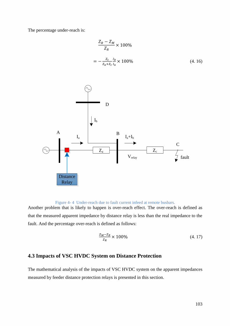
103

The percentage under-reach is:

𝑍𝑅 − 𝑍𝑀

𝑍𝑅× 100%

= −𝑍𝑐

𝑍𝑎+𝑍𝑐

𝐼𝑏

𝐼𝑎× 100% (4. 16)

Zc

Distance

Relay

Ia

Vrelay

Za

A B

C

fault

Ib

Ia+Ib

D

Figure 4- 4 Under-reach due to fault current infeed at remote busbars.

Another problem that is likely to happen is over-reach effect. The over-reach is defined as

that the measured apparent impedance by distance relay is less than the real impedance to the

fault. And the percentage over-reach is defined as follows:

𝑍𝑀−𝑍𝑅

𝑍𝑅× 100% (4. 17)

4.3 Impacts of VSC HVDC System on Distance Protection

The mathematical analysis of the impacts of VSC HVDC system on the apparent impedances

measured by feeder distance protection relays is presented in this section.

104

Figure 4- 5 shows the simplified single line diagram of a faulted network for the analysis of

impacts of VSC HVDC system. Two AC systems (represented by ideal voltage source with

internal impedance) are connected via double-circuit transmission lines TL1 and TL2. The

line parameters for the double circuits of same transmission line are same. A VSC converter

is connected near B2 (the distance between VSC converter and B2 can be neglected) to

provide voltage support and active power transmission. Two distance relays (Distance relay 1

and Distance relay 2) are located at the both ends of one single-circuit of TL1. These distance

relays collect voltage and current measurements from voltage transformer (VT) and current

transformer (CT) and send trip signals to circuit breakers (CB1 and CB2). An external single-

phase-to-ground (SLG) fault or three-phase fault on TL2 occurs at p% of the full length of

TL2 from B2.

TL1 TL2

B1

CB1 CB2

Distance

Relay 1

Distance

Relay 2

B2 B3

VSC

HVDC

ZL

IVSC

Is

If

Rf

pZ’L

VLVR

I’s (1-p)Z’L

I’’

s

Figure 4- 5 Simplified SLD of a faulted network for the analysis of impacts of VSC system.

The distance protection used on TL1 applies the normal protection scheme that is presented

in 4.2. Two distance relays, Distance relay 1 and Distance relay 2 are set to use Zone 1 and

Zone 2 protection. The relay settings for Zone 1 protection is 75% of the line impedance. The

relay settings for Zone 2 protection is 150% of the line impedance so that the full protection

range of Zone 1 and Zone 2 protection of a distance relay covers the full length of

transmission line. Plain impedance characteristic of distance relay is considered in this study.

The VSC converter connected at B2 is modelled as that presented in Chapter 2. The control

mode of VSC control system can be set to DC voltage regulation or active power transfer

control for d axis, and AC voltage regulation or reactive power control for q axis.

105

Considering the fact that VSC HVDC is normally connected to busbars, the impacts of VSC

HVDC system are mainly on Zone 2 protection. This is because the current infeed from VSC

HVDC is without the protection range of Zone 1 protection but it is within the protection

range of Zone 2 protection. Hence the distance protection against internal fault of TL1 is not

affected by the incorporation of VSC, but the external fault located at TL2 is affected by the

incorporation of VSC HVDC.

The apparent impedance of VSC-connected transmission line measured by distance relay is

derived for SLG faults and three-phase faults to investigate the impacts of VSC HVDC

system on distance protection.

For SLG faults, the voltages seen by VT at B1 can be expressed as follows:

𝑉𝐿𝑥 = 𝑍𝐿𝑥𝐼𝑠𝑥 + 𝑝𝑍𝐿𝑥′ 𝐼𝑠𝑥

′ + 𝐼𝑓𝑥𝑅𝑓 (4. 18)

for 𝑥 = 1,2, 𝑜𝑟 0 as a suffix denote of the sequence components, where

𝑉𝐿𝑥 : sequence voltages seen by VT at B1

𝐼𝑠𝑥 : sequence currents seen by CT at B1

𝐼′𝑠𝑥 : sequence phase current through faulted single-circuit of TL2 from B2 to B3

𝐼𝑓𝑥 : sequence current through fault resistance

𝑅𝑓 : fault resistance

𝑍𝐿𝑥and 𝑍𝐿𝑥′ : sequence components of the line impedance of TL1 and TL2.

𝑝 : fault location from B2 to B3 in per unit of the total line length

The line positive and negative sequence impedances are assumed equal.

𝑍𝐿 = 𝑍𝐿 , 𝑍𝐿 ′ = 𝑍𝐿

′ (4. 19)

By adding all three sequence components of left-hand side of (4.18) and substitute (4.19) into

(4.18), the voltages seen by VT can be expressed after simplification as follows:

𝑉𝐿 = 𝑍𝐿 (𝐼𝑠 + 𝑘𝐼𝑠0) + 𝑝𝑍𝐿𝑥′ (𝐼𝑠

′ + 𝑘′𝐼𝑠0′ ) + 𝐼𝑓𝑅𝑓 (4. 20)

where

106

𝑉𝐿and 𝐼𝑠 : phase voltage and current of faulted phase through TL1

𝐼𝑠′ : phase current of faulted phase through faulted single-circuit of TL2 from B2 to B3

𝐼𝑓 : fault current through fault resistance

𝑘 : zero sequence current compensation factors of TL1

𝑘′ : zero sequence current compensation factors of TL2

𝑘 =𝑍𝐿0 − 𝑍𝐿

𝑍𝐿 (4. 21)

𝑘′ =𝑍𝐿0

′ − 𝑍𝐿 ′

𝑍𝐿 ′ (4. 22)

For transient response study of double-circuit transmission line, the fault currents through the

double circuits of TL1 can be assumed to be equal due to the line parameters of double

circuits are same. Hence, by use of KCL law to B2, the relationship of inflow currents and

outflow currents can be expressed as follows:

2𝐼𝑠 + 𝐼𝑉𝑆𝐶 = 𝐼𝑆′ + 𝐼𝑆

′′ (4. 23)

where

𝐼𝑉𝑆𝐶 : phase current infeed from VSC HVDC

𝐼𝑆′′ : phase current of faulted phase through unfaulted single-circuit of TL2 from B2 to B3

By substitute (4.23) into (4.20), the voltages seen by VT can be expressed as follows:

𝑉𝐿 = 𝑍𝐿 (𝐼𝑠 + 𝑘𝐼𝑠0) + 𝑝𝑍𝐿𝑥′ [2𝐼𝑠 + 𝐼𝑉𝑆𝐶 − 𝐼𝑆

′′ + 𝑘′(2𝐼𝑠0 + 𝐼𝑉𝑆𝐶0 − 𝐼𝑆0′′ )] + 𝐼𝑓𝑅𝑓 (4. 24)

By use of delta connection at one side of the coupling transformer of VSC converter, the

zero-sequence current injection can be eliminated [155]. Hence the zero-sequence current of

VSC is eliminated.

𝐼𝑉𝑆𝐶0 = 0 (4. 25)


107

𝑉𝐿 = 𝑍𝐿 (𝐼𝑠 + 𝑘𝐼𝑠0) + 𝑝𝑍𝐿𝑥′ [2𝐼𝑠 + 𝐼𝑉𝑆𝐶 − 𝐼𝑆

′′ + 𝑘′(2𝐼𝑠0 − 𝐼𝑆0′′ )] + 𝐼𝑓𝑅𝑓 (4. 26)

By use of phase voltage measurements at B1 ( 𝑉𝐿 ) and phase current measurement

compensated by zero sequence current (𝐼𝐿), the apparent impedance seen by the Distance

relay 1 are given as:

𝑍𝑟𝑒𝑙𝑎𝑦 =𝑉𝐿

𝐼𝐿= 𝑍𝐿 + 𝑝𝑍𝐿

′2𝐼𝑠 + 𝐼𝑉𝑆𝐶 − 𝐼𝑆

′′ + 𝑘′(2𝐼𝑠0 − 𝐼𝑆0′′ )

𝐼𝑠 + 𝑘𝐼𝑠0+

𝐼𝑓

𝐼𝐿𝑅𝑓

= 𝑍𝐿 + 𝑝𝑍𝐿 ′

2𝐼𝑠 − 𝐼𝑆′′ + 𝑘′(2𝐼𝑠0 − 𝐼𝑆0

′′ )

𝐼𝑠 + 𝑘𝐼𝑠0+ 𝑝𝑍𝐿

′𝐼𝑉𝑆𝐶


𝐼𝑓

𝐼𝐿𝑅𝑓 (4. 27)

𝐼𝐿 = 𝐼𝑠 + 𝑘𝐼𝑠0 (4. 28)

where

𝑍𝑟𝑒𝑙𝑎𝑦 : apparent impedance measured Distance relay 1

𝐼𝐿 : compensated phase current of faulted phase measure by Distance relay 1

For three-phase faults, the phase current seen by distance relay is as follows:

𝐼𝐿 = 𝐼𝑠 + 𝑘𝐼𝑠0 = 𝐼𝑠 (4. 29)

𝐼𝑠 = 𝐼𝑠0 = 0 (4. 30)

𝐼𝑠 ′ = 𝐼𝑠0

′ = 0 (4. 31)

Similarly, the apparent impedance seen by the distance relay is given as follows:



′2𝐼𝑠 + 𝐼𝑉𝑆𝐶 − 𝐼𝑆

′′

𝐼𝑠+

𝐼𝑓

𝐼𝐿𝑅𝑓

= 𝑍𝐿 + 𝑝𝑍𝐿 ′ 𝐼𝑠−𝐼𝑆

′′

𝐼𝑠+ 𝑝𝑍𝐿

′ 𝐼𝑉𝑆𝐶

𝐼𝑠+

𝐼𝑓

𝐼𝐿𝑅𝑓 (4. 32)

By carefully looking into (4.27) and (4.32), the VSC’s impacts on the apparent impedance

measured by Distance relay 1 in case of external fault can be summarised as:

1. The first and second terms (𝑍𝐿 + 𝑝𝑍𝐿 ′ 𝐼𝑠−𝐼𝑆

′′+𝑘′( 𝐼𝑠0−𝐼𝑆0′′ )

𝐼𝑠+𝑘𝐼𝑠0 and 𝑍𝐿 + 𝑝𝑍𝐿

′ 𝐼𝑠−𝐼𝑆′′

𝐼𝑠) of (4.27)

and (4.32) represent the actual line impedance of TL1 and proportional line impedance of

108

TL2 to the fault location. The fourth term (𝐼𝑓

𝐼𝐿𝑅𝑓) represents the contribution of fault

resistance. These terms (the first, second and fourth) are not affected by the integration of

VSC HVDC.

2. The third terms (𝑝𝑍𝐿 ′ 𝐼𝑉𝑆𝐶

𝐼𝐿) of (4.27) and (4.32) indicates that the VSC HVDC’s impacts

on the apparent impedance measured by Distance relay 1 against external fault lead to

greater apparent impedance measurement. The under-reach effect is introduced as the

impacts of VSC HVDC. Since during external fault, the VSC is injecting reactive power

and current to support bus voltage, the apparent impedance is greater than test system

with no VSC HVDC. For steady state, while VSC HVDC is absorbing reactive power

and current from bus bar, the third term could be negative. This negative value indicates

less apparent impedance of connected TL1, which results in overreach effect as the

impacts of VSC HVDC. This error in apparent impedance measurements caused by VSC

HVDC is proportional to the current ratio of VSC HVDC and relay, and fault location.

4.4 Dynamic Simulation Study

4.4.1 Establishment of RTDS-based Hardware-in-Loop Testing Platform

A RTDS-based HIL testing platform for protective relay studies proposed in [168] is

established as shown in Figure 4- 6. Digital signals are generated from RTDS, and converted

into analogue signals via Giga-Transceiver Analogue Output (GTAO) card. The output

analogue signals are amplified by power amplifier for practical distance protective relays.

The trip signals are sent back from the protective relays to RTDS via the front panel to

control the operations of circuit breakers. Identical network topology described in 4.3 is used

for external fault test. The transmission line parameters and equivalent voltage source

parameters are listed in Appendix B.1 and B.2.

As listed in Appendix B.2, the voltage level of equivalent voltage source is set based on

transmission data from the Electricity Ten Year Statement (ETYS) published annually by

National Grid UK. The internal impedance parameters at each end of transmission lines are

set based on fault level data from the ETYS. As listed in Appendix B.1, the transmission line

parameters are set based on transmission line data from the ETYS.

109

2 × 3-

Phase

Current

Signals;

2 × 3-Phase

Voltage Signals;

3-Ph I2

D/A

Conversion

3-Ph V2

TL1 TL2

B1RTDS/RSCAD

3-Ph I1

3-PhV1

3-Ph V1 3-Ph V1

3-Ph I13-Ph I1

3-Ph V2

3-Ph I2 3-Ph I2

CB1 CB2

Amplifier 1Distance Relay 1


Physical Devices

B2 B3

3-Ph V2

Physical Devices

Digital

Output

VSC

Figure 4- 6 RTDS-base HIL testing platform for VSC HVDC studies.

4.4.2 Test System with VSC HVDC and Protection Relay Settings

The schematic diagram of the trial network is illustrated in Figure 4- 6. There is one GE

MiCOM P40 Agile P443 distance relay located at each end of two-ended transmission lines

from B1 to B2, measuring the local current and voltage signals. In this thesis,

communications between relays are not considered.

Figure 4- 6 shows the arrangements of VT, CT and CB for one of the aforementioned series

compensated lines between B1 and B2. Distance protection using GE MiCOM P40 Agile

P443 distance protection relays is used. Two VTs and two CTs at both ends of the

transmission line provide voltage and current measurements. The transmission line

parameters and equivalent voltage source parameters are listed in Appendix B.1 and B.2.

The following considerations are taken into account for the settings of the 2-ended distance

protections:

1. Zone 1 is set to 75% of the complete circuit positive sequence impedance. The tripping

delay is set to 0ms.

2. Zone 2 is set to reach 150% of the complete circuit positive sequence impedance. The

tripping delay is set to 500ms.

110

4.4.3 Dynamic Simulation Result of Test System without/with VSC HVDC

External faults occur at one single-circuit of TL2 from B2 to B3 under such fault conditions:

1. 600ms fault occurred at 105% and 135% of the equivalent whole length of TL1.

2. Fault resistance is 0.01Ω, and 1 Ω.

3. SLG, and three-phase to ground faults are considered.

Table 4- 1 shows the simulation results of external fault. The tripped zone is noted as “I”, “II”,

or “X” for Zone 1, Zone 2 or no relay operation is seen, respectively. Fault type is noted as

“RYB-G”, or “R-G” for three-phase to ground, or SLG faults, respectively.

Table 4- 1 Simulation results for test system without/with VSC HVDC against external fault

Case Fault

Location

Fault

Impedance

Fault

Type

Fault

Duration

Distance relay 1

No VSC

VSC

1 105% 0.01Ω RYB-G 600ms II

105.6%

II

107.6%

2 105% 0.01Ω R-G 600ms II

106.1%

II

108.2%

3 105% 1Ω RYB-G 600ms II

106.0%

II

108.3%

4 105% 1Ω R-G 600ms II

106.6%

II

108.8%

5 135% 0.01Ω RYB-G 600ms II

136.4%

II

143.1%

6 135% 0.01Ω R-G 600ms × ×

7 135% 1Ω RYB-G 600ms × ×

8 135% 1Ω R-G 600ms × ×

Figure 4- 7 shows digital signals from RSCAD for a typical external fault Case 1 of Table 4-

1 with no VSC HVDC integration, and Figure 4- 7 shows the trajectory of impedance

measurements by distance relay during fault. Figure 4- 8 shows digital signals from RSCAD

for a typical external fault Case 1 of Table 4- 1 with VSC HVDC, and Figure 4- 8 shows the

corresponding trajectory of impedance measurements by distance relay.

111

As shown in Figure 4- 8, VT and CT send voltage and current measurements (noted as

VA/VB/VC and IA/IB/IC) to distance relay. By use of the received measurements and

impedance calculation algorithm presented in 4.3, the apparent impedance is calculated

(noted as ZIM vs ZRE in Figure 4- 8). The trip signals (noted as TripA/TripB/TripC in Figure

4- 8) are sent to corresponding CBs, by judgement if calculated apparent impedance is within

protection zones. The CBs are turn off or turn on (noted as CBA/CBB/CBC in Figure 4- 8),

controlled by received trip signals.

By comparison of the apparent impedances measured by distance relay, the apparent

impedance with VSC is greater than impedance with no VSC HVDC integration. The under-

reach effect of distance relay is seen due to the incorporation of VSC HVDC.

Figure 4- 7 Digital signals from RSCAD for test system without VSC HVDC in Case 1.

112

Figure 4- 8 Digital signals from RSCAD for test system with VSC HVDC in Case 1.

Figure 4- 9 shows digital signals from RSCAD for a SLG external fault Case 2 of Table 4- 1

with VSC HVDC.

As voltage and current measurement of VT and CT (noted as VA/VB/VC and IA/IB/IC)

shown in Figure 4- 9, SLG fault occurred. The three-phase trip signals (noted as

TripA/TripB/TripC) are sent to corresponding CBs. This is due to the fact that distance relay

settings require relays trip all three phases for Zone 2 protection.

Figure 4- 9 Digital signals from RSCAD for test system with VSC HVDC in Case 2.

Figure 4- 10 shows digital signals from RSCAD for a 1 Ω external fault Case 3 of Table 4- 1

with VSC HVDC integration, and Figure 4- 10 shows the trajectory of impedance

measurement by distance relay. By comparison of the apparent impedances measured by

distance relay, the apparent impedance against 1 Ω fault is greater than impedance against

113

0.01 Ω. These results are in line with the conclusion in 4.3 that the error of measured

impedance is positively related to fault resistance.

Figure 4- 10 Digital signals from RSCAD for a 1 Ω external fault Case 3.

Figure 4- 11 shows digital signals from RSCAD for a 135% external fault Case 7 of Table 4-

1 with VSC HVDC integration, and Figure 4- 11 shows the trajectory of impedance

measurement by distance relay. It can be seen from Figure 4- 11 that the distance relay is not

tripped if the fault distance is too far. By comparison of the apparent impedances measured

by distance relay, the apparent impedance against 135% fault is greater than impedance

against 105% fault. These results are in line with the conclusion in 4.3 that the error of

measured impedance is positively related to fault distance.

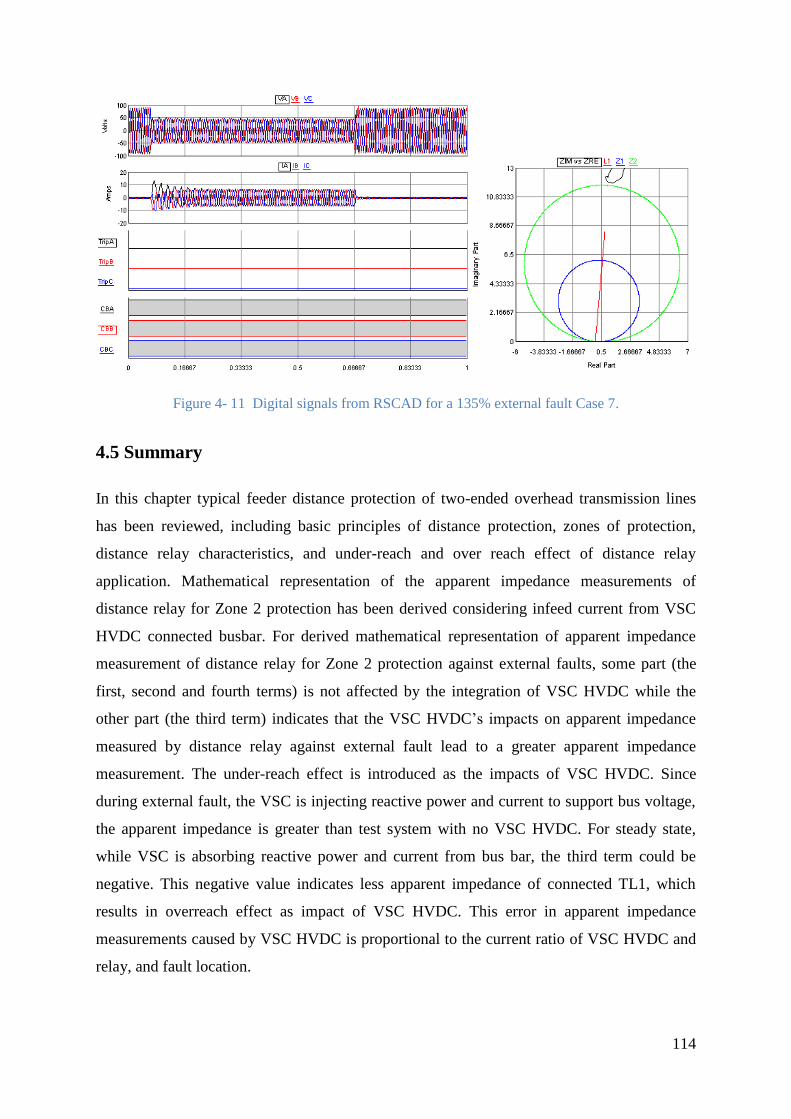
114

Figure 4- 11 Digital signals from RSCAD for a 135% external fault Case 7.

4.5 Summary

In this chapter typical feeder distance protection of two-ended overhead transmission lines

has been reviewed, including basic principles of distance protection, zones of protection,

distance relay characteristics, and under-reach and over reach effect of distance relay

application. Mathematical representation of the apparent impedance measurements of

distance relay for Zone 2 protection has been derived considering infeed current from VSC

HVDC connected busbar. For derived mathematical representation of apparent impedance

measurement of distance relay for Zone 2 protection against external faults, some part (the

first, second and fourth terms) is not affected by the integration of VSC HVDC while the

other part (the third term) indicates that the VSC HVDC’s impacts on apparent impedance

measured by distance relay against external fault lead to a greater apparent impedance

measurement. The under-reach effect is introduced as the impacts of VSC HVDC. Since

during external fault, the VSC is injecting reactive power and current to support bus voltage,

the apparent impedance is greater than test system with no VSC HVDC. For steady state,

while VSC is absorbing reactive power and current from bus bar, the third term could be

negative. This negative value indicates less apparent impedance of connected TL1, which

results in overreach effect as impact of VSC HVDC. This error in apparent impedance

measurements caused by VSC HVDC is proportional to the current ratio of VSC HVDC and

relay, and fault location.

115

As shown in dynamic simulation results in RTDS/RSCAD, the apparent impedance with

VSC HVDC is greater than impedance with no VSC HVDC integration, by comparison of

the apparent impedances measured by distance relay. The under-reach effect of distance relay

is seen due to the incorporation of VSC HVDC. The dynamic simulation results are in line

with mathematical analysis presented in 4.3, considering the results that the error of measured

impedance is positively related to fault resistance, and fault distance.

116

CHAPTER 5 IMPACTS OF VSC FACTS ON

DISTANCE PROTECTION

5.1 Introduction

This chapter presents the mathematical representation of the apparent impedance

measurements of distance relay considering the infeed current from shunt VSC FACTS (in

particular, STATCOM as a typical example) connected busbar. Relevant analysis of the

apparent impedance measurement representation and dynamic simulation study is

implemented to investigate the impacts of VSC FACTS on distance protection. In 5.2,

dynamic representation of STATCOM is modelled considering its configuration and control

system. In 5.3, mathematical representations of the apparent impedance measurements of

neighbouring and remote distance relays against internal and external faults are derived

considering infeed current from STATCOM connected at different busbars. A RTDS-based

HIL testing platform is established to perform dynamic simulation studies of test system with

STATCOM. The dynamic simulation results are analysed in comparison between test system

without/with STATCOM at different locations against internal and external faults.

5.2 Modelling of STATCOM

The modelling of detailed delta-connected MMC based STATCOM is presented in this

section, comprising of configuration, and control system.

5.2.1 Configuration of STATCOM

A static synchronous compensator (STATCOM), or static synchronous condenser

(STATCON), is a VSC-based power electronics regulating system integrated to AC power

transmission system. It is used to regulate AC voltage or provide reactive AC power to the

connected power network. It is a commonly used shunt device of FACTS family and a typical

example of shunt VSC FACTS to study in this thesis.

As the same with VSC HVDC, there a number of various topologies of STATCOM in

different voltage levels, since the converter of STATCOM is VSC based. These topologies

vary in different voltage levels, depending on different application scenarios: two-level

117

converter, three-level converter, or multilevel modular converter. As for the connection

topologies for converter legs, unlike VSC HVDC, there are two connections for converter

legs for STATCOM, star-connection and delta-connection. Figure 5- 1 shows the topology of

a star-connected STATCOM which shares the same VSC converter topology of VSC-HVDC

system as reviewed in 2.2, only except that the DC side of STATCOM is a DC storage

capacitor rather than DC link to DC network.

to AC System

+

-

DC side

Figure 5- 1 Topology of a star-connected STATCOM.

The three-phase circuit configuration of the delta-connection MMC-based STATCOM is

shown in Figure 5- 2. As shown in Figure 5- 2, the detailed model of delta-connected

STATCOM consists of three MMC-based legs. There are 26 full-bridge submodules and two

identical series phase reactors in each leg. Full-bridge IGBT-based valve is applied for all

submodules. All the full-bridge submodules are identical, and all the switches and diodes

have the same ratings.

26 submodules

Reactor Reactor

to AC System

Figure 5- 2 Three-phase circuit configuration of the MMC-based STATCOM.

The purposes of using delta-connection of STATCOM are as follows [59,115,119-120]:

118

1. By use of delta topology, the zero sequence fundamental current is circulated through the

arm converters to keep active power of each phase is zero, when it is connected to

unbalanced circuit.

2. The rated current of switching devices is lower compared to star-connection.

5.2.2 Control System of STATCOM

The single-line diagram of the STATCOM and its control system is shown in Figure 5- 3. dq

decoupling control is used. AC side voltage at common coupling point or the reactive power

compensated by STATCOM is controlled. The active power and reactive power exchange

between the STATCOM and the connected AC network are given by:

𝑃 =𝑉𝑐,𝑎𝑏𝑐𝑉𝑡,𝑎𝑏𝑐

𝑋𝑐s n 𝛿 (5. 1)

𝑄 =𝑉𝑐,𝑎𝑏𝑐 os𝛿−𝑉𝑡,𝑎𝑏𝑐


where

V ,ab and Vt,ab : magnitudes of converter output voltage of STATCOM and the connected

AC network voltage at PCC, respectively

X : equivalent reactance between STATCOM and the connected AC network

δ : angle difference between the converter output voltage of STATCOM and the connected

AC network voltage at PCC

During normal steady state operation with the active power losses of converter ignored, the

generated voltage of STATCOM is in phase with voltage at PCC of connected power system.

This means there is no active power flow between STATCOM and connected power system.

Only reactive power is transferred. When 𝑄 is positive, the STATCOM supplies reactive

power to the external ac network. When 𝑄 is negative, the STATCOM absorbs reactive

power from the external ac network. The amount of reactive power transfer during steady

state can be expressed as follows:

𝑄 =𝑉𝑐,𝑎𝑏𝑐−𝑉𝑡,𝑎𝑏𝑐


119

Hence the direction of reactive power flow can be determined by comparing the magnitudes

of converter output voltage of STATCOM (𝑉𝑐,𝑎𝑏𝑐 ) and external AC network voltage at

common coupling point (𝑉𝑡,𝑎𝑏𝑐). If 𝑉𝑐,𝑎𝑏𝑐 is greater than 𝑉𝑡,𝑎𝑏𝑐 , reactive power is flowing

from STATCOM to the power system. If 𝑉𝑐,𝑎𝑏𝑐 is less than 𝑉𝑡,𝑎𝑏𝑐, reactive power is flowing

from the power system to STATCOM. In this way, the reactive power control or AC voltage

regulation can be achieved, by control of converter output voltage of STATCOM.

Gate Pulse

Generator

abcdq0

PLL

abcdq0

θ

Vt,abcVc,abc

abcdq0

STATCOM

Control System

Vt,dqVcref,dq

Vcref,abc

PCC

STATCOM

Figure 5- 3 Single-line diagram of the STATCOM and its control system.

As the single-line diagram of the control system of STATCOM shown in Figure 5- 3, the

line-to-line voltages 𝑣𝑡,𝑎𝑏𝑐 and currents 𝑖𝑡,𝑎𝑏𝑐 at PCC (the primary side of the coupling

transformer of VSC) in abc phase are acquired. The line-to-line voltages at PCC 𝑣𝑡,𝑎𝑏𝑐 are

inputted into PLL block to compute its frequency f and phase angle θ. Then the computed

phase angle θ, along with line-to-line voltages 𝑣𝑡,𝑎𝑏𝑐 and currents 𝑖𝑡,𝑎𝑏𝑐 at PCC are input into

two abc-to-dq0 transformation blocks (which are the same as those of VSC converter

presented in 2.2) to compute line-to-line voltages 𝑣𝑡,𝑑𝑞 and currents 𝑖𝑡,𝑑𝑞 in dq0 frame. The

computed line-to-line voltages 𝑣𝑡,𝑑𝑞 and currents 𝑖𝑡,𝑑𝑞 in dq0 frame, along with reference of

AC voltage at the AC terminal of VSC 𝑉𝑎𝑐 ∗ or reference of reactive power transfer 𝑄∗ (these

two references are set by user) are inputted into the STATCOM control system (which

includes converter outer control loop and converter inner control loop). Through STATCOM

control system block, the output signal is the computed reference of AC voltage at the AC

terminal of STATCOM 𝑣𝑐𝑟𝑒𝑓,𝑑𝑞in dq frame. Then the computed reference of AC voltage at

120

the AC terminal of STATCOM 𝑣𝑐𝑟𝑒𝑓,𝑑𝑞 is inputted dq0-to-abc transformation block. Through

dq0-to-abc transformation block, the output signal is the computed reference of AC voltage at

the AC terminal of STATCOM 𝑣𝑐𝑟𝑒𝑓,𝑎𝑏𝑐 in abc phase. The computed reference of AC

voltage at the AC terminal of STATCOM 𝑣𝑐𝑟𝑒𝑓,𝑎𝑏𝑐 is inputted into gate pulse generator block

to compute and generate corresponding gate pulses to control valves of submodules. The

output of gate pulse generator block is gate pulse signals which are inputted into STATCOM

converter to control every valve of submodules to either turn on or turn off.

By use of the state variables in dq frame, the dynamic equations of the STATCOM connected

to AC system by series reactor at PCC can be represented as follows:

𝑣𝑐𝑑 − 𝑣𝑡𝑑 = −𝐿𝑐

𝑑𝑖𝑡𝑑𝑑𝑡

+ 𝐿𝑐𝜔𝑖𝑡𝑞 (5. 4)

𝑣𝑐𝑞 − 𝑣𝑡𝑞 = −𝐿𝑐

𝑑𝑖𝑡𝑞

𝑑𝑡− 𝐿𝑐𝜔𝑖𝑡𝑑 (5. 5)

where

𝜔 : angular velocity derived of AC voltage at PCC

𝐿𝑐 : equivalent inductance of reactor

Σ+

-PI Σ

Σ+

-PI Σ

ωL

ωL

+

+

+

+

-

+

reactive power

control

PIΣ+

-

x Selector

AC voltage

regulation

Zero active power

regulation


Figure 5- 4 Architecture of the STATCOM control system block.

121

The architecture of the STATCOM control system block of the whole control system of

STATCOM is shown in Figure 5- 4. The STATCOM can operate in either AC voltage

regulation mode or reactive power control mode. The STATCOM control system block

consists of converter outer control loop and converter inner control loop. Reference of AC

voltage at the AC terminal of converter 𝑉𝑎𝑐 ∗ , reference of reactive power transfer 𝑄∗, 𝑉𝑎𝑐 , and

𝑣𝑡𝑑 are inputted into converter outer control loop. The zero active power regulation block is

used to compute reference of line-to-line current at PCC in d-axis 𝑖𝑡𝑑∗ . The details of zero

active power block is not included since this block is not a necessity and could be replaced by

other control block, such as voltage balance control block. This is due to 𝑖𝑡𝑑∗ is usually set to

zero for normal STATCOM operation. For AC voltage regulation block, the difference of

𝑉𝑎𝑐 ∗ and 𝑉𝑎𝑐 is inputted into a PI control loop to compute the output signal. For reactive

power control block, the division of 𝑄∗divided by 𝑣𝑡𝑑 formulates the output. A selector is

controlled by user to assign the control system of STATCOM to operate either in AC voltage

regulation or reactive power control mode in q frame. The output of selector is then inputted

to limitation block to compute the final output signals of converter outer control loop 𝑖𝑡𝑞∗ ,

which is the reference of line-to-line current at PCC in q frame.

When converter outer control loop operates in AC voltage regulation mode in q frame, the


𝑖𝑡𝑞∗ = 𝑘𝑝𝑎𝑐(𝑉𝑎𝑐

∗ − 𝑉𝑎𝑐) + 𝑘𝑖𝑎𝑐 ∫(𝑉𝑎𝑐∗ − 𝑉𝑎𝑐)𝑑𝑡

= 𝑘𝑝𝑑𝑐(𝑉𝑎𝑐∗ − 𝑉𝑎𝑐) + 𝑘𝑖𝑎𝑐𝑥 (5. 6)

where

𝑘𝑝𝑎𝑐 : proportional gain of the PI control loop of converter outer control loop in q frame

𝑘𝑖𝑎𝑐 : integral gain of PI control loop of converter outer control loop in q frame



And the AC voltage at point of common coupling 𝑉𝑎𝑐 can be represented as:

𝑉𝑎𝑐 = √𝑣𝑡𝑑 + 𝑣𝑡𝑞

(5. 7)

122

When converter outer control loop operates in reactive power control mode in q frame, the


𝑖𝑡𝑞∗ =

𝑄∗

𝑣𝑡𝑑 (5. 8)

The reference of line-to-line current at PCC in dq frame 𝑖𝑡𝑑∗ and 𝑖𝑡𝑞

∗ , along with acquired

value of line-to-line current at PCC in dq frame 𝑖𝑡𝑑 and 𝑖𝑡𝑞, are inputted into converter inner

control loop. The difference of 𝑖𝑡𝑑∗ and 𝑖𝑡𝑑, is inputted into PI controller loop and then added

by 𝑣𝑡𝑑 subtracted by 𝜔𝐿𝑖𝑡𝑞 to compute output signal of 𝑣𝑐𝑟𝑒𝑓𝑑. The difference of 𝑖𝑡𝑞∗ and 𝑖𝑡𝑞,

is inputted into PI controller loop and then added by 𝑣𝑡𝑑 and 𝜔𝐿𝑖𝑡𝑑 to compute output signal

of 𝑣𝑐𝑟𝑒𝑓𝑞.

The reference of voltage at the AC terminal of STATCOM 𝑣𝑐𝑟𝑒𝑓,𝑑𝑞 can be obtained from the

converter inner control loop as:

𝑣𝑐𝑟𝑒𝑓𝑑 = 𝑘𝑝𝑣𝑑(𝑖𝑡𝑑∗ − 𝑖𝑡𝑑) + 𝑘𝑖𝑣𝑑 ∫(𝑖𝑡𝑑

∗ − 𝑖𝑡𝑑)𝑑𝑡 − 𝜔𝐿𝐶𝑖𝑡𝑞 + 𝑣𝑡𝑑

= 𝑘𝑝𝑣𝑑(𝑖𝑡𝑑∗ − 𝑖𝑡𝑑) + 𝑘𝑖𝑣𝑑𝑥 − 𝜔𝐿𝐶𝑖𝑡𝑞 + 𝑣𝑡𝑑 (5. 9)

𝑣𝑐𝑟𝑒𝑓𝑞 = 𝑘𝑝𝑣𝑞(𝑖𝑡𝑞∗ − 𝑖𝑡𝑞) + 𝑘𝑖𝑣𝑞 ∫(𝑖𝑡𝑞

∗ − 𝑖𝑡𝑞)𝑑𝑡 + 𝜔𝐿𝐶𝑖𝑡𝑑 + 𝑣𝑡𝑞

= 𝑘𝑝𝑣𝑞(𝑖𝑡𝑞∗ − 𝑖𝑡𝑞) + 𝑘𝑖𝑣𝑞𝑥4 + 𝜔𝐿𝐶𝑖𝑡𝑑 + 𝑣𝑡𝑞 (5. 10)

where

𝑘𝑝𝑣𝑑 , and 𝑘𝑖𝑣𝑑 : proportional and integral gain of the PI control loop of converter inner

control loop in d frame

𝑘𝑝𝑣𝑞 , and 𝑘𝑖𝑣𝑞 : proportional and integral gain of the PI control loop of converter inner

control loop in q frame


inner control loop in d frame

𝑥4 : auxiliary state variable to represent the integral terms of the PI control loop of converter

inner control loop in q frame

123

The dynamics of modulation of submodules and gate pulse generator are not considered in

this study.

5.3 Impacts of STATCOM on Distance Protection

The mathematical analysis of the impacts of STATCOM on the apparent impedance

measured by feeder distance protection relay is presented in this section. The impacts of

STATCOM are studied in aspects of internal faults and external faults. Zone 1 and Zone 2

protection as presented in Chapter 4 are applied for distance protection.

5.3.1 Analysis of Internal Faults


internal faults. Same topology of power network is studied as the investigation of VSC

HVDC’s impacts on distance protection presented in Chapter 4, except that the STATCOM is

integrated into power network instead of VSC HVDC. Two AC systems (represented by ideal

voltage source with internal impedance) are connected via double-circuit transmission lines

TL1 and TL2. A STATCOM is connected near B1 (the distance between STATCOM and B1

can be neglected) to provide voltage support. Two distance relays (Distance relay 1 and

Distance relay 2) are located at the both ends of the faulted single-circuit of TL1. These

distance relays collect voltage and current measurements from VT and CT and send trip

signals to circuit breakers (CB1 and CB2). An internal SLG fault or three-phase fault on TL1

is occurred at p% of the full length of TL1 from B1.

124

TL1 TL2

B1

CB1 CB2

Distance

Relay 1

Distance

Relay 2

B2 B3

pZL

Is

If

Rf

Z’L

VLVR

I’s(1-p)ZL

I’’

s

STATCOM

ISTAT

Ir

Figure 5- 5 Simplified SLD of test network for internal fault.

The distance protection used on TL1 applies the normal protection scheme that is presented in

4.2. Same relay settings are applied as those of investigation of VSC HVDC’s impacts on

distance protection in Chapter 4. Two distance relays, Distance relay 1 and Distance relay 2

are set to use Zone 1 and Zone 2 protection. The relay settings for Zone 1 protection is 75%

of the line impedance. The relay settings for Zone 2 protection is 150% of the line impedance

so that the full protection range of Zone 1 and Zone 2 protection of a distance relay covers the

full length of transmission line. Plain impedance characteristic of distance relay is considered

in this study.

The STATCOM connected at B1 is modelled as that presented in 5.2. The control mode of

STATCOM control system can be set to AC voltage regulation or reactive power control. On

the contrary to the investigation of VSC HVDC’s impacts on distance protection, the location

of STATCOM is within the protection reach of Zone 1 protection and Zone 2 protection. This

is due to the fact that shunt FACTS devices can be installed on transmission lines (for

instance, mid-point shunt compensation [89,155]), and at busbars (busbar voltage regulation

or reactive power source). Hence the impacts of STATCOM on distance protection against

internal faults of TL1, and external faults located at TL2 are both considered.

The apparent impedance of STATCOM-compensated transmission line measured by distance

relays are derived for SLG faults and three-phase faults.

For SLG faults, the voltages seen by VTs at both ends of TL1 can be expressed as:

𝑉𝐿𝑥 = 𝑝𝑍𝐿𝑥(𝐼𝑆𝑇𝐴𝑇𝑥 + 𝐼𝑠𝑥) + 𝐼𝑓𝑥𝑅𝑓 (5. 11)

125

𝑉𝑅𝑥 = (1 − 𝑝)𝑍𝐿𝑥𝐼𝑟𝑥 + 𝐼𝑓𝑥𝑅𝑓 (5. 12)


𝑉𝐿𝑥 and 𝑉𝑅𝑥 : sequence voltages seen by VTs at both ends of TL1

𝐼𝑠𝑥 and 𝐼𝑟𝑥 : sequence currents seen by CTs at both ends of TL1

𝐼𝑆𝑇𝐴𝑇𝑥 : sequence currents infeed from STATCOM



𝑍𝐿𝑥 : sequence components of the line impedance of TL1



𝑍𝐿 = 𝑍𝐿 (5. 13)

By adding all three sequence components of left-hand side of (5.11)-(5.12) and substitute

(5.13) into (5.11)-(5.12), the voltages seen by VTs can be expressed after simplification as

follows:

𝑉𝐿 = 𝑝𝑍𝐿 (𝐼𝑠 + 𝑘𝐼𝑠0) + 𝑝𝑍𝐿 (𝐼𝑆𝑇𝐴𝑇 + 𝑘𝐼𝑆𝑇𝐴𝑇0) + 𝐼𝑓𝑅𝑓 (5. 14)

𝑉𝑅 = (1 − 𝑝)𝑍𝐿 (𝐼𝑟 + 𝑘𝐼𝑟0) + 𝐼𝑓𝑅𝑓 (5. 15)

where

𝑉𝐿and 𝑉𝑅 : phase voltage of faulted phase at both ends of TL1

𝐼𝑠and 𝐼𝑟 : phase current of faulted phase through TL1 at both ends



𝑘 =𝑍𝐿0−𝑍𝐿1

𝑍𝐿1 (5. 16)

126

By use of phase voltage measurements at both ends of transmission lines (𝑉𝐿 and 𝑉𝑅) and

phase current compensated by zero sequence current (𝐼𝐿 and𝐼𝑅), the apparent impedances

seen by the distance relays are given as:


𝐼𝐿= 𝑝𝑍𝐿 +

𝑝𝑍𝐿1(𝐼𝑆𝑇𝐴𝑇+𝑘𝐼𝑆𝑇𝐴𝑇0)

𝐼𝐿+

𝐼𝑓

𝐼𝑟𝑅𝑓 (5. 17)

𝑍𝑟𝑒𝑙𝑎𝑦 =𝑉𝑅

𝐼𝑅= (1 − 𝑝)𝑍𝐿 +

𝐼𝑓

𝐼𝑠𝑅𝑓 (5. 18)

𝐼𝐿 = 𝐼𝑠 + 𝑘𝐼𝑠0 (5. 19)

𝐼𝑅 = 𝐼𝑟 + 𝑘𝐼𝑟0 (5. 20)

𝐼𝑓 = 𝐼𝑠 + 𝐼𝑆𝑇𝐴𝑇 + 𝐼𝑟 (5. 21)

where

𝑍𝑟𝑒𝑙𝑎𝑦 and 𝑍𝑟𝑒𝑙𝑎𝑦 : apparent impedances measured by Distance relay 1 and Distance relay 2

𝐼𝐿 and 𝐼𝑅 : compensated phase current of faulted phase measure by Distance relay 1 and

Distance relay 2

By use of delta connection at one side of the coupling transformer of STATCOM, the zero-

sequence current injection can be eliminated. Hence the zero-sequence current of STATCOM

is eliminated.

𝐼𝑆𝑇𝐴𝑇0 = 0 (5. 22)

Then (5.17) can be further simplified as:

𝑍𝑟𝑒𝑙𝑎𝑦 = 𝑝𝑍𝐿 + 𝑝𝑍𝐿 𝐼𝑆𝑇𝐴𝑇

𝐼𝐿+

𝐼𝑓

𝐼𝑟𝑅𝑓 (5. 23)

For three-phase faults, the phase currents seen by distance relay are:

𝐼𝐿 = 𝐼𝑠 + 𝑘𝐼𝑠0 = 𝐼𝑠 (5. 24)

𝐼𝑅 = 𝐼𝑟 + 𝑘𝐼𝑟0 = 𝐼𝑟 (5. 25)

127

𝐼𝑠 = 𝐼𝑠0 = 0 (5. 26)

𝐼𝑟 = 𝐼𝑟0 = 0 (5. 27)

Similarly, the apparent impedances seen by the distance relays are given as:


𝐼𝐿= 𝑝𝑍𝐿 + 𝑝𝑍𝐿

𝐼𝑆𝑇𝐴𝑇

𝐼𝑠+

𝐼𝑓

𝐼𝑟𝑅𝑓 (5. 28)

𝑍𝑟𝑒𝑙𝑎𝑦 =𝑉𝑅

𝐼𝑅= (1 − 𝑝)𝑍𝐿 +

𝐼𝑓

𝐼𝑟𝑅𝑓 (5. 29)

By carefully looking at (5.23) and (5.28), the STATCOM’s impacts on the apparent

impedance measured by neighbouring distance relay (Distance relay 1) against internal faults

can be summarised as:

1. The first term ( 𝑝𝑍𝐿 ) of (5.23) and (5.28) represents the actual proportional line

impedance to the fault location. This term is not affected by the compensation of

STATCOM.

2. The second term (𝑝𝑍𝐿 𝐼𝑆𝑇𝐴𝑇

𝐼𝐿) of (5.23) and (5.28) indicates that the STATCOM’s

impacts on the apparent impedance measured by neighbouring distance relay against

internal faults lead to larger apparent impedance. The under-reach effect is introduced as

the impact from STATCOM. Since during internal fault, the STATCOM is injecting

reactive power and current to support bus voltage, the apparent impedance is greater than

no STATCOM compensated transmission lines. For steady state, while STATCOM is

absorbing reactive power and current from bus bar, the second term could be negative.

This negative value indicates smaller apparent impedance measured by distance relays

which results in overreach effect. This error in apparent impedance measurement caused

by STATCOM is proportional to the fault location from B1 to B2 and the current ratio of

STATCOM and relay.

3. The third term of (5.23) and (5.28) also indicates greater apparent impedance measured

by neighbouring distance relay as STATCOM’s impact, since𝐼𝑓 = 𝐼𝑠 + 𝐼𝑆𝑇𝐴𝑇 + 𝐼𝑟 . A

larger amount of current injection infeed from STATCOM would lead to a larger

apparent impedance error and cause more significant under-reach effect.

128

Similarly, by carefully looking into (5.18) and (5.29), the STATCOM’s impact on the

apparent impedance measured by remote distance relay (Distance relay 2) against internal

faults can be summarised as:

1. The first term ((1 − 𝑝)𝑍𝐿 ) of (5.18) and (5.29) represents the actual proportional line

impedance to the fault location. This term is not affected by the compensation of

STATCOM.

2. The second term (𝐼𝑓

𝐼𝑟𝑅𝑓 ) of (5.18) and (5.29) indicates greater apparent impedance

measured by remote distance relay as STATCOM’s impact, since𝐼𝑓 = 𝐼𝑠 + 𝐼𝑆𝑇𝐴𝑇 + 𝐼𝑟.

On the contrary to the neighbouring relay (Distance relay 1), the remote relay is only

affected by the amount of current injection of STATCOM which can be seen from

second term of (5.18) and (5.29). The location of fault has no effects on the error in

measured impedance by remote relay. This issue can be explained by the fact that the

STATCOM is located beyond the fault location seen from the remote relay. A greater

amount of current injection of STATCOM would lead to a greater apparent impedance

error and cause more significant under-reach effect.

5.3.2 Analysis of External Faults


external fault. Identical network topology described in 5.3.1 is used except that the fault

location is located at one single-circuit of TL2. Same relay and STATCOM settings are

applied as those of investigation of STATCOM’s impacts on distance protection against

internal faults in 5.3.1.

129

TL1 TL2

B1

CB1 CB2

Distance

Relay 1

Distance

Relay 2

B2 B3

ZL

Is

If

Rf

pZ’L

VLVR

I’s (1-p)Z’L

I’’

s

STATCOM

ISTAT

Figure 5- 6 Simplified network for external fault.

The apparent impedance of STATCOM-compensated transmission line measured by

Distance relay 1 is derived for SLG fault and three-phase fault. The apparent impedance of

Distance relay 2 is not considered in this subsection since the fault location is located without

of the protection zones.

The voltage seen by VT at B1 can be expressed as:

𝑉𝐿𝑥 = 𝑍𝐿𝑥(𝐼𝑆𝑇𝐴𝑇𝑥 + 𝐼𝑠𝑥) + 𝑝𝑍𝐿𝑥′ 𝐼𝑠𝑥

′ + 𝐼𝑓𝑥𝑅𝑓 (5. 30)



𝑍𝐿𝑥′ : sequence components of the line impedance of TL2



𝑍𝐿 ′ = 𝑍𝐿

′ (5. 31)

By adding all three sequence components of left-hand side of (5.30) and substituting with

(5.31), the voltages seen by VT can be expressed after simplification as:

𝑉𝐿 = 𝑍𝐿 (𝐼𝑠 + 𝑘𝐼𝑠0) + 𝑍𝐿 (𝐼𝑆𝑇𝐴𝑇 + 𝑘𝐼𝑆𝑇𝐴𝑇0)

130

+𝑝𝑍𝐿𝑥′ (𝐼𝑠

′ + 𝑘′𝐼𝑠0′ ) + 𝐼𝑓𝑅𝑓 (5. 32)

where



𝑘′ =𝑍𝐿0

′ −𝑍𝐿1′

𝑍𝐿1′ (5. 33)





2𝐼𝑠 + 𝐼𝑆𝑇𝐴𝑇 = 𝐼𝑆′ + 𝐼𝑆

′′ (5. 34)

where



𝑉𝐿 = 𝑍𝐿 (𝐼𝑠 + 𝑘𝐼𝑠0) + 𝑍𝐿 (𝐼𝑆𝑇𝐴𝑇 + 𝑘𝐼𝑆𝑇𝐴𝑇0)

+𝑝𝑍𝐿𝑥′ [2𝐼𝑠 + 𝐼𝑆𝑇𝐴𝑇 − 𝐼𝑆

′′ + 𝑘′(2𝐼𝑠0 + 𝐼𝑆𝑇𝐴𝑇0 − 𝐼𝑆0′′ )] + 𝐼𝑓𝑅𝑓 (5. 35)

By use of delta connection at one side of the coupling transformer of STATCOM, the zero-

sequence current injection can be eliminated. Hence the zero-sequence current of STATCOM

is eliminated.

𝐼𝑆𝑇𝐴𝑇0 = 0 (5. 36)


131

𝑉𝐿 = 𝑍𝐿 (𝐼𝑠 + 𝑘𝐼𝑠0) + 𝑍𝐿 𝐼𝑆𝑇𝐴𝑇

+𝑝𝑍𝐿𝑥′ [2𝐼𝑠 + 𝐼𝑆𝑇𝐴𝑇 − 𝐼𝑆

′′ + 𝑘′(2𝐼𝑠0 − 𝐼𝑆0′′ )] + 𝐼𝑓𝑅𝑓 (5. 37)


compensated by zero sequence current (𝐼𝐿), the apparent impedance seen by Distance relay 1

is given as:


𝐼𝐿

= 𝑍𝐿 + 𝑍𝐿 𝐼𝑆𝑇𝐴𝑇

𝐼𝐿+ 𝑝𝑍𝐿

′ 𝐼𝑠−𝐼𝑆′′+𝑘′( 𝐼𝑠0−𝐼𝑆0

′′ )


′ 𝐼𝑆𝑇𝐴𝑇

𝐼𝑠+𝑘𝐼𝑠0+

𝐼𝑓

𝐼𝐿𝑅𝑓 (5. 38)

𝐼𝐿 = 𝐼𝑠 + 𝑘𝐼𝑠0 (5. 39)


𝐼𝐿 = 𝐼𝑠 + 𝑘𝐼𝑠0 = 𝐼𝑠 (5. 40)

𝐼𝑠 = 𝐼𝑠0 = 0 (5. 41)


′ = 0 (5. 42)



𝐼𝐿= 𝑍𝐿 + 𝑍𝐿






𝐼𝑠+

𝐼𝑓

𝐼𝑠𝑅𝑓 (5. 43)

By carefully looking into (5.38) and (5.43), the STATCOM’s impacts on the apparent

impedance measured by distance relay against external fault can be summarised as:

1. The first and third terms (𝑍𝐿 + 𝑝𝑍𝐿 ′ 𝐼𝑠−𝐼𝑆

′′+𝑘′( 𝐼𝑠0−𝐼𝑆0′′ )

𝐼𝐿and 𝑍𝐿 + 𝑝𝑍𝐿


𝐼𝑠) of (5.38)


TL2 to the fault location. The fifth term (𝐼𝑓

𝐼𝐿𝑅𝑓 ) represents the contribution of fault

resistance. These terms (the first, third and fifth) are not affected by compensation of

STATCOM.

2. The second and fourth terms (𝑍𝐿 𝐼𝑆𝑇𝐴𝑇



𝐼𝑠+𝑘𝐼𝑠0 and 𝑍𝐿




𝐼𝑠) of (5.38)

and (5.43) indicates that the STATCOM’s impacts on the apparent impedance measured

132

by Distance relay 1 against external faults lead to greater apparent impedance

measurement. The under-reach effect is introduced as the impacts of STATCOM. Since

during external fault, the STATCOM is injecting reactive power and current to support

bus voltage, the apparent impedance is greater than no STATCOM compensation. For

steady state, while STATCOM is absorbing reactive power and current from bus bar, the

second and fourth term could be negative. This negative value indicates less apparent

impedance of connected TL1, which results in overreach effect as impacts of the

compensation of STATCOM. This error in apparent impedance measurement caused by

STATCOM is related to the current ratio between STATCOM and relay, and fault

location.

Another study scenario of investigation of STATCOM’s impacts on distance protection

against external faults located at TL2 is also considered, where STATCOM is connected at

B2 instead of B1 end of TL1.

Figure 5- 7 shows the simplified SLD of a faulted network for the analysis of external faults

with STATCOM connected at B2. Same topology of power network is studied except that the

STATCOM is connected at B2 end of TL1 instead of B1. Same relay and STATCOM settings

are applied.

TL1 TL2

B1

CB1 CB2

Distance

Relay 1

Distance

Relay 2

B2 B3

ZLIs

If

Rf

pZ’L

VLVR

I’s (1-p)Z’L

I’’

s

STATCOM

ISTAT

Figure 5- 7 Simplified SLD of test network for external fault.

Similarly, the apparent impedance seen by the Distance relay 1 against SLG faults can be

calculated as follows:

133


𝐼𝐿


′′+𝑘′( 𝐼𝑠0−𝐼𝑆0′′ )




𝐼𝑓

𝐼𝐿𝑅𝑓 (5. 44)

𝐼𝐿 = 𝐼𝑠 + 𝑘𝐼𝑠0 (5. 45)

And the apparent impedance seen by the distance relay against three-phase faults can be

calculated as follows:






𝐼𝑠+

𝐼𝑓

𝐼𝑠𝑅𝑓 (5. 46)

By carefully looking into (5.44) and (5.46), the STATCOM’s impacts on apparent impedance

measured by Distance relay 1 in case of external fault can be summarised as:


′′+𝑘′( 𝐼𝑠0−𝐼𝑆0′′ )

𝐼𝐿 and 𝑍𝐿 + 𝑝𝑍𝐿


𝐼𝑠) of (5.44)



𝐼𝑠𝑅𝑓) represents the contribution of fault

resistance. These terms (the first, second and fourth) are not affected by compensation of

STATCOM.

2. The third terms (𝑝𝑍𝐿 ′ 𝐼𝑆𝑇𝐴𝑇

𝐼𝑠+𝑘𝐼𝑠0 and𝑝𝑍𝐿


𝐼𝑠) of (5.44) and (5.46) indicates that the

STATCOM’s impacts on the apparent impedance measured by Distance relay 1 against

external fault lead to greater apparent impedance measurement of distance relay. The

under-reach effect is introduced as the impacts of STATCOM. Since during external

fault, the STATCOM is injecting reactive power and current to support bus voltage, the

apparent impedance is greater than no STATCOM compensation. For steady state, while

STATCOM is absorbing reactive power and current from busbar, the third term could be

negative. This negative value indicates less apparent impedance, which results in

overreach effect as impacts of the compensation of STATCOM. This error in apparent

impedance measurement caused by STATCOM is related to the current ratio between

STATCOM and relay, and fault location. On the contrary to the STATCOM connected at

B1, the error in apparent impedance measurement caused by STATCOM connected at B2

is related to 𝑍𝐿 ′ rather than 𝑍𝐿

′ and 𝑍𝐿 . And the error due to STATCOM connected at

B2 is less than error due to STATCOM connected at B1.

134


5.4.1 Test System with VSC FACTS and Protection Relay Settings



from B1 to B2. In this thesis, communications between relays are not considered. Same

transmission line parameters and equivalent voltage source parameters are used as those in

4.4 which are listed in Appendix B.1 and B.2. A MMC delta connection STATCOM

modelled in 5.2 is connected to B1 or B2 to investigate its impacts on distance protection at

different locations.

2 × 3-

Phase

Current

Signals;

2 × 3-Phase

Voltage Signals;

3-Ph I2

D/A

Conversion

3-Ph V2

TL1 TL2

B1 RTDS/RSCAD

3-Ph I1

3-PhV1

3-Ph V1 3-Ph V1

3-Ph I13-Ph I1

3-Ph V2

3-Ph I2 3-Ph I2

CB1 CB2



Physical Devices

B2B3

3-Ph V2

Physical Devices

Digital

Output

STATCOM STATCOM

Figure 5- 8 RTDS-base HIL testing platform for STATCOM studies.

Figure 5- 8 shows the same arrangements as applied in Chapter 4 of VTs, CTs and CBs for

one of the aforementioned series compensated lines between B1 and B2. Same Distance

protection as applied in Chapter 4 using GE MiCOM P40 Agile P443 distance protection

relays is used. Two VTs and two CTs at both ends of the transmission line provide voltage

and current measurements.

The following considerations are taken into account for the setting of the 2-ended distance

protections:



135



5.4.2 Dynamic Simulation Results of Test System against Internal Faults

Internal faults occur at one single-circuit of TL1 from B1 to B2 under such fault conditions:

1. Fault durations are 140ms (7 cycles), or 600ms.

2. Fault locations are 5%, 50% and 85% of the whole length.

3. Fault resistances are 0.01Ω, 1 Ω and 2.5 Ω.

4. SLG, and three-phase to ground faults are considered.

Table 5- 1 shows the simulation results of internal fault. The tripped zone is noted as “I”, “II”,


“RYB-G”, or “R-G” for three-phase to ground, or SLG faults, respectively.

Table 5- 1 Simulation results of internal fault

Case Fault

Location

Fault

Impedance

Fault

Type

Fault

Duration

Distance relay 1 Distance relay 2

No STAT

No STAT

STAT STAT

1 15% 0.01Ω RYB-G 600ms I

15.1%

I

15.4%

II

85.2%

II

85.1%

2 15% 0.01Ω R-G 600ms I

15.3%

I

15.8%

II

85.4%

II

85.4%

3 15% 1Ω RYB-G 600ms I

15.3%

I

15.9%

II

85.6%

II

85.7%

4 15% 1Ω R-G 600ms I

15.7%

I

16.1%

II

85.9%

II

85.8%

5 50% 0.01Ω RYB-G 140ms I

50.1%

I

51.1%

I

50.1%

I

50.1%

6 50% 0.01Ω R-G 140ms I

50.4%

I

51.7%

I

50.4%

I

50.5%

7 50% 2.5Ω RYB-G 140ms × × × ×

8 50% 2.5Ω R-G 140ms × × × ×

9 85% 0.01Ω RYB-G 600ms II

85.2%

II

87.4%

I

15.1%

I

15.1%

10 85% 0.01Ω R-G 600ms II

85.5%

II

87.9%

I

15.3%

I

15.3%

136

11 85% 1Ω RYB-G 140ms × × × ×

12 85% 1Ω R-G 140ms × × × ×

Figure 5- 9 and Figure 5- 10 show digital signals from RSCAD and the trajectory of

impedance measurement by Distance relay 1 and Distance relay 2 respectively against a

typical internal fault Case 1 of Table 5- 1 with no STATCOM. Figure 5- 11 and Figure 5- 12

show digital signals from RSCAD and the trajectory of impedance measurement by Distance

relay 1 and Distance relay 2 respectively against a typical internal fault Case 1 of Table 5- 1

with STATCOM.


V1A/V1B/V1C and I1A/I1B/I1C) to Distance relay 1. By use of the received measurements

and impedance calculation algorithm presented in 5.3, the apparent impedance is calculated

(noted as ZIM1 vs ZRE1). The trip signals (noted as Trip1A/Trip1B/Trip1C) are sent to

corresponding CBs with no delay time, by judgement if calculated apparent impedance is

within the protection zones. The CBs are turn off or turn on (noted as CB1A/CB1B/CB1C in

Figure 5- 11), controlled by received trip signals. As for Distance relay 2 as shown in Figure

5- 12, the trip signals (noted as Trip2A/Trip2B/Trip2C) are sent to corresponding CBs with a

delay time of 500ms to meet distance relay settings for Zone 2 protection.

By comparison of the apparent impedances measured by Distance relay 1, the apparent

impedance with STATCOM is greater than impedance with no STATCOM. The under-reach

effect is seen due to the incorporation of STATCOM. For impedance measurements of

Distance relay 2, there is no significant difference of impedance measurement with/without

STATCOM. These results are in line with conclusions in 5.3.1.

137

Figure 5- 9 Digital signals from RSCAD and trajectory of impedance measurement by Distance relay

1 against internal fault Case 1 without STATCOM.

Figure 5- 10 Digital signals from RSCAD and trajectory of impedance measurement by Distance

relay 2 against internal fault Case 1 without STATCOM.

138


relay 1 against internal fault Case 1 with STATCOM.



Figure 5- 13 and Figure 5- 14 show digital signals from RSCAD of Distance relay 1 and

Distance relay 2 respectively against a SLG external fault Case 2 of Table 5- 1 with

STATCOM. As voltage and current measurements of VT and CT (noted as V1A/V1B/V1C

and I1A/I1B/I1C) shown in Figure 5- 13, SLG fault occurred. The trip signal of faulted phase

A (noted as Trip1A) is sent from Distance relay 1 to corresponding CB. The three-phase trip

signals (noted as Trip2A/Trip2B/Trip2C in Figure 5- 14) are sent from Distance relay 2 to

corresponding CBs. This is due to the fact that distance relay settings require relay trips all

three phase for Zone 2 protection.

139

Figure 5- 13 Digital signals from RSCAD by Distance relay 1 against internal fault Case 2 with

STATCOM.

Figure 5- 14 Digital signals from RSCAD by Distance relay 2 against internal fault Case 2 with

STATCOM.


impedance measurement by Distance relay 1 and Distance relay 2 respectively against a 50%,

140ms internal fault Case 5 of Table 5- 1 with STATCOM. By comparison of the apparent

impedances measured by distance relay, the apparent impedance against 50% fault is greater

than impedance against 15% fault. These results are in line with the conclusion in 5.3 that the

error of measured impedance is positively related to fault distance.

140






impedance measurement by Distance relay 1 and Distance relay 2 respectively against a 2.5

Ω internal fault Case 7 of Table 5- 1 with STATCOM. It can be seen from Figure 5- 17 that

the distance relay is not tripped if the fault distance is without reach of Zone 1 (and the fault

duration is shorter than trip delay of Zone 2 protection, hence Zone 2 protection also

restraints). By comparison of the apparent impedances measured by distance relay, the

apparent impedance against 2.5 Ω fault is greater than impedance against 0.01 Ω. These

141

results are in line with the conclusion in 5.3 that the error of measured impedance is

positively related to fault resistance.





5.4.3 Dynamic Simulation Results of Test System against External Faults




3. SLG and three-phase to ground faults are considered.

142



“RYB-G”, or “R-G” for three-phase to ground, or SLG faults, respectively. Different

locations of STATCOM are noted as “STATB1” or “STATB2” for connection to B1 or B2.

Table 5- 2 Simulation results of external fault

Case Fault

Location

Fault

Impedance

Fault

Type

Fault

Duration

Distance relay 1

No STATB1 STATB2

STAT

1 105% 0.01Ω RYB-G 600ms II

105.5

%

II

106.7%

II

106.3%

2 105% 0.01Ω R-G 600ms II

106.0

%

II

107.3%

II

106.9%

3 105% 1Ω RYB-G 600ms II

106.1

%

II

107.4%

II

106.9%

4 105% 1Ω R-G 600ms II

106.6

%

II

107.9%

II

107.4%

5 135% 0.01Ω RYB-G 600ms II

136.4

%

II

139.7%

II

138.3%

6 135% 0.01Ω R-G 600ms × × ×

7 135% 1Ω RYB-G 600ms × × ×

8 135% 1Ω R-G 600ms × × ×

Figure 5- 19 shows digital signals from RSCAD against a typical external fault Case 1 of

Table 5- 2 with no STATCOM, and the trajectory of impedance measurement by distance

relay. Figure 5- 20 shows digital signals from RSCAD against same external fault with

STATCOM connected to B1, and the corresponding trajectory of impedance measurement by

distance relay. Figure 5- 21 shows digital signals from RSCAD against same external fault

with STATCOM connected to B2, and the corresponding trajectory of impedance

measurement by distance relay.

143




(noted as ZIM vs ZRE). The trip signals (noted as TripA/TripB/TripC) are sent to

corresponding CBs, by judgement if calculated apparent impedance is within protection

zones. The CBs are turn off or turn on (noted as CBA/CBB/CBC), controlled by received trip

signals.


impedance with STATCOM is greater than impedance with no STATCOM. The under-reach

effect of distance relay is seen due to the incorporation of STATCOM. The relationship of the

measured impedances of different location of STATCOM can be expressed as follows:

𝑍𝑛𝑜𝑆𝑇𝐴𝑇 < 𝑍𝑆𝑇𝐴𝑇𝐵 < 𝑍𝑆𝑇𝐴𝑇𝐵 (5. 47)

where

𝑍𝑛𝑜𝑆𝑇𝐴𝑇, 𝑍𝑆𝑇𝐴𝑇𝐵 , and 𝑍𝑆𝑇𝐴𝑇𝐵 : measured impedance by distance relay with no STATCOM,

STATCOM connected to B1, and STATCOM connected to B2

The relationship of measured impedances of different location of STATCOM is in line with

the conclusions in 5.3.2.

Figure 5- 19 Digital signals from RSCAD against external fault Case 1 with no STATCOM.

144

Figure 5- 20 Digital signals from RSCAD against external fault Case 1 with STATCOM at B1.


Figure 5- 22 shows the digital signals from RSCAD against a SLG external fault Case 2 of

Table 5- 2 with STATCOM connected to B1. As voltage and current measurements of VT

and CT (noted as VA/VB/VC and IA/IB/IC) shown in Figure 5- 22, SLG fault occurred. The

three-phase trip signals (noted as TripA/TripB/TripC) are sent to corresponding CBs. This is

due to the fact that distance relay settings require relays trip all three phase for Zone 2

protection.

145


Figure 5- 23 shows digital signals from RSCAD against a 1 Ω external fault Case 3 of Table

5- 2 with STATCOM at B1, and the trajectory of impedance measurement by distance relay.


impedance against 1 Ω fault is greater than impedance against 0.01 Ω. These results are in

line with the conclusion in 5.3 that the error of measured impedance is positively related to

fault resistance.

Figure 5- 23 Digital signals from RSCAD for a 1 Ω external fault Case 3 of Table 5- 2 with

STATCOM at B1.

146

Figure 5- 24 shows the digital signals from RSCAD against a 135% external fault Case 7 of

Table 5- 2 with STATCOM at B1, and the trajectory of impedance measurement by distance

relay. It can be seen from Figure 5- 24 that the distance relay is not tripped if the fault

distance is too far. By comparison of the apparent impedances measured by distance relay,

the apparent impedance against 135% fault is greater than impedance against 105% fault.

These results are in line with the conclusion in 5.3 that the error of measured impedance is

positively related to fault distance.

Figure 5- 24 Digital signals from RSCAD for a 135% external fault Case 7 of Table 5- 2 with

STATCOM at B1.

5.5 Summary

In this chapter, dynamic representation of STATCOM has been modelled considering

configuration and control system. Mathematical representations of the apparent impedance

measurements of neighbouring and remote distance relays against internal and external faults

have been derived considering infeed currents from STATCOM connected to different

busbars. For derived mathematical representation of apparent impedance measurement of

neighbouring distance relay against internal faults, some part (the first term) is not affected

by the compensation of STATCOM while the other part (the second term and third) indicates

that the STATCOM’s impacts on the apparent impedance measured by neighbouring distance

relay against internal faults lead to greater apparent impedance measurement. The under-

reach effect is introduced as the impacts of STATCOM. Since during internal fault, the

STATCOM is injecting reactive power and current to support bus voltage, the apparent

147

impedance with STATCOM is greater than that without STATCOM. For steady state, while

STATCOM is absorbing reactive power and current from bus bar, the second term could be

negative. This negative value indicates smaller apparent impedance measured by distance

relays which results in overreach effect. This error in apparent impedance measurements

caused by STATCOM is proportional to the fault location and the current ratio between

STATCOM and relay.

As for the derived mathematical representation of the apparent impedance measurements of

remote distance relay against internal faults, some part (the first term) is not affected by the

compensation of STATCOM while the other part (the second term) indicates greater apparent

impedance measured by remote distance relay as STATCOM’s impacts. On the contrary to

the neighbouring relay, the remote relay is only affected by the amount of current injection of

STATCOM. The location of fault has no effects on the error in measured impedance by

remote relay. This issue can be explained by the fact that the STATCOM is located beyond

the fault location seen from the remote relay. A greater amount of current injection of

STATCOM would lead to a greater apparent impedance error and cause more significant

under-reach effect.

As for the derived mathematical representation of the apparent impedance measurement of

distance relay against external faults with STATCOM located at B1, some part (the first and

third terms) are not affected by the compensation of STATCOM while the other part (second

and fourth terms) indicates that the STATCOM’s impacts on the apparent impedance

measured by distance relay against external faults lead to greater apparent impedance

measurement. The under-reach effect is introduced as the impact of STATCOM. This error in

the apparent impedance measurement caused by STATCOM is related to the current ratio

between STATCOM and relay, and fault location.

As for the derived mathematical representation of the apparent impedance measurement of

distance relay against external faults with STATCOM located at B2, some part (the first,

second and fourth terms) are not affected by the compensation of STATCOM while the other

part (the third term) indicates that the STATCOM’s impacts on apparent impedance

measured by Distance relay 1 against external fault lead to greater apparent impedance

measurement. The under-reach effect is introduced as the impacts of STATCOM. On the

contrary to the STATCOM connected at B1, the error in apparent impedance measurement

148

caused by STATCOM connected at B2 is related to 𝑍𝐿 ′ rather than 𝑍𝐿

′ and 𝑍𝐿 . And the error

due to STATCOM connected at B2 is less than error due to STATCOM connected at B1.

As shown in dynamic simulation results in RTDS/RSCAD, the apparent impedance against

internal faults with STATCOM is greater than impedance with no STATCOM, by

comparison of the apparent impedances measured by distance relay. The under-reach effect

of distance relay is seen due to the incorporation of STATCOM. For impedance

measurements of remote distance relay, there is no significant difference of impedance

measurement with/without STATCOM. The dynamic simulation results are in line with the

mathematical analysis presented in 5.3, considering that results that the error of measured

impedance is positively related to fault resistance, and fault distance.

For dynamic simulation results against external faults, the apparent impedance with

STATCOM is greater than impedance with no STATCOM, by comparison of the apparent

impedances measured by distance relay. The under-reach effect of distance relay is seen due

to the incorporation of STATCOM. The relationship of measured impedances of different

locations of STATCOM can be expressed as follows:

𝑍𝑛𝑜𝑆𝑇𝐴𝑇 < 𝑍𝑆𝑇𝐴𝑇𝐵 < 𝑍𝑆𝑇𝐴𝑇𝐵

The dynamic simulation results are in line with the mathematical analysis presented in 5.3,

considering the results that the error of measured impedance is positively related to fault

resistance, and fault distance.

149

CHAPTER 6 COMBINED IMPACTS OF VSC HVDC

AND VSC FACTS ON DISTANCE PROTECTION

6.1 Introduction

This chapter presents the mathematical representation of the apparent impedance

measurement of distance relay considering the infeed current from VSC HVDC and shunt

VSC FACTS at different locations. Relevant analysis of the apparent impedance

measurement representation and dynamic simulation study is performed to investigate the

impacts of VSC HVDC and VSC FACTS (in particular, STATCOM as a typical example) on

distance protection. In 6.2, mathematical representations of the apparent impedance

measurement of distance relay against external faults are derived considering infeed currents

from VSC HVDC and STATCOM connected to different buses, VSC HVDC and

STATCOM connected to same bus, and VSC HVDC and multiple STATCOM. A RTDS-

based HIL testing platform is established to perform dynamic simulation studies of test

system with VSC HVDC and VSC FATCTS. The dynamic simulation results are analysed in

comparison between test system with VSC HVDC and STATCOM at different locations

against external faults.

6.2 Impacts of VSC HVDC and VSC FACTS on Distance Protection

The VSC HVDC and VSC FACTS are integrated simultaneously to a regional power system

network. The impacts of the incorporation of these VSC converter based systems on distance

protection are studied for two-ended double-circuit transmission lines. In this section, the

mathematical analysis of the impacts of VSC HVDC and VSC FACTS on the apparent

impedance measured by feeder distance protection relay is presented in aspects of VSC

HVDC and VSC FACTS connected to same bus, different buses, and VSC HVDC and

multiple VSC FACTS installed.

6.2.1 VSC HVDC and VSC FACTS Connected to Different Buses


impacts of VSC HVDC and VSC FACTS connected simultaneously to different buses on

150

distance protection of two-ended double-circuit transmission lines. With same topology of

transmission system studied as presented in 4.3, two AC systems (represented by ideal

voltage source with internal impedance) are connected via double-circuit transmission lines

TL1 and TL2. The line parameters for the double circuits of same transmission line are same.

A VSC converter of VSC HVDC system is connected near B2 (the distance between VSC

converter and B2 can be neglected) to provide voltage support and active power transmission.

One STATCOM is connected near B1 (the distance between STATCOM and B1 can be

neglected) to provide voltage regulation support or reactive power compensation. Two

distance relays (Distance relay 1 and Distance relay 2) are located at the both ends of one

single-circuit of TL1. These distance relays collect voltage and current measurements from

VT/CT and send trip signals to circuit breakers (CB1 and CB2). An external SLG fault or

three-phase fault on TL2 is occurs at p% of the full length of TL2 from B2.

TL1 TL2

B1

CB1 CB2

Distance

Relay 1

Distance

Relay 2

B2 B3

VSC

HVDC

ZL

IVSC

Is

If

Rf

pZ’L

VLVR

I’s (1-p)Z’L

I’’

s

STATCOM

ISTAT

Figure 6- 1 Simplified single line diagram of a faulted network for the analysis of impact of VSC

HVDC and VSC FACTS connected to different buses.

The distance protection used on TL1 applies the normal protection scheme that is presented in

4.2. Two distance relays, distance relay 1 and distance relay 2 are set to use Zone 1 and Zone

2 protection. The relay setting for Zone 1 protection is 75% of the line impedance. The relay

setting for Zone 2 protection is 150% of the line impedance so that the full protection range

of Zone 1 and Zone 2 protection of a distance relay covers the full length of transmission line.

Plain impedance characteristic of distance relay is considered in this study.

The VSC converter connected at B2 is modelled as that presented in Chapter 2. The control

mode of VSC HVDC control system can be set to DC voltage regulation or active power

151

transfer control for d axis, and AC voltage regulation or reactive power control for q axis.

The impacts of VSC HVDC are studied mainly on Zone 2 protection, due to the same reason

of protection range that has been described in 4.3.

The STATCOM connected at B1 is modelled as that presented in Chapter 5. The control

mode of STATCOM control system can be set to AC voltage regulation or reactive power

control. The impacts of VSC FACTS on distance protection are on both Zone 1 protection

and Zone 2 protection as presented in Chapter 5. The impacts of VSC HVDC and VSC

FACTS connected simultaneously to different buses on Zone 1 protection are the same with

the impacts of VSC FACTS alone that has been studied in Chapter 5, since VSC HVDC has

no significant impacts on Zone 1 protection as studied in Chapter 4. The impacts of VSC

HVDC and VSC FACTS connected to different buses on Zone 2 protection are studied since

they both have significant impacts on Zone 2 protection. Hence the distance protection

against external fault located at TL2 is selected as research scenario to investigate the impacts

of the incorporation of VSC HVDC and VSC FACTS.

The apparent impedance of VSC HVDC and VSC FACTS connected transmission line

measured by distance relays are derived for SLG faults and three-phase faults to investigate

their impacts.


𝑉𝐿𝑥 = 𝑍𝐿𝑥(𝐼𝑠𝑥 + 𝐼𝑆𝑇𝐴𝑇𝑥) + 𝑝𝑍𝐿𝑥′ 𝐼𝑠𝑥

′ + 𝐼𝑓𝑥𝑅𝑓 (6. 1)


𝑉𝐿𝑥 : sequence phase voltages seen by VT at B1

𝐼𝑠𝑥 : sequence phase currents seen by CT at B1


𝐼𝑆𝑇𝐴𝑇𝑥: sequence phase currents infeed from STATCOM



𝑍𝐿𝑥and 𝑍𝐿𝑥′ : sequence components of the line impedance of TL1 and TL2

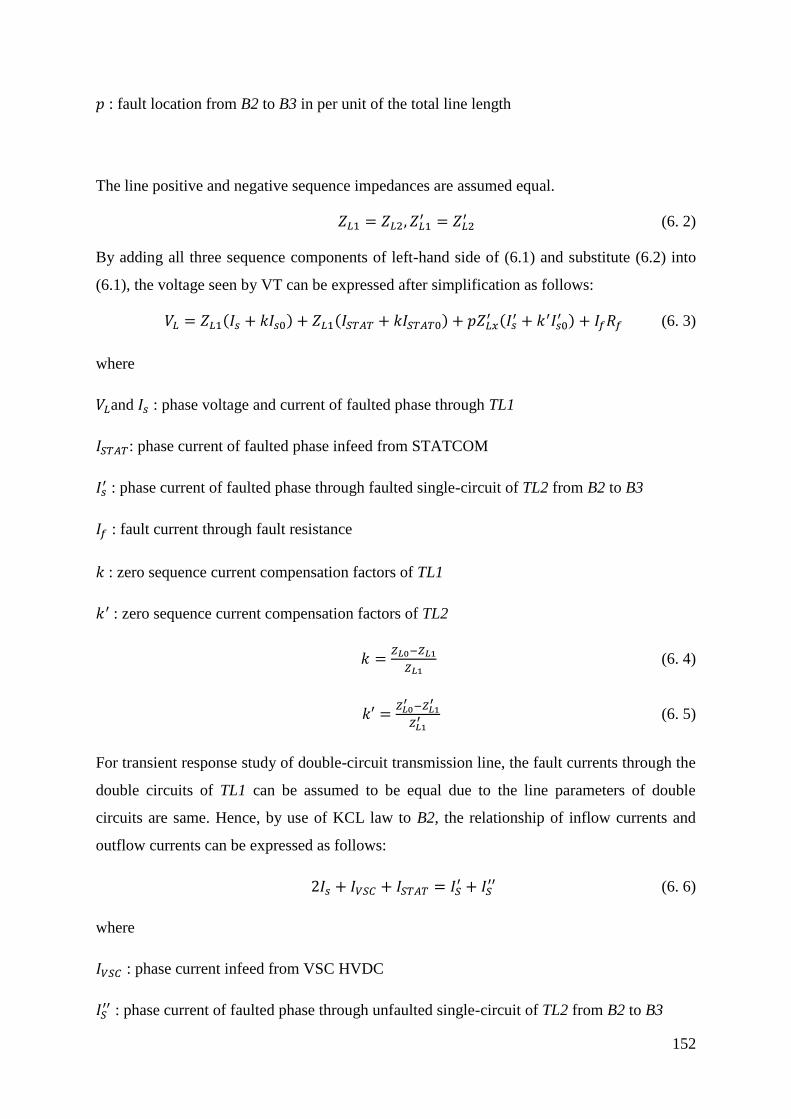
152




′ (6. 2)


(6.1), the voltage seen by VT can be expressed after simplification as follows:

𝑉𝐿 = 𝑍𝐿 (𝐼𝑠 + 𝑘𝐼𝑠0) + 𝑍𝐿 (𝐼𝑆𝑇𝐴𝑇 + 𝑘𝐼𝑆𝑇𝐴𝑇0) + 𝑝𝑍𝐿𝑥′ (𝐼𝑠

′ + 𝑘′𝐼𝑠0′ ) + 𝐼𝑓𝑅𝑓 (6. 3)

where


𝐼𝑆𝑇𝐴𝑇: phase current of faulted phase infeed from STATCOM






𝑍𝐿1 (6. 4)

𝑘′ =𝑍𝐿0

′ −𝑍𝐿1′

𝑍𝐿1′ (6. 5)





2𝐼𝑠 + 𝐼𝑉𝑆𝐶 + 𝐼𝑆𝑇𝐴𝑇 = 𝐼𝑆′ + 𝐼𝑆

′′ (6. 6)

where



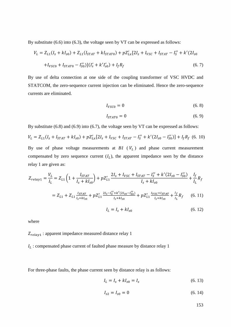
153

By substitute (6.6) into (6.3), the voltage seen by VT can be expressed as follows:

𝑉𝐿 = 𝑍𝐿 (𝐼𝑠 + 𝑘𝐼𝑠0) + 𝑍𝐿 (𝐼𝑆𝑇𝐴𝑇 + 𝑘𝐼𝑆𝑇𝐴𝑇0) + 𝑝𝑍𝐿𝑥′ [2𝐼𝑠 + 𝐼𝑉𝑆𝐶 + 𝐼𝑆𝑇𝐴𝑇 − 𝐼𝑆

′′ + 𝑘′(2𝐼𝑠0

+𝐼𝑉𝑆𝐶0 + 𝐼𝑆𝑇𝐴𝑇0 − 𝐼𝑆0′′ )](𝐼𝑠

′ + 𝑘′𝐼𝑠0′ ) + 𝐼𝑓𝑅𝑓 (6. 7)

By use of delta connection at one side of the coupling transformer of VSC HVDC and

STATCOM, the zero-sequence current injection can be eliminated. Hence the zero-sequence

currents are eliminated.

𝐼𝑉𝑆𝐶0 = 0 (6. 8)

𝐼𝑆𝑇𝐴𝑇0 = 0 (6. 9)

By substitute (6.8) and (6.9) into (6.7), the voltage seen by VT can be expressed as follows:

𝑉𝐿 = 𝑍𝐿 (𝐼𝑠 + 𝐼𝑆𝑇𝐴𝑇 + 𝑘𝐼𝑠0) + 𝑝𝑍𝐿𝑥′ [2𝐼𝑠 + 𝐼𝑉𝑆𝐶 + 𝐼𝑆𝑇𝐴𝑇 − 𝐼𝑆

′′ + 𝑘′(2𝐼𝑠0 − 𝐼𝑆0′′ )] + 𝐼𝑓𝑅𝑓 (6. 10)


compensated by zero sequence current (𝐼𝐿), the apparent impedance seen by the distance

relay 1 are given as:


𝐼𝐿= 𝑍𝐿 (1 +


𝐼𝑠 + 𝑘𝐼𝑠0) + 𝑝𝑍𝐿

′2𝐼𝑠 + 𝐼𝑉𝑆𝐶 + 𝐼𝑆𝑇𝐴𝑇 − 𝐼𝑆

′′ + 𝑘′(2𝐼𝑠0 − 𝐼𝑆0′′ )


𝐼𝑓

𝐼𝐿𝑅𝑓


𝐼𝑠+𝑘𝐼𝑠0+ 𝑝𝑍𝐿

′ 𝐼𝑠−𝐼𝑆′′+𝑘′( 𝐼𝑠0−𝐼𝑆0

′′ )


′ 𝐼𝑉𝑆𝐶+𝐼𝑆𝑇𝐴𝑇


𝐼𝑓

𝐼𝐿𝑅𝑓 (6. 11)

𝐼𝐿 = 𝐼𝑠 + 𝑘𝐼𝑠0 (6. 12)

where

𝑍𝑟𝑒𝑙𝑎𝑦 : apparent impedance measured distance relay 1

𝐼𝐿 : compensated phase current of faulted phase measure by distance relay 1


𝐼𝐿 = 𝐼𝑠 + 𝑘𝐼𝑠0 = 𝐼𝑠 (6. 13)

𝐼𝑠 = 𝐼𝑠0 = 0 (6. 14)

154


′ = 0 (6. 15)



𝐼𝐿= 𝑍𝐿 (1 +


𝐼𝑠) + 𝑝𝑍𝐿


′′

𝐼𝑠+

𝐼𝑓

𝐼𝐿𝑅𝑓






𝐼𝑠+

𝐼𝑓

𝐼𝐿𝑅𝑓 (6. 16)

By carefully looking into (6.11) and (6.16), the impacts of VSC HVDC and VSC FACTS

connected to different buses on apparent impedance measured by distance relay against

external faults can be summarised as:


′′+𝑘′( 𝐼𝑠0−𝐼𝑆0′′ )



𝐼𝑠) of (6.11)



𝐼𝑠𝑅𝑓 ) represents the contribution of fault

resistance. These terms (the first, third and fifth) are not affected by VSC HVDC and

VSC FACTS.

2. The second and fourth terms (𝑍𝐿 𝐼𝑆𝑇𝐴𝑇



𝐼𝑠+𝑘𝐼𝑠0and 𝑍𝐿




𝐼𝑠)

of (6.11) and (6.16) indicates the impacts of VSC HVDC and VSC FACTS connected to

different buses on distance relay against external faults lead to greater apparent

impedance measurements. The under-reach effect is introduced as their impacts. Since

during external fault, the VSC HVDC and STATCOM are injecting reactive power and

current to support bus voltage, the apparent impedance is greater than no VSC HVDC or

STATCOM. For steady state, while they are absorbing reactive power and current from

busbars, the second and fourth terms could be negative. This negative value indicates

less apparent impedance, which results in overreach effect. This error in apparent

impedance measurement is related to fault location, and the current ratio of VSC

HVDC/VSC FACTS and relay. For VSC HVDC and VSC FACTS connected to different

buses, their impacts on distance protection are generally combination of their separate

impacts.

155

6.2.2 VSC HVDC and VSC FACTS Connected to Same Bus


impacts of VSC HVDC and VSC FACTS connected simultaneously to same bus on distance

protection of two-ended double-circuit transmission lines. Same topology of transmission

system is studied as presented in 6.2.1, while the STATCOM is connected to B2 the same bus

with VSC HVDC. Same parameters and settings of transmission lines, power system,

distance relays, STATCOM, and VSC HVDC are used as those studied in 6.2.1.

TL1 TL2

B1

CB1 CB2

Distance

Relay 1

Distance

Relay 2

B2 B3

VSC

HVDC

ZL

IVSC

Is

If

Rf

pZ’L

VLVR

I’s (1-p)Z’L

I’’

s

STATCOM

ISTAT

Figure 6- 2 Simplified single line diagram of a faulted network for the analysis of impact of VSC

HVDC and VSC FACTS connected to same bus.

The impacts of VSC HVDC and VSC FACTS connected to the same bus on Zone 1

protection are the same with the impacts of VSC FACTS alone that has been studied in

Chapter 5, since VSC HVDC has no significant impacts on Zone 1 protection as studied in

Chapter 4. The impacts of VSC HVDC and VSC FACTS connected to the same bus on Zone

2 protection are studied since they both have significant impacts on Zone 2 protection.

The apparent impedance of VSC HVDC and VSC FACTS connected transmission line

measured by distance relays are derived for SLG faults and three-phase faults to investigate

their impacts.


𝑉𝐿𝑥 = 𝑍𝐿𝑥𝐼𝑠𝑥 + 𝑝𝑍𝐿𝑥′ 𝐼𝑠𝑥

′ + 𝐼𝑓𝑥𝑅𝑓 (6. 17)


156

𝑉𝐿𝑥 : sequence phase voltages seen by VT at B1

𝐼𝑠𝑥 : sequence phase currents seen by CT at B1




𝑍𝐿𝑥and 𝑍𝐿𝑥′ : sequence components of the line impedance of TL1 and TL2




′ (6. 18)


(6.17), the voltage seen by VT can be expressed after simplification as follows:

𝑉𝐿 = 𝑍𝐿 (𝐼𝑠 + 𝑘𝐼𝑠0) + 𝑝𝑍𝐿𝑥′ (𝐼𝑠

′ + 𝑘′𝐼𝑠0′ ) + 𝐼𝑓𝑅𝑓 (6. 19)

where







𝑍𝐿1 (6. 20)

𝑘′ =𝑍𝐿0

′ −𝑍𝐿1′

𝑍𝐿1′ (6. 21)



157



2𝐼𝑠 + 𝐼𝑉𝑆𝐶 + 𝐼𝑆𝑇𝐴𝑇 = 𝐼𝑆′ + 𝐼𝑆

′′ (6. 22)

where


𝐼𝑆𝑇𝐴𝑇: phase current of faulted phase infeed from STATCOM


By substitute (6.22) into (6.19), the voltage seen by VT can be expressed as follows:

𝑉𝐿 = 𝑍𝐿 (𝐼𝑠 + 𝑘𝐼𝑠0)

+𝑝𝑍𝐿𝑥′ [2𝐼𝑠 + 𝐼𝑉𝑆𝐶 + 𝐼𝑆𝑇𝐴𝑇 − 𝐼𝑆

′′ + 𝑘′(2𝐼𝑠0 + 𝐼𝑉𝑆𝐶0 + 𝐼𝑆𝑇𝐴𝑇0 − 𝐼𝑆0′′ )](𝐼𝑠

′ + 𝑘′𝐼𝑠0′ ) + 𝐼𝑓𝑅𝑓(6. 23)

By use of delta connection at one side of the coupling transformer of VSC HVDC and

STATCOM, the zero-sequence current injection can be eliminated. Hence the zero-sequence

currents are eliminated.

𝐼𝑉𝑆𝐶0 = 0 (6. 24)

𝐼𝑆𝑇𝐴𝑇0 = 0 (6. 25)

By substitute (6.24) and (6.25) into (6.23), the voltage seen by VT can be expressed as

follows:

𝑉𝐿 = 𝑍𝐿 (𝐼𝑠 + 𝑘𝐼𝑠0) + 𝑝𝑍𝐿𝑥′ [2𝐼𝑠 + 𝐼𝑉𝑆𝐶 + 𝐼𝑆𝑇𝐴𝑇 − 𝐼𝑆

′′ + 𝑘′(2𝐼𝑠0 − 𝐼𝑆0′′ )] + 𝐼𝑓𝑅𝑓 (6. 26)


compensated by zero sequence current (𝐼𝐿), the apparent impedance seen by Distance relay 1

is given as:




′′ + 𝑘′(2𝐼𝑠0 − 𝐼𝑆0′′ )


𝐼𝑓

𝐼𝐿𝑅𝑓


′′+𝑘′( 𝐼𝑠0−𝐼𝑆0′′ )




𝐼𝑓

𝐼𝐿𝑅𝑓 (6. 27)

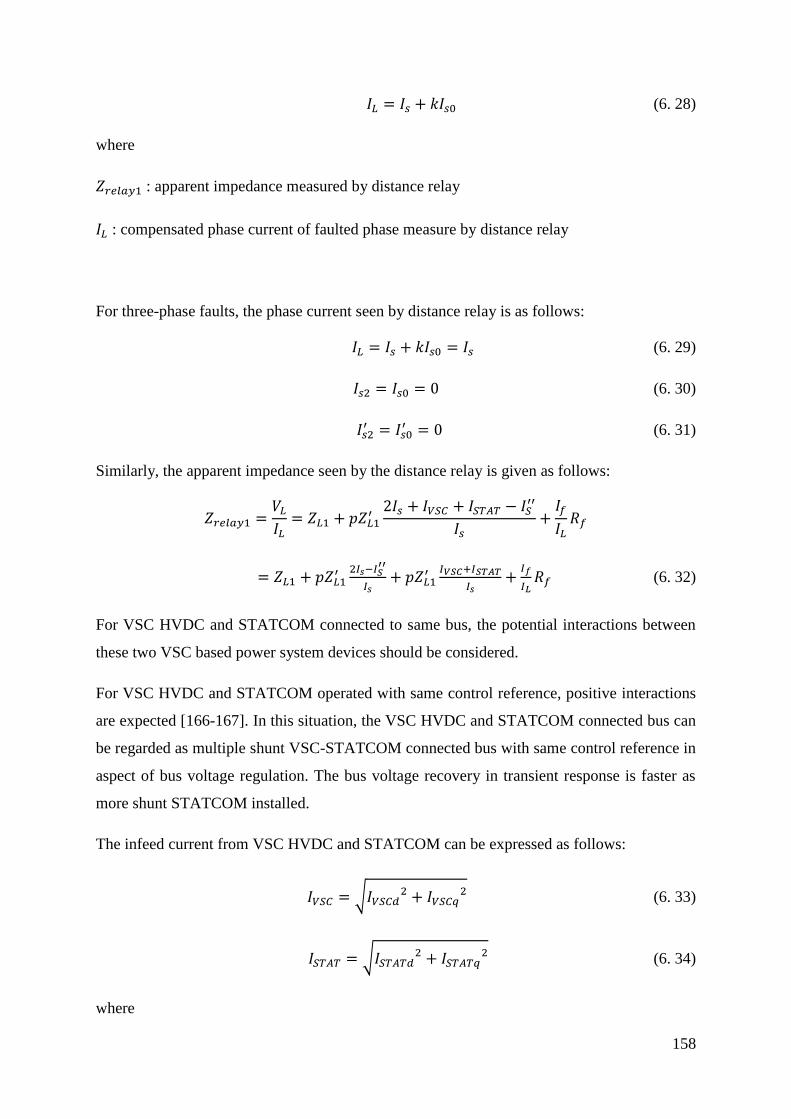
158

𝐼𝐿 = 𝐼𝑠 + 𝑘𝐼𝑠0 (6. 28)

where

𝑍𝑟𝑒𝑙𝑎𝑦 : apparent impedance measured by distance relay

𝐼𝐿 : compensated phase current of faulted phase measure by distance relay


𝐼𝐿 = 𝐼𝑠 + 𝑘𝐼𝑠0 = 𝐼𝑠 (6. 29)

𝐼𝑠 = 𝐼𝑠0 = 0 (6. 30)


′ = 0 (6. 31)





′′

𝐼𝑠+

𝐼𝑓

𝐼𝐿𝑅𝑓


′′



𝐼𝑠+

𝐼𝑓

𝐼𝐿𝑅𝑓 (6. 32)

For VSC HVDC and STATCOM connected to same bus, the potential interactions between

these two VSC based power system devices should be considered.

For VSC HVDC and STATCOM operated with same control reference, positive interactions

are expected [166-167]. In this situation, the VSC HVDC and STATCOM connected bus can

be regarded as multiple shunt VSC-STATCOM connected bus with same control reference in

aspect of bus voltage regulation. The bus voltage recovery in transient response is faster as

more shunt STATCOM installed.

The infeed current from VSC HVDC and STATCOM can be expressed as follows:

𝐼𝑉𝑆𝐶 = √𝐼𝑉𝑆𝐶𝑑 + 𝐼𝑉𝑆𝐶𝑞

(6. 33)

𝐼𝑆𝑇𝐴𝑇 = √𝐼𝑆𝑇𝐴𝑇𝑑 + 𝐼𝑆𝑇𝐴𝑇𝑞

(6. 34)

where

159

𝐼𝑉𝑆𝐶𝑑 and 𝐼𝑉𝑆𝐶𝑞: phase currents infeed from VSC HVDC in dq0 frame

𝐼𝑆𝑇𝐴𝑇𝑑 and 𝐼𝑆𝑇𝐴𝑇𝑞 : phase currents infeed from STATCOM in dq0 frame

For VSC HVDC and STATCOM modelled in this study and operated with same control

reference, the power rating of VSC is normally higher than that of STATCOM in practical

situation. Then the relationship of infeed currents in q-axis from VSC HVDC and

STATCOM modelled in this study with same control reference can be expressed as follows:

𝐼𝑉𝑆𝐶𝑞 > 𝐼𝑆𝑇𝐴𝑇𝑞 (6. 35)

For STATCOM with delta connection presented in Chapter 5, the relationship of infeed

currents in d-axis from VSC and STATCOM can be expressed as follows:

𝐼𝑉𝑆𝐶𝑑 > 𝐼𝑆𝑇𝐴𝑇𝑑 ≈ 0 (6. 36)

Hence the relationship of infeed current from VSC HVDC and STATCOM can be expressed

as follows:

𝐼𝑉𝑆𝐶 = √𝐼𝑉𝑆𝐶𝑑 + 𝐼𝑉𝑆𝐶𝑞

> 𝐼𝑆𝑇𝐴𝑇 = √𝐼𝑆𝑇𝐴𝑇𝑑 + 𝐼𝑆𝑇𝐴𝑇𝑞

(6. 37)

By look into the third term of (6.27) and (6.32), the relationship of error in measured apparent

impedance due to VSC HVDC (∆𝑍𝑉𝑆𝐶) and error in measured apparent impedance due to

STATCOM (∆𝑍𝑆𝑇𝐴𝑇) can be expressed as follows:

∆𝑍𝑉𝑆𝐶 = 𝑝𝑍𝐿 ′ 𝐼𝑉𝑆𝐶

𝐼𝐿> ∆𝑍𝑆𝑇𝐴𝑇 = 𝑝𝑍𝐿


𝐼𝐿 (6. 38)

For VSC HVDC and STATCOM operated with different control reference, negative

interactions are expected [166-167]. In this situation, the bus voltage recovery in transient

response is slower.

By carefully looking into (6.27) and (6.32), the impacts of VSC HVDC and VSC FACTS

connected to same bus on apparent impedance measured by distance relay against external

faults can be summarised as follows:

160


′′+𝑘′( 𝐼𝑠0−𝐼𝑆0′′ )



𝐼𝑠) of (6.27)



𝐼𝑠𝑅𝑓) represents the contribution of fault

resistance. These terms (the first, second and fourth) are not affected by compensation of

VSC HVDC and VSC FACTS connected to same bus.

2. The third terms (𝑝𝑍𝐿 ′ 𝐼𝑉𝑆𝐶+𝐼𝑆𝑇𝐴𝑇

𝐼𝑠+𝑘𝐼𝑠0 and 𝑝𝑍𝐿


𝐼𝑠) of (6.27) and (6.32) indicates that

the impacts of VSC HVDC and VSC FACTS connected to same bus on the apparent

impedance measured by distance relay against external fault lead to greater apparent

impedance measurements. The under-reach effect is introduced as their impacts. Since

during external fault, the VSC HVDC and STATCOM are injecting reactive power and

current to support bus voltage, the apparent impedance is greater than test system without

VSC HVDC and VSC FACTS. For steady state, while they are absorbing reactive power

and current from busbar, the third term could be negative. This negative value indicates

less apparent impedance, which results in overreach effect. This error in apparent

impedance measurement caused by VSC HVDC and VSC FACTS is related to the

current ratio, and fault location.

3. For VSC and STATCOM modelled in this study and operated with same control

reference, the error in measured apparent impedance due to VSC HVDC is generally

higher than error due to STATCOM.

6.2.3 VSC HVDC and Multiple VSC FACTS


impacts of VSC HVDC and multiple VSC FACTS on distance protection of two-ended

double-circuit transmission lines. Same topology of transmission system is studied as

presented in 6.2.1, while two STATCOMs are connected to B1 and B2. Same parameters and

settings of transmission lines, power system, distance relays, STATCOM, and VSC HVDC

are used as those studied in 6.2.1.

161

TL1 TL2

B1

CB1 CB2

Distance

Relay 1

Distance

Relay 2

B2 B3

VSC

HVDC

ZL

IVSC

Is

If

Rf

pZ’L

VLVR

I’s (1-p)Z’L

I’’

s

STATCOM 2

ISTAT2

STATCOM 1

ISTAT1

Figure 6- 3 Simplified single line diagram of a faulted network for the analysis of impacts of VSC

HVDC and multiple VSC FACTS.

The impacts of VSC HVDC and multiple VSC FACTS on Zone 1 protection are the same

with the impacts of VSC FACTS alone that has been studied in Chapter 5, since VSC HVDC

system has no significant impacts on Zone 1 protection as studied in Chapter 4. The impacts

of VSC HVDC and multiple VSC FACTS on Zone 2 protection against external faults are

studied since they both have significant impacts on Zone 2 protection.

The apparent impedance of VSC HVDC and multiple VSC FACTS connected transmission

line measured by Distance relay 1 is derived for SLG faults and three-phase faults to

investigate their impacts.

By use of approaches presented in 6.2.1 and 6.2.2, the voltage seen by VT at B1 against SLG

faults can be calculated as follows:




𝐼𝑠 + 𝑘𝐼𝑠0+ 𝑝𝑍𝐿

′2𝐼𝑠 − 𝐼𝑆

′′ + 𝑘′(2𝐼𝑠0 − 𝐼𝑆0′′ )

𝐼𝑠 + 𝑘𝐼𝑠0

+𝑝𝑍𝐿 ′ 𝐼𝑉𝑆𝐶+𝐼𝑆𝑇𝐴𝑇1+𝐼𝑆𝑇𝐴𝑇2


𝐼𝑓

𝐼𝐿𝑅𝑓 (6. 39)

𝐼𝐿 = 𝐼𝑠 + 𝑘𝐼𝑠0 (6. 40)

2𝐼𝑠 + 𝐼𝑉𝑆𝐶 + 𝐼𝑆𝑇𝐴𝑇 + 𝐼𝑆𝑇𝐴𝑇 = 𝐼𝑆′ + 𝐼𝑆

′′ (6. 41)

where


162

𝐼𝐿 : compensated phase current of faulted phase measure by Distance relay 1

𝐼𝑠0 : zero sequence phase currents seen by CT at B1

𝐼𝑆𝑇𝐴𝑇 and 𝐼𝑆𝑇𝐴𝑇 : phase current of faulted phase infeed from STATCOM 1 and STATCOM 2

𝐼𝑉𝑆𝐶 : phase current of faulted phase infeed from VSC HVDC

𝐼𝑠′ and 𝐼𝑆

′′: phase currents of faulted phase through faulted and unfaulted single-circuit of TL2

from B2 to B3



𝑍𝑟𝑒𝑙𝑎𝑦 : apparent impedance measured by Distance relay 1

𝑍𝐿 and 𝑍𝐿 ′ : positive sequence components of the line impedance of TL1 and TL2





𝑍𝐿1 (6. 42)

𝑘′ =𝑍𝐿0

′ −𝑍𝐿1′

𝑍𝐿1′ (6. 43)

Similarly, the apparent impedance seen by the Distance relay 1 against three-phase faults can

be calculated as follows:



𝐼𝑆𝑇𝐴𝑇1




′ 𝐼𝑉𝑆𝐶+𝐼𝑆𝑇𝐴𝑇1+𝐼𝑆𝑇𝐴𝑇2

𝐼𝑠+

𝐼𝑓

𝐼𝐿𝑅𝑓 (6. 44)

By carefully looking into (6.39) and (6.44), the impacts of VSC HVDC and multiple VSC

FACTS on apparent impedance measured by distance relay against external faults can be

summarised as follows:

163


′′+𝑘′( 𝐼𝑠0−𝐼𝑆0′′ )



𝐼𝑠) of (6.39)



𝐼𝐿𝑅𝑓 ) represents the contribution of fault

resistance. These terms (the first, third and fifth) are not affected by VSC HVDC and

multiple VSC FACTS.

2. The second and fourth terms ( 𝑍𝐿 𝐼𝑆𝑇𝐴𝑇1


′ 𝐼𝑉𝑆𝐶+𝐼𝑆𝑇𝐴𝑇1+𝐼𝑆𝑇𝐴𝑇2

𝐼𝑠+𝑘𝐼𝑠0and 𝑍𝐿

𝐼𝑆𝑇𝐴𝑇1

𝐼𝑠+

𝑝𝑍𝐿 ′ 𝐼𝑉𝑆𝐶+𝐼𝑆𝑇𝐴𝑇1+𝐼𝑆𝑇𝐴𝑇2

𝐼𝑠) of (6.39) and (6.44) indicate that the impacts of VSC HVDC and

multiple VSC FACTS on the apparent impedance measured by distance relay against

external faults lead to greater apparent impedance measurements. The under-reach effect

is introduced as their impacts. Since during external faults, the VSC HVDC and multiple

VSC FACTS are injecting reactive power and current to support bus voltage, the

apparent impedance is greater than test system without them. For steady state, while they

are absorbing reactive power and current from busbar, the second and fourth terms could

be negative. This negative value indicates less apparent impedance, which results in

overreach effect. This error in apparent impedance measurement caused by VSC HVDC

and multiple VSC FACTS is related to the current ratio, and fault location

3. For VSC HVDC and multiple STATCOM, their impacts on distance protection are

generally combination of separate impacts of VSC HVDC and STATCOM connected to

same bus and separate impacts of the other isolated STATCOM.


6.3.1 Test System with VSC HVDC and VSC FACTS and Protection Relay Settings



from B1 to B2. In this thesis, communications between relays are not considered. Same

transmission line parameters and equivalent voltage source parameters are used as those in

4.4 which are listed in Appendix B.1 and B.2. A VSC HVDC system is connected to B2. A

MMC delta connection STATCOM modelled in 5.2 is connected to B1or B2.

164

2 × 3-

Phase

Current

Signals;

2 × 3-Phase

Voltage Signals;

3-Ph I2

D/A

Conversion

3-Ph V2

TL1 TL2

B1 RTDS/RSCAD

3-Ph I1

3-PhV1

3-Ph V1 3-Ph V1

3-Ph I13-Ph I1

3-Ph V2

3-Ph I2 3-Ph I2

CB1 CB2



Physical Devices

B2B3

3-Ph V2

Physical Devices

Digital

Output

STATCOM1 STATCOM2 VSCHVDC

Figure 6- 4 RTDS based HIL test platform for VSC and STATCOM studies.

Figure 6- 4 shows the same arrangements of VTs, CTs and CBs for one of the

aforementioned series compensated lines between B1 and B2 as applied in Chapter 4. Same

distance protection as applied in Chapter 4 using GE MiCOM P40 Agile P443 distance

protection relays is used. Two VTs and two CTs at both ends of the transmission line provide

voltage and current measurements.

The following considerations are taken into account for the setting of the 2-ended distance

protections:





6.3.2 Dynamic Simulation Results of Test System with VSC HVDC and VSC FACTS at

Different Locations




3. SLG and three-phase to ground faults are considered.

165



“RYB-G”, or “R-G” for three-phase to ground, or SLG faults, respectively. Different

locations of STATCOM are noted as “VSC+STATB1”, “VSC+STATB2”, or

“VSC+STATB1+STATB2” for connection to B1, B2, or both B1and B2.

Table 6- 1 Simulation results of external fault

Case Fault

Location

Fault

Impedance

Fault

Type

Fault

Duration

Distance relay 1

No VSC VSC+

STATB1

VSC+

STATB2

VSC+STATB1

+STATB2 No STAT

1 105% 0.01Ω RYB-G 600ms II

105.5%

II

108.2%

II

107.6%

II

109.5%

2 105% 0.01Ω R-G 600ms II

105.9%

II

108.9%

II

108.3%

II

110.5%

3 105% 1Ω RYB-G 600ms II

106.1%

II

108.9%

II

108.1%

II

110.1%

4 105% 1Ω R-G 600ms II

106.5%

II

109.6%

II

108.8%

II

111.0%

5 135% 0.01Ω RYB-G 600ms II

136.5%

II

147.0%

II

145.3%

II

149.1%

6 135% 0.01Ω R-G 600ms × × × ×

7 135% 1Ω RYB-G 600ms × × × ×

8 135% 1Ω R-G 600ms × × × ×

Figure 6- 5 shows digital signals from RSCAD against a typical external fault Case 1 of

Table 6- 1 with no VSC HVDC or STATCOM, and the trajectory of impedance measurement

by distance relay. Figure 6- 6 shows digital signals from RSCAD against same external fault

with VSC HVDC and STATCOM connected to B1, and the corresponding trajectory of

impedance measurement. Figure 6- 7 shows digital signals from RSCAD against same

external fault with VSC HVDC and STATCOM connected to B2, and the corresponding

trajectory of impedance measurement. Figure 6- 8 shows digital signals from RSCAD against

same external fault with VSC HVDC and STATCOM connected to B1 and B2, and the

corresponding trajectory of impedance measurement.

166




(noted as ZIM vs ZRE). The trip signals (noted as TripA/TripB/TripC) are sent to

corresponding CBs, by judgement if calculated apparent impedance is within protection

zones. The CBs are turn off or turn on (noted as CBA/CBB/CBC), controlled by received trip

signals.

By comparison of the apparent impedances measured by distance relay in Table 4- 1, Table

5- 2, and Table 6- 1, the apparent impedance with VSC HVDC and STATCOM is greater

than impedance without them. The under-reach effect of distance relay is seen due to the

incorporation of VSC HVDC and STATCOM. The relationship of measured impedances of

VSC HVDC and different location of STATCOM can be expressed as follows:

𝑍𝑛𝑜𝑆𝑇𝐴𝑇 < 𝑍𝑆𝑇𝐴𝑇𝐵 < 𝑍𝑆𝑇𝐴𝑇𝐵 < 𝑍𝑉𝑆𝐶+𝑆𝑇𝐴𝑇𝐵 < 𝑍𝑉𝑆𝐶+𝑆𝑇𝐴𝑇𝐵 < 𝑍𝑉𝑆𝐶+𝑆𝑇𝐴𝑇𝐵 +𝑆𝑇𝐴𝑇 (6. 45)

where

𝑍𝑛𝑜𝑆𝑇𝐴𝑇: measured impedance with no STATCOM or VSC HVDC

𝑍𝑆𝑇𝐴𝑇𝐵 : measured impedance with STATCOM connected to B1

𝑍𝑆𝑇𝐴𝑇𝐵 : measured impedance with STATCOM connected to B2

𝑍𝑉𝑆𝐶+𝑆𝑇𝐴𝑇𝐵 : measured impedance with VSC HVDC and STATCOM connected to B1

(different buses)

𝑍𝑉𝑆𝐶+𝑆𝑇𝐴𝑇𝐵 : measured impedance with VSC HVDC and STATCOM connected to B2 (same

bus)

𝑍𝑉𝑆𝐶+𝑆𝑇𝐴𝑇𝐵 +𝑆𝑇𝐴𝑇 : measured impedance with VSC HVDC and STATCOM connected to B1

and B2

This relationship of measured impedances of VSC HVDC with different locations of

STATCOM is in line with the conclusions in 6. 2.

167

Figure 6- 5 Digital signals from RSCAD against external fault Case 1 of Table 6- 1 with no VSC

HVDC or STATCOM.


STATCOM connected to B1.

168




STATCOM connected to B1 and B2.

Figure 6- 9 shows the digital signals from RSCAD for a SLG external fault Case 2 of Table

6- 1 with VSC HVDC and STATCOM connected to B2. As voltage and current measurement

of VT and CT (noted as VA/VB/VC and IA/IB/IC) shown in Figure 6- 9, SLG fault occurred.

The three-phase trip signals (noted as TripA/TripB/TripC) are sent to corresponding CBs.

This is due to the fact that distance relay settings require relays trip all three phase for Zone 2

protection.

169

Figure 6- 9 Digital signals from RSCAD for a SLG external fault Case 2 with VSC HVDC and


Figure 6- 10 shows digital signals from RSCAD against a 1 Ω external fault Case 3 of Table

6- 1 with VSC HVDC and STATCOM at B2, and the trajectory of impedance measurement.


impedance against 1 Ω fault is greater than impedance against 0.01 Ω. These results are in

line with the conclusion in 6.2 that the error of measured impedance is positively related to

fault resistance.

Figure 6- 10 Digital signals from RSCAD for a 1 Ω external fault Case 3 with VSC HVDC and

STATCOM at B2.

Figure 6- 11 shows digital signals from RSCAD against a 135% external fault Case 7 of

Table 6- 1 with VSC HVDC and STATCOM at B2, and the trajectory of impedance

measurement by distance relay. It can be seen from Figure 6- 11 that the distance relay is not

tripped if the fault distance is too far. By comparison of the apparent impedances measured

170

by distance relay, the apparent impedance against 135% fault is greater than impedance

against 105% fault. These results are in line with the conclusions in 6.2 that the error of

measured impedance is positively related to fault distance.

Figure 6- 11 Digital signals from RSCAD for a 135% external fault Case 7 with VSC HVDC and

STATCOM at B2.

6.4 Summary

In this chapter, the mathematical representations of the apparent impedance measurement of

distance relay against external faults have been derived considering the infeed current from

VSC HVDC and shunt VSC FACTS connected simultaneously to different buses, VSC

HVDC and shunt VSC FACTS connected simultaneously to same bus, and VSC HVDC and

multiple shunt VSC FACTS. For the derived mathematical representation of the apparent

impedance measurement of distance relay with VSC HVDC and STATCOM connected to

different buses, some part (the first, third and fifth terms) is not affected by them while the

other part (the second and fourth terms) indicates that the impacts of VSC HVDC and VSC

FACTS connected to different buses on distance relay against external faults lead to greater

apparent impedance measurement. The under-reach effect is introduced as their impacts.

Since during the external fault, the VSC HVDC and STATCOM are injecting reactive power

and current to support bus voltage, the apparent impedance is greater than no VSC HVDC

and VSC FACTS. For steady state, while they are absorbing reactive power and current from

busbars, the second and fourth terms could be negative. This negative value indicates less

apparent impedance, which results in overreach effect. This error in apparent impedance

171

measurement caused by VSC HVDC and VSC FACTS is related to the current ratio, and

fault location. For VSC HVDC and VSC FACTS connected to different buses, their impacts

on distance protection are generally combination of their separate impacts.

For VSC HVDC and STATCOM connected to same bus, the potential interactions between

these two VSC based power system devices have be considered. The relationship of error in

measured apparent impedance due to VSC HVDC and error in measured apparent impedance

due to STATCOM can be expressed as follows:

∆𝑍𝑉𝑆𝐶 = 𝑝𝑍𝐿 ′

𝐼𝑉𝑆𝐶


′𝐼𝑆𝑇𝐴𝑇

𝐼𝐿

Hence for the derived mathematical representation of the apparent impedance measurement

of distance relay against external faults with VSC HVDC and STATCOM connected to same

bus, some part (the first, second and fourth terms) is not affected by them while the other part

(the third term) indicates greater apparent impedance measurements. The under-reach effect

is introduced as their impacts. The error in apparent impedance measurement caused by VSC

HVDC and VSC FACTS is related to the current ratio, and fault location. For VSC HVDC

and STATCOM modelled in this study and operated with same control reference, the error in

measured apparent impedance due to VSC HVDC is generally higher than error due to

STATCOM.

As for the derived mathematical representation of apparent impedance measurement of

distance relay against external faults with VSC HVDC and multiple STATCOM, some part

(the first, third and fifth terms) are not affected by compensation of VSC HVDC and multiple

STATCOM while the other part (second and fourth terms) indicates that the impacts of VSC

HVDC and multiple VSC FACTS on apparent impedance distance relay against external

faults lead to greater apparent impedance measurement. This error in apparent impedance

measurement caused by VSC HVDC and multiple VSC FACTS is related to the current ratio,

and fault location. For VSC HVDC and multiple STATCOM, their impacts on distance

protection are generally combination of separate impacts of VSC HVDC and STATCOM

connected to same bus and separate impacts of the other isolated STATCOM.

As shown in dynamic simulation results in RTDS/RSCAD, the apparent impedance with

VSC HVDC and STATCOM is greater than impedance without them, by comparison of the

172

apparent impedances measured by distance relay. The under-reach effect of distance relay is

seen due to the incorporation of VSC HVDC and STATCOM.

In general, to conclude the summaries of Chapter 4, Chapter 5, and Chapter 6, the combined

impacts of VSC HVDC and VSC FACTS connected at different busbars are combination of

the separate impacts of VSC HVDC and VSC FACTS. However, when VSC HVDC and

VSC FACTS are connected at same busbar, the control strategy and control reference matters.

Negative interactions between VSC HVDC and VSC FACTS and unstable oscillations would

show, if different voltage references are set. While under same control reference settings, the

relationship of measured impedances of VSC HVDC with different location of STATCOM

can be expressed as follows:

𝑍𝑛𝑜𝑆𝑇𝐴𝑇 < 𝑍𝑆𝑇𝐴𝑇𝐵 < 𝑍𝑆𝑇𝐴𝑇𝐵 < 𝑍𝑉𝑆𝐶+𝑆𝑇𝐴𝑇𝐵 < 𝑍𝑉𝑆𝐶+𝑆𝑇𝐴𝑇𝐵 < 𝑍𝑉𝑆𝐶+𝑆𝑇𝐴𝑇𝐵 +𝑆𝑇𝐴𝑇

The error of the measured impedance is positively related to fault resistance, and fault

distance.

173

CHAPTER 7 CONCLUSIONS AND FUTURE WORK

7.1 Conclusions


laid the foundation of VSC, which continues to advance the developments of HVDC

technology and FACTS. Nowadays, due to the ever increasing amount of the integrations of

renewable energy sources into power systems and the demand of long-distance bulk power

transmission with enhanced power system controllability and increased power transfer

capability, VSC converter based technology (in particular, VSC HVDC and VSC FACTS)

has been applied as a crucial solution to these big challenges. However, the high penetration

of these VSC based systems may introduce certain risks to the existing power systems in two

primary aspects: dynamic stability and protection.

This thesis has conducted comprehensive investigations on system dynamic stability and

protection due to the integration of VSC HVDC and VSC FACTS. The main conclusions of

the thesis on system dynamic stability studies of VSC HVDC based MTDC system can be


1. In this thesis, an integrated small-signal stability model for the study of interactions

between CFC and VSC has been established, which consists of multiple synchronous

generators with excitation system and PSS, multiple VSC converters, and DC network

with CFC. Modal analysis of small-signal stability model of multi-model system has

been conducted and the modal analysis results have been verified by the simulation

results from RTDS under both small and large AC/DC disturbances.

2. Based on the eigenvalue analysis and dynamic simulations, the incorporation of CFC has

been shown to affect dynamic stability of the existing MTDC/AC system especially the

adjacent VSC converters. Compared to eigenvalue results of AC/DC system without

CFC, there is no significant changes of values of synchronous generator related

conjugate pairs caused by the incorporation of CFC. This indicates that the corporation

of CFC has no significant impacts on dynamic stability of multi synchronous generators.

3. An approach of determining stable/unstable setting ranges of control parameters of CFC

has been presented and validated by simulation results in RTDS/RSCAD. The simulation

174

results have demonstrated that the control parameters of CFC could cause instability of

the system if they are not carefully-tuned.

4. Based on eigenvalue trajectory studies of CFC control gains, the variation of CFC

controller has shown to affect dynamic stability of CFC and VSC related modes. These

impacts of CFC on VSC have resulted in different damping characteristics of VSC

related states, as CFC controller changes. This effect can be severe and cause instability

to the AC/DC system, for extreme CFC operating conditions.

5. The variation of VSC controller has shown to affect dynamic stability of synchronous

generators, VSC, and CFC related modes, based on eigenvalue trajectory studies of VSC

control gains. These impacts have resulted in different damping characteristics of CFC

related states, as VSC controller changes. And this effect can be negative and cause

instability of the CFC integrated DC network, for extreme VSC operating conditions. It

has been found that the interactions between CFC and VSC could be severe and may

cause instability to the integrated MTDC/AC system. The proposed modelling approach

and methodology of analysis in this thesis has provided a useful foundation that can be

expanded for potential research of coordinated design of CFC control system and control

system of VSC to avoid possible negative interactions between them.

The main conclusions of the thesis on the impacts of VSC HVDC and VSC FACTS (in

particular, STATCOM as an example to study) on existing feeder distance protection can be


1. For test system without/with VSC HVDC, the apparent impedance of test system with

VSC is greater than impedance with no VSC HVDC integration. A RTDS-based HIL

testing platform has been established using realistic transmission data, practical distance

relays, VSC HVDC and multiple detailed STATCOM. The VSC HVDC’s impact on

feeder distance protection has been investigated, by conducting different types of

internal/external fault tests occurred at various distances. The under-reach effect of

distance relay has been found due to the incorporation of VSC. The error of measured

impedance has shown to be positively related to fault resistance, and fault distance.

2. The detailed representation of delta-connected MMC STATCOM has been modelled in

this thesis and its impact on feeder distance protection has been studied.

For test system without/with STATCOM against internal faults, the apparent

impedance of neighbouring distance relay with STATCOM is greater than impedance

175

with no STATCOM. The under-reach effect of neighbouring distance relay has been

found due to the incorporation of STATCOM. The error of the measured impedance

has shown to be positively related to fault resistance, and fault distance. For

impedance measurements of remote distance relay, there is no significant difference

of impedance measurement with/without STATCOM.

For test system without/with STATCOM against external faults, the apparent

impedance with STATCOM is greater than impedance with no STATCOM. The

under-reach effect of distance relay is seen. The error of measured impedance is

positively related to fault resistance, and fault distance.

3. For test system with VSC HVDC and STATCOM integrated simultaneously at different

locations, the apparent impedance with VSC HVDC and STATCOM is greater than

impedance without them. The under-reach effect of distance relay has been found due to

the incorporation of VSC HVDC and STATCOM. The relationship of error in the

measured apparent impedances due to VSC HVDC and that due to STATCOM can be

expressed as follows:

∆𝑍𝑉𝑆𝐶 = 𝑝𝑍𝐿 ′

𝐼𝑉𝑆𝐶


′𝐼𝑆𝑇𝐴𝑇

𝐼𝐿

And the relationship of measured impedances of VSC HVDC with different locations of

STATCOM can be expressed as follows:

𝑍𝑛𝑜𝑆𝑇𝐴𝑇 < 𝑍𝑆𝑇𝐴𝑇𝐵 < 𝑍𝑆𝑇𝐴𝑇𝐵 < 𝑍𝑉𝑆𝐶+𝑆𝑇𝐴𝑇𝐵 < 𝑍𝑉𝑆𝐶+𝑆𝑇𝐴𝑇𝐵 < 𝑍𝑉𝑆𝐶+𝑆𝑇𝐴𝑇𝐵 +𝑆𝑇𝐴𝑇

The impacts of the main contributions of this thesis on the industry and commerce can be

concluded as follows:

1. The dynamic analysis of the impacts of CFC on existing MTDC systems and the

interactions between CFC and VSC converters can be used as a viable methodology to

design and improve DC current flow controllers and their control systems so that they

can be installed into DC grid in practise.

2. The studies of the impacts of VSC HVDC and VSC FACTS on distance protection can

be applied for improvements of the existing distance protection schemes and design of

new distance protection schemes that considers the impacts of VSC systems.

176

7.2 Future Work

Built upon the achievements of this PhD work, the possible future works are suggested as

follows:

1. The dynamic characteristics of modulation technique of VSC converters can be

considered to reflect more accurate dynamic stability of VSC converters. The dynamic

characteristics of modulation algorithm of submodules of MMC can be considered and

the MMC converters can be applied as AC/DC converters for MTDC system.

2. Other control strategies of MTDC system can be considered, for instance voltage and

active power droop control, and power synchronization control. The study of small-

signal stability analysis of various control strategies can meet the needs of investigation

of system dynamic stability under different control targets.

3. The coordinated design of CFC control system and control system of VSC can be carried

out in order to avoid possible negative interactions between them.

4. Investigation of potential interactions between VSC HVDC and VSC FACTS can be

conducted in depth, and the mathematical analysis of these interactions can be performed

for coordinated controlled design of these two VSC based systems.

177

APPEDNDIX A

A.1 Generator Parameters

Table A- 1 Generator parameters

G1 G2 G3 G4

Rated MVA 900 900 900 900

𝑋𝐿 0.2 0.2 0.2 0.2

𝑅𝑠 0 0 0 0

𝑋𝑑 1.8 1.8 1.8 1.8

𝑋𝑑′ 0.3 0.3 0.3 0.3

𝑋𝑑′′ 0.25 0.25 0.25 0.25

𝑇𝑑𝑜′ 8 8 8 8

𝑇𝑑𝑜′′ 0.03 0.03 0.03 0.03

𝑋𝑞 1.7 1.7 1.7 1.7

𝑋𝑞′ 0.55 0.55 0.55 0.55

𝑋𝑞′′ 0.25 0.25 0.25 0.25

𝑇𝑞𝑜′ 0.4 0.4 0.4 0.4

𝑇𝑞𝑜′′ 0.05 0.05 0.05 0.05

𝐻 6.5 6.5 6.175 6.175

A.2 Excitation System Parameters

Table A- 2 Excitation system parameters

G1 G2 G3 G4

𝐾𝐴 200 200 200 200

𝑇𝐴 0.05 0.05 0.05 0.05

A.3 PSS Parameters

Table A- 3 PSS parameters

G1 G3

𝐾𝑝𝑠𝑠 10 10

𝑇𝑤 10 10

𝑇𝑎 0.05 0.05

𝑇𝑏 0.02 0.02

𝑇𝑐 0.08 0.08

178

𝑇𝑑 0.015 0.015

A.4 Transmission Line Parameters

Table A- 4 Transmission line parameters

End 1 bus index End 2 bus index Resistance

(p.u.)

Reactance

(p.u.)

Line charging

(p.u.)

1 5 0 0.0167 0

2 6 0 0.0167 0

3 11 0 0.0167 0

4 10 0 0.0167 0

5 6 0.0025 0.025 0.0437

10 11 0.0025 0.025 0.0437

6 7 0.001 0.01 0.0175

9 10 0.001 0.01 0.0175

7 8 0.0022 0.22 0.385

8 9 0.0022 0.22 0.385

A.5 Generation Data

Table A- 5 Generation data

Active power

(MW)

Reactive power

(Mvar)

G1 700 185

G2 700 235

G3 700 176

G4 700 202

A.6 Load Data

Table A- 6 Load data

Bus index Active power

(MW)

Reactive power

(Mvar)

Reactive compensation

(Mvar)

7 967 100 200

9 1767 100 350

179

A.7 VSC Parameters

Table A- 7 VSC parameters

VSC1 VSC2 VSC3

𝑅𝑐(Ω) 0.01 0.01 0.01

𝐿𝑐(𝑚𝐻) 7.18 7.18 7.18

𝐶𝑑𝑐( 𝑚𝐹) 5 5 5

A.8 DC Network Parameters

Table A- 8 DC network parameters

End 1 VSC index End 2 VSC index Resistance

(Ω)

Reactance

(H)

1 2 1 0.07

1 3 1 0.09

2 3 1 0.1

A.9 CFC Parameters

Table A- 9 CFC parameters

CFC

𝐶𝑐𝑓𝑐(𝑚𝐹) 1

𝑑𝑎 0.5

𝑑𝑐 0.5

𝑑𝑎 0.5

𝑑𝑎 0.5

180

APPENDIX B

B.1 Transmission Line Parameters

Table B- 1 Transmission line parameters

TL1 TL2

Length (km) 25.4 26.7

𝑍 (Ω/km) 0.32∠84.8° 0.31∠85.4°

𝑍0 (Ω/km) 0.85∠80.7° Z0=0.84∠80.3°

B.2 Equivalent Voltage Sources and Internal Impedance Parameters

Table B- 2 Equivalent voltage sources and internal impedance parameters

Voltage Source

1

Voltage

Source 2

Voltage level (kV) 400 400

𝑍 (Ω) 1.37∠86.5° 1.37∠86.5°

𝑍0 (Ω) 3.82∠86.5° 3.82∠86.5°

181

LIST OF PUBLICATIONS & OUTCOMES

Papers published

1. Rui Guan, Ying Xue, and Xiao-Ping Zhang, "Advanced RTDS-based Studies of the

Impact of STATCOM on Feeder Distance Protection," 14th International Conference on

Development in Power System Protection 2018 (DPSP), Belfast, 2018, pp. 1-6.

2. Ying Xue, Dechao Kong, Rui Guan, Can Li, Andrew Taylor, Ray Zhang, Xiao-Ping

Zhang, Dilan Jayaweera, "System performance studies in RTDS for a complex power

network with multiple FACTS devices," 13th IET International Conference on AC and

DC Power Transmission (ACDC 2017), Manchester, 2017, pp. 1-6.

3. Can Li, Dechao Kong, Ying Xue, Rui Guan, Andrew Taylor, Ray Zhang, Xiao-Ping

Zhang, Dilan Jayaweera, "Enhancement of power system small-signal stability by

coordinated damping control of multiple FACTS devices," 13th IET International

Conference on AC and DC Power Transmission (ACDC 2017), Manchester, 2017, pp. 1-

6.

Papers under review/preparation

4. Rui Guan, Na Deng, Ying Xue and Xiao-Ping Zhang, "Small-Signal Stability Analysis of

the Interactions between Voltage Sourced Converters and DC Current Flow Controllers,"

IEEE Access, 2018. (submitted)

5. Rui Guan, Ying Xue, and Xiao-Ping Zhang, “Impact of STATCOM on Distance

Protection for VSC and LCC HVDC Systems Connected Transmission Lines," IEEE

Power and Energy Technology Systems Journal, 2018. (under preparation)

Contribution to report:

6. “A New Independent Methodology for Protection & Control Coordination Studies Using

Real Time Digital Simulation (RTDS),” Project Report for National Grid, Mar. 2017.

182

REFERENCES

[1] S. Cole and R. Belmans, "Transmission of bulk power," IEEE Industrial Electronics Magazine,

vol. 3, no. 3, pp. 19-24, Sept. 2009.

[2] N. Flourentzou, V. G. Agelidis and G. D. Demetriades, "VSC-Based HVDC Power Transmission

Systems: An Overview," IEEE Transactions on Power Electronics, vol. 24, no. 3, pp. 592-602,

March 2009.

[3] M. P. Bahrman and B. K. Johnson, "The ABCs of HVDC transmission technologies," IEEE

Power and Energy Magazine, vol. 5, no. 2, pp. 32-44, April 2007.

[4] B. Gemmell, J. Dorn, D. Retzmann and D. Soerangr, "Prospects of multilevel VSC technologies

for power transmission," 2008 IEEE/PES Transmission and Distribution Conference and

Exposition, Chicago, IL, 2008, pp. 1-16.

[5] Global Energy Interconnection Development and Cooperation Organization, "Two replacements

of strategic vision of GEIDCO," [Online]. Available:

http://www.geidco.org/html/qqnycoen/col2015100766/column_2015100766_1.html. Accessed

on: Feb.12,2018

[6] P. Kundur, Power System Stability and Control. New York: McGraw Hill, 1994.

[7] T. Nakajima and S. Irokawa, "A control system for HVDC transmission by voltage sourced

converters," 1999 IEEE Power Engineering Society Summer Meeting. Conference Proceedings

(Cat. No.99CH36364), Edmonton, Alta., 1999, pp. 1113-1119 vol.2.

[8] S. Lefebvre, W. K. Wong, J. Reeve, J. M. Gagnon and B. K. Johnson, "Experience with

modeling MTDC systems in transient stability programs," IEEE Transactions on Power

Delivery, vol. 6, no. 1, pp. 405-413, Jan 1991.

[9] F. Schettler, H. Huang and N. Christl, "HVDC transmission systems using voltage sourced

converters design and applications," 2000 Power Engineering Society Summer Meeting (Cat.

No.00CH37134), Seattle, WA, 2000, pp. 715-720 vol. 2.

[10] G. P. Adam, K. H. Ahmed, S. J. Finney, K. Bell and B. W. Williams, "New Breed of Network

Fault-Tolerant Voltage-Source-Converter HVDC Transmission System," IEEE Transactions on

Power Systems, vol. 28, no. 1, pp. 335-346, Feb. 2013.

[11] G. Pinares and M. Bongiorno, "Modeling and Analysis of VSC-Based HVDC Systems for DC

Network Stability Studies," IEEE Transactions on Power Delivery, vol. 31, no. 2, pp. 848-856,

April 2016.

[12] C. Osauskas and A. Wood, "Small-signal dynamic modeling of HVDC systems," IEEE

Transactions on Power Delivery, vol. 18, no. 1, pp. 220-225, Jan 2003.

[13] Z. Chao, Z. Xiaoxin and L. Ruomei, "Dynamic Modeling and Transient Simulation for VSC

based HVDC in Multi-Machine System," 2006 International Conference on Power System

Technology, Chongqing, 2006, pp. 1-7.

[14] H. Liu and J. Sun, "Impedance-based stability analysis of VSC-based HVDC systems," 2013

IEEE 14th Workshop on Control and Modeling for Power Electronics (COMPEL), Salt Lake

City, UT, 2013, pp. 1-8.

http://www.geidco.org/html/qqnycoen/col2015100766/column_2015100766_1.html

183

[15] L. Zhang, L. Harnefors and H. P. Nee, "Interconnection of Two Very Weak AC Systems by

VSC-HVDC Links Using Power-Synchronization Control," IEEE Transactions on Power

Systems, vol. 26, no. 1, pp. 344-355, Feb. 2011.

[16] L. Zhang, L. Harnefors and H. P. Nee, "Modeling and Control of VSC-HVDC Links Connected

to Island Systems," IEEE Transactions on Power Systems, vol. 26, no. 2, pp. 783-793, May 2011.

[17] Y. Huang, X. Yuan, J. Hu and P. Zhou, "Modeling of VSC Connected to Weak Grid for Stability

Analysis of DC-Link Voltage Control," IEEE Journal of Emerging and Selected Topics in Power

Electronics, vol. 3, no. 4, pp. 1193-1204, Dec. 2015.

[18] L. Zhang, L. Harnefors and H. P. Nee, "Power-Synchronization Control of Grid-Connected

Voltage-Source Converters," IEEE Transactions on Power Systems, vol. 25, no. 2, pp. 809-820,

May 2010.

[19] T. Lüth, M. M. C. Merlin, T. C. Green, F. Hassan and C. D. Barker, "High-Frequency Operation

of a DC/AC/DC System for HVDC Applications," IEEE Transactions on Power Electronics, vol.

29, no. 8, pp. 4107-4115, Aug. 2014.

[20] L. Tang and B. T. Ooi, "Locating and Isolating DC Faults in Multi-Terminal DC Systems," IEEE

Transactions on Power Delivery, vol. 22, no. 3, pp. 1877-1884, July 2007.

[21] J. Cao, W. Du, H. F. Wang and S. Q. Bu, "Minimization of Transmission Loss in Meshed

AC/DC Grids With VSC-MTDC Networks," IEEE Transactions on Power Systems, vol. 28, no.

3, pp. 3047-3055, Aug. 2013.

[22] J. Yang, J. E. Fletcher and J. O'Reilly, "Short-Circuit and Ground Fault Analyses and Location in

VSC-Based DC Network Cables," IEEE Transactions on Industrial Electronics, vol. 59, no. 10,

pp. 3827-3837, Oct. 2012.

[23] C. Meyer, M. Hoing, A. Peterson and R. W. De Doncker, "Control and Design of DC Grids for

Offshore Wind Farms," IEEE Transactions on Industry Applications, vol. 43, no. 6, pp. 1475-

1482, Nov.-dec. 2007.

[24] L. Xu, L. Yao and M. Bazargan, "DC grid management of a multi-terminal HVDC transmission

system for large offshore wind farms," 2009 International Conference on Sustainable Power

Generation and Supply, Nanjing, 2009, pp. 1-7.

[25] P. F. Ribeiro, B. K. Johnson, M. L. Crow, A. Arsoy and Y. Liu, "Energy storage systems for

advanced power applications," Proceedings of the IEEE, vol. 89, no. 12, pp. 1744-1756, Dec

2001.

[26] L. Xu and L. Yao, "DC voltage control and power dispatch of a multi-terminal HVDC system for

integrating large offshore wind farms," IET Renewable Power Generation, vol. 5, no. 3, pp. 223-

233, May 2011.

[27] C. Feltes, H. Wrede, F. W. Koch and I. Erlich, "Enhanced Fault Ride-Through Method for Wind

Farms Connected to the Grid Through VSC-Based HVDC Transmission," IEEE Transactions on

Power Systems, vol. 24, no. 3, pp. 1537-1546, Aug. 2009.

[28] L. Xu, L. Yao and C. Sasse, "Grid Integration of Large DFIG-Based Wind Farms Using VSC

Transmission," IEEE Transactions on Power Systems, vol. 22, no. 3, pp. 976-984, Aug. 2007.

184

[29] P. Bresesti, W. L. Kling, R. L. Hendriks and R. Vailati, "HVDC Connection of Offshore Wind

Farms to the Transmission System," IEEE Transactions on Energy Conversion, vol. 22, no. 1,

pp. 37-43, March 2007.

[30] D. Van Hertem, M. Ghandhari and M. Delimar, "Technical limitations towards a SuperGrid — A

European prospective," 2010 IEEE International Energy Conference, Manama, 2010, pp. 302-

309.

[31] T. K. Vrana, R. E. Torres-Olguin, B. Liu and T. M. Haileselassie, "The North Sea Super Grid - a

technical perspective," 9th IET International Conference on AC and DC Power Transmission

(ACDC 2010), London, 2010, pp. 1-5.

[32] K. Rudion, A. Orths, P. B. Eriksen and Z. A. Styczynski, "Toward a Benchmark test system for

the offshore grid in the North Sea," IEEE PES General Meeting, Minneapolis, MN, 2010, pp. 1-

8.

[33] X. Chen et al., "Integrating Wind Farm to the Grid Using Hybrid Multiterminal HVDC

Technology," IEEE Transactions on Industry Applications, vol. 47, no. 2, pp. 965-972, March-

April 2011.

[34] E. Prieto-Araujo, F. Bianchi, A. Junyent-Ferre and O. Gomis-Bellmunt, "Methodology for droop

control dynamic analysis of multiterminal VSC-HVDC grids for offshore wind farms," 2014

IEEE PES General Meeting | Conference & Exposition, National Harbor, MD, 2014, pp. 1-1.

[35] L. Xu, B. W. Williams and L. Yao, "Multi-terminal DC transmission systems for connecting

large offshore wind farms," 2008 IEEE Power and Energy Society General Meeting - Conversion

and Delivery of Electrical Energy in the 21st Century, Pittsburgh, PA, 2008, pp. 1-7.

[36] J. Yang, J. E. Fletcher and J. O'Reilly, "Multiterminal DC Wind Farm Collection Grid Internal

Fault Analysis and Protection Design," IEEE Transactions on Power Delivery, vol. 25, no. 4, pp.

2308-2318, Oct. 2010.

[37] S. M. Muyeen, R. Takahashi and J. Tamura, "Operation and Control of HVDC-Connected

Offshore Wind Farm," IEEE Transactions on Sustainable Energy, vol. 1, no. 1, pp. 30-37, April

2010.

[38] Weixing Lu and Boon-Teck Ooi, "Optimal acquisition and aggregation of offshore wind power

by multiterminal voltage-source HVDC," IEEE Transactions on Power Delivery, vol. 18, no. 1,

pp. 201-206, Jan 2003.

[39] J. Arrillaga, Liu Yonghe, C. S. Crimp and M. Villablanca, "Harmonic Reduction In Group-

Connected Generators-HVDC Convertor," ICHPS V International Conference on Harmonics in

Power Systems., 1992, pp. 202-207.

[40] C. Karawita and U. D. Annakkage, "Multi-Infeed HVDC Interaction Studies Using Small-Signal

Stability Assessment," IEEE Transactions on Power Delivery, vol. 24, no. 2, pp. 910-918, April

2009.

[41] B. R. Andersen, L. Xu and K. T. G. Wong, "Topologies for VSC transmission," Seventh

International Conference on AC-DC Power Transmission, 2001, pp. 298-304.

[42] Q. Song, W. Liu, X. Li, H. Rao, S. Xu and L. Li, "A Steady-State Analysis Method for a

Modular Multilevel Converter," IEEE Transactions on Power Electronics, vol. 28, no. 8, pp.

3702-3713, Aug. 2013.

185

[43] G. T. Son et al., "Design and Control of a Modular Multilevel HVDC Converter With Redundant

Power Modules for Noninterruptible Energy Transfer," IEEE Transactions on Power Delivery,

vol. 27, no. 3, pp. 1611-1619, July 2012.

[44] J. Peralta, H. Saad, S. Dennetiere, J. Mahseredjian and S. Nguefeu, "Detailed and averaged

models for a 401-level MMC-HVDC system," 2013 IEEE Power & Energy Society General

Meeting, Vancouver, BC, 2013, pp. 1-1.

[45] H. Saad et al., "Dynamic Averaged and Simplified Models for MMC-Based HVDC

Transmission Systems," IEEE Transactions on Power Delivery, vol. 28, no. 3, pp. 1723-1730,

July 2013.

[46] M. Saeedifard and R. Iravani, "Dynamic Performance of a Modular Multilevel Back-to-Back

HVDC System," IEEE Transactions on Power Delivery, vol. 25, no. 4, pp. 2903-2912, Oct.

2010.

[47] U. N. Gnanarathna, A. M. Gole and R. P. Jayasinghe, "Efficient Modeling of Modular Multilevel

HVDC Converters (MMC) on Electromagnetic Transient Simulation Programs," IEEE

Transactions on Power Delivery, vol. 26, no. 1, pp. 316-324, Jan. 2011.

[48] R. Marquardt, "Modular Multilevel Converter: An universal concept for HVDC-Networks and

extended DC-Bus-applications," The 2010 International Power Electronics Conference - ECCE

ASIA -, Sapporo, 2010, pp. 502-507.

[49] M. Guan and Z. Xu, "Modeling and Control of a Modular Multilevel Converter-Based HVDC

System Under Unbalanced Grid Conditions," IEEE Transactions on Power Electronics, vol. 27,

no. 12, pp. 4858-4867, Dec. 2012.

[50] K. Friedrich, "Modern HVDC PLUS application of VSC in Modular Multilevel Converter

topology," 2010 IEEE International Symposium on Industrial Electronics, Bari, 2010, pp. 3807-

3810.

[51] J. Rodriguez, S. Bernet, B. Wu, J. O. Pontt and S. Kouro, "Multilevel Voltage-Source-Converter

Topologies for Industrial Medium-Voltage Drives," IEEE Transactions on Industrial

Electronics, vol. 54, no. 6, pp. 2930-2945, Dec. 2007.

[52] Xiao-Ping Zhang, "Multiterminal voltage-sourced converter-based HVDC models for power

flow analysis," IEEE Transactions on Power Systems, vol. 19, no. 4, pp. 1877-1884, Nov. 2004.

[53] S. Allebrod, R. Hamerski and R. Marquardt, "New transformerless, scalable Modular Multilevel

Converters for HVDC-transmission," 2008 IEEE Power Electronics Specialists Conference,

Rhodes, 2008, pp. 174-179.

[54] S. Debnath, J. Qin, B. Bahrani, M. Saeedifard and P. Barbosa, "Operation, Control, and

Applications of the Modular Multilevel Converter: A Review," IEEE Transactions on Power

Electronics, vol. 30, no. 1, pp. 37-53, Jan. 2015.

[55] S. Kouro et al., "Recent Advances and Industrial Applications of Multilevel Converters," IEEE

Transactions on Industrial Electronics, vol. 57, no. 8, pp. 2553-2580, Aug. 2010.

[56] Y. Cheng, C. Qian, M. L. Crow, S. Pekarek and S. Atcitty, "A Comparison of Diode-Clamped

and Cascaded Multilevel Converters for a STATCOM With Energy Storage," IEEE Transactions

on Industrial Electronics, vol. 53, no. 5, pp. 1512-1521, Oct. 2006.

186

[57] D. Soto and T. C. Green, "A comparison of high-power converter topologies for the

implementation of FACTS controllers," IEEE Transactions on Industrial Electronics, vol. 49, no.

5, pp. 1072-1080, Oct 2002.

[58] A. M. Gole and V. K. Sood, "A static compensator model for use with electromagnetic transients

simulation programs," IEEE Transactions on Power Delivery, vol. 5, no. 3, pp. 1398-1407, Jul

1990.

[59] F. Z. Peng and Jin Wang, "A universal STATCOM with delta-connected cascade multilevel

inverter," 2004 IEEE 35th Annual Power Electronics Specialists Conference (IEEE Cat.

No.04CH37551), 2004, pp. 3529-3533 Vol.5.

[60] P. S. Sensarma, K. R. Padiyar and V. Ramanarayanan, "Analysis and performance evaluation of

a distribution STATCOM for compensating voltage fluctuations," IEEE Transactions on Power

Delivery, vol. 16, no. 2, pp. 259-264, Apr 2001.

[61] N. Mithulananthan, C. A. Canizares, J. Reeve and G. J. Rogers, "Comparison of PSS, SVC, and

STATCOM controllers for damping power system oscillations," IEEE Transactions on Power

Systems, vol. 18, no. 2, pp. 786-792, May 2003.

[62] A. Edris, "FACTS technology development: an update," IEEE Power Engineering Review, vol.

20, no. 3, pp. 4-9, Mar 2000.

[63] Q. Song and W. Liu, "Control of a Cascade STATCOM With Star Configuration Under

Unbalanced Conditions," IEEE Transactions on Power Electronics, vol. 24, no. 1, pp. 45-58, Jan.

2009.

[64] P. Rao, M. L. Crow and Z. Yang, "STATCOM control for power system voltage control

applications," IEEE Transactions on Power Delivery, vol. 15, no. 4, pp. 1311-1317, Oct 2000.

[65] C. Hochgraf and R. H. Lasseter, "Statcom controls for operation with unbalanced voltages,"

IEEE Transactions on Power Delivery, vol. 13, no. 2, pp. 538-544, Apr 1998.

[66] B. Singh, R. Saha, A. Chandra and K. Al-Haddad, "Static synchronous compensators

(STATCOM): a review," IET Power Electronics, vol. 2, no. 4, pp. 297-324, July 2009.

[67] Yiqiao Liang and C. O. Nwankpa, "A new type of STATCOM based on cascading voltage

source inverters with phase-shifted unipolar SPWM," Conference Record of 1998 IEEE Industry

Applications Conference. Thirty-Third IAS Annual Meeting (Cat. No.98CH36242), St. Louis,

MO, USA, 1998, pp. 1447-1453 vol.2.

[68] Z. Liu, B. Liu, S. Duan and Y. Kang, "A Novel DC Capacitor Voltage Balance Control Method

for Cascade Multilevel STATCOM," IEEE Transactions on Power Electronics, vol. 27, no. 1,

pp. 14-27, Jan. 2012.

[69] S. Du, J. Liu, J. Lin and Y. He, "A Novel DC Voltage Control Method for STATCOM Based on

Hybrid Multilevel H-Bridge Converter," IEEE Transactions on Power Electronics, vol. 28, no. 1,

pp. 101-111, Jan. 2013.

[70] H. Akagi, S. Inoue and T. Yoshii, "Control and Performance of a Transformerless Cascade PWM

STATCOM With Star Configuration," IEEE Transactions on Industry Applications, vol. 43, no.

4, pp. 1041-1049, July-aug. 2007.

187

[71] K. R. Padiyar and N. Prabhu, "Design and performance evaluation of subsynchronous damping

controller with STATCOM," IEEE Transactions on Power Delivery, vol. 21, no. 3, pp. 1398-

1405, July 2006.

[72] C. D. Barker and R. S. Whitehouse, "A current flow controller for use in HVDC grids," 10th IET

International Conference on AC and DC Power Transmission (ACDC 2012), Birmingham, 2012,

pp. 1-5.

[73] H. Diab, S. Tennakoon, C. Gould and M. Marei, "An investigation of power flow control

methods in multi terminal high voltage DC grids," 2015 50th International Universities Power

Engineering Conference (UPEC), Stoke on Trent, 2015, pp. 1-5.

[74] K. Rouzbehi, A. Miranian, A. Luna and P. Rodriguez, "DC Voltage Control and Power Sharing

in Multiterminal DC Grids Based on Optimal DC Power Flow and Voltage-Droop Strategy,"

IEEE Journal of Emerging and Selected Topics in Power

[75] D. Jovcic and B. T. Ooi, "Developing DC Transmission Networks Using DC Transformers,"

IEEE Transactions on Power Delivery, vol. 25, no. 4, pp. 2535-2543, Oct. 2010.

[76] R. Eriksson, "A New Control Structure for Multiterminal DC Grids to Damp Interarea

Oscillations," IEEE Transactions on Power Delivery, vol. 31, no. 3, pp. 990-998, June 2016.

[77] N. R. Chaudhuri and B. Chaudhuri, "Adaptive droop control for effective power sharing in multi-

terminal DC (MTDC) grids," 2013 IEEE Power & Energy Society General Meeting, Vancouver,

BC, 2013, pp. 1-1.

[78] L. Zhang, H. P. Nee and L. Harnefors, "Analysis of Stability Limitations of a VSC-HVDC Link

Using Power-Synchronization Control," IEEE Transactions on Power Systems, vol. 26, no. 3, pp.

1326-1337, Aug. 2011.

[79] C. D. Barker and R. Whitehouse, "Autonomous converter control in a multi-terminal HVDC

system," 9th IET International Conference on AC and DC Power Transmission (ACDC 2010),

London, 2010, pp. 1-5.

[80] J. Sun, "Autonomous Local Control and Stability Analysis of Multiterminal DC Systems," IEEE

Journal of Emerging and Selected Topics in Power Electronics, vol. 3, no. 4, pp. 1078-1089,

Dec. 2015.

[81] K. Rouzbehi, J. I. Candela, A. Luna, G. B. Gharehpetian and P. Rodriguez, "Flexible Control of

Power Flow in Multiterminal DC Grids Using DC–DC Converter," IEEE Journal of Emerging

and Selected Topics in Power Electronics, vol. 4, no. 3, pp. 1135-1144, Sept. 2016.

[82] Q. Mu, J. Liang, Y. Li and X. Zhou, "Power flow control devices in DC grids," 2012 IEEE

Power and Energy Society General Meeting, San Diego, CA, 2012, pp. 1-7.

[83] D. Jovcic, M. Hajian, H. Zhang and G. Asplund, "Power flow control in DC transmission grids

using mechanical and semiconductor based DC/DC devices," 10th IET International Conference

on AC and DC Power Transmission (ACDC 2012), Birmingham, 2012, pp. 1-6.

[84] N. Deng, P. Wang, X. P. Zhang, G. Tang and J. Cao, "A DC current flow controller for meshed

modular multilevel converter multiterminal HVDC grids," CSEE Journal of Power and Energy

Systems, vol. 1, no. 1, pp. 43-51, March 2015.

188

[85] W. Chen, X. Zhu, L. Yao, X. Ruan, Z. Wang and Y. Cao, "An Interline DC Power-Flow

Controller (IDCPFC) for Multiterminal HVDC System," IEEE Transactions on Power Delivery,

vol. 30, no. 4, pp. 2027-2036, Aug. 2015.

[86] N. Deng, P. Wang, and X.-P. Zhang, “Small-signal Stability Analysis and Control System

Design of a Meshed Multi-terminal High-Voltage Direct Current Grid with a Current Flow

Controller”, Electric Power Components and Systems, vol. 44, no.10, 1126–1137, 2016.

[87] W. A. Lewis and L. S. Tippett, "Fundamental Basis for Distance Relaying on 3-Phase Systems,"

Transactions of the American Institute of Electrical Engineers, vol. 66, no. 1, pp. 694-709, Jan.

1947.

[88] P. J. Moore, R. K. Aggarwal, H. Jiang and A. T. Johns, "New approach to distance protection for

resistive double-phase to earth faults using adaptive techniques," IEE Proceedings - Generation,

Transmission and Distribution, vol. 141, no. 4, pp. 369-376, Jul 1994.

[89] T. S. Sidhu, R. K. Varma, P. K. Gangadharan, F. A. Albasri and G. R. Ortiz, "Performance of

distance relays on shunt-FACTS compensated transmission lines," IEEE Transactions on Power

Delivery, vol. 20, no. 3, pp. 1837-1845, July 2005.

[90] A. H. Osman and O. P. Malik, "Transmission line distance protection based on wavelet

transform," IEEE Transactions on Power Delivery, vol. 19, no. 2, pp. 515-523, April 2004.

[91] P. K. Dash, A. K. Pradhan, G. Panda and A. C. Liew, "Adaptive relay setting for flexible AC

transmission systems (FACTS)," 2000 IEEE Power Engineering Society Winter Meeting.

Conference Proceedings (Cat. No.00CH37077), Singapore, 2000, pp. 1855 vol.3-.

[92] Y. Q. Xia, K. K. Li and A. K. David, "Adaptive relay setting for stand-alone digital distance

protection," IEEE Transactions on Power Delivery, vol. 9, no. 1, pp. 480-491, Jan 1994.

[93] Alstom Grid, Network Protection & Automation Guide Protective Relays, Measurement &

Control. Alstom, 2011.

[94] Zhang Zhizhe and Chen Deshu, "An Adaptive Approach in Digital Distance Protection," IEEE

Power Engineering Review, vol. 11, no. 1, pp. 44-, January 1991.

[95] P. A. Crossley and P. G. McLaren, "Distance Protection Based on Travelling Waves," IEEE

Transactions on Power Apparatus and Systems, vol. PAS-102, no. 9, pp. 2971-2983, Sept. 1983.

[96] C. Pang and M. Kezunovic, "Fast Distance Relay Scheme for Detecting Symmetrical Fault

During Power Swing," IEEE Transactions on Power Delivery, vol. 25, no. 4, pp. 2205-2212,

Oct. 2010.

[97] K. Seethalekshmi, S. N. Singh and S. C. Srivastava, "A Classification Approach Using Support

Vector Machines to Prevent Distance Relay Maloperation Under Power Swing and Voltage

Instability," IEEE Transactions on Power Delivery, vol. 27, no. 3, pp. 1124-1133, July 2012.

[98] Z. Y. Xu et al., "A Distance Protection Relay for a 1000-kV UHV Transmission Line," IEEE

Transactions on Power Delivery, vol. 23, no. 4, pp. 1795-1804, Oct. 2008.

[99] S. Jamali, "A fast adaptive digital distance protection," 2001 Seventh International Conference

on Developments in Power System Protection (IEE), Amsterdam, 2001, pp. 149-152.

[100] M. M. Eissa and M. Masoud, "A novel digital distance relaying technique for transmission line

protection," IEEE Transactions on Power Delivery, vol. 16, no. 3, pp. 380-384, Jul 2001.

189

[101] A. G. Jongepier and L. van der Sluis, "Adaptive distance protection of a double-circuit line,"

IEEE Transactions on Power Delivery, vol. 9, no. 3, pp. 1289-1297, Jul 1994.

[102] C. Schauder and H. Mehta, “Vector analysis and control of advanced static VAr

compensators,” IEE Proc. C Gen. Trans. Distrib., vol. 140, pp. 299–306, Jul. 1993.

[103] I. Papic, P. Zunko, D. Povh, and M. Weinhold, “Basic control of unified power flow

controller,” IEEE Trans. Power Syst., vol. 12, pp. 1734–1739, Nov. 1997.

[104] T. M. Haileselassie, “Control, dynamics and operation of multi-terminal VSC-HVDC

transmission systems,” Ph.D. dissertation, Norwegian University of Science and Technology,

Trondheim, Norway, 2012.

[105] T. M. Haileselassie and K. Uhlen, “Power system security in a meshed north sea HVDC grid,”

Proc. IEEE, vol. 101, no. 4, pp. 978–990, Feb. 2013.

[106] C. Dierckxsens, K. Srivastava, M. Reza, S. Cole, J. Beerten, and R. Belmans, “A distributed

DC voltage control method for VSC MTDC systems,” Elect. Power Syst. Res., vol. 82, no. 1, pp.

54–58, Jan. 2012.

[107] K. Ou, H. Rao, Z. Cai, H. Guo, X. Lin, L. Guan, T. Maguire, B. Warkentin, and Y. Chen,

“MMC-HVDC simulation and testing based on real-time digital simulator and physical control

system,” IEEE J. Emerging and Selected Topics in Power Electron., vol. 2, no. 4, pp. 1109–

1116, Dec. 2014.

[108] J. Cao, W. Du, H. F. Wang, and S. Q. Bu, “Minimization of transmission loss in meshed

AC/DC grids with VSC-MTDC networks,” IEEE Trans. Power Syst., vol. 28, no. 3, pp. 3047–

3055, Aug. 2013.

[109] N. Yousefpoor, S. Kim, and S. Bhattacharya, “Multi-terminal DC grid control under loss of

terminal station,” IEEE Energy Conv. Cong. Exposition (ECCE), Sept. 2014, pp. 744–749.

[110] C. K. Lee, J. S. K. Leung, S. Y. R. Hui and H. S. H. Chung, "Circuit-level comparison of

STATCOM technologies," IEEE Transactions on Power Electronics, vol. 18, no. 4, pp. 1084-

1092, July 2003.

[111] D. Basic, M. Geske, J. Janning and S. Schröder, "Injection capability of delta connected

STATCOM in imbalanced situations," 2016 18th European Conference on Power Electronics

and Applications (EPE'16 ECCE Europe), Karlsruhe, 2016, pp. 1-10.

[112] A. H. Norouzi and A. M. Sharaf, "Two control schemes to enhance the dynamic performance

of the STATCOM and SSSC," IEEE Transactions on Power Delivery, vol. 20, no. 1, pp. 435-

442, Jan. 2005.

[113] M. S. El-Moursi, B. Bak-Jensen and M. H. Abdel-Rahman, "Novel STATCOM Controller for

Mitigating SSR and Damping Power System Oscillations in a Series Compensated Wind Park,"

IEEE Transactions on Power Electronics, vol. 25, no. 2, pp. 429-441, Feb. 2010.

[114] M. Hagiwara, R. Maeda and H. Akagi, "Negative-Sequence Reactive-Power Control by a

PWM STATCOM Based on a Modular Multilevel Cascade Converter (MMCC-SDBC)," IEEE

Transactions on Industry Applications, vol. 48, no. 2, pp. 720-729, March-April 2012.

[115] Z. He et al., "Reactive Power Strategy of Cascaded Delta-Connected STATCOM Under

Asymmetrical Voltage Conditions," IEEE Journal of Emerging and Selected Topics in Power

Electronics, vol. 5, no. 2, pp. 784-795, June 2017.

190

[116] C. Han et al., "STATCOM Impact Study on the Integration of a Large Wind Farm into a Weak

Loop Power System," IEEE Transactions on Energy Conversion, vol. 23, no. 1, pp. 226-233,

March 2008.

[117] B. Singh, S. S. Murthy and S. Gupta, "STATCOM-Based Voltage Regulator for Self-Excited

Induction Generator Feeding Nonlinear Loads," IEEE Transactions on Industrial Electronics,

vol. 53, no. 5, pp. 1437-1452, Oct. 2006.

[118] A. Jain, K. Joshi, A. Behal and N. Mohan, "Voltage regulation with STATCOMs: modeling,

control and results," IEEE Transactions on Power Delivery, vol. 21, no. 2, pp. 726-735, April

2006.

[119] G. Kish, R. Shi and P. Lehn, "The delta configured modular multilevel converter," 2016 IEEE

Power and Energy Society General Meeting (PESGM), Boston, MA, 2016, pp. 1-1.

[120] P. Sochor and H. Akagi, "Theoretical Comparison in Energy-Balancing Capability Between

Star- and Delta-Configured Modular Multilevel Cascade Inverters for Utility-Scale Photovoltaic

Systems," IEEE Transactions on Power Electronics, vol. 31, no. 3, pp. 1980-1992, March 2016.

[121] H. M. P. and M. T. Bina, "A Transformerless Medium-Voltage STATCOM Topology Based on

Extended Modular Multilevel Converters," IEEE Transactions on Power Electronics, vol. 26, no.

5, pp. 1534-1545, May 2011.

[122] B. Gultekin and M. Ermis, "Cascaded Multilevel Converter-Based Transmission STATCOM:

System Design Methodology and Development of a 12 kV ±12 MVAr Power Stage," IEEE

Transactions on Power Electronics, vol. 28, no. 11, pp. 4930-4950, Nov. 2013.

[123] W. Song and A. Q. Huang, "Fault-Tolerant Design and Control Strategy for Cascaded H-Bridge

Multilevel Converter-Based STATCOM," IEEE Transactions on Industrial Electronics, vol. 57,

no. 8, pp. 2700-2708, Aug. 2010.

[124] J. A. Barrena, L. Marroyo, M. Á. Rodriguez Vidal and J. R. Torrealday Apraiz, "Individual

Voltage Balancing Strategy for PWM Cascaded H-Bridge Converter-Based STATCOM," IEEE

Transactions on Industrial Electronics, vol. 55, no. 1, pp. 21-29, Jan. 2008.

[125] Yiqiang Chen, B. Mwinyiwiwa, Z. Wolanski and Boon-Teck Ooi, "Regulating and equalizing

DC capacitance voltages in multilevel STATCOM," IEEE Transactions on Power Delivery, vol.

12, no. 2, pp. 901-907, Apr 1997.



[127] R. Preece and J. V. Milanović, "Tuning of a Damping Controller for Multiterminal VSC-

HVDC Grids Using the Probabilistic Collocation Method,” IEEE Trans. Power Del., vol. 29, no.

1, pp. 318-326, Feb. 2014.

[128] R. Teixeira Pinto, P. Bauer, S. F. Rodrigues, E. J. Wiggelinkhuizen, J. Pierik and B. Ferreira,

"A Novel Distributed Direct-Voltage Control Strategy for Grid Integration of Offshore Wind

Energy Systems Through MTDC Network," IEEE Transactions on Industrial Electronics, vol.

60, no. 6, pp. 2429-2441, June 2013.

[129] J. Beerten, S. Cole and R. Belmans, "A sequential AC/DC power flow algorithm for networks

containing Multi-terminal VSC HVDC systems," IEEE PES General Meeting, Minneapolis, MN,

2010, pp. 1-7.

191

[130] S. Cole, J. Beerten and R. Belmans, "Generalized Dynamic VSC MTDC Model for Power

System Stability Studies," IEEE Transactions on Power Systems, vol. 25, no. 3, pp. 1655-1662,

Aug. 2010.

[131] J. Beerten, S. Cole and R. Belmans, "Generalized steady-state VSC MTDC model for

sequential AC/DC power flow algorithms," 2013 IEEE Power & Energy Society General

Meeting, Vancouver, BC, 2013, pp. 1-1.

[132] J. Beerten, S. D'Arco and J. A. Suul, "Identification and small-signal analysis of interaction

modes in VSC MTDC systems," 2016 IEEE Power and Energy Society General Meeting

(PESGM), Boston, MA, 2016, pp. 1-1.

[133] J. Z. Zhou, H. Ding, S. Fan, Y. Zhang and A. M. Gole, "Impact of Short-Circuit Ratio and

Phase-Locked-Loop Parameters on the Small-Signal Behavior of a VSC-HVDC Converter,"

IEEE Transactions on Power Delivery, vol. 29, no. 5, pp. 2287-2296, Oct. 2014.

[134] P. Rault, F. Colas, X. Guillaud and S. Nguefeu, "Method for small signal stability analysis of

VSC-MTDC grids," 2012 IEEE Power and Energy Society General Meeting, San Diego, CA,

2012, pp. 1-7.

[135] N. R. Chaudhuri, R. Majumder, B. Chaudhuri, J. Pan and R. Nuqui, "Modeling and stability

analysis of MTDC grids for offshore wind farms: A case study on the North Sea benchmark

system," 2011 IEEE Power and Energy Society General Meeting, San Diego, CA, 2011, pp. 1-7.

[136] H. Yuan, X. Yuan and J. Hu, "Modeling of Grid-Connected VSCs for Power System Small-

Signal Stability Analysis in DC-Link Voltage Control Timescale," IEEE Transactions on Power

Systems, vol. 32, no. 5, pp. 3981-3991, Sept. 2017.

[137] J. Beerten, S. Cole and R. Belmans, "Modeling of Multi-Terminal VSC HVDC Systems With

Distributed DC Voltage Control," IEEE Transactions on Power Systems, vol. 29, no. 1, pp. 34-

42, Jan. 2014.



[139] G. O. Kalcon, G. P. Adam, O. Anaya-Lara, S. Lo and K. Uhlen, "Small-Signal Stability

Analysis of Multi-Terminal VSC-Based DC Transmission Systems," IEEE Transactions on

Power Systems, vol. 27, no. 4, pp. 1818-1830, Nov. 2012.

[140] N. R. Chaudhuri, R. Majumder and B. Chaudhuri, "Stability analysis of VSC MTDC grids

connected to multimachine ac systems," 2012 IEEE Power and Energy Society General Meeting,

San Diego, CA, 2012, pp. 1-1.

[141] N. R. Chaudhuri, R. Majumder and B. Chaudhuri, "System frequency support through multi-

terminal DC (MTDC) grids," 2013 IEEE Power & Energy Society General Meeting, Vancouver,

BC, 2013, pp. 1-1.

[142] J. Beerten, G. B. Diaz, S. D'Arco and J. A. Suul, "Comparison of small-signal dynamics in

MMC and two-level VSC HVDC transmission schemes," 2016 IEEE International Energy

Conference (ENERGYCON), Leuven, 2016, pp. 1-6.

[143] M. Sultan, J. Reeve and R. Adapa, "Combined transient and dynamic analysis of HVDC and

FACTS systems," IEEE Transactions on Power Delivery, vol. 13, no. 4, pp. 1271-1277, Oct

1998.

192

[144] L. Wang and K. H. Wang, "Dynamic Stability Analysis of a DFIG-Based Offshore Wind Farm

Connected to a Power Grid Through an HVDC Link," IEEE Transactions on Power Systems,

vol. 26, no. 3, pp. 1501-1510, Aug. 2011.

[145] T. M. Haileselassie and K. Uhlen, "Impact of DC Line Voltage Drops on Power Flow of

MTDC Using Droop Control," IEEE Transactions on Power Systems, vol. 27, no. 3, pp. 1441-

1449, Aug. 2012.

[146] S. Liu, Z. Xu, W. Hua, G. Tang and Y. Xue, "Electromechanical Transient Modeling of

Modular Multilevel Converter Based Multi-Terminal HVDC Systems," IEEE Transactions on

Power Systems, vol. 29, no. 1, pp. 72-83, Jan. 2014.

[147] P. Kundur et al., "Definition and classification of power system stability IEEE/CIGRE joint

task force on stability terms and definitions," IEEE Transactions on Power Systems, vol. 19, no.

3, pp. 1387-1401, Aug. 2004.

[148] B. Pal and B. Chaudhuri, Robust Control in Power Systems. New York, NY, USA: Springer-

Verlag, 2005.

[149] P. W. Sauer and M. A. Pai, Power System Dynamics and Stability.Englewood Cliffs, NJ:

Prentice–Hall, 1998.

[150] J. Arrillaga, High Voltage Direct Current Transmission. London, U.K.: Inst. Electr. Eng., 1998.

[151] S. D'Arco, J. Beerten and J. A. Suul, "Classification and analysis of impact on small-signal

dynamics and stability from expansion of VSC-HVDC systems to multi-terminal HVDC

grids," 13th IET International Conference on AC and DC Power Transmission (ACDC 2017),

Manchester, 2017, pp. 1-8.

[152] Y. Huang, D. Wang, L. Shang, G. Zhu, H. Tang and Y. Li, "Modeling and Stability Analysis of

DC-Link Voltage Control in Multi-VSCs With Integrated to Weak Grid," IEEE Transactions on

Energy Conversion, vol. 32, no. 3, pp. 1127-1138, Sept. 2017.

[153] P. Rault, F. Colas, X. Guillaud and S. Nguefeu, "Method for small signal stability analysis of

VSC-MTDC grids," 2012 IEEE Power and Energy Society General Meeting, San Diego, CA,

2012, pp. 1-7.

[154] A. Salemnia, M. Khederzadeh and A. Ghorbani, "Impact of static synchronous compensator

(STATCOM) on performance of distance relay," 2009 IEEE Bucharest PowerTech, Bucharest,

2009, pp. 1-8.

[155] F. A. Albasri, T. S. Sidhu and R. K. Varma, "Performance Comparison of Distance Protection

Schemes for Shunt-FACTS Compensated Transmission Lines," IEEE Transactions on Power

Delivery, vol. 22, no. 4, pp. 2116-2125, Oct. 2007.

[156] M. Khederzadeh and A. Ghorbani, "Impact of VSC-Based Multiline FACTS Controllers on

Distance Protection of Transmission Lines," IEEE Transactions on Power Delivery, vol. 27, no.

1, pp. 32-39, Jan. 2012

[157] A. Kazemi, S. Jamali and H. Shateri, "Adaptive distance protection in presence of STATCOM

on a transmission line," IEEE PES T&D 2010, New Orleans, LA, USA, 2010, pp. 1-6.

[158] R. Dubey, S. R. Samantaray and B. K. Panigrahi, "Adaptive distance protection scheme for

shunt-FACTS compensated line connecting wind farm," IET Generation, Transmission &

Distribution, vol. 10, no. 1, pp. 247-256, 1 7 2016.

193

[159] A. R. Singh, N. R. Patne, V. S. Kale and P. Khadke, "Digital impedance pilot relaying scheme

for STATCOM compensated TL for fault phase classification with fault location," IET

Generation, Transmission & Distribution, vol. 11, no. 10, pp. 2586-2598, 7 13 2017.

[160] J. Zhang, J. Suonan, Z. Jiao, G. Song and X. Su, "A Fast Full-Line Tripping Distance

Protection Method for HVDC Transmission Line," 2012 Asia-Pacific Power and Energy

Engineering Conference, Shanghai, 2012, pp. 1-5.

[161] J. Suonan, J. Zhang, Z. Jiao, L. Yang and G. Song, "Distance Protection for HVDC

Transmission Lines Considering Frequency-Dependent Parameters," IEEE Transactions on

Power Delivery, vol. 28, no. 2, pp. 723-732, April 2013.

[162] M. Zolfaghari, R. M. Chabanlo, M. Abedi and M. Shahidehpour, "A Robust Distance

Protection Approach for Bulk AC Power System Considering the Effects of HVDC Interfaced

Offshore Wind Units," IEEE Systems Journal, vol. PP, no. 99, pp. 1-10.

[163] P. Tünnerhoff, C. Petino, M. Battiato and A. Schnettler, "Distance protection for HVDC

transmission lines based on MMC modulation strategy," 2016 Electric Power Quality and Supply

Reliability (PQ), Tallinn, 2016, pp. 283-288.

[164] L. He, C. C. Liu, A. Pitto and D. Cirio, "Distance Protection of AC Grid With HVDC-

Connected Offshore Wind Generators," IEEE Transactions on Power Delivery, vol. 29, no. 2, pp.

493-501, April 2014.

[165] C. C. Teixeira and H. Leite, "The influence of a VSC based HVDC link on distance protection

relay assessed by CAPE software," 2017 IEEE Manchester PowerTech, Manchester, 2017, pp. 1-

4.

[166] L. Shen, M. Barnes and J. V. Milanović, "Interactions between STATCOM and VSC HVDC in

dynamic GB system," 7th IET International Conference on Power Electronics, Machines and

Drives (PEMD 2014), Manchester, 2014, pp. 1-6.

[167] L. Shen, M. Barnes, J. V. Milanovic, K. R. W. Bell and M. Belivanis, "Potential interactions

between VSC HVDC and STATCOM," 2014 Power Systems Computation Conference,

Wroclaw, 2014, pp. 1-7.

[168] D. Kong, A. Taylor, Y. Xue and X. P. Zhang, "A new independent methodology for protection

and control coordination studies using real time digital simulation," 13th International

Conference on Development in Power System Protection 2016 (DPSP),

Documents

Stability control and protection of power systems with VSC