Embed Size (px)
Citation preview
INTERNATIONAL JOURNAL OF c© 2014 Institute for ScientificNUMERICAL ANALYSIS AND MODELING, SERIES B Computing and InformationVolume 5, Number 1-2, Pages 66–78
STABILITY AND NUMERICAL DISPERSION ANALYSIS OF
FINITE-DIFFERENCE METHOD FOR THE
DIFFUSIVE-VISCOUS WAVE EQUATION
HAIXIA ZHAO, JINGHUAI GAO∗, AND ZHANGXIN CHEN
Abstract. The diffusive-viscous wave equation plays an important role in seismic exploration
and it can be used to explain the frequency-dependent reflections observed both in laboratory and
field data. The numerical solution to this type of wave equation is needed in practical applicationsbecause it is difficult to obtain the analytical solution in complex media. Finite-difference method
(FDM) is the most common used in numerical modeling, yet the numerical dispersion relation and
stability condition remain to be solved for the diffusive-viscous wave equation in FDM. In thispaper, we perform an analysis for the numerical dispersion and Von Neumann stability criteria of
the diffusive-viscous wave equation for second order FD scheme. New results are compared with
the results of acoustic case. Analysis reveals that the numerical dispersion is inversely proportionalto the number of grid points per wavelength for both cases of diffusive-viscous waves and acoustic
waves, but the numerical dispersion of the diffusive-viscous waves is smaller than that of acousticwaves with the same time and spatial steps due to its more restrictive stability condition, and it
requires a smaller time step for the diffusive-viscous wave equation than acoustic case.
Key words. Stability, dispersion analysis, finite-difference method, diffusive-viscous wave equa-
tion, acoustic waves
1. Introduction
The diffusive-viscous wave equation was proposed recently in the field of oiland gas exploration. The low-frequency seismic anomalies related to hydrocarbonreservoirs have lately attracted wide attention [25, 7, 17, 8]. Even though the re-lationship between the frequency-dependent reflections and fluid saturation in areservoir can be quite complex, but there is a general connection between the char-acter of porous medium saturation and seismic response. Goloshubin and Bakulinobserved phase shifts and energy redistribution between different frequencies whencomparing cases of water-saturated and gas-saturated rocks [14, 12]. Korneev etal. observed that reflections from a fluid-saturated layer have increased amplitudeand delayed traveltime at low frequencies when compared with reflections from adry layer in both laboratory and field data [17]. Those observed results cannot beexplained using Biot theory [12, 3, 4, 5, 21, 10, 2], nor by the reflection properties ofan elastic layer [17], or the squirt flow and patchy saturation models [20]. Korneevet.al. proposed a diffusive-viscous model to explain the frequency-dependent phe-nomena in fluid-saturated porous reservoirs [17]. Therefore, the diffusive-viscoustheory is important in seismic exploration, for example, it can be used for detectingand monitoring hydrocarbon reservoirs [15], and it is also essential to simulate thepropagation of the diffusive-viscous waves in practical applications.
Seismic numerical modeling is a valuable tool for seismic interpretation and anessential part of seismic inversion algorithms. Another important application ofseismic modeling is the evaluation and design of seismic surveys [6]. There are
Received by the editors February 2, 2014 and, in revised form, March 20, 2014.
2000 Mathematics Subject Classification. 35R35, 49J40, 60G40.This research was supported by National Natural Science Foundation of China (40730424) and
National Science & Technology Major Project (2011ZX05023-005).66
STABILITY AND DISPERSION ANALYSIS 67
many approaches to seismic modeling. The finite-difference method(FDM) is themost straightforward numerical approach in seismic modeling, and it is also becom-ing increasingly more important in the seismic industry and structural modelingdue to its relative accuracy and computational efficiency [22]. Some of the mostcommon FDMs used in seismic modeling are explicit, and thus conditionally stable.Generally in seismology, explicit methods are preferred over implicit ones becausethey need less computation at each time step and have the same order of accura-cy. This has been noted for FDM [6, 11]. However, the size of the time step isbounded by a stability criterion which is an important factor affecting the accura-cy of the results. Additionally, a numerical dispersion (grid dispersion) related togrid spacing has a detrimental effect on accuracy of FD scheme. It occurs becausethe actual velocity of high-frequency waves in the grid is different from the truevelocity and it can occur even when the physical problem is not dispersive [9]. Theerror introduced by numerical dispersion is dependent on the grid spacing and thesize of the time step. There are many studies in literature regarding the numericaldispersion and stability analysis for acoustic wave propagation [1, 19]. However,the numerical dispersion analysis and stability condition is rarely seen despite itssignificance in seismic exploration for the diffusive-viscous wave propagation.
Our aims in this paper are to estimate the Von Neumann stability criteria andderive the numerical dispersion relation for the finite-difference method for thediffusive-viscous wave equation proposed by Korneev [17]. We will show thatthere are some differences of stability condition and dispersion relation betweenthe diffusive-viscous wave equation and acoustic wave equation, and the dispersionof diffusive-viscous waves is smaller than that of acoustic waves with the same timeand spatial steps because of its more restrictive stability condition, and it requiresa smaller time step for the diffusive-viscous wave equation than acoustic case.
2. The diffusive-viscous theory
In this section, we will first introduce the diffusive-viscous wave equation, thengive the propagating wavenumber and attenuation coefficient of the diffusive-viscouswaves prepared for the following section.
2.1. The diffusive-viscous wave equation. The diffusive-viscous theory is pro-posed by Korneev [17, 13], which is used to explain the relationship between thefrequency dependence of reflections and the fluid saturation in a reservoir. Thediffusive-viscous wave equation in a 1-D medium is mathematically described asfollows:
(1)∂2u
∂t2+ γ
∂u
∂t− η ∂3u
∂x2∂t− υ2 ∂
2u
∂x2= 0
for (x, t) ∈ (−∞,∞)× [0,∞), where u is the wave field; γ ≥ 0, η ≥ 0 are diffusiveand viscous attenuation parameters, respectively, which are the functions of theporosity and the permeability of reservoir rocks and the viscosity and the densityof the fluid; υ is the wave propagation velocity in a non-dispersive medium. Thesecond term in (1) characterizes a diffusional dispersive force, whereas the thirdterm describes the viscosity. t is the time and x is the space variables. Equation(1) is extended to two dimensional case (2-D) as [15]
(2)∂2u
∂t2+ γ
∂u
∂t− η(
∂3u
∂x2∂t+
∂3u
∂z2∂t)− υ2(
∂2u
∂x2+∂2u
∂z2) = 0
The definitions of the variables are the same as (1), and (x, z) ∈ (−∞,∞)×(−∞,∞)are the Cartesian coordinates.
68 H. ZHAO, J. GAO, AND Z. CHEN
2.2. The propagating wavenumber and attenuation coefficient of thediffusive-viscous wave. To derive a harmonic plane wave solution of (2), wetake a form as given below
(3) u(x, z, t) = ei(ωt−k̃xx−k̃zz)
with angular frequency ω and the wave numbers k̃x, k̃z along x and z directions,respectively. And note that k̃2
x+k̃2z =k̃2, k̃ is the complex wavenumber, and it can
be in the form as
(4) k̃ = k + iα
where, k is the propagation wavenumber, and α is the attenuation coefficient ofdiffusive-viscous waves, and i =
√−1.
Substituting (3) into (2), we get
(5) −ω2 + γ(iω) + ηk̃2(iω) + υ2k̃2 = 0
From (5), we have
(6) k̃2 =ω2 − iγωυ2 + iηω
=(υ2ω2 − γηω2)− i(ηω3 + γωυ2)
υ4 + η2ω2= K̃R + iK̃I
where, K̃R
= υ2ω2−γηω2
υ4+η2ω2 , K̃I = −ηω3+γωυ2
υ4+η2ω2 are the real and imaginary parts of k̃2.
According to (4), we can also obtain
(7) k̃2 = k2 + i2kα− α2
Then, the propagation wavenumber k and attenuation coefficient α can be obtainedby combing (6) and (7) as
(8) k = ±
√√√√K̃R +√
(K̃2R + K̃2
I )
2, α =
K̃I
2k= ± K̃I
2
√K̃R+√
(K̃2R+K̃2
I )
2
The sign of the attenuation coefficient α in (8) is determined by the attenuationproperty of diffusive-viscous waves, and both k and α not only depend on parame-ters of the medium, but also vary significantly with frequency. These two variableswill be used in the following section.
3. The Von Neumann stability criteria of diffusive-viscous wave equation
Finite-difference computations require determinations of spatial and temporalsampling criteria. As pointed out by Kelly and Marfurt [16], spatial sampling isgenerally chosen to avoid numerical dispersion in solutions. Then, the temporalsampling is chosen to avoid numerical instability. The stability analysis for FDsolutions of partial differential equations is handled using a method originally de-veloped by Von Neumann [24]. In this section, we will give the stability criteria forFD solution of diffusive-viscous wave equation following this method, and comparethe results of this equation with acoustic case.
We denote the exact solution of (2) by U(x, z, t). If we assume the grid to beuniform, let h > 0 be the spatial sampling step and let (xj , zm) = (jh,mh), j =0, 1, 2, ..., Nx,m = 0, 1, 2, ..., Nz, be the nodal points and tn = n∆t, n = 1, 2, ..., Nt,be the time points with time step of ∆t, andNx, Nz are the total numbers of samplesin x, z directions, respectively; Nt is the total number of temporal samples. The val-ues of the solution at each (xj , zm, tn) are then given by U(xj , zm, tn) = Unj,m. Andwe denote the derivatives of the solution with respect to x, z, at each (xj , zm, tn)
STABILITY AND DISPERSION ANALYSIS 69
by U′
x(xj , zm, tn) = U′
xnj,m, U
′
z(xj , zm, tn) = U′
znj,m, respectively, and similarly for
higher derivatives; for example, U′′
xx(xj , zm, tn) = U′′
xxnj,m, U
′′
zz(xj , zm, tn) = U′′
zznj,m,
etc. Then we use a central difference formula to discretize U′′
xx(x, z, t), U′′
zz(x, z, t),
U′′
tt(x, z, t) by expanding U(x, z, t) in a Taylor series at j + 1, j − 1, m + 1,m − 1,and n+ 1, n− 1,respectively, given by
(9)
U′′
xx(xj , zm, tn) ≈Unj+1,m − 2Unj,m + Unj−1,m
h2,
U′′
zz(xj , zm, tn) ≈Unj,m+1 − 2Unj,m + Unj,m−1
h2,
U′′
tt(xj , zm, tn) ≈Un+1j,m − 2Unj,m + Un−1
j,m
(∆t)2
And we use a backward difference formula to discretize U′(x, z, t), by expanding
U(x, z, t) in a Taylor series at n− 1, given by
(10) U′
t (xj , zm, tn) ≈Unj,m − U
n−1j,m
∆t
We now define a numerical approximation unj,m to the exact solution Unj,m. Usingthe discretization (9) and (10), the approximate solution unj,m associated with theequation (2) in rectangular coordinates satisfies
(11)
un+1j,m = [2− 4a− γ(∆t)− 4b]unj,m
− [1− γ(∆t)− 4a]un−1j,m − a(un−1
j+1,m + un−1j−1,m + un−1
j,m+1 + un−1j,m−1)
+ (a+ b)(unj+1,m + unj−1,m + unj,m+1 + unj,m−1)
where, a = η∆th2 , b = υ2(∆t)2
h2 .The actual error of the wavefield at (xj , zm, tn) is defined as
(12) εnj,m = Unj,m − unj,mSubstituting (12) into the FD scheme (11), we obtain
(13)
Un+1j,m − {[2− 4a− γ(∆t)− 4b]Unj,m − [1− γ(∆t)− 4a]Un−1
j,m
− a(Un−1j+1,m + Un−1
j−1,m + Un−1j,m+1 + Un−1
j,m−1)
+ (a+ b)(Unj+1,m + Unj−1,m + Unj,m+1 + Unj,m−1)}= εn+1
j,m − {[2− 4a− γ(∆t)− 4b]εnj,m − [1− γ(∆t)− 4a]εn−1j,m
− a(εn−1j+1,m + εn−1
j−1,m + εn−1j,m+1 + εn−1
j,m−1)
+ (a+ b)(εnj+1,m + εnj−1,m + εnj,m+1 + εnj,m−1)}
Note that the expression of (13) on the left side is the truncation error, and theexpression of (13) on the right side is the propagation equation for actual error. Wesay that a method is numerically stable if the actual error εnj,m is bounded as n→∞.For simplicity, we will only consider the propagation of the error and assume thetruncation error is zero. For example, in the FD scheme, this assumption impliesthe error propagates according to
(14)
εn+1j,m − {[2− 4a− γ(∆t)− 4b]εnj,m − [1− γ(∆t)− 4a]εn−1
j,m
− a(εn−1j+1,m + εn−1
j−1,m + εn−1j,m+1 + εn−1
j,m−1)
+ (a+ b)(εnj+1,m + εnj−1,m + εnj,m+1 + εnj,m−1)} = 0
70 H. ZHAO, J. GAO, AND Z. CHEN
In order to analyze the stability of (14), we will decompose the error in terms ofFourier modes or waves with certain wavelengths. This approach is known as theVon Neumann method of investigating stability [23].
An error of wave type can be written as
(15)εnj,m = εnei(k̃xxj+k̃zzm)
= εnei(jhk̃x+mhk̃z)
where εn is the amplitude of the wave at time n.We substitute (15) into (14), obtaining
(16)εn+1 = εn{2− γ(∆t)− 4(a+ b)[sin2(
k̃xh
2) + sin2(
k̃zh
2)]}
− εn−1{1− γ(∆t)− 4a[sin2(k̃xh
2) + sin2(
k̃zh
2)]}
Equation (16) has been analyzed for stability providing a sufficient condition forstability by considering the ratio of the error Fourier amplitudes as a function of
time steps [23]. That is, we consider this ratio as R = εn+1
εn = εn
εn−1 to be the ratio ofsuccessive iterations. Therefore, we can insure stability by requiring that |R| ≤ 1.
We consider the stability in terms of R by dividing equation (16) by εn−1 toobtain
(17)R2 −R{2− γ(∆t)− 4(a+ b)[sin2(
k̃xh
2) + sin2(
k̃zh
2)]}
+ {1− γ(∆t)− 4a[sin2(k̃xh
2) + sin2(
k̃zh
2)]} = 0
Denoting by
(18)A = 2− γ(∆t)− 4(a+ b)[sin2(
k̃xh
2) + sin2(
k̃zh
2)],
B = 1− γ(∆t)− 4a[sin2(k̃xh
2) + sin2(
k̃zh
2)]
Then, (17) can be rewritten as
(19) R2 −AR+B = 0
such that
(20) R =A±
√(A2 − 4B)
2And the stability condition for FD scheme is turning to solve the problem as
(21) |A±
√(A2 − 4B)
2| ≤ 1
After some complex mathematical operations, A and B in (21) have to satisfy
(22)
−2 ≤ A ≤ 2,
0 ≤ B ≤ A2
4,
B ≥ −1−A,B ≥ −1 +A
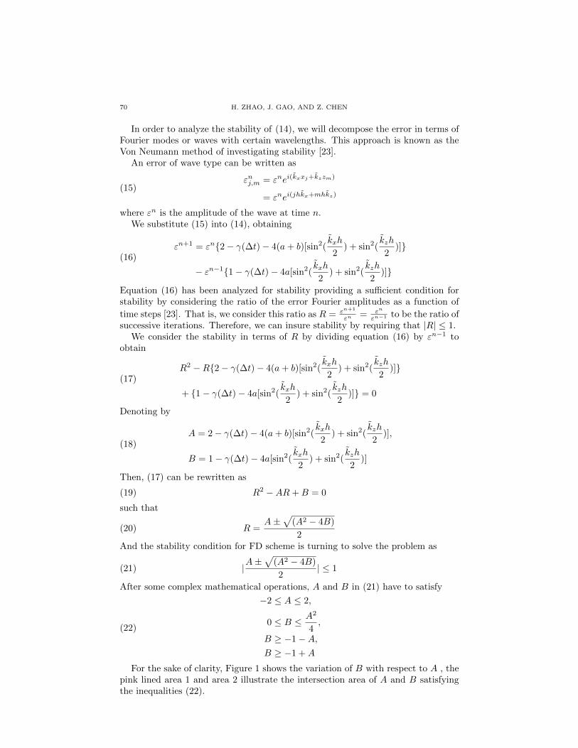
For the sake of clarity, Figure 1 shows the variation of B with respect to A , thepink lined area 1 and area 2 illustrate the intersection area of A and B satisfyingthe inequalities (22).
STABILITY AND DISPERSION ANALYSIS 71
Figure 1. Variation of B with respect to A under the conditionof the inequalities (22)
From inequality (22) and Figure 1, we can clearly see that the range of values ofA and B is
(23)−2 ≤ A ≤ 2,
0 ≤ B ≤ 1
Returning (18), we also find that
(24)2− γ(∆t)− 8(a+ b) ≤ A ≤ 2− γ(∆t),
1− γ(∆t)− 8a ≤ B ≤ 1− γ(∆t)
Inequalities (23) and (24) show that
(25)
γ ≥ 0,∆t ≥ 0,
∆t ≤√
6
4
h
υ,
∆t ≤ h2
γh2 + 8η
The inequalities (25) imply that the time step ∆t must satisfy (26) in orderto ensure the stability of second order FD scheme for the diffusive-viscous waveequation (2).
(26) 0 ≤ ∆t ≤ min(
√6
4
h
υ,
h2
γh2 + 8η)
Where, ”min” represents the minimum value of quantities.The diffusive-viscous wave equation is reduced to acoustic wave equation when
γ = η = 0. In this case, the Von Neumann stability of acoustic wave equation canbe obtained from (21) with A = 2− 4b[sin2(kxh2 ) + sin2(kzh2 ) and B = 1 [19]. Thatis
(27) ∆t ≤ 1√2
h
υ
From (26) and (27), we can clearly find that the stability criteria of diffusive-viscous wave equation for second order FD scheme is not only determined by thespatial step and velocity of the medium, but also depends on the diffusive andviscous attenuation parameter γ and η. However, it is only determined by thespatial step and velocity of the medium for acoustic case. Additionally, it requires
72 H. ZHAO, J. GAO, AND Z. CHEN
a smaller time step for diffusive-viscous wave equation than acoustic case with thesame parameters of the media and spatial steps.
4. Numerical dispersion of diffusive-viscous wave equation
In this section, we will first derive the numerical dispersion relation for thediffusive-viscous wave equation, and then we will perform the dispersion analysisnumerically for the FD scheme (11) with comparison of acoustic case.
4.1. Derivations of numerical dispersion relation. The dispersive nature ofthe waveforms can be examined by considering phase velocity as a function offrequency or, equivalently, as a function of G (the number of grid points per wave-length). The absence of dispersion would, of course, be characterized by phase ve-locity that does not vary with frequency [1]. Expression for phase velocity based onplane wave propagation of diffusive-viscous waves for the second-order FD schemeis derived in the following.
To derive the dispersion relation, the harmonic plane wave in the form of (3) isused again, and we substitute (3) into (11) and obtain
(28)
eiω(n+1)∆te−i(jhk̃ cos θ+mhk̃ sin θ)
= [2− 4a− γ(∆t)− 4b]eiωn∆te−i(jhk̃ cos θ+mhk̃ sin θ)
− [1− γ(∆t)− 4a]eiω(n−1)∆te−i(jhk̃ cos θ+mhk̃ sin θ)
− a{eiω(n−1)∆t[e−i[(j+1)hk̃ cos θ+mhk̃ sin θ] + e−i[(j−1)hk̃ cos θ+mhk̃ sin θ]
+ e−i[jhk̃ cos θ+(m+1)hk̃ sin θ] + e−i[jhk̃ cos θ+(m−1)hk̃ sin θ]]}
+ (a+ b){eiωn∆t[e−i[(j+1)hk̃ cos θ+mhk̃ sin θ] + e−i[(j−1)hk̃ cos θ+mhk̃ sin θ]
+ e−i[jhk̃ cos θ+(m+1)hk̃ sin θ] + e−i[jhk̃ cos θ+(m−1)hk̃ sin θ]]}
where θ is the angle between the direction of propagation and the x-axis.After some complex algebra operations, (28) finally becomes
(29)−4 sin2 ω∆t
2= (e−iω∆t − 1)[γ(∆t) + 4a(sin2 k̃h cos θ
2+ sin2 k̃h sin θ
2)]
− 4b(sin2 k̃h cos θ
2+ sin2 k̃h sin θ
2)
Denoting by p = υ(∆t)h and G = λ
h which is the number of grid points per wave-length, then
(30)kh
2=
2π
λ
h
2=π
G
And the normalized phase velocityCpυ is given as
(31)Cpυ
=ω
k
1
υ=ω
k
∆t
ph=ωλ
2π
∆t
ph=ω∆t
2
G
πp
Where, λ is the wavelength, and Cp = ωk is the phase velocity of the diffusive-viscous
wave equation.
Thus, the normalized phase velocityCpυ varies with G, p and ω, but the angle
frequency ω is controlled by formula (29), which implies that we cannot obtain theexplicit expression of relationship between ω and θ. From the function point of
STABILITY AND DISPERSION ANALYSIS 73
view in formula (29), the angle frequency ω is the function of θ, determined by thefollowing implicit function W (ω, θ) as
(32)W (ω, θ) = (e−iω∆t − 1)[γ(∆t) + 4a(sin2 k̃h cos θ
2+ sin2 k̃h sin θ
2)]
− 4b(sin2 k̃h cos θ
2+ sin2 k̃h sin θ
2) + 4 sin2 ω∆t
2
Substituting the expression of complex wavenumber of (4) and formula (30) into(32), one gets
(33)
W (ω, θ) = (e−iω∆t − 1){γ(∆t) + 4a[sin2(πh cos θ
G+iαh cos θ
2)
+ sin2(πh sin θ
G+iαh sin θ
2)]} − 4b[sin2(
πh cos θ
G+iαh cos θ
2)
+ sin2(πh sin θ
G+iαh sin θ
2)] + 4 sin2 ω∆t
2
where, α is the attenuation coefficient of diffusive-viscous waves, defined in (8).According to the implicit function theorem [18], there exists a function ω = f(θ)
satisfying W [f(θ), θ] = 0. However, it is impossible to obtain the exact expression ofthe function ω = f(θ) from (29), here we resort to gain the approximate relationshipbetween ω and θ using the least square method as
(34) min |W (ω, θ) |2θ=fixed value ⇒ ω ≈ f(θ)
The minimization problem (34) means that we find the values of ω when thefunction W (ω, θ) reach a minimum at fixed values of θ. So, we can obtain a seriesof values of ω when θ takes a certain range of values. From (29), (31)-(34), we can
see that the normalized phase velocityCpυ varies with θ and G, p. Therefore, from
the function point of view in formula (31), it can be rewritten as
(35) Ycp(G, θ, p) ≈ f(θ)∆t
2
G
πp
In formula (35) we have denotedCpυ by Ycp(G, θ, p).
In the case of acoustic waves, the numerical dispersion relation can be easilyobtained from (29) with γ = η = 0. That is
(36) sin2 ω∆t
2= b(sin2 kch cos θ
2+ sin2 kch sin θ
2)
In this case, kc = ωυ , α = 0. Then, the normalized phase velocity for acoustic wave
equation can be obtained from (30) and (36) as
(37)Ccpυ
=G
pπarcsin
√b[sin2(π cos θ
G ) + sin2(π sin θG )]
Where, Ccp is the phase velocity of acoustic wave.From (29) and (36), we can clearly see that the dispersion relation of diffusive-
viscous wave equation is much more complex than that of acoustic case, and itsignificantly depends on the diffusive and viscous attenuation parameters γ andη, which are determined by the properties of the media. And we can not ob-tain the explicit expression of phase velocity of diffusive-viscous wave equation butthe explicit expression of phase velocity of acoustic wave equation can be easily ob-tained. Thus, there are some differences of numerical dispersion properties betweendiffusive-viscous waves and acoustic waves for second order FDM.
74 H. ZHAO, J. GAO, AND Z. CHEN
4.2. Numerical dispersion analysis. In this section, we will present the nu-merical dispersion curves of the diffusive-viscous waves for second order FDM bycomparing those of acoustic case using the method that we presented in the pre-vious section. And we will investigate the effects that the stability parameter p,the angle θ, the number of grid points per wavelength G and the parameters of themedia have in the numerical dispersion.
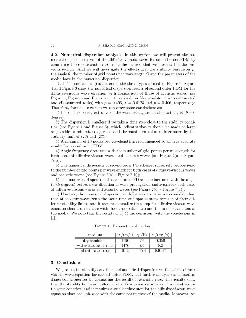
Table 1 describes the parameters of the three types of media. Figure 2, Figure4 and Figure 6 show the numerical dispersion results of second order FDM for thediffusive-viscous wave equation with comparison of those of acoustic waves (seeFigure 3, Figure 5 and Figure 7) in three medium (dry sandstone, water-saturatedand oil-saturated rocks) with p = 0.496, p = 0.6125 and p = 0.406, respectively.Therefore, from those results we can draw some conclusions as:
1) The dispersion is greatest when the wave propagates parallel to the grid (θ = 0degree);
2) The dispersion is smallest if we take a time step close to the stability condi-tion (see Figure 4 and Figure 5), which indicates that it should be made as largeas possible to minimize dispersion and the maximum value is determined by thestability limit of (26) and (27);
3) A minimum of 10 nodes per wavelength is recommended to achieve accurateresults for second order FDM;
4) Angle frequency decreases with the number of grid points per wavelength forboth cases of diffusive-viscous waves and acoustic waves (see Figure 2(a) - Figure7(a));
5) The numerical dispersion of second order FD scheme is inversely proportionalto the number of grid points per wavelength for both cases of diffusive-viscous wavesand acoustic waves (see Figure 2(b) - Figure 7(b));
6) The numerical dispersion of second order FD scheme increases with the angle(0-45 degrees) between the direction of wave propagation and x-axis for both casesof diffusive-viscous waves and acoustic waves (see Figure 2(c) - Figure 7(c));
7) However, the numerical dispersion of diffusive-viscous waves is smaller thanthat of acoustic waves with the same time and spatial steps because of their dif-ferent stability limits, and it requires a smaller time step for diffusive-viscous waveequation than acoustic case with the same spatial step and the same parameters ofthe media. We note that the results of 1)-3) are consistent with the conclusions in[1].
Table 1. Parameters of medium
medium υ /(m/s) γ /Hz η /(m2/s)
dry sandstone 1190 56 0.056water-saturated rock 1470 90 0.2
oil-saturated rock 1015 65.4 0.0147
5. Conclusions
We present the stability condition and numerical dispersion relation of the diffusive-viscous wave equation for second order FDM, and further analyze the numericaldispersion properties by comparing the results of acoustic case. The results showthat the stability limits are different for diffusive-viscous wave equation and acous-tic wave equation, and it requires a smaller time step for the diffusive-viscous waveequation than acoustic case with the same parameters of the media. Moreover, we
STABILITY AND DISPERSION ANALYSIS 75
(a) (b) (c)
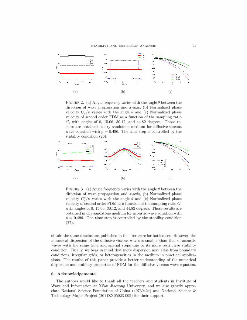
Figure 2. (a) Angle frequency varies with the angle θ between thedirection of wave propagation and x-axis, (b) Normalized phasevelocity Cp/υ varies with the angle θ and (c) Normalized phasevelocity of second order FDM as a function of the sampling ratioG, with angles of 0, 15.06, 30.12, and 44.82 degrees. Those re-sults are obtained in dry sandstone medium for diffusive-viscouswave equation with p = 0.496. The time step is controlled by thestability condition (26).
(a) (b) (c)
Figure 3. (a) Angle frequency varies with the angle θ between thedirection of wave propagation and x-axis, (b) Normalized phasevelocity Ccp/υ varies with the angle θ and (c) Normalized phasevelocity of second order FDM as a function of the sampling ratio G,with angles of 0, 15.06, 30.12, and 44.82 degrees. Those results areobtained in dry sandstone medium for acoustic wave equation withp = 0.496. The time step is controlled by the stability condition(27).
obtain the same conclusions published in the literature for both cases. However, thenumerical dispersion of the diffusive-viscous waves is smaller than that of acousticwaves with the same time and spatial steps due to its more restrictive stabilitycondition. Finally, we bear in mind that more dispersion may arise from boundaryconditions, irregular grids, or heterogeneities in the medium in practical applica-tions. The results of this paper provide a better understanding of the numericaldispersion and stability properties of FDM for the diffusive-viscous wave equation.
6. Acknowledgements
The authors would like to thank all the teachers and students in Institute ofWave and Information at Xi’an Jiaotong University, and we also greatly appre-ciate National Science Foundation of China (40730424) and National Science &Technology Major Project (2011ZX05023-005) for their support.
76 H. ZHAO, J. GAO, AND Z. CHEN
(a) (b) (c)
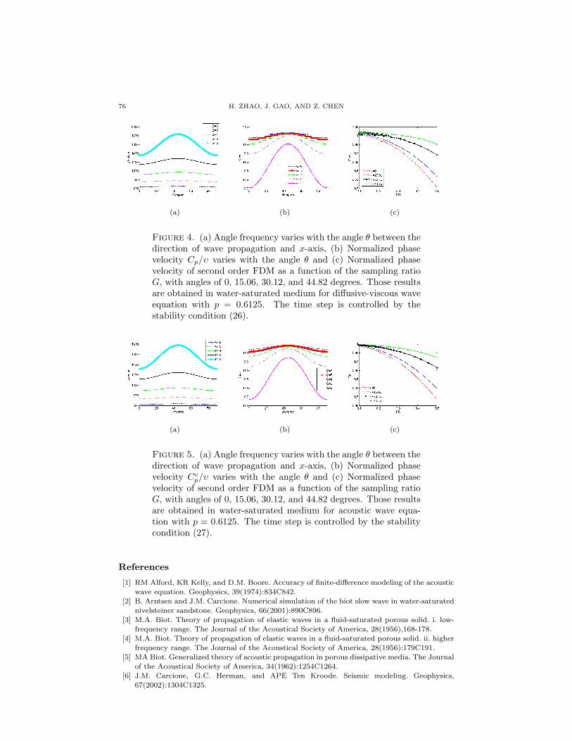
Figure 4. (a) Angle frequency varies with the angle θ between thedirection of wave propagation and x-axis, (b) Normalized phasevelocity Cp/υ varies with the angle θ and (c) Normalized phasevelocity of second order FDM as a function of the sampling ratioG, with angles of 0, 15.06, 30.12, and 44.82 degrees. Those resultsare obtained in water-saturated medium for diffusive-viscous waveequation with p = 0.6125. The time step is controlled by thestability condition (26).
(a) (b) (c)
Figure 5. (a) Angle frequency varies with the angle θ between thedirection of wave propagation and x-axis, (b) Normalized phasevelocity Ccp/υ varies with the angle θ and (c) Normalized phasevelocity of second order FDM as a function of the sampling ratioG, with angles of 0, 15.06, 30.12, and 44.82 degrees. Those resultsare obtained in water-saturated medium for acoustic wave equa-tion with p = 0.6125. The time step is controlled by the stabilitycondition (27).
References
[1] RM Alford, KR Kelly, and D.M. Boore. Accuracy of finite-difference modeling of the acousticwave equation. Geophysics, 39(1974):834C842.
[2] B. Arntsen and J.M. Carcione. Numerical simulation of the biot slow wave in water-saturatednivelsteiner sandstone. Geophysics, 66(2001):890C896.
[3] M.A. Biot. Theory of propagation of elastic waves in a fluid-saturated porous solid. i. low-frequency range. The Journal of the Acoustical Society of America, 28(1956),168-178.
[4] M.A. Biot. Theory of propagation of elastic waves in a fluid-saturated porous solid. ii. higherfrequency range. The Journal of the Acoustical Society of America, 28(1956):179C191.
[5] MA Biot. Generalized theory of acoustic propagation in porous dissipative media. The Journalof the Acoustical Society of America, 34(1962):1254C1264.
[6] J.M. Carcione, G.C. Herman, and APE Ten Kroode. Seismic modeling. Geophysics,67(2002):1304C1325.
STABILITY AND DISPERSION ANALYSIS 77
(a) (b) (c)
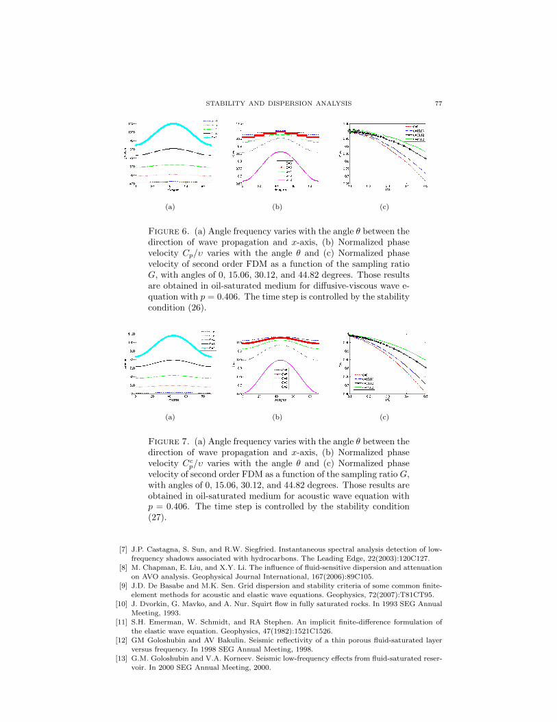
Figure 6. (a) Angle frequency varies with the angle θ between thedirection of wave propagation and x-axis, (b) Normalized phasevelocity Cp/υ varies with the angle θ and (c) Normalized phasevelocity of second order FDM as a function of the sampling ratioG, with angles of 0, 15.06, 30.12, and 44.82 degrees. Those resultsare obtained in oil-saturated medium for diffusive-viscous wave e-quation with p = 0.406. The time step is controlled by the stabilitycondition (26).
(a) (b) (c)
Figure 7. (a) Angle frequency varies with the angle θ between thedirection of wave propagation and x-axis, (b) Normalized phasevelocity Ccp/υ varies with the angle θ and (c) Normalized phasevelocity of second order FDM as a function of the sampling ratio G,with angles of 0, 15.06, 30.12, and 44.82 degrees. Those results areobtained in oil-saturated medium for acoustic wave equation withp = 0.406. The time step is controlled by the stability condition(27).
[7] J.P. Castagna, S. Sun, and R.W. Siegfried. Instantaneous spectral analysis detection of low-
frequency shadows associated with hydrocarbons. The Leading Edge, 22(2003):120C127.[8] M. Chapman, E. Liu, and X.Y. Li. The influence of fluid-sensitive dispersion and attenuation
on AVO analysis. Geophysical Journal International, 167(2006):89C105.
[9] J.D. De Basabe and M.K. Sen. Grid dispersion and stability criteria of some common finite-element methods for acoustic and elastic wave equations. Geophysics, 72(2007):T81CT95.
[10] J. Dvorkin, G. Mavko, and A. Nur. Squirt flow in fully saturated rocks. In 1993 SEG Annual
Meeting, 1993.[11] S.H. Emerman, W. Schmidt, and RA Stephen. An implicit finite-difference formulation of
the elastic wave equation. Geophysics, 47(1982):1521C1526.
[12] GM Goloshubin and AV Bakulin. Seismic reflectivity of a thin porous fluid-saturated layerversus frequency. In 1998 SEG Annual Meeting, 1998.
[13] G.M. Goloshubin and V.A. Korneev. Seismic low-frequency effects from fluid-saturated reser-voir. In 2000 SEG Annual Meeting, 2000.
78 H. ZHAO, J. GAO, AND Z. CHEN
[14] GM Goloshubin, AM Verkhovsky, and VV Kaurov. Laboratory experiments of seismic mon-
itoring. In EAGE 58th Conference and Technical Exhibition, Amsterdam, The Netherlands,
Geophysical Division, volume 2(1996):3C7.[15] Z. He, X. Xiong, and L. Bian. Numerical simulation of seismic low-frequency shadows and
its application. Applied Geophysics, 5(2008):301C306.
[16] KR Kelly. Numerical modeling of seismic wave propagation, volume 13. Soc of ExplorationGeophysicists, 1990.
[17] V.A. Korneev, G.M. Goloshubin, T.M. Daley, and D.B. Silin. Seismic low-frequency effects
in monitoring fluid-saturated reservoirs. Geophysics, 69(2004):522C532.[18] S.G. Krantz and H.R. Parks. The implicit function theorem: history, theory, and applications.
Birkh?user Boston, 2002.
[19] L.R. Lines, R. Slawinski, and R.P. Bording. A recipe for stability analysis of finite-differencewave equation computations. Geophysics, 64(1999):967C969.
[20] G. Mavko, T. Mukerji, and J. Dvorkin. Rock physics handbook: Tools for seismic interpre-tation in porous media 1998.
[21] S. Mochizuki. Attenuation in partially saturated rocks. Journal of Geophysical Research,
87(1982):8598C8604.[22] P. Moczo, J.O.A. Robertsson, and L. Eisner.The finite-difference time-domain method for
modeling of seismic wave propagation. Advances in Geophysics, 48(2007):421C516.
[23] I.R. Mufti. Large-scale three-dimensional seismic models and their interpretive signifi-cance.Geophysics, 55(1990):1166C1182.
[24] W.H. Press, B.P. Flannery, S.A. Teukolsky, and W.T. Vetterling. Numerical Recipes in FOR
TRAN 77: Volume 1, Volume 1 of Fortran Numerical Recipes: The Art of Scientific Com-puting, volume 1. Cambridge university press, 1992.
[25] M.T. Taner, F. Koehler, and RE Sheriff. Complex seismic trace analysis. Geophysic-
s,44(1979):1041C1063.
National Engineering Laboratory for Offshore Oil Exploration, Institute of Wave and Informa-
tion, School of Electronic and Information Engineering, Xi’an Jiaotong University, Xi’an 710049,
ChinaE-mail : [email protected] and [email protected]
Center for Computational Geoscience, Xi’an Jiaotong University, Xi’an 710049, China. De-partment of Chemical and Petroleum Engineering, University of Calgary,Calgary, Alberta, T2N
1N4, Canada.
E-mail : [email protected]