Embed Size (px)
Citation preview

Stability and Error Estimation for Component
Adaptive Grid Methods
Joseph Oliger and Xiaolei Zhu
The Research Institute of Advanced Computer Science is operated by Universities Space Research
Association, The American City Building, Suite 212, Columbia, MD 21044, (410) 730-2656
This work was begun with support from the Office of Naval Research under contracts N00014-89-J-185-P00006 and N00014-90-J-1344-P00005 and completed with support from the National ScienceFoundation under grant DMS-9318166 and NASA under contract NAS2-13721.
https://ntrs.nasa.gov/search.jsp?R=19950005470 2018-06-13T17:30:44+00:00Z


Abstract
Component adaptive grid (CAG) methods for solving hyperbolic partial differen-
tial equations (PDE's) are discussed in this paper. Applying recent stability results
for a class of numerical methods on uniform grids, the convergence of these methods
for linear problems on component adaptive grids is established here. Furthermore,
the computational error can be estimated on CAG's using the stability results. Using
these estimates, the error can be controlled on CAG's. Thus, the solution can be
computed efficiently on CAG's within a given error tolerance. Computational results
for time dependent linear problems in one and two space dimensions are presented.

1 Introduction
Component adaptive grid methods for solving hyperbolic PDE's were introduced in
the early 1980's. An overview of the method is given in Section 2. More details can be
found in Berger and Oliger [2], and Berger [1]. However, the grid structure used in this
paper is different from the one Berger used. As discussed in Section 2, stair step grids
like those of Chesshire and Henshaw [4] are used in our CAG methods here, instead
of rotated rectangular grids. One major component of the adaptive strategy is to
estimate the local truncation error at each grid point, then refine where the estimated
errors are larger than a given tolerance 5. The smaller _ is, the smaller the final error
is expected to be in some weighted L2 norm. However, no quantitative relationship
between these two kinds of errors had been established. Recently, new stability results
have been developed by Pelle Olsson [6] which allow us to establish such a relationship
for large classes of problems and methods. The results can be applied to various classes
of problems, e.g., those of hyperbolic, parabolic and hyperbolic-parabolic type, using
a large class of numerical methods on uniform grids. As we will see in Section 3, the
structures of component adaptive grids allow us to define the solution on piecewise
uniform grids. So the stability theories can be applied on CAG's. Convergence for
linear problems using these methods on CAG's is proved in Section 3. Also the
tolerance _ on local truncation error is estimated in term of the tolerance c on the
final error. Furthermore, the results in Section 3 will also help us estimate the final
error using simple quadrature, and serve us as guidelines on developing strategies
for CAG methods, since we have a very good understanding of the sources and the
magnitudes of various computational errors. Finally, some computional results for
time dependent problems in one and two space dimensions are given in Section 4.
2 An Overview of Component Adaptive Grids
We first introduce some notation for our discussion. Suppose the problem we wish to
solve is written as
ut = L u + f on f_× [0, T] (1)
u(0) = u0 on (2)Bu = b on 0f_×[0, T] (3)
where fl C R d is a bounded domain in physical space, L is a spatial partial differetial
operator on F/and u E/_. We assume this to be a well-posed initial-boundary value
problem which is defined in Section 3. Let F/h, Ol2h and [0, T]k be the discretizations of
_, OF/and [0, T], respectively. In Section 3, these discretizations are defined precisely
2

for our component adaptive grids. For the time being, we can consider them as
general grids.
Let Vh be a grid function defined on F/h × [0, T]k. We will discuss the use of
finite difference methods on these grids. Without loss of generality, and avoiding
complicated notation, we write our methods in explicit one-step form as
vh(t + k) = Lhvh(t) + k f_(t) on F/hx[0, T]k (4)_(0) = _o_ o_ F/_ (5)
Bhvh(t) = bh(t) on 0F/hx [0,T]k (6)
where we use subscripts to denote projections of functions onto the appropriate grids
and discretizations of operators on these grids. If Uh is the projection of the exact
solution of the above system onto F/h, then
uh(t + k) = Lh uh(t) + k fh(t) + k'rh on _h × [O,T]k (7)
where Th is the local truncation error. This notation will also be used on the piecewise
uniform grids which we will discuss next.
2.1 Composite Grids
In real applications, the physical domains often have complicated geometries. In order
to use finite difference schemes on these domains, we decompose the physical domain
and transform the parts into computational domains. However this topic is not the
focus of this paper. Here only a brief introduction is given to make our presentation
self contained. Details can be found in Chesshire and Henshaw [4], Venkata, Oliger
and Ferziger [8], and Venkata [9].
We begin by forming a base composite grid
Go= [_Jao,j (S)J
which will be characterized by a discretization parameter h0.
This is well illustrated in Figure 1 where Go consists of the component grids Go,l,
G0,2, and G0,3. G0,: is a stair step grid with grid lines parallel to the coordinate axes.
Such grids are called regular grids.
Definition 1: A regular grid is a connected stair step grid of uniformly spaced
points in each coordinate direction, and its grid lines are parallel to the coordinate
3

axesin either physical or computational space.
No coordinate transformation is neededto solvethe equation on regular grids inphysical space. The curvilinear grids G0,1 and G0,3 are defined by specifying their
boundaries and cuts. Regular girds in computational space are then mapped onto
these grids in physical space using coordinate tranformations. To reduce clutter in
Figure 1 , grids G0,1 and G0,3 are shown only in computational space. The component
grids are chosen to obtain a sufficiently accuate representation of 0R by Oglh. ho is
an estimate of the step size required to obtain a sufficiently accuate approximation of
the solution over at least some specified fraction of the domain. The difficult problem
here is to generate grids on the boundaries. The B_zier family of curves and surfaces
are used to generate boundary grids in 2-D and 3-D, respectively (see [8] and [9]).
G0, 2
G1,1
G0,3
G1,2
0,1G
1,3 G1,4
I I I I I I I I I I 1 I I I I I I I I I I I I 1 I I I I iaman"
lllllllllllllllllllllllllllllllll_ i]lllllllllllllllllllllllllllllllJl_
Figure 1: Adaptive Composite Grid Structure
2.2 Component Adaptive Grids
The component grids mentioned in Section 2.1 are specified to describe the domain
and its boundaries. Next, we will discuss the use of adaptive grids which are created

and destroyedduring the courseof the computation in order to maintain sufficientaccuracythroughout the entire domain.
During this process,wewill createL - 1 additional refinement levels of composite
grids Gl on top of the base grid Go. So the whole grid system can be written asfollows:
L-1
U a, (9)I=0
where at each level l, we have
= U c ,j. (10)j
These will have spatial discretization parameters hi = ho/m t, where m might range
from 2 to 10 depending on the problems being solved. According to Berger and Oliger
[2], m = 4 is a reasonable choice for many hyperbolic problems. We usually let L be
2, 3 or 4. As dictated by the nature of the problem and numerical algorithm, we main-
tain an appropriate relationship between the spatial and the temporal discretization
parameters, ht and kt. In particular, for problems which are essentially hyperbolic in
character, we usually use the same mesh ratio on all levels, i.e.,
= kt/ht = constant. (11)
Another very important feature for our adaptive grids is that the grids are level
nested, i.e., the region Gl is fully contained within the region Gt-1. See the shaded
refined grids Ga,x, G1,2, G1,3 and G1,4 in Figure 1. Since these grids have the same mesh
ratio, they have the space-time structure illustrated in Figure 2. We take several time
steps on the finer grid for each time step on the coarser grid.
:.,,., ======================:.:+: :.::.::i:i:|::::::::::::::,:::::::|:::::::|......•--'- ..:...:i:,:.:._t+:.:. +:.:. ::.:
::::::::::::::::::::::::::::::::::::::::::::::::::::::::::::::::::
:::::::::::::::::::::::::::::::::::::::::::::::::::::::::::::::::::::::::::::::::::::::::::::::::::::::::::::::::::::::::::::::::::::::::::::::
:::::::::::::::::::::::::::::::::::i::i::::::::::::::::::::::::::i::i::ii_-E_::_i_::_)::_::_iii_)i_::::::::::::::::::::::::
--lip-
x
Figure 2: Space-time grid structure
We generate the refinement grids in response to computed estimates of local trun-
cation error. If the solution is sufficiently smooth, a variant of Richardson extrapola-
tion, call step-doubling, can be used to estimate the local truncation error rh at each
5

point of the grid. For simplicity, we consider the one-step explicit difference scheme
described in equations (4) to (7). We define the operator Qh as follows:
Qhuh(x,t) = Lhuh(x,t) + kfh(t). (12)
If the solution is smooth enough, then the local truncation error can be written as
kT.(x,t) = uh(x,t + k)--Qhuh(x,t)
= k(kq'a(x,t) + M2b(x,t)) + ]gO(]gql+l "4-h q2+1)
---- kT + kO(k q'+l + h q_+l) (13)
where the leading term is denoted by kr. If u is smooth enough and we take two time
steps with the operator Qh, to leading order the error is 2kv,
uh(x,t + 2k)- Q_uh(x,t)= 2kr + kO(k ql+l .3ff hq2+l). (14)
Let Q2h be the same difference operator as Qh but based on mesh widths of 2h and
2k. Also, assume the order of accuracy in time and space are equal, ql = q2 = q.Then
uh(x,t + 2k)- Q2huh(x,t) = 2k((2k)qa(x,t) + (2h)qb(x,t)) + O(M +2)
= 2q+lkr + O(hq+2).
Subtract equation (14) from equation (15) and use equation (13) to obtain
(15)
_-h(X,t) = Q2hUh(X't) -- Q2huh(x,t)k(2 q+l -- 2) + O(M+'). (16)
The restriction that the accuracy in time and space is the same is not a severe one.
For details see Berger [1]. For nonsmooth solutions we no longer have an accurate
error estimate. However, the Richardson estimates still provide a good criterion for
refinement since the estimates will be large near a singularity.
2.3 Adaptive Grid Generation and Integration
With the basic background mentioned above, we will now explain the adaptive grid
generation and integation processes. It is important to organize the data structure
for the adaptive composite grid in terms of connected components, i.e., connected
sets of component grids at each level. See Figure 3 for the tree representing the grid
structure in Figure 1. Details on implementation can be found in [1] and [2].
6
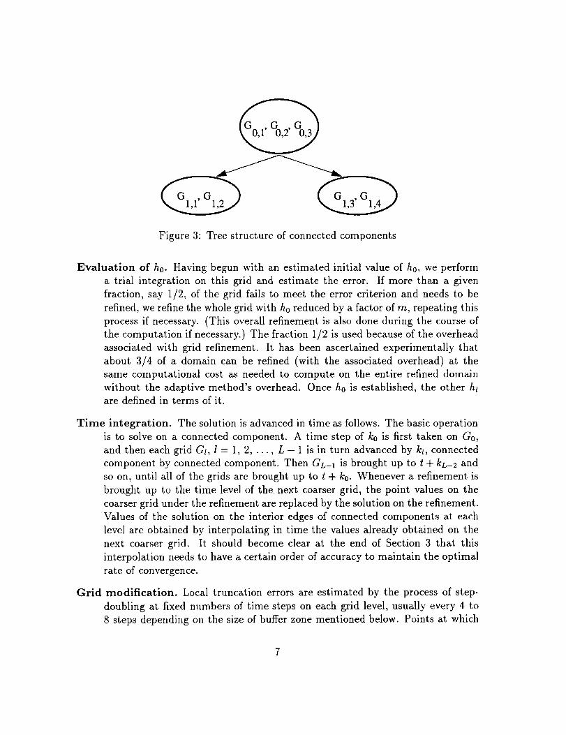
Figure 3: Tree structure of connected components
Evaluation of h0. Having begun with an estimated initial value of h0, we perform
a trial integration on this grid and estimate the error. If more than a given
fraction, say 1/2, of the grid fails to meet the error criterion and needs to be
refined, we refine the whole grid with h0 reduced by a factor of m, repeating this
process if necessary. (This overall refinement is also done during the course of
the computation if necessary.) The fraction 1/2 is used because of the overhead
associated with grid refinement. It has been ascertained experimentally that
about 3/4 of a domain can be refined (with the associated overhead) at the
same computational cost as needed to compute on the entire refined domain
without the adaptive method's overhead. Once h0 is established, the other ht
are defined in terms of it.
Time integration. The solution is advanced in time as follows. The basic operation
is to solve on a connected component. A time step of k0 is first taken on Go,
and then each grid Gl, l = 1, 2, ..., L - 1 is in turn advanced by kl, connected
component by connected component. Then GL-1 is brought up to t + kL-2 and
so on, until all of the grids are brought up to t + k0. Whenever a refinement is
brought up to the time level of the next coarser grid, the point values on the
coarser grid under the refinement are replaced by the solution on the refinement.
Values of the solution on the interior edges of connected components at each
level are obtained by interpolating in time the values already obtained on the
next coarser grid. It should become clear at the end of Section 3 that this
interpolation needs to have a certain order of accuracy to maintain the optimal
rate of convergence.
Grid modification. Local truncation errors are estimated by the process of step-
doubling at fixed numbers of time steps on each grid level, usually every 4 to
8 steps depending on the size of buffer zone mentioned below. Points at which
7

the error criterion is near violation are flagged, clusters of the flagged points are
formed, and refinements overlaying the clusters are constructed. Once a new
component grid is defined, the solution at previously refined points is retained,
and the solution at all other points is obtained by interpolation accurate to a
certain order from the parent grid. (At the initial time, in contrast, the solution
at each refinement level is obtained from the initial data u0.) The refined grids
are constructed with buffer zones around the flagged points, sufficiently wide
so that a phenomenon requiring refinement cannot move out of the refined area
before the next regridding. This is necessary to maintain accuracy. The grids
are moved by constructing a new grid and deleting the old one, see Figure 2.
Each refinement level is in turn refined as necessary in the same manner, until
the finest level has been reconstructed.
3 Stability, Convergence and Error Estimation
3.1 Stability
As mentioned in the beginning of section 2, the original and discretized problems we
deal with are formulated in equations (1)- (3) and equations (4) - (6), respectively.
Once again, we recall that subscripts h and k are used to represent the discretized
domains, operators and variables. Our goal is to use CAG's to compute the solution
such that the error is bounded by a given tolerance ¢, i.e.,
Ileh(T)ll_h <_ (17)
where II. Ilab is some discrete norm and eh(t) is the discrete error function, both tobe defined later.
Before discussing the discrete case, we want to assume that the original initial-
boundary problem is well-posed. The well-poseness of a large class of problems is
discussed in Kreiss and Lorenz [5]. For hyperbolic and parabolic problems, we use
the following definition.
Definition 2: The initial-boundary value problem defined by equations (1) - (3) is
well-posed if there exists an unique solution which satisfies the following estimate
ilu(.,t)ll _ < Ke_t(llu0(.)ll_ + iif(.,.)l _ 2_ I_×[0,,]+ lib(',")110_×[0,,]) (18)
where K and a are constants, t E [0, T] and the norms are defined in the usual way:
Ilu(-,t)ll_ = [ lu(x,t)12dx (19)
/0t/ Ib(x, r)l=ds dr (20)IIb(.,')llo_×[o4 =
f [ If(z,r)12dx dr (21)Ilf(.,.)ll_×[04d0 Jf_
and l" l is the standard L2 norm in R n, i.e., lul2 = u*u.
In order to achieve our goal, some stability results, which are similar to the well-
poseness of the original problem, are needed for the finite difference schemes. In his
report, Pelle Olsson [6] used energy methods and summation by parts (a discrete
version of integration by parts) to establish stability estimates on uniform grids for
the semi-discretized case, i.e., when only the spatial domain is discretized. The spa-
tial discretizations used are centered differences with various orders of accuracy. To
overcome the difficulty of general boundary conditions, some projection matrices are
used so that the solution can be projected into the solution space where the bound-
ary conditions are satisfied. These results hold for a large class of linear problems,
e.g., hyperbolic, parabolic and some mixed types. Although only 2-D problems were
considered in his report, the results can be easily generalized to higher dimensions.
We assume the following stability estimates holds for our finite difference methods on
the uniform mesh. This is consistent with the results of Olsson [6].
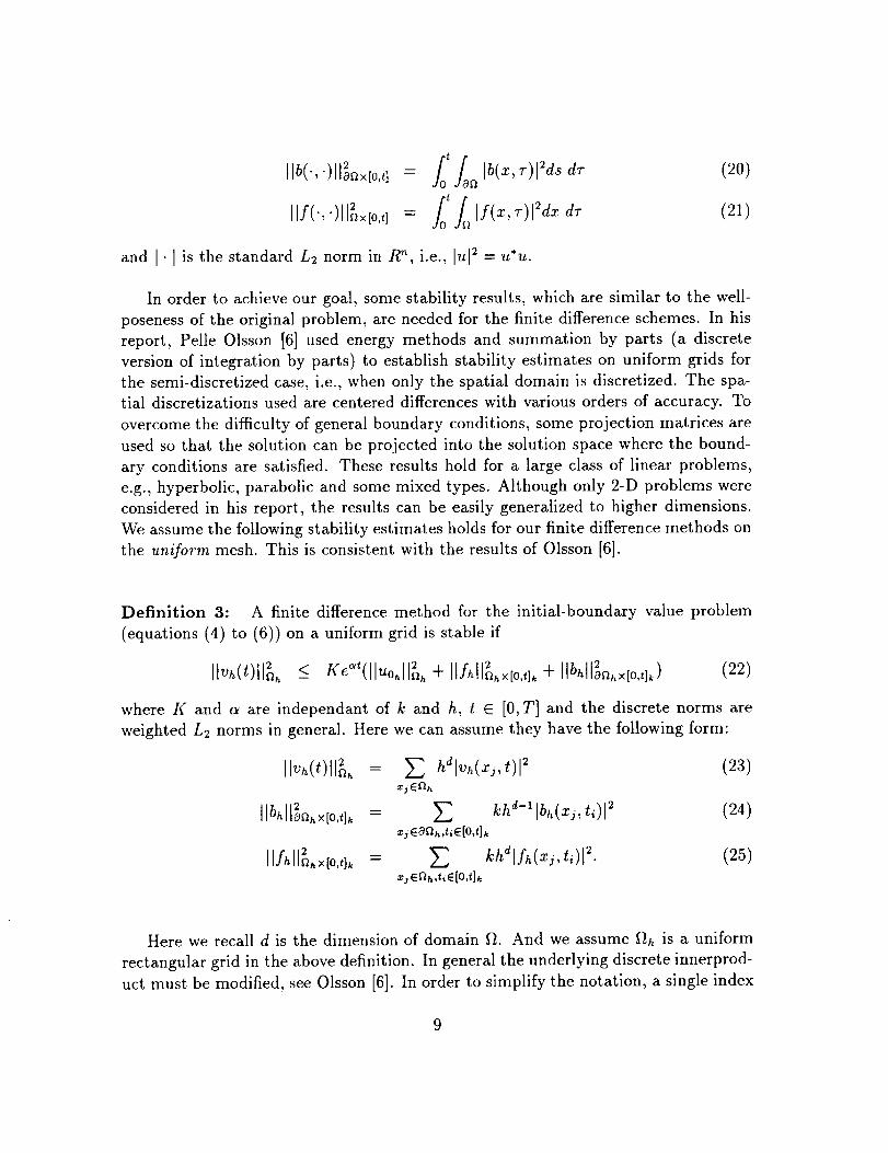
Definition 3: A finite difference method for the initial-boundary value problem
(equations (4) to (6)) on a uniform grid is stable if
_ 2 b 2Ilvh(t)llgh < K_(lluo_llg_ + IIAIl_hx[o4_+ II hlloa.x[o,t],) (22)
where K and a are independant of k and h, t C [0, T] and the discrete norms are
weighted L2 norms in general. Here we can assume they have the following form:
Ilvh(t)ll_%_ = _ halvh(x_,t)l _ (23)xj Eg_h
Ilbhllgahx[o4,= _ khd-'lbh(zj,t,)l _ (24)zj Ea9h,t, e [O,t]k
IlAll%,x[o4_ = _] khdlfh(xj,ti)] 2. (25)xjEt2_,tiE[O,t]k
Here we recall d is the dimension of domain f_. And we assume flh is a uniform
rectangular grid in the above definition. In general the underlying discrete innerprod-
uct must be modified, see Olsson [6]. In order to simplify the notation, a single index

j is used for the grid points in d dimensions. For the same reason, we use the same
K and a in Definition 2 and 3. In fact, they are not necessarily the same constants.
However, in order to approximate the original problem better, it is desirable to have
the a in the discrete case to be close to the one in original problem. This is refered
to as strictly stable in Olsson's report. It can be shown that the two a's are equal up
to an error of order O(h) in his estimates.
Before deriving the error estimates for CAG methods, another assumption is nec-
essary. We will assume K = 1, where K is the coefficient in equation (22). According
to the stability results of Olsson, K > 1. Let's see what happens if K > 1. Since
adaptive grids are used, the stability bound in Definition 3 is used whenever a regrid-
ding process is carried out. We consider a simple case with homogeneous boundary
conditions and zero forcing term. Assume that we regrid at every time step, then we
get
K_kllvh(O)ll_
K2_kllvh(O)ll_
So at time T, the growth bound looks like
[[vh(T)ll_ _ KT/ke_TIIvh(O)I[_
This bound is useless unless K < 1 +O(k). However, we can always absorb K into the
term e_'t with a new a if K < 1 + O(k). Therefore, we take K = 1. Fortunately, many
problems we are interested in have this nice property since they describe physical
phenomena which conserve energy.
3.2 Convergence
Now, we are ready to define _h in the case of CAG's. We use the notation G to
represent this discretization of the original domain. Given a composite component
grid, which is defined in Section 2 and may contain several levels of subgrids, the
domain where the computational solution vector Vh is defined can be constructed in
the following way. Suppose there are L levels of subgrids Go,..., and GL-1, and every
component grid Gl.j is a regular grid. Then Vh is defined spacially on the set
L-2
a= a,_,_,U ( U (a,_,-a,)) (26)1=1
lO
where GI-1 - Gt is the complement operation. This set is well defined in the 1-D
case since we enforce Gt C Gt-1 and there is no overlapping among the subgrids of
the same level. But in higher dimensions there may be overlapping areas in Gl. The
above definition is still valid if the solution vector is uniquely defined on each Gt.
All the components in G_ will have errors of the same magnitude. So the solution
vector can be defined using any one of the grids in the overlapping area. Suppose
Gl,jl, Gtd_, ..., G_,j, have an overlapping area, where jl < j2 < ... < j,_. Then
the solutions of Gl,jl are used in the overlapping area. In other words, by using the
smallest-indexed grid in the overlapping area, we can uniquely define the solution
vector on every level. Then, equation (26) is well defined in higher dimensions and vh
is defined on a piecewise uniform mesh. We also notice that the set G is a function of
time, i.e., G = G(t), because it may change whenever a regridding process is done at
any level. By this observation, we can define Vh on the interval [0, T]. In fact, Vh is a
piecewise constant solution function on [0, T]. Its solution values change only when a
integration or regridding process is carried out at any level. Because G is a piecewise
uniform grid, we can define OG to be the union of all the boundaries of these uniform
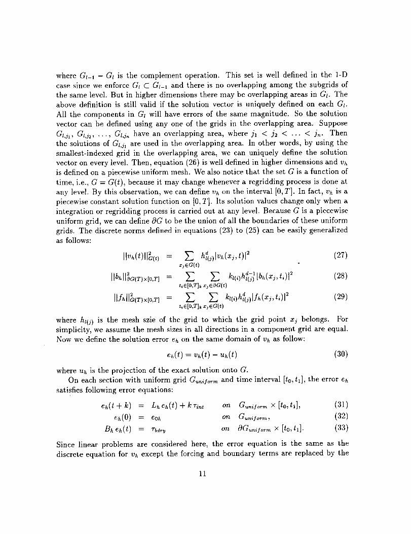
grids. The discrete norms defined in equations (23) to (25) can be easily generalized
as follows:
Ilvh(t)l[_(O = __, hd(j)lVh(Xj,t)l 2 (27)zj • G(t)
2 _ a-1 x (28)libhlt0c<r)×[0,r]- Z _2 k,(,)h,(j)ibh( j,t,)l 2t, •[O,T]k xj COG(t)
i 2 = d (29)Ifhllc(r)×[0,r] _ Z k'(')h'o)lh(x"t')l 2t, •[O,T]k xj •G(t)
where hz(j) is the mesh szie of the grid to which the grid point xj belongs. For
simplicity, we assume the mesh sizes in all directions in a component grid are equal.
Now we define the solution error eh on the same domain of Vh as follow:
_h(t) = vh(t) - uh(t) (30)
where Uh is the projection of the exact solution onto G.
On each section with uniform grid G,,._ilo_m and time interval [to, tx], the error eh
satisfies following error equations:
eh(t + k) = Lh eh(t) + k ri,_, on a_..]o_m × [to, q],
eh(0) = e0h on Gunilorm,
B_eh(t) = _'bd_ on OG_qo.. x [t0,t_].
(31)
(32)(33)
Since linear problems are considered here, the error equation is the same as the
discrete equation for Vh except the forcing and boundary terms are replaced by the
11
local truncation errors. Thus, the growth bound for eh on the piecewise uniform grids
can be obtained by applying the stability results in Section 3.1.
Next we are going to prove the error estimation for CAG methods using induction
on the number of grid levels. First we consider the case of only one level of grids.
Since it is piecewise uniform, we can use the result in equation (22) on each piece
of uniform grid. Also we bound the error on grid G by the summation of the errors
on the pieces of uniform grid because of the way we define G and the norm lI" I la.
Assume the local truncation errors of the numerical method used have the accuracy of
order p at interior and boundary points. The initial values are also assumed accurate
to order p. Then from equation (22), it is easy to see following error bound holds:
II h(T)II Coe Th2op (34)
where _< means "asymptotically less than", since only the leading terms of the trun-cation errors are estimated here.
Now we assume that equation (34) holds for L levels of grids. Next we will show
it for L + 1 levels. Because of the way we construct the subgrids which are nested
in their parent grids, we only need to consider two levels. By induction, we know
the error on the finer of the two levels is of order O(h_), so we can always write it as
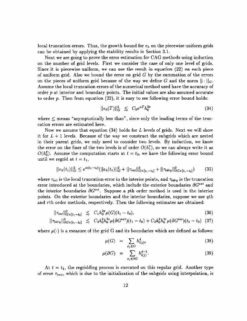
O(h_). Assume the computation starts at t = to, we have the following error bound
until we regrid at t = tl,
Ileh(tx)ll + IIT 'lla×t ,-,0]+ IITbd 2II0a×t,l-,0j) (35)
where ri,_t is the local truncation error in the interior points, and rbd,._, is the truncation
error introduced at the boundaries, which include the exterior boundaries OG _:t and
the interior boundaries OG i'u. Suppose a pth order method is used in the interior
points. On the exterior boundaries and the interior boundaries, suppose we use qth
and rth order methods, respectively. Then the following estimates are obtained:
= (3s)
I_(OG) = E hd(j_ • (39)
I 2I ,.,llcxt,,-,01 (36)2 2r int t¢_ k2h 2q" [_¢_ext_lt to) + C3koh0 _(Oa )( 1 - to) (37)
where #(.) is a measure of the grid G and its boundaries which are defined as follows:
E %,x_EG
xj 60G
At t = tl, the regridding process is executed on this regular grid. Another type
of error n=it, which is due to the initialization of the subgrids using interpolation, is
12

introduced. Let's assumethis processhaserror of O(h_). Thus, after the regridding
process at t = tl, we will have following error estimate:
Ileh(t,+)ll_ < Ileh(t,)ll_ + Ilr_..tll_
< lleh(tl)ll + C4h s. (40)
If equations (35), (36) and (37) are substituted into equation (40), and the fact that
hl/kt = constant is used throughout computation, the total error after the regridding
process at t = tl is
Ileh(tl+)ll_ < + Clh2op#(G)(tl - to) + C2h2o(q+l)#(OGe_t)(tl - to)
+Cah2o(T+')#(OGint)(t, - to)} + C, hg'. (41)
where the subscript + on the left hand side of equations (40) and (41) represents the
fact that the regridding process is done at time t = t,. All the terms in equation
(41) are under control except #(OG {'_t) since we do not know how many subgrids are
generated. The following lemma gives a bound on tt(OGi'_t).
Lemma 1: Let Go be a regular grid in R e. Assume that there are L levels of grids
Go,..., GL-1 with the refinement ratio rn = hj/hj+l. Then the following asymptotic
inequality holds for small h0.
L-1
#(UUOG, d) < holC(d,m,L)#(Go) (42)l=l j
where C(d, m, L) is a constant depending on d, rn, and L.
Proofi Since a regular grid is an union of rectangular grids, without loss of gen-
erality, we can assume that Go is a rectangular grid. First we bound the boundaries
of G1. According to the discussion in section 2, it can be shown that the case with
largest interior boundaries as h0 is very small for d = 2 is in Figure 4. So, it is easy
to see that the following bound holds:
tt([..JOGa,j) _ 2dhao-'tt(G°)j 2dhdo
1 2d= h o _g(Go).
So, for each level l, 1 = 1,2,...,L - 1, we have
1 2d12(UOGI,j) <,_ hl__l--_#(al-1)
J
2d mr1z
13

Figure 4: The casewith largest interior boundariesin 2-D
Therefore,wehave
L-1
,.(U U ac,,_)/=1 j
2d 1 m (m_L_2_< ho'_-_(Co)( +(_)+...+,2d, ,
ho'C(d,m,L)#(Go)
where
241 - (_)--) (43)C(d,m,L)= 2d(1_ _ )
Remark: The above lemma tells us is that, under the worst senerio, the error term
involving #(c3G i'_t) may lose one order of accuracy. However, the bound in the lemma
is very pessimistic. In most situations, the number of subgrids is usually quite small.
So it is very unlikely the term It(c3G mr) will actually change the order of accuracy at
the interior boundaries. Also we see that it is not a good idea to use too many levels
with large mesh ratio, since the constant C in Lemma 1 will be very large when L ism
large and _ > 1.
With this lemma, we can finally bound the error. We notice that for our current
proof, we only need the bound for two level case, i.e.,
2d
i.t(UOG,,j) _ ho'_#(Go). (44)J
Suppose the worst case is considered here, i.e., the refinement and reinitialization
processes are assumed as often as possible. Assuming the time interval is [0, T], then
14

wehavefollowing error bound usingequation (41) and (44):
2s+C3h2o('+')Tho'tL(Go) + C4ho }. (45)
If q = p - 1, r = p, s = p and the initial error is order O(hg), then equation (45) can
be written as
aT p]leh(T)l]a _ CeTh o (46)
where the constant C may depand on L, the number of levels. Therefore, by the
induction argument, we have proved the above error bound for CAD's. Convergence
follows as h0 --* 0 with a fixed maximum number of levels. We have just proved the
following theorem.
Theorem 1: Suppose a well-posed initial-boundary value problem (equations (1) -
(3)) is solved by a numerical method (equations (4)-(6)) using component adaptive
grids with a fixed maximum number of levels of grids. Also assume that the stability
condition (equation (22)) for the numerical method holds on uniform grids, and the
accuracies for the numerical approximations are order p, p- 1, and p on interior points,
exterior boundaries and interior boundaries, respectivelly. Also that the interpolation
process used in the CAG method has accuracy of at least order p. Then the numerical
solution converges to the exact solution in the norm I]" Ila as h0 _ 0, and the order
of convergence is p.
3.3 Error Estimation
From the discussion in Section 3.2, the sources and the magnitudes of various com-
putational errors are well understood. We can implement the numerical method so
that the local truncation error _'i_t in the interior points is dominant. Then
Ileh(T)lla < x/e r (C) T max(Ti ,(x,t))< e. (47)
Therefore, if the bound 5 for the local truncational error satisfies following relation
max(Ti.t(x,t)) < 5 = , (48)_/e "T_u(G) T
then the final error is guaranteed to be bounded by e.
15

Not only can we bound the error, we can also estimate the final error. Since local
truncation errors in all grid points are estimated once every several time steps, simple
quadrature can be used to estimate the final error. In many applications the growth
factor a is not known in advance but it is very easy to approximate a using the
computed solution as the growth factor is asymptotically the same for the solution
and the error.
4 Computational Examples
In this section some numerical experiments in one and two space dimensions are pre-
sented to illustrate component adaptive grid methods and the error bounds derived
in section 3. The programs are written in C because of its capability for dynamic
memory allocation and flexible data structures, which are crucial for our CAG meth-
ods. A SUN Sparcl0 workstation with 96 Mbytes memory is used for both the 1-Dand 2-D cases.
Example 1 (1-D wave equation). In this example, we compute the solution to
the following wave equation in one space dimension.
where
?At _ --U x -_- _U
u(z, O) =0
f(x)k
x E [0,1], t • [0,0.4]
if x • [0,0.211.3 [0.4,1]
if x • (0.2, 0.4)
0.01
f(x) = 50 (0.01 - (x - 0.3) 2 exp( (x - 0.3) 2 - 0.01 )"
The exact solution is a wave front traveling from left to right with speed 1 and growth
rate eat, where a is a constant. Two methods are used to solve this equation: the first
order up-wind method and second-order Lax-Wendroff method. Second order Hermite
interpolation is used with both methods. In Figure 5, we plot the exact solution and
the computational solutions at t = 0.4 with a = 0 using the Lax-Wendroff method
on the coarse grid, 3-level adaptive grids with mesh ratio m = 4 and uniform grid
with mesh size equal to the smallest of the adaptive grids. Both the solutions on the
fine and 3-level adaptive grid are much better than the one on the coarse grid, which
has wiggles at the left corner where the local truncation errors are large. However,
the adaptive grid uses much less time than the uniform fine grid.Next we use the results in section 3 to control the local truncation error tolerance
6 according to the final error bound e. All the computations here are done with
16

0.2
0.15
= 0,1
0.05
o;
0.2
0.15
= 0.1
0.05
06
exact solution
0.5
x
3 level adaptive solution
0.5
x
0.2
0.15
0.1
0.05
0
-0.050
0.2
0.15
= 0.1
0.05
coarse solution (h=O.01)
0.5x
line solution (h=0.01/16)
015x
Figure 5: various computional results to 1-D wave equation at t=0.4
following parameters.
mesh ratio 4
buffer zone width 4 points
regrid every 16 stepscoarse mesh 0.01
CFL No. A 0.9
growth factor a 0final time T 0.36
We collected the data in Tables 1 and 2. In the first column, the final error bounds
are given. The number of levels of adaptive grids used during computation is listed in
the second column. The exact error and estimated error using simple quadrature are
listed in columns 3 and 4, respectively. In the last two columns, we put the running
times for adaptive grids and uniform grids with mesh size equal to the finest mesh
17

size in the corresponding adaptive grids.
Table 1
Results using the up-wind method for the 1-D wave equation
e levels exact II_hlla est. It_hll_ time time using
(sec) fine grid (sec)
5 x 10 -3 1 4.57 x 10 -3 4.54 x l0 -3 0.0 0.0
1 x 10 -3 3 9.37 x 10 -4 9.26 x 10 -4 0.4 4.7
5 x 10 -4 3 3.88 x 10 -4 3.82 x l0 -4 1.0 4.7
1 x 10 -4 4 9.98 x 10 -s 9.90 x 10 -s 12.9 77.0
Table 2
Results using the Lax-Wendroff method for the 1-D wave equation
e levels exact I1_11_ est. II_hll_ time time using
(sec) fine grid (sec)
1 x 10 -3 2 2.08 x 10 -4 1.88 × 10 -4 0.1 0.4
5 x 10 -4 2 1.86 x 10 -4 1.83 x 10 -4 0.1 0.4
1 x 10 -4 3 3.68 x 10 -5 3.81 x 10 -5 0.8 7.0
5 x 10 -s 3 2.24 x 10 -5 2.15 × 10 -5 1.0 7.0
1 x 10 -s 4 7.75 x 10 -6 7.70 x 10 -6 4.6 115.0
5 x 10 -6 4 2.68 × 10 -6 2.60 x 10 -6 10.0 115.0
Several interesting facts are illustrated in Tables 1 and 2. First of all, we see that
our adaptive strategy is very efficient for solving PDE's. It does efficiently generate
different subgrids in response to the final error tolerances. For example, when we use
Lax-Wendroff with tolerance e = 1 × 10 -3 and e = 5 x 10 -4, two levels of grids are
used in both cases. However, in order to satisfy the final error tolerance, the two
Gl's are constructed differently. This is shown in Figures 6 and 7. In the case of
e = 1 × 10 -3, two small subgrids are generated around the two corners where large
local truncation errors appear. When e is reduced to 5 × 10 -4, a large subgrid is
created in G1. The running times in Tables 1 and 2 show that the speedup, i.e., the
ratio between the time using a uniform fine mesh and the time using an adaptive
grid, increases as the final error tolerance is decreased. In other words, our adaptive
strategy is more attractive when high accuracy is needed. This is because only very
18

small regions (the two corners in this example) need to be refined. The data also
illustrate that our simple quadrature error estimation formula gives very satisfactory
results. Of cause, one reason we have such accurate estimates is that the equation has
constant coefficients. A more realistic variable coefficient problem is considered in the
next example. As mentioned in the Section 3, the errors of interpolation and the ones
at boundaries are assumed to be relatively small compared to the local truncation
errors. Now we compute these two types of error explicitly and list them in Tables
3 and 4. To be consistent with the notation used in Section 3, we use Ile .llc to
represent the subgrids' initialization errors caused by interpolation of the coarse grids'
data. ]lei,_tlla and Ilebdrylloa are used to represent the errors caused by local trucation
errors on the interior points, and the errors on both exterior boundaries OG e=t and
interior boundaries OG i'_t, respectively. Indeed, it is shown that Ile .l la and Ilebdr lladare negligible compared to Ile ,lla. Finally we look at error estimation for different
a's, since for some nonlinear problems, the error equations contains non-differentiable
terms. The results for different a's using Lax-Wendroff with tolerance e = 0.0005 are
shown in Table 5. The estimated growth factors are listed in the table. Our error
control and estimation works very well for all three test cases, a = 0, 3 and 6.
GI,1 G1,2I--J t__l
e0,1
Figure 6: Adaptive grid structure for e = 0.001
GI,1i i
e0,1
Figure 7: Adaptive grid structure for e = 0.0005
19

Table 3
Various errors using the up-wind method for the 1-D wave equation
levels exact Ilei_tllc est. [lei_tllc est. Ilebd_yl]0C est. Ile_,,,tllc5 x 10 -3 1 4.57 x 10 -3 4.54 x 10 -3 5.25 x 10 -6 2.13 >( 10 -11
1 × 10⁻³ 3 9.37 x 10⁻⁴ 9.26 X 10 -4 5.55 × 10⁻⁷ 3.27 X 10⁻⁶
5 X 10⁻⁴ 3 3.88 X 10⁻⁴ 3.82 X 10⁻⁴ 7.96 × 10⁻⁷ 9.16 X 10⁻⁷
1 X 10⁻⁴ 4 9.98 X 10⁻⁵ 9.90 X I0-s 6.89 X i0-s 2.41 X 10⁻⁷
Table 4
Various errors using the Lax-Wendroff method to the 1-D wave equation
levels exact Ilehlla est. lle_tllc est. Ilebd,._llOa est. Ile,,_it[la1 x 10-3 2 2.08 × 10⁻⁴ 1.88 x 10⁻⁴ 1.01 x 10⁻⁶ 1.92 × I0-7
5 x 10⁻⁴ 2 1.86 x 10⁻⁴ 1.83 x 10⁻⁴ 1.04 x 10⁻⁹ 7.80 X 10⁻¹²
1 x 10⁻⁴ 3 3.68 x I0-s 3.81 x I0-s 1.43 x 10⁻⁷ 3.17 x I0-7
5 x 10⁻⁵ 3 2.24 × 10⁻⁵ 2.15 × I0-s 7.08 × I0-s 8.(13× I0-s
1 x 10⁻⁵ 4 7.75 x 10⁻⁶ 7.70 x 10⁻⁶ 1.31 x I0-s 1.01 x I0-7
5 x lO-6 4 2.68 x 10⁻⁶ 2.60 x lO-6 4.65 x 10⁻⁹ 4.06 × I0-s
Table 5
Estimates using the Lax-Wendroff methodwith various a's and e = 5 x 10 -4
a estimated a levels exact IlehllG est. Ilehlla0 --1.43 X 10 -4 2 1.86 X 10 -4 1.83 X 10 -4
3 2+2.56X10 -4 3 2.25X10 -4 2.35X10 -4
6 6+4.39x10 -4 4 1.05x10 -4 1.23x10 -4
Example 2 (2-D rotating cone). The rotating cone problem has been used by
Berger and Oliger [2] to illustrate the adaptive grid method using rotated rectangular
subgrids. The problem is
2O

where
ut = yux- xuyS
u(x, O) =0
f(z)I.
x • [-1, 1], y • [-1,1] and t • [0,3.125]
if (x - 0.4) 2 + 1.hy 2 > 0.04
if (x - 0.4) 2 + 1.5y 2 < 0.04
f(x) = 0.25 (1 - 25((x- 0.4) 2 + y2))2.
The solution is a cone with elliptical base which rotates counterclockwise about the
origin. The solution is integrated until the cone is approximately halfway through the
first revolution. The Lax-Wendroff method and second order interpolation are used in
this example. The boundary conditions are zero inflow and first order extrapolation
at outflow. All computations are done with following parameters:
mesh ratio 4
buffer zone width 2 points
regrid every 8 stepscoarse dx 0.05
coarse dy 0.05CFL No. A 0.25
final time T 3.125
Snapshot views of the one subgrid at three intermediate time steps are shown in
Figure 8. We should mention that this example does not fully explore the power of
our stair step subgrids, since the refined regions here are elliptical, which are easily
covered by rectangular grids. We expect our stair step subgrids to be more efficient
when the geometries of subgrids are more complicated. Various computational results
are plotted in Figure 9. It shows that the solution using a coarse grid has lots of
oscillations. They are reduced dramatically if 2 levels of adaptive grids are used. If
we use 3 levels, the oscillations are invisible. Also, we see that the solutions using
adaptive grids are as good as those using uniform grids with the smallest mesh size of
the corresponding adaptive grid, which is shown by their errors (see Table 6). Next,
our error estimation developed in Section 3 is used to approximate various types of
computational errors. The results are listed in Tables 6 and 7.
Since we are solving a variable coefficient problem, the estimated IlehllO is slightly
larger than the exact one. Also, like the 1-D wave equation example, the local trun-
cation error Ilei,_tllG dominates the other two types of error, Ilebd,yl[0a and I[ei,_itlla
(see Table 7). Finally, we estimate the efficiency of our stair step subgrids. We use
21

the two levelcaseasan example. The areaof the subgrid is about 16%of the original
domain. So, the running time on this subgrid is about 167 × 16% = 26.7 (sec). Also,
we know the running time on the coarse grid is 2.7 (sec). Thus, the total time spent
on other things besides integrating the grids is about 31.7 - 26.7 - 2.7 = 2.3 (sec),
which is approximately 8% of the total time for this two level adaptive computation.
This percentage is less than that reported in [2], which was about 12% when using
rotated rectangular subgrids. Like our 1-D example, the 2-D example also shows that
the speedup increases as we decrease the final error tolerance. As mentioned earlier,
we expect our stair step subgrids to be more efficient when refined regions with more
complicated geometries are encountered.
0.8
0.6
0.4
0.2
>- 0
-0.2
-0._
-O.E
-0._
-1-1
t=3.125
I_7
1
t=1.5625
t=O
I I I I I I I I
-0.8 -0.6 -0.4 -0.2 0 0.2 0.4 0.6X
I
0.8
Figure 8: Stair step subgrids for the rotating cone problem
22

0
Y
0
Y
0
Y
exact coarse (dx=dy=O.05)
0.2-,0.1
0
-1
0 -I 0 0 -II 1 I I
x y x
2 level adaptive uniform (dx=dy=O.0125)
-1 0 -11 1 0 1 1 0
x y x
0.2"
-, 0.1.
O.
-1
3 level adaptive uniform (dx=dy=O.O03125)
-1 0 -11 1 0 1 1 0
x y x
Figure 9: Solutions for the rotating cone problem
23

Table 6
Resultsusing the Lax-Wendroffmethod for the 2-D rotating coneproblem
levels exact IJehJJa est. IJehlla time time using exact II_hllc
(sec) fine grid (sec) for fine grid1 x 10 -2 2 5.11 x 10 -3 6.70 x 10 -3 31.7 167.0 5.11 x 10 -3
1 x 10 -3 3 5.32 X 10 -4 7.40 X 10 -4 1024.0 10879.0 5.27 x 10 -4
Table 7
Various errors using the Lax-Wendroff method for the 2-D rotating cone problem
levels exact II_hlla est. It_,lla est. II_ba,_lloa est. II_.lla1 x 10 -_ 2 5.11 x 10 -z 6.70 × 10 -3 4.77 X 10 -6 1.94 × 10 -4
1 × 10⁻³ 3 5.32 × 10⁻⁴ 7.40 × 10⁻⁴ 2.96 x I0-r 2.06 × 10⁻⁵
5 Conclusions
We have presented an algorithm for solving PDE's and estimating the final error
with component adaptive grid methods. Good efficiency of such grids has been illus-
trated in our 2-D example. Applying recent stability results [6] for a class of numerical
methods on uniform grids, we have proven the convergence of these methods for linear
problems on CAG's. We obtain satisfactory final error estimates. Since local trunca-
tion error estimates are obtained during the process of grid refinement, the amount
of extra work to obtain a final error estimate is very small. For linear problems, not
only can the algorithm estimate the final error, it can also be used to control the tol-
erance for the local truncation error in terms of the given final error bound. The next
challenge is to estimate errors for nonlinear problems. Although it is very hard to
establish such results for general nonlinear PDE's, Olsson and Oliger [7] have devised
a technique that makes it possible to obtain energy estimates for initial-boundary
value problems for a class of nonlinear conservation laws. The estimates for finite
difference methods on such nonlinear problems is currently under development. We
think such results will help us estimate and control errors on our CAG's for a large
class of nonlinear problems.
24

Acknowledgment
The authors wish to thank Steve Suhr for some stimulating discussion on the data
structure for the 2-D stair step grids and some figures of composite adaptive grids
used in this paper.
References
[1]
[2]
[a]
[4]
[5]
[6]
[r]
[8]
M. BERGER, Adaptive Mesh Refinement for Hyperbolic Partial Differen-
tial Equations, Ph.D. Thesis, Stanford University, Stanford, CA, 1982
(unpublished).
M. BERGER AND J. OLIGER, Adaptive Methods for Hyperbolic Partial
Differential Equations, J. Comp. Phys., 53 (1984), pp. 484-512.
B. GUSTAFSSON, H.-O. KREISS AND J. OLIGER, Time Dependent
problems and Difference Methods, 1995 (to be published by John Wiley
& Sons).
a. CHESSHIRE AND W. D. HENSHAW, Composite Overlapping Meshes
for the Solution of Partial Differential Equations, J. Comp. Phys., 90
(1990), pp. 1-64.
H. O. KREISS AND J. LORENZ, Initial-Boundary Value Problems and
the Navier-Stokes Equations, volume 136 of Pure and Applied Mathe-
matics, Academic Press, INc, San Diego, CA, 1989.
P. OLSSON, Summation by Parts, Projections and Stability, RIACS
Technical Report 93.04, RIACS, NASA Ames Research Center, Moffett
Field, CA, 1993 (unpublished).
P. OLSSON AND J. OLIGER, Energy and Maximum Norm Estimates for
Nonlinear Conservation Laws, RIACS Technical Report 94.01, RIACS,
NASA Ames Research Center, Moffett Field, CA, 1994 (unpublished).
R. G. VENKATA, J. OLIGER, AND J. H. FERZIGER, Composite Grids
for Flow Computations on Complex 3D Domains, Proc. of the Fifth
SIAM Conf. on Domain Decomp. Methods for Partial Differential Equa-
tions, (1991), pp. 605-613.
25

[9] R. G. VENKATA, Three-dimensional Composite Grid Generation using
Bezier Family of Curves and Surfaces, Second SIAM Conf. on Geom.
Design, (1991).
26