Stability Analysis of an SIR Epidemic Model - Department of

Background InformationNonautonomous to Autonomous

Equilibrium PointReducing SystemStability Analysis

Stability Analysis of an SIR Epidemic Model

Scott Dean, Kari Kuntz,T’Era Hartfield, and Bonnie Roberson

Department of MathematicsLouisiana State University

Baton Rouge, LA

SMILE at LSU, July 2009

Scott Dean, Kari Kuntz, T’Era Hartfield, and Bonnie Roberson Stability Analysis of an SIR Epidemic Model



IntroductionBackground

Introduction

The SIR epidemic model is a dynamical system, as it canvary with respect to time for up to all three variablesWhen conducting a stability analysis, we ask the followingquestions:Are there any constant solutions?If so, do solutions near the constant move toward or awayfrom the constant solution?What happens to solutions as t approaches infinity?Do any solutions oscillate?





Introduction

If there is a constant solution, the phase portarait of thedynamical system will either show the solutions havingvectors tending either toward or away from the equilibriumvalue.If the values of the system near the equilibrium value alltend toward the point, the equilibrium point is consideredstable, or an attractor.If the values of the system near the equilibrium value alltend away from the value, then the point is consideredunstable, or a repelling point.In some cases, some values tend toward the equilibriumpoint, and some tend away from it. This is called a saddlepoint. It is unstable.





Introduction

Yet other cases show an equilibrium point at the origin, butall trajectories near the equilibrium point stay a smalldistance away. This is a stable equilibrium point, but it isnot globally asymptotically stable.The case where both eigenvalues are real, negative, anddistinct produces a phase portrait that shows alltrajectories tending toward the equilibrium point as t →∞,the value of x(t) gets small, so it is a globally stableequilibrium point.When both eigenvalues are real, negative, and equal, thephase portrait shows a globally stable equilibrium point ifthe two eigenvectors are linearly independent.





Introduction

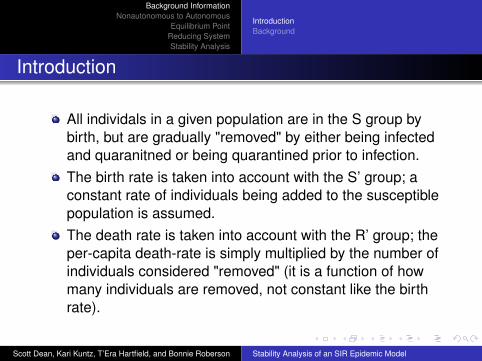
All individals in a given population are in the S group bybirth, but are gradually "removed" by either being infectedand quaranitned or being quarantined prior to infection.The birth rate is taken into account with the S’ group; aconstant rate of individuals being added to the susceptiblepopulation is assumed.The death rate is taken into account with the R’ group; theper-capita death-rate is simply multiplied by the number ofindividuals considered "removed" (it is a function of howmany individuals are removed, not constant like the birthrate).





Introduction

The model takes into account the fact that not all contactsbetween the susceptible group and the infectious groupare "adequate contact" or sufficient to cause infection.The "basic reproduction ratio" b

g gives the researcher anidea of how the epidemic will progress:If it is greater than 1, the number of individuals infected isgreater than the number of individuals recovering, so thedisease will continue to spread.If it is less than (or equal to) 1, the number of individualsrecovering is greater than the number of individualsinfected, so the disease will spread more slowly.This is a very important parameter in epidemiology.





Introduction

N is a constant; it is the total number of the population. Thederivative of N is zero. This is very important for solving thesystem of differential equations 0 = S′ + I′ + R′.The initial value of t is zero, but for the stability analysis weassume t to be the open interval in the neighborhood of(0,0).GLOBAL ASYMPTOTIC STABILITY: Equlibrium values forthe system approach the same value from all sides whenlooking at the phase portrait of the dynamical system.Phase portrait: a "sketch" of the trajectories of a dynamicalsystem, showing the direction of the motion of thepoint(x,y) as t increases. The direction is indicated by the

velocity vectordxdtdydt

.





Introduction

Why do we use this model?Epidemiologists use this model because it allows moreflexibility than the logistic model, which allows for onlydiffering birth and death rates.It allows the ability to form conclusions regarding thelikelihood of a contact resulting in an infection (which tellsresearchers how quickly people move from the S group tothe I group).Researchers can also observe the rate where people movefrom the I group to the R group, showing how quicklyindividuals move from "infectious" to "removed".Once an individual moves into the R group, he or she isincapable of being reinfected or infecting others.





Introduction

An example of this scenario is smallpox:every person born (prior to being innoculated, which is notconsidered here) is equally prone to infection, so includedin the S group.Once an individual is in the I group, or infectious, they arecapable of spreading the disease to others based on thebasic reproduction ratio.They remain in the I group until they either recover (g) ordie (m), both of which occur proportionally to the number ofpeople in the I group.Those that are quarantined either before or after infection,and are thus not able to be part of the I class bycontributing to the infection of others, are consideredremoved, or are in the R group.The sum of these three groups comprises the entirepopulation N, which is a positive constant. Once a personis removed, dies, or recovers, he or she is incapble ofcatching or transmitting the disease again.





Project Goal

To properly understand the behavior of the SIRmodel we must first perform a complete stabilityanalysis of the model. This task includes:• finding the limit system• finding upper and lower bounds of the

system• finding an equilibrium point• applying appropriate theorems to determine

local or global stabilityScott Dean, Kari Kuntz, T’Era Hartfield, and Bonnie Roberson Stability Analysis of an SIR Epidemic Model




Project Goal

We must also determine whether theequilibrium point is stable or asymptoticallystable.For our model, we found that the system isglobally asymptotically stable.





Background Information

Consider the model

S′(t) = Λ− βS1N− µS

I′(t) = βS1N− (µ+ γ)I

R′(t) = γI − µR,

where

N(t) = S(t) + I(t) + R(t).




IntroductionLimit SystemLower BoundUpper BoundConfirmation

To perform the stability analysis of our system, we will employan autonomous system instead of the nonautonomous systemwe were given.

DefinitionConsider the following systems:

d(X )

dt= F (t ,X ) (1)

d(Y )

dt= G(X ) (2)

Equation 1 is called asymptotically autonomous with the limitsystem, Equation 2, if F (t ,X )→ G(X ) as t →∞ for X in Rn.





Limit System

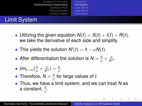
• Utilizing the given equation N(t) = S(t) + I(t) + R(t),we take the derivative of each side and simplify.

• This yields the solution N ′(t) = Λ− µN(t).

• After differentiation the solution is N = Λµ

+ ceµt .

• limt→∞( Λµ

+ ceµt ) = Λ

µ.

• Therefore, N = Λµ

for large values of t .• Thus, we have a limit system, and we can treat N as

a constant, Λµ.





Lower Bound

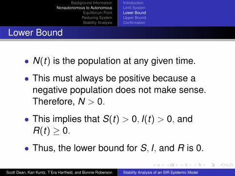
• N(t) is the population at any given time.

• This must always be positive because anegative population does not make sense.Therefore, N > 0.

• This implies that S(t) > 0, I(t) > 0, andR(t) ≥ 0.

• Thus, the lower bound for S, I, and R is 0.





Upper Bound

• To find the upper bound of the system, wewill use the limit system found earlier.

• As discussed earlier N can now be treatedas a constant, N = Λ

µ , for large values of t .

• However, for other values of t , N = Λµ + c

eµt .

• S, I, and R are separately ≤ N.• Therefore, S, I, and R ≤ Λ

µ + ceµt .





Confirmation

• We have found the limit system for themodel.

• We have found the lower bound (S, I, and R> 0) and the upper bound (S, I, andR ≤ Λ

µ + ceµt ).

• We can now apply the following Theorem :





Theorem

d(X )

dt= F (t ,X ) (3)

d(Y )

dt= G(X ) (4)

where Equation 4 is the limit system of Equation 3.

TheoremIf solutions of Equation 3 are bounded and the equilibrium X ofEquation 4 is globally asymptotically stable, then any solutionX(t) of Equation 3 satisfies X (t)→ X as t →∞.

Therefore, we may now consider only the limit system.




Equilibrium Point

We now need to find the equilibrium points forthese equations.

DefinitionGiven an equation dx

dt = f (x), a point x∗ is an equilibriumpoint if f (x∗) = 0.




Equilibrium Point

We can get the equilibrium points by setting the equations in

the model equal to zero and solving the system for S, I, and R.

By doing so, we obtain:

S =Λ2

µ(β + Λ)

I =βΛ

(β + Λ) + (µ + γ)

R =γβΛ

µ(β + Λ)(µ + γ).




Equilibrium Point

We know that this is the only equilibriumpoint because the equation for S is linear.Therefore, the equilibrium point is:

(Λ2

µ(β + Λ),

βΛ

(β + Λ) + (µ + γ),

γβΛ

µ(β + Λ)(µ + γ)).




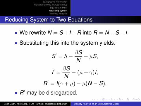
Reducing System to Two Equations

• We rewrite N = S + I + R into R = N−S− I.

• Substituting this into the system yields:

S′ = Λ− βSN− µS,

I ′ =βSN− (µ + γ)I,

R′ = I(γ + µ)− µ(N − S).

• R′ may be disregarded.




The Set UpSpecified Lyapunov FunctionStability

Now that we have simplified our system down totwo autonomous equations,

S′(t) = Λ− βS1N− µS

andI ′(t) = βS

1N− (µ + γ)I,

we can analyze the stability using the properLyapunov function.





Lyapunov Function

DefinitionA function V (x , y) is said to be positive definite on a region Dcontaining the origin if for all (x , y) 6= (0,0), V (x , y) > 0.V (x , y) is said to be negative definite on a region D containingthe origin if for all (x , y) 6= (0,0), V (x , y) < 0.

DefinitionA function V (x , y) is said to be a Lyapunov Function on anopen region D if the function is continuous, positive definite,and has continuous first-order partial derivatives on D.





Theorem

TheoremIf there exists a Lyapunov function V (x , y), dependent on asystem dx

dt = f (x , y) and dydt = g(x , y) with equilibrim point

(x , y) = (0,0), and dVdt is negative definite on an open region D

containing the origin, then the zero solution of the system isasymptotically stable.

When D encompasses all possible values of (x , y) and followsall of the specified criteria above, the projected stability of thesystem is said to be global.





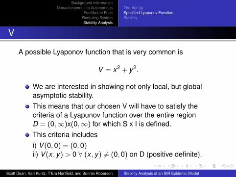
V

A possible Lyaponov function that is very common is

V = x2 + y2.

We are interested in showing not only local, but globalasymptotic stability.This means that our chosen V will have to satisfy thecriteria of a Lyapunov function over the entire regionD = (0,∞)x(0,∞) for which S x I is defined.This criteria includesi) V (0,0) = (0,0)ii) V (x , y) > 0 ∀ (x , y) 6= (0,0) on D (positive definite).





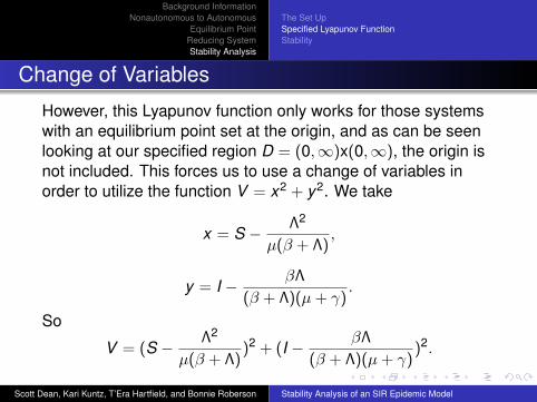
Change of Variables

However, this Lyapunov function only works for those systemswith an equilibrium point set at the origin, and as can be seenlooking at our specified region D = (0,∞)x(0,∞), the origin isnot included. This forces us to use a change of variables inorder to utilize the function V = x2 + y2. We take

x = S − Λ2

µ(β + Λ),

y = I − βΛ

(β + Λ)(µ+ γ).

So

V = (S − Λ2

µ(β + Λ))2 + (I − βΛ

(β + Λ)(µ+ γ))2.





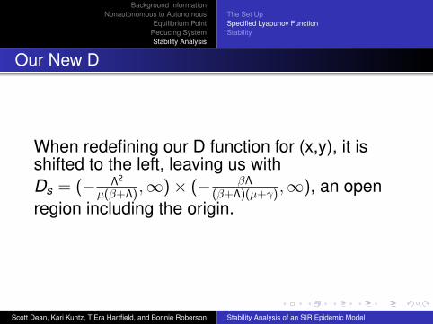
Our New D

When redefining our D function for (x,y), it isshifted to the left, leaving us withDs = (− Λ2

µ(β+Λ) ,∞)× (− βΛ(β+Λ)(µ+γ) ,∞), an open

region including the origin.





We now check the derivative of our V:

dVdt

=∂V∂S

dSdt

+∂V∂I

dIdt

= −2[(µ(β + Λ)

Λ2 )(S− Λ2

µ(β + Λ))2+(

(β + Λ)(µ+ γ)

βΛ)(I− βΛ

(β + Λ)(µ+ γ))2].

The overall sign of dVdt is determined by the factor of -2 outside

the brackets.

Furthermore, the only point that will make this equation equal tozero is the equilibrium point (x , y) = (0,0), which corresponds tothe values S = Λ2

µ(β+Λ) and I = βΛ(β+Λ)(µ+γ) .





Global Asymptotic Stability

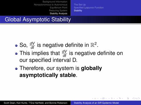
So, dVdt is negative definite in R2.

This implies that dVdt is negative definite on

our specified interval D.Therefore, our system is globallyasymptotically stable.


Documents

Stability Analysis of an SIR Epidemic Model - Department of