Applied Mathematics, 2013, 4, 109-117 http://dx.doi.org/10.4236/am.2013.410A2011 Published Online October 2013 (http://www.scirp.org/journal/am)

Copyright © 2013 SciRes. AM

Global Stability Analysis of a Delayed SEIQR Epidemic Model with Quarantine and Latent

Tiantian Li, Yakui Xue* Department of Mathematics, North University of China, Taiyuan, China

Email: *xyk5152@163.com

Received June 12, 2013; revised July 12, 2013; accepted July 19, 2013

Copyright © 2013 Tiantian Li, Yakui Xue. This is an open access article distributed under the Creative Commons Attribution Li- cense, which permits unrestricted use, distribution, and reproduction in any medium, provided the original work is properly cited.

ABSTRACT

In this paper, we study a kind of the delayed SEIQR infectious disease model with the quarantine and latent, and get the threshold value which determines the global dynamics and the outcome of the disease. The model has a disease-free equilibrium which is unstable when the basic reproduction number is greater than unity. At the same time, it has a unique endemic equilibrium when the basic reproduction number is greater than unity. According to the mathematical dynamics analysis, we show that disease-free equilibrium and endemic equilibrium are locally asymptotically stable by using Hurwitz criterion and they are globally asymptotically stable by using suitable Lyapunov functions for any . Besides, the SEIQR model with nonlinear incidence rate is studied, and the 0 that the basic reproduction number is a

unity can be found out. Finally, numerical simulations are performed to illustrate and verify the conclusions that will be useful for us to control the spread of infectious diseases. Meanwhile, the 1,k 3k will effect changing trends of ,S ,E ,I

,Q R in system (1), which is obvious in simulations. Here, we take 3k as an example to explain that.

Keywords: SEIQR Model; Lyapunov Function; Delay; Global Stability; Nonlinear Incidence Rate; Simulations

1. Introduction

Many people have been paying attention to the study of some epidemics, and have accumulated a lot of experi- ence. By establishing reasonable mathematical models, they put forward the measures which controlled the spread of epidemics effectively. And many scholars re- searched specific diseases and considered the diseases with incubation period, recovery time, quarantine and so on [1-6]. So many epidemics were controlled. Generally speaking, when epidemics spread, there are many kinds of delays, which include immunity period delay [7-9], infectious period delay, incubation period delay. In [10], Enatsu et al. studied stability analysis of delayed SIR epidemic models with a class of nonlinear incidence rates, at the same time, they proved disease-free equilibrium was globally asymptotically stable and endemic equilib- rium was permanent under certain conditions. At the same time, global stability of an SIR (where S, I, R de- note the number of susceptible individuals, infectious individuals, recovery individuals) epidemic model with constant infectious period was studied by Zhang et al.

[11], they showed the endemic equilibrium was globally asymptotically stable with appropriate Lyapunov func- tions. And in [12], Gao et al. discussed pulse vaccination of an SEIR (E denote the number of exposed individuals) epidemic model with delay and bilinear incidence. Mean- while, impulsive vaccination of SEIR epidemic model with time delay and nonlinear incidence rate was re- searched by Zhao et al. [13], and showed the pulse sys- tem that was similar to the pulse system with bilinear incidence rate. Besides, on the basis of [13], Xu and Ma introduced the saturated incidence rate. Meanwhile, they showed disease-free equilibrium and endemic equilib- rium were globally asymptotically stable under certain condition in [14]. However, in addition to the bilinear incidence rate, nonlinear incidence rate and saturated in- cidence rate, there were some scholars who studied the non-monotone incidence. For example, an SIRS epide- mic model with pulse vaccination and non-monotonic in- cidence rate was discussed by Zhang et al. [15], and they proved the disease-free equilibrium and endemic equilib- rium were asymptotically stable under certain conditions. Besides, some scholars studied a delayed SEIQR (Q de- note the number of quarantined individuals) epidemic *Corresponding author.

T. T. LI, Y. K. XUE

Copyright © 2013 SciRes. AM

110

model with pulse vaccination and the quarantine measure, and they showed that the disease-free equilibrium of the system was globally attractive and endemic equilibrium was permanent under certain conditions. In this paper, we study a delayed SEIQR epidemic model without pulse on the basis of [14,16].

The organization of this paper is as follows: In Section 2, SIQR epidemic model and its basic reproduction number and existence of equilibrium are given. In Sec- tion 3, the local stability of endemic equilibrium and disease-free equilibrium is showed by using Hurwitz criterion. By using suitable Lyapunov functions and La- Salle’s invariance principle, we prove the disease-free equilibrium is globally asymptotically stable when the basic reproduction number is less than unity and the en- demic equilibrium is globally asymptotically stable when the basic reproduction number is greater than unity. At the same time, the system with the nonlinear incidence rate is discussed in Section 3. In Section 4, presents the numerical simulations of the system followed by a con- clusion in Section 3. At last, a brief discussion is given in Section 5 to conclude this work.

2. Establishment of the Model

We establish the following SEIQR epidemic model, Here S t represents the number of individuals who are sus-

ceptible to disease, that is, who are not yet infected at time t. E t is the number of individuals who are in- fected but hardly infectious. So we think they can’t infect other people, but they need to be quarantined. I t re- presents the number of infected individuals who are in- fectious and are able to spread the disease by contact with susceptible individuals. Q t is the number of in- fectious individuals who are quarantined at time t. R t represents the number of recovered individuals at

time t.

2

2

1

2 1 3

3 2

1 2 4

3 5

d,

d

de ,

d

de ,

d

d,

d

d.

d

SA S SI

t

ESI S t I t k k E

t

IS t I t k I

t

Qk E k I Q

t

RQ I k E R

t

(1)

The initial conditions for system (1) are

1 2 3

4 5

5

5

, , ,

, , 0, ,0 ,

0 0, ,0 , , 1, 2,3, 4,5.

: 0 .

i

i i

S E I

Q R

C h i

x x

And the feasible region of the model with the initial conditions above is

51 +, , , , .

AS E I Q R S E I Q R

Here, we presume that

1 2 3 4 5min , , , , .

It is easy to show that 1 is positively invariant with respect to system (1).

Where all the parameters are positive constants, A is the recruitment rate of the susceptible population, 1 ,

2 , 3 , 4 , 5 are the natural death rate of the susceptible, exposed, infectious, quarantine and recov- ered respectively, is the disease transmission coeffi- cient, 1 is the death rate due to disease without quar- antine, 2 is the death rate due to disease after quar- antine, is the recovery rate after quarantine, is the recovery rate without quarantine, 1k , 2k are quarantine rate of E , I respectively, 3k is the re- covery rate of E and is the latent period of the epi- demic.

Because the variables R and Q do not appear in the first three equations in system (1), we further simplify system (1) and then obtain the following model

2

2

1

2 1 3

3 2

d,

dd

e ,dd

e .d

SA S SI

tE

SI S t I t k k EtI

S t I t k It

(2)

In this paper, we are concerned with system (2). The initial conditions for system (2) are

1 2 3

3

3

, , , 0,

,0 , 0 0, ,0 , , 1,2,3.

: 0 .

i

i i

S E I

C h i

x x

And the feasible region of the model with the initial condition above is

32 +, , .

AS E I S E I

Here, we presume that

T. T. LI, Y. K. XUE

Copyright © 2013 SciRes. AM

111

1 2 3min , , .

It is easy to show that 2 is positively invariant with respect to system (2).

According to the practical significance of the epidemic model, system (2) always has a disease-free equilibrium

01

,0,0 .A

E

Denote the basic reproduction number of system (2)

2

01 3 1 2

e.

AR

k

Define 3 1 2 .a k If the basic reproductive number 0 1,R system (2) has an unique endemic equi- librium

2 2

2 2

*

* 1

2 1 3

1 e e, , .

e e

a I A aaE

ak k

3. The Stability of Equilibrium

In this section, we discuss the local stability of endemic equilibrium and disease-free equilibrium of system (2) by analyzing the corresponding characteristic equations re- spectively. By defining reasonable Lyapunov functions, we resolve the global dynamics of equilibriums without requiring any extra conditions. In addition, system (2) with nonlinear incidence is studied.

3.1. Stability of Disease-Free Equilibrium

Theorem 3.1.1. If 0 1R , the disease-free equilibrium

0E of system (2) is locally asymptotically stable for any in 2 . If 0 1R , it is unstable for any in

2 . Proof. The characteristic matrix at the disease-free equi-

librium 0E

2

0

2

11

2 11 1

1

0

e e0 .

e e0 0

E

A

A AJ k

Aa

When 0, the characteristic equation at the dis-ease-free equilibrium 0E of system (2) takes the form

2

1 2 11

e e0.

Ak a

Clearly, system (2) always has two negative real roots

1 1 2 2 1, .k

All other roots are given by the roots of equation

2

1

e e0,

Aa

2 Re

1

e e cos lmRe .

Aa

Assume Re 0, 2

1

eRe .

Aa

That is, 0Re 1 .a R Because 0 1,R Re 0, which is contradictory.

So Re 0, Therefore the disease-free equilibrium

0E of system (2) is locally asymptotically stable. If 0 1,R let

2

1

e e,

0 0, 0,

Af a

f f

so there is a positive real root at least. The disease-free equilibrium 0E of system (2) is unstable.

When 0, it is easy for us to prove the disease-free equilibrium 0E of system (2) is locally asymptotically stable.

Theorem 3.1.2. If 0 1R , the disease-free equilib- rium 0E of system (2) is globally asymptotically stable for any in 2 .

Proof. For 0,t define a differentiable Lyapunov function

1 2.V V V

2

1

2

,

e d .t

t

V I

V S I

Obviously, 1 2 0.V V V Calculating the derivative of V t along positive so-

lutions of system (2), it follows that

21 2 e .V V V SI aI

According to the feasible region, .A

S

So

2

1

e.

AV a I

That is,

0 1 .V a R I

And when 0 1, 0.R V While 0,V if and only if,

T. T. LI, Y. K. XUE

Copyright © 2013 SciRes. AM

112

, 0, 0.S A E I

For all t, it is easy to show that 0E is the largest in- variant subset of the set , , : 0 .S E I V Because of LaSalle’s invariance principle, disease-free equilibrium

0E of system (2) is globally asymptotically stable. This completes the proof.

3.2. The Stability of Endemic Equilibrium

Theorem 3.2.1. For any , if 0 1,R the endemic equilibrium *E of system (2) is locally asymptotically stable in 2.

Proof. The characteristic matrix at the endemic equi- librium *E

2 2*

2 2

* *1

* * * *2 1

* *

0

e e e e .

e e 0 e eE

I S

J I I k S S

I a S

Order * *, .I b S c The characteristic equation at the endemic equilibrium *E is

2 2

2 1

1 e e e e 0.

k

b c a bc

Clearly, system (2) always has a negative real root

2 1 .k

When 0, all other roots are given by the roots of equation

1 0.b c a bc

,a c so

1 10, 0.a b c bc b a c

So according to Hurwitz criterion, the endemic equi- librium *E of system (2) is locally asymptotically sta- ble.

When 0, all other roots are given by the roots of equation

2 21 e e e e 0.b c a bc

Simplify, we can get

221 1 1e e 0.a b c a b

Let

1 1

2 1

,

.

m a b

m a b

Then

221 2 1e e 0.m m c (3)

Let i is the root of Equation (3), on substitut- ing to i Equation (3), we derive that

221 2 1e

cos sin 0.

m i m c i

i

Separating real and imaginary parts, it follows that

2 2

2 2

22 1

1 1

e cos e sin 0,

e cos e sin 0.

m c c

m c c

2

2

32 1 1

2 21

21 1 1 2

2 21

sin ,e

cos .e

m m

c

m m

c

Then we can get

2

2

2

2 26 2 41 1 2 1 1

2 22 2 22 1 1 2 1 1 1 1

22 2 2 42 1 1

2 e

2 2 e

e 0.

m m m c

m m m m c

m c

Order

2

2

2

2 221 1 1 2 1 1

2 22 22 2 1 1 2 1 1 1 1

22 2 2 43 2 1 1

2 e ,

2 2 e ,

e .

f m m m c

f m m m m c

f m c

Letting 2 ,z then Equation (4) becomes 3 2

1 2 3 0.z f z f z f

Here

2 2

2 2

2 21 1 1

2 22 2 22 1

2 2 2 21 1 1

23 1 2 1

2 2 0,

e 2 e

( 2 ) 0,

( e ) e 0.

f b b

f b c b c

a b b

f m c bc

　　　

Application of the conclusions of [17], we can know that positive z doesn’t exist. Hence also doesn’t exist. There are not pure imaginary roots in system (2). Therefore all the roots have negative real component. So endemic equilibrium *E of system (2) is locally asymp- totically stable.

T. T. LI, Y. K. XUE

Copyright © 2013 SciRes. AM

113

Theorem 3.2.2. If 0 1,R when 0, the endemic equilibrium *E of system (2) is globally asymptotically stable in 2.

Proof. Define a differentiable Lyapunov function

1 2.V V V

* *1 1 *

* *2 2 *

ln ,

ln .

SV S S S

S

IV I I I

I

1 20, 0, both of them are real numbers. The func- tion is positive definite. Calculating the derivative of V along positive solutions of system (2), it follows that

1 2.V V V

On substituting * * * *1 , ,A S S I a S we have

2*1* * *

1 1 1 1 1 1 1

2* *

* * *1 1 1 1 2 2

* * *2 2 .

SV S S I S SI

S

S IS S I SI S I

S

SI S I

Let 1 2 . So 0.V In addition, when 0,V if and only if

* * *, , .S S E E I I It is easy to show that *E is the largest invariant sub-

set of the set , , : 0 .S E I V Because of LaSalle’s invariance principle, the endemic equilibrium *E of system (2) is globally asymptotically stable when 0 . This completes the proof. Theorem 3.2.3. If 0 1,R when 0, the endemic

equilibrium *E of system (2) is globally asymptotically stable in 2.

Proof. For 0,t define a differentiable Lyapunov function

1 2.V V V

Order

2* * * *1 1 2* *

* * * *2 2 * *

ln e ln ,

ln d .t

t

S IV S S S I I I

S I

S IV S I S I S I

S I

1 20, 0, both of them are real numbers. Let * * * *

1 , .A S S I a S

Then the derivative of V along the solution of sys- tem (2) satisfies

** * *1

1 1 1 1 1

2* *1 *

1 2

*2* * *

2 2

2 2

* *2

2

ln .

SV S S S I SI

S

S IS I S t I t

S

S t I t IS I S I

I

SI S t I t

S t I tS I

SI

** 1

1 12 0.S

S SS

Then

2* *1* *

1 1

* * *1 2 2 *

*2* *

2

2* **2* * * *

2 2*

2* *2* *

2

ln

ln

2 .

S IV S I SI

SS t I t

S I SI S IS I

I S t I tS I

I

S ISS I S I

SI

S IS I

S

Simplify, we can get

* *2 2 1 1

2* *2 * *

2

2* *1* *

1 .

V S S S S I

S IS I

S

S IS I

S

Order 2 1, 0.V Besides, when 0,V if and only if * * *, , .S S E E I I

It is easy to show that *E is the largest invariant sub- set of the set , , : 0 .S E I V Because of LaSalle’s invariance principle, the endemic equilibrium *E of sys- tem (2) is globally asymptotically stable when 0 . This completes the proof.

3.3. The SEIQR Epidemic Model with Nonlinear Incidence Rate

Zhao et al. studied delay SEIR epidemic model with the nonlinear incidence rate like pS I in the case of pulse. In this paper, the model without pulse is discussed.

T. T. LI, Y. K. XUE

Copyright © 2013 SciRes. AM

114

2

2

1

2 1 3

3 2

1 2 4

3 5

d,

dd

e ,dd

e ,dd

,dd

.d

p

p p

p

SA S S I

tE

S I S t I t k k EtI

S t I t k ItQ

k E k I QtR

Q I k E Rt

It is easy to show disease-free equilibrium is globally asymptotically stable, endemic equilibrium is locally asymptotically stable. The ways we use are similar to that in system (1), here they are omitted.

4. The Numerical Simulations

In this section, we study system (1) numerically. Ac- cording to the different datas that can reflect the actual situation, we get the different simulation images to prove our conclusions obviously (Figures 1-9).

Here, according to the different actual situations, while take different parameters, we can get different simulation diagrams of the disease-free equilibrium. At the same time, we find out the disease will die out after much more time when 0R increases. For example,

1 2 3

4 5 1 2 1

2 3

0.2, 1, 0.1, 0.15, 0.2,

0.05, 0.06, 0.4, 0.2, 0.3,

0.8, 0.2, 0.5, 0.3, 3.

A

k

k k

　 　 　 　

　

　 　 　 　

Here 0 0.7502,R see Figure 1.

1 2 3 4

5 1 2 1 2 3

0.2, 1, 0.05, 0.1, 0.2, 0.05,

0.06, 0.4, 0.2, 0.3, 0.8, 0.2,

0.5, 0.3, 10.

A

k k k

　 　 　 　 　

　 　 　 　 　

　 　

Figure 1. Simulation diagram of the disease-free equilib- rium when 0 0.7502R .

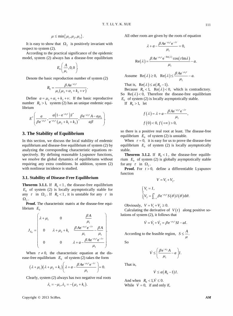
Figure 2. Simulation diagram of the disease-free equilib- rium when 0 0.8656R .

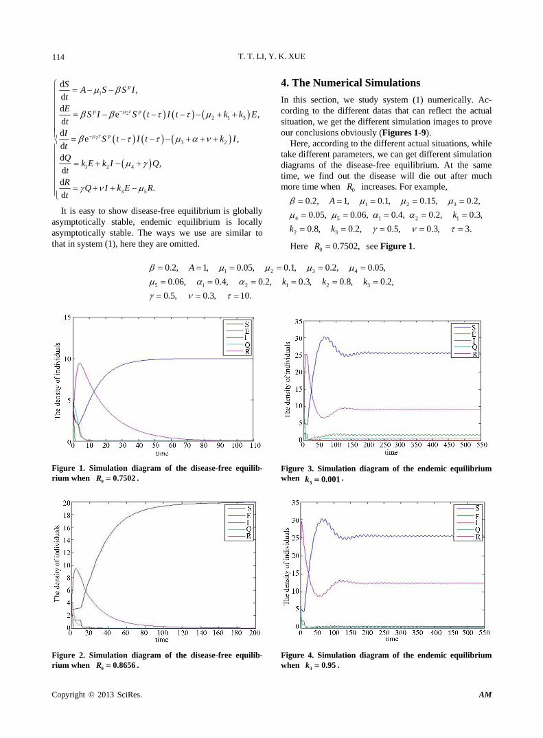
Figure 3. Simulation diagram of the endemic equilibrium when k3 0.001 .

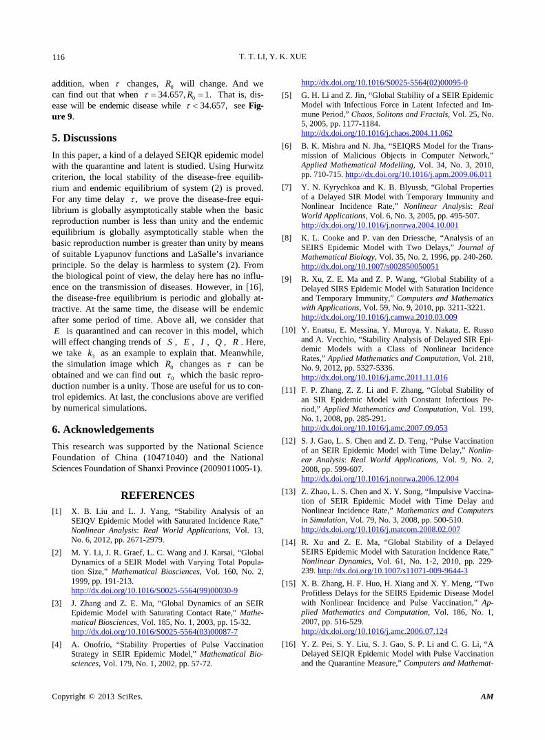
Figure 4. Simulation diagram of the endemic equilibrium when 3 0.95k .

T. T. LI, Y. K. XUE

Copyright © 2013 SciRes. AM

115

Figure 5. Simulation diagram of the endemic equilibrium when 0 31.6816R .

Figure 6. Simulation diagram of I when 0 31.6816R .

Figure 7. Simulation diagram of E when 0 31.6816R .

Here 0 0.8656,R see Figure 2. When take different 3k , we can get different simula-

tion images. In other words, the R increases when 3k increases, which is obvious in Figures 3 and 4. And then it is easy for us to find that how 3k effects changing trends of S , E , I , Q , R .

Figure 8. Simulation diagram of I when 3 .

Figure 9. Simulation diagram of basic reproduction num- ber.

1 2 3

4 5 1 2 1

2 3

0.2, 2, 0.04, 0.1, 0.2,

0.05, 0.06, 0.4, 0.2, 0.3,

0.6, 0.001, 0.7, 0.5, 11.

A

k

k k

Here 0 1.9 ,581R see Figure 3.

1 2 3

4 5 1 2 1

2 3

0.2, 2, 0.04, 0.1, 0.2,

0.05, 0.06, 0.4, 0.2, 0.3,

0.6, 0.95, 0.7, 0.5, 11.

A

k

k k

Here 0 1.9 ,581R see Figure 4. At last, if the basic reproduction number is much lar-

ger and we will get new diagrams. For example, let

1 2 3

4 5 1 2 1

2 3

0.8, 2, 0.04, 0.1, 0.1,

0.05, 0.06, 0.05, 0.2, 0.3,

0.6, 0.1, 0.7, 0.5, 0.1.

A

k

k k

Here 0 31.6816,R see Figure 5. At the same time, the changing trends of I and E

are shown in Figures 6 and 7. And the time which I comes peak will become large as increases, the *I will decrease. For example, 3 , see Figure 8. In

T. T. LI, Y. K. XUE

Copyright © 2013 SciRes. AM

116

addition, when changes, 0R will change. And we can find out that when 034.657, 1.R That is, dis- ease will be endemic disease while 34.657, see Fig- ure 9.

5. Discussions

In this paper, a kind of a delayed SEIQR epidemic model with the quarantine and latent is studied. Using Hurwitz criterion, the local stability of the disease-free equilib- rium and endemic equilibrium of system (2) is proved. For any time delay , we prove the disease-free equi- librium is globally asymptotically stable when the basic reproduction number is less than unity and the endemic equilibrium is globally asymptotically stable when the basic reproduction number is greater than unity by means of suitable Lyapunov functions and LaSalle’s invariance principle. So the delay is harmless to system (2). From the biological point of view, the delay here has no influ- ence on the transmission of diseases. However, in [16], the disease-free equilibrium is periodic and globally at- tractive. At the same time, the disease will be endemic after some period of time. Above all, we consider that E is quarantined and can recover in this model, which will effect changing trends of S , E , I , Q , R . Here, we take 3k as an example to explain that. Meanwhile, the simulation image which 0R changes as can be obtained and we can find out 0 which the basic repro- duction number is a unity. Those are useful for us to con- trol epidemics. At last, the conclusions above are verified by numerical simulations.

6. Acknowledgements

This research was supported by the National Science Foundation of China (10471040) and the National Sciences Foundation of Shanxi Province (2009011005-1).

REFERENCES [1] X. B. Liu and L. J. Yang, “Stability Analysis of an

SEIQV Epidemic Model with Saturated Incidence Rate,” Nonlinear Analysis: Real World Applications, Vol. 13, No. 6, 2012, pp. 2671-2979.

[2] M. Y. Li, J. R. Graef, L. C. Wang and J. Karsai, “Global Dynamics of a SEIR Model with Varying Total Popula- tion Size,” Mathematical Biosciences, Vol. 160, No. 2, 1999, pp. 191-213. http://dx.doi.org/10.1016/S0025-5564(99)00030-9

[3] J. Zhang and Z. E. Ma, “Global Dynamics of an SEIR Epidemic Model with Saturating Contact Rate,” Mathe- matical Biosciences, Vol. 185, No. 1, 2003, pp. 15-32. http://dx.doi.org/10.1016/S0025-5564(03)00087-7

[4] A. Onofrio, “Stability Properties of Pulse Vaccination Strategy in SEIR Epidemic Model,” Mathematical Bio- sciences, Vol. 179, No. 1, 2002, pp. 57-72.

http://dx.doi.org/10.1016/S0025-5564(02)00095-0

[5] G. H. Li and Z. Jin, “Global Stability of a SEIR Epidemic Model with Infectious Force in Latent Infected and Im- mune Period,” Chaos, Solitons and Fractals, Vol. 25, No. 5, 2005, pp. 1177-1184. http://dx.doi.org/10.1016/j.chaos.2004.11.062

[6] B. K. Mishra and N. Jha, “SEIQRS Model for the Trans-mission of Malicious Objects in Computer Network,” Applied Mathematical Modelling, Vol. 34, No. 3, 2010, pp. 710-715. http://dx.doi.org/10.1016/j.apm.2009.06.011

[7] Y. N. Kyrychkoa and K. B. Blyussb, “Global Properties of a Delayed SIR Model with Temporary Immunity and Nonlinear Incidence Rate,” Nonlinear Analysis: Real World Applications, Vol. 6, No. 3, 2005, pp. 495-507. http://dx.doi.org/10.1016/j.nonrwa.2004.10.001

[8] K. L. Cooke and P. van den Driessche, “Analysis of an SEIRS Epidemic Model with Two Delays,” Journal of Mathematical Biology, Vol. 35, No. 2, 1996, pp. 240-260. http://dx.doi.org/10.1007/s002850050051

[9] R. Xu, Z. E. Ma and Z. P. Wang, “Global Stability of a Delayed SIRS Epidemic Model with Saturation Incidence and Temporary Immunity,” Computers and Mathematics with Applications, Vol. 59, No. 9, 2010, pp. 3211-3221. http://dx.doi.org/10.1016/j.camwa.2010.03.009

[10] Y. Enatsu, E. Messina, Y. Muroya, Y. Nakata, E. Russo and A. Vecchio, “Stability Analysis of Delayed SIR Epi- demic Models with a Class of Nonlinear Incidence Rates,” Applied Mathematics and Computation, Vol. 218, No. 9, 2012, pp. 5327-5336. http://dx.doi.org/10.1016/j.amc.2011.11.016

[11] F. P. Zhang, Z. Z. Li and F. Zhang, “Global Stability of an SIR Epidemic Model with Constant Infectious Pe- riod,” Applied Mathematics and Computation, Vol. 199, No. 1, 2008, pp. 285-291. http://dx.doi.org/10.1016/j.amc.2007.09.053

[12] S. J. Gao, L. S. Chen and Z. D. Teng, “Pulse Vaccination of an SEIR Epidemic Model with Time Delay,” Nonlin- ear Analysis: Real World Applications, Vol. 9, No. 2, 2008, pp. 599-607. http://dx.doi.org/10.1016/j.nonrwa.2006.12.004

[13] Z. Zhao, L. S. Chen and X. Y. Song, “Impulsive Vaccina- tion of SEIR Epidemic Model with Time Delay and Nonlinear Incidence Rate,” Mathematics and Computers in Simulation, Vol. 79, No. 3, 2008, pp. 500-510. http://dx.doi.org/10.1016/j.matcom.2008.02.007

[14] R. Xu and Z. E. Ma, “Global Stability of a Delayed SEIRS Epidemic Model with Saturation Incidence Rate,” Nonlinear Dynamics, Vol. 61, No. 1-2, 2010, pp. 229- 239. http://dx.doi.org/10.1007/s11071-009-9644-3

[15] X. B. Zhang, H. F. Huo, H. Xiang and X. Y. Meng, “Two Profitless Delays for the SEIRS Epidemic Disease Model with Nonlinear Incidence and Pulse Vaccination,” Ap- plied Mathematics and Computation, Vol. 186, No. 1, 2007, pp. 516-529. http://dx.doi.org/10.1016/j.amc.2006.07.124

[16] Y. Z. Pei, S. Y. Liu, S. J. Gao, S. P. Li and C. G. Li, “A Delayed SEIQR Epidemic Model with Pulse Vaccination and the Quarantine Measure,” Computers and Mathemat-

T. T. LI, Y. K. XUE

Copyright © 2013 SciRes. AM

117

ics with Applications, Vol. 58, No. 1, 2009, pp. 135-145.

[17] H. M. Wei, X. Z. Li and M. Martcheva, “An Epidemic Model of a Vector-Borne Disease with Direct Transmis-

sion and Time Delay,” Journal of Mathematical Analysis and Applications, Vol. 342, No. 2, 2008, pp. 895-908.