Embed Size (px)
Citation preview

STA201 Intermediate Statistics
Lecture Notes
Luc Hens
15 January 2016

ii
How to use these lecturenotes
These lecture notes start by reviewing the material from STA101 (most of it cov-ered in Freedman et al. (2007)): descriptive statistics, probability distributions,sampling distributions, and confidence intervals. Following the review, STA201then covers the following topics: hypothesis tests (Freedman et al., 2007, chap-ters 26 and 29); the t-test for small samples (Freedman et al., 2007, chapter26, section 6); hypothesis tests on two averages (Freedman et al., 2007, chapter27), and the Chi-square test (Freedman et al., 2007, chapter 28). STA201 thencovers correlation and simple linear regression (Freedman et al., 2007, chapters10, 11, 12). Two related subjects (multiple regression and inference for regres-sion) that are not covered in Freedman et al. (2007) are covered in-depth inthe lecture notes. Each chapter from the lecture notes ends with Questions forReview; be prepared to answer these questions in class. Work the problemsat the end of the chapters in the lecture notes. The key concepts are set inboldface; you should know their definitions. You can find the lectures notes andother material on the course web site:
http://homepages.vub.ac.be/~lmahens/STA201.html
We’ll use the open-source statistical environment R with the graphical userinterface R Commander. The course web page contains a document (Gettingstarted in STA101 ) that explains how to install R and R Commander on yourcomputer, as well as R scripts and data sets used in the course. Thanks to aweb interface (Rweb) you can also run R from any computer or mobile device(tablet or smartphone) with a web browser, without having R installed. Makesure you are connected to the internet. In your web browser, open a new a newtab. Point your browser to Rweb:
http://pbil.univ-lyon1.fr/Rweb/
Remove everything from the window at the top (data(meaudret) etc.). TypeR code (or paste an R script) in the window. Click the Submit button. Waituntil Results from Rweb appears. If the script generates a graph, scroll down tosee the graph.
Practice is important to learn statistics. Students who wish to work addi-tional exercises can find hundreds of solved exercises in Kazmier (1995) (or amore recent edition). Moore et al. (2012) covers the same ground as Freedmanet al. (2007) and has many exercises; the solutions to the odd-numbered exer-cises are in the back of the book. Older but still useful editions of both booksare available in the VUB library.
iii
iv HOW TO USE THESE LECTURE NOTES
Remember the following calculation rules:
– Always carry the units of measurement in the calculations. For instance,when you have two measurements in dollars ($ 2 and $ 3) and you computetheir average, write:
$ 2 + $ 3
2= $ 2.5
– To express a fraction (say 2/5) as a percentage, multiply by 100% (not by100):
2
5× 100% = 40%
The same holds for expressing decimals (say, 0.40) as a percentage:
0.40× 100% = 40%
(STA201 was for a while taught as STA301 Methods: Statistics for Businessand Economics.)
Chapter 1
Descriptive statistics
1.1 Basic concepts of statistics
Suppose you want to find out which percentage of employees in a given companyhas a private pension plan. The population is the set of cases about which youwant to find things out. In this case, the population consists of all employeesin the given company; each employee is a case. A variable is a characteristicof each case in the population. In this case you are interested in the variableprivate pension plan. It can take two values: yes or no (it’s a qualitativevariable). The percentage of employees who have a private pension plan is aparameter: a numerical characteristic of the population. The monthly salaryof the employees is a quantitative variable. The average monthly salary ofall employees in the company is another parameter. We’ll be mainly concernedwith these two types of parameters: percentages (of qualitative variables) andaverages (of quantitative variables).
If you conduct a survey and every employee in the company fills out thesurvey form, the collected data set covers all of the population, and you can findthe exact value of the population parameter. In some cases collecting data forthe population may not be possible; you may have to rely on a sample drawnfrom the population. A sample is a subset of the population. The samplepercentage (which percentage of employees in the sample has a private pensionplan) is called a statistic. Statistical inference is when you use a sample todraw conclusions about the population it was drawn from. We’ll see that whenthe sample is a simple random sample, the sample percentage (the statistic) is agood estimate of the population percentage (the parameter). Much of statisticalinference deals with quantifying the degree of uncertainty that is the result ofgeneralizing from sample evidence.
First we will deal with descriptive statistics: ways to summarize data(from a population or a sample) in a table, a graph, or with numbers.
1.2 Summarizing data by a frequency table
How can we summarize information about a quantitative variable of a sampleor a population, often consisting of thousands of measurements?
1
2 CHAPTER 1. DESCRIPTIVE STATISTICS
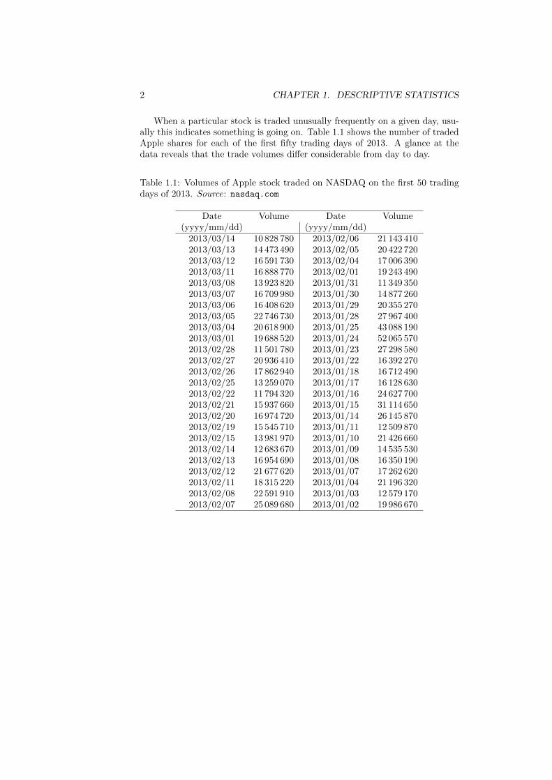
When a particular stock is traded unusually frequently on a given day, usu-ally this indicates something is going on. Table 1.1 shows the number of tradedApple shares for each of the first fifty trading days of 2013. A glance at thedata reveals that the trade volumes differ considerable from day to day.
Table 1.1: Volumes of Apple stock traded on NASDAQ on the first 50 tradingdays of 2013. Source: nasdaq.com
Date Volume Date Volume(yyyy/mm/dd) (yyyy/mm/dd)
2013/03/14 10 828 780 2013/02/06 21 143 4102013/03/13 14 473 490 2013/02/05 20 422 7202013/03/12 16 591 730 2013/02/04 17 006 3902013/03/11 16 888 770 2013/02/01 19 243 4902013/03/08 13 923 820 2013/01/31 11 349 3502013/03/07 16 709 980 2013/01/30 14 877 2602013/03/06 16 408 620 2013/01/29 20 355 2702013/03/05 22 746 730 2013/01/28 27 967 4002013/03/04 20 618 900 2013/01/25 43 088 1902013/03/01 19 688 520 2013/01/24 52 065 5702013/02/28 11 501 780 2013/01/23 27 298 5802013/02/27 20 936 410 2013/01/22 16 392 2702013/02/26 17 862 940 2013/01/18 16 712 4902013/02/25 13 259 070 2013/01/17 16 128 6302013/02/22 11 794 320 2013/01/16 24 627 7002013/02/21 15 937 660 2013/01/15 31 114 6502013/02/20 16 974 720 2013/01/14 26 145 8702013/02/19 15 545 710 2013/01/11 12 509 8702013/02/15 13 981 970 2013/01/10 21 426 6602013/02/14 12 683 670 2013/01/09 14 535 5302013/02/13 16 954 690 2013/01/08 16 350 1902013/02/12 21 677 620 2013/01/07 17 262 6202013/02/11 18 315 220 2013/01/04 21 196 3202013/02/08 22 591 910 2013/01/03 12 579 1702013/02/07 25 089 680 2013/01/02 19 986 670
1.2. SUMMARIZING DATA BY A FREQUENCY TABLE 3
How can we get a better idea of the typical daily volumes and the spreadaround the typical volumes? A good start is to rank the values from low tohigh:
10 828 780 , 11 349 350 , 11 501 780 , 11 794 320 , 12 509 870 ,12 579 170 , 12 683 670 , 13 259 070 , 13 923 820 , 13 981 970 ,14 473 490 , 14 535 530 , 14 877 260 , 15 545 710 , 15 937 660 ,16 128 630 , 16 350 190 , 16 392 270 , 16 408 620 , 16 591 730 ,16 709 980 , 16 712 490 , 16 888 770 , 16 954 690 , 16 974 720 ,17 006 390 , 17 262 620 , 17 862 940 , 18 315 220 , 19 243 490 ,19 688 520 , 19 986 670 , 20 355 270 , 20 422 720 , 20 618 900 ,20 936 410 , 21 143 410 , 21 196 320 , 21 426 660 , 21 677 620 ,22 591 910 , 22 746 730 , 24 627 700 , 25 089 680 , 26 145 870 ,27 298 580 , 27 967 400 , 31 114 650 , 43 088 190 , 52 065 570
(In R Commander, type the sort() function in the script window. The nameof the variable should be between the brackets.)
The values vary from 10.8 to 52.1 million shares per day. The middle valuein the ordered list is called the median. Because we have an even number ofvalues (50), there are two middle values: the values at position 25 (16 974 720)and 26 (17 006 390). In that case, the convention is to take the average of thetwo middle values as the median:
median =16 974 720 + 17 006 390
2= 16 990 555
The median gives an idea of the central tendency of the data distribution: halfof the days the value (the volume of traded shares) was less than the median,and the other half the value was more than the median.
We can summarize the ordered list in a frequency table. First, define classintervals that don’t overlap and cover all data. You don’t want too few classintervals (because that would leave out too much information), nor too many(because that wouldn’t summarize the information from the data). You alsowant the class intervals to have boundaries that are easy, rounded numbers.The class intervals don’t have to be of the same width. Let us define the firstclass interval as 10 000 000 to 15 000 000 (10 000 000 included, 15 000 000 notincluded), the second as 15 000 000 to 20 000 000, and so on, until 50 000 000to 55 000 000. A frequency table has three columns: class interval, absolutefrequency, and relative frequency (table 1.2). The absolute frequency (orcount) is how many values fall in each class interval. The first class interval(10 000 000 to 15 000 000) contains 13 values (verify!): the absolute frequencyfor this interval is 13. Find the absolute frequencies for the other class intervals.The relative frequency expresses the number of values in a class interval (theabsolute frequency) as a percentage of the total number of values in the dataset. For the first class interval (10 000 000 to 15 000 000) the relative frequencyis:
13
50× 100% = 26%
Verify the relative frequencies for the other class intervals. Show your work.The absolute frequencies add up to the number of values in the data set,
and the relative frequencies (before rounding) add up to 100%. If that is notthe case, you made a mistake.
4 CHAPTER 1. DESCRIPTIVE STATISTICS
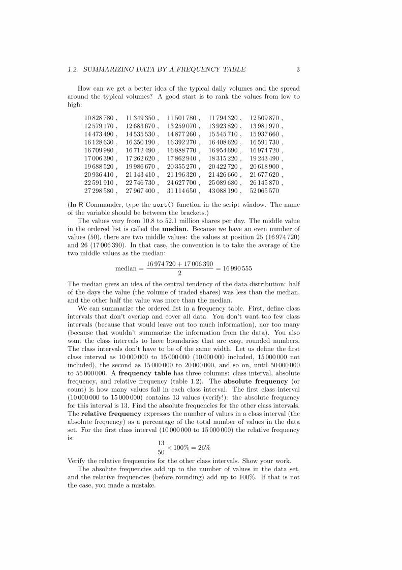
Table 1.2: Frequency table of the volumes of Apple stock traded on NASDAQon the first 50 trading days of 2013. Note. Class intervals include left boundariesand don’t include right boundaries.
Volume Absolute Relative(shares per day) frequency frequency (%)10 to 15 million 13 2615 to 20 million 19 3820 to 25 million 11 2225 to 30 million 4 830 to 35 million 1 235 to 40 million 0 040 to 45 million 1 245 to 50 million 0 050 to 55 million 1 2Sum: 50 100
1.3 Summarizing data by a density histogram
The frequency table gives you a pretty good idea of what the most commonvalues are, and how the values differ. One way to graph the information from afrequency table is to plot the values of the variable (in this case: the daily vol-umes) on the vertical axis, and the absolute or relative frequency on the verticalaxis. The heights of the bars represent the absolute or relative frequencies. Theareas of the bars don’t have a meaning. Such a bar chart is called a frequencyhistogram.
For reasons that will soon be clear, it is more interesting to plot a frequencytable in a bar chart where the areas of the bars represent the relative frequencies.Such a bar chart is called a density histogram. The height of each bar in adensity histogram represents the density of the data in the class interval.
To construct a density histogram, we have to find the height for each bar.How do we compute the height? Remember that the area of a rectangle (suchas the bars in the density histogram) is given by width times height:
area = width× height
The area of the bar is the relative frequency, the width of the bar is the widthof the class interval, and the height of the bar is the density. Hence:
relative frequency = width of the interval× density
Divide both sides by the width of the interval, to obtain:
density =relative frequency (%)
width of the interval
This formula is on the formula sheet. For the class interval from 10 million to15 million shares the relative frequency was 26% (table 1.2). Hence the densityfor this interval is:
density =26%
15 million shares− 10 million shares
1.3. SUMMARIZING DATA BY A DENSITY HISTOGRAM 5
=26%
5 million shares= 5.2%/million shares
Now that you know the height of the bar over the interval from 10 to 15 millionshares (5.2% per million shares), you can draw the bar. The density for theinterval from 10 to 15 million shares tells us which percentage of all 50 valuesfalls in each interval of one unit wide on the horizontal axis, assuming that thevalues in interval from 10 to 15 million shares would be uniformly distributed. Inthe interval from 10 to 15 million shares, about 5.2% of all values falls between10 and 11 million shares, about 5.2% of all values falls between 11 and 12 millionshares, about 5.2% of all values falls between 12 and 13 million shares, about5.2% of all values falls between 13 and 14 million shares, and about 5.2% of allvalues falls between 14 and 15 million shares. It is as if the bar is sliced upin vertical strips of one horizontal unit (here: one million shares) wide. Thedensity measures which percentage of all values falls in such a strip of one unitwide. Note the unit of measurement of density: percent per million shares.More generally, density is expressed in percent per unit on the horizontalaxis.
Given a data set such as table 1.1, you should be able to construct a frequencytable and a density histogram. The first assignment asks you to do exactly that.
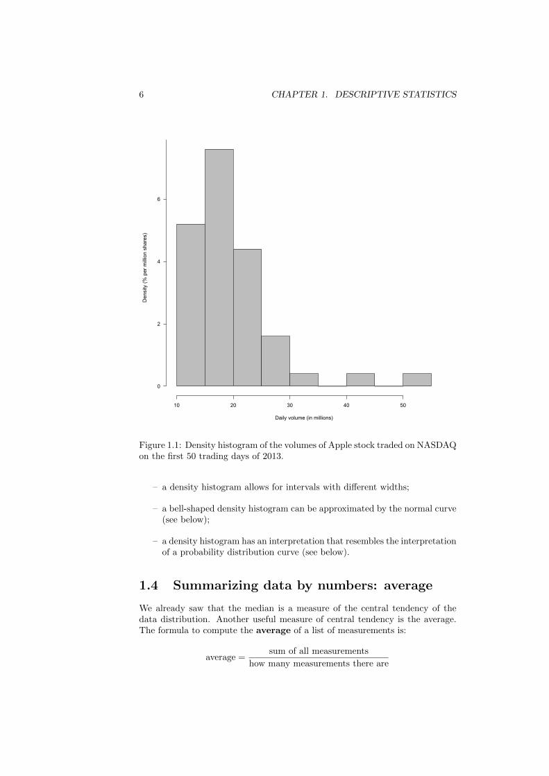
Figure 1.1 shows the density histogram as generated by R. A script to drawthis density histogram in R Commander is posted on the course web page.
Suppose you don’t have the data set or the frequency table, but just thedensity histogram (figure 1.1). On which percentage of trading days was thevolume of traded Apple shares between 20 and 30 million? Show in the densityhistogram what represents your answer. On (approximately) which percentageof trading days was the volume of traded Apple shares between 24 and 27million? Show in the density histogram what represents your answer.
We conclude that the area under de histogram between two values representsthe percentage of observations that falls between those two values.
What is the area under all of the histogram? %.
In a density histogram the vertical axis shows the density of the data. Theareas of the bars represent percentages. The area under a density histogramover an interval is the percentage of data that fall in that interval. The totalarea under a density histogram is 100%. (Freedman et al., 2007, p. 41)
A density histogram reveals the shape of the data distribution. To assessthe shape of the density histogram, locate the median on the horizontal axisand draw a vertical line. Is the histogram symmetric about the median, or is itskewed? Is the histogram skewed to the left (that is, with a long tail to the left)or to the right (with a long tail to the right)? Is the histogram bell-shaped?Watch this two-minute video clip (Rosling, 2015) that uses a histogram to showhow the world income distribution has changed over the last two centuries:
https://youtu.be/_JhD37gSNVU
Although a density histogram is somewhat more complicated than a fre-quency histogram, a density histogram has several advantages:
6 CHAPTER 1. DESCRIPTIVE STATISTICS
Daily volume (in millions)
Den
sity
(% p
er m
illio
n sh
ares
)
10 20 30 40 50
0
2
4
6
Figure 1.1: Density histogram of the volumes of Apple stock traded on NASDAQon the first 50 trading days of 2013.
– a density histogram allows for intervals with different widths;
– a bell-shaped density histogram can be approximated by the normal curve(see below);
– a density histogram has an interpretation that resembles the interpretationof a probability distribution curve (see below).
1.4 Summarizing data by numbers: average
We already saw that the median is a measure of the central tendency of thedata distribution. Another useful measure of central tendency is the average.The formula to compute the average of a list of measurements is:
average =sum of all measurements
how many measurements there are
1.5. SUMMARIZING DATA BY NUMBERS: STANDARD DEVIATION 7
Here is an example. Suppose you collected the price of the same bottle ofwine in five restaurants:
€ 2,€ 2,€ 4,€ 5,€ 7
The average price is:
average =€ 2 +€ 2 +€ 4 +€ 5 +€ 7
5=€ 20
5= € 4
A disadvantage is that the average is sensitive to outliers (exceptionally lowor exceptionally high values). Suppose that the list looked like this:
€ 2,€ 2,€ 4,€ 5,€ 22
The average of this list is:
average =€ 2 +€ 2 +€ 4 +€ 5 +€ 22
5=€ 35
5= € 7
The one exceptionally expensive bottle of € 22 pulled the average up quite a lot.In cases like this we often prefer to use a different measure of central tendency:the median. To find the median, first rank the values from low to high. Thentake the middle value. The median of the list {€ 2, € 2, € 4, € 5, € 22} is € 4.The median of the first list { € 2, € 2, € 4, € 5, € 7} is also € 4. As you cansee, the outlier doesn’t affect the median. When a density histogram is skewedor when there are outliers, the median usually is a better measure of the centraltendency. One example is the distribution of families by income (Freedmanet al., 2007, figure 4 p. 36).
1.5 Summarizing data by numbers: standarddeviation
We have seen how to summarize the central tendency of a data set. Anotherfeature we would like capture is the spread (or dispersion) of the data. Oneway to measure the spread is to look at how much the measurements deviatefrom the average. Let’s go back to the prices of the same bottle of wine in fiverestaurants:
€ 2,€ 2,€ 4,€ 5,€ 7
The average price is:
average =€ 2 +€ 2 +€ 4 +€ 5 +€ 7
5=€ 20
5= € 4
The deviation from the average measures how much a measurement is below(−) or above (+) the average:
deviation = measurement− average
The deviations are:
€ 2−€ 4 = −€ 2
€ 2−€ 4 = −€ 2
€ 4−€ 4 = € 0
€ 5−€ 4 = +€ 1
€ 7−€ 4 = +€ 3
8 CHAPTER 1. DESCRIPTIVE STATISTICS
To get an idea of the typical deviation, we could take the arithmetic mean ofthe deviations:
(−€ 2) + (−€ 2) +€ 0 + (+€ 1) + (+€ 3)
5= € 0
It can be easily proven that—whatever the list of measurements—the arithmeticmean of the deviations is always equal to 0: the negative deviations exactly can-cel out the positive ones. Therefore statisticians use the quadratic mean of thedeviations as a measure of the spread; the outcome is called the standard de-viation.
The standard deviation (SD) is a measure of the typical deviation of themeasurements from their mean. It is computed as the quadratic mean (or root-mean-square size) of the deviations from the average.
The quadratic mean is usually referred to as the root-mean-square (R-M-S)size. To obtain the standard deviation, find the deviations. The compute thequadratic mean (or root-mean-square size) of the deviations, apply the root-mean-square recipe in reverse order: first square the deviations, then find the(arithmetic) mean of the result, and finally take the (square) root. In ourexample:
1. Square the deviations:
(−€ 2)2 = €24
(−€ 2)2 = €24
(€ 0)2 = €20
(+€ 1)2 = €21
(+€ 3)2 = €29
By squaring we get rid of the minus signs. Note that the unit of measure-ment (here: €) is squared, too.
2. Next find the arithmetic mean (or average) of the results from the previousstep:
mean =€
24 +€ 24 +€ 20 +€ 21 +€ 29
5=€
218
5= € 23.6
The unit (€) is still squared (€ 2).
3. Finally take the square root of the result from the previous step:√€
23.6 ≈ € 1.90
This is the standard deviation. Note that by taking the square root, theunits are € again: the standard deviation has the same unit as themeasurements. In this case, the measurements were in euros, so thestandard deviation is also in euros.
1.5. SUMMARIZING DATA BY NUMBERS: STANDARD DEVIATION 9
Expressed as a formula, we get:
SD =
√sum of (deviations)
2
number of measurements
(The formula is on the formula sheet, so you don’t have to learn it by heart.)The formula above is for the standard deviation of a population. For reasons
I won’t explain, a better formula for the standard deviation of a sample is:
SD+ =
√sum of (deviations)
2
sample size×
√sample size
sample size− 1
that is, you compute the SD with the usual formula (the quadratic mean of thedeviations), which is the first factor in the equation above, and then multiplyby √
sample size
sample size− 1
(you don’t have to memorize this formula). Because the second factor is largerthan 1, the formula gives a value larger than SD. That’s why Freedman et al.(2007) use the notation SD+. For large samples, the difference between SD andSD+ is small. In what follows, we’ll use the SD formula for both samples andpopulations, unless stated explicitly otherwise. We’ll return to SD+ when wediscuss small samples.
Remember the following rule: few measurements are more than threeSDs from the average.1 This rule holds for histograms of any shape.
Measurements that are more than three SDs from the average (exceptionallysmall or exceptionally large measurements) are called outliers. To identifyoutliers, compute the standard scores of all measurements. The standard scoreexpresses how many standard deviations a measurement is below (−) or above(−) the average:
standard score =measurement− average
standard deviation
Converting measurements to standard scores is called standardizing.Let us return to the daily traded volumes of Apple shares (table 1.1). The
volumes of Apple shares trade on the first 50 trading days of 2013 have anaverage of 19 315 460 and a standard deviation of 7 466 246. On 14 March 2013only 10 828 780 Apple shares were traded. Is that volume exceptionally small?Compute the standard score for 10 828 780:
10 828 780− 19 315 460
7 466 246=−32 750 110
7 466 246≈ −1.13
De standard score of −1.13 means that the volume of 10 828 780 shares was1.13 standard deviations below the average. Because the absolute value of the
1A more precise statement can be made. It can be proven (Chebychev’s Theorem) that atleast 8/9 of the measurements fall within 3 SDs of the average, that is, between
[average− 3 · SD, average + 3 · SD]
Hence at most 1/9 of the measurements fall outside that interval. You don’t have to memorizethis.
10 CHAPTER 1. DESCRIPTIVE STATISTICS
standard score (after omitting the minus sign: 1.13) is smaller than 3, we don’tconsider 10 828 780 as an outlier.
Standard scores have no units. The following example illustrates this. Alist of incomes per person for most countries in the world (the Penn WorldTable, Heston et al. (2012)) has an average of $ 15 115 and a standard deviationof $ 18 651. Income per person in Belgium is $ 39 759. De standard score forincome per person in Belgium is:
$39 759− $15 115
$18 651=
$24 644
$18 651≈ 1.32
The units in the numerator ($) and denominator ($) cancel each other out, andhence the standard score has no units. That’s why Freedman et al. (2007) referto computing standard scores as converting a measurement to standard units.The standard score of 1.32 means that income per person in Belgium is 1.32standard deviations above the average of all countries in the list. So is incomeper person in Belgium an outlier?
Shortcut formula for the SD of 0-1 lists. Computing the SD is tedious.To estimate percentages, we’ll be dealing with lists that consist of just zeroesand ones (0-1 lists): for instance, we will model an employee with a privatepension plan as a 1, and an employee without a private pension plan as a 0.The following shortcut formula simplifies the calculation of the SD of 0-1lists: the standard deviation of a list that consist of just zeroes and ones can becomputed as:
SD of 0-1 list =
√(fraction of
ones in the list
)×(
fraction ofzeroes in the list
)(This formula is on the formula sheet, so no need to memorize. Just for your
information, I posted a proof on the course home page.)Here is an example. Consider the list {0, 1, 1, 1, 0}. The average is 3/5. The
deviations from the average are: {−3/5, 2/5, 2/5, 2/5,−3/5}, or {−0.6, 0.4, 0.4, 0.4,−0.6}.The SD is the root-mean-square size of the deviations:
1. Square the deviations: {0.36, 0.16, 0.16, 0.16, 0.36}
2. Next find the average of the squared deviations:
0.36 + 0.16 + 0.16 + 0.16 + 0.36
5=
1.20
5= 0.24
3. Finally take the square root to obtain the SD:
SD =√
0.24 ≈ 0.4898979
According to the shortcut rule we can compute the SD as:√(fraction of
ones
)×(
fraction ofzeroes
)which yields: √
3
5× 2
5=
√6
25=√
0.24 ≈ 0.4898979
which indeed yields the same result, with far fewer calculations.
1.6. THE NORMAL CURVE 11
1.6 The normal curve
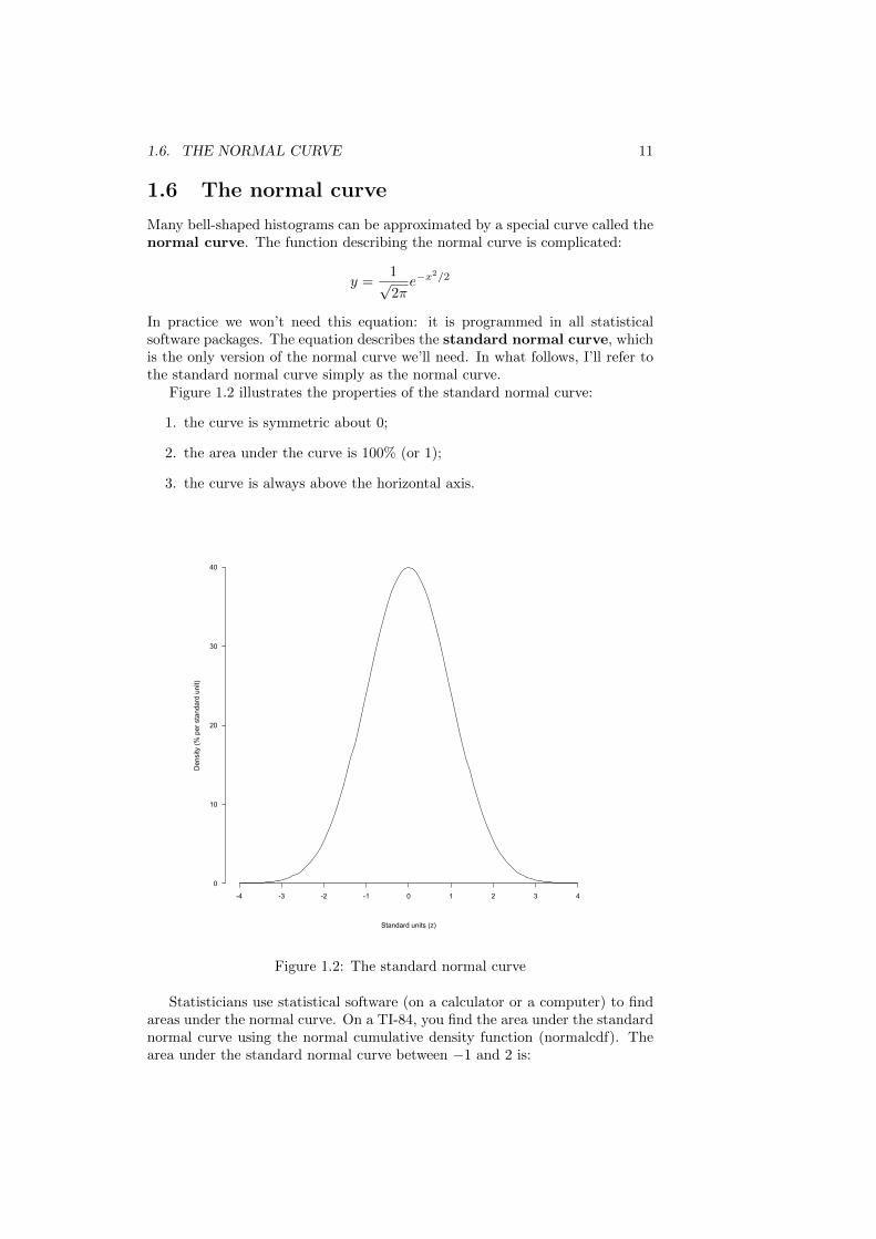
Many bell-shaped histograms can be approximated by a special curve called thenormal curve. The function describing the normal curve is complicated:
y =1√2πe−x2/2
In practice we won’t need this equation: it is programmed in all statisticalsoftware packages. The equation describes the standard normal curve, whichis the only version of the normal curve we’ll need. In what follows, I’ll refer tothe standard normal curve simply as the normal curve.
Figure 1.2 illustrates the properties of the standard normal curve:
1. the curve is symmetric about 0;
2. the area under the curve is 100% (or 1);
3. the curve is always above the horizontal axis.
0
10
20
30
40
Standard units (z)
Den
sity
(% p
er s
tand
ard
unit)
-4 -3 -2 -1 0 1 2 3 4
Figure 1.2: The standard normal curve
Statisticians use statistical software (on a calculator or a computer) to findareas under the normal curve. On a TI-84, you find the area under the standardnormal curve using the normal cumulative density function (normalcdf). Thearea under the standard normal curve between −1 and 2 is:
12 CHAPTER 1. DESCRIPTIVE STATISTICS
DISTR → normalcdf(−1,2)which yields approximately 0.8186. To express the area as a percentage, multiplyby 100%:
0.8186× 100% = 81.86%
The area under the standard normal curve to the right of −1 (that is, between−1 and infinity) is:
DISTR → normalcdf(−1,1099)The area under the standard normal curve to the left of 2 (that is, betweenminus infinity and 2) is:
DISTR → normalcdf(−1099, 2)For the exams, you have to use the TI-84 to find areas under the normal curve.On the course web page I posted an R script (area-under-normal-curve.R)that computes and plots the area under the normal curve between any twovalues on the horizontal axis. R Commander has a built-in function to find thearea under the normal curve in the left tail or in the right tail:
Distributions → Continuous distributions → Normal distribution→ Normal probabilities . . .
1.7 Approximating a density histogram by thenormal curve
These are scores of 100 job applicants who took a selection test:
74, 82, 70, 84, 54, 60, 79, 62, 72, 66, 72, 79, 73, 73, 84, 59, 53, 65, 62, 81,76, 67, 72, 89, 70, 72, 71, 78, 98, 58, 68, 89, 70, 62, 71, 56, 68, 68, 76, 63,63, 71, 82, 63, 98, 76, 74, 71, 52, 80, 80, 66, 69, 67, 70, 81, 62, 63, 76, 57,89, 60, 87, 80, 75, 71, 87, 59, 69, 65, 66, 67, 62, 87, 58, 58, 60, 54, 74, 83,48, 77, 79, 60, 84, 86, 68, 64, 83, 65, 77, 79, 68, 75, 77, 72, 47, 77, 68, 67
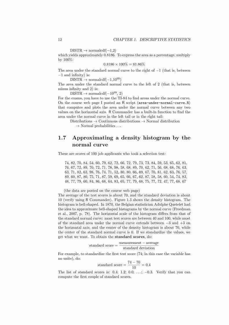
(the data are posted on the course web page)The average of the test scores is about 70, and the standard deviation is about10 (verify using R Commander). Figure 1.3 shows the density histogram. Thehistogram is bell-shaped. In 1870, the Belgian statistician Adolphe Quetelet hadthe idea to approximate bell-shaped histograms by the normal curve (Freedmanet al., 2007, p. 78). The horizontal scale of the histogram differs from that ofthe standard normal curve: most test scores are between 40 and 100, while mostof the standard area under the normal curve extends between −3 and +3 onthe horizontal axis; and the center of the density histogram is about 70, whilethe center of the standard normal curve is 0. If we standardize the values, weget what we want. To obtain the standard scores, do:
standard score =measurement− average
standard deviation
For example, to standardize the first test score (74; in this case the variable hasno units), do:
standard score =74− 70
10= 0.4
The list of standard scores is: 0.4; 1.2; 0.0; . . . ; −0.3. Verify that you cancompute the first couple of standard scores.
1.7. APPROXIMATING ADENSITY HISTOGRAMBYTHE NORMAL CURVE13
Test score (points)
Den
sity
(% p
er p
oint
)
40 50 60 70 80 90 100
0
1
2
3
Figure 1.3: Density histogram of 100 test scores
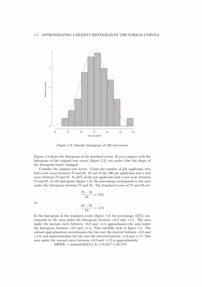
Figure 1.4 shows the histogram of the standard scores. If you compare with thehistogram of the original test scores (figure 1.3) you notice that the shape ofthe histogram hasn’t changed.
Consider the original test scores. Count the number of job applicants whohad a test score between 75 and 85: 25 out of the 100 job applicants had a testscore between 75 and 85. So 25% of the job applicants had a test score between75 and 85. In the histogram (figure 1.3), the percentage corresponds to the areaunder the histogram between 75 and 85. The standard scores of 75 and 85 are:
75− 70
10= +0.5
en85− 70
10= +1.5
In the histogram of the standard scores (figure 1.4) the percentage (25%) cor-responds to the area under the histogram between +0.5 and +1.5. The areaunder the normal curve between +0.5 and +1.5 approximates the area underthe histogram between +0.5 and +1.5. Now carefully look at figure 1.4. Thenormal approximation overestimates the bar over the interval between +0.5 and+1.0, and underestimates the bar over the interval between +1.0 and +1.5. Thearea under the normal curve between +0.5 and +1.5 is approximately:
DISTR → normalcdf(0.5,1.5) ≈ 0.2417 ≈ 24.17%
14 CHAPTER 1. DESCRIPTIVE STATISTICS
Standard units
Den
sity
(% p
er s
tand
ard
unit)
-3 -2 -1 0 1 2 3
0
10
20
30
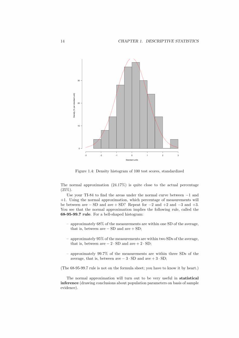
Figure 1.4: Density histogram of 100 test scores, standardized
The normal approximation (24.17%) is quite close to the actual percentage(25%).
Use your TI-84 to find the areas under the normal curve between −1 and+1. Using the normal approximation, which percentage of measurements willbe between ave − SD and ave + SD? Repeat for −2 and +2 and −3 and +3.You see that the normal approximation implies the following rule, called the68-95-99.7 rule. For a bell-shaped histogram:
– approximately 68% of the measurements are within one SD of the average,that is, between ave− SD and ave + SD;
– approximately 95% of the measurements are within two SDs of the average,that is, between ave− 2 · SD and ave + 2 · SD;
– approximately 99.7% of the measurements are within three SDs of theaverage, that is, between ave− 3 · SD and ave + 3 · SD;
(The 68-95-99.7 rule is not on the formula sheet; you have to know it by heart.)
The normal approximation will turn out to be very useful in statisticalinference (drawing conclusions about population parameters on basis of sampleevidence).
1.8. QUESTIONS FOR REVIEW 15
1.8 Questions for Review
1. What is the difference between a qualitative and a quantitative variable?Illustrate using examples where you consider different characteristics ofthe students in the class.
2. What is the difference between a parameter and a statistic?
3. What does descriptive statistics do?
4. What does statistical inference do?
5. How can you summarize the distribution of a numerical data set in a table?In a graph?
6. In a density histogram, what does the density represent? What are theunits of density? Explain for a hypothetical distribution of heights (incentimeter) of people.
7. When would the median be a better measure of the central tendency of adistribution than the mean? Illustrate by giving an example.
8. What does the standard deviation measure? How is the standard deviationcomputed?
9. What are the properties of the normal curve?
10. What does the standard score measure? How is the standard score com-puted?
11. What does the 68-95-99.7% rule say?
1.9 Exercises
1. Download the data file AAPL-HistoricalQuotes.csv from the course website:
http://homepages.vub.ac.be/~lmahens/STA201.html
and save the data file to your STA201 folder (directory). The data set containsdata about Apple stock. Run R Commander and load the data set: Data →Import data → from textfile, clipboard, or URL. . . . A window opens. For“Location of Data File” select Local file system.” For “Field Separator” select“Commas.” For “Decimal-Point Character” select “Period [.]”. Press OK, nav-igate to the data file AAPL-HistoricalQuotes.csv, abd double-click the file.Your data should now be loaded by R Commander. In the R Commander menu,click the View Data Set button. A new window opens, showing the data set.The variable volume is the variable from table 1.1. Now enter the following lineof script in the R script window:
h <- hist(Dataset$volume/1000000,right=FALSE)
and press the Submit button. This command will compute the numbers neededto make a histogram and store then in an object called h. Next, type in the R
script window:
16 CHAPTER 1. DESCRIPTIVE STATISTICS
h$breaks
and press the Submit button. The output window will display the breaks be-tween the intervals, that is, the boundaries of the intervals used by R when itcomputes the frequency table. Next, type in the R script window:
h$counts
and press the Submit button. The output window will display the absolutefrequencies (counts) of each interval. Next, type in the R script window:
h$density
and press the Submit button. The output window will display the densities ofeach interval. The densities are expressed as decimal fractions per horizontalunit; to get densities expressed as percentages per horizontal unit you have tomultiply by 100%. Finally, type in the R script window:
h$counts/sum(h$counts)
and press the Submit button. The output window will display the relativefrequencies for each interval; to get relative frequencies expressed as percentagesyou have to multiply by 100%.
2. Use the relative frequencies from table 1.2 to compute the densities for theother intervals. Add a column to show the densities. Then draw the densityhistogram on scale on squared paper.
3. Figure 1.1 shows that the daily traded volumes of Apple shares have askewed distribution. The average daily volume is 19 315 460 shares. Find themedian. Show your work. How do mean and median compare? Is that whatyou expected from the shape of the histogram? Explain.
4. Find the standard deviation of {1, 1, 1, 1, 0} using two methods: the usualformula (root-mean-square size of the deviations) and the shortcut formula for0-1 lists. Do you get the same result?
5. The daily traded volumes of Apple shares (table 1.1) have an average of19 315 460 and a standard deviation of 7 466 246. Is 52 065 570 an outlier? And43 088 190? Show your work and explain.
6. Use the TI-84 to find the areas under the standard normal curve:
(a) to the right of 1.87
(b) to the left of −5.20
(c) between −1 and +1
(d) between −2 and +2
(e) between −3 and +3
Make for every case a sketch, with the relevant area shaded. Verify your answersusing the R script. We’ll get back to cases (c), (d), and (e) in a moment.
1.9. EXERCISES 17
7. For the 100 given test scores, find which percentage of job applicants scoredbetween 50 and 60. Then use the normal approximation. Is the normal approx-imation close?
8. For 164 adult Belgian men born in 1962 the average height is 175.7 cen-timeter and the SD is 8.2 centimeter (Garcia and Quintana-Domeque, 2007).Suppose that the histogram of the 164 heights follows the normal curve (heightsusually do). What is, approximately, the percentage of men in this group witha height of 170 centimeter or less? What is, approximately, the percentage ofmen in this group with a height of between 170 centimeter and 180 centimeter?
9. Of the volumes of Apple shares traded in the first 50 trading days of 2013(p. 1.2) the average is 19 315 460 and the SD is 7 466 246. Find the actualpercentage of values between:
ave− SD and ave + SD;
ave− 2 · SD and ave + 2 · SD;
ave− 3 · SD and ave + 3 · SD;
Does the 68-95-99.7 rule give a good approximation? Why (not)?

18 CHAPTER 1. DESCRIPTIVE STATISTICS
Chapter 2
Probability distributions
2.1 Chance experiments
Examples of chance experiments are: rolling a die and counting the dots;tossing a coin and observing whether you get heads or tails; or randomly drawinga card from a well-shuffled deck of cards and observing which card you get.
It is convenient to think of a chance experiment in terms of the followingchance model: randomly drawing one or more tickets from a box. For instance,rolling a die is modeled as randomly drawing a ticket from the box:
1 2 3 4 5 6
In R:
box <- c(1,2,3,4,5,6)
sample(box,1)
Tossing a coin is like randomly drawing a ticket from the box:
heads tails
In R:
box <- c("heads","tails")
sample(box,1)
2.2 Frequency interpretation of probability
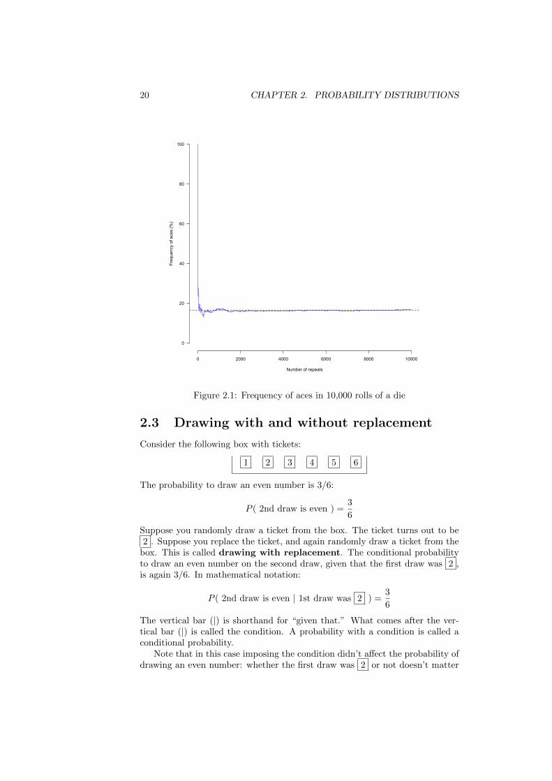
Consider the following chance experiment. Roll a die and count the dots. Ifyou get an ace (1), write down 1; if you don’t get an ace (2, 3, 4, 5, or 6),write down 0. Repeat the experiment many times. After each roll, computethe relative frequency of aces up to that point. Make a graph with the numberof tosses on the horizontal axis and the relative frequency on the vertical axis.Figure 2.1 shows the result of 10 000 repetitions in such an experiment. Thefrequency of aces tends towards 1/6 (16.666 . . .%, the horizontal dashed line).The frequency interpretation of probability states that the probability ofan event is the percentage to which the relative frequency tends if you repeat thechance experiment over and over, independently and under the same conditions(Freedman et al., 2007, p. 222).
19
20 CHAPTER 2. PROBABILITY DISTRIBUTIONS
0 2000 4000 6000 8000 10000
0
20
40
60
80
100
Number of repeats
Freq
uenc
y of
ace
s (%
)
Figure 2.1: Frequency of aces in 10,000 rolls of a die
2.3 Drawing with and without replacement
Consider the following box with tickets:
1 2 3 4 5 6
The probability to draw an even number is 3/6:
P ( 2nd draw is even ) =3
6
Suppose you randomly draw a ticket from the box. The ticket turns out to be2 . Suppose you replace the ticket, and again randomly draw a ticket from the
box. This is called drawing with replacement. The conditional probabilityto draw an even number on the second draw, given that the first draw was 2 ,is again 3/6. In mathematical notation:
P ( 2nd draw is even | 1st draw was 2 ) =3
6
The vertical bar (|) is shorthand for “given that.” What comes after the ver-tical bar (|) is called the condition. A probability with a condition is called aconditional probability.
Note that in this case imposing the condition didn’t affect the probability ofdrawing an even number: whether the first draw was 2 or not doesn’t matter
2.4. THE SUM OF DRAWS 21
for the second draw, because we replaced the ticket after the first draw. In bothcases, the probability of getting an even number was the same (3/6):
P ( 2nd draw is even | 1st draw was 2 ) = P ( 2nd draw is even )
The two events (getting an even number on the second draw, and getting an evennumber on the second draw) are said to be independent: the probability of thesecond event is not affected by how the first event turned out. That is becausewe were drawing with replacement. When drawing with replacement, theevents are independent.
Now consider a different chance experiment. Suppose you randomly draw aticket from the box. The ticket turns out to be 2 . Suppose you don’t replacethe ticket. The box now looks like this:
1 3 4 5 6
If we now again randomly draw a ticket from the box, this is called drawingwithout replacement. The conditional probability to draw an even numberon the second draw, given that the first draw was 2 now is :
P ( 2nd draw is even | 1st draw was 2 ) =2
5
In this case, what happened in the first draw (as expressed by the condition
“1st draw was 2 ”) does make a difference: the probability of getting an evennumber differs:
P ( 2nd draw is even | 1st draw was 2 ) 6= P ( 2nd draw is even )
The two events (getting an even number on the second draw, and getting an evennumber on the second draw) are said to be dependent: the probability of thesecond event is affected by how the first event turned out. That is because wewere drawing without replacement. When drawing without replacement,the events are dependent.
Think of a population as a box with tickets. A random sample is like drawinga number of tickets without replacement from this box. The number of draws isthe sample size. Remember this. We’ll use this box model when doing statisticalinference.
2.4 The sum of draws
For the theory of statistical inference, we’ll frequently use the concept of thesum of draws. Here’s a simple example: roll a die twice, and add the numbers.The chance model has the following box:
1 2 3 4 5 6
Draw two tickets with replacement from the box, and add the outcomes. Theresult is the sum of draws.
The sum of draws is a brief way to say the following (Freedman et al.,2007, p. 280):
22 CHAPTER 2. PROBABILITY DISTRIBUTIONS
– Draw tickets from a box.
– Add the numbers on the tickets.
As the following activity makes clear, the sum of draws is itself a random vari-able:
(a) Conduct the chance experiment above using an actual die or the followingR script:
box <- c(1,2,3,4,5,6)
sample(box,1) + sample(box,1)
(b) Repeat the experiment a couple of times and write up the outcomes (usingan actual die, or in R by running the line sample(box,1)+sample(box,1).Would it be fair to say that the sum of draws is a chance variable? Explain.
2.5 Picking an appropriate chance model
We model a population as a box with tickets. Taking a random sample is likerandomly drawing a number of tickets from the box, without replacement; thenumber of draws is the sample size. In order to use such a chance model forinference, we will use some interesting properties of the sum of draws. The trickis to set up the chance model in such a way that the chance variable of interestis the sum of draws, or is computed from the sum of draws. An example clarifiesmy argument.
Suppose you roll a die three times, and want to know what the sum ofthe outcomes is. What is the appropriate chance model? What is the chancevariable?An appropriate chance model is a box with six tickets:
1 2 3 4 5 6
and the chance variable is the sum of three random draws with replacementfrom the box. For instance, if you roll 3, 2, and 6, this corresponds to drawingtickets 3 , 2 , and 6 . The sum of draws ( 3 + 2 + 6 = 11) is obtained byadding up the outcomes.
Now suppose that we are interested in another question: how many times(out of three rolls) will we get a six? First, we need the appropriate chancemodel. When we roll a die, when can get two kinds of outcomes: either we geta six (we’ll label this outcome as a success), or we get another number (1, 2, 3,4, 5: not a success). The term success is used here in a technical meaning: theoutcome we are interested in. Note that we classify the outcomes of a singleroll as a success or not a success. In such a case, the appropriate chance modelis a box with six tickets: one ticket 1 for the outcome 6 labelled as a success,
and five tickets 0 for the outcomes 1, 2, 3, 4, or 5 labelled as not a success:
0 0 0 0 0 1
2.6. PROBABILITY DISTRIBUTIONS 23
Now we are interested in the number of sixes in three rolls, so we need to countthe sixes. Counting the sixes is the same thing as taking the sum of threedraws from the 0-1 box. For instance, if you roll 3, 2, and 6, this correspondsto drawing tickets 0 , 0 , and 1 (we classified each outcome as a success or
not a success). The sum of draws ( 0 + 0 + 1 = 1) is the number of sixes(the number of successes). A box like this, with tickets that can only takevalues 0 and 1, is called a 0-1 box. Remember that when the problem is one ofclassifying and counting, the appropriate box is a 0-1 box.
Here’s a real-world example. Suppose you are the marketing manager of atelecommunications company that doesn’t cover Brussels yet. You would like tofind out which percentage of households in Brussels already has a tablet. Thepopulation of interest is all households in Brussels. Think of each householdin Brussels as a ticket in a box, so there are as many tickets as households. Aticket takes value 1 if the household has a tablet, and 0 if the household doesn’t.Taking a random sample of households is like randomly drawing tickets withoutreplacement from this 0-1 box. The number of households in the sample whohave a tablet is the sum of draws. The percentage of households in the samplewho have a tablet is:
sample percentage =sum of draws
size of the sample× 100%
2.6 Probability distributions
Chance experiments can be described using probability distributions. In whatfollows, we’ll focus on the probability distribution of the sum of draws. Supposeyou roll a die twice and add the outcomes. The chance model is: randomlydraw two tickets with replacement from the box
1 2 3 4 5 6
and add the outcomes.The chance variable (the sum of the two draws) can take the following val-
ues: {2, 3, 4, 5, 6, 7, 8, 9, 10, 11, 12} (the chance variable is discrete; we won’tdevelop the theory for continuous chance variables). For each of these possibleoutcomes, we can compute the probability. There are 36 possible combinations:
1 2 3 4 5 61 2 3 4 5 6 72 3 4 5 6 7 83 4 5 6 7 8 94 5 6 7 8 9 105 6 7 8 9 10 116 7 8 9 10 11 12
Each of these 36 combinations has the same probability, and as the probabilitieshave to add up to 1, each combination has a probability of 1/36. By applyingthe rules or probability, we can find the probability that the sum of draws takesthe value 2, and then repeat the work to find the probability that the sum ofdraws takes the value 3, and so on. There are for instance two combinationsthat yield a sum of 3:
24 CHAPTER 2. PROBABILITY DISTRIBUTIONS
– when the first draw is 1 and the second draw is 2 (row 1, column 2 in thetable above)
– when the first draw is 2 and the second draw is 1 (row 2, column 1)
The probability that the sum of draws is 3 is therefore equal to:
P (sum is 3) = P [(first 1, than 2) or (first 2, then 1)]
Apply the addition rule (Freedman et al., 2007, pp. 241–242) to obtain:
P (sum is 3) = P (first 1, than 2) + P (first 2, then 1)− something
The third term (“minus something”) is equal to zero because the events (first 1,than 2) and (first 2, then 1) are mutually exclusive (two events are mutuallyexclusive when as one event happens, the other cannot happen at the sametime). So we get:
P (sum is 3) = P (first 1, than 2) + P (first 2, then 1)− 0 =1
36+
1
36=
2
36
If you do this for all other possible values of the chance variable, you get thefollowing table:
outcome 2 3 4 5 6 7 8 9 10 11 12probability 1
36236
336
436
536
636
536
436
336
236
136
A table that shows all possible values for a (discrete) chance variable and thecorresponding probabilities is called a probability distribution.
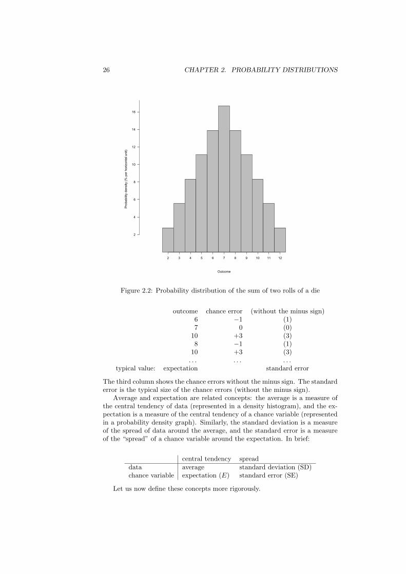
We can graph the probability distribution as a bar chart. On the horizontalaxis we put the chance variable, and we construct the bar chart in such a waythat the area of a bar shows the probability (expressed as a percentage), just asin a density histogram the area of a bar showed the relative frequency (expressedas a percentage) of the data over the interval. That is why Freedman et al. (2007,pp. 310–316) call such a bar chart a probability histogram. For a discrete chancevariable the convention is to center the bars on the values that the variable cantake: the bar over 2 will start at 1.5 and end at 2.5; the bar over 3 will startat 2.5 and end at 3.5, and so on. The width of each bar is equal to 1. Theheight of each bar in a probability distribution is called probability density:the probability per unit on the horizontal axis. We find the probability densitiesby applying the formula for the area of a rectangle:
area = width× height
We want the area to represent the probability (expressed as a percentage) andthe height to represent the probability density (expressed as percent per uniton the horizontal axis), and hence the equation becomes:
probability = width of interval on horizontal axis× probability density
Divide both sides of the equation by (width of interval on horizontal axis) toobtain:
probability density =probability
width of interval on horizontal axis
2.6. PROBABILITY DISTRIBUTIONS 25
Because the width of each interval on horizontal axis is one unit of the horizontalaxis, this becomes:
probability density = probability per unit on the horizontal axis
which gives us the meaning of probability density.
For example, the probability to get a 7 is 6/36 (= 16.66 . . .%). The proba-bility density over the interval from 6.5 to 7.5 then is equal to:
probability density =16.66 . . .%
7.5− 6.5= 16.66 . . .% per per unit on the horizontal axis
Figure 2.2 shows the corresponding bar chart representing the probabilitydistribution. The curve traced by the bar chart of the probability distributionis called the probability density function. The probability density functionhas the following properties:
– the curve is always on or above the horizontal axis, that is, the probabilitydensity (on the vertical axis) is always 0 or positive;
– de area under the curve is equal to 1 (or 100%);
– the area under the curve between two values on the horizontal axis givesthe probability.
The probability distribution has an expectation and a standard error. Thefollowing example illustrates the intuition of these concepts. Roll a die twiceand add the numbers. You can do that with an actual die, or run the followingR script:
box <- c(1,2,3,4,5,6)
sample(box,1) + sample(box,1)
Repeat this a couple of times, and write down the outcomes. You will getsomething like {6, 7, 10, 8, 10, . . . }. The outcomes are random. The lowestvalue you can get is 2 (when you roll two aces), and the highest value is 12(when you roll two sixes). If you repeat the experiment many times you’ll noticethat those extreme values occur only occasionally; values like 6, 7, or 8 occurmuch more frequently. The expectation is the typical value that the randomvariable will take; the value around which the outcomes vary. Another wayto think about the expectation is as the center of the probability distribution(figure 2.2). In this case the expectation is 7 (we’ll see below how to computethe expectation). Now define the difference between the outcome of a chanceexperiment and the expectation as the chance error. For instance, our firstoutcome was 6, the expectation is 7, and hence the chance error was:
chance error = outcome− expectation = 6− 7 = −1
(the negative value of 1 means that the outcome was 1 below the expectation).
If we compute the chance errors for the other outcomes, we get:
26 CHAPTER 2. PROBABILITY DISTRIBUTIONS
Outcome
Pro
babi
lity
dens
ity (%
per
hor
izon
tal u
nit)
2 3 4 5 6 7 8 9 10 11 12
2
4
6
8
10
12
14
16
Figure 2.2: Probability distribution of the sum of two rolls of a die
outcome chance error (without the minus sign)6 −1 (1)7 0 (0)
10 +3 (3)8 −1 (1)
10 +3 (3). . . . . . . . .
typical value: expectation standard error
The third column shows the chance errors without the minus sign. The standarderror is the typical size of the chance errors (without the minus sign).
Average and expectation are related concepts: the average is a measure ofthe central tendency of data (represented in a density histogram), and the ex-pectation is a measure of the central tendency of a chance variable (representedin a probability density graph). Similarly, the standard deviation is a measureof the spread of data around the average, and the standard error is a measureof the “spread” of a chance variable around the expectation. In brief:
central tendency spreaddata average standard deviation (SD)chance variable expectation (E) standard error (SE)
Let us now define these concepts more rigorously.

2.7. INTERMEZZO: A WEIGHTED AVERAGE 27
2.7 Intermezzo: a weighted average
To define the expectation and standard error of a discrete chance variable, weneed the concept of a weighted average. A weighted arithmetic average ofa list of numbers is obtained by multiplying each value in the list by a weightand adding up the outcomes; each of the weights is a number between zero(included) and one (included), and the weights add up to one. Suppose the firstvalue in the list is x1 and its weight is w1, the second value in the list is x2 andwith weight w2, . . . , and the last (nth) value in the list is xn and with weightwn, then the weighted average is:
(w1 × x1) + (w2 × x2) + . . .+ (wn × xn)
An example is the way a professor computes the students’ grades for a course.Here are the weights for the graded components of a course, and the results fora student:
component weight (%) result (score/20)assignment 1 7.50 12assignment 2 7.50 14assignment 3 7.50 16assignment 4 7.50 12participation and preparedness 10.00 16midterm exam 30.00 12final exam 30.00 17
Each weight is between 0 and 1: 7.50 percent is 0.075, 10 percent is 0.10, and30 percent is 0.30. Moreover, the sum of the weights is equal to 1:
7.50% + 7.50% + 7.50% + 7.50% + 10.00% + 30.00% + 30.00% = 100% = 1
The weighted average of the scores is:
(0.075× 12) + (0.075× 14) + (0.075× 16) + (0.075× 12)
+(0.10× 16) + (0.30× 12) + (0.30× 17) = 14.35
So this student has an overall score of 14.35/20.
2.8 Expectation (E)
Just as the average is a measure of the central tendency of a density histogram,the expectation of a chance variable is in a sense a measure for the centraltendency of a probability distribution. For a discrete chance variable, the ex-pectation is defined as the weighted average of all possible values that thechance variable can take; the weights are the probabilities.
The probability distribution of the sum of two rolls of a die is:
outcome 2 3 4 5 6 7 8 9 10 11 12probability 1
36236
336
436
536
636
536
436
336
236
136
The expectation of the chance variable “sum of two rolls of a die” (or of twodraws with replacement from a box with the tickets {1,2,3,4,5,6}) is the weighted
28 CHAPTER 2. PROBABILITY DISTRIBUTIONS
average:
2× 1
36+ 3× 2
36+ 4× 3
36+ 5× 4
36+ 6× 5
36+ 7× 6
36+ 8× 5
36
+9× 4
36+ 10× 3
36+ 11× 2
36+ 12× 1
36
=2 + 6 + 12 + 20 + 30 + 42 + 40 + 36 + 30 + 22 + 12
36=
252
36= 7
Let the operator E denote the expectation:
E(sum of two rolls of die) = 7
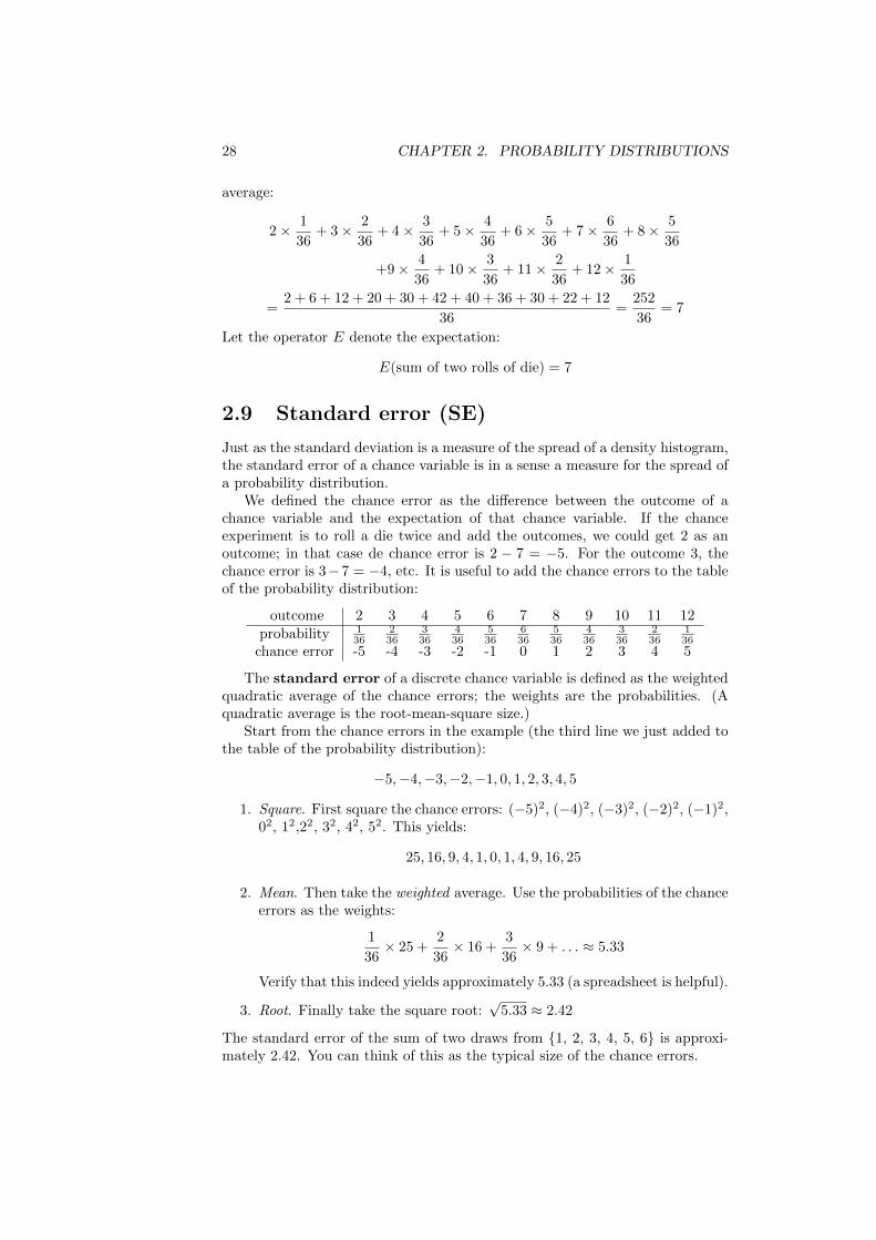
2.9 Standard error (SE)
Just as the standard deviation is a measure of the spread of a density histogram,the standard error of a chance variable is in a sense a measure for the spread ofa probability distribution.
We defined the chance error as the difference between the outcome of achance variable and the expectation of that chance variable. If the chanceexperiment is to roll a die twice and add the outcomes, we could get 2 as anoutcome; in that case de chance error is 2 − 7 = −5. For the outcome 3, thechance error is 3−7 = −4, etc. It is useful to add the chance errors to the tableof the probability distribution:
outcome 2 3 4 5 6 7 8 9 10 11 12probability 1
36236
336
436
536
636
536
436
336
236
136
chance error -5 -4 -3 -2 -1 0 1 2 3 4 5
The standard error of a discrete chance variable is defined as the weightedquadratic average of the chance errors; the weights are the probabilities. (Aquadratic average is the root-mean-square size.)
Start from the chance errors in the example (the third line we just added tothe table of the probability distribution):
−5,−4,−3,−2,−1, 0, 1, 2, 3, 4, 5
1. Square. First square the chance errors: (−5)2, (−4)2, (−3)2, (−2)2, (−1)2,02, 12,22, 32, 42, 52. This yields:
25, 16, 9, 4, 1, 0, 1, 4, 9, 16, 25
2. Mean. Then take the weighted average. Use the probabilities of the chanceerrors as the weights:
1
36× 25 +
2
36× 16 +
3
36× 9 + . . . ≈ 5.33
Verify that this indeed yields approximately 5.33 (a spreadsheet is helpful).
3. Root. Finally take the square root:√
5.33 ≈ 2.42
The standard error of the sum of two draws from {1, 2, 3, 4, 5, 6} is approxi-mately 2.42. You can think of this as the typical size of the chance errors.
2.10. EXPECTATION AND SE FOR THE SUM OF DRAWS 29
2.10 Expectation and SE for the sum of draws
When doing statistical inference, we’ll use the sum of draws with replacementfrom a box with tickets. The formulas for the expectation and the standarderror of discrete probability distributions from the previous sections also applyif the chance variable is a sum of draws. However, the computations can becometedious. It can be shown that the following formulas hold:
E(sum of draws) = (number of draws)× (average of box)
SE(sum of draws) =√
number of draws× (SD of the box)
“Average of box” means: the average of the values on the tickets in the box;similarly “SD of the box” means the SD of the values on the tickets in the box.You don’t have to memorize these formulas; they are on the formula sheet. Ininference, the box will represent the population, so the average of the box is thepopulation average and the SD of the box is the population SD.
Let us apply these formulas to the example from the previous sections: rolla die twice and add the outcomes. The chance model is: randomly draw twotickets with replacement from the box
1 2 3 4 5 6
and add the outcomes. We found in the previous sections that the expectationis 7 and the SE is approximately 2.42. What is we use the formulas for theexpectation and the SE of the sum of draws?
To apply the formula for the expectation of the sum of draws we first needthe average of the box:
average of box =1 + 2 + 3 + 4 + 5 + 6
6=
21
6
The expectation of the sum of two draws is:
E(sum of draws) = (number of draws)× (average of box) = 2× 21
6=
21
3= 7
This is the same number we found be applying the definition of the expectation.To apply the formula for the standard error for the sum of draws, we first
need the SD of the box; the SD of the box is about 1.71 (exercise: verify this).Then apply the formula for the standard error for the sum of draws:
SE (sum of draws) =√
number of draws× (SD of the box) ≈√
2× 1.71 ≈ 2.42
This is the same number we found be applying the definition of the standarderror.
2.11 The Central Limit Theorem
Consider again the chance experiment: roll a die twice and add the outcomes.The chance model is: randomly draw two tickets with replacement from the box
1 2 3 4 5 6
30 CHAPTER 2. PROBABILITY DISTRIBUTIONS
OutcomeD
ensi
ty (%
per
uni
t on
the
horiz
onta
l axi
s)
1 2 3 4 5 6
10
20
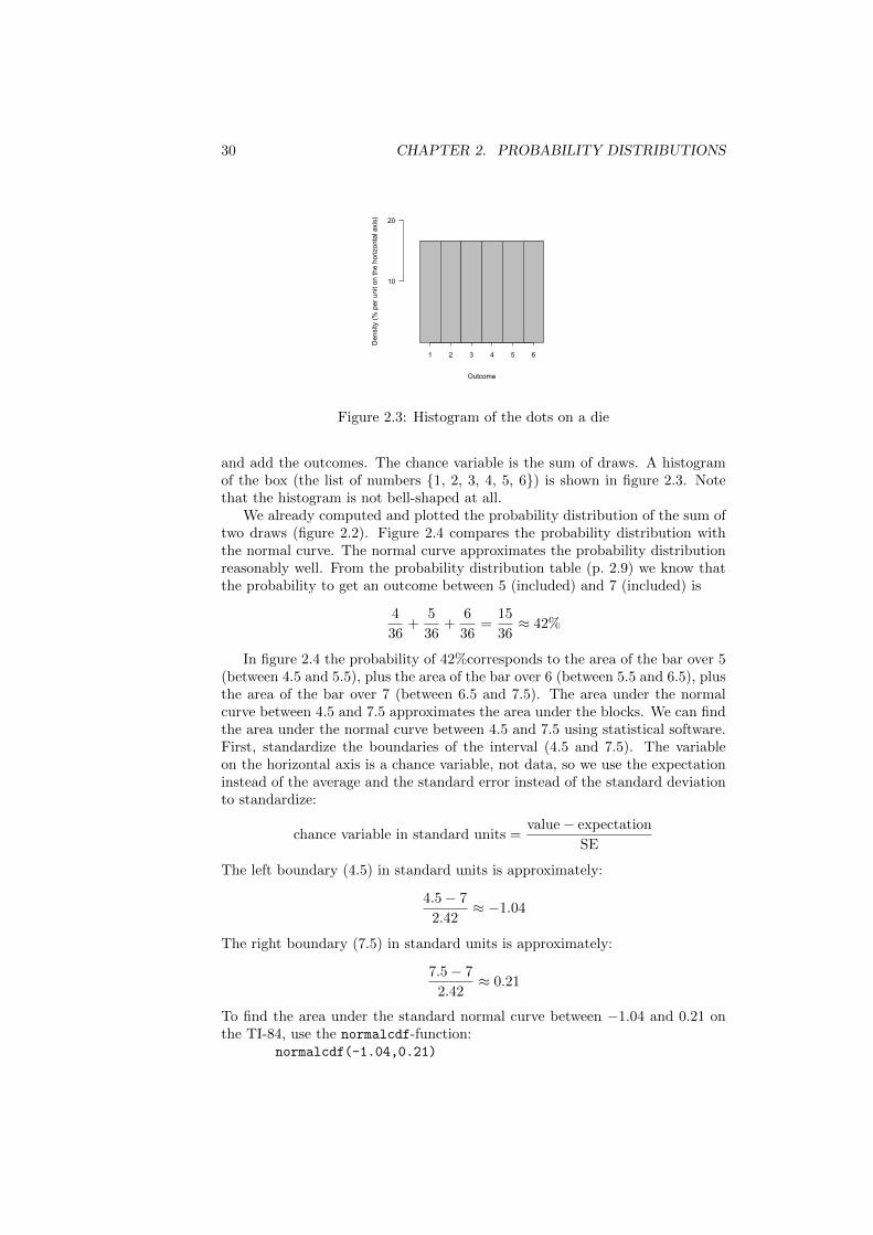
Figure 2.3: Histogram of the dots on a die
and add the outcomes. The chance variable is the sum of draws. A histogramof the box (the list of numbers {1, 2, 3, 4, 5, 6}) is shown in figure 2.3. Notethat the histogram is not bell-shaped at all.
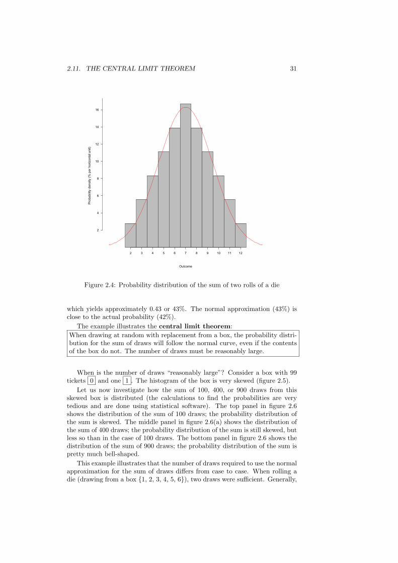
We already computed and plotted the probability distribution of the sum oftwo draws (figure 2.2). Figure 2.4 compares the probability distribution withthe normal curve. The normal curve approximates the probability distributionreasonably well. From the probability distribution table (p. 2.9) we know thatthe probability to get an outcome between 5 (included) and 7 (included) is
4
36+
5
36+
6
36=
15
36≈ 42%
In figure 2.4 the probability of 42%corresponds to the area of the bar over 5(between 4.5 and 5.5), plus the area of the bar over 6 (between 5.5 and 6.5), plusthe area of the bar over 7 (between 6.5 and 7.5). The area under the normalcurve between 4.5 and 7.5 approximates the area under the blocks. We can findthe area under the normal curve between 4.5 and 7.5 using statistical software.First, standardize the boundaries of the interval (4.5 and 7.5). The variableon the horizontal axis is a chance variable, not data, so we use the expectationinstead of the average and the standard error instead of the standard deviationto standardize:
chance variable in standard units =value− expectation
SE
The left boundary (4.5) in standard units is approximately:
4.5− 7
2.42≈ −1.04
The right boundary (7.5) in standard units is approximately:
7.5− 7
2.42≈ 0.21
To find the area under the standard normal curve between −1.04 and 0.21 onthe TI-84, use the normalcdf-function:
normalcdf(-1.04,0.21)
2.11. THE CENTRAL LIMIT THEOREM 31
Outcome
Pro
babi
lity
dens
ity (%
per
hor
izon
tal u
nit)
2 3 4 5 6 7 8 9 10 11 12
2
4
6
8
10
12
14
16
Figure 2.4: Probability distribution of the sum of two rolls of a die
which yields approximately 0.43 or 43%. The normal approximation (43%) isclose to the actual probability (42%).
The example illustrates the central limit theorem:
When drawing at random with replacement from a box, the probability distri-bution for the sum of draws will follow the normal curve, even if the contentsof the box do not. The number of draws must be reasonably large.
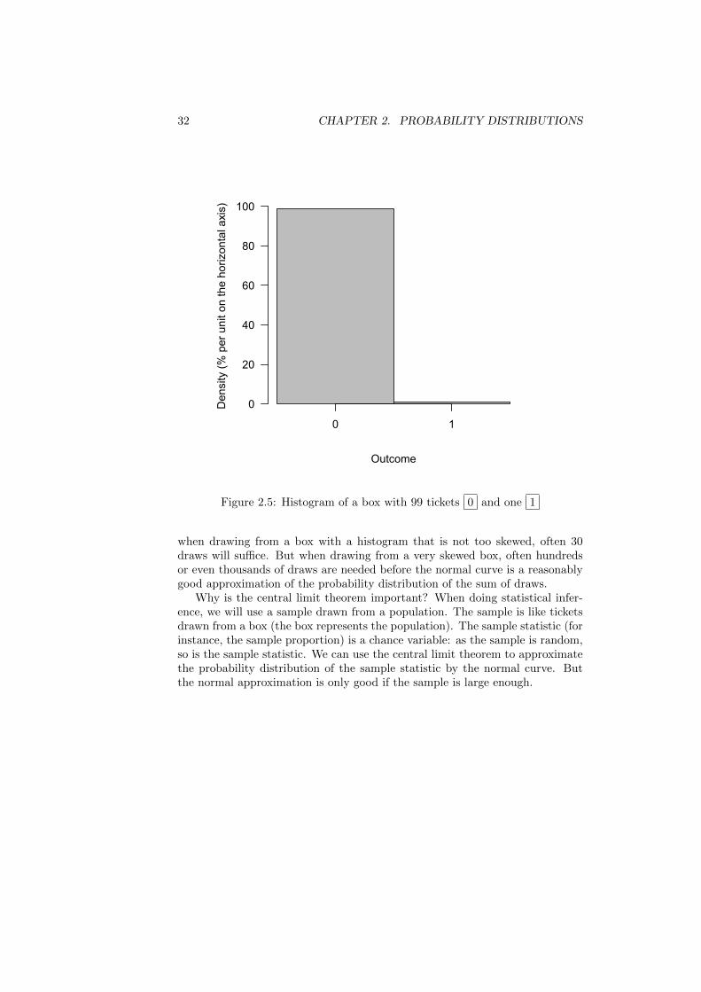
When is the number of draws “reasonably large”? Consider a box with 99tickets 0 and one 1 . The histogram of the box is very skewed (figure 2.5).
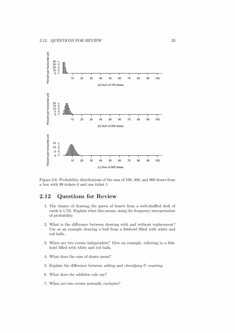
Let us now investigate how the sum of 100, 400, or 900 draws from thisskewed box is distributed (the calculations to find the probabilities are verytedious and are done using statistical software). The top panel in figure 2.6shows the distribution of the sum of 100 draws; the probability distribution ofthe sum is skewed. The middle panel in figure 2.6(a) shows the distribution ofthe sum of 400 draws; the probability distribution of the sum is still skewed, butless so than in the case of 100 draws. The bottom panel in figure 2.6 shows thedistribution of the sum of 900 draws; the probability distribution of the sum ispretty much bell-shaped.
This example illustrates that the number of draws required to use the normalapproximation for the sum of draws differs from case to case. When rolling adie (drawing from a box {1, 2, 3, 4, 5, 6}), two draws were sufficient. Generally,
32 CHAPTER 2. PROBABILITY DISTRIBUTIONS
Outcome
Den
sity
(% p
er u
nit o
n th
e ho
rizon
tal a
xis)
0 1
0
20
40
60
80
100
Figure 2.5: Histogram of a box with 99 tickets 0 and one 1
when drawing from a box with a histogram that is not too skewed, often 30draws will suffice. But when drawing from a very skewed box, often hundredsor even thousands of draws are needed before the normal curve is a reasonablygood approximation of the probability distribution of the sum of draws.
Why is the central limit theorem important? When doing statistical infer-ence, we will use a sample drawn from a population. The sample is like ticketsdrawn from a box (the box represents the population). The sample statistic (forinstance, the sample proportion) is a chance variable: as the sample is random,so is the sample statistic. We can use the central limit theorem to approximatethe probability distribution of the sample statistic by the normal curve. Butthe normal approximation is only good if the sample is large enough.
2.12. QUESTIONS FOR REVIEW 33
(a) Sum of 100 draws
Per
cent
per
hor
izon
tal u
nit
010203040
10 20 30 40 50 60 70 80 90 100
(b) Sum of 400 draws
Per
cent
per
hor
izon
tal u
nit
05101520
10 20 30 40 50 60 70 80 90 100
(c) Sum of 900 draws
Per
cent
per
hor
izon
tal u
nit
051015
10 20 30 40 50 60 70 80 90 100
Figure 2.6: Probability distributions of the sum of 100, 400, and 900 draws froma box with 99 tickets 0 and one ticket 1
2.12 Questions for Review
1. The chance of drawing the queen of hearts from a well-shuffled deck ofcards is 1/52. Explain what this means, using the frequency interpretationof probability.
2. What is the difference between drawing with and without replacement?Use as an example drawing a ball from a fishbowl filled with white andred balls.
3. When are two events independent? Give an example, referring to a fish-bowl filled with white and red balls.
4. What does the sum of draws mean?
5. Explain the difference between adding and classifying & counting.
6. What does the addition rule say?
7. When are two events mutually exclusive?
34 CHAPTER 2. PROBABILITY DISTRIBUTIONS
8. What is a probability distribution for a discrete chance variable? Whichproperties should it have?
9. What is a probability density histogram? Which properties does it have?
10. What is probability density?
11. What is a chance error?
12. What is a weighted average?
13. What is the expectation of a discrete chance variable?
14. What is the standard error of a discrete chance variable?
15. What does the Central Limit Theorem say?
2.13 Exercises
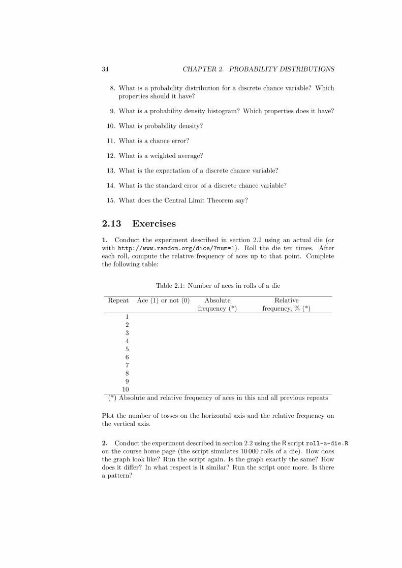
1. Conduct the experiment described in section 2.2 using an actual die (orwith http://www.random.org/dice/?num=1). Roll the die ten times. Aftereach roll, compute the relative frequency of aces up to that point. Completethe following table:
Table 2.1: Number of aces in rolls of a die
Repeat Ace (1) or not (0) Absolute Relativefrequency (*) frequency, % (*)
123456789
10(*) Absolute and relative frequency of aces in this and all previous repeats
Plot the number of tosses on the horizontal axis and the relative frequency onthe vertical axis.
2. Conduct the experiment described in section 2.2 using the R script roll-a-die.Ron the course home page (the script simulates 10 000 rolls of a die). How doesthe graph look like? Run the script again. Is the graph exactly the same? Howdoes it differ? In what respect is it similar? Run the script once more. Is therea pattern?
2.13. EXERCISES 35
3. You roll a die twice and add the outcomes. Find the probability to get a10. Show your work and explain.
4. You toss a coin twice and count the number of heads. Construct a prob-ability distribution table and a probability density histogram. What does thearea under a bar in the probability density histogram show? And the height ofa bar? Find the expectation, the chance errors, and the standard error. (Thiswas an exam question in Fall 2015.)
5. Consider the following chance experiment: roll a die and count the num-ber of dots. Formulate an appropriate chance model. What are the possibleoutcomes? What are the probabilities? Make a table and a bar chart of theprobability distribution (in the chart, put the probability density on the verticalaxis). Compute the expectation and the standard error.
6. Work parts (a) and (b) of Freedman et al. (2007, review exercise 2 p. 304).

36 CHAPTER 2. PROBABILITY DISTRIBUTIONS
Chapter 3
Sampling Distributions
A sample percentage is chance variable, with a probability distribution. Theprobability distribution of a sample percentage is called a sampling distri-bution (the probability distribution of a sample average is also a samplingdistribution). This chapter discusses the properties of sampling distributions.The next two chapters build on the properties of sampling distributions to esti-mate confidence intervals and test hypotheses for the percentage or the averageof a population.
3.1 Sampling distribution of a sample percent-age
In a small town there are 10 000 households. 4 600 households (46% of the total)own a tablet. The population percentage (46%) is a parameter: a numericalcharacteristic of the population.
A market research firm doesn’t know the parameter. It tries to estimate theparameter by interviewing a random sample of 100 households. The researcherscounts the number of households in the sample and computes the sample per-centage:
sample percentage =number in the sample
size of sample× 100%
The sample percentage is a statistic: a numerical characteristic of a sample.We model the population as a box with 10 000 tickets. Every household that
owns a tablet is represented by a ticket 1 , and every household that doesn’t
own a tablet is represented by a ticket 0 :
5400 tickets 0 4600 tickets 1
Of course, the market research firm doesn’t know how many out of the 10 000tickets are tickets with a 1 (but we do). The random sample is like randomlywithout replacement drawing 100 tickets from the box. The researcher countsthe number of tickets with 1 (the number of households in the sample whoown a tablet). Suppose they draw
0 0 1 0 1 . . . 0
37
38 CHAPTER 3. SAMPLING DISTRIBUTIONS
The number of households in the sample who own a tablet is then equal to:
0 + 0 + 1 + 0 + 1 + . . . + 0
that is, the number in the sample is the sum of draws from the 0-1 box. As theresearcher computes the sample percentage:
sample percentage =number in the sample
size of sample× 100%
the numerator (the number of households in the sample who own a tablet) isthe sum of draws from the 0-1 box. Hence the sample percentage is computedfrom the sum of draws. Remember this.
Will the sample percentage be equal to the percentage in the population?We can find out by simulating the experiment described above in R. First wedefine the box with 4 600 tickets 0 and 5 400 tickets 0 :
population <- c(rep(1,4600),rep(0,5400))
This line of code generates a list (called “population”) of 10 000 numbers: 4 600
times 1 and 5 400 times 0 . You can check this by letting R display a tablesummarizing the contents of the list called “population”:
table(population)
Now take a random sample of 100 households from the population:sample(population,100,replace=FALSE)
You get a list of 100 numbers that looks something like this:0 1 1 0 1 1 1 0 ... 1 0 0 1
The researcher is interested in the number of households in the sample who owna tablet. That number is the sum of the draws:
sum(sample(population,100,replace=FALSE))
You get something like: 39
So this sample contained 39 households who own a tablet (and 61 who don’t). Ifyou divide the number in the sample (39) by the sample size (100) and multiplyby 100%, you get the sample percentage:
sample percentage =number in the sample
size of sample× 100% =
39
100× 100% = 39%
So the sample percentage (39%) is not equal to the percentage in the population(46%). That should be no surprise: the sample percentage is just an estimate ofthe population percentage, based on a random sample of 100 out of the 10 000tickets. The difference between the estimate (the sample percentage) and theparameter (the population percentage) is called the chance error:
chance error = sample percentage− population percentage
In this case the chance error is
chance error = 39%− 46% = −7%
(the minus sign indicates that the sample percentage underestimates the popu-lation percentage.
Of course, because the researcher doesn’t know the population percentage,she doesn’t know how big the chance error she made is; all she knows is thatshe made a chance error.
3.1. SAMPLING DISTRIBUTION OF A SAMPLE PERCENTAGE 39
Why is the estimation error called a chance error? That’s because the esti-mation error a chance variable. That can be easily seen by repeating the line
sum(sample(population,100,replace=FALSE))
a couple of times, and computing the sample percentage for every sample. You’llget something like: 39, 43, 46, 37, 43, 52, . . . : the sample percentage is a chancevariable. In a table:
sample percentage chance error (without the minus sign)39 −7 (7)43 −3 (3)46 0 (0)37 −9 (9)52 6 (6). . . . . . . . .
typical value: expectation standard error
So in repeated samples, the sample percentage is a chance variable. The samplepercentage has a probability distribution (called the sampling distributionof the sample percentage). The expectation of the sample percentage is thetypical value around which the sample percentage varies in repeated samples(take a look at the first column: do you have a hunch what the expectation of theof the sample percentage is?). The standard error of the sample percentage isthe typical size of the chance error (after you omitted the minus signs, as shownin the third column).
It can be shown that the expectation of the sample percentage is the popu-lation percentage (proof omitted):
E(sample percentage) = population percentage
The sample percentage is said to be an unbiased estimator of the populationpercentage. This also implies that
E(chance error) = 0
To find the SE for the sample percentage, start from
sample percentage =number in the sample
size of sample× 100%
which can be written as:
sample percentage =sum of draws
number of draws× 100%
Take the standard error of both sides:
SE(sample percentage) =SE(sum of draws)
number of draws× 100%
From the square root law (p. 29) we know that for random draws with replace-ment:
SE(sum of draws) =√
number of draws× (SD of the box)
40 CHAPTER 3. SAMPLING DISTRIBUTIONS
This is still approximately true for draws without replacement, provided thatthe population is much larger than the sample:
SE(sum of draws) ≈√
number of draws× (SD of the box)
So the expression for the SE for the sample percentage becomes:
SE(sample percentage) =
√number of draws× (SD of the box)
number of draws× 100%
or:
SE(sample percentage) ≈ SD of population√sample size
× 100%
You don’t have to memorize this formula. The formula is only approximatelyright because taking a sample is drawing without replacement. When the pop-ulation is much bigger than the sample, the distinction between drawing withand without replacement becomes small (Freedman et al., 2007, pp. 367-370).In that case, the formula gives a good approximation.
To find the SD of the population, use the shortcut rule for 0-1 lists:
SD of population =
√(fraction of
ones
)×(
fraction ofzeroes
)=
√4600
10000× 5400
10000≈ 0.50
(Of course, the researcher doesn’t know the fraction of ones in the population(the fraction of households in the population who own a tablet). If the sampleis large, she can estimate the SD of the population by the SD of the sample.This technique is called the bootstrap. We’ll get back to this when we discussinference.)
Now we can find the standard error of the sample percentage:
SE(sample percentage) ≈ SD of population√sample size
× 100% ≈ 0.50
100× 100% ≈ 5%
In sum: if many researchers would each take a random sample of 100 householdsand compute the sample percentage, the sample percentage will be about 46%(the expectation), give or take 5% (the standard error).
What is the shape of the sampling distribution? A computer simulationis helpful (see the R script 100000-repeats.R). Let us start from the box:
5400 tickets 0 4600 tickets 1
and let a researcher (who doesn’t know the contents of the box) randomly with-out replacement draw 100 tickets from the box. The researcher uses the sampleto compute the sample percentage (the percentage of 1s in the sample). Wewrite down the result (say, 39%) and toss the tickets back in the box. Thenwe let another researcher randomly without replacement draw 100 tickets fromthe box and compute the sample percentage, and so on. The computer simula-tion repeats this chance experiment 100 000 times, so 100 000 researchers each
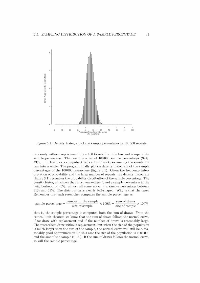
3.1. SAMPLING DISTRIBUTION OF A SAMPLE PERCENTAGE 41
Percentage of households in the sample who own a tablet
Den
sity
(% p
er u
nit o
n th
e ho
rizon
tal a
xis)
0 10 20 30 40 50 60 70 80 90 100
0
2
4
6
8
Figure 3.1: Density histogram of the sample percentages in 100 000 repeats
randomly without replacement draw 100 tickets from the box and compute thesample percentage. The result is a list of 100 000 sample percentages (39%,43%, . . . ). Even for a computer this is a lot of work, so running the simulationcan take a while. The program finally plots a density histogram of the samplepercentages of the 100 000 researchers (figure 3.1). Given the frequency inter-pretation of probability and the large number of repeats, the density histogram(figure 3.1) resembles the probability distribution of the sample percentage. Thedensity histogram shows that most researchers found a sample percentage in theneighborhood of 46%: almost all come up with a sample percentage between31% and 61%. The distribution is clearly bell-shaped. Why is that the case?Remember that each researcher computes the sample percentage as:
sample percentage =number in the sample
size of sample× 100% =
sum of draws
size of sample× 100%
that is, the sample percentage is computed from the sum of draws. From thecentral limit theorem we know that the sum of draws follows the normal curve,if we draw with replacement and if the number of draws is reasonably large.The researchers drew without replacement, but when the size of the populationis much larger than the size of the sample, the normal curve will still be a rea-sonably good approximation (in this case the size of the population is 100 0000and the size of the sample is 100). If the sum of draws follows the normal curve,so will the sample percentage.
42 CHAPTER 3. SAMPLING DISTRIBUTIONS
The 68-95-99.7% rule applies (using expectation instead of average, andSE instead of SD). Most (approximately 99.7%) of the sample percentages fallwithin three standard errors of the expectation, that is, between
46%− 3× 5% and 46% + 3× 5%
or between31% and 61%
Similarly, approximately 95% of the sample percentages fall within two standarderrors of the expectation, that is, between
46%− 2× 5% and 46% + 2× 5%
or between36% and 56%
To summarize the properties of the sampling distribution of the sam-ple percentage:
sample percentage =sum of draws
size of the sample× 100%
1. The sample percentage is an unbiased estimator of the population per-centage:
E(sample percentage) = population percentage
2. The standard error is:
SE(sample percentage) ≈ SD of population√sample size
× 100%
This approximation is good if the population is much larger than thesample. The SD of the population (the box) can be found using theshortcut formula for 0-1 lists. (You don’t have to memorize the formulafor the SE.)
3. If the sample is large, the sampling distribution of the sample percentageapproximately follows the normal curve (central limit theorem).
3.2 Sampling distribution of a sample average
We can now follow the same line of reasoning for the sampling distribution ofa sample average. Suppose a market research firm is interested in the annualhousehold income of the 10 000 households in a small town. Let us model thispopulation as a box with 10 000 tickets. On each ticket the annual income of ahousehold is written:
€ 23 275 € 54 982 € 32 833 . . .
The average annual income of all households in the population is € 27 788;this average is a parameter: a numerical characteristic of the population.The standard deviation of the population is € 8 245 (another parameter). Themarket research firm doesn’t know these parameters, and would like to estimatethe population average by taking a random sample of 100 households. Supposethe sample looks like this:
3.2. SAMPLING DISTRIBUTION OF A SAMPLE AVERAGE 43
€ 26 419 € 47 001 . . . € 14 981 (100 tickets)
The sample average is called a statistic (a numerical characteristic of a sample).The researcher will compute the sample average by adding up the incomes inthe sample and dividing by how many there are:
sample average =€ 26 419 +€ 47 001 + . . .+€ 14 981
100
that is:
sample average =sum of draws
sample size
Just like in the previous example, the sample average is a chance variable: inrepeated samples, the outcome would be different. Just like in the previousexample, the sample average is computed from the sum of draws, so (undercertain conditions) the central limit theorem applies.
It can be shown that the sample average is an unbiased estimator of thepopulation average. The standard error for the sample average is:
SE(sample average) =SE(sum of draws)
sample size
Using the square root law for the SE of the sum of draws, we get:
SE(sample average) ≈√
number of draws× (SD of the box)
sample size
The number of draws is the same thing as the sample size, and the SD of thebox is the same thing as the SD of the population, so we get:
SE(sample average) ≈√
sample size× (SD of population)
sample size
which can be written as:
SE(sample average) ≈ SD(population)√sample size
The SD of the population is given as € 8 245, so the SE for the sample averageis:
SE(sample average) ≈ € 8 245√100
= € 824.5
This means that a researcher who tries to estimate the population average usinga random sample of 100 households is typically going to be off by € 824.5 orso; € 824.5 is the typical size of the chance error that a researcher will make.(Of course, the researcher doesn’t know the SD of the population. If the sampleis large, she can estimate the SD of the population by the SD of the sample.This technique is called the bootstrap. We’ll get back to this when we discussinference.)
In sum, the sampling distribution of the sample average
sample average =sum of draws
sample size
has the following properties:
44 CHAPTER 3. SAMPLING DISTRIBUTIONS
1. The sample average is an unbiased estimator of the population average:
E(sample average) = population average
2. The standard error is
SE(sample average) ≈ SD(population)√sample size
This approximation is good if the population is much larger than thesample. (You don’t have to memorize the formula for the SE.)
3. If the sample is large, the sampling distribution of the sample averageapproximately follows the normal curve (central limit theorem).
3.3 Questions for Review
1. “The sample percentage is a statistic.” Explain.
2. What does the term sampling distribution mean? Explain, using an ex-ample for the sampling distribution of a sample percentage.
3. “The sample percentage is random variable.” Explain.
4. You want to estimate the percentage of a population. Explain what thechance error is.
5. What does the term expectation of the sample percentage mean? Explain,using the concept of repeated samples.
6. What does the term standard error of the sample percentage mean? Ex-plain, using the concept of repeated samples.
7. “The sample percentage is un unbiased estimator of the population per-centage.” Explain.
8. Suppose you would be able to take many large samples (each of the samesize, say, 2500) from the same population. For each sample, you computethe sample percentage. How would the density histogram of the samplepercentage look like (central location, spread, shape)? Explain.
9. Assume that the sample is sufficiently large. How does the probabilitydensity of a sample percentage look like (central location, spread, shape)?Explain.
Chapter 4
Confidence intervals
Carefully review all of chapters 21 (skip section 5) and 23 from Freedman et al.(2007), covered in STA101. Below is a summary of the main ideas. The sum-mary is no substitute for reviewing chapters 21 and 23.
4.1 Estimating a percentage
In a small town there are 10 000 households. A market research agency wantsto find out which percentage of households own a tablet. The population per-centage is an (unknown) parameter. To estimate the parameter, the marketresearch agency interviews a random sample of 100 households. The researchercounts the number of households in the sample who say they own a tablet, andcomputes the sample percentage (a statistic). How reliable is the estimate?
In order to answer this question, we need an appropriate chance model. Wemodel the population as a box of 10 000 tickets. There is a ticket for everyhousehold in the population. This is a case of classifying and counting: weclassify a household as owning a tablet or not owning a tablet, and want tocount the number of households who own a tablet. In cases of classifying andcounting, a 0-1 box is appropriate. For households who own a tablet the valueon the ticket is 1, and for households who own a tablet the value on the ticketis 1. The number of tickets of each kind is unknown:
??? tickets 0 ??? tickets 1
10 000 tickets
The sample is like 100 random draws without replacement from this box. It willlook something like:
{0, 0, 1, 0, 1, 0, 0, . . .} (100 entries)
The number of households in the sample who own a tablet is the sum of draws.The sum of draws is a chance variable: if the researcher had drawn a differentsample of 100 households, the number of households in the sample who own atablet would most likely have been different.
45
46 CHAPTER 4. CONFIDENCE INTERVALS
Suppose that the researcher interviewed 100 random households of whom 41say that they own a tablet. The sample percentage is:
sample percentage =number in the sample
size of sample× 100% =
41
100× 100% = 41%
The sample percentage is called a point estimator of the population percent-age, and the result (41%) is a point estimate.
The decision maker who gave the market research agency the job of estimat-ing the percentage would like to know how reliable the point estimate of 41%is. The sample percentage is a chance variable, subject to sampling variabil-ity: a different sample would most likely have generated a different estimate.We know from the previous chapter that—if the sample is random—the samplepercentage is an unbiased estimator of the population percentage:
E(sample percentage) = population percentage
Intuitively that means that if many researchers all would take a random sampleof 100 households and each would compute a sample percentage, they would getdifferent results, but the results would vary around the population percentage.Some researchers might come up with a sample percentage that is exactly equalto the population percentage, but about half of the researchers would comeup with a sample percentage that underestimates the population percentage,and about half would come up with a sample percentage that overestimates thepopulation percentage. The difference between the sample percentage and thepopulation percentage is called the chance error:
chance error = sample percentage− population percentage
The researcher who came up with the estimate of 41% also made a chance error.Of course, she won’t be able to find how big the chance error exactly is, becauseshe doesn’t know the population percentage. But she does know that she makesa chance error. In the previous chapter we saw that the typical size of thechance error is called the standard error (SE). We also saw that for a samplepercentage, the standard error is:
SE(sample percentage) ≈ SD of population√sample size
× 100%
The bad news is that the researcher doesn’t know the SD of the population.The good news is that statisticians have shown that—provided that the sampleis large—the SD of the sample is a reasonably good estimate of the SD of thepopulation. So for large samples, we can approximate the SE for the samplepercentage by:
SE(sample percentage) ≈ SD of sample√sample size
× 100%
(This is an example of the bootstrap technique.) To find the SD of the sample,the researcher can use the shortcut formula (p. 10):
SD of sample =
√(fraction of
ones
)×(
fraction ofzeroes
)
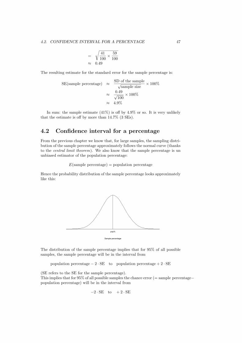
4.2. CONFIDENCE INTERVAL FOR A PERCENTAGE 47
=
√41
100× 59
100≈ 0.49
The resulting estimate for the standard error for the sample percentage is:
SE(sample percentage) ≈ SD of the sample√sample size
× 100%
≈ 0.49√100× 100%
≈ 4.9%
In sum: the sample estimate (41%) is off by 4.9% or so. It is very unlikelythat the estimate is off by more than 14.7% (3 SEs).
4.2 Confidence interval for a percentage
From the previous chapter we know that, for large samples, the sampling distri-bution of the sample percentage approximately follows the normal curve (thanksto the central limit theorem). We also know that the sample percentage is ununbiased estimator of the population percentage:
E(sample percentage) = population percentage
Hence the probability distribution of the sample percentage looks approximatelylike this:
Sample percentage
pop%
The distribution of the sample percentage implies that for 95% of all possiblesamples, the sample percentage will be in the interval from
population percentage− 2 · SE to population percentage + 2 · SE
(SE refers to the SE for the sample percentage).This implies that for 95% of all possible samples the chance error (= sample percentage−population percentage) will be in the interval from
−2 · SE to + 2 · SE
48 CHAPTER 4. CONFIDENCE INTERVALS
Put in a different way, for 95% of all possible samples the chance error (withoutthe minus sign) will be smaller than 2 · SE. Or: for 95% of all possible samples,the interval from
sample percentage− 2 · SE to sample percentage + 2 · SE
will cover the population percentage. This interval is called the 95%-confidenceinterval for the population percentage.
There is a shorter notation for the 95%-confidence interval:
sample percentage± 2 · SE(sample percentage)
The term 2 · SE is called the margin of error.The researcher found an estimate of 41% and a standard error of about 4.9%.
The sample was reasonably large (100), so it’s safe to assume that the normalcurve is a good approximation of the probability distribution of the samplepercentage. Hence the 95%-confidence interval for the population percentage isthe interval between:
41%− 2× 4.9% and 41% + 2× 4.9%
41%− 9.8% and 41% + 9.8%
31.2% and 50.8%
In sum: the sample estimate (41%) is off by 4.9% or so. You can be about95% confident that the the interval from 31.2% to 50.8% covers the populationpercentage.
To compute a confidence interval for a population percentage with the TI-84, do STAT→ TESTS→ 1-PropZInt (one-proportion z interval). The z refersto the fact that we use the normal approximation (central limit theorem). Thevalue x that you have to enter is the number of times the event occurs in thesample (41 in the example); n is the sample size (100 in the example); C-Levelstands for confidence level: for a 95% confidence interval enter .95 (the defaultvalue). The procedure gives the sample proportion (p) and the boundaries of theconfidence interval as decimal fractions; to get percentages multiply by 100%.The confidence interval provided by the TI-84 (and by statistical software) dif-fers somewhat from what you find using the formula above. Don’t worry: ourformula gives a good approximation.
4.3 Interpreting a confidence interval
Carefully read Freedman et al. (2007, section 3 pp. 383–386). It’s importantthat you understand the correct interpretation of a confidence interval.
Suppose you have a fish bowl with 100 000 marbles (the population): 80 000red marbles and 20 000 blue ones. The proportion of red marbles in the popu-lation is:
population proportion =80 000
100 000× 100% = 80%
The population proportion is a parameter. Now you conduct the following ex-periment. You hire a researcher and tell her that you don’t know the proportionof red marbles, and that you would like her to estimate the proportion of red
4.3. INTERPRETING A CONFIDENCE INTERVAL 49
marbles from a random sample of 2 500 marbles. The researcher takes up thejob: she takes a simple random sample of 2 500 marbles, counts the number ofred marbles in the sample, and computes a the sample proportion as a pointestimate of the population proportion:
sample percentage =number of red marbles in the sample
100 000× 100%
Because the sample is large (and hence the central limit theorem applies), shecan compute a 95%-confidence interval:
sample percentage± 2 · SE(sample percentage)
The sample percentage is a chance variable: the outcome depends on the sampleshe took. Had she taken another sample of size 2 500, the sample percentagewould most likely have been different (the population percentage would stillhave been 80%, of course): the chance is in the sampling variability, not in theparameter. Suppose that she finds a confidence interval like that in case (1):
Three confidence intervals (x = the parameter)
(1) |------x--------| (covers)
(2) x |----------| (does not cover)
(3) |----------| x (does not cover)
Confidence interval (1) covers the population percentage (the researcher willof course not know this because she doesn’t know the population percentage).
Now you hire another researcher, and you tell him the same thing: thatyou don’t know the proportion of red marbles, and that you would like him toestimate the proportion of red marbles from a random sample of 2 500 marbles.Because he will draw a different sample, he will come up with a different pointestimate, a different SE, and a different confidence interval. The confidence in-terval may cover the population percentage, but—due to sampling variability—it may not: the interval may be too far too the right (case (2)) or too far to theleft (case (3)) (Freedman et al. (2007, p. 384) call confidence intervals that don’tcontain the parameter “lemons”). Again, the researcher doesn’t know whetherthe confidence interval he computed covers the population percentage: it may(case (1)), or it may not (cases (2) or (3)).
You can find out what happens in repeated samples if you repeat the exper-iment many times (say: you hire 100 researchers) and plot the resulting 95%-confidence intervals. A computer simulation posted on the course web site doesexactly that (interpreting-a-confidence-interval-for-a-percentage.R).The script generates a diagram like figure 4.1 (compare to figure 1 in Freedmanet al. (2007, p. 385)). Each horizontal line represents a 95%-confidence intervalcomputed by a researcher. The vertical line shows the population percentage.Run the script a number of times (and make sure you understand what thescript does). Count the number of lemons in each run. Is there a pattern?
In sum: if 100 researchers would each take a simple random sample of 100marbles, and each computes a 95%-confidence interval, we get 100 confidenceintervals. The confidence intervals differ because of sampling variability. Forabout 95% of samples, the interval
sample percentage± 2 · SE(sample percentage)
covers the population percentage, and for the other 5% is does not.
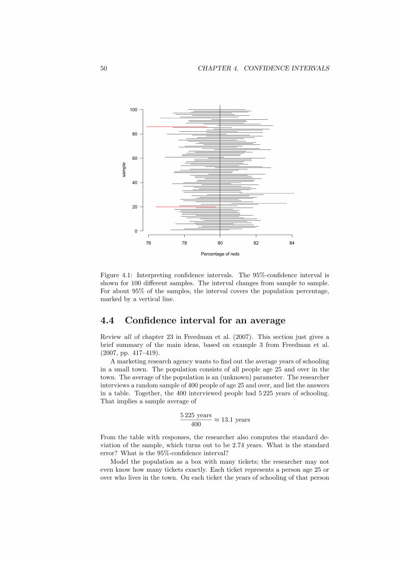
50 CHAPTER 4. CONFIDENCE INTERVALS
76 78 80 82 84
0
20
40
60
80
100
Percentage of reds
sample
Figure 4.1: Interpreting confidence intervals. The 95%-confidence interval isshown for 100 different samples. The interval changes from sample to sample.For about 95% of the samples, the interval covers the population percentage,marked by a vertical line.
4.4 Confidence interval for an average
Review all of chapter 23 in Freedman et al. (2007). This section just gives abrief summary of the main ideas, based on example 3 from Freedman et al.(2007, pp. 417–419).
A marketing research agency wants to find out the average years of schoolingin a small town. The population consists of all people age 25 and over in thetown. The average of the population is an (unknown) parameter. The researcherinterviews a random sample of 400 people of age 25 and over, and list the answersin a table. Together, the 400 interviewed people had 5 225 years of schooling.That implies a sample average of
5 225 years
400≈ 13.1 years
From the table with responses, the researcher also computes the standard de-viation of the sample, which turns out to be 2.74 years. What is the standarderror? What is the 95%-confidence interval?
Model the population as a box with many tickets; the researcher may noteven know how many tickets exactly. Each ticket represents a person age 25 orover who lives in the town. On each ticket the years of schooling of that person
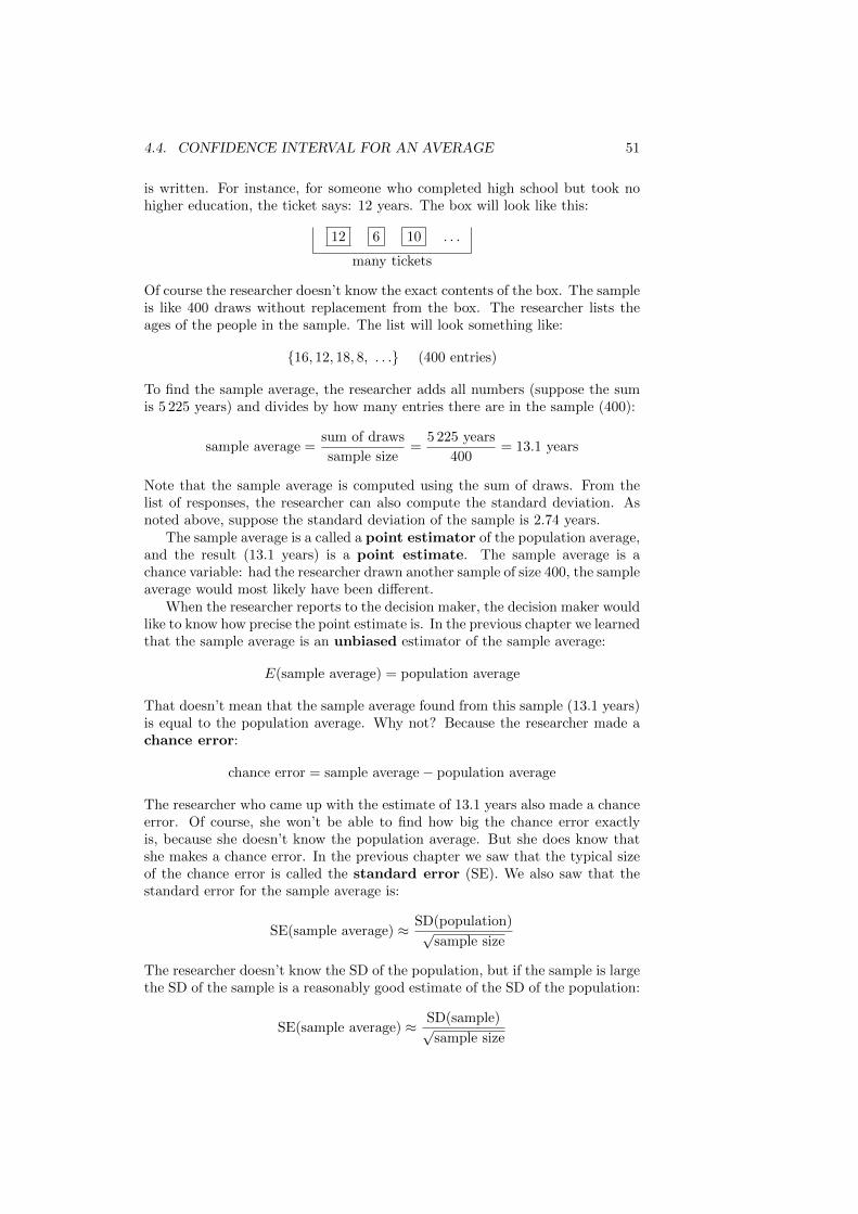
4.4. CONFIDENCE INTERVAL FOR AN AVERAGE 51
is written. For instance, for someone who completed high school but took nohigher education, the ticket says: 12 years. The box will look like this:
12 6 10 . . .
many tickets
Of course the researcher doesn’t know the exact contents of the box. The sampleis like 400 draws without replacement from the box. The researcher lists theages of the people in the sample. The list will look something like:
{16, 12, 18, 8, . . .} (400 entries)
To find the sample average, the researcher adds all numbers (suppose the sumis 5 225 years) and divides by how many entries there are in the sample (400):
sample average =sum of draws
sample size=
5 225 years
400= 13.1 years
Note that the sample average is computed using the sum of draws. From thelist of responses, the researcher can also compute the standard deviation. Asnoted above, suppose the standard deviation of the sample is 2.74 years.
The sample average is a called a point estimator of the population average,and the result (13.1 years) is a point estimate. The sample average is achance variable: had the researcher drawn another sample of size 400, the sampleaverage would most likely have been different.
When the researcher reports to the decision maker, the decision maker wouldlike to know how precise the point estimate is. In the previous chapter we learnedthat the sample average is an unbiased estimator of the sample average:
E(sample average) = population average
That doesn’t mean that the sample average found from this sample (13.1 years)is equal to the population average. Why not? Because the researcher made achance error:
chance error = sample average− population average
The researcher who came up with the estimate of 13.1 years also made a chanceerror. Of course, she won’t be able to find how big the chance error exactlyis, because she doesn’t know the population average. But she does know thatshe makes a chance error. In the previous chapter we saw that the typical sizeof the chance error is called the standard error (SE). We also saw that thestandard error for the sample average is:
SE(sample average) ≈ SD(population)√sample size
The researcher doesn’t know the SD of the population, but if the sample is largethe SD of the sample is a reasonably good estimate of the SD of the population:
SE(sample average) ≈ SD(sample)√sample size
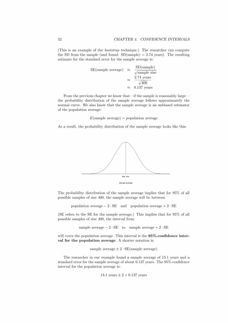
52 CHAPTER 4. CONFIDENCE INTERVALS
(This is an example of the bootstrap technique.) The researcher can computethe SD from the sample (and found: SD(sample) = 2.74 years). The resultingestimate for the standard error for the sample average is:
SE(sample average) ≈ SD(sample)√sample size
≈ 2.74 years√400
≈ 0.137 years
From the previous chapter we know that—if the sample is reasonably large—the probability distribution of the sample average follows approximately thenormal curve. We also know that the sample average is an unbiased estimatorof the population average:
E(sample average) = population average
As a result, the probability distribution of the sample average looks like this:
Sample average
pop. ave.
The probability distribution of the sample average implies that for 95% of allpossible samples of size 400, the sample average will be between
population average− 2 · SE and population average + 2 · SE
(SE refers to the SE for the sample average.) This implies that for 95% of allpossible samples of size 400, the interval from
sample average− 2 · SE to sample average + 2 · SE
will cover the population average. This interval is the 95%-confidence inter-val for the population average. A shorter notation is:
sample average± 2 · SE(sample average)
The researcher in our example found a sample average of 13.1 years and astandard error for the sample average of about 0.137 years. The 95%-confidenceinterval for the population average is:
13.1 years± 2× 0.137 years
4.5. DON’T CONFUSE SE AND SD 53
or:
13.1 years± 0.274 years
The margin of error (with a confidence level of 95%) is 0.274 years. So the95%-confidence interval for the population average is the interval from:
13.1 years− 0.274 years to 13.1 years + 0.274 years
or from:
12.83 years to 13.37 years
In sum: the sample estimate (13.1 years) is off by 0.137 years or so. You canbe about 95% confident that the interval from 12.83 years to 13.37 years coversthe population average.
To compute a confidence interval for a population average with the TI-84, doSTAT → TESTS → ZInterval. The z refers to the fact that we use the normalapproximation (central limit theorem). The value σ (sigma) that you have toenter is the standard deviation of the population; as you don’t know the standarddeviation of the population, enter the sample standard deviation instead (youare using the bootstrap, but remember that the bootstrap only works when thesample is large). In the example, the standard deviation of the sample was 2.74years. The value x (x-bar) that you have to enter is the sample average (13.1years in the example) and n is the sample size (400 in the example). C-Level
stands for confidence level; for a 95% confidence interval enter .95.
4.5 Don’t confuse SE and SD
The researcher computed two numbers: she found that the SD of the samplewas 2.74 years, and that the SE for the sample average was 0.137 years. Thesetwo numbers tell two different stories (Freedman et al., 2007, p. 417):
– the SD says how far schooling is from the average—for typical people.
– the SE says how far the sample averages are from the population average—for typical samples.
People who confuse SE and SE often think that 95% of the people have schoolingin the range 13.1 years ± 0.274 years (13.1 years ± 2 · SE). That is wrong.The interval 13.1 years± 0.274 years covers only a very small part of the yearsof schooling: the SD is about 2.74 years. The confidence interval measuressomething else: if many researchers each take a sample of 400 people, and eachcomputes a 95%-confidence interval, then about 95% of the confidence intervalswill cover the population average; the other 5% of the confidence intervals won’t.The term “confidence” reminds you of the fact that the chance is in the samplevariability; the population average doesn’t change.
4.6 Questions for Review
1. Why do we need to use the bootstrap when estimating the standard errorfor a percentage?
54 CHAPTER 4. CONFIDENCE INTERVALS
2. What is the margin or error (at a 95% confidence level) for the populationpercentage? For a population mean?
3. Suppose the decision maker requires a level of confidence higher than 95%(say, 99%). Would the margin or error be bigger, smaller, or the same aswith a level of confidence of 95%? Explain.
4. Suppose the decision maker is happy with a confidence level of 95% butwants a smaller margin of error. What should you do? Explain.
5. What is the difference between the standard deviation of the sample andthe standard error of the sample average? Explain.
6. A researcher computes a 95%-confidence interval for the mean. Right orwrong: 95 percent of the values in the sample fall within this interval.Explain.
7. A researcher computes a 95%-confidence interval for the mean. Explainwhat the meaning of the interval is, using the concept of repeated samples.Add a sketch.
4.7 Exercises
Work the following exercises from Freedman et al. (2007), chapter 21: A–1; A–2and B–2(a); A–3; A–4, A–5; A–9; B–1; B–4; C–5; C–6; D–1; D–2.
Work the following exercises from Freedman et al. (2007), chapter 23: A–1;A–2; A–3; A–4; A–5; A–6; A–7; A–8; A–9; A–10; B–1; B–2; B–3; B–4; B–5;B–6; B–7; C–1; C–2; C–3; C–4; D–1; D–2; D–3; D–4.
Chapter 5
Hypothesis tests
Read Freedman et al. (2007, Ch. 26, 29). Leave section 6 of chapter 26 (pp.488–495) for later.
Questions for Review
1. Freedman et al. (2007, Ch. 26) repeatedly use the term observed difference.Explain (the difference between what and what?).
2. What is a test statistic? Explain using an example.
3. What is the observed significance level (or P -value)?
4. When the P -value is less than 1% (so the results is “highly statisticallysignificant”), what does this imply for the null hypothesis?
Exercises
Work the following exercises from Freedman et al. (2007), chapter 26: Set A: 4,5. Set B: 1, 2, 5. Set C: 1, 2, 4, 5. Set D: all. Set E: 1–5, 7, 10. Set F: 1–4.Review Exercises: 1–5, 7, 8.
Work the following exercises from Freedman et al. (2007), chapter 29: Set A: 1,2. Set C: 1, 4, 5, 7. Set D: 2, 5.
55

56 CHAPTER 5. HYPOTHESIS TESTS
Chapter 6
Hypothesis tests for smallsamples
Read Freedman et al. (2007, Ch. 26, section 6).
The spectrophotometer example used by Freedman et al. (2007, Ch. 26, pp.488–489) is rather complicated. Consider instead the following story (that usesthe same numbers): A large chain of gas stations sells refrigerated cans of Coke.On average the chain sells about 70 per day per station. The manager noticesthat a competing chain has increased the price of a refrigerated can of Coke,and wonders whether as a result she now is on average selling more than before.She records the number of cans sold by five randomly selected gas stations fromthe chain:
78 83 68 72 88
Four out of five of these numbers are higher than 70, and some of them by quitea bit. Can this explained on basis of chance variation? Or did the mean numberof cans sold per gas station increase?
(You can now construct the box model, formulate the null and alternativehypothesis, and compute the test statistic. Continue reading on p. 490 andreplace ppm by cans.)
Questions for Review
1. When the sample is small, there is extra uncertainty. How does the testprocedure take this extra uncertainty into account (two ways)?
2. What are the properties of Student’s t-curve? Compare with the normalcurve.
3. When should Student’s curve be used?
57

58 CHAPTER 6. HYPOTHESIS TESTS FOR SMALL SAMPLES
Exercises
1. A long series of the number of refrigerated cans of Coca Cola sold by alarge chain of gas stations averages to 253 cans per station per week. Followingan advertising campaign by Pepsi Cola, the manager of the chain collects datafrom ten randomly selected gas stations. She finds that the number of cans ofCoca Cola in the sample averages 245 cans, and that the standard deviation is9 cans. Did the mean fall, or is this chance variation? (This is a variant of SetF: exercise 6.)2. (I will add more exercises later.)
Chapter 7
Hypothesis tests on twoaverages
Read Freedman et al. (2007, Ch. 27).
Questions for Review
1. What is the standard error for a difference? Explain using a box model.Give an example of a case where the formula from for the SE for a differ-ence used in the textbook does not apply.
2. What are the assumptions of the two-sample z-test for comparing twoaverages? Can you think of examples when you want to compare twoaverages but a z-test is not appropriate?
3. When should the χ2-test be used, as opposed to the z-test?
4. What are the six ingredients of a χ2-test?
Exercises
Work the following exercises from Freedman et al. (2007), chapter 28: Set A: 1(use the TI-84), 2 (use the TI-84), 3, 4, 7, 8. Set C: 2.
59

60 CHAPTER 7. HYPOTHESIS TESTS ON TWO AVERAGES
Chapter 8
Correlation
Read Freedman et al. (2007, Ch. 8, 9). Skip section 3 (“The SD line,” pp.130–132) from Freedman et al. (2007, Ch. 8).
Questions for Review
1. If you want to summarize a scatter diagram, which five numbers wouldyou report?
2. What are the properties of the coefficient of correlation?
3. How do you compute a coefficient of correlation?
4. What are the units of a coefficient of correlation?
5. Which data manipulations will not affect the coefficient of correlation?
6. In which cases can a coefficient of correlation be misleading? Make sketchesto illustrate your point.
7. What are ecological correlations? Why can they be misleading?
8. What is the connection between correlation and causation?
Exercises
Work the following exercises from Freedman et al. (2007), chapter 8: Set A: 1,6. Set B: 1, 2, 9. Set D: 1.Work the following exercises from Freedman et al. (2007), chapter 9: Set C: 1,2. Set D: 1, 2. Set E: 2, 3, 4.
61

62 CHAPTER 8. CORRELATION
Chapter 9
Line of best fit
Read Freedman et al. (2007), chapters 10 (introduction pp. 158–161 only), 11,12.
Note
The formula sheet has the following formula for the y-intercept of the line ofbest fit:
y-intercept = (ave of y)− slope× (ave of x)
This formula is obtained as follows. The equation of the line of best fit is:
predicted value of y = slope× x+ y-intercept
As the line of best fit passes through the point of averages (ave of x, ave of y),we know that:
ave of y = slope× (ave of x) + y-intercept
Solving this expression for the y-intercept yields:
y-intercept = (ave of y)− slope× (ave of x)
Q.E.D.
Questions for Review
1. What does line of best fit measure?
2. On the average, what happens to y if there is an increase of one SD in x?
3. Suppose you have a scatter plot with a line of best fit. What is the error(or residual) of a given point of the scatter plot? Illustrate.
4. What does the standard error (or r.m.s. error) of regression measure?
5. What is the standard error (or r.m.s. error) of regression computed?
6. What properties do the residuals have?
63
64 CHAPTER 9. LINE OF BEST FIT
7. What is the difference between a homoscedastic and a heteroscedasticscatter diagram? Illustrate.
8. If you run an observational study, can the line of best fit be used to predictthe results of interventions? Why (not)?
9. In what sense is the line of best fit the line that gives the best fit?
Exercises
Work the following exercises from Freedman et al. (2007), chapter 10: Set A: 1,2, 4.
Work the following exercises from Freedman et al. (2007), chapter 11: Set A: 3,4, 7. Set D: 2, 3.
Work the following exercises from Freedman et al. (2007), chapter 12: Set A: 1,2.
Additional exercise
Table 9.1 shows the heights and weights of 30 students (the file is available asstudents.csv on the course web site). The average height is 174.03 cm andthe SD is 9.63 cm. The average weight is 65.13 kg and the SD is 13.36 kg. Thecoefficient of correlation between height and weight is 0.75.
(a) Make a scatter plot (12 cm tall and 10 cm wide) on squared or graphingpaper. Truncate the horizontal axis at 150 cm and let it run to 200 cm (2cm on the page is 10 cm of a student’s height). Truncate the vertical axisat 40 kg and let it run to 100 kg (2 cm on the page is 10 kg of a student’sweight). In class, plot 10 points or so (you can plot the other points later).
(b) Show the point of averages, the run, the rise, and the second point of theline of best fit. With the two points, draw the line of best fit.
(c) Compute the slope and the y-intercept of the line of best fit. Report theline of best fit (use the actual variable names and pay attention to theunits of measurement).
(d) Find the predicted weight for the student with a height of 190 cm. Illus-trate in the scatter plot.
(e) Find the residual for the student with a height of 190 cm. Illustrate in thescatter plot.
(f) The r.m.s. error is 8.65 kg (you can verify this using the R script referredto below). Draw the line of best fit plus two r.m.s. errors and minus twor.m.s. errors (cf. Freedman et al. (2007, p. 183). Add all 30 points to thescatter and count which percentage of points lies within two r.m.s. errorsof the line of best fit. Does the rule of thumb give a good approximation?
65
Use R Commander to find the descriptive statistics (average and standard devi-ation), the coefficient of correlation, the equation of the line of best fit, and tomake a scatter plot with the line of best fit. To get the averages and SDs, selectin the menu: Statistics→ Summaries→ Numerical summaries. To get the coef-ficient of correlation, select : Statistics→ Summaries→ Correlation matrix. Toget the scatter plot with the line of best fit, select: Graphs → Scatterplot. . . Inthe Data tab, select the x-variable and the y-variable. In the Options tab, onlyselect the Plot option Least-squares line (unselect other items that may be se-lected by default). In the Identify Points options, select Do not identify. Toget the coefficients of the line of best fit, select : Statistics → Fit models →Linear regression. . . Select the correct response variable (the dependent vari-able; the variable on the y-axis of the scatter plot) and explanatory variable(the independent variable, the variable on the x-axis of the scatter plot).
Compare your outcomes with the outcomes obtained using R. (Alterna-tively, the R script R-script-Scatter-plot-of-heights-and-weights.R onthe course web site computes the line of best fit and makes the scatter plot.)
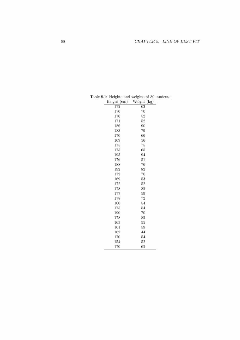
66 CHAPTER 9. LINE OF BEST FIT
Table 9.1: Heights and weights of 30 studentsHeight (cm) Weight (kg)
172 63170 70170 52171 52186 90183 79170 66169 56175 75175 65195 94176 51188 76192 82172 70169 53172 52178 85177 59178 72160 54175 54190 70178 85163 55161 59162 44170 54154 52170 65
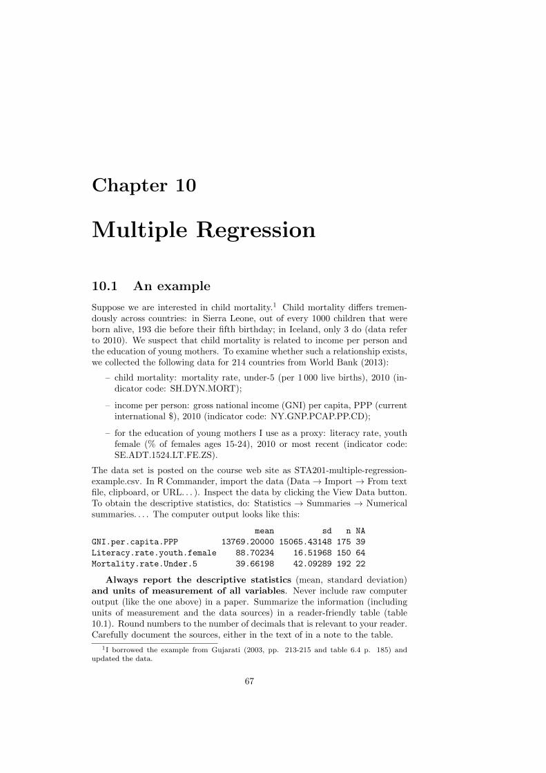
Chapter 10
Multiple Regression
10.1 An example
Suppose we are interested in child mortality.1 Child mortality differs tremen-dously across countries: in Sierra Leone, out of every 1000 children that wereborn alive, 193 die before their fifth birthday; in Iceland, only 3 do (data referto 2010). We suspect that child mortality is related to income per person andthe education of young mothers. To examine whether such a relationship exists,we collected the following data for 214 countries from World Bank (2013):
– child mortality: mortality rate, under-5 (per 1 000 live births), 2010 (in-dicator code: SH.DYN.MORT);
– income per person: gross national income (GNI) per capita, PPP (currentinternational $), 2010 (indicator code: NY.GNP.PCAP.PP.CD);
– for the education of young mothers I use as a proxy: literacy rate, youthfemale (% of females ages 15-24), 2010 or most recent (indicator code:SE.ADT.1524.LT.FE.ZS).
The data set is posted on the course web site as STA201-multiple-regression-example.csv. In R Commander, import the data (Data → Import → From textfile, clipboard, or URL. . . ). Inspect the data by clicking the View Data button.To obtain the descriptive statistics, do: Statistics → Summaries → Numericalsummaries. . . . The computer output looks like this:
mean sd n NA
GNI.per.capita.PPP 13769.20000 15065.43148 175 39
Literacy.rate.youth.female 88.70234 16.51968 150 64
Mortality.rate.Under.5 39.66198 42.09289 192 22
Always report the descriptive statistics (mean, standard deviation)and units of measurement of all variables. Never include raw computeroutput (like the one above) in a paper. Summarize the information (includingunits of measurement and the data sources) in a reader-friendly table (table10.1). Round numbers to the number of decimals that is relevant to your reader.Carefully document the sources, either in the text of in a note to the table.
1I borrowed the example from Gujarati (2003, pp. 213-215 and table 6.4 p. 185) andupdated the data.
67
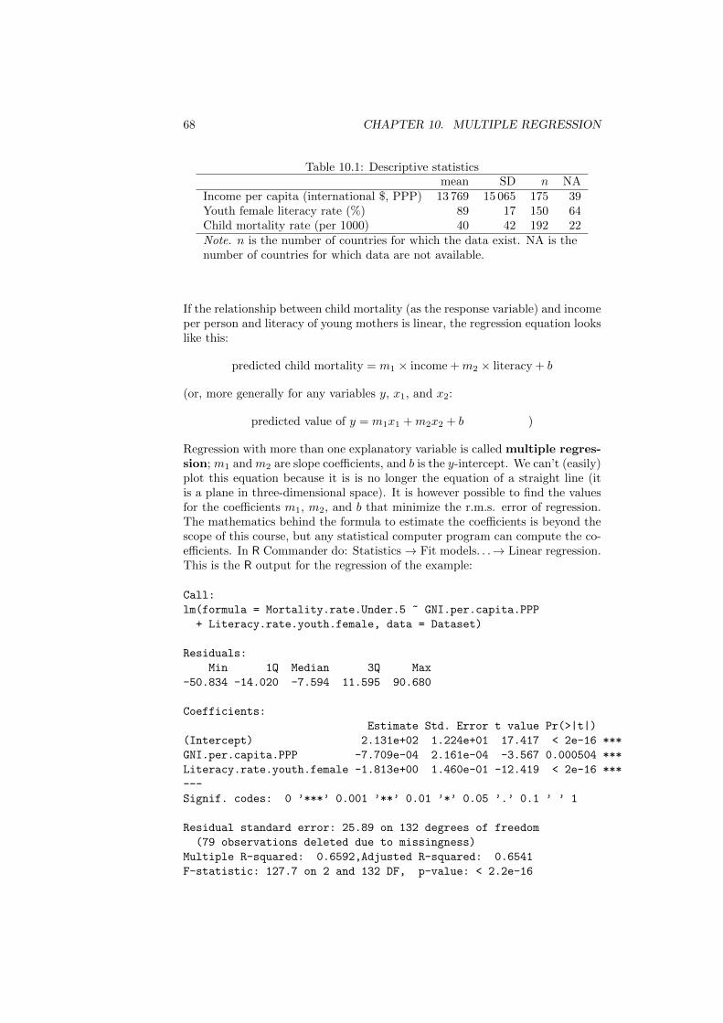
68 CHAPTER 10. MULTIPLE REGRESSION
Table 10.1: Descriptive statisticsmean SD n NA
Income per capita (international $, PPP) 13 769 15 065 175 39Youth female literacy rate (%) 89 17 150 64Child mortality rate (per 1000) 40 42 192 22Note. n is the number of countries for which the data exist. NA is thenumber of countries for which data are not available.
If the relationship between child mortality (as the response variable) and incomeper person and literacy of young mothers is linear, the regression equation lookslike this:
predicted child mortality = m1 × income +m2 × literacy + b
(or, more generally for any variables y, x1, and x2:
predicted value of y = m1x1 +m2x2 + b )
Regression with more than one explanatory variable is called multiple regres-sion; m1 and m2 are slope coefficients, and b is the y-intercept. We can’t (easily)plot this equation because it is is no longer the equation of a straight line (itis a plane in three-dimensional space). It is however possible to find the valuesfor the coefficients m1, m2, and b that minimize the r.m.s. error of regression.The mathematics behind the formula to estimate the coefficients is beyond thescope of this course, but any statistical computer program can compute the co-efficients. In R Commander do: Statistics→ Fit models. . .→ Linear regression.This is the R output for the regression of the example:
Call:
lm(formula = Mortality.rate.Under.5 ~ GNI.per.capita.PPP
+ Literacy.rate.youth.female, data = Dataset)
Residuals:
Min 1Q Median 3Q Max
-50.834 -14.020 -7.594 11.595 90.680
Coefficients:
Estimate Std. Error t value Pr(>|t|)
(Intercept) 2.131e+02 1.224e+01 17.417 < 2e-16 ***
GNI.per.capita.PPP -7.709e-04 2.161e-04 -3.567 0.000504 ***
Literacy.rate.youth.female -1.813e+00 1.460e-01 -12.419 < 2e-16 ***
---
Signif. codes: 0 ’***’ 0.001 ’**’ 0.01 ’*’ 0.05 ’.’ 0.1 ’ ’ 1
Residual standard error: 25.89 on 132 degrees of freedom
(79 observations deleted due to missingness)
Multiple R-squared: 0.6592,Adjusted R-squared: 0.6541
F-statistic: 127.7 on 2 and 132 DF, p-value: < 2.2e-16
10.2. INTERPRETATION OF THE SLOPE COEFFICIENTS 69
(The regression output of other statistical software is similar.)The first line shows the regression equation. lm stands for linear model. The
variable before the tilde (~) is the dependent variable (the variable you want topredict; y in the mathematical notation). Following the tilde are the indepen-dent variables (x1 and x2 in the mathematical notation). Think of the tilde asmeaning “is predicted by”: y ~ x1 + x2 means “y is predicted by x1 and x2.”The column Estimate in the Coefficients table gives the estimated coefficientsof the regression equation. We discuss the other columns of the Coefficients
table in the chapter on inference for regression. Residual standard error isthe r.m.s. error of regression (calculated slightly differently than in Freedmanet al. (2007, pp. 185-187), so the result may differ somewhat; if the number ofcases is small, the difference may be quite large). The r.m.s. error of regressionmeasures by how much the predicted value for y typically deviates from theactual value. Report the equation using the actual variable names, not y, x1,and x2:
predicted child mortality = 213.1− 0.00077× income− 1.813× literacy
The r.m.s. error of regression is 25.89: this is by how much the predictedvalue for child mortality typically deviates from the actual value. The R outputreports that 79 observations were deleted due to missingness, so the regressionuses only 135 (= 214− 79) countries.
10.2 Interpretation of the slope coefficients
In a controlled experiment, the researcher controls for variables other than thetreatment variable. In observational studies however, usually the variables y,x1, and x2 all vary at the same time. One of the strengths of multiple regressionis that it allows to isolate the association between the dependent variable (y)and one of the independent variables, keeping the other independent variablesin the equation constant. The slope coefficient m1 measures by how muchthe predicted value of y changes if x1 increases by one unit, keeping all otherindependent variables in the equation constant. (In this case, there is only oneother independent variable: x2.) Similarly, the slope coefficient m2 measures byhow much the predicted value of y changes if x2 increases by one unit, keeping allother independent variables in the equation constant. (If you took calculus: m1
is the partial derivative of y with regards to x1, and m2 is the partial derivativeof y with regards to x2.)
For the numerical example, the slope coefficient of income per capita showsthat a one unit (in this case: a one dollar) increase in income per capita isassociated with decrease in the predicted child mortality rate by 0.00077 units(children per 1000 life births). Note that the slope coefficients have as units ofmeasurement: units of the response variable per units of the independent vari-able. This is clear from the formula for the slope coefficient in simple regression:
slope =r × SD of y
SD of x
and is still true for the slope coefficients in multiple regression. In practice, theunits of measurement of the coefficients in multiple regression are often omittedwhen the equation is reported.
70 CHAPTER 10. MULTIPLE REGRESSION
On the scale of income per capita—that typically ranges from $1 950 (firstquartile) to $19 150 (third quartile)—a $1 increase is not very meaningful; a$1000 increase is more relevant. So let us reinterpret the slope coefficient ofincome per capita: the regression predicts that a $1000 increase of income percapita is associated with a decrease by 0.77 in the predicted number of childrenper 1000 who die before their fifth birthday. The slope coefficient of the literacyrate of youth females shows that with a 1 percentage point increase in theliteracy rate of youth females is associated a drop of the predicted child mortalityrate by 1.813 units, that is, a decrease by 1.813 in the number of children per1000 who die before their fifth birthday.
Be careful when drawing policy conclusions from an observational study. Itis tempting to infer from the regression that a policy that increases the femaleyouth literacy rate by 10 percentage points would cause child mortality to de-crease by about 18. However, “[T]he slope cannot be relied on to predict howy would respond if you intervene to change the value of x. If you run an ob-servational study, the regression line only describes the data you see. The linecannot be relied on for predicting the results of interventions.”(Freedman et al.,2007, p. 206).
10.3 Coefficient of determination
The following sketch shows in a scatter plot of a simple regression the actualvalue of y, the predicted value of y, and the average of y (many textbooks usethe following notation: y for the actual value, y for the predicted value, and yfor the average):
yactual-ypredicted-yave.pdf
Take a closer look at the following vertical differences:
actual value for y − ave y
predicted value for y − ave y
actual value for y − predicted value for y = residual
Note that:
actual value for y−ave y = (predicted value for y−ave y)+(actual value for y−predicted value for y)
10.3. COEFFICIENT OF DETERMINATION 71
Define the total sum of squares (TSS) as the sum of squared deviationsbetween each actual value for y and the average of y:
TSS = sum of (actual values for y − ave y)2
The total sum of squares is a measure of the variation of y around its average.The explained sum of squares (ESS) is the sum of squared deviations betweeneach predicted value for Y and the average of y:
ESS = sum of (predicted values for y − ave y)2
The explained sum of squares is a measure of the variation of y around itsaverage that is explained by the regression equation.The residual sum of squares (RSS) is the sum of squared residuals:
RSS = sum of (actual values for y − predicted values for y)2
When we computed the r.m.s. of regression we already encountered the resid-ual sum of squares as the numerator of the fraction under the square root inFreedman et al. (2007, p. 182):
RSS = (error #1)2 + (error #2)2 + . . .+ (error #n)2
It can be shown (proof omitted) that the total sum of squares is equal to theexplained sum of squares plus the residual sum of squares:
TSS = ESS + RSS
Divide both sides by TSS:
1 =ESS
TSS+
RSS
TSSThe term RSS/TSS measures which proportion of the variation in y aroundits average is left unexplained by the regression. The term ESS/TSS showswhich proportion of the variation in y around its average is explained by theregression. We call this proportion the coefficient of determination (notation:R2): the coefficient of determination (R2) measures the proportion of thevariation in the dependent variable that is explained by the regressionequation:
R2 =ESS
TSS=
sum of (predicted values for y − ave y)2
sum of (actual values of y − ave y)2
The coefficient of determination is a measure of the goodness-of-fit of theestimated regression equation. You don’t have to memorize the formula, butyou do have to know the meaning of R2.
In the R computer output, the coefficient of determination is reported asMultiple R-squared. In the example, R2 is equal to 0.6592; this means thatthe estimated regression equation (for the 132 countries in the data set) explainsabout two-thirds (66%) of the variation of child mortality around its mean. Thatis quite a lot: the estimated regression equation fit the data quite well.
It can be shown that for simple regression (with only one independent vari-able), R2 is equal to the coefficient of correlation (r) squared: R2 = r2. Formultiple regression, that is not the case (there are several coefficients of correla-tion, one for each independent variable: between y and x1, between y and x2).That is why for multiple regression the coefficient of determination is writtenas capital R2, not lowercase r2.
72 CHAPTER 10. MULTIPLE REGRESSION
10.4 Questions for Review
1. How does multiple regression differ from simple regression?
2. What is the interpretation of the coefficient of one of the variables at theright-hand side of a multiple regression equation?
3. How is a residual in a multiple regression model computed?
4. What is the total sum of squares? What is the explained sum of squares?What is the residual sum of squares?
5. How is the coefficient of determination of a regression model computed?
6. What is the meaning of the coefficient of determination? If the coefficientof determination of a regression model is equal to 0.67, what does thismean?
10.5 Exercises
1. For 14 systems analysts, their annual salaries (in $), years of experience, andyears of postsecondary education were recorded (Kazmier, 1995, table 15.2 p.275). Below is the computer output for the descriptive statistics and a multipleregression of the annual salaries on the years of experience and the years ofpostsecondary education.
(a) Download the data (Kazmier1995-table-15-2.csv) from the course website. Compute the descriptive statistics and run the regression in R withR Commander. You should get the same output as shown below.
mean sd n
annual.salary 57000.000000 3513.49048 14
years.of.experience 5.928571 2.94734 14
years.of.postsecondary.education 4.071429 1.12416 14
lm(formula = annual.salary ~ years.of.experience
+ years.of.postsecondary.education,
data = Dataset)
Residuals:
Min 1Q Median 3Q Max
-3998.6 -1379.1 -158.7 1067.9 4343.6
Coefficients:
Estimate Std. Error t value Pr(>|t|)
(Intercept) 45470.9 2731.2 16.649 3.78e-09 ***
years.of.experience 842.3 207.7 4.056 0.0019 **
years.of.postsecondary.education 1605.3 544.4 2.948 0.0132 *
---
Signif. codes: 0 ’***’ 0.001 ’**’ 0.01 ’*’ 0.05 ’.’ 0.1 ’ ’ 1
10.5. EXERCISES 73
Residual standard error: 2189 on 11 degrees of freedom
Multiple R-squared: 0.6715,Adjusted R-squared: 0.6118
F-statistic: 11.24 on 2 and 11 DF, p-value: 0.002192
(b) Report the equation like you would in a paper.
(c) Explain what the coefficients, the “residual standard error” and the valueof R2 mean. Pay attention to the units of measurement.
(d) Predict the annual salary of a systems analyst with four years of educationand three years of experience.
(e) Would it be meaningful to use the regression equation to predict the annualsalary of a systems analyst with four years of education and twenty yearsof experience? Why (not)?

74 CHAPTER 10. MULTIPLE REGRESSION
Chapter 11
Hypothesis tests forregression coefficients
Until now we have used regression as a tool of descriptive statistics: as a methodto describe relationships between variables. Under certain conditions, regres-sion can also be a tool of inferential statistics: we can test hypotheses aboutregression coefficients. This chapter explains when and how.
11.1 Population regression function
Consider the following (hypothetical) example (drawn from Gujarati (2003,Chapter 2)). Suppose that during one week a population of 60 families had theweekly income and the weekly consumption expenditure shown in table 11.1.The data set is posted on the course web site as Gujarati-2003-table-2-1.csv;the R script as two-variable-regression-analysis.R. Figure 11.1 shows the scat-ter plot. There are ten income groups (families with incomes of $80, $100,$120,. . . , and $260).
75
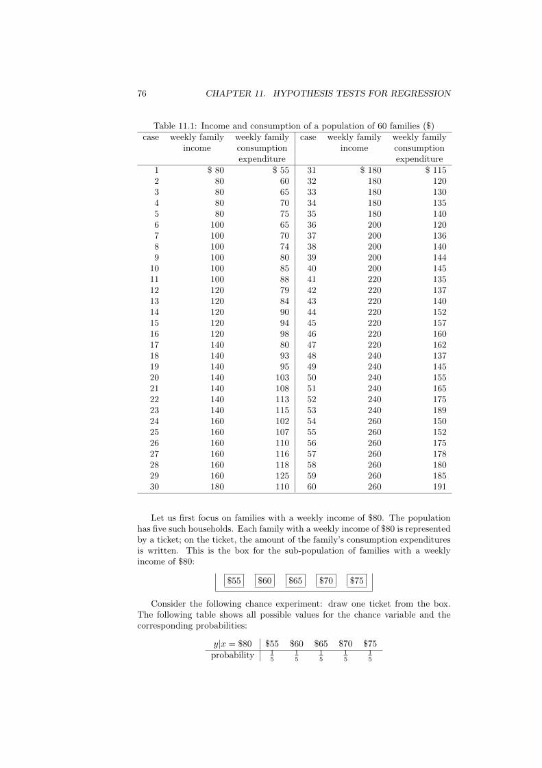
76 CHAPTER 11. HYPOTHESIS TESTS FOR REGRESSION
Table 11.1: Income and consumption of a population of 60 families ($)case weekly family weekly family case weekly family weekly family
income consumption income consumptionexpenditure expenditure
1 $ 80 $ 55 31 $ 180 $ 1152 80 60 32 180 1203 80 65 33 180 1304 80 70 34 180 1355 80 75 35 180 1406 100 65 36 200 1207 100 70 37 200 1368 100 74 38 200 1409 100 80 39 200 144
10 100 85 40 200 14511 100 88 41 220 13512 120 79 42 220 13713 120 84 43 220 14014 120 90 44 220 15215 120 94 45 220 15716 120 98 46 220 16017 140 80 47 220 16218 140 93 48 240 13719 140 95 49 240 14520 140 103 50 240 15521 140 108 51 240 16522 140 113 52 240 17523 140 115 53 240 18924 160 102 54 260 15025 160 107 55 260 15226 160 110 56 260 17527 160 116 57 260 17828 160 118 58 260 18029 160 125 59 260 18530 180 110 60 260 191
Let us first focus on families with a weekly income of $80. The populationhas five such households. Each family with a weekly income of $80 is representedby a ticket; on the ticket, the amount of the family’s consumption expendituresis written. This is the box for the sub-population of families with a weeklyincome of $80:
$55 $60 $65 $70 $75
Consider the following chance experiment: draw one ticket from the box.The following table shows all possible values for the chance variable and thecorresponding probabilities:
y|x = $80 $55 $60 $65 $70 $75probability 1
515
15
15
15
11.2. THE ERROR TERM 77
This table is the probability distribution of the consumption expenditures (y)for families with a weekly income of $80.
What are the expected consumption expenditures of households with a weeklyincome of $80? The expectation of a chance variable is the weighted average ofall possible values; the weights are the probabilities. This gives:
E(y|x = $80) = $55× 1
5+ $60× 1
5+ $65× 1
5+ $70× 1
5+ $75× 1
5= $65
Similarly, it can be shown that
E(y|x = $100) = $77E(y|x = $120) = $89E(y|x = $140) = $101E(y|x = $160) = $113E(y|x = $180) = $125E(y|x = $200) = $137E(y|x = $220) = $149E(y|x = $240) = $161E(y|x = $260) = $173
(Exercise 1 asks you to verify this for E(y|x = $180))The expected values are shown as black dots in figure 11.1. Verify with the
TI-84 that the points (x,E(y|x)) are on the straight line with equation:
E(y|x) = 0.6x+ 17
This equation is called the population regression function. It is shown asa solid line in the scatter plot (figure 11.1). The relationship between E(y|x)and x need not be a linear one, that is, a function that yields a straight linewhen you plot it, but we limit out attention to those cases where the populationregression function is a linear function:
E(y|x) = mx+ b
(or—in the case of multiple regression—a linear equation of the form E(y|x) =m1x1 +m2x2 + b).
11.2 The error term
Within each income class (a vertical strip in the scatter plot), we define theerror as the difference between the actual value of y and the expected value ofy:
error = actual− expected
For the five households with a weekly income of $80 the errors are:
error #1 = $55− $65 = −$10
error #2 = $60− $65 = −$5
error #3 = $65− $65 = $0
error #4 = $70− $65 = $5
error #5 = $75− $65 = $10
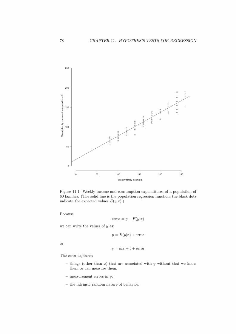
78 CHAPTER 11. HYPOTHESIS TESTS FOR REGRESSION
0 50 100 150 200 250
0
50
100
150
200
250
Weekly family income ($)
Wee
kly
fam
ily c
onsu
mpt
ion
expe
nditu
re ($
)
Figure 11.1: Weekly income and consumption expenditures of a population of60 families. (The solid line is the population regression function; the black dotsindicate the expected values E(y|x).)
Becauseerror = y − E(y|x)
we can write the values of y as:
y = E(y|x) + error
ory = mx+ b+ error
The error captures:
– things (other than x) that are associated with y without that we knowthem or can measure them;
– measurement errors in y;
– the intrinsic random nature of behavior.
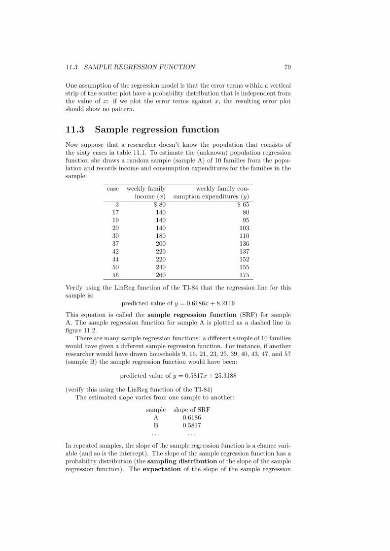
11.3. SAMPLE REGRESSION FUNCTION 79
One assumption of the regression model is that the error terms within a verticalstrip of the scatter plot have a probability distribution that is independent fromthe value of x: if we plot the error terms against x, the resulting error plotshould show no pattern.
11.3 Sample regression function
Now suppose that a researcher doesn’t know the population that consists ofthe sixty cases in table 11.1. To estimate the (unknown) population regressionfunction she draws a random sample (sample A) of 10 families from the popu-lation and records income and consumption expenditures for the families in thesample:
case weekly family weekly family con-income (x) sumption expenditures (y)
3 $ 80 $ 6517 140 8019 140 9520 140 10330 180 11037 200 13642 220 13744 220 15250 240 15556 260 175
Verify using the LinReg function of the TI-84 that the regression line for thissample is:
predicted value of y = 0.6186x+ 8.2116
This equation is called the sample regression function (SRF) for sampleA. The sample regression function for sample A is plotted as a dashed line infigure 11.2.
There are many sample regression functions: a different sample of 10 familieswould have given a different sample regression function. For instance, if anotherresearcher would have drawn households 9, 16, 21, 23, 25, 39, 40, 43, 47, and 57(sample B) the sample regression function would have been:
predicted value of y = 0.5817x+ 25.3188
(verify this using the LinReg function of the TI-84)The estimated slope varies from one sample to another:
sample slope of SRFA 0.6186B 0.5817
. . . . . .
In repeated samples, the slope of the sample regression function is a chance vari-able (and so is the intercept). The slope of the sample regression function has aprobability distribution (the sampling distribution of the slope of the sampleregression function). The expectation of the slope of the sample regression
80 CHAPTER 11. HYPOTHESIS TESTS FOR REGRESSION
0 50 100 150 200 250
0
50
100
150
200
250
Weekly family income ($)
Wee
kly
fam
ily c
onsu
mpt
ion
expe
nditu
re ($
)
Figure 11.2: Weekly income and consumption expenditures of a population of 60families. Note. The solid line is the population regression function, the dashedline is the sample regression function for sample A.
function is the typical value around which the slope of the sample regressionfunction varies in repeated samples (take a look at the sample estimates for theslope: do you have a hunch what the expectation is?).
It can be shown that the expectation of the slope of the sample regressionfunction (SRF) is the slope of the population regression function (PRF):
E(slope of the SRF) = slope of the PRF
That is, the slope of the sample regression function is an unbiased estimatorof the slope of the population regression function. This is only the case if theindependent variable (x) is not a chance variable (proof omitted).
The chance error for the slope is defined as:
chance error = slope of SRF− E(slope of SRF)
Now we can compute the chance errors that were made by each of the tworesearchers (of course, the researchers themselves can’t compute the chance
11.3. SAMPLE REGRESSION FUNCTION 81
error they made because they don’t know the population regression function).For sample A, the chance error of the slope is:
0.6186− 0.6000 = 0.0186
For sample B, the chance error of the slope is:
0.5817− 0.6000 = −0.0183
Here are the chance errors for samples A and B, and some other random samples:
sample slope of SRF chance error (without − sign)A 0.6186 0.0186 (0.0186)B 0.5817 −0.0183 (0.0183)C 0.6287 0.0287 (0.0287)D 0.6246 0.0246 (0.0246)E 0.5037 −0.0963 (0.0963)
. . . . . . . . . . . .typical value: expectation standard error
The standard error (SE) of the the slope of the sample regression functionis the typical size of the chance error (after you omitted the minus signs, asshown in the last column). The formula of the SE for the slope of the sampleregression function and uses information about the population. Unlike in thenumerical example above, in practice we don’t know the population. So howcan we find the SE of the slope of the sample regression function? The answeris that—just like when we estimated the SE for a sample average—we will usethe bootstrap and the sample data to find an estimate for the SE of the slope ofthe sample regression function. The formula is complicated and I won’t reportit here, but statistical software will compute an estimate of the SE based on thesample data. As in the case of the SE for an average, the SE for the slope of thesample regression function gets smaller if the sample size gets bigger: a biggerrandom sample tends to give a more precise estimate for the slope coefficient.
The same arguments apply to the intercept and—in multiple regression—theslope coefficients of the other independent variables.
Samples and populations
Suppose you have a data set covering all 50 states of the U.S. Some would arguethat such a data set covers a population (all the states of the U.S.), not a sample.Clearly the states were not randomly selected. Think however of the y values(on for each state) as generated by the following random process:
y = m1x+ b+ error = E(y|x) + error
The first part (m1x+b) is deterministic (determined by the population regressionfunction). The second part (the error term) is random: in terms of a box model,the error term is obtained by randomly drawing a ticket from a box with tickets;each ticket contains a value for the error term. Consider the data to be theresult of a natural experiment. As events unfold, “Nature” runs the experimentby drawing an error term from the box whenever a x takes a certain value. So aset of observations of x and the corresponding y can be considered as a randomsample, even when the observations cover all the possible subjects (such as all50 stated of the US): the chance is in the error terms, not in the cases.
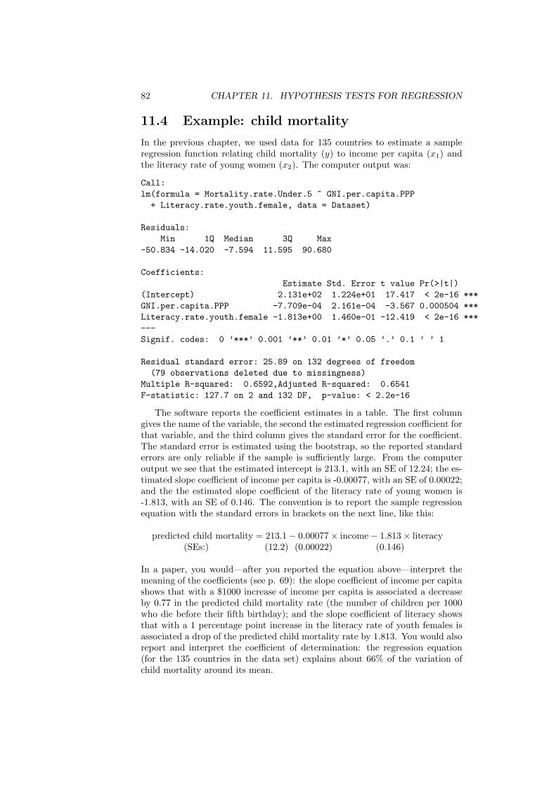
82 CHAPTER 11. HYPOTHESIS TESTS FOR REGRESSION
11.4 Example: child mortality
In the previous chapter, we used data for 135 countries to estimate a sampleregression function relating child mortality (y) to income per capita (x1) andthe literacy rate of young women (x2). The computer output was:
Call:
lm(formula = Mortality.rate.Under.5 ~ GNI.per.capita.PPP
+ Literacy.rate.youth.female, data = Dataset)
Residuals:
Min 1Q Median 3Q Max
-50.834 -14.020 -7.594 11.595 90.680
Coefficients:
Estimate Std. Error t value Pr(>|t|)
(Intercept) 2.131e+02 1.224e+01 17.417 < 2e-16 ***
GNI.per.capita.PPP -7.709e-04 2.161e-04 -3.567 0.000504 ***
Literacy.rate.youth.female -1.813e+00 1.460e-01 -12.419 < 2e-16 ***
---
Signif. codes: 0 ’***’ 0.001 ’**’ 0.01 ’*’ 0.05 ’.’ 0.1 ’ ’ 1
Residual standard error: 25.89 on 132 degrees of freedom
(79 observations deleted due to missingness)
Multiple R-squared: 0.6592,Adjusted R-squared: 0.6541
F-statistic: 127.7 on 2 and 132 DF, p-value: < 2.2e-16
The software reports the coefficient estimates in a table. The first columngives the name of the variable, the second the estimated regression coefficient forthat variable, and the third column gives the standard error for the coefficient.The standard error is estimated using the bootstrap, so the reported standarderrors are only reliable if the sample is sufficiently large. From the computeroutput we see that the estimated intercept is 213.1, with an SE of 12.24; the es-timated slope coefficient of income per capita is -0.00077, with an SE of 0.00022;and the the estimated slope coefficient of the literacy rate of young women is-1.813, with an SE of 0.146. The convention is to report the sample regressionequation with the standard errors in brackets on the next line, like this:
predicted child mortality = 213.1− 0.00077× income− 1.813× literacy(SEs:) (12.2) (0.00022) (0.146)
In a paper, you would—after you reported the equation above—interpret themeaning of the coefficients (see p. 69): the slope coefficient of income per capitashows that with a $1000 increase of income per capita is associated a decreaseby 0.77 in the predicted child mortality rate (the number of children per 1000who die before their fifth birthday); and the slope coefficient of literacy showsthat with a 1 percentage point increase in the literacy rate of youth females isassociated a drop of the predicted child mortality rate by 1.813. You would alsoreport and interpret the coefficient of determination: the regression equation(for the 135 countries in the data set) explains about 66% of the variation ofchild mortality around its mean.
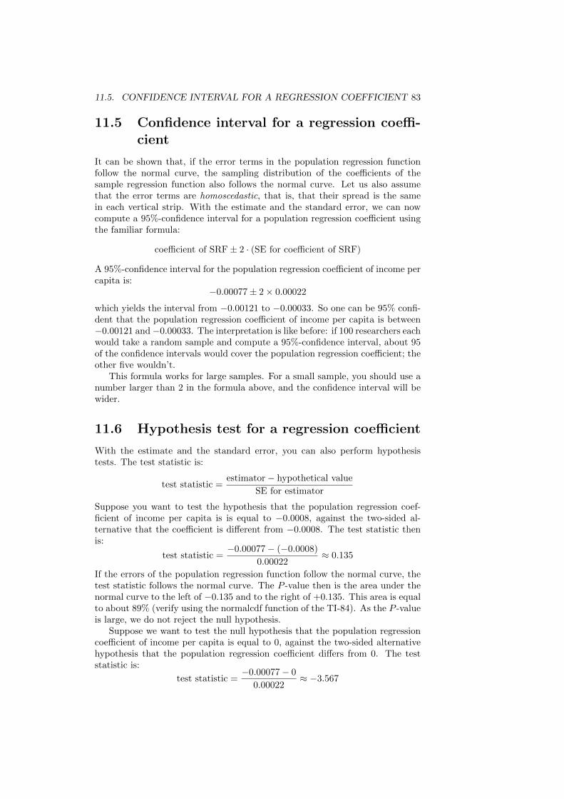
11.5. CONFIDENCE INTERVAL FOR A REGRESSION COEFFICIENT 83
11.5 Confidence interval for a regression coeffi-cient
It can be shown that, if the error terms in the population regression functionfollow the normal curve, the sampling distribution of the coefficients of thesample regression function also follows the normal curve. Let us also assumethat the error terms are homoscedastic, that is, that their spread is the samein each vertical strip. With the estimate and the standard error, we can nowcompute a 95%-confidence interval for a population regression coefficient usingthe familiar formula:
coefficient of SRF± 2 · (SE for coefficient of SRF)
A 95%-confidence interval for the population regression coefficient of income percapita is:
−0.00077± 2× 0.00022
which yields the interval from −0.00121 to −0.00033. So one can be 95% confi-dent that the population regression coefficient of income per capita is between−0.00121 and−0.00033. The interpretation is like before: if 100 researchers eachwould take a random sample and compute a 95%-confidence interval, about 95of the confidence intervals would cover the population regression coefficient; theother five wouldn’t.
This formula works for large samples. For a small sample, you should use anumber larger than 2 in the formula above, and the confidence interval will bewider.
11.6 Hypothesis test for a regression coefficient
With the estimate and the standard error, you can also perform hypothesistests. The test statistic is:
test statistic =estimator− hypothetical value
SE for estimator
Suppose you want to test the hypothesis that the population regression coef-ficient of income per capita is is equal to −0.0008, against the two-sided al-ternative that the coefficient is different from −0.0008. The test statistic thenis:
test statistic =−0.00077− (−0.0008)
0.00022≈ 0.135
If the errors of the population regression function follow the normal curve, thetest statistic follows the normal curve. The P -value then is the area under thenormal curve to the left of −0.135 and to the right of +0.135. This area is equalto about 89% (verify using the normalcdf function of the TI-84). As the P -valueis large, we do not reject the null hypothesis.
Suppose we want to test the null hypothesis that the population regressioncoefficient of income per capita is equal to 0, against the two-sided alternativehypothesis that the population regression coefficient differs from 0. The teststatistic is:
test statistic =−0.00077− 0
0.00022≈ −3.567
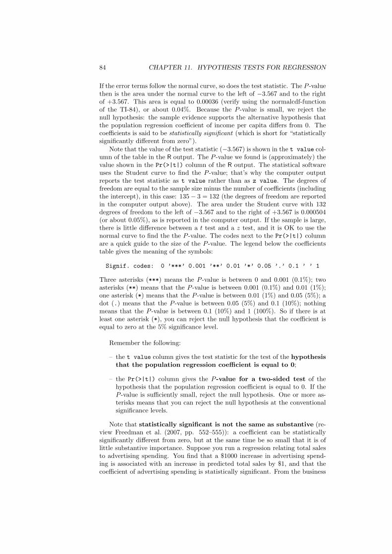
84 CHAPTER 11. HYPOTHESIS TESTS FOR REGRESSION
If the error terms follow the normal curve, so does the test statistic. The P -valuethen is the area under the normal curve to the left of −3.567 and to the rightof +3.567. This area is equal to 0.00036 (verify using the normalcdf-functionof the TI-84), or about 0.04%. Because the P -value is small, we reject thenull hypothesis: the sample evidence supports the alternative hypothesis thatthe population regression coefficient of income per capita differs from 0. Thecoefficients is said to be statistically significant (which is short for “statisticallysignificantly different from zero”).
Note that the value of the test statistic (−3.567) is shown in the t value col-umn of the table in the R output. The P -value we found is (approximately) thevalue shown in the Pr(>|t|) column of the R output. The statistical softwareuses the Student curve to find the P -value; that’s why the computer outputreports the test statistic as t value rather than as z value. The degrees offreedom are equal to the sample size minus the number of coefficients (includingthe intercept), in this case: 135− 3 = 132 (the degrees of freedom are reportedin the computer output above). The area under the Student curve with 132degrees of freedom to the left of −3.567 and to the right of +3.567 is 0.000504(or about 0.05%), as is reported in the computer output. If the sample is large,there is little difference between a t test and a z test, and it is OK to use thenormal curve to find the the P -value. The codes next to the Pr(>|t|) columnare a quick guide to the size of the P -value. The legend below the coefficientstable gives the meaning of the symbols:
Signif. codes: 0 ’***’ 0.001 ’**’ 0.01 ’*’ 0.05 ’.’ 0.1 ’ ’ 1
Three asterisks (***) means the P -value is between 0 and 0.001 (0.1%); twoasterisks (**) means that the P -value is between 0.001 (0.1%) and 0.01 (1%);one asterisk (*) means that the P -value is between 0.01 (1%) and 0.05 (5%); adot (.) means that the P -value is between 0.05 (5%) and 0.1 (10%); nothingmeans that the P -value is between 0.1 (10%) and 1 (100%). So if there is atleast one asterisk (*), you can reject the null hypothesis that the coefficient isequal to zero at the 5% significance level.
Remember the following:
– the t value column gives the test statistic for the test of the hypothesisthat the population regression coefficient is equal to 0;
– the Pr(>|t|) column gives the P -value for a two-sided test of thehypothesis that the population regression coefficient is equal to 0. If theP -value is sufficiently small, reject the null hypothesis. One or more as-terisks means that you can reject the null hypothesis at the conventionalsignificance levels.
Note that statistically significant is not the same as substantive (re-view Freedman et al. (2007, pp. 552–555)): a coefficient can be statisticallysignificantly different from zero, but at the same time be so small that it is oflittle substantive importance. Suppose you run a regression relating total salesto advertising spending. You find that a $1000 increase in advertising spend-ing is associated with an increase in predicted total sales by $1, and that thecoefficient of advertising spending is statistically significant. From the business
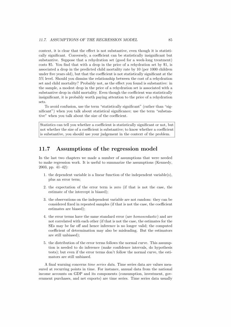
11.7. ASSUMPTIONS OF THE REGRESSION MODEL 85
context, it is clear that the effect is not substantive, even though it is statisti-cally significant. Conversely, a coefficient can be statistically insignificant butsubstantive. Suppose that a rehydration set (good for a week-long treatment)costs $5. You find that with a drop in the price of a rehydration set by $1, isassociated a drop in the predicted child mortality rate by 10 (per 1000 childrenunder five years old), but that the coefficient is not statistically significant at the5% level. Should you dismiss the relationship between the cost of a rehydrationset and child mortality? Probably not, as the effect you found is substantive: inthe sample, a modest drop in the price of a rehydration set is associated with asubstantive drop in child mortality. Even though the coefficient was statisticallyinsignificant, it is probably worth paying attention to the price of a rehydrationsets.
To avoid confusion, use the term “statistically significant” (rather than “sig-nificant”) when you talk about statistical significance; use the term “substan-tive” when you talk about the size of the coefficient.
Statistics can tell you whether a coefficient is statistically significant or not, butnot whether the size of a coefficient is substantive; to know whether a coefficientis substantive, you should use your judgement in the context of the problem.
11.7 Assumptions of the regression model
In the last two chapters we made a number of assumptions that were neededto make regression work. It is useful to summarize the assumptions (Kennedy,2003, pp. 41–42):
1. the dependent variable is a linear function of the independent variable(s),plus an error term;
2. the expectation of the error term is zero (if that is not the case, theestimate of the intercept is biased);
3. the observations on the independent variable are not random: they can beconsidered fixed in repeated samples (if that is not the case, the coefficientestimates are biased);
4. the error terms have the same standard error (are homoscedastic) and arenot correlated with each other (if that is not the case, the estimates for theSEs may be far off and hence inference is no longer valid; the computedcoefficient of determination may also be misleading. But the estimatorsare still unbiased);
5. the distribution of the error terms follows the normal curve. This assump-tion is needed to do inference (make confidence intervals, do hypothesistests); but even if the error terms don’t follow the normal curve, the esti-mators are still unbiased.
A final warning concerns time series data. Time series data are values mea-sured at recurring points in time. For instance, annual data from the nationalincome accounts on GDP and its components (consumption, investment, gov-ernment purchases, and net exports) are time series. Time series data usually
86 CHAPTER 11. HYPOTHESIS TESTS FOR REGRESSION
are notated with a time index (yt, xt). A time series of n observations of thevariable yt is a list that looks like this:
{y1, y2, y3, . . . , yt, . . . yn}
where y1 is the value of y (say, consumption) observed in the first period (say,the year 2000), y2 is the value of y observed in the second period (the year2001), and so on.
It turns out that many time series have a statistical property called non-stationarity. Amongst other things, the presence of a time trend in thedata (a tendency for the values to go up or down over time) will make a seriesnon-stationary. To spot a possible time trend, it is a good idea to plot a timeseries diagram of each time series. A time series diagram is a line diagramwith time (t) on the horizontal axis and the time series (yt on the vertical axis(include figure as example). If the data are non-stationary, the resultsof regression (and of inference based on regression) may be wrong.Be cautious if your data are time series. Two easy fixes may work: include thetime variable t as one of the independent variables in the multiple regression, oruse the change in y and the change in x in the regression. Still, if you suspectnon-stationarity, consult someone who knows how to deal with it.
11.8 Questions for Review
1. What is a population regression function?
2. How is the error of regression defined? What does it capture?
3. What is a sample regression function?
4. Why does an estimated sample regression function differ from the popu-lation regression function?
5. What does it mean that the slope of the sample regression function is anunbiased estimator of the slope of the population regression function?
6. How is the chance error of the slope defined?
7. What does the standard error (SE) of the the slope of the sample regressionfunction measure?
8. Given that in practice we don’t know the population, how can we estimatethe standard error (SE) of the the slope of the sample regression function?
9. What happens to the standard error (SE) of the slope of the sample re-gression function if (other things equal) the sample gets bigger?
10. How do you compute a 95% confidence interval for the slope of the pop-ulation regression function? Under which conditions can you apply theformula?
11. How do you interpret a 95% confidence interval for the slope of the popula-tion regression function? Give the exact probability interpretation, usingthe concept of repeated samples.
11.9. EXERCISES 87
12. How do you compute the test statistic for a test on a coefficient from aregression?
13. Suppose that you want to test the null hypothesis that a coefficient of thepopulation regression is equal to zero. How do you interpret the P -valuefor the test?
14. What does the column Estimate in computer regression output report?
15. What does the column Std. Error in computer regression output re-port?
16. What does the column t value in computer regression output report?
17. What does the column Pr(>|t|) in computer regression output report?
18. What is the meaning of the Residual standard error in computer re-gression output?
19. What is the meaning of the R-squared in computer regression output?
20. What are the assumptions underlying the multiple regression model usedin this chapter?
21. What are time series data? Illustrate using an example.
22. Why should you be careful when the multiple regression model for timeseries data?
11.9 Exercises
1. For the example in section 11.1, verify that E(y|x = $180) = $125. Showyour work.
2. Find a 95%-confidence interval for the population regression coefficient ofthe literacy rate in the child mortality regression. Give the probability inter-pretation of a 95%-confidence interval. Which assumptions did you have tomake?
3. For 14 systems analysts, their annual salaries (in $), years of experience,and years of postsecondary education were recorded (Kazmier, 1995, table 15.2p. 275) (same regression as in the exercise of the previous chapter). Below isthe computer output for the multiple regression of the annual salaries on theyears of experience and the years of postsecondary education:
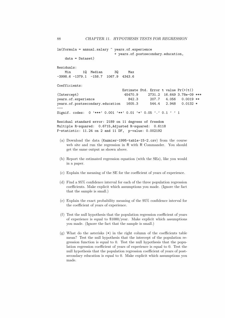
88 CHAPTER 11. HYPOTHESIS TESTS FOR REGRESSION
lm(formula = annual.salary ~ years.of.experience
+ years.of.postsecondary.education,
data = Dataset)
Residuals:
Min 1Q Median 3Q Max
-3998.6 -1379.1 -158.7 1067.9 4343.6
Coefficients:
Estimate Std. Error t value Pr(>|t|)
(Intercept) 45470.9 2731.2 16.649 3.78e-09 ***
years.of.experience 842.3 207.7 4.056 0.0019 **
years.of.postsecondary.education 1605.3 544.4 2.948 0.0132 *
---
Signif. codes: 0 ’***’ 0.001 ’**’ 0.01 ’*’ 0.05 ’.’ 0.1 ’ ’ 1
Residual standard error: 2189 on 11 degrees of freedom
Multiple R-squared: 0.6715,Adjusted R-squared: 0.6118
F-statistic: 11.24 on 2 and 11 DF, p-value: 0.002192
(a) Download the data (Kazmier-1995-table-15-2.csv) from the courseweb site and run the regression in R with R Commander. You shouldget the same output as shown above.
(b) Report the estimated regression equation (with the SEs), like you wouldin a paper.
(c) Explain the meaning of the SE for the coefficient of years of experience.
(d) Find a 95% confidence interval for each of the three population regressioncoefficients. Make explicit which assumptions you made. (Ignore the factthat the sample is small.)
(e) Explain the exact probability meaning of the 95% confidence interval forthe coefficient of years of experience.
(f) Test the null hypothesis that the population regression coefficient of yearsof experience is equal to $1000/year. Make explicit which assumptionsyou made. (Ignore the fact that the sample is small.)
(g) What do the asterisks (*) in the right column of the coefficients tablemean? Test the null hypothesis that the intercept of the population re-gression function is equal to 0. Test the null hypothesis that the popu-lation regression coefficient of years of experience is equal to 0. Test thenull hypothesis that the population regression coefficient of years of post-secondary education is equal to 0. Make explicit which assumptions youmade.
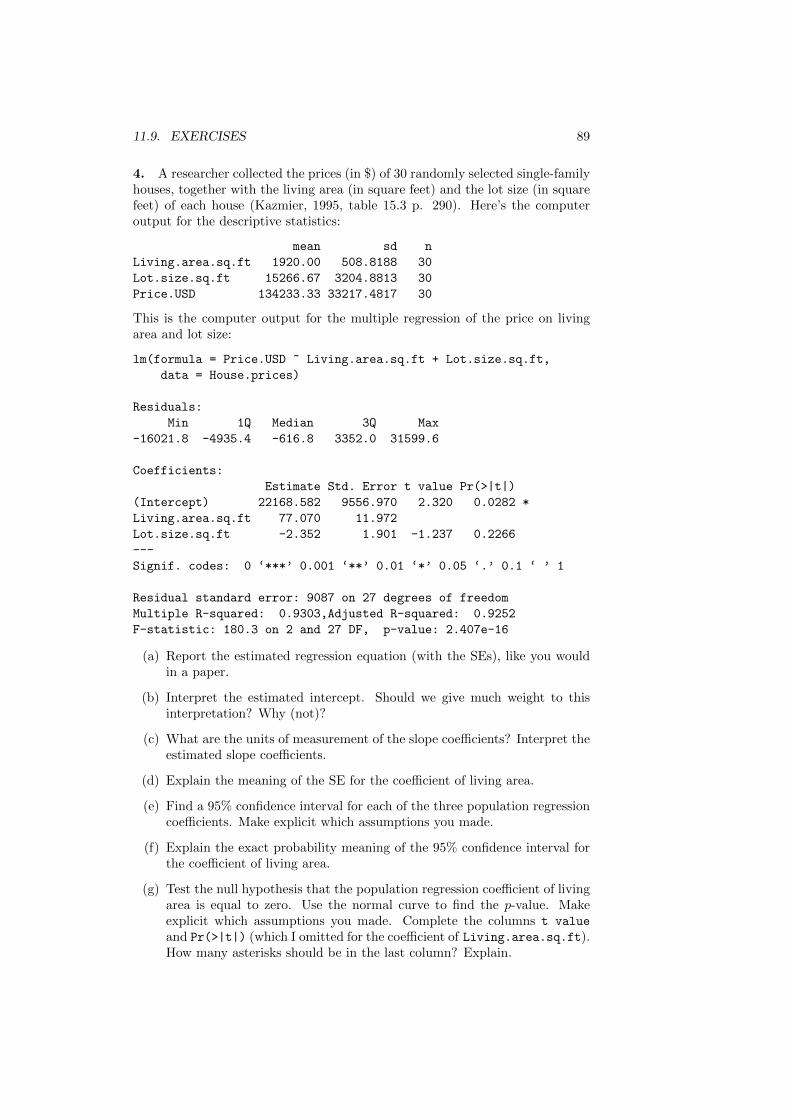
11.9. EXERCISES 89
4. A researcher collected the prices (in $) of 30 randomly selected single-familyhouses, together with the living area (in square feet) and the lot size (in squarefeet) of each house (Kazmier, 1995, table 15.3 p. 290). Here’s the computeroutput for the descriptive statistics:
mean sd n
Living.area.sq.ft 1920.00 508.8188 30
Lot.size.sq.ft 15266.67 3204.8813 30
Price.USD 134233.33 33217.4817 30
This is the computer output for the multiple regression of the price on livingarea and lot size:
lm(formula = Price.USD ~ Living.area.sq.ft + Lot.size.sq.ft,
data = House.prices)
Residuals:
Min 1Q Median 3Q Max
-16021.8 -4935.4 -616.8 3352.0 31599.6
Coefficients:
Estimate Std. Error t value Pr(>|t|)
(Intercept) 22168.582 9556.970 2.320 0.0282 *
Living.area.sq.ft 77.070 11.972
Lot.size.sq.ft -2.352 1.901 -1.237 0.2266
---
Signif. codes: 0 ‘***’ 0.001 ‘**’ 0.01 ‘*’ 0.05 ‘.’ 0.1 ‘ ’ 1
Residual standard error: 9087 on 27 degrees of freedom
Multiple R-squared: 0.9303,Adjusted R-squared: 0.9252
F-statistic: 180.3 on 2 and 27 DF, p-value: 2.407e-16
(a) Report the estimated regression equation (with the SEs), like you wouldin a paper.
(b) Interpret the estimated intercept. Should we give much weight to thisinterpretation? Why (not)?
(c) What are the units of measurement of the slope coefficients? Interpret theestimated slope coefficients.
(d) Explain the meaning of the SE for the coefficient of living area.
(e) Find a 95% confidence interval for each of the three population regressioncoefficients. Make explicit which assumptions you made.
(f) Explain the exact probability meaning of the 95% confidence interval forthe coefficient of living area.
(g) Test the null hypothesis that the population regression coefficient of livingarea is equal to zero. Use the normal curve to find the p-value. Makeexplicit which assumptions you made. Complete the columns t value
and Pr(>|t|) (which I omitted for the coefficient of Living.area.sq.ft).How many asterisks should be in the last column? Explain.

90 CHAPTER 11. HYPOTHESIS TESTS FOR REGRESSION
(h) Interpret the r.m.s. error of regression (Residual standard error in thecomputer output).
(i) Interpret the R2 (R-squared in the computer output).
(j) Download the data (Kazmier-1995-table-15-3.csv) from the courseweb site and run the regression with R Commander. You should get thesame output as shown above.

Chapter 12
The Chi-Square test
Read Freedman et al. (2007, Ch. 28). Skip the explanation of how to use χ2-tables (starting on p. 527 with “In principle, there is one table . . . ” and endingwith the sketch on the top of p. 528); statisticians use a statistical calculator orstatistical software to find areas under the χ2-curve. Also skip section 3 (“HowFisher used the χ2-test”), pp. 533–535.
Questions for Review
1. When should the χ2-test be used, as opposed to the z-test?
2. What are the six ingredients of a χ2-test?
12.1 Exercises
Work the following exercises from Freedman et al. (2007), chapter 28: Set A: 1,2, 3, 4, 7, 8. Set C: 2. Review exercises: 7.
91

92 CHAPTER 12. THE CHI-SQUARE TEST

Bibliography
Freedman, D., Pisani, R., and Purves, R. (2007). Statistics. Norton, New Yorkand London, 4th edition.
Garcia, J. and Quintana-Domeque, C. (2007). The evolution of adult height inEurope: A brief note. Economics & Human Biology, 5(2):340–349.
Gujarati, D. N. (2003). Basic Econometrics. McGraw-Hill, Boston, 4th edition.
Heston, A., Summers, R., and Aten, B. (2012). Penn World Table Version 7.1.Center for International Comparisons of Production, Income and Prices atthe University of Pennsylvania, Philadelphia.
Kazmier, L. J. (1995). Schaum’s Outline of Theory and Problems of BusinessStatistics. Schaum’s Outline Series. McGraw-Hill, New York.
Kennedy, P. (2003). A Guide to Econometrics. Blackwell, Malden, MA, 6th
edition.
Moore, D. S., McCabe, G. P., and Craig, B. A. (2012). Introduction to thePractice of Statistics. Freeman, New York, 7th edition.
Rosling, H. (2015). No more rich world and poor world – Don’t panic: How toend poverty in 15 years – BBC Two. (video).
World Bank (2013). World Bank Open Data. Consulted on 21 November 2013on http://data.worldbank.org.
93